NAVAL POSTGRADUATE SCHOOL - Defense … · iii Approved for public release; distribution is...

NAVAL POSTGRADUATE

SCHOOL

MONTEREY, CALIFORNIA

MBA PROFESSIONAL REPORT

THE EFFECT OF ZONING LAWS ON HOUSING PRICES AND BAH RATES

December 2014

By: William Fitzkee Advisors: David Henderson Amilcar Menichini

Approved for public release; distribution is unlimited

THIS PAGE INTENTIONALLY LEFT BLANK

i

REPORT DOCUMENTATION PAGE Form Approved OMB No. 0704-0188 Public reporting burden for this collection of information is estimated to average 1 hour per response, including the time for reviewing instruction, searching existing data sources, gathering and maintaining the data needed, and completing and reviewing the collection of information. Send comments regarding this burden estimate or any other aspect of this collection of information, including suggestions for reducing this burden, to Washington headquarters Services, Directorate for Information Operations and Reports, 1215 Jefferson Davis Highway, Suite 1204, Arlington, VA 22202-4302, and to the Office of Management and Budget, Paperwork Reduction Project (0704-0188) Washington DC 20503. 1. AGENCY USE ONLY (Leave blank)

2. REPORT DATE December 2014

3. REPORT TYPE AND DATES COVERED MBA Professional Report

4. TITLE AND SUBTITLE THE EFFECT OF ZONING LAWS ON HOUSING PRICES AND BAH RATES

5. FUNDING NUMBERS

6. AUTHOR(S) William Fitzkee 7. PERFORMING ORGANIZATION NAME(S) AND ADDRESS(ES)

Naval Postgraduate School Monterey, CA 93943-5000

8. PERFORMING ORGANIZATION REPORT NUMBER

9. SPONSORING /MONITORING AGENCY NAME(S) AND ADDRESS(ES) N/A

10. SPONSORING/MONITORING AGENCY REPORT NUMBER

11. SUPPLEMENTARY NOTES The views expressed in this thesis are those of the author and do not reflect the official policy or position of the Department of Defense or the U.S. Government. IRB Protocol number ____N/A____.

12a. DISTRIBUTION / AVAILABILITY STATEMENT Approved for public release; distribution is unlimited

12b. DISTRIBUTION CODE

13. ABSTRACT (maximum 200 words)

This thesis is an analysis of the effect of zoning laws and regulations on the price of residential housing. Economists Edward Glaeser and Joseph Gyourko have completed significant work on this topic. Their efforts have focused on the correlation of high housing prices with zoning laws and other land-use controls, but stop short of estimating the impact of zoning laws on actual housing prices in specific markets. This thesis expands on their research and estimates what residential housing prices would be without the regulations. It also estimates the deadweight loss (DWL) caused by the zoning laws in various high-cost markets. The results show significant price reductions from both complete and partial elimination of zoning restrictions. This thesis also uses these estimates to calculate the impact of the zoning laws on Basic Allowance for Housing (BAH) in the markets analyzed. Estimated BAH rates with zoning reduced or eliminated were substantially lower in many of the high-cost housing markets studied.

14. SUBJECT TERMS zoning laws, land-use restrictions, housing prices, basic allowance for housing, housing supply

15. NUMBER OF PAGES

63 16. PRICE CODE

17. SECURITY CLASSIFICATION OF REPORT

Unclassified

18. SECURITY CLASSIFICATION OF THIS PAGE

Unclassified

19. SECURITY CLASSIFICATION OF ABSTRACT

Unclassified

20. LIMITATION OF ABSTRACT

UU NSN 7540-01-280-5500 Standard Form 298 (Rev. 2-89) Prescribed by ANSI Std. 239-18

ii


iii

Approved for public release; distribution is unlimited


William Fitzkee, Lieutenant Commander, United States Navy

Submitted in partial fulfillment of the requirements for the degree of

MASTER OF BUSINESS ADMINISTRATION

from the

NAVAL POSTGRADUATE SCHOOL December 2014

Author: William Fitzkee Approved by: David Henderson Amilcar Menichini William R. Gates, Dean

Graduate School of Business and Public Policy

iv


v


ABSTRACT

This thesis is an analysis of the effect of zoning laws and regulations on the price of

residential housing. Economists Edward Glaeser and Joseph Gyourko have completed

significant work on this topic. Their efforts have focused on the correlation of high

housing prices with zoning laws and other land-use controls, but stop short of estimating

the impact of zoning laws on actual housing prices in specific markets. This thesis

expands on their research and estimates what residential housing prices would be without

the regulations. It also estimates the deadweight loss (DWL) caused by the zoning laws in

various high-cost markets. The results show significant price reductions from both

complete and partial elimination of zoning restrictions. This thesis also uses these

estimates to calculate the impact of the zoning laws on Basic Allowance for Housing

(BAH) in the markets analyzed. Estimated BAH rates with zoning reduced or eliminated

were substantially lower in many of the high-cost housing markets studied.

vi


vii

TABLE OF CONTENTS

I. INTRODUCTION .......................................................................................................1

II. LITERATURE REVIEW ...........................................................................................5 A. ZONING LAWS AND LAND-USE REGULATIONS .................................5 B. ECONOMIC IMPACT OF ZONING LAWS ON HOUSE PRICES .........8 C. ZONING LAWS VERSUS LAND AVAILABILITY .................................15

III. ANALYSIS .................................................................................................................19 A. CALCULATION OF P WITHOUT ZONING TAX ..................................19 B. CALCULATION OF Q WITHOUT ZONING TAX .................................25 C. CALCULATION OF DWL AND ZONING TAX ......................................31 D. REGRESSION ANALYSIS OF DWL AND REGULATION ...................32

IV. NET EFFECT ON BAH RATES .............................................................................35 A. BAH METHODOLOGY ...............................................................................35 B. CALCULATION OF BAH RATES WITHOUT ZONING TAX .............36

V. CONCLUSION ..........................................................................................................41 LIST OF REFERENCES ......................................................................................................43

INITIAL DISTRIBUTION LIST .........................................................................................47

viii


ix

LIST OF FIGURES

Figure 1. Shift in the Supply Curve from Zoning .............................................................9 Figure 2. Decrease in Elasticity of the Supply Curve from Zoning ................................10 Figure 3. Incidence and DWL of the Zoning Tax ...........................................................13

x


xi

LIST OF TABLES

Table 1. Intensive versus Imputed Cost of Land in 26 Metropolitan Areas (from Glaeser & Gyourko, 2002) ...............................................................................17

Table 2. Zoning Tax Ratio and CC / sq. ft. ....................................................................21 Table 3. Implicit Zoning Tax Percentage .......................................................................22 Table 4. Equilibrium Price without the Zoning Tax (P) ................................................24 Table 5. Equilibrium Quantity without Zoning Tax (Q) [ηd = -.3] ................................27 Table 6. Equilibrium Quantity without Zoning Tax (Q) [ηd = -.5] ................................28 Table 7. Equilibrium Quantity without Zoning Tax (Q) [ηd = -.7] ................................29 Table 8. Equilibrium Quantity without Zoning Tax (Q) [ηd = -.9] ................................30 Table 9. Estimated DWL ...............................................................................................31 Table 10. Regulation Index ..............................................................................................33 Table 11. Linear Regression of DWL on Regulation Index ............................................34 Table 12. BAH Rates .......................................................................................................38 Table 13. BAH Rates with Zoning Tax Reduction ..........................................................39 Table 14. Linear Regression of BAH Rate on PI .............................................................40

xii


xiii

LIST OF ACRONYMS AND ABBREVIATIONS

ACS American Community Survey

AHS American Housing Survey BAH Basic Allowance for Housing

CC construction costs DOA Department of the Army

DOAF Department of the Air Force DOD Department of Defense

DON Department of the Navy DTMO Defense Travel Management Office

DWL deadweight loss HOA homeowner association

MHA Military Housing Area NAHB National Association of Home Builders

OUSD(C) Office of the Under Secretary of Defense (Comptroller) P equilibrium price without zoning regulation

P75 equilibrium price with a 75% reduction in zoning regulation

P50 equilibrium price with a 50% reduction in zoning regulation

PI price prime, equilibrium price with zoning regulation

Q equilibrium quantity supplied without zoning regulation Q75 equilibrium quantity supplied with a 75% zoning reduction

Q50 equilibrium quantity supplied with a 50% zoning reduction

QI quantity prime, equilibrium quantity supplied with zoning

USA United States Army USAF United States Air Force

USMC United States Marine Corps ηd price elasticity of demand

ηs price elasticity of supply

xiv


1

I. INTRODUCTION

Zoning laws and other land-use restrictions can have a significant impact on the

price of housing. Housing costs can be decomposed into three elements; construction

costs (CC), the cost of land, and the costs associated with obtaining the legal right to

build a structure on the land (Glaeser, Gyourko, & Saks, 2005). Since 1970, construction

costs for housing have declined in real terms, yet during that same period real housing

prices in the United States have steadily climbed an average of 1.7% annually (Glaeser et

al., 2005). In some markets these increases have been much greater. The main driver of

this increase in housing costs appears to be government regulation in the form of zoning

laws and various other types of land-use restrictions and taxes (Glaeser & Gyourko,

2002). Many of these restrictions impose artificial limits on the supply of housing, and

the result is housing prices that are well above the actual cost of construction and the

implicit value of the land (Glaeser & Gyourko, 2002). Other types of land-use regulations

act like a tax on the construction of new housing. Both forms of zoning regulation result

in a higher market equilibrium price for housing, lower equilibrium quantity, and an

associated deadweight loss (DWL). The aggregate effect of all zoning regulations and

land-use restrictions in a metropolitan area is referred to as the zoning “tax.” The increase

in price and the size of the DWL will vary depending on the amount of zoning regulation

(size of the zoning tax), and the price elasticity of supply and demand.

Glaeser and Gyourko (2002) proved that the steep prices seen in various high-cost

housing markets was the result of zoning regulation as opposed to the traditional

economic view of land scarcity. This paper furthers their research and explores the effect

of zoning on housing prices, specifically calculating what the price would be without

zoning or with a reduction in zoning regulation. In addition, the DWL that is associated

with zoning regulations is calculated. A linear regression of the calculated DWL for each

metropolitan area on an index that measures the level of regulation is conducted to test

the correlation between DWL and the level of land-use restrictions. Lastly, the impact of

zoning regulations on Basic Allowance for Housing (BAH) rates, which is a sizeable

portion of the Department of Defense (DOD) budget, is analyzed. Specifically, the

2

potential price reductions for housing from the elimination or easing of zoning

regulations are applied to the BAH rate calculation methodology to determine what BAH

rates would be without zoning regulation or with reduced zoning in the markets studied.

Using the data from Glaeser and Gyourko (2002), a range of potential percentage

price decreases is calculated for each market studied. There is no way to directly measure

or calculate with complete certainty what housing prices would be without land-use

restrictions. The method chosen in this paper utilizes Glaeser and Gyourko’s (2002)

calculations for the implicit price of land from the hedonic method and the extensive

value of land including zoning taxes. Comparing these two values gives the percentage of

the median housing price that is above construction costs (CC) attributable to zoning

regulation. The result is an implicit zoning tax percentage for each market studied. This

implicit zoning tax percentage is then subtracted from the median housing price for

owner-occupied housing from the 2012 American Community Survey (ACS) to calculate

what the price would be without any zoning regulation, which is referred to as the

equilibrium price (P). P for a 75% zoning reduction and a 50% zoning reduction is also

calculated to give a realistic range for the amount of zoning regulation that could feasibly

be eliminated in an effort by local governments to make housing more affordable.

The median price of owner-occupied housing with zoning regulation is referred to

as equilibrium price prime (PI). The equilibrium quantity supplied with zoning is called

QI. These values are obtained from the 2012 ACS for the markets studied by Glaeser and

Gyourko (2002). This paper uses a range of values for the price elasticity of housing

demand (ηd) that have been estimated in previous studies by Muth (1971), Polinsky and

Ellwood (1979), and Hanushek and Quigley (1980). The ηd values used are -.3, -.5, -.7,

and -.9. With PI, QI, the calculated P values, and ηd, we can determine the quantity

supplied without zoning regulation and for various levels of zoning reduction. This value

is referred to as Q.

With Q and P values for a 100% zoning regulation reduction and ηd of -.5, the

DWL associated with the zoning tax in the various markets studied is calculated. This

DWL represents the loss to society that is a result of the zoning regulations. A linear

3

regression is then performed of these estimated DWL values on the regulatory index

values from Malpezzi (1996).

The final portion of the paper examines how land-use restrictions affect BAH

rates. The 2012 BAH rates for the markets studied are obtained from Defense Travel

Management Office (DTMO). BAH rates are calculated using estimated median market

rent prices for various types of dwellings depending on the rank of the service member

and dependent status. The types of dwellings used range from apartments to detached

single-family homes. The average cost of utilities and renter’s insurance is also factored

into the BAH rate calculation. DTMO provides a BAH component breakdown that

specifies an average percentage for the rent portion of the BAH rate in each market. This

is the portion of BAH that is affected by zoning regulation.

Rent and house prices are highly correlated. The rent-price ratio is the metric

typically used to describe this relationship. The rent-price ratio is calculated by dividing

average annual rent by median price. Historically, the rent-price has averaged 5%, with

little variation (Davis, Lehnert, & Martin, 2008). Any reduction in the price of housing is

going to correlate to a proportional reduction in market rent. Using the calculated implicit

zoning tax percentage, BAH rates for a 100%, 75%, and 50% reduction to the zoning tax

are estimated for each metropolitan area.

4


5

II. LITERATURE REVIEW

A. ZONING LAWS AND LAND-USE REGULATIONS

The subject of zoning is a complex and vast subject that overlaps multiple

academic areas, including economics, the law, and other social sciences. This paper

focuses on the economic aspect of the zoning and land-use restrictions prevalent in

municipalities across the United States. A brief history of zoning and its different forms

follows. This paper uses the terms zoning and land-use restrictions interchangeably to

describe any type of zoning law.

According to Deakin (1989) there are five general categories of zoning and land-

use restrictions:

1. Restrictions on location, density, and intensity of development

2. Regulations on design and performance for lots and structures

3. Costs levied on building developers for new construction

4. Moratorium on development in specific areas

5. Various controls on growth of buildings and population

These categories are broad and include many different types of laws that control

the use and development of land. The first category includes the traditional zoning for

residential or commercial use of land. Also in this category are the laws that mandate

minimum lot sizes and the type of residential structures (i.e. single-family detached,

multi-family, apartment, etc.). Most zoning laws in this country prior to 1970 fall into this

category (Fischel, 2004). The second category essentially covers the building codes. The

third category includes fees levied by local governments on developers and the overall

permit and approval process. This category can be considerably costly because of the

delays that are involved. Categories four and five are land-use regulations designed to

either prevent or control growth. Most of the zoning laws that fall under these last two

categories have been implemented from the early 1970s onward, and generally in

suburban areas of the United States (Quigley & Rosenthal, 2005). An additional category

6

of taxes on housing not related specifically to zoning includes the various regulations on

the sale of previously existing homes such as inspection requirements, and property taxes.

These restrictions significantly increase the transaction costs of selling a house and the

cost of home ownership.

The origin of zoning laws and land use-restrictions in the United States can be

traced to the 19th century (Fischel, 2004). Land-use restrictions of some form have

probably existed as far back as human beings have owned land as property and began

creating laws to protect property rights. These early land-use restrictions were

administered selectively and sparsely in various urban areas to address specific concerns

such as fires (Fischel, 2004). Zoning laws as we know them today began in earnest

between 1910 and 1920. The difference between the earlier land-use restrictions and the

20th century version was their all-inclusive nature and their preference toward single-

family homes (Fischel, 2004). The earlier laws were only for specific areas of a

municipality, while the laws that came about after 1910 typically zoned the entire

municipality. The reason for this paradigm shift in zoning laws was the adoption of new

transportation technologies that shifted the way that people travelled to and from work

(Fischel, 2004). Prior to 1880, most people walked to work. Naturally, residential

neighborhoods in urban municipalities tended to be close to the industrial areas where

people worked. Industry in the cities had to be in close proximity to either the railroads or

a port to move raw materials and finished goods. In the 19th century, there were natural

limitations for the use of land because of these restrictions. The new forms of public

transportation that began to change this were the electric rail car in the 1880s and the

motorized bus and truck after 1910 (Cappel, 1991; Fischel, 2004). The electric rail car

had the effect of enabling residential neighborhoods to be built further from industrial

areas, but did not change the restrictions for the location of industry. Interestingly, the

homogeneity of many neighborhoods built during this pre-zoning era before 1910 was

strikingly similar to later zoned neighborhoods (Fischel, 2004). One possible explanation

is that neighborhoods were typically developed in an orderly fashion around the rail car

tracks; another, based on significant evidence, is informal agreements among developers

and land owners that ensured that land uses were not mixed (Cappel, 1991).

7

The incarnation of the motorized bus and truck changed the landscape

dramatically. Busses enabled any type of neighborhood (single-family, row houses,

apartments, etc.) to be built without the need to be particularly close to the industrial

centers where people worked or near to the rail car tracks. The truck had a much more

significant impact because it enabled businesses to locate in areas away from the ports

and railroads where land was less expensive (Fischel, 2004). The opportunity for

commercial enterprises and less desirable apartment and multi-unit housing to freely

develop in single-family residential areas is the true origin of 20th century zoning laws

(Fischel, 2004). Existing residents’ fear of home price devaluation due to commercial or

apartment development was the impetus for the new zoning laws. Interestingly, real

estate developers of this era initially supported zoning because potential profits for zoned

housing developments were higher than for non-zoned developments (Fischel, 2004).

Zoning quickly spread from the cities to suburban municipalities during the 1920s. After

the landmark U.S. Supreme Court decision in Village of Euclid vs. Ambler Realty Co in

1926 that upheld the constitutionality of zoning, it became nearly ubiquitous throughout

the United States (Quigley & Rosenthal, 2005; Fischel, 2004). The zoning and land-use

regulations that spawned across the United States after the Euclid decision heavily

favored single-family homes and largely resulted in the exclusion of low-income

residents by restricting the development of higher density housing units (Quigley &

Rosenthal, 2005).

Post WWII until the early 1970s gave rise to a massive development of suburban

areas around the United States with no significant changes to the types of zoning laws

and land-use regulations. However, the early 1970s marked a significant divergence in

land-use regulations. Numerous municipalities across the country switched from

controlled growth zoning policies to reduced growth and, in certain cases, no-growth

policies (Fischel, 2004). Zoning laws aimed at preventing new housing development and

population growth of any variety began to be implemented (Quigley & Rosenthal, 2005).

According to Fischel (2004), the main driver of these new growth control regulations

adopted by suburban municipalities was the completion of the interstate highway system.

The interstate highways enabled immense mobility for Americans of all income levels.

8

Many incumbent homeowners viewed this mobility as a threat and the reaction was the

prevention of any new growth in order to prevent the decline of housing prices in existing

neighborhoods (Quigley & Rosenthal, 2005). There is no indication that land-use

regulations prior to 1970 had any significant impact on the price of housing (Fischel,

2004). This is because of the large number of suburban municipalities that

accommodated controlled development prior to 1970. This accommodating attitude

quickly shifted across the country to the exclusionary anti-growth zoning regulations that

are prevalent today. The result has been a significant decrease nationally in the rate of

new house construction and a corresponding increase in price (Glaeser, Gyourko, & Saks,

2005).

B. ECONOMIC IMPACT OF ZONING LAWS ON HOUSE PRICES

The various forms of zoning regulations all have the same net effect: decreasing

supply and increasing the price of housing. This is accomplished in three different ways.

The first is by directly restricting the supply of new homes, which results in a shift in the

supply curve (see Figure 1). Zoning laws mandating minimum lot sizes and the outright

restriction of any development will have this effect. The second method is an increase in

the cost to build new houses due to fees and delays (note that this is different than

construction costs, which refer to the actual materials and labor to build a house). The

zoning regulations that levy fees on developers or delay the issue of permits due to

bureaucratic processes tend to have this effect. According to Quigley & Rosenthal

(2005), many municipalities apply expensive requirements and standards on potential

developers for permit approval. These cost increases and delays act like a tax on housing

and shift the supply curve by the amount of the tax (see Figure 1). The third influence

these various land-use regulations have on housing supply is a slower response by

developers to increases in demand and increased barriers to entry for new developers

(Green, Malpezzi, & Mayo, 2005). The net effect is a decrease in the elasticity of the

supply curve, resulting in an effective rotation (see Figure 2). All the different types of

zoning and land-use restrictions lead to the same outcome: lower equilibrium quantity

and higher equilibrium price (Glaeser & Gyourko, 2002). The focus of this paper is on

9

measuring the shift in the supply curve that results from zoning regulation and the effects

on equilibrium P and Q.

Figure 1. Shift in the Supply Curve from Zoning

Price (P)

Quantity (Q)

Demand

Supply 1

Supply 2

Q

P

P I

Q I

10

Figure 2. Decrease in Elasticity of the Supply Curve from Zoning

Now that we have established how land-use restrictions affect the supply curve,

we can analyze the incidence and the DWL of the zoning tax. The incidence of the

effective zoning tax is determined by the price elasticity of supply (ηs) and the price

elasticity of demand (ηd) for housing.

The long-run price elasticity of demand for housing has received significant study

and a fair amount of disagreement due to the multi-dimensional nature of the housing

market and the difficulty in obtaining exact sales price data for analysis (Hanushek &

Quigley, 1980). Despite this disagreement, there is consensus that housing demand is

relatively inelastic, which makes sense because housing is a necessity with a limited

number of substitutes. Additionally, housing transaction costs are significant, which

reduces consumers’ responses to changes in price. Muth (1971) estimates the price

elasticity of housing demand to be between -.51 and -.99. Polinsky and Ellwood (1979)

estimate price elasticity of housing demand to be between -.56 to -.86, which is relatively

close to Muth’s estimate. A slightly more inelastic estimate comes from Hanushek and

Price (P)

Quantity (Q)

Demand

Supply 1

Supply 2

Q

P

P I

Q I

11

Quigley (1980), who study housing consumption data of renters from Phoenix and

Pittsburgh using two different models. Their simple model yields an estimate for price

elasticity of demand between -.33 to -.95 for Pittsburgh and -.20 to -.71 for Phoenix

(Hanushek & Quigley, 1980). Due to the significant variation in previous studies, this

paper uses 4 different assumptions for the price elasticity of housing demand: -.3, -.5, -.7,

and -.9. This captures the reasonable range of estimates from the three studies referenced.

The traditional macroeconomic view is that the long-run supply curve for housing

is perfectly elastic (Follain, 1979). Studies by Muth (1960) and Follain (1979) support

this hypothesis. However, more recent studies break with this assumption and point

toward an elasticity somewhere between 1.5 and 4 (Green, Malpezzi, & Mayo, 2005).

Green et al. (2005) report a large variation in the price elasticity for housing supply in 45

metropolitan markets across the country, ranging from .14 in San Francisco to 29.9 in

Dallas. Their study shows a statistically significant correlation between price elasticity of

supply for housing and the degree of land-use regulation, with the most heavily regulated

cities showing the lowest elasticities and the least regulated cities showing the highest

elasticities. Only 6 of the 45 cities showed inelastic supply. These findings are significant

because they show the amount of influence zoning and other forms of land-use regulation

have on the price elasticity of housing supply. The results also make intuitive sense since

producers in a market with more stringent land-use regulations should be less able to

respond to changes in price. The vast majority of cities in the U.S. have elastic long-run

supply curves; however, the degree of elasticity varies considerably depending on the

amount of land-use regulation. Many cities with moderate zoning regulations appear to

behave as if they have nearly perfectly elastic supply curves (Glaeser, Gyourko, & Saks,

2003). In a few extreme cases such as San Francisco, housing supply appears to be price-

inelastic (Green et al., 2005). For simplicity and ease of computation, and because the

elasticity is generally very high, this paper makes the assumption of a perfectly elastic

supply curve.

A shift in the demand for housing, due, say, to population growth, a change in

consumer tastes, or an increased availability of credit, will result in a larger increase in

equilibrium price with the lower elasticities seen in the more heavily regulated markets.

12

A study by Glaeser, Gyourko, and Saiz (2008) yields this exact result. Glaeser et al.

(2008) examined the two most recent housing booms from 1982 to 1989 and 1996 to

2006. Their study concludes that during both boom periods, areas with more inelastic

housing supply experienced significantly higher price increases than areas with more

elastic supply.

This paper focuses on the supply side of the housing market and shifts to the

supply curve that result from zoning regulation. However, it is important to note the

effect that land-use restrictions have on the price elasticity of housing supply and the

impact this has on housing prices when there is an upward shift in the demand curve.

As discussed earlier, the aggregate cost of all zoning restrictions and land-use

regulations will be referred to as the zoning “tax”. This zoning tax is the amount that the

supply curve is shifted as a result of these regulations. The incidence of the zoning tax is

determined by the price elasticity of supply and price elasticity of demand. As mentioned

earlier, housing demand is relative price-inelastic and the supply of housing is relatively

elastic in all but a very few extremely regulated housing markets, San Francisco being the

notable example (Green et al., 2005). The result is that a significantly larger share of the

zoning tax is borne by buyers (see Figure 3). The portion of the zoning tax borne by buyers

is depicted as a in Figure 3, while the portion borne by sellers is depicted as c. The buyer’s

portion is many times larger than the seller’s portion. Developers pay the majority of the

seller’s portion of the zoning tax since most zoning regulations are directed toward the

development of new construction. The DWL of the zoning tax is depicted as b+d in Figure

3. This DWL is a net loss to society. It is the producer and consumer surplus loss from the

housing not built due to the zoning tax. The elastic supply curve minimizes the portion of

the DWL that is transferred from producer surplus, depicted as d. However, the inelastic

demand curve results in a much larger portion of the overall DWL being transferred from

consumer surplus, depicted as b. The result is a much larger amount of consumer surplus

lost than producer surplus lost due to zoning regulation.

Interestingly, only a portion of the zoning tax, depicted as a+c in Figure 3, is

actually collected by the government as tax revenue. This is because a sizeable portion of

the shift in the supply curve is due to land being withheld by municipalities for

13

development and delays to the approval process. So a large portion of the zoning tax can

be viewed as a kind of DWL on top of the DWL depicted by b+d.

Figure 3. Incidence and DWL of the Zoning Tax

Society as a whole loses due to the DWL created by land-use regulations. The

traditional argument in favor of ubiquitous zoning is the need to reduce the negative

a b

d c

P

Q Demand

Supply 1

Supply 2

Q

P

P I

Q I

PS

P = Price without zoning tax

P

I = Price buyers pay

PS = Price sellers receive

Q = Quantity without zoning tax

Q I = Quantity with zoning tax

a + c = Zoning tax b + d = DWL a = Buyer’s share of zoning tax c = Seller’s share of zoning tax

14

externalities caused by unregulated land development (Fischel, 2004). The problem with

this argument is that urban conditions in the 19th century were arguably much worse than

in the early 20th century. If negative externalities were the true purpose of ubiquitous

zoning, it seems that the laws would have been established much earlier (Fischel, 2004).

Undoubtedly, some negative externalities will arise from completely unregulated land

development. These external costs are well documented by scholars, including Malpezzi

(1996). However, it is unclear what the external costs are in each market and whether land-

use regulations are able to shift the supply curve to the socially optimal level. Additionally,

there are positive externalities associated with the expansion of housing and homeownership,

including increased productivity, employment benefits due to labor mobility, and

racial/economic integration (Malpezzi, 1996). Many of the external costs identified by

Malpezzi (1996) could be mitigated in other ways that are much more efficient and less

costly than blanket land-use restrictions. For example, traffic congestion could be addressed

by improving the transportation infrastructure or by using congestion pricing, as opposed to

suppressing growth. In order for zoning regulations to achieve the socially optimal quantity,

regulators require nearly perfect estimates of the external costs and the imposed regulations

must be carefully tailored to prevent restricting supply past the socially optimal level and

creating an even worse situation (Malpezzi, 1996). Unfortunately, the political processes that

create these regulations are far from perfect and definitive measurements for negative

externalities from housing development do not exist.

My belief, for which, admittedly, I do not have overwhelming evidence, is that

the external costs of housing development pale in comparison to the DWL imposed on

society by the zoning regulations extant in many municipalities across the United States.

One of the fundamental advantages of free markets is the efficient transfer of goods from

a lower to a higher valued use. This is the reason that both sides gain from free and

honest trade. Zoning regulation impedes the transfer undeveloped and under-developed

land from a lower valued use to a higher valued use and this is a net loss to society.

On an individual level, the losers from land-use regulation are all non-

homeowners, including prospective first time homebuyers and renters, and land

developers. First-time homebuyers, without the sale of a previously existing home to help

15

offset the cost, must pay the bulk of the zoning tax as discussed earlier. Renters are

forced to pay higher rents due to the positive correlation between rent and home prices

(Davis et al., 2008). Developers as a whole lose due to the reduction in sales from land-

use regulations and their share of the zoning tax. Some individual developers may benefit

from established political ties with local governments and preferential treatment in the

approval process. This results in additional barriers to entry for new competition and the

potential for monopoly rents by established developers (Quigley & Rosenthal, 2005). All

other industries that feed the housing market, such as building materials suppliers, lose

potential sales due to regulation.

The group that gains from zoning regulation is existing homeowners. According

to Ellickson (1977), suburban homeowners in some respects are like a cartel, enjoying

monopoly rents in their local markets due to the inflated house prices from land-use

regulation. This comparison may be extreme, but it helps to highlight what group is the

true beneficiary of these regulations at the expense of everyone else. The true purpose of

zoning is to inflate the values of existing suburban homes for the benefit of their owners,

who happen to be zoning’s most fervent supporters (Fischel, 2004). Existing homeowners

benefit from zoning regardless of whether they sell their home to realize the increase in

value or not. This is because their house is considered an asset at the inflated market

price. It can also be rented for a higher price, providing a greater stream of income than

would otherwise exist without zoning regulations. Even if they elect to never sell, it will

still be passed to their heirs.

C. ZONING LAWS VERSUS LAND AVAILABILITY

The traditional economic explanation for high-cost housing markets is the scarcity

of land. The old saying “they’re not making any more land” describes this relationship

quite well and represents the common belief about the root cause of high housing prices.

However, one needs only to look at large cities around the globe such as New York City

or Hong Kong to realize that land availability can become overcome quite easily by

building up with multi-unit structures.

16

Glaeser and Gyourko (2002) show significant evidence that the cost of housing

that exceeds physical construction costs in high-priced markets is primarily the result of

zoning regulations as opposed to the free market price of land. They do this using three

different methods. The first approach, which is the focus of this paper, is to calculate the

price of land using two different methodologies and compare the results. They calculate

these values for 26 metropolitan areas throughout the United States. Glaeser and Gyourko

(2002) conclude that housing prices in the majority of the country are very close to

construction costs. A few markets even have prices below construction costs. These rare

cases are primarily cities with no growth or declining populations. However, there are a

number of areas with housing prices that greatly exceed the price of construction, mostly

coastal cities in California and cities in the Northeast.

Glaeser and Gyourko (2002) break down the price of a house into three parts: the

physical construction costs in materials and labor to build the structure, the free market

price of the land, and the costs associated with obtaining the legal right to build a

structure on the land (zoning tax). The first method they use is to calculate what they

refer to as the intensive cost of land. They calculate the intensive cost by comparing the

value of similar homes with different lot sizes and use the hedonic method to determine

the actual free market price of the land per square foot of lot size in the 26 metropolitan

areas. This value represents the free market price of land without the legal right to build a

structure on it.

Glaeser and Gyourko (2002) then calculate what they refer to as the extensive

margin or imputed land cost. They calculate the imputed cost by first calculating the

average construction costs for the median size and quality house in each metropolitan

area studied. They then subtract the construction cost from the median owner occupied

housing price, taken from the 1999 American Housing Survey (AHS). This difference

represents the free market price of the land plus the zoning tax. The result is then divided

by the average lot size in square feet. This yields the free market price of the land plus the

zoning tax, all per square foot. The costs to obtain the legal right to build a structure

encompass all of the various zoning and land-use regulations, and will be referred to as

the zoning tax referenced earlier. Glaeser and Gyourko’s (2002) imputed cost, which is

17

the price of land plus the zoning tax, compared to the intensive cost, which is the free

market price of the land, shows the cost of housing above construction costs that is from

zoning regulation versus the amount from the scarcity of land.

To clarify, consider a simple hypothetical example. Assume that the price of a

house and the land it is on is $100,000. Assume also that the construction cost is $40,000.

The remaining $60,000 represents the free market cost of the land plus the zoning tax.

This is Glaeser and Gyourko’s imputed cost. Assume that their estimate of the free-

market value of land, which they call the intensive cost, equals $10,000. In that case, the

zoning tax is $60,000 minus $10,000, which is $50,000.

Their estimates show that the zoning tax is much larger than the free market price

of land, with an average ratio of approximately 10 to 1. This means that the zoning tax on

average makes up approximately 90% of the housing costs that are above physical

construction costs. Theoretically, the imputed cost and the intensive cost should be the

same in a perfectly free unregulated market because the zoning tax would be zero.

Glaeser and Gyourko’s (2002) estimates are summarized in Table 1.

Table 1. Intensive versus Imputed Cost of Land in 26 Metropolitan Areas (from Glaeser & Gyourko, 2002)

Metropolitan Area

Median House Price

(1999 AHS)

Free Market Cost of Land per sq. ft.

(Intensive Cost)

Cost of Land + Zoning “Tax” per sq. ft.

(Imputed Cost) Anaheim $312,312 $2.89 $38.99 Atlanta $150,027 $0.23 $3.20 Baltimore $152,813 $1.15 $4.43 Boston $250,897 $0.07 $13.16 Chicago $184,249 $0.79 $14.57 Cincinnati $114,083 $0.89 $2.71 Cleveland $128,127 $0.26 $4.13 Dallas $117,805 $0.21 $5.42 Detroit $138,217 $0.14 $5.10 Houston $108,463 $1.43 $4.37 Kansas City $112,700 $2.06 $1.92 Los Angeles $254,221 $2.19 $30.44

18

Metropolitan Area

Median House Price

(1999 AHS)

Free Market Cost of Land per sq. ft.

(Intensive Cost)

Cost of Land + Zoning “Tax” per sq. ft.

(Imputed Cost) Miami $153,041 $0.37 $10.87 Milwaukee $130,451 $1.44 $3.04 Minneapolis $149,267 $0.29 $8.81 New York City $252,743 $0.84 $32.33 Newark $231,312 $0.42 $17.70 Philadelphia $163,615 $1.07 $3.20 Phoenix $143,296 $1.89 $6.86 Pittsburgh $106,747 $2.28 $3.08 Riverside $149,819 $1.35 $7.92 San Diego $245,764 $0.58 $26.12 San Francisco $461,209 $0.97 $63.72 Seattle $262,676 $0.48 $18.91 St. Louis $110,335 $0.63 $1.74 Tampa $101,593 $0.19 $6.32

The second approach used by Glaeser and Gyourko (2002) is to look at

population density and test for a correlation between density and housing prices. The

traditional theory that land scarcity is the driving factor behind high housing prices would

imply that areas with higher population density have higher-cost housing. But Glaeser

and Gyourko (2002) find no significant correlation between housing prices and

population density. The final approach they use is a linear regression of housing prices on

a measure of the degree of zoning regulation. They find a significant positive correlation

between these two variables. That is, the more stringent the zoning regulations, the higher

the housing costs (Glaeser & Gyourko, 2002). These last two tests strengthen the

hypothesis that zoning regulation is the primary driver of high housing costs.

19

III. ANALYSIS

A. CALCULATION OF P WITHOUT ZONING TAX

There is obviously no direct method to measure what the equilibrium price

without zoning regulation (P) would be in different metropolitan areas. Therefore, it is

necessary to take an indirect approach to derive P. The method chosen for this paper is to

use the data from Glaeser and Gyourko (2002) to estimate the percentage of the median

house price that is a result of zoning regulation and subtracting that percentage from the

median home value from the 2012 ACS to derive P. Due to limitations of the

metropolitan areas studied in the 2012 ACS vs. the 1999 AHS, only 25 of the 26

metropolitan areas studied by Glaeser and Gyourko (2002) can be analyzed. Anaheim is

the area omitted. The price and quantity data from both the ACS and the AHS are for

owner occupied housing.

The first step it to quantify the data for the 25 metropolitan areas from Glaeser

and Gyourko (2002) in Table 1. Their estimate for the free market price of land per sq. ft.

is in column 3 of Table 1. Column 4 contains their estimate for the free market price of

land + the zoning tax per sq. ft. The difference between these two columns yields the

zoning tax per sq. ft., which is displayed in column 3 of Table 2.

The proportion of the cost of housing exceeding construction costs (CC) that can

be attributed to zoning is the zoning tax ratio (column 4, Table 2). This is calculated by

dividing the (zoning tax per sq. ft.) by (the free market price of land + the zoning tax per

sq. ft.). Note that the zoning tax ratio for Kansas City is negative. This is likely due to the

statistical variation from the Glaeser and Gyourko (2002) calculations for imputed and

intensive values of land. This simply shows that the imputed and intensive land values

are nearly the same because either the zoning tax in Kansas City is extremely low, or the

city has no growth.

The actual cost of housing exceeding construction costs (P-CC) is not displayed

by Glaeser and Gyourko (2002). This value must be derived. After this calculation is

20

made, the zoning tax ratio can then be applied to (P – CC) to arrive at the implicit zoning

tax percentage for each metropolitan area.

In Glaeser and Gyourko’s (2002) original calculations for the intensive and

imputed costs of land (see Table 1), they use the average residential construction cost per

sq. ft. of house size from the R.S. Means Company for each metropolitan area.

Unfortunately, they don’t list these values in their article and the original source was

unavailable. The values cannot be derived because the imputed cost calculation is per sq.

ft. of average lot size for each market studied, and the average lot size is also not listed.

However, they do list the mean value for the construction cost of an economy home,

which their calculations are based upon. This mean value is $60 per sq. ft., representing

the average material and labor cost for residential construction. Obviously, this cost will

vary from city to city. However, Glaeser and Gyourko (2002) indicate that the variation is

not significant. Fortunately I was able to find data from a later study by Glaeser,

Gyourko, and Saiz (2008), which lists construction costs for all 25 metropolitan areas in

this study. These values were compared to the mean construction cost for all metropolitan

areas to calculate the percent variation above or below the mean. This percentage for

each metropolitan area was then applied to the average construction cost of $60 per sq. ft.

to adjust the construction costs appropriately. I recognize that this is not the ideal method

to calculate the original construction costs due to the potential differences in costs over

time between the two studies. However, the time period is relatively short and the

variation in residential construction costs across the United States is fairly small, as

indicated by Glaeser and Gyourko (2002) and shown in their (2008) study, with a

standard deviation of only $20,032 in total costs across the entire country. Any errors that

result from the indirect calculation of construction costs should be minimal.1

The adjusted construction costs per sq. ft. are displayed in column 5 of Table 2.

The variation between metropolitan areas is relatively small, with a mean of $63.92 per

1 The original source from the R.S. Means Company used by Glaeser and Gyourko (2002) became

available to the author after calculations for this paper were made. Construction costs calculated using the newly acquired R.S. Means data were very close to the author’s original indirect calculations, with the former tending to be slightly lower in value. Therefore, the decision was made to use the original construction cost calculations as they provide a more conservative estimate.

21

sq. ft. and a standard deviation of $6.99. New York is the only clear outlier, with

construction costs more than two standard deviations larger than the mean.

Table 2. Zoning Tax Ratio and CC / sq. ft.

Metropolitan Area

Median House Price (1999 AHS)

Zoning Tax (per sq. ft.)

Zoning Tax Ratio

Construction Cost (CC) 1999 (per sq. ft.)

Atlanta $150,027 $2.97 92.81% $55.71 Baltimore $152,813 $3.28 74.04% $57.41 Boston $250,897 $13.09 99.47% $72.20 Chicago $184,249 $13.78 94.58% $70.20 Cincinnati $114,083 $1.82 67.16% $57.37 Cleveland $128,127 $3.87 93.70% $62.07 Dallas $117,805 $5.21 96.13% $52.17 Detroit $138,217 $4.96 97.25% $65.08 Houston $108,463 $2.94 67.28% $54.96 Kansas City $112,700 $(0.14) -‐7.29% $63.62 Los Angeles $254,221 $28.25 92.81% $66.82 Miami $153,041 $10.50 96.60% $56.05 Milwaukee $130,451 $1.60 52.63% $63.58 Minneapolis $149,267 $8.52 96.71% $69.45 New York $252,743 $31.49 97.40% $81.01 Newark $231,312 $17.28 97.63% $69.71 Philadelphia $163,615 $2.13 66.56% $70.92 Phoenix $143,296 $4.97 72.45% $55.60 Pittsburgh $106,747 $0.80 25.97% $61.43 Riverside $149,819 $6.57 82.95% $65.76 San Diego $245,764 $25.54 97.78% $65.35 San Francisco $461,209 $62.75 98.48% $75.70 Seattle $262,676 $18.43 97.46% $64.52 St. Louis $110,335 $1.11 63.79% $64.22 Tampa $101,593 $6.13 96.99% $57.22

Actual construction costs for each metropolitan area are calculated by multiplying

the adjusted CC per sq. ft. by the median sized house from the 1999 AHS. The 1999 AHS

lists the median house size as 1704 sq. ft. The results are in column 3 of Table 3.

22

The calculated construction cost for a 1704 sq. ft. house is subtracted from the

median house price from the 1999 AHS to derive (P-CC), displayed in column 4 of Table

3. As expected, there is significant variation in the (P-CC) values. They range from just

under $1,000 in St. Louis to over $300,000 in San Francisco.

The implicit zoning tax percentage is calculated by first multiplying (P-CC) by

the zoning tax ratio from Table 2. This value is then divided by median house price from

the 1999 AHS. The result is the implicit zoning tax percentage displayed in column 5 of

Table 3. The implicit zoning tax percentage represents the estimated portion of the

median house price from the 1999 AHS that is the zoning tax, based on the original

calculations by Glaeser and Gyourko (2002).

Table 3. Implicit Zoning Tax Percentage

Metropolitan

Area Median

House Price (1999 AHS)

Construction Cost

(1704 sq. ft. House)

Price – CC (P-‐CC)

Implicit Zoning Tax Percentage

Atlanta $150,027 $94,932 $55,095 34.08% Baltimore $152,813 $97,818 $54,995 26.65% Boston $250,897 $123,026 $127,871 50.69% Chicago $184,249 $119,627 $64,622 33.17% Cincinnati $114,083 $97,754 $16,329 9.61% Cleveland $128,127 $105,772 $22,355 16.35% Dallas $117,805 $88,902 $28,903 23.58% Detroit $138,217 $110,903 $27,314 19.22% Houston $108,463 $93,649 $14,814 9.19% Kansas City $112,700 $108,402 $4,298 -‐0.28% Los Angeles $254,221 $113,854 $140,367 51.24% Miami $153,041 $95,509 $57,532 36.31% Milwaukee $130,451 $108,338 $22,113 8.92% Minneapolis $149,267 $118,344 $30,923 20.03% New York $252,743 $138,036 $114,707 44.21% Newark $231,312 $118,793 $112,519 47.49% Philadelphia $163,615 $120,846 $42,769 17.40% Phoenix $143,296 $94,740 $48,556 24.55% Pittsburgh $106,747 $104,682 $2,065 0.50%

23

Metropolitan Area

Median House Price (1999 AHS)

Construction Cost

(1704 sq. ft. House)

Price – CC (P-‐CC)

Implicit Zoning Tax Percentage

Riverside $149,819 $112,058 $37,761 20.91% San Diego $245,764 $111,353 $134,411 53.48% San Francisco $461,209 $128,992 $332,217 70.94% Seattle $262,676 $109,941 $152,735 56.67% St. Louis $110,335 $109,428 $907 0.52% Tampa $101,593 $97,497 $4,096 3.91%

The final step in calculating the equilibrium price without zoning regulation (P) is

to apply the implicit zoning tax percentage to the median house price from the 2012 ACS.

The 2012 ACS median house price is the equilibrium price with zoning regulation (PI).

The implicit zoning tax percentage multiplied by PI yields the price of the zoning tax.

Subtracting this value from PI results in the estimated equilibrium price with a 100%

reduction in the zoning tax (P). P is displayed in Column 3 of Table 4.

The estimated price reduction shown in Table 4 is nothing short of remarkable.

The thought of a $209,000 median house price in the San Francisco metropolitan area is

almost unimaginable. These figures show the sad reality of the regulatory regime in many

of these high cost areas. The artificial restrictions on supply that are keeping house prices

elevated to the benefit of incumbent homeowners at the expense of renters and potential

buyers is unfortunate.

Eliminating government regulation has historically been a challenging endeavor.

The feasibility of a complete elimination of land-use restrictions in many municipalities

is quite low. However, a realistic estimate of what house prices would look like without

zoning is a valuable statistic because it puts a real dollar value on the significant costs

that zoning regulations impose. For proponents of housing affordability, these estimates

can be used to guide efforts to make housing more affordable by reducing government

regulation. Estimates of equilibrium price for a 75% reduction (P75) and a 50% reduction

(P50) in zoning regulation have also been calculated by adjusting the implicit zoning tax

percentage accordingly. These values are in columns 4 and 5 of Table 4, respectively.

This gives a realistic range for potential price reductions that are in line with feasible

24

land-use reform efforts. Complete elimination of the zoning tax may be impractical, but a

50 percent reduction may be possible and the effect is still significant, especially in the

very high-cost markets as seen in Table 4. Zoning regulations such as permit fees,

mandatory waiting periods, and moratorium on development could be partially reduced.

The estimated equilibrium price for any percentage of zoning reduction can be calculated

by adjusting implicit zoning tax percentage.

Table 4. Equilibrium Price without the Zoning Tax (P)

Metropolitan Area

Median House Price (2012 ACS)

(PI)

Price with 100%

Zoning Tax Reduction

(P)

Price with 75%

Zoning Tax Reduction (P75)

Price with 50%

Zoning Tax Reduction (P50)

Atlanta $160,800 $105,993 $119,695 $133,397 Baltimore $271,100 $198,863 $216,922 $234,981 Boston $356,500 $175,775 $220,956 $266,137 Chicago $215,100 $143,748 $161,586 $179,424 Cincinnati $151,800 $137,208 $140,856 $144,504 Cleveland $139,400 $116,609 $122,307 $128,005 Dallas $158,200 $120,890 $130,218 $139,545 Detroit $77,200 $62,363 $66,072 $69,782 Houston $141,400 $128,407 $131,655 $134,904 Kansas City $156,000 $156,434 $156,325 $156,217 Los Angeles $399,500 $194,788 $245,966 $297,144 Miami $181,500 $115,592 $132,069 $148,546 Milwaukee $192,900 $175,690 $179,993 $184,295 Minneapolis $203,700 $162,890 $173,092 $183,295 New York $450,300 $251,242 $301,007 $350,771 Newark $356,700 $187,305 $229,654 $272,003 Philadelphia $244,000 $201,545 $212,159 $222,773 Phoenix $156,100 $117,778 $127,359 $136,939 Pittsburgh $124,300 $123,675 $123,832 $123,988 Riverside $214,100 $169,336 $180,527 $191,718 San Diego $386,400 $179,766 $231,424 $283,083 San Francisco $719,800 $209,208 $336,856 $464,504 Seattle $325,200 $140,910 $186,982 $233,055 St. Louis $155,200 $154,386 $154,590 $154,793 Tampa $132,400 $127,223 $128,517 $129,812

25

B. CALCULATION OF Q WITHOUT ZONING TAX

In order to calculate the equilibrium quantity supplied without zoning (Q) it is

necessary to know the price elasticity of housing demand (ηd). As discussed earlier, a

range of estimates will be used based on multiple studies on the subject. The values used

are -.3, -.5, -.7, and -.9. Q will vary depending on the ηd assumption. The equilibrium

quantity supplied with zoning (QI) and the equilibrium price with zoning (PI) are from the

2012 ACS. The estimates for P at various levels of zoning reduction are summarized in

Table 4. Estimates for Q are calculated for a 100%, 75%, and 50% reduction to the

zoning tax at each ηd value.

The price elasticity of demand (ηd) is defined as the percent change in quantity

divided by the percent change in price (Equation 1).

(1)

This equation can be expanded, where ΔQ is the difference between Q and QI and ΔP is

the difference between P and PI (Equation 2).

(2)

Equation 2 can be simplified to:

(3)

Both P and PI are known values; therefore the denominator of Equation 3 can be called α.

(4)

Solving for Q yields the equation used to calculate equilibrium quantity supplied without

zoning (Q) (Equation 5).

(5)

The estimates for Q at the three levels of zoning reduction for each ηd value are

displayed in Tables 5-8. Q increases with a reduction in the zoning tax due to the shift in

the supply curve (see Figure 3). As expected, metropolitan areas where the zoning tax is

ηd =%ΔQ%ΔP

ηd =(Q −QI ) / [(Q +QI ) / 2](P − PI ) / [(P + PI ) / 2]

ηd =(Q −QI ) / (Q +QI )(P − PI ) / (P + PI )

ηd =(Q −QI ) / (Q +QI )

α

Q = (ηdαQI )+QI

(1−ηdα )

26

small have negligible increases in Q, corresponding to small reductions in P. Areas with a

larger zoning tax, such as San Francisco or Boston, see large increases to Q when the tax

is reduced. This additional supply is the effect of reducing or eliminating zoning

regulation. The increase to Q results in a lower equilibrium price (P). Notice that as ηd

increases, representing an increase in elasticity of the demand curve, the increase in Q

from zoning reduction becomes larger. The range of estimates for Q is necessary because

a definitive value for ηd is unknown. The estimates vary significantly. It is also likely that

ηd is different in each metropolitan area.

It is possible that some cities have significant zoning regulations in place but still

have a low calculated implicit zoning tax percentage due to a lack of demand as a result

of no population growth. The zoning regulations are essentially non-binding in these

instances.

It should be noted that such a significant increase in quantity supplied and the

corresponding reduction in housing prices from zoning deregulation will certainly hurt

incumbent homeowners, landlords, and owners of apartments. This is especially true in

high-cost housing markets. However, many apartment renters, home renters, and people

living with family or roommates will be able to afford to own a house and this is

undoubtedly a benefit to society. Reforms to land-use restrictions must happen over a

period of time to allow the market and individuals to adjust.

27

Table 5. Equilibrium Quantity without Zoning Tax (Q) [ηd = -.3]

Metropolitan Area

[ηd = -‐.3]

Quantity w/ Zoning

(2012 ACS) (QI)

Quantity w/ 100%


(Q)

Quantity w/ 75%

Zoning Tax Reduction (Q75)

Quantity w/ 50%


Atlanta 1,227,569 1,388,813 1,340,469 1,298,148 Baltimore 681,857 747,781 728,840 711,694 Boston 419,455 514,598 483,004 457,643 Chicago 1,814,279 2,044,455 1,975,810 1,915,460 Cincinnati 548,390 565,258 560,834 556,552 Cleveland 547,601 577,653 569,489 561,784 Dallas 904,726 980,326 958,971 939,388 Detroit 415,753 443,146 435,590 428,537 Houston 1,288,302 1,326,071 1,316,186 1,306,605 Kansas City 527,391 526,952 527,061 527,171 Los Angeles 1,481,122 1,822,520 1,708,750 1,617,713 Miami 455,142 520,044 500,328 483,251 Milwaukee 373,765 384,385 381,609 378,916 Minneapolis 900,327 962,542 945,305 929,268 New York 1,670,606 1,981,482 1,882,414 1,799,966 Newark 474,406 572,172 540,368 514,368 Philadelphia 984,992 1,042,964 1,027,128 1,012,241 Phoenix 954,941 1,038,625 1,014,860 993,155 Pittsburgh 688,195 689,236 688,975 688,715 Riverside 802,224 860,457 844,247 829,218 San Diego 573,530 714,565 666,873 629,214 San Francisco 337,415 470,651 419,735 384,074 Seattle 636,078 807,280 748,142 702,354 St. Louis 772,434 773,653 773,348 773,043 Tampa 727,671 736,429 734,197 731,994

28


Metropolitan Area

[ηd = -‐.5]

Quantity w/ Zoning

(2012 ACS) (QI)

Quantity w/ 100%


(Q)

Quantity w/ 75%


Quantity w/ 50%


Atlanta 1,227,569 1,508,614 1,421,687 1,347,498 Baltimore 681,857 795,389 762,002 732,321 Boston 419,455 590,996 531,003 485,093 Chicago 1,814,279 2,214,845 2,091,732 1,986,109 Cincinnati 548,390 576,794 569,287 562,061 Cleveland 547,601 598,621 584,574 571,445 Dallas 904,726 1,034,336 996,977 963,244 Detroit 415,753 462,433 449,349 437,280 Houston 1,288,302 1,351,872 1,335,114 1,318,953 Kansas City 527,391 526,659 526,842 527,025 Los Angeles 1,481,122 2,097,475 1,880,987 1,715,994 Miami 455,142 568,709 533,030 502,974 Milwaukee 373,765 391,634 386,930 382,390 Minneapolis 900,327 1,006,463 976,559 949,084 New York 1,670,606 2,222,997 2,039,196 1,891,918 Newark 474,406 649,369 589,685 542,933 Philadelphia 984,992 1,083,545 1,056,234 1,030,829 Phoenix 954,941 1,098,611 1,056,939 1,019,492 Pittsburgh 688,195 689,931 689,495 689,061 Riverside 802,224 901,686 873,506 847,724 San Diego 573,530 829,577 738,026 669,440 San Francisco 337,415 593,135 486,760 418,937 Seattle 636,078 949,538 834,504 750,513 St. Louis 772,434 774,467 773,957 773,449 Tampa 727,671 742,327 738,581 734,890

29


Metropolitan Area

[ηd = -‐.7]

Quantity w/ Zoning

(2012 ACS) (QI)

Quantity w/ 100%


(Q)

Quantity w/ 75%


Quantity w/ 50%


Atlanta 1,227,569 1,639,912 1,508,209 1,398,816 Baltimore 681,857 846,278 796,761 753,569 Boston 419,455 681,005 584,396 514,317 Chicago 1,814,279 2,400,978 2,214,968 2,059,485 Cincinnati 548,390 588,573 577,871 567,626 Cleveland 547,601 620,385 600,072 581,276 Dallas 904,726 1,091,532 1,036,567 987,724 Detroit 415,753 482,606 463,559 446,206 Houston 1,288,302 1,378,188 1,354,318 1,331,418 Kansas City 527,391 526,367 526,622 526,878 Los Angeles 1,481,122 2,422,353 2,072,885 1,820,713 Miami 455,142 622,488 568,049 523,545 Milwaukee 373,765 399,023 392,327 385,896 Minneapolis 900,327 1,052,505 1,008,890 969,334 New York 1,670,606 2,498,717 2,210,454 1,988,876 Newark 474,406 738,861 644,041 573,198 Philadelphia 984,992 1,125,784 1,086,194 1,049,767 Phoenix 954,941 1,162,318 1,100,855 1,046,551 Pittsburgh 688,195 690,626 690,016 689,408 Riverside 802,224 945,011 903,825 866,655 San Diego 573,530 967,141 817,839 712,450 San Francisco 337,415 759,383 566,805 457,341 Seattle 636,078 1,122,903 932,359 802,266 St. Louis 772,434 775,282 774,567 773,855 Tampa 727,671 748,273 742,991 737,798

30


Metropolitan Area

[ηd = -‐.9]

Quantity w/ Zoning

(2012 ACS) (QI)

Quantity w/ 100%


(Q)

Quantity w/ 75%


Quantity w/ 50%


Atlanta 1,227,569 1,784,447 1,600,574 1,452,221 Baltimore 681,857 900,797 833,235 775,464 Boston 419,455 788,618 644,143 545,492 Chicago 1,814,279 2,605,142 2,346,234 2,135,751 Cincinnati 548,390 600,600 586,588 573,246 Cleveland 547,601 642,992 616,000 591,281 Dallas 904,726 1,152,205 1,077,839 1,012,855 Detroit 415,753 503,728 478,245 455,322 Houston 1,288,302 1,405,033 1,373,805 1,344,004 Kansas City 527,391 526,075 526,403 526,732 Los Angeles 1,481,122 2,812,108 2,288,015 1,932,524 Miami 455,142 682,228 605,642 545,018 Milwaukee 373,765 406,556 397,802 389,435 Minneapolis 900,327 1,100,826 1,042,355 990,033 New York 1,670,606 2,816,462 2,398,288 2,091,258 Newark 474,406 843,839 704,249 605,318 Philadelphia 984,992 1,169,783 1,117,048 1,069,063 Phoenix 954,941 1,230,105 1,146,731 1,074,362 Pittsburgh 688,195 691,322 690,538 689,755 Riverside 802,224 990,597 935,260 886,025 San Diego 573,530 1,134,610 907,995 758,544 San Francisco 337,415 997,954 664,069 499,853 Seattle 636,078 1,338,832 1,044,165 858,033 St. Louis 772,434 776,097 775,178 774,261 Tampa 727,671 754,266 747,427 740,717

31

C. CALCULATION OF DWL AND ZONING TAX

The DWL caused by the zoning tax for each metropolitan area is calculated for a

ηd of -.5. Refer to Figure 3 for a graphical depiction of DWL caused by zoning

regulation. Glaeser and Gyourko (2002) assume an infinite price elasticity of supply in

their original calculations of the intensive and imputed cost of land. The same assumption

is adopted in this paper in order to maintain consistency and because the assumption of a

perfectly elastic supply curve is close to being accurate and makes computation much

easier. Green et al. (2005) show that the vast majority of markets in the U.S. have a

relatively high price elasticity supply, with 30 of the 45 markets in their study having

values greater than 4. There are a few markets where this assumption is not ideal, most

notably San Francisco, which actually shows evidence of a slightly inelastic housing

supply curve. However, the assumption is appropriate for the preponderance of markets

studied. The DWL for each metropolitan area is calculated using Equation 6.

DWL = 12[(PI − P)(Q −QI )] (6)

The values for DWL are displayed in column 2 of Table 9. This DWL represents

the loss to society that is a result of zoning regulation.

Table 9. Estimated DWL

Metropolitan Area DWL Atlanta $7,701,585,925 Baltimore $4,100,631,509 Boston $15,500,862,269 Chicago $14,290,517,354 Cincinnati $207,233,800 Cleveland $581,391,111 Dallas $2,417,846,396 Detroit $346,294,942 Houston $412,980,556 Kansas City $158,723 Los Angeles $63,087,476,381 Miami $3,742,496,065 Milwaukee $153,758,774 Minneapolis $2,165,725,495

32

Metropolitan Area DWL New York $54,978,820,593 Newark $14,818,910,523 Philadelphia $2,092,035,557 Phoenix $2,752,841,801 Pittsburgh $542,004 Riverside $2,226,174,884 San Diego $26,454,054,167 San Francisco $65,284,286,739 Seattle $28,883,735,348 St. Louis $827,216 Tampa $37,937,273

The estimates for P and DWL are suggestive, not definitive. However, they still

give an excellent general idea of the extreme cost of zoning regulation in many

metropolitan areas. The size of the DWL in some markets such as New York, San

Francisco, and Los Angeles is enormous. It is hard to image that any external costs

caused by an expansion of residential housing could come close to the DWL from zoning

regulation.

The total cost of the zoning tax for high-cost markets is simply staggering. As

mentioned earlier, much of the zoning tax “revenue” is similar to a DWL because it is

due to land that is being withheld from development as opposed to revenue being

collected for land-use restrictions such as permit fees. The combination of this massive

total effective DWL and inefficient transfer of wealth to local governments for

redistribution in high-cost markets is like an anchor impeding real economic growth.

D. REGRESSION ANALYSIS OF DWL AND REGULATION

Malpezzi (1996) provides an index of land-use regulation for 56 metropolitan

areas. The index considers seven different variables of zoning regulation, including mean

time for permit approval, total single-family zoned acreage, and percentage of zoning

changes approved. The index ranges from 7 to 35, with 7 being the lowest amount of

regulation and 35 being the highest. The Malpezzi (1996) regulation index covers only 23

33

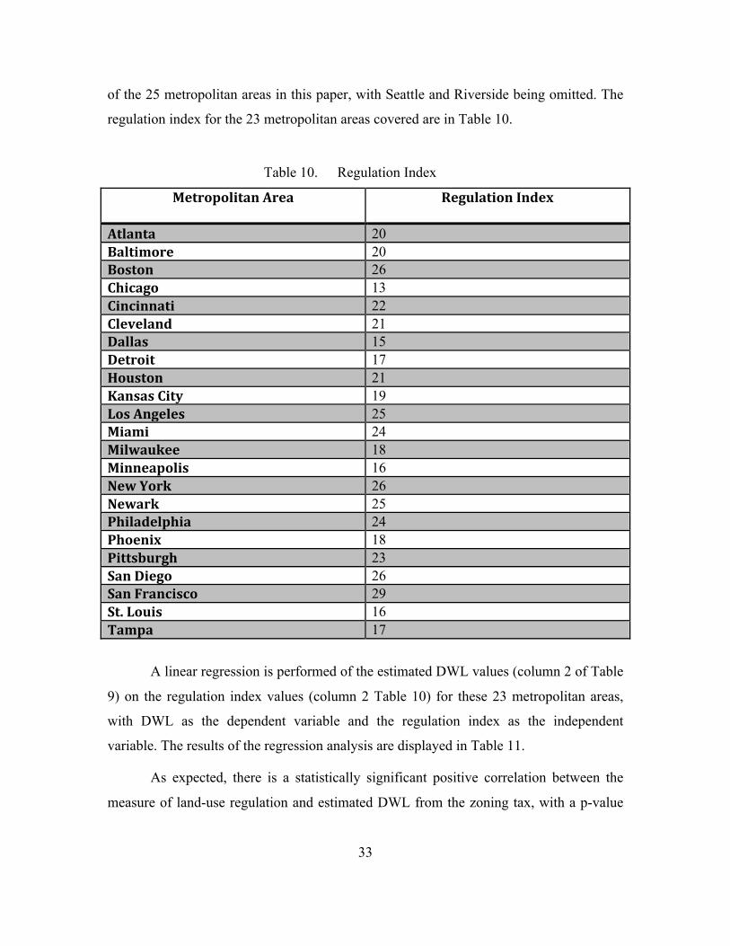
of the 25 metropolitan areas in this paper, with Seattle and Riverside being omitted. The

regulation index for the 23 metropolitan areas covered are in Table 10.

Table 10. Regulation Index

Metropolitan Area

Regulation Index

Atlanta 20 Baltimore 20 Boston 26 Chicago 13 Cincinnati 22 Cleveland 21 Dallas 15 Detroit 17 Houston 21 Kansas City 19 Los Angeles 25 Miami 24 Milwaukee 18 Minneapolis 16 New York 26 Newark 25 Philadelphia 24 Phoenix 18 Pittsburgh 23 San Diego 26 San Francisco 29 St. Louis 16 Tampa 17

A linear regression is performed of the estimated DWL values (column 2 of Table

9) on the regulation index values (column 2 Table 10) for these 23 metropolitan areas,

with DWL as the dependent variable and the regulation index as the independent

variable. The results of the regression analysis are displayed in Table 11.

As expected, there is a statistically significant positive correlation between the

measure of land-use regulation and estimated DWL from the zoning tax, with a p-value

34

of .00154 and R2 of .3864. According to this model, an increase of 1 unit in the regulation

index will result in an increase of approximately $3.0 Billion in DWL.

The correlation between the land-use regulation index created by Malpezzi (1996)

and the measure of DWL calculated in this paper adds additional weight to the theory that

zoning restrictions are the primary driver of housing supply constraints and high housing

prices in many metropolitan areas.

Table 11. Linear Regression of DWL on Regulation Index

Regression Statistics Intercept -‐50,491,273,473.1703 Regulation Index Coefficient 2,998,811,860.8232 R 0.6216 R2 0.3864 Standard Error 1.64897E+10 N 23 Significance level (α) .05 p-‐value 0.00154

35

IV. NET EFFECT ON BAH RATES

A. BAH METHODOLOGY

The Defense Travel Management Office (DTMO) calculates Basic Allowance for

Housing (BAH) rates annually for 364 Military Housing Areas (MHAs). The three

components of the BAH rate calculation are median market rent, average utilities, and

average renter’s insurance (Primer on BAH, 2013). The data used to determine median

rent are collected from multiple sources, including real estate rental listings, real estate

management companies, real estate professionals, and base housing offices. Data are

collected for apartments, townhouses, and single-family houses. Each rank is tied to a

specific type of housing unit, which varies based on dependent status. “With dependents”

means the service member is married or has a dependent child. Having dependents

entitles the service member to a higher BAH rate. The BAH rate for the rank of O-3 with

dependents, which uses the average market rent for a 3-bedroom detached single-family

house, is used as the baseline BAH rate in this paper (Primer on BAH, 2013). The data

for utilities are gathered from the American Community Survey (ACS), while the average

cost of renter’s insurance is determined using data from major insurance companies

(Primer on BAH, 2013).

DTMO provides a BAH component breakdown for each MHA. The percentage

breakdown for rent, utilities, and insurance is calculated as an average value across all

ranks. Median rent makes up the majority of the BAH rate calculation. For the 364

MHAs in 2012 it averaged 75.9%, with a low of 61% and a high of 91% (BAH

Component Breakdown, 2012).

In 2012, total BAH outlays were approximately $19 Billion for the Department

of Defense (DOD), not including supplemental appropriations or Overseas Contingency

Operations (OCO) funding (Air Force Fiscal Year 2012 Budget Estimate, 2011; Army

Fiscal Year 2012 Budget Estimate, 2011; Department of the Navy Fiscal Year 2012

President’s Budget, 2011). BAH outlays were for active duty service members in the

Navy, Marine Corps, Army, and Air Force. BAH obligations comprise approximately

36

13% of the DOD’s military personnel costs (National Defense Budget Estimates, 2013).

This is a significant budget obligation that is directly influenced by rent and, ultimately,

housing prices.

Rent and house prices are highly correlated. This comes as no surprise because

theoretically the price of a house should be the present value of all future rental income

minus expenses. The rent-price ratio is the primary metric used to measure the

relationship between house prices and rent. The rent-price ratio is simply the average

annual rent divided by median house price. Historically, this ratio has remained

remarkably constant, averaging approximately 5% (Davis et al., 2008). Between 1960

and 1995, the rent-price ratio varied only from 4.8% to 6%. During this same period,

house prices and rents increased in real terms at approximately the same rate (Davis et

al., 2008). However, after 1995 the rate began a sharp decline, bottoming out in 2006 at

approximately 3.5%. This unprecedented decline in the rent-price ratio from 1996 to

2006 happened concurrently with an extraordinary rise in housing prices across the U.S.,

leading many to believe there was a housing bubble (Shiller, 2005). Between 2006 and

2012 the rent-price ratio climbed back to its historical level of 5% (Gross Rent-Price

Ratio, 2014). This reversion to the historical mean confirms the importance of the rent-

price ratio as a valuable metric and the close correlation between house prices and rent.

B. CALCULATION OF BAH RATES WITHOUT ZONING TAX

Any reduction in the price of housing will result in a proportional decrease in rent

over the long run. BAH rates for the rank of O-3 with dependents in each metropolitan

area is displayed in column 3 of Table 12. A linear regression analysis of the 2012 BAH

rate on the 2012 Median House Price (PI) is performed. The results are displayed in Table

14. The results show a statistically significant strong positive correlation between BAH

and median house price. This outcome reinforces the high correlation between rent and

house prices because rent makes up the majority of the BAH rate.

The percentage of BAH that is comprised of median rent is provided in column 5

of Table 12. To calculate the decrease in BAH resulting from a 100% reduction to the

zoning tax, the calculated implicit zoning tax percentage from Table 3 is multiplied by

37

rent as a percent of BAH (column 5, Table 12) and the BAH rate (column 3, Table 12).

The result is subtracted from the BAH rate to yield the BAH rate with a 100% zoning tax

reduction. These values are displayed in column 4 of Table 13. Calculations for the BAH

rate with a 75% and a 50% reduction to the zoning tax are also calculated by adjusting

the implicit zoning tax percentage accordingly. These values are in columns 5 and 6 of

Table 13, respectively.

The results show significant decreases in many high-cost areas. San Diego, which

has a large military population due to numerous Navy and Marine Corps bases, shows an

estimated BAH reduction of 47% with a complete elimination of the zoning tax. While a

100% reduction of the zoning tax is likely to be politically infeasible, as discussed earlier,

these results are still valuable because they show the significant decreases to both rent

prices and government spending on BAH entitlements that are possible from zoning

regulation reform. A more reasonable reduction to the zoning tax of 50% still yields an

estimated 24% decrease to the BAH rate in San Diego.

38

Table 12. BAH Rates

Metropolitan Area

Median House Price

(2012 ACS) (PI)

2012 BAH Rate (O-‐3 with

dependents)

Implicit Zoning Tax Percent

Rent as a % of BAH Rate

Atlanta $160,800 $1,470 34.08% 75% Baltimore $271,100 $2,238 26.65% 80% Boston $356,500 $2,913 50.69% 82% Chicago $215,100 $2,031 33.17% 81% Cincinnati $151,800 $1,449 9.61% 74% Cleveland $139,400 $1,452 16.35% 75% Dallas $158,200 $1,782 23.58% 77% Detroit $77,200 $1,773 19.22% 78% Houston $141,400 $1,995 9.19% 81% Kansas City $156,000 $1,416 -‐0.28% 76% Los Angeles $399,500 $2,625 51.24% 89% Miami $181,500 $2,190 36.31% 83% Milwaukee $192,900 $1,560 8.92% 76% Minneapolis $203,700 $1,872 20.03% 82% New York $450,300 $3,027 44.21% 81% Newark $356,700 $2,550 47.49% 77% Philadelphia $244,000 $2,253 17.40% 77% Phoenix $156,100 $1,611 24.55% 79% Pittsburgh $124,300 $1,929 0.50% 79% Riverside $214,100 $1,914 20.91% 86% San Diego $386,400 $2,316 53.48% 88% San Francisco $719,800 $3,015 70.94% 91% Seattle $325,200 $2,049 56.67% 82% St. Louis $155,200 $1,653 0.52% 76% Tampa $132,400 $1,989 3.91% 80%

39

Table 13. BAH Rates with Zoning Tax Reduction

Metropolitan Area

Median House Price (2012 ACS)

(PI)

2012 BAH Rate

(O-‐3 with dependents)

BAH Rate w/ 100% Zoning Tax

Reduction


Reduction


Reduction Atlanta $160,800 $1,470 $1,094 $1,188 $1,282 Baltimore $271,100 $2,238 $1,761 $1,880 $1,999 Boston $356,500 $2,913 $1,702 $2,005 $2,308 Chicago $215,100 $2,031 $1,485 $1,622 $1,758 Cincinnati $151,800 $1,449 $1,346 $1,372 $1,397 Cleveland $139,400 $1,452 $1,274 $1,318 $1,363 Dallas $158,200 $1,782 $1,458 $1,539 $1,620 Detroit $77,200 $1,773 $1,507 $1,574 $1,640 Houston $141,400 $1,995 $1,847 $1,884 $1,921 Kansas City $156,000 $1,416 $1,419 $1,418 $1,417 Los Angeles $399,500 $2,625 $1,428 $1,727 $2,026 Miami $181,500 $2,190 $1,530 $1,695 $1,860 Milwaukee $192,900 $1,560 $1,454 $1,481 $1,507 Minneapolis $203,700 $1,872 $1,564 $1,641 $1,718 New York $450,300 $3,027 $1,943 $2,214 $2,485 Newark $356,700 $2,550 $1,618 $1,851 $2,084 Philadelphia $244,000 $2,253 $1,951 $2,027 $2,102 Phoenix $156,100 $1,611 $1,299 $1,377 $1,455 Pittsburgh $124,300 $1,929 $1,921 $1,923 $1,925 Riverside $214,100 $1,914 $1,570 $1,656 $1,742 San Diego $386,400 $2,316 $1,226 $1,499 $1,771 San Francisco $719,800 $3,015 $1,069 $1,555 $2,042 Seattle $325,200 $2,049 $1,097 $1,335 $1,573 St. Louis $155,200 $1,653 $1,646 $1,648 $1,650 Tampa $132,400 $1,989 $1,927 $1,942 $1,958

40

Table 14. Linear Regression of BAH Rate on PI

Regression Statistics Intercept 1349.1160 PI Coefficient 0.0029 R 0.83165 R2 0.69164 Standard Error 275.09985 N 25 Significance level (α) .05 p-‐value 2.59E-‐07

41

V. CONCLUSION

While the calculations in this paper are suggestive, the results show the significant

cost imposed by zoning regulation. The net loss to society for the benefit of incumbent

homeowners is particularly severe in the high-cost markets. The unrealized potential that

exists is significant if the burden of the zoning tax can be lifted or eased, even by a small

amount. Local governments can address negative externalities from land development in

more efficient ways, such as infrastructure development. These externalities can also be

internalized through private bargaining via covenants and homeowner associations

(HOAs), as opposed to coerced regulation.

Why do nearly all zoning regulations and other land-use restrictions favor single-

family homes and existing homeowners above all else? Fischel (2004) believes it began

with a shift in judicial preferences during the early 20th century, favoring single-family

homes as representing American ideals. In the 1970s the power of existing suburban

homeowners increased due to a transition toward even more burdensome and restrictive

land-use regulations throughout the country (Quigley & Rosenthal, 2005). The primary

reason for the continuation of such onerous land-use restrictions in so many metropolitan

areas is likely the concentrated benefits they provide to the existing local homeowners,

while the significant costs are dispersed primarily to renters and budding home buyers.

Reducing zoning regulation will lower housing costs, increase homeownership in

a sustainable and permanent way, and result in real economic growth. This significant net

benefit to society should not be abdicated to the interests of one group.

42


43

LIST OF REFERENCES

Cappel, A. J. (1991). A walk along willow: patterns of land use coordination in pre-zoning New Haven (1870–1926). Yale Law Journal, 101(3), 617–642.

Davis, M. A., Lehnert, A., & Martin, R. F. (2008). The rent-price ratio for the aggregate stock of owner-occupied housing. Review of Income and Wealth, 54(2), 279-284.

Deakin, E. (1989). Growth controls and growth management: a summary and review of empirical research. In D. J. Brower, D. R. Godschalk, & D. R. Porter (Eds.), Understanding growth management: Critical issues and a research agenda. Washington, DC: The Urban Land Institute.

Defense Travel Management Office. (2012). Basic allowance for housing component breakdown. Retrieved from http://www.defensetravel.dod.mil/site/bah.cfm

Defense Travel Management Office. (2012). 2012 BAH rates – with dependents. Retrieved from http://www.defensetravel.dod.mil/site/bah.cfm

Defense Travel Management Office. (2013). A primer on the basic allowance for housing (BAH) for the uniformed services. Retrieved from http://www.defensetravel.dod.mil/Docs/perdiem/BAH-Primer.pdf

Department of the Air Force. (2011). Fiscal year 2012 budget estimates: Military personnel appropriation. Retrieved from http://www.saffm.hq.af.mil/budget/pbfy12.asp

Department of the Army. (2011). Fiscal year 2012 budget estimates: Military personnel justification book. Retrieved from http://asafm.army.mil/offices/BU/BudgetMat.aspx?OfficeCode=1200

Department of the Navy. (2011). Fiscal year 2012 president’s budget. Retrieved from http://www.finance.hq.navy.mil/FMB/12pres/DON_PB12_Press_Brief.pdf

Ellickson, R. C. (1977). Suburban growth controls: An economic and legal analysis. The Yale Law Journal, 86(3), 385-511.

Fischel, W. A. (2004). An economic history of zoning and a cure for its exclusionary effects. Urban Studies, 41(2), 317-340.

Follain, J. R. (1979). The price elasticity of the long-run supply of new housing construction. Land Economics, 55(2), 190-199.

Glaeser, E., & Gyourko, J. (2002). The impact of zoning on housing affordability. National Bureau of Economic Research, Working Paper 8835.

44

Glaeser, E., Gyourko, J., & Saks, R. (2003). Why is Manhattan so expensive? Regulation and the rise in house prices. National Bureau of Economic Research, Working Paper 10124.

Glaeser, E., Gyourko, J., & Saks, R. (2005). Why have housing prices gone up? National Bureau of Economic Research, Working Paper 11129.

Glaeser, E., Gyourko, J., & Saiz, A. (2008). Housing supply and housing bubbles. Journal of Urban Economics, 64, 198-217.

Green, R. K., Malpezzi, S., & Mayo, S. K. (2005). Metropolitan-specific estimates of the price elasticity of supply of housing, and their sources. The American Economic Review, 95(2), 334-339.

Hanushek, E. A. & Quigley, J. M. (1980). What is the price elasticity of housing demand? The Review of Economics and Statistics, 62(3), 449-454.

Lincoln Institute of Land Policy. (2014). Gross rent-price ratio, U.S. stock of owner-occupied housing, 1960-2014. Retrieved from http://www.lincolninst.edu/subcenters/land-values/rent-price-ratio.asp

Malpezzi, S. (1996). Housing prices, externalities, and regulation in U.S. metropolitan areas. Journal of Housing Research, 7(2), 209-41.

Muth, R. F. (1960). The demand for non-farm housing. In A. C. Harberger (Ed.), The Demand for Durable Goods (pp. 29-75). Chicago: University of Chicago Press.

Muth, R. F. (1971). The derived demand for urban residential land. Urban Studies, 8, 243-254.

National Association of Home Builders. (2014). NAHB compilation of 2012 American Community Survey summary files. Retrieved from http://www.nahb.org/

Office of the Under Secretary of Defense (Comptroller). (2013). National defense budget estimates for fiscal year 2014. Retrieved from http://comptroller.defense.gov

Polinsky, A. M. & Ellwood, D. T. (1979). An empirical reconciliation of micro and grouped estimates of the demand for housing. The Review of Economics and Statistics, 61(2), 199-205.

Quigley, J. M., & Rosenthal, L. A. (2005). The effects of land use regulation on the price of housing: What do we know? What can we learn? Cityscape: A Journal of Policy Development and Research, 8(1), 69-137.

Shiller, R. (2005). Irrational exuberance. Princeton, NJ: Princeton University Press.

45

United States Air Force. (2011). Fiscal year 2012 budget overview. Retrieved from http://www.saffm.hq.af.mil/budget/pbfy12.asp

United States Army. (2011). Army fiscal year 2012 budget overview. Retrieved from http://asafm.army.mil/offices/BU/BudgetMat.aspx?OfficeCode=1200

United States Census Bureau. (2012). American Community Survey. Available from https://www.census.gov/housing

46


47

INITIAL DISTRIBUTION LIST

1. Defense Technical Information Center Ft. Belvoir, Virginia 2. Dudley Knox Library Naval Postgraduate School Monterey, California

NAVAL POSTGRADUATE SCHOOL - Defense … · iii Approved for public release; distribution is...

Documents

Transcript of NAVAL POSTGRADUATE SCHOOL - Defense … · iii Approved for public release; distribution is...