NATIONAL INSTITUTE OF TECHNOLOGY - …arajasekhar.weebly.com/uploads/2/2/5/7/22576192/thesis.pdfAN...

AN INTELLIGENT DESIGN OF DAMPING CONTROLLERS

FOR DYNAMIC STABILITY ENHANCEMENT OF SINGLE

MACHINE INFINITE BUS SYSTEM WITH TCSC AND UPFC

CONTROLLERS: ARTIFICIAL BEE COLONY APPROACH

SUBMITTED TO THE FACULTY OF ENGINEERING

A DISSERTATION

NATIONAL INSTITUTE OF TECHNOLOGY, WARANGAL, A.P.

IN PARTIAL FULFILLMENT OF THE REQUIREMENTS

FOR THE AWARD OF THE DEGREE OF

BACHELOR OF TECHNOLOGY

IN

ELECTRICAL AND ELECTRONICS ENGINEERING

By

Under the esteemed guidance of Asst. Prof. Y. Chandrasekhar

DEPARTMENT OF ELECTRICAL ENGINEERING

NATIONAL INSTITUTE OF TECHNOLOGY

(An Institution of National Importance)

WARANGAL (A. P.)-506004

2009-2013

Mr. Bagepalli Sreenivas Teja (EE09283)

Mr. Anguluri Rajasekhar (EE08210)

Mr. K Vamsi Krishna (EE08242)

CERTIFICATE

This is to certify that the dissertation work entitled “AN INTELLIGENT DESIGN OF

DAMPING CONTROLLERS FOR DYNAMIC STABILITY ENHANCEMENT OF

SINGLE MACHINE INFINITE BUS SYSTEM WITH TCSC AND UPFC

CONTROLLERS: ARTIFICIAL BEE COLONY APPROACH” is a bonafide work

carried out by Mr. B. Sreenivas Teja (Roll No. EE09283), Mr. A. Rajasekhar (Roll No.

EE08210) & Mr. K Vamsi Krishna (Roll No. EE08242) towards the partial fulfillment of the

requirements for the award of the degree of Bachelor of Technology in Electrical and

Electronics Engineering from National Institute of Technology, Warangal during the year

2012-2013.

DEPARTMENT OF ELECTRICAL ENGINEERING

NATIONAL INSTITUTE OF TECHNOLOGY

WARANGAL (A.P)-506004

Deemed University

2012-2013

Project Guide

Mr. Y. Chandrasekhar,

Assistant Professor,

Dept. of Electrical Engineering,

National Institute of Technology,

Warangal-506004.

Head of the Department

Dr. N. Subrahmanyam,

Professor and Head,

Dept. of Electrical Engineering,

National Institute of Technology,

Warangal-506004.

ACKNOWLEDGEMENTS

We would like to express our deepest gratitude to our thesis supervisor Shri.

Y. Chandrasekhar, Assistant Professor, Electrical Engineering Department,

National Institute of technology, Warangal, for his valuable guidance and

advices in the successful completion of this dissertation work. We are very

much indebted to him for suggesting this topic and his encouragement without

which it would not have been possible to complete our work successfully.

We would also like to take this opportunity to express our profound thanks to

Dr. N. SUBRAMANYAM, Professor and Head of Electrical Engineering

Department for his cooperation throughout this work and efforts for arranging

this dissertation work.

We are thankful to the faculty of Electrical Engineering Department for their

active support and also their cooperation in collection of relevant data regarding

this topic. Also, we wish to thank all those pioneering researchers and their

outstanding contributions towards this topic. It couldn’t have been possible

without their ground work.

Finally, we wish to express our profound gratitude to our beloved parents,

other family members and all of our friends for providing constant

encouragement throughout this dissertation work.

B. Sreenivas Teja (Roll No. EE09283)

A. Rajasekhar (Roll No. EE08210)

K Vamsi Krishna (Roll No. EE08242)

ABSTRACT

In this dissertation an attempt has been made in designing novel and intelligent

flexible AC transmission system (FACTS) devices such as Thyristor Controlled Series

Compensator (TCSC), unified power flow controller (UPFC) and their coordinated

design based on PID controller for a Single Machine Infinite Bus (SMIB). To carry

out small signal stability studies with the proposed method, a SMIB linear model of

Philip-Heffron model, a well-known model for synchronous generator has been

considered. Recent past has witnessed the advancements of Power System Stabilizers

(PSS) and their variants for enhancing the stability of power system. But the added

advantages of FACTS based design outperformed PSS in terms of performance and

implementation perspective. Though FACTS based controllers are proved to be well

suited for modern day power systems, to get better performances the unknown

parameters of these devices has to be tuned optimally. To handle this problem this

dissertation puts forward an approach as an alternative for present day’s practice of

designing controllers, where traditional methods like classical optimization, manual

tuning methods are preferred. A single objective optimization frame work based on

time integral indices has been developed for obtaining optimum parametric gains of

the controllers. Further a swarm intelligent based Artificial Bee Colony (ABC)

algorithm is considered to carry out this optimization task. Various loading conditions

are considered for different combinations of TCSC, UPFC, PID, PSS and a detailed

analysis is carried out. Computer simulations and extensive analysis followed by

several comparisons with reported results (in literature) revealed the superiority of

proposed intelligent method in designing state-of-art FACTS controllers for a SMIB

system. An Industrial Standard MATLAB/SIMULINK simulation package is used to

simulate the system considered.

Keywords: AVR; PSS; UPFC; TCSC; Modified Philip-Heffron’s Model; SMIB;

Artificial Bee Colony Algorithm; Global Optimization.

INDEX

Chapter.

No CONTENTS

Page

No.

List of Figures

List of Tables

i

iii

1 INTRODUCTION

1.1. Automatic Voltage Regular (AVR) & Power System Stabilizer

(PSS)

1.2. Modified Philip-Heffron’s Model

1.3. Flexible AC Transmission Systems (FACTS devices)

1.3.1. Thyristor Controlled Series Compensator (TCSC)

1.3.2. Unified Power Flow Controller (UPFC)

1.3.3. Coordinated Design of PID, PSS & FACTS Controllers

1.4. Literature Survey

1.5. Artificial Bee Colony methods for Engineering Applications

1.6. Organization of Report

1

3

3

4

5

5

6

7

7

2 Power System Modeling

2.1. Modified Philip-Heffron’s Model for SMIB system

2.1.1. Generator Modeling

2.1.2. Linearized Model of Philip-Heffron’s Model

2.1.3. PSS & Excitation System

2.2. Modeling of SMIB power system with TCSC Controller

2.2.1. Generator Modeling

2.2.2. Thyristor Controlled Series Compensator Modeling

2.2.3. TCSC Controllers


2.3.Modeling of SMIB power system with UPFC Controller

2.3.1. Unified Power Flow Controller (UPFC)

2.3.2. Non-linear Dynamic Model

2.3.3. Linear Dynamic Model


2.3.5. UPFC Damping Controllers

8

8

9

12

13

13

16

16

17

18

18

19

21

23

24

3 Problem Formulation

3.1. Modified Philip-Heffron’s Model

3.1.1. Structure of PSS

3.1.2. PID-PSS based Controllers

3.1.3. Time domain based Objective Function

3.2. Single Machine Infinite Bus System with TCSC Controller

3.2.1. TCSC Controller

3.2.2. PI based PSS & TCSC Controller


3.3. Single Machine Infinite Bus System with UPFC Controller

3.3.1. Structure of UPFC damping controller

3.3.2. PI based UPFC damping Controllers


25

25

25

26

27

27

27

28

29

29

29

30

4 Artificial Bee Colony Algorithm

4.1. Biological Motivation

4.2. The Algorithm

32

33

5 Experimental Section

5.1. System parameters of SMIB System considered for M P-H Model

5.2. System parameters of SMIB System with TCSC Controller

5.3. System parameters of SMIB System with UPFC Controller

5.4. Parameters of ABC Algorithm

39

39

40

40

6 Simulations & Results

6.1. PID-PSS Controller using Modified Philip-Heffron’s Model for

SMIB System

6.2. Coordinated tuned PI Controller and TCSC-PSS for SMIB

System using ABC algorithm

6.3. Coordinated tuned PI Controller and UPFC damping controllers

for SMIB System using ABC algorithm

42

50

57

Conclusions & Scope of Future Research 68

List of Publications From this Dissertation 69

Appendix 70

REFERENCES 74

List of figures

Figure

No.

Figure about

Chapter

No.

Page

No.

1.1

2.1

2.2

2.3

2.4

2.5

2.6

2.7

2.8

2.9

2.10

2.11

2.12

2.13

3.1

3.2

3.3

3.4

6.1

6.2

6.3

6.4

6.5

6.6

6.7

6.8

6.9

6.10

6.11

6.12

6.13

6.14

6.15

6.16

6.17

6.18

6.19

6.20

Graphical representation of AVR and PSS damping phenomenon

Single machine power system model

Modified Philip-Heffron’s model

Structure of PSS and IEEE- ST1A

Single machine infinite bus power system with TCSC

Phillips-Heffron model of SMIB with TCSC and PSS

Structure of TCSC controller

Structure of PSS and IEEE Type-ST1A Excitation system

Single machine infinite bus power system with UPFC

Phasor diagram showing the modulation of real power flow

through bus voltage magnitude and phase regulation.

Linear Philip-Heffron model of SMIB power system with UPFC

IEEE type - ST1 excitation system with PSS

Structure of Lead-lag UPFC controller (mB, mE, δB)

Structure of δE Lead-lag controller with DC voltage regulator

Structure of Lead-lag PSS with PID controller

Structure of TCSC controller

Structure of TCSC controller and PSS with PI controller

Structure of PI controller based mB, δE or δB damping controllers

Speed deviation for a step change of 10% in Vref for heavy loaded

or strong system

Rotor angle deviation for a step change of 10% in Vref for strong

system

Speed dev. for a step change of 10% in Vref for weak system

Rotor angle dev. for a step change of 10% in Vref for weak system

Speed dev. for a step change of 10% in Vref for nominal

Rotor angle dev. for a step change of 10% in Vref for nominal

system

Convergence Characteristics of ABC towards optimum for

different loading conditions without PID

Convergence Characteristics of ABC towards optimum for

different loading conditions with PID

Speed deviation response for Heavy loaded system

Rotor angle deviation response for Heavy loaded system

Speed deviation response for Light loaded system

Rotor Angle Deviation: Light loaded

Speed Deviation: Nominal loaded

Rotor Angle Deviation: Nominal loaded

Convergence of ABC towards minimum: without PI Controller

Convergence of ABC towards minimum: with PI Controller

Speed deviation response of Nominal loaded system

Rotor angle deviation response of Nominal loaded system

Speed deviation response of Light loaded system

Rotor angle deviation response of light loaded system

1

2

2

2

2

2

2

2

2

2

2

2

2

2

3

3

3

3

6

6

6

6

6

6

6

6

6

6

6

6

6

6

6

6

6

6

6

2

8

11

12

13

15

17

17

18

19

23

23

24

24

26

27

28

30

44

44

45

46

46

47

48

48

51

52

52

53

54

54

55

55

61

63

63

i

6.21

6.22

6.23

6.24

6.25

C.1

C.2

C.3

Speed deviation response of heavy loaded system

Rotor angle deviation of Heavy loaded system

Objective function minimization plot for heavy loaded system

Objective function minimization plot for nominal loaded system

Objective function minimization plot for light loaded system

Linear Philip-Heffron’s model of SMIB employing PI based

UPFC Damping Controllers

Linear Philip-Heffron’s model of SMIB employing PI Controllers

for TCSC and PSS

Modified Philip-Heffron’s Model of SMIB with PID-PSS

6

6

6

6

6

65

65

66

66

67

72

72

73

ii

List of Tables

Figure

No.

Figure about

Chapter

No.

Page

No.

5.4.1

6.1.1

6.1.2

6.1.3

6.1.4

6.1.5

6.2.1

6.2.2

6.2.3

6.2.4

6.3.1

6.3.2

6.3.3

6.3.4

6.3.5

6.3.6

6.3.7

6.3.8

6.3.9

6.3.10

Algorithmic Parameters (ABC)

Loading conditions considered (p.u)

Parametric Values Obtained for PSS Using ABC

Parametric Values Obtained for PID Using ABC

Mean and Standard Deviation (std) without and with PID

controller

Settling times and peak values for various loading conditions

Parametric Values Obtained for Coordinated TCSC-PSS Using

ABC and Obj Fun Minimization values

Parametric Values Obtained for coordinated PI controller TCSC-

PSS Using ABC and obj func. Minimization values

Peak values for various loading conditions

Settling time values for various loading conditions

Loading conditions considered (p.u)

Parametric values of damping controllers obtained for Nominal

loaded system using ABC

Parametric values of coordinated PI controllers obtained for

nominal loaded system using ABC

Parametric values of damping controllers obtained for light loaded

system using ABC

Parametric values of coordinated PI controllers obtained for light

loaded system using ABC

Parametric values of PI controllers obtained for heavy loaded

system using ABC

Parametric values of coordinated tuned PI controllers obtained for

heavy loaded system using ABC

Time domain indices for speed and rotor angle deviation responses

and objective function minimization values for nominal loaded

system


and objective function minimization values for light loaded system


and objective function minimization values for heavy loaded

system

5

6

6

6

6

6

6

6

6

6

6

6

6

6

6

6

6

6

6

6

41

42

42

43

43

49

50

51

56

56

57

57

58

58

58

59

59

60

62

64

iii

1

CHAPTER 1

INTRODUCTION

1.1 Automatic Voltage Regulator (AVR) & Power System Stabilizer (PSS)

In the earlier days, the power systems were simple and relatively non-remote. To supply the

load demand in earlier days, power was generated beside the load center locally. In the recent

years the complexity of power system has been drastically increased with the rapid growth of

power demand. Due to limited availability of resources and other environmental constraints

modern day power systems are getting more loaded than before causing system to operate near

their transient stability limits. Power system is dynamic and nonlinear system, often experience

changes in generation, transmission and loading conditions. For reliable power supply, the

modern day power systems require continuous balance between electrical power generation and

varying load demand.

As the distantly located interconnected power systems need to be maintained at constant

operating voltage, fast acting high gain Automatic Voltage Regulators (AVR) are being used for

synchronous generators. A high response exciter is beneficial in increasing the synchronizing

torque, thus enhancing the transient stability i.e. to hold the generator in synchronism with power

system during large transient fault condition. Though AVRs are used to maintain constant

voltage, they are responsible for low frequency oscillations (0.1-3 Hz) and causes negative

damping on the rotor by producing a component of electric torque out of phase with speed

deviation () [2].Stability of synchronous generators depends upon number of factors such as

setting of Automatic Voltage Regulators (AVR). AVR and generator field dynamics introduces a

phase lag so that resulting torque is out of phase with both rotor angle and speed deviation.

Positive synchronizing torque and negative damping torque often result, which can cancel the

small inherent positive damping torque available, leading to instability. Furthermore if not

sufficiently damped, these oscillations may keep grow in magnitude until loss of synchronism

results. This will affects the small signal stability of power system. Small signal stability refers to

the ability to maintain synchronism under small disturbances, which are generally caused by

small variations in loads and generation.

2

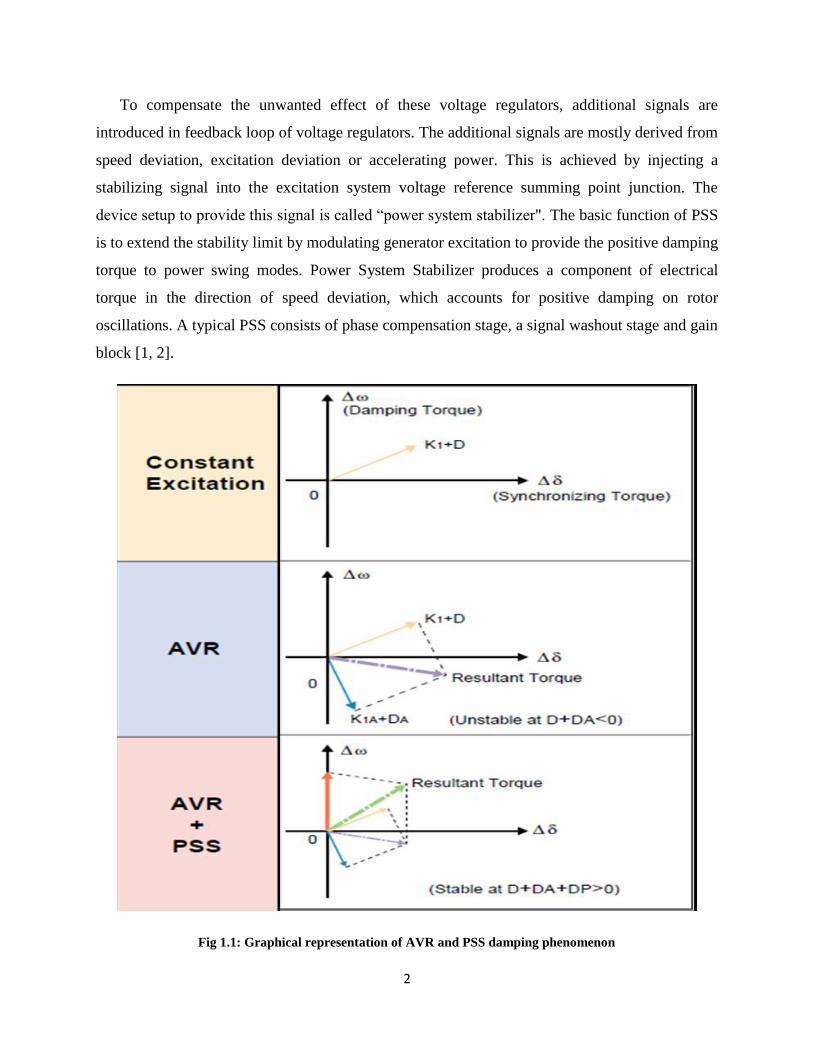
To compensate the unwanted effect of these voltage regulators, additional signals are

introduced in feedback loop of voltage regulators. The additional signals are mostly derived from

speed deviation, excitation deviation or accelerating power. This is achieved by injecting a

stabilizing signal into the excitation system voltage reference summing point junction. The

device setup to provide this signal is called ―power system stabilizer". The basic function of PSS

is to extend the stability limit by modulating generator excitation to provide the positive damping

torque to power swing modes. Power System Stabilizer produces a component of electrical

torque in the direction of speed deviation, which accounts for positive damping on rotor

oscillations. A typical PSS consists of phase compensation stage, a signal washout stage and gain

block [1, 2].

Fig 1.1: Graphical representation of AVR and PSS damping phenomenon

3

1.2 Modified Philip-Heffron’s Model

To carry the small signal stability studies of Single Machine Infinite Bus (SMIB) linear

model of Philip-Heffron, which is well known model for synchronous generators is considered.

It is quite accurate for the small signal stability studies of power systems [11]. It has worked

successfully for the designing and tuning of conventional power system stabilizers. Though these

stabilizers have simple robust structures, tuning them not only requires considerable expertise

but also a knowledge of system parameters external to the generating station. These parameters

may vary during normal operation. of the power system. Even in the case of single machine

infinite bus models, estimates of equivalent line impedance and the voltage of the remote bus are

required. The PSS design also requires information of the rotor angle δ measured with respect to

the remote bus. These parameters cannot be measured directly and hence they are to be estimated

based on reduced order models of the rest of the system connected to the generator. If the

available information for the rest of the system is inaccurate, the conventionally designed PSS

may result in poor system performance.

Recently Gurrala and Sen [3] proposed a modified Philip-Heffron model with PSS which

judges system disturbances like change in system configuration and load changes based on

deviation of power flow, voltage and rotor angle at secondary of step-up transformer. The main

advantage with this system is that it doesn‘t require knowledge of system parameters external to

generating station which may vary during normal operation. The PSS tries to control the rotor

angle measured with respect to the local bus rather than the angle δ measured with respect to the

remote bus to damp the oscillations. All PSS design parameters are thus calculated from local

measurements and there is no need to estimate or compute the values of equivalent external

impedances, bus voltage and rotor angles at the remote bus.

1.3 Flexible AC Transmission Systems (FACTS devices)

The most widely used conventional PSS is lead-lag PSS where the gain settings are fixed

under certain value which are determined under particular operating conditions to result in

optimal performance for a specific condition. However, they give poor performance under

different synchronous generator loading conditions. But PSS causes variations in voltage profiles

4

and its operating time is relatively high. When it is not properly tuned, PSS may lead to leading

power factor operations [8-10].

Due to advancement in Power Electronic Drive technologies, Flexible AC Transmission

Systems (FACTS) devices have been economically proved to be very useful for enhancement of

power system stability and power transfer capacity, decreasing line losses and generation costs

ameliorates security of power system. FACTS controllers are capable of controlling the network

condition in a very fast manner and this feature of FACTS can be exploited to improve the

stability of a power system. They are able to provide rapid active and reactive power

compensations to power systems, and therefore can be used to provide voltage support and

power flow control, increase transient stability and improve power oscillation damping. Suitably

located FACTS devices allow more efficient utilization of existing transmission networks.

1.3.1 Thyristor Controlled Series Compensator

Fundamental feature of Thyristor based switching controllers is that speed of response of

passive power system components (C & L) and system mechanical response will get enhanced.

Thyristor Controlled Series Compensator (TCSC) belongs to first generation series FACTS

devices. The problem with these devices is that that it can form a series resonant circuit in series

with the reactance of the transmission line, thus limiting the rating of the TCSC to a range of 20

to 70 % the line reactance. The problem with TCSC is that that it can form a series resonant

circuit in series with the reactance of the transmission line, thus limiting the rating of the TCSC

to a range of 20 to 70 % the line reactance. It is widely useful because of its effectiveness in

solving transient problems and is less expensive. Its flexibility and quickness in adjusting the

reactance of transmission line helps in achieving better utilization of transmission capability,

efficient power flow control, transient stability improvement, power oscillation damping & fault

current location [11, 14-18]. To carry the small signal stability studies of Single Machine Infinite

Bus with TCSC controller, linear model of Philip-Heffron, has been considered. It is well known

model for synchronous generators and is quite accurate for the small signal stability studies of

power systems.

5

1.3.2 Unified Power Flow Controller

Unified Power Flow Controller belongs to the family of second generation FACTS devices.

It was proposed by Gyugil. Independent control on both real and reactive power flows is possible

with UPFC controller. It has the ability to adjust the three control parameters, i.e. the bus

voltage, transmission line reactance and phase angle between two buses, either simultaneously or

independently to control power flow and improve the stability. It can also improve the small

signal stability by the damping of low frequency power system oscillations. A UPFC performs

this through the control of in-phase voltage, quadrature voltage and shunt compensation. Wang

has proposed a modified linear Philip-Heffron‘s model of a power system equipped with UPFC.

He had demonstrated the issues related to the design of damping controller and choice of

parameters of UPFC (mB,mE,δB,δE) to be modulated to achieve desired damping [7-9, 19-22].

1.3.3 Coordinated design of POD, PSS and FACTS controllers

It has been observed that utilizing a feedback supplementary control (PSS), in addition to the

FACTS-device primary control, can considerably improve system damping and can also improve

system voltage profile, which is advantageous over PSSs. However, possible interaction between

PSSs and FACTS-based stabilizers may deteriorate much of their contributions to, and may even

cause adverse effect on, damping of system oscillations. Therefore, coordinated design between

PSSs and FACTS-based stabilizers is a necessity, both to make use of the advantages of the

different stabilizers and to avoid the demerits accompanied with their operations [11].

In addition to that PID controller for Modified Philip-Heffron model based Single Machine

Infinite Bus power system and coordinated tuned PI controllers for both TCSC controller based

SMIB and UPFC based SMIB has been proposed. To obtain parametric values of various

damping controllers, trial and error methods are not suitable and also to avoid the destabilizing

interactions the tuning of parameters of different controllers should be coordinated. As the

coordinated approach is more intricate than normal controller design and efficient algorithm

should be developed to get optimal parametric values for various damping controllers for

optimum system performance [15].

For this purpose of designing coordinated damping controllers, we applied new swarm

intelligent based Artificial Bee Colony (ABC) algorithm. ABC algorithm was first proposed by

6

Karaboga and Basturk [24, 25] algorithm for numerical function optimization. Due its simplicity

in structure and also having good global and local exploration skills it had been used in designing

many real world practical problems. In this work we had used ABC in designing damping

controllers for modified Philip-Heffron modeled SMIB, coordinated PI controller based TCSC &

PSS for SMIB and also coordinated PI based UPFC damping controllers for SMIB system.

1.4 Literature Survey

Since the 1960‘s, lead-lag Power System Stabilizers have been used to add damping to

electromechanical oscillations. Larsen and Swann [2] deeply discussed, in a three-part paper, the

general concepts associated with PSSs. In Part I, the concepts of applying and tuning PSSs

utilizing speed, frequency, and power input signals have been described. Part II dealt with the

performance objectives of PSSs. Part III addressed the major practical considerations associated

with applying PSSs. Although the application of GA to synthesize the PSS parameters yielded

promising results, recent research has identified some deficiencies in GA performance. Recently

Gurrala and Sen [3] proposed a modified Philip-Heffron model with PSS which judges system

disturbances like change in system configuration and load changes based on deviation of power

flow, voltage and rotor angle at secondary of step-up transformer. The main advantage with this

system is that it doesn‘t require knowledge of system parameters external to generating station

which may vary during normal operation. As a result, different optimization algorithms, such as

simulated annealing [4], particle swarm [5], Tabu search [6, 7], and evolutionary programming

[54], have been also explored. In 1988, Hingorani [7-9] have initiated the concept of FACTS

devices and their application for the following purposes: control of power routing, loading of

transmission lines near their steady-state, short-time and dynamic limits, reducing generation

reserve margins, and finally, limiting the impact of multiple faults and, hence, containing

cascaded outages. Sidhartha Panda, and N. P. Padhya [10] has proposed an approach to tune the

parameters of a Thyristor Controlled Series Compensator (TCSC) and PSS coordinately using

PSO algorithm to avoid destabilizing interactions. AlAwami, Ali Taleb [11] has investigated the

effectiveness of the coordinated design of power system stabilizers and FACTS-based stabilizers

to improve power system transient stability.

7

1.5 Artificial Bee Colony Methods for Engineering Applications

Out of all existing swarm intelligent algorithms based on bees like BCO, BA, MBO etc.,

Artificial Bee Colony (ABC) algorithm has gained wide reputation in research community

because of its outstanding performance on various kinds of practical problems [26]. Hemamalini

and Simon [27] applied this ABC technique for solving Economic dispatch problem, which

comes under the category of non-smooth cost function; the proposed technique was compared

with GA, PSO and showed that ABC had recorded best feasible solutions. Hemalini and Simon

[28] proposed a new multi-objective artificial bee colony (MOABC) to solve economic/emission

dispatch (EED) problem and also used fuzzy decision theory to extract the best compromise

solution. Omkar et al [29] presented a generic method for multi-objective design optimization of

laminated composite components based on Vector Evaluated Artificial Bee Colony (VEABC)

algorithm which is a parallel vector evaluated type, swarm intelligence multi-objective variant of

ABC. Abu-Mouti and El-Harwary [30] presented a medication in neighboring search of ABC

and applied in determination of optimal size, location and power factor for a distributed

generation (DG) to minimize total power losses on 33-bus and 69-bus feeder systems. Akay and

Karaboga [31] applied ABC in solving Engineering design problems which are generally large

scale or nonlinear or constrained optimization problems just by simply adding a constraint

handling technique into the selection step of ABC. A comprehensive view of recent

developments and real world applications can be found in [32].

1.6 Organization of report

The rest of the report is organized as follows; Chapter 2 deals with the mathematical

modeling of power system for single machine infinite bus system with TCSC and UPFC

controller. Also the linear Modified Philip-Heffron‘s model for single machine infinite bus

system has been described. Chapter 3 describes the problem formulation for designing various

damping controllers for different systems considered followed by the objective function

considered. A chapter 4 brief about the ABC algorithm and it is followed by experimental

section in Chapter 5. The simulations and results are put forth in Section 6 and at end we provide

few conclusions.

8

CHAPTER 2

Power System Modeling

2.1 Modified Philip-Heffron’s model for SMIB system

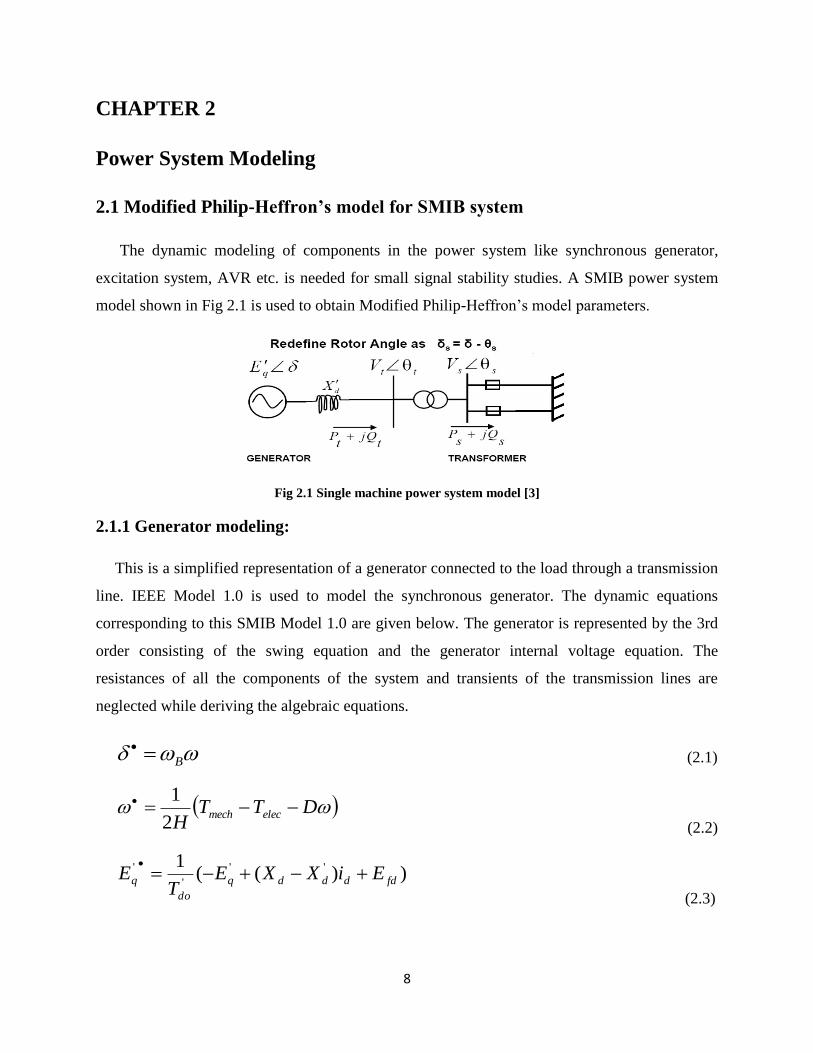
The dynamic modeling of components in the power system like synchronous generator,

excitation system, AVR etc. is needed for small signal stability studies. A SMIB power system

model shown in Fig 2.1 is used to obtain Modified Philip-Heffron‘s model parameters.

Fig 2.1 Single machine power system model [3]

2.1.1 Generator modeling:

This is a simplified representation of a generator connected to the load through a transmission

line. IEEE Model 1.0 is used to model the synchronous generator. The dynamic equations

corresponding to this SMIB Model 1.0 are given below. The generator is represented by the 3rd

order consisting of the swing equation and the generator internal voltage equation. The

resistances of all the components of the system and transients of the transmission lines are

neglected while deriving the algebraic equations.

B

(2.1)

2

1 DTT

Helecmech

(2.2)

))((1 ''

'

'

fddddq

do

q EiXXET

E

(2.3)

9

)}({1'

tpssrefEfd

e

fd VVVKET

E

(2.4)

)( '''

qdqdqqelec iiXXiET (2.5)

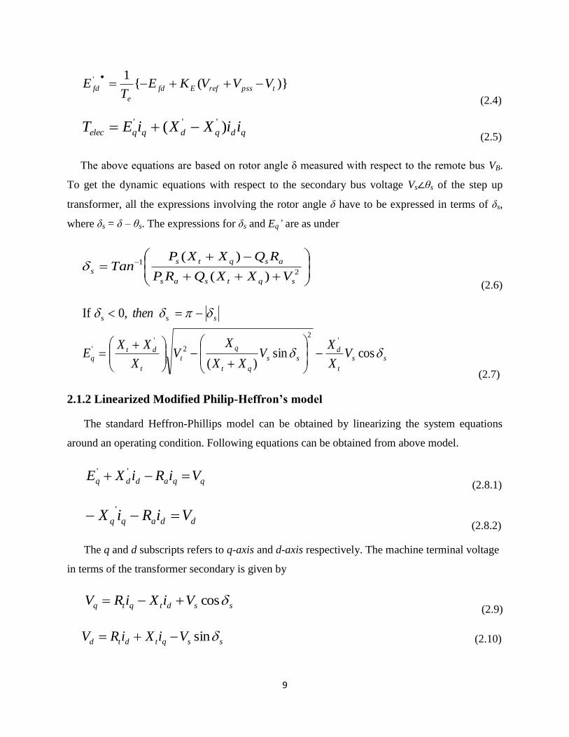
The above equations are based on rotor angle δ measured with respect to the remote bus VB.

To get the dynamic equations with respect to the secondary bus voltage Vs∠θs of the step up

transformer, all the expressions involving the rotor angle δ have to be expressed in terms of δs,

where δs = δ – θs. The expressions for δs and Eq’ are as under

)(

)(2

1

sqtsas

asqts

sVXXQRP

RQXXPTan

(2.6)

cos sin)(

,0 If

'2

2'

'

ss

ss

t

dss

qt

q

t

t

dtq

s

VX

XV

XX

XV

X

XXE

then

(2.7)

2.1.2 Linearized Modified Philip-Heffron’s model

The standard Heffron-Phillips model can be obtained by linearizing the system equations

around an operating condition. Following equations can be obtained from above model.

''

qqaddq ViRiXE (2.8.1)

'

ddaqq ViRiX (2.8.2)

The q and d subscripts refers to q-axis and d-axis respectively. The machine terminal voltage

in terms of the transformer secondary is given by

cos ssdtqtq ViXiRV (2.9)

sin ssqtdtd ViXiRV

(2.10)

10

Substitution of Eqn (2.8) in Eqn (2.9) and Eqn (2.10), and there by rearranging gives the

following matrix

sin-

cos

-

- ''

ss

qss

q

d

tqt

ttd

V

EV

i

i

XXR

RXX

(2.11)

The system mechanical, electrical equations and (2.11) are linearized to obtain K constants as

follows

soso

qt

dq

qt

soqosoV

XX

XX

XX

EVK

sin

cos '

1

(2.12)

;'2 qo

td

tqi

XX

XXK

(2.13)

;'

3

td

dt

XX

XXK

(2.14)

; sin'

'

4 soso

dt

dd VXX

XXK

(2.15)

; )(

sin

)(

cos'

'

5

todt

sosoqod

totq

sosodoq

VXX

VVX

VXX

VVXK

(2.16)

; x'6

to

qo

dt

t

V

V

XX

XK

(2.17)

; cos sin

'

'

1 qoso

td

dq

qt

soqo

v iXX

XX

XX

EK

(2.18)

; cos'

'

2 so

td

dd

vXX

XXK

(2.19)

11

; )(

cos

)(

sin

'

'

3

todt

soqod

totq

sodoq

vVXX

VX

VXX

VXK

(2.20)

where

Eq0= E’q0-(Xq-X

’d)id0

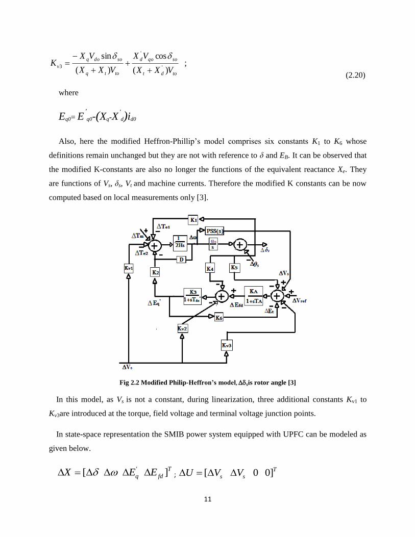
Also, here the modified Heffron-Phillip‘s model comprises six constants K1 to K6 whose

definitions remain unchanged but they are not with reference to δ and EB. It can be observed that

the modified K-constants are also no longer the functions of the equivalent reactance Xe. They

are functions of Vs, δs, Vt and machine currents. Therefore the modified K constants can be now

computed based on local measurements only [3].

Fig 2.2 Modified Philip-Heffron’s model, sis rotor angle [3]

In this model, as Vs is not a constant, during linearization, three additional constants Kv1 to

Kv3are introduced at the torque, field voltage and terminal voltage junction points.

In state-space representation the SMIB power system equipped with UPFC can be modeled as

given below.

T

fdq EEX ] [ ' ; T

ss VVU ]0 0 [

12

and UBXAX

(2.21)

where as

1

0

1

0

0

0 0 0

65

''

3

'

4

21

0

AA

A

A

A

dododo

TT

KK

T

KK

TT

K

T

K

M

K

M

D

M

K

A

;

0 0

0 0 0

0 0 0

0 0 0 0

3

'

2

1

A

vA

A

A

do

v

v

T

KK

T

K

T

K

M

K

B

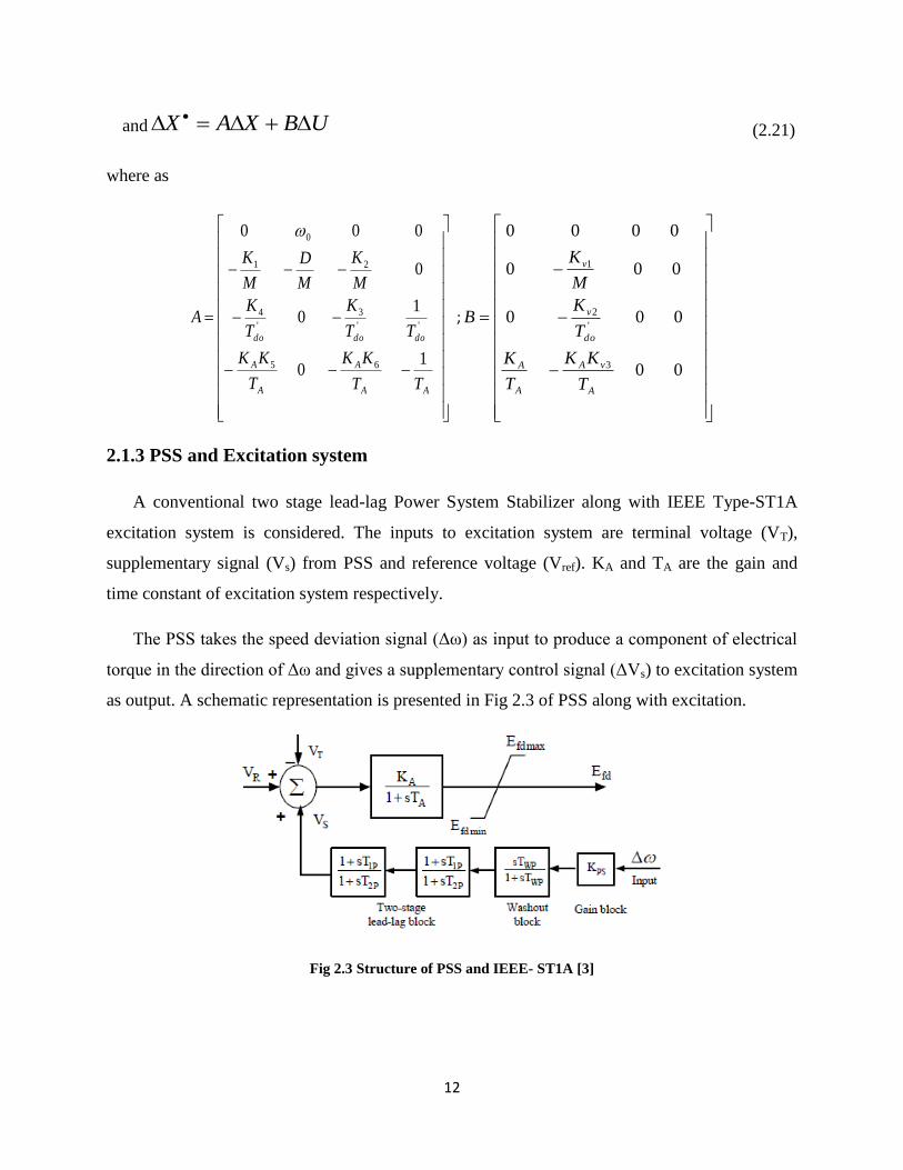
2.1.3 PSS and Excitation system

A conventional two stage lead-lag Power System Stabilizer along with IEEE Type-ST1A

excitation system is considered. The inputs to excitation system are terminal voltage (VT),

supplementary signal (Vs) from PSS and reference voltage (Vref). KA and TA are the gain and

time constant of excitation system respectively.

The PSS takes the speed deviation signal (Δω) as input to produce a component of electrical

torque in the direction of Δω and gives a supplementary control signal (ΔVs) to excitation system

as output. A schematic representation is presented in Fig 2.3 of PSS along with excitation.

Fig 2.3 Structure of PSS and IEEE- ST1A [3]

13

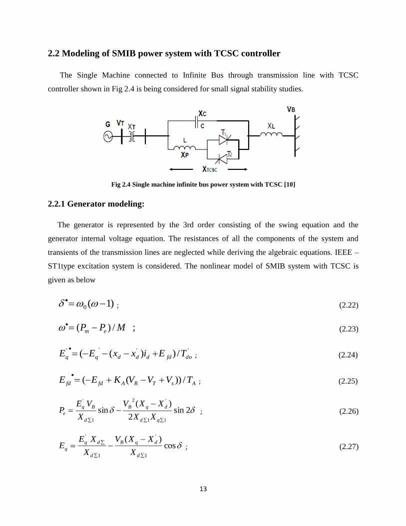
2.2 Modeling of SMIB power system with TCSC controller

The Single Machine connected to Infinite Bus through transmission line with TCSC

controller shown in Fig 2.4 is being considered for small signal stability studies.

Fig 2.4 Single machine infinite bus power system with TCSC [10]

2.2.1 Generator modeling:

The generator is represented by the 3rd order consisting of the swing equation and the

generator internal voltage equation. The resistances of all the components of the system and

transients of the transmission lines are neglected while deriving the algebraic equations. IEEE –

ST1type excitation system is considered. The nonlinear model of SMIB system with TCSC is

given as below

)1(0 ; (2.22)

; /)( MPP em (2.23)

'''' /))(( dofddddqq TEixxEE

; (2.24)

AsTRAfdfd TVVVKEE /))((

; (2.25)

2 sin 2

)(sin

11

'2

1

'

qd

dqB

d

Bq

eXX

XXV

X

VEP ; (2.26)

cos )(

1

'

1

'

d

dqB

d

dq

qX

XXV

X

XEE ; (2.27)

14

sin

1

q

Bq

TdX

VXV (2.28)

cos

1

'

1

'

d

dB

d

qEff

TdX

XV

X

EXV ; (2.29)

)(22

TqTdT VVV ; (2.30)

where

; )(TCSCCFLTEff XXXXX

; 1 Effqq XXX

; '

1 Effdd XXX

; Effdd XXX

The synchronous machine is described by 3rd

order model and the Philip-Heffron‘s model of

Single Machine Infinite Bus with TCSC controller is obtained by linearizing system equations

around an operating condition of Power system.

0 (2.31)

MDKEKK pq /]['

21

(2.32)

''

34

' /][ dofdqqq TEKEKKE

(2.33)

AfdvqAfd TEKEKKKE /])([ '

65

(2.34)

/ ,'/ ,/

/ ,/ ,/

/ ,/ ,/

65

'

34

'

21

TvqTT

qqqqq

epqee

VKEVKVK

EKEEKEK

PKEPKPK

(2.35)

15

The linearized Philip-Heffron‘s model of single machine infinite machine bus system with

TCSC and PSS is as shown in fig 2.5.

Fig 2.5 Phillips-Heffron model of SMIB with TCSC and PSS [10]

In state-space representation the SMIB power system equipped with UPFC can be modeled as

given below.

T

fdq EEX ] [ ' ; T

TCSCs XVU ]0 0 [

and UBXAX

(2.35)

where as

1

0

1

0

0

0 0 0

65

''

3

'

4

21

0

AA

A

A

A

dododo

TT

KK

T

KK

TT

K

T

K

M

K

M

D

M

K

A

;

0 0

0 0 0

0 0 0

0 0 0 0

3

'

2

1

A

vA

A

A

do

v

v

T

KK

T

K

T

K

M

K

B

16

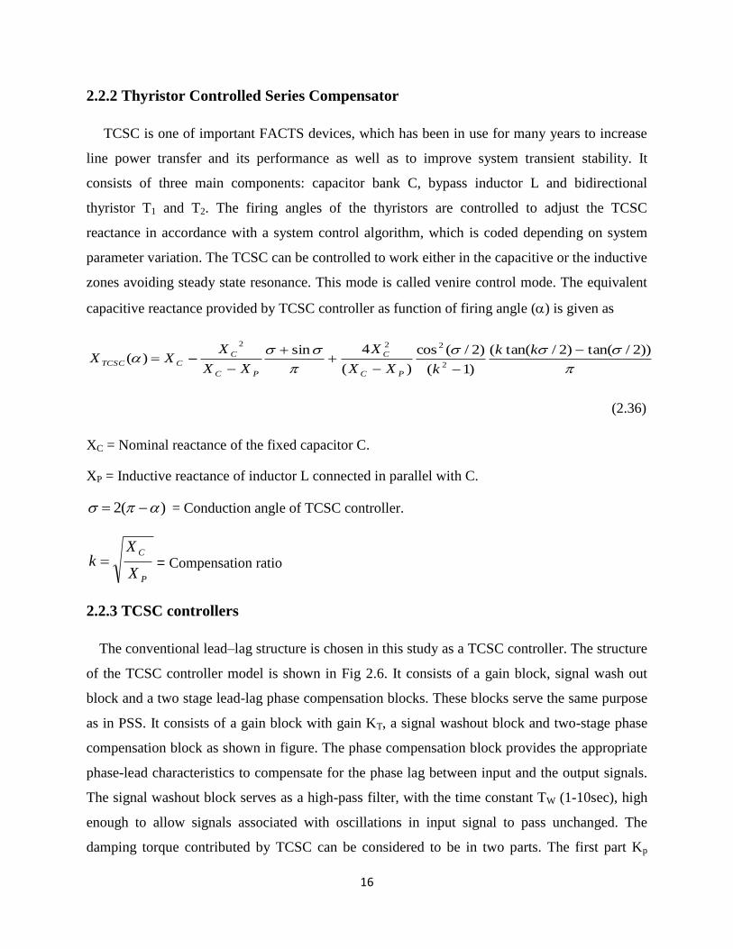
2.2.2 Thyristor Controlled Series Compensator

TCSC is one of important FACTS devices, which has been in use for many years to increase

line power transfer and its performance as well as to improve system transient stability. It

consists of three main components: capacitor bank C, bypass inductor L and bidirectional

thyristor T1 and T2. The firing angles of the thyristors are controlled to adjust the TCSC

reactance in accordance with a system control algorithm, which is coded depending on system

parameter variation. The TCSC can be controlled to work either in the capacitive or the inductive

zones avoiding steady state resonance. This mode is called venire control mode. The equivalent

capacitive reactance provided by TCSC controller as function of firing angle () is given as

))2/tan()2/tan((

)1(

)2/(cos

)(

4sin)(

2

222

kk

kXX

X

XX

XXX

PC

C

PC

C

CTCSC

(2.36)

XC = Nominal reactance of the fixed capacitor C.

XP = Inductive reactance of inductor L connected in parallel with C.

)(2 = Conduction angle of TCSC controller.

P

C

X

Xk = Compensation ratio

2.2.3 TCSC controllers

The conventional lead–lag structure is chosen in this study as a TCSC controller. The structure

of the TCSC controller model is shown in Fig 2.6. It consists of a gain block, signal wash out

block and a two stage lead-lag phase compensation blocks. These blocks serve the same purpose

as in PSS. It consists of a gain block with gain KT, a signal washout block and two-stage phase

compensation block as shown in figure. The phase compensation block provides the appropriate

phase-lead characteristics to compensate for the phase lag between input and the output signals.

The signal washout block serves as a high-pass filter, with the time constant TW (1-10sec), high

enough to allow signals associated with oscillations in input signal to pass unchanged. The

damping torque contributed by TCSC can be considered to be in two parts. The first part Kp

17

referred as direct damping torque and is directly applied to electro mechanical oscillation loop of

the generator. The second part comprises of both Kq and Kv referred as indirect damping torque,

applied through the field channel of generator. The damping torque contributed by TCSC

controller to the electromechanical oscillation loop of the generator is

DTP0DD KKKTT (2.37)

Fig 2.6 Structure of TCSC controller [10]

2.2.4 PSS and Excitation system

The conventional two-stage lead-lag Power System Stabilizer is considered in this study. IEEE

Type-ST1A Excitation system is considered. The inputs to excitation system are terminal voltage

(VT), supplementary signal (Vs) from PSS and reference voltage (Vref). KA and TA are the gain

and time constant of excitation system respectively.

Fig 2.7 Structure of PSS and IEEE Type-ST1A Excitation system [10]

The PSS takes the speed deviation signal (Δω) as input to produce a component of electrical

torque in the direction of Δω and gives a supplementary control signal (ΔVs) to excitation system

as output. It consists of a wash out block to reduce over response of damping during severe

18

events and acts as high pass filter, with time constant (Tw) high enough to allow signals

associated with oscillations in input signal to pass unchanged. The lead-lag compensation blocks

are responsible to produce a component of electrical torque in the direction of speed deviation

(Δω). The gain (Kp) determines the damping level.

2.3 Modeling of SMIB power system with UPFC controller

A SMIB power system model equipped with UPFC shown in Fig. 2.8 is used to obtain

linearized modified Philip-Heffron‘s model with UPFC.

Fig 2.8 Single machine infinite bus power system with UPFC [11]

The dynamic modeling of components in the power system like synchronous generator,

excitation system, AVR, UPFC etc. is needed for small signal stability studies.

2.3.1 Unified Power Flow Controller

The UPFC consists of a shunt connected excitation transformer (ET), series connected

boosting transformer (BT), two three-phase Gate Turn Off (GTO) based voltage source

converters (VSCs) and a common DC link capacitors. The four input control signals to the UPFC

are modulation index of shunt converter (mE), phase angle of the shunt-converter voltage (δE),

modulation index of series converter (mB) and phase angle of injected voltage (δB).

Two voltage converters VSC-E and VSC-B are operated from a common DC link provided

by a DC storage capacitor. The primary function of shunt converter is to supply the real power

demand to the series converter. It also regulates the terminal voltage of the interconnected bus by

controlling the reactive power supply to that bus. The series converter is controlled to inject a

19

voltage VBt in series with the line and its magnitude can be varied from 0 to VBt,max and its phase

angle can be varied independently from 00 to 360

0 see Fig 2.9 (a). A DC voltage regulator is

provided to maintain real power balance between two voltage converters. DC voltage is

regulated through modulating the phase angle of shunt converter voltage (δE) [11]. Equation for

real power balance between series and shunt converters is given as

Re 0 ) (

BBtEEt iViV

(2.38)

Fig 2.9 Phasor diagram showing the modulation of real power flow through bus voltage magnitude and

phase regulation [11].

A UPFC can perform voltage regulation via the addition of an in-phase voltage VBt=V0, see

Fig 2.9(b). Voltage regulation and series reactance compensation is carried out through the

addition of VBt=V0+Vp, where V0 is in phase with the bus voltage Vi and Vp is out-of phase with

the line current by 90°, see Fig 2.9 (c). Fig 2.9 (d) illustrates the process of phase-shifting. In

here, the voltage phasor to be added VBt=V0+Vφ, where V0 is in phase with the bus voltage and Vφ

shifts the resulting voltage phasorVBt+V0 by an angle φ [11].

2.3.2 Nonlinear dynamic model

A non-linear dynamic model of the system is derived by disregarding the resistances of all

components of the system (generator, transformers, transmission lines and converters) and the

20

transients of the transmission lines and transformers of the UPFC [11, 19, 21]. The nonlinear

dynamic model of the system installed with UPFC is described by the following set of equations.

)1( o (2.39)

/))1(( MDPP em (2.40)

/))(( ''''

doqdddfdq TEixxEE

(2.41)

/))(( AfdpssrefAfd TEuvVKE

(2.42)

)sincos(4

3 )sincos(

4

3BBqBBd

dc

BEEqEEd

dc

Edc ii

C

mii

C

mv

(2.43)

)]([)(''

BdEddqBqEqqqd iixEjiixjvvv

(2.44)

qqdde ivivP

(2.45)

BdEdd iii

(2.46)

2

cos dcEEEqEEtd

vmixv

(2.47)

2

sin dcEE

EdEEtq

vmixv

(2.48)

BqEqq iii

(2.49)

2

cos dcBB

BqBBtd

vmixv

(2.50)

2

sin dcBB

BdBBtq

vmixv

(2.51)

cossin bbBqBVBdBVBtqBtdEtqEtd jvvixijxjvvjvv

(2.52)

21

)2

sin cos(

2

sin' dcBB

b

d

dE

d

BddcEE

q

d

BBEd

vmv

x

x

x

xvmE

x

xi

(2.53)

)2

sincos(

2

sin' dcBB

b

d

dt

d

dEdcEE

q

d

E

Bd

vmv

x

x

x

xvmE

x

xi

(2.54)

)2

cossin(

2

cosdcBB

b

q

qE

q

BqdcEE

Eq

vmv

x

x

x

xvmi

(2.55)

)2

cossin(

2

cosdcBB

b

q

qt

q

qEdcEE

Bq

vmv

x

x

x

xvmi

(2.56)

where

)())(( tEqEBVBEtEqq xxxxxxxxx

)())((''

tEdEBVBEtEdd xxxxxxxxx

tEqBvBBq xxxxx ; tEdBvBBd xxxxx '

;

tEEqqt xxxx ; tEEddt xxxx '; tEddE xxx '

tEdqE xxx ; BvBBB xxx

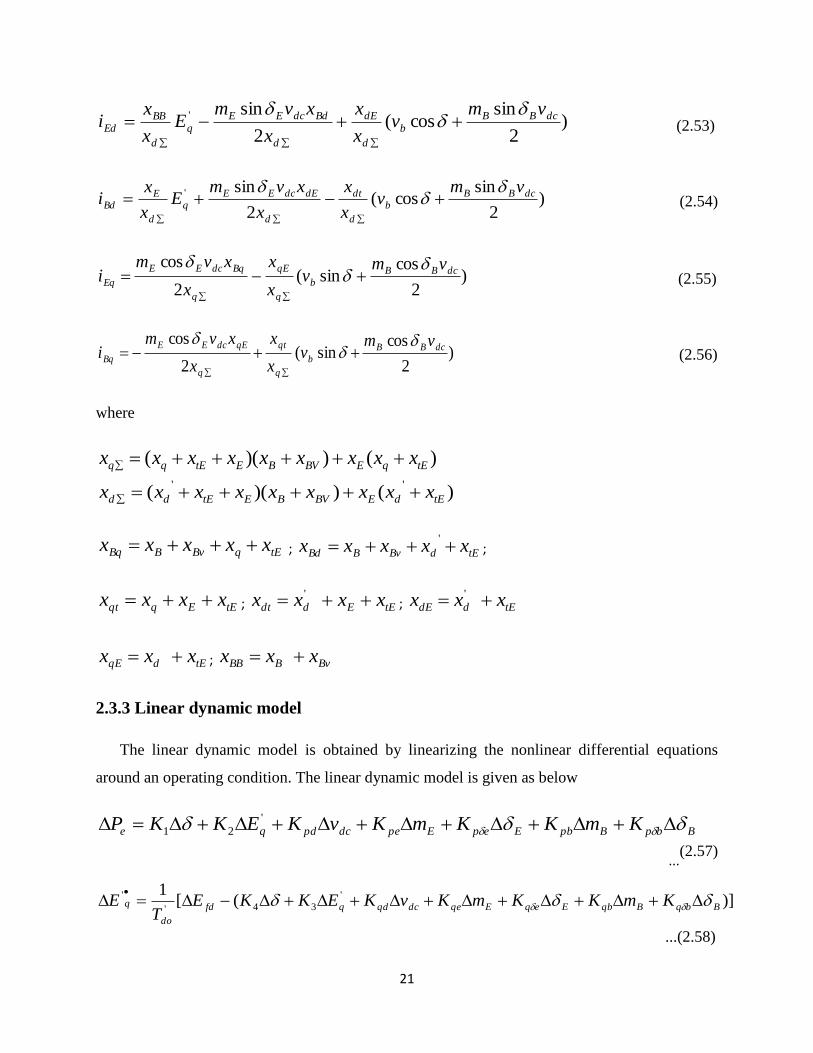
2.3.3 Linear dynamic model

The linear dynamic model is obtained by linearizing the nonlinear differential equations

around an operating condition. The linear dynamic model is given as below

'

21 BbpBpbEepEpedcpdqe KmKKmKvKEKKP

...(2.57)

)] ([1 '

34'

'

BbqBqbEeqEqedcqdqfd

do

q KmKKmKvKEKKET

E

...(2.58)

22

'

65 BbvBvbEevEvedcvdq KmKKmKvKEKKv

...(2.59)

9

'

87 BbcBcbEecEcedcqdc KmKKmKvKEKKv

...(2.60)

In state-space representation the SMIB power system equipped with UPFC can be modeled

as given below.

T

dcfdq vEEX ] [ ' ; T

bbEEpss mmuU ] [

and UBXAX

(2.61)

where as

987

55

'''

3

'

4

21

0

0 0

1

0

1

0

0

0 0 0 0

KKK

T

KK

TT

KK

T

KK

T

K

TT

K

T

K

M

K

M

K

M

D

M

K

A

A

vdA

AA

A

A

A

do

qd

dododo

pd

;

bccbecce

A

bvA

A

vbA

A

evA

A

veA

A

A

do

bq

do

qb

do

eq

do

qe

bppbeppe

KKKK

T

KK

T

KK

T

KK

T

KK

T

K

T

K

T

K

T

K

T

K

M

K

M

K

M

K

M

K

B

0

0

0

0 0 0 0 0

''''

23

Fig 2.10 Linear Philip-Heffron model of SMIB power system with UPFC [11]

2.3.4 Excitation system and PSS

The conventional two stage lead-lag power system with IEEE-ST1 type excitation system

is considered. For the excitation system inputs are terminal voltage (VT), supplementary signal

Fig 2.11 IEEE type - ST1 excitation system with PSS [11]

(Vs) from PSS and reference voltage (Vref). KA and TA are the gain and time constant of

excitation system respectively. The PSS takes the speed deviation signal (Δω) as input to

produce a component of electrical torque in the direction of Δω and gives a supplementary

24

control signal (ΔVs) to excitation system as output. A schematic representation is presented in

Fig. 2.11 of PSS along with excitation.

2.3.5 UPFC damping controllers

The lead-lag damping controllers are designed to produce a component of electrical torque in

the direction of speed deviation to produce sufficient positive damping in order to provide

damping on small frequency power system oscillations. The four control parameters (mB, mE, δB,

δE) are modulated to produce sufficient damping. The parameter mB controls the magnitude of

series voltage injected, there by controls the reactive power compensation. By varying the

parameter δB the real power flow can be controlled. The parameter mE can be modulated to

control the voltage at the bus where UPFC is installed. The damping controllers for mB, mE, δB

are as shown below, where ‗u‘ may be any of the mB, mE, δB.

Fig 2.12 Structure of Lead-lag UPFC controller (mB, mE, δB) [11]

The parameter δE can be modulated to regulate the DC voltage at DC link. So, the δE

damping controller as shown below is provided with a PI controller, which functions as DC

voltage regulator.

Fig 2.13 Structure of δELead-lag controller with DC voltage regulator [11]

25

CHAPTER 3

Problem formulation

3.1 Modified Philip-Heffron’s model

3.1.1 Structure of PSS

The conventional lead–lag structure is chosen in this study. It consists of a gain block with

gain KPSS, a signal washout block and two-stage phase compensation block as shown in Fig 2.14.

The phase compensation block provides the appropriate phase-lead characteristics to compensate

for the phase lag between input and the output signals. The signal washout block serves as a

high-pass filter, with the time constant TW (1-10 sec), high enough to allow signals associated

with oscillations in input signal to pass unchanged. Transfer function of PSS is given by

1

1

1

1

1 4

3

2

1

sT

sT

sT

sT

sT

sTKV

W

WPSSs

(3.1)

In this design TW is usually pre-specified. The gains KPSS and T1, T2, T3, T4 are to be

determined. The input signal of the proposed PSS is the speed deviation (Δω) and the output is

supplementary signal (Vs).

3.1.2) PID-PSS controller

Transfer function of PID-PSS is given by

)(1

1

1

1

1 4

3

2

1 sGsT

sT

sT

sT

sT

sTKV c

W

WPSSs

(3.2)

where

)()( sKs

KKsG d

ipc

26

Fig 2.14 Structure of Lead-lag PSS with PID controller

The proportional gain Kp provides a control action proportional to the error and reduces the

rise time. The integral gain Ki reduces the steady state error by performing an integral control

action and eliminates the steady state error. The derivative term Kd improves the stability of the

system and reduces the overshoot by improving the transient response. Hence, ABC is used to

determine optimal Kp, Ki, Kd values.

3.1.3 Time Domain based Objective function

The performance of the system considered depends on the controller parameters, which in

turn depends on the objective function to be minimized. The design of PSS is done based on

minimizing the objective function considered in order to reduce the power system oscillations

after a disturbance in loading condition so as to improve the stability of power system. In this

paper the objective function is formulated in such a way that rotor speed deviation is minimized

and is mathematically formulated as follows

d )],([0

2

t

tXttJ

(3.3)

In the Eqn (3.3), Xt, denotes the rotor speed deviation for a set of controller parameters

X. Here X represents the parameters to be optimized. The optimization is carried in two phases,

initially the 5 parameters corresponding to PSS controller are been tuned and in second phase by

fixing the obtained parameters of PSS controller, the PID parameters Kp, Ki and Kd are tuned to

obtain optimum system response.

27

3.2 Single Machine Infinite Bus System with TCSC controller

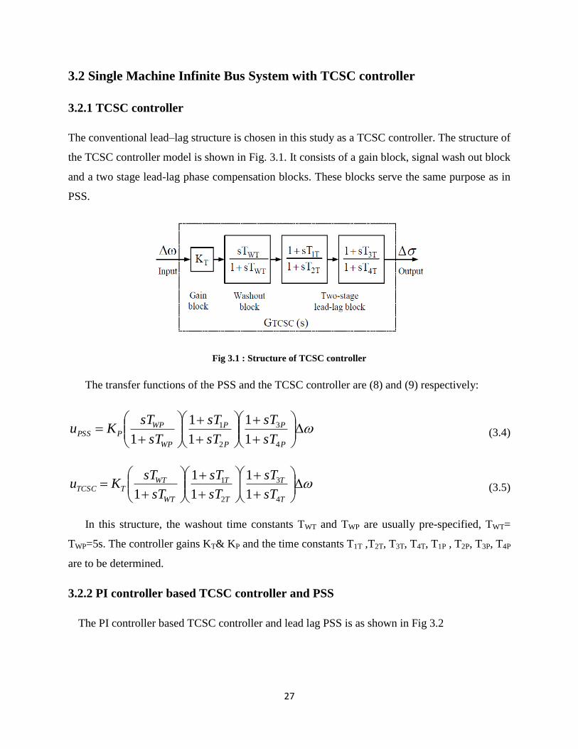
3.2.1 TCSC controller

The conventional lead–lag structure is chosen in this study as a TCSC controller. The structure of

the TCSC controller model is shown in Fig. 3.1. It consists of a gain block, signal wash out block

and a two stage lead-lag phase compensation blocks. These blocks serve the same purpose as in

PSS.

Fig 3.1 : Structure of TCSC controller

The transfer functions of the PSS and the TCSC controller are (8) and (9) respectively:

P

P

P

P

WP

WPPPSS

sT

sT

sT

sT

sT

sTKu

4

3

2

1

1

1

1

1

1 (3.4)

T

T

T

T

WT

WTTTCSC

sT

sT

sT

sT

sT

sTKu

4

3

2

1

1

1

1

1

1 (3.5)

In this structure, the washout time constants TWT and TWP are usually pre-specified, TWT=

TWP=5s. The controller gains KT& KP and the time constants T1T ,T2T, T3T, T4T, T1P , T2P, T3P, T4P

are to be determined.

3.2.2 PI controller based TCSC controller and PSS

The PI controller based TCSC controller and lead lag PSS is as shown in Fig 3.2

28

Fig 3.2 : Structure of TCSC controller and PSS with PI controller

The proportional gain Kp provides a control action proportional to the error and reduces the

rise time. The integral gain Ki reduces the steady state error by performing an integral control

action and eliminates the steady state error. Transfer functions of PSS and TCSC controllers with

PI controllers are

)(

1

1

1

1

1 4

3

2

1 sGsT

sT

sT

sT

sT

sTKu

P

P

P

P

WP

WPPPSS (3.6)

)(

1

1

1

1

1 4

3

2

1 sGsT

sT

sT

sT

sT

sTKu

T

T

T

T

WT

WTTTCSC (3.7)

wheres

KKsG i

p )(

The input signal of the TCSC stabilizer is the speed deviation Δω and the output is change in

conduction angle. During steady state conditions XEff= XT+XLXTCSC() and.During

dynamic conditions theseries compensation is modulated for damping system oscillations. The

effective reactance in dynamic conditions is: XEff= XT+XLXTCSC(), where&,

andbeing initial value of firing & conduction angle respectively.

3.2.3 Time Domain based Objective function

The design of coordinated controller is done based on minimizing the objective function

considered such that power system oscillations after a disturbance or loading condition so as to

improve the stability. In this approach the objective function is formulated in such way rotor

speed deviation (is minimized and mathematically formulated as follows

29

1

0

2),(

t

dtXttJ

(3.8)

In the above equations, t, X) denotes the rotor speed deviation for a set of controller

parameters X. Here X represents the parameters to be optimized. The optimization is carried in

two phases, initially the 10 parameters corresponding to both TCSC and PSS controller are been

tuned coordinately and in second phase by fixing the obtained parameters of TCSC and PSS

controllers, the PI parameters Kp and Ki of both TCSC and PSS are tuned coordinately to obtain

optimum system response.

3.2 Single Machine Infinite Bus System with UPFC controller

3.3.1 Structure of UPFC damping controller

The conventional lead–lag structure is chosen for UPFC damping controllers in this study. It

consists of a gain block with gain K, a signal washout block and two-stage phase compensation

block as shown in Fig. 2.1.2 and 2.1.3. The phase compensation block provides the appropriate

phase-lead characteristics to compensate for the phase lag between input and the output signals.

The signal washout block serves as a high-pass filter, with the time constant TW(5 sec), high

enough to allow signals associated with oscillations in input signal to pass unchanged.

In this design TW is usually pre-specified. The gains K and T1, T2, T3, T4 are to be determined.

The input signal of the proposed damping controllers is the speed deviation (Δω) and the output

is supplementary signal is u (mB, mE, δB, δE).

3.3.2 PI controller based UPFC damping controllers:

The PI controller based lead lag damping controllers for mB, δEandδBis as shown below,

where ‗u‘ may be any of the mB, δE or δB. The proportional gain Kp provides a control action

proportional to the error and reduces the rise time. The integral gain Ki reduces the steady state

error by performing an integral control action and eliminates the steady state error.

30

Fig 3.3 Structure of PI controller based mB, δE or δBdamping controllers

3.3.3 Time Domain based Objective Function

The performance of the system considered depends on the controller parameters, which in

turn depends on the objective function to be minimized. The design of damping is done based on

minimizing the objective function considered in order to reduce the power system oscillations

after a disturbance in loading condition so as to improve the stability of power system. In this

paper the objective function is formulated in such a way that rotor speed deviation is minimized

and is mathematically formulated as follows

d )],([0

2

t

tXttJ

(3.9)

In the Eqn. (3.9), t, X) denotes the rotor speed deviation for a set of controller parameters

X. Here X represents the parameters to be optimized. The optimization is carried in three phases,

initially the 5 parameters corresponding to each of the two individual controllers considered in

each case are been tuned and in second phase coordinated tuning of total 10 parameters

corresponding to both controllers considered is carried out. In the case of nominal and heavy

loading conditions SMIB system with mE, δB controllers have shown relatively lower stability

than that of system without UPFC (only PSS). So, in the case of nominal and heavy loading

conditions only mB, δE controllers are considered for tuning. In the case of light loading condition

SMIB system with mE, δE controllers have shown relatively lesser stability than that of system

without UPFC (only PSS). So, in the case of nominal and heavy loading conditions only mB, δB

controllers are considered for tuning.

31

In third phase PI controllers of selected UPFC damping controllers for particular loading

condition are tuned to achieve optimum system performance. In this phase totally 4 parameters

(Kp and Ki of either mE and δB controllers for nominal and heavy loaded conditions or mB and δE

controllers for light loaded condition) has been tuned using ABC algorithm.

32

CHAPTER 4

Artificial Bee Colony Algorithm

4.1 Biological Motivation

Honey bees live in extremely populous colonies and maintain a unique elaborated social

organization. The exchange of information among bees leads to the formation of tuned collective

knowledge. Virtually the bee colony consists of a single ―queen bee‖, a few hundred drones

(males), and tens of thousands of workers (non-reproductive females). Female (worker) bees,

probably at their early stages of age, begin foraging for food making trip after trip.

The minimal model of forage selection that leads to the emergence of collective intelligence

in honey bee swarms consists of the following essential components:

i) Food Sources: The value of a food source depends on several factors such as its proximity to

the nest, its richness or concentration of energy and ease of extracting this energy. In other

words, the ―profitability‖ of foods source can be represented in single quantity.

ii) Employed Foragers: They are associated with a particular food source, which are being

exploited. They carry with them information about this particular source such as its distance

(and also direction) from nest and share this information with certain probability.

iii) Unemployed Foragers: They are continually looking for a food source to exploit. There are

two types of unemployed foragers: scouts searching the environment and surrounding the nest

for new food sources and onlookers waiting in the nest and searching a food source through

the information shared by employed foragers.

The exchange of information among bees plays a key role in the formation of collective

knowledge. Communication among bees related to the quality of food occurs in dancing area of

hive. This dance is called round dance or waggle dance (based on the distance of food source

from the hive. Employed foragers share their information with a probability proportional to the

food source and sharing of this information through waggle dancing is longer in duration. Hence

33

the recruitment is directly proportional to the profitability of the food source.

4.2 The Algorithm

Artificial Bee Colony (ABC) is an optimization algorithm inspired by the foraging behavior of

honey bees. It was proposed and investigated by Karaboga et al. [24, 25, 32] for derivative-free

optimization of nonlinear, non-convex and multi-modal objective functions. The ABC algorithm

classifies the foraging artificial bees into three groups namely employed bees, onlooker bees,and

scout bees. First half of the colony consists of employed bees while the second half consists of

onlooker bees. A bee that is currently searching for food or exploiting a food source is called an

employed bee and a bee waiting in the hive for making decision to choose a food source is

termed as an onlooker. For every food source, there is only one employed bee and the employed

bee of abandoned food source becomes scout. In ABC, each solution to the problem is

considered as a food source and is represented by a D-dimensional real-valued vector, whereas

the fitness of the solution corresponds to the nectar amount of the associated food resource. Like

other swarm based algorithms, ABC also progresses through iterations.

It starts with population of randomly distribute solutions or food sources. The following steps

are repeated until a termination criterion is met.

i) At the initial stages of foraging, calculate the nectar amounts by sending the employed bees

on to the food sources.

ii) After sharing the information from employed bees select the food sources by the onlookers

and determine the nectar amount of food sources.

iii) Determine the scout bees and send them randomly to find out new food sources, if the bee

source is exhausted.

The main components of ABC are briefly explained below.

i) Initialization of Parameters:

The basic parameters of ABC algorithm are number of food sources (FS) which is equal to

number of employed bees (ne) or onlooker bees (no), the numbers of trails after which food

34

sources are assumed to be abandoned (limit) is set with help of parameter limit and the last

parameter is termination criterion. In ABC algorithm the number of employed bees is set equal to

number of food sources in the population i.e., for every food source there is one employed bee.

ii) Initialization of Individuals (bees):

The algorithm starts by initializing all employed bees with randomly generated food sources.

In general the position of i-th food source that corresponds to a solution in the search space is

represented as ,1 ,2 ,[ , ,..., ]i i i i DX x x x and is initially generated by the following equation:

, , [0,1].( ),i j j i j j jx lb rand ub lb

(4.1)

where 1,2,...., ,i FS 1,2,...., ,j D and , [0,1]i jrand is a uniformly distributed random number in [0,

1] and it is instantiated anew for each j-th component of the i-th food source. ubj and lbj denote

the upper and lower bounds for j-th dimension respectively. Now food sources are assigned

randomly to bees and hereafter new food sources are exploited by employed as well as onlooker

bees and explored by scout bees in repeated cycles.

iii) Exploitation of new food sources via employed bee:

A new food source is generated by each employed bee in the neighborhood of its present

position depending on local information. The new food source is exploited by perturbing any one

randomly selected dimension of the current food source in the following way:

, , , , ,.( ),i j i j i j i j k jv x x x (4.2)

where iV is the new food source in neighborhood of ,iX FSk ,....,3,2,1 such that ik and

Dj ,...,3,2,1 are randomly chosen indices. ,i j is an uniformly distributed random number in the

range [-1,1]. ,i j controls the amplitude of the perturbation term. Nectar amount or fitness of iV

for a minimization problem is defined as:

1/ (1 ( )), if ( ) 0,

1 ( ( )), if ( ) 0,

i i

i

i i

f V f Vfit

abs f V f V

(4.3)

35

where f is the function to be minimized. Once the new solution is obtained, a greedy selection

mechanism is employed between the old and the new candidate solutions i.e., iX and iV . Then

the better one is selected depending on the fitness values. If the source at iV is better than that at

iX in terms of profitability, the employed bee memorizes the new position and discards the old

one. If iX cannot be improved, its counter holding the number of trails is incremented by 1,

otherwise, the counter is reset to 0.

iv) Determining probability values for selection:

When all employed bees complete their foraging, they get ready to perform different dances

to share the information about nectar amounts and the position of their sources with the onlooker

bees in the dance area. An onlooker bee carefully observes the nectar information from all

employed bees and selects a food source site with a probability related to its nectar amount and

this probabilistic selection is dependent on fitness values of the solutions in population. In ABC,

roulette wheel fitness-based selection scheme is incorporated. Selection probability of the i-th

food source is given by:

1

,ii FS

k

k

fitp

fit

(4.4)

where ifit is the fitness value of the i-th food source iX .

(v)Exploitation of food sources by Onlooker bees based on information shared by employed

bees:

In ABC algorithm, for each food source a random real number in range [0, 1] is generated. If

the probability value in Eqn. (4) associated with that source is greater than the produced random

number then the onlooker bee produces modification on its food source position by making use

of Eqn. (2). After the source is evaluated, greedy mechanism is applied and counters are either

incremented by 1 or reset to 0 based on the counters holding trails (a similar mechanism as that

of the employed bees).

36

vi) Exploration of new food sources by Scout bees:

In a cycle of this cyclic process, after all employed and onlooker bees complete their

searches; the algorithm is made to check if there is any exhausted food source that needs to be

abandoned, the counters which have been updated during each search are been used. If the value

of a counter is greater than the limit then the source associated with this counter is abandoned.

Abandoned food source by a bee is replaced by a new food source discovered by the scout. This

is done by producing a site position randomly and replacing with abandoned one. This operation

is similar to that of initializing a new food sources to unemployed bee (discussed in earlier

section). Below we provide a simplified pseudo-code of the ABC algorithm.

Summary of Artificial Bee Colony Algorithm

1. Initialization

2. Move the Employed Bees onto their Food sources and evaluate their nectar amounts

3. Place the onlookers depending upon the nectar amounts obtained from employed

bees.

4. Send the scouts for exploiting new food sources

5. Memorize the best food sources obtained so far

6. If a termination criterion is not satisfied, go to step 2; otherwise stop the procedure

and display the best food source obtained so far.

Pseudo Code of ABC Algorithm

Step1. Initialize the population of solutions ,ijx FSi ,....2,1 , ,,....2,1 Dj 0itrail ; itrail is

the non-improvement number

Step2. Evaluate the population

Step3. Cycle=1

Step4. REPEAT

{------------Produce new food source population for employed bee-------------}

Step5. For i=1 to FS do

37

i. Produce a new food source iv for the employed bee of the food source ix by

using (4.3) evaluate its quality

ii. Apply a greedy selection process between iv and ix , then after select the better

one

iii. If solution ix doesn‘t improve 1 ii trailtrail , otherwise 0itrail ;

End For

Step6. Calculate the probability values iP by (1) for the solutions using fitness values.

{------------Produce new food source population for employed bee-------------}

t=0;

i=1;

Step7. REPEAT

IF iPrand then

i. Produce a new food source ijv for the employed bee of the food source ix by

using (4.3) and evaluate the quality.

ii. Apply a greedy selection process between iv and ix , then after select the better

one

iii. If solution ix doesn‘t improve 1 ii trailtrail , otherwise 0itrail ;

iv. t=t+1

End If

UNTIL (t=FS)

{---------Scout phase--------}

Step8. If max(trail) > limit then

i. Replace 1x with a new randomly produce solution by using following equation

)(*)1,0( minmaxmin

jjjij xxrandxx

38

End If

ii. Memorize the best solution achieved so far

Cycle=Cycle+1;

UNTIL (Cycle=Maximum Cycle number)

39

CHAPTER 5

EXPERIMENTAL SECTION

5.1) System parameters of SMIB system considered for Modified Philip-

Heffron model analysis

For the small signal stability analysis of SMIB the design of the system and system data is

taken from [3].

1. System data: All data are in p.u unless specified otherwise

2. Generator: H=5 s, D=0, Xd=1.6, Xq=1.55, Xd‘ =0.32, Td0=6, machine

3. Exciter: (IEEE type ST1) KA=200, TA=0.05s, Efd max=6 p.u & Efd min= -6 p.u

4. Transformer: XT=0.1

5. CPSS data: T1=T3=0.078, T2=T4=0.026, KPSS=16, TW=2, PSS output limits 0.05

6. Mod HP-CPSS: T1= T3=0.0952, T2= T4=0.0217, KPSS=13, TW=2, PSS output limits 0.05

As the optimization is carried out within bounds the following ranges are considered for the

parameters to be tuned. The parameters being considered for tuning were KPSS, T1, T2, T3, T4 and

Kp, Ki and Kd. Maximum and minimum parameters considered are as follows.10<Kpss<80;

0.05<T1,T3<0.6; 0.02<T2, T4<0.4; 0<KP,KI<50; 0<Kd<10.

5.2 System parameters of SMIB with TCSC controller

For the small signal stability analysis of single machine infinite bus the design of the system

and system data is taken from [10].


2. Generator: H=4.0s, D=0, Xd=1.0, Xq=0.6, Xd’ =0.3, Td0

‘=5.044, f=50, Ra=0, VT=1.05.

3. Exciter: (IEEE type ST1) KA=200, TA=0.04s.

4. Transmission line and Transformer: =0.0+j0.8 (XL=j0.7, XT=0.1)

40

5. TCSC Controller: XTCSC 0=0.245, ,04.156 0

0 XC=0.21, XP=0.0525

As the optimization is to be carried out in a bounded search we had used the following ranges

for different parameters in our design. The parameters being considered for tuning were KT, KP,

T1T, T2T, T3T, T4T, T1P, T2P, T3P, T4Pand PI controller parameters (Kp, Ki) of both TCSC and PSS

controllers.(the parameters with subscript T indicates they belong to TCSC controller and that of

P indicates they belong to PSS Control. The ranges over which these parameters tuned as per

standards are 30< KP, KT<80 & 0.1 <T1T, T3T, T1P, T3P < 0.6 & 0.02 < T2T, T4T, T2P, T4P< 0.4 & 0

<Kp< 50, 0 < Ki< 10.

5.3 System parameters of SMIB with UPFC controller

For the small signal stability analysis of SMIB the design of the system and system data is

taken from [11].


2. Generator: H=4.0 s, D=0, Xd=1.0, Xq=0.8, Xd’ =0.3, Td0‘=5.044, f=60p.u v=1.05

3. Exciter: (IEEE type ST1) KA=50, TA=0.05s, Efd max=7.3 p.u & Efd min= -7.3 p.u

4. Transformer and transmission line: = XtE=0.1 and XBV=0.6

5. PSS data: TW=5;Ti_min=0.01;Ti_max=5.0 where i=1, 2, 3& 4

PSS output limits = 0.2

6. UPFC data: XE=XB=0.1 and mB=0.0789,δB= -78.21740, mE=0.4013,δE= -85.3478

0mB and mE

output limits = 0 to 1 Ks=1 and Ts=0.05

7. DC link: VDC=2 p.u, CDC=3 p.u

As the optimization is carried out within bounds the following ranges are considered for the

parameters to be tuned. The parameters being considered for tuning were K, T1, T2, T3, T4.

Maximum and minimum parameters considered are as follows 0.01< T1, T2, T3, T4<5.0 and for

different controllers indicated with sub scripts 0<KmB<100 and -100<KmE, KδB, KδE<0 [1].

5.4 Parameters of ABC algorithm considered for tuning:

The objective function considered is a maximum of 10-Dimensional optimization function

hence we considered a maximum of 4000 Functional Evaluations as a termination criterion for

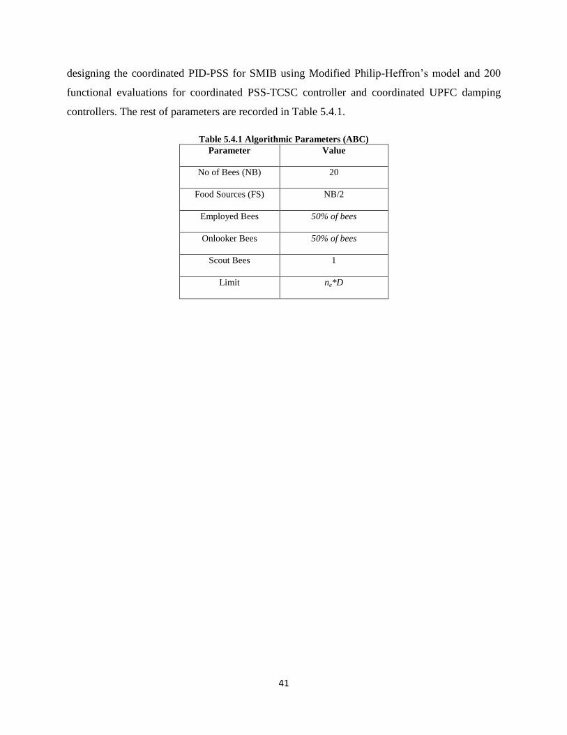
41

designing the coordinated PID-PSS for SMIB using Modified Philip-Heffron‘s model and 200

functional evaluations for coordinated PSS-TCSC controller and coordinated UPFC damping

controllers. The rest of parameters are recorded in Table 5.4.1.

Table 5.4.1 Algorithmic Parameters (ABC)

Parameter Value

No of Bees (NB) 20

Food Sources (FS) NB/2

Employed Bees 50% of bees

Onlooker Bees 50% of bees

Scout Bees 1

Limit ne*D

42

CHAPTER 6

Simulations and Results

6.1 Simulations for PID-PSS controller using Modified Philip-Heffron’s model

for SMIB system

The loading conditions considered for this study are summarized in the following table as

shown below.

Table 6.1.1: Loading conditions considered (p.u)

Nominal Loading or

Nominal system

Ps=1.0, Qs=0.2

Heavy Loading or strong

system

Ps=0.8,Qs=0.37

Light Loading or weak

system

Ps=1.0 ,Qs=0.5

The parametric values of Power system stabilizer obtained by tuning with ABC algorithm are

tabulated as follows

Table 6.1.2: Parametric Values Obtained for PSS Using ABC

Parameter Nominal

System

Strong

System

Weak

System

KPSS 40.7576 19.5975 19.8468

T1 0.1084 0.4227 0.1991

T2 0.0200 0.0200 0.0200

T3 0.6000 0.1818 0.2020

T4 0.3411 0.3792 0.4000

The parametric values of PID controller obtained by tuning with ABC algorithm are

tabulated as follows

43

Table 6.1.3: Parametric Values Obtained for PID Using ABC

Parameter Nominal

System

Strong

System

Weak

System

KP 26.0326 21.0599 9.9071

Ki 14.7003 9.5978 4.1251

Kd 0.8354 0.4256 0.3348

Table 6.1.4: Mean and Standard Deviation (std) without and with PID controller

Loading Condition

without PID controller

With PID controller

Nominal system 8.268e-04

(2.359e-06)

8.02e-04

(1.9525e-06)

Strong system 2.494e-03

(4.0518e-06)

2.3801e-03

(3.8243e-06)

Weak system 2.0196-03

(2.3082e-06)

1.9707e-03

(1.973e-06)

For a given 10% step change in input Tm, the responses obtained for nominal, strong and

weak systems are depicted in terms of speed deviation and rotor angle deviations. Fig 6.1 and 6.2

shows the rotor angle deviation and the speed deviation responses respectively for the heavy

loaded system.

44

Fig 6.1 Speed deviation for a step change of 10% in Vref for heavy loaded or strong system

Fig 6.2 Rotor angle deviation for a step change of 10% in Vref for strong system

0 1 2 3 4 5-5

-4

-3

-2

-1

0

1

2x 10

-3

time (sec)

Speed d

evia

tion (

p.u

)

Mod P-H model PSS

ABC tuned Mod P-H model PSS

ABC tuned Mod P-H model PID-PSS

0 1 2 3 4 5 6 7-0.6

-0.5

-0.4

-0.3

-0.2

-0.1

0

0.1

time (sec)

roto

r angle

devia

tion

Mod P-H model PSS


ABC tuned Mod P-H model PID-PSS

45

From Fig 6.1 and 6.2 the time domain indices recorded in Table 6.1.5 it is clear that proposed

PID controller based PSS tuned with ABC has produced less peak over shoot and low settling

time of speed deviation response.

Similarly Fig 6.3 and 6.4 show the speed deviation and rotor angle deviation responses for

lightly loaded system. The proposed PID based ABC tuned PSS controller has shown less

settling time and peak over shoot for speed deviation response. Also it has shown less settling

time for rotor angle deviation response.

Fig 6.3 Speed dev. for a step change of 10% in Vref for weak system

0 1 2 3 4 5-5

-4

-3

-2

-1

0

1

2

3x 10

-3

time(sec)

Speed d

evia

tion

Mod P-H model PSS

ABC tuned Mod P-H PSS

ABC tuned Mod P-H PID-PSS

46

Fig 6.4 Rotor angle dev. for a step change of 10% in Vref for weak system

Fig 6.5 Speed dev. for a step change of 10% in Vref for nominal

0 1 2 3 4 5-0.45

-0.4

-0.35

-0.3

-0.25

-0.2

-0.15

-0.1

-0.05

0

0.05

time(sec)

roto

r angle

devia

tion

Mod P-H PSS


ABC tuned Mod P-H PID-PSS

0 1 2 3 4 5-3.5

-3

-2.5

-2

-1.5

-1

-0.5

0

0.5

1x 10

-3

time(sec)

Speed d

evia

tion

Mod P-H model PSS


ABC tuned Mod P-H PID - PSS

47

Fig 6.5 and 6.6 depict the speed deviation and rotor angle deviations for the nominal loaded

system. PID based PSS controller tuned with ABC algorithm has shown relatively less settling

time and less peak over shoot value for rotor angle deviation response. For nominal loaded

system ABC tuned PSS has produced less settling time when compared to ABC tuned PID-PSS.

Fig. 6.6 Rotor angle dev. for a step change of 10% in Vref for nominal system

Finally Fig 6.7 and 6.8 show the convergence characteristics of ABC algorithm towards

optimum values without and with PID controller respectively. The parameters obtained via

optimal tuning are recorded in Table 6.1.2 and Table 6.1.3. From both the tables it is further

evident that objective function value is less for the PI controller case.

0 1 2 3 4 5-0.12

-0.1

-0.08

-0.06

-0.04

-0.02

0

0.02

time (sec)

roto

r angle

devia

tion

Mod P-H model PSS


ABC tuned Mod P-H model PID- PSS

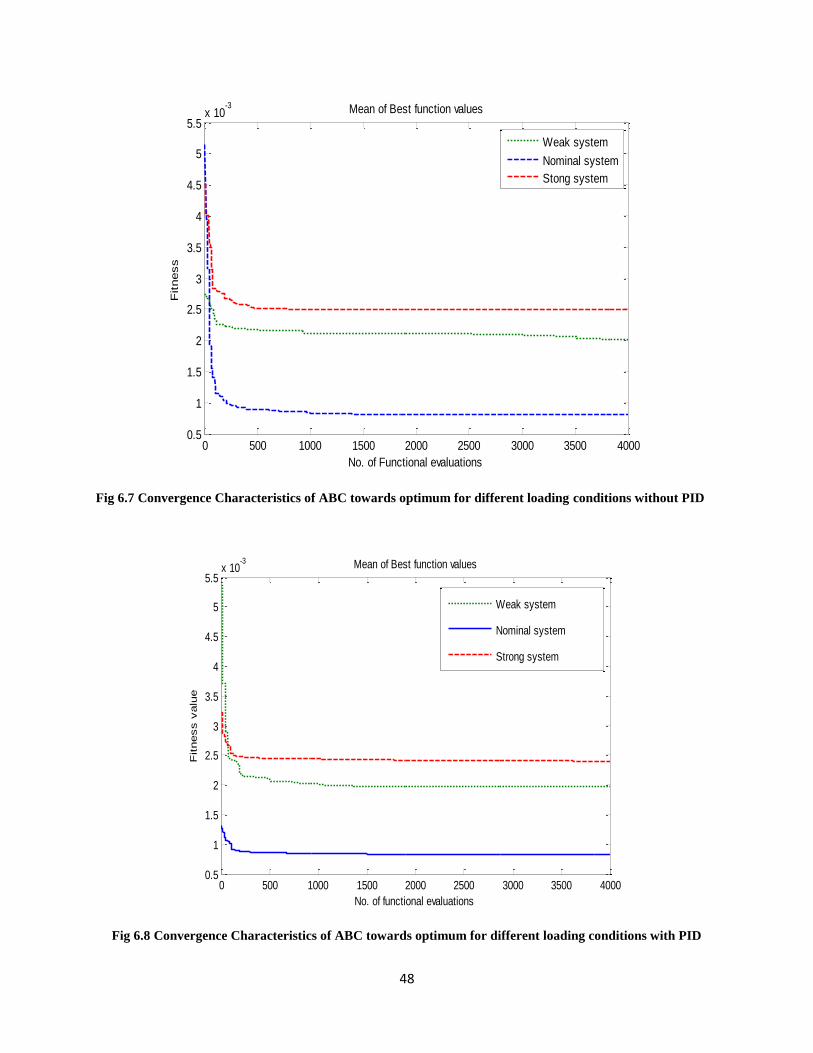
48

Fig 6.7 Convergence Characteristics of ABC towards optimum for different loading conditions without PID

Fig 6.8 Convergence Characteristics of ABC towards optimum for different loading conditions with PID

0 500 1000 1500 2000 2500 3000 3500 40000.5

1

1.5

2

2.5

3

3.5

4

4.5

5

5.5x 10

-3 Mean of Best function values

No. of Functional evaluations

Fitness

Weak system

Nominal system

Stong system

0 500 1000 1500 2000 2500 3000 3500 40000.5

1

1.5

2

2.5

3

3.5

4

4.5

5

5.5x 10

-3 Mean of Best function values

No. of functional evaluations

Fitness v

alu

e

Weak system

Nominal system

Strong system

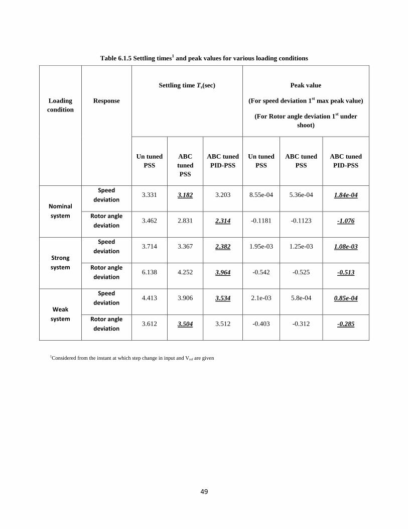
49

Table 6.1.5 Settling times1 and peak values for various loading conditions

Loading

condition

Response

Settling time Ts(sec)

Peak value

(For speed deviation 1st max peak value)

(For Rotor angle deviation 1st under

shoot)

Un tuned

PSS

ABC

tuned

PSS

ABC tuned

PID-PSS

Un tuned

PSS

ABC tuned

PSS

ABC tuned

PID-PSS

Nominal

system

Speed

deviation 3.331 3.182 3.203 8.55e-04

5.36e-04

1.84e-04

Rotor angle

deviation 3.462 2.831 2.314 -0.1181 -0.1123 -1.076

Strong

system

Speed

deviation 3.714 3.367 2.382 1.95e-03 1.25e-03 1.08e-03

Rotor angle

deviation 6.138 4.252 3.964 -0.542 -0.525 -0.513

Weak

system

Speed

deviation 4.413 3.906 3.534 2.1e-03

5.8e-04

0.85e-04

Rotor angle

deviation 3.612 3.504 3.512 -0.403 -0.312 -0.285

1Considered from the instant at which step change in input and Vref are given

50

6.2 Simulations for coordinated tuned PI controllers of TCSC-PSS for SMIB

system using ABC algorithm:

In this context we considered three different loading conditions and they are as follows:

i. Nominal Loading: Pe=1.0, Qe=0.303.

ii. Light Loading: Pe=0.3, Qe=0.015 and system inertia reduces by 25%.

iii. Heavy Loading: Pe=1.01, Qe=0.1 and total line reactance increases by 30%.

For a step change of 5% in input (Pm), in Fig 6.9-6.14 the responses obtained for nominal,

heavy and light loaded systems are depicted in terms of speed deviation and rotor angle

deviations. The optimum parametric values of coordinated tuned TCSC-PSS controllers and

coordinated PI controllers for TCSC and PSS are recorded in tables 6.2.1 and 6.2.2 respectively.

Table 6.2.1: Parametric Values Obtained for coordinated

TCSC- PSS Using ABC and Obj func. Minimization values

Parameter Nominal

Loading

Heavy

Loading

Light

Loading

KTCSC 30.0000 30.0000 30.0000

T1T 0.4226 0.4185 0.1000

T2T 0.2778 0.2394 0.1912

T3T 0.3428 0.1000 0.2532

T4T 0.3940 0.2067 0.2568

KPSS 30.0000 30.0000 30.0000

T1P 0.3076 0.2198 0.2482

T2P 0.1960 0.3138 0.2733

T3P 0.1021 0.2163 0.1811

T4P 0.3921 0.3353 0.1678

Obj Fun without

PI mean(std)

1.7684e-04

(1.300e-07)

1.9699e-04

(4.394e-07)

1.9932-03

(1.125e-08)

51

Table 6.2.2: Parametric Values Obtained for coordinated PI controller TCSC- PSS Using ABC and obj func. Minimization values

Parameter Nominal System Heavy System Light System

KP_TCSC 4.3709 5.2020 2.6232

Ki_TCSC 10.0000 10.0000 10.0000

KP_PSS 0.6785 3.6136 4.8863

Ki_PSS 10.0000 10.0000 10.0000

Obj Fun with mean(std) 4.2233e-05

(1.136e-07)

5.0702e-05

(2.4243e-07)

5.29012e-05

(9.71640e-09)

Fig 6.9 Speed deviation response for Heavy loaded system

0 1 2 3 4 5 6 7 8 9 10-6

-4

-2

0

2

4

6

8x 10

-4

time (sec)

Speed d

evia

tion

PSO-PSS

PSO tuned TCSC-PSS

ABC tuned TCSC-PSS

ABC tuned PI based TCSC-PSS

52

Fig 6.10 Rotor angle deviation response for Heavy loaded system

Fig 6.11 Speed deviation response for Light loaded system

0 1 2 3 4 5 6 70

0.02

0.04

0.06

0.08

0.1

0.12

0.14

0.16

time (sec)

roto

r angle

devia

tion

PSO - PSS

PSO tuned TCSC-PSS

ABC tuned TCSC-PSS

ABC tuned PI basedTCSC-PSS

0 1 2 3 4 5 6 7-5

0

5

10x 10

-4

time (sec)

speed d

evia

tion

PSO - PSS

PSO tuned TCSC-PSS

ABC tuned TCSC-PSS

ABC tuned PI based TCSC-PSS

53

Fig 6.12 Rotor Angle Deviation: Light loaded

Similarly Fig 6.11 and 6.12 show the speed deviation and rotor angle deviation responses for

lightly loaded system. As expected proposed PI based ABC tuned coordinated TCSC-PSS

controller has shown less settling times for both speed and rotor angle deviation responses.

Unlike heavy loaded system, this system enriched with coordinated controllers gave less the less

peak over shoots for both rotor angle and speed deviation responses.

Fig 6.13 and 6.14 depict the speed deviation and rotor angle deviations for the nominal

loaded system. PI based TCSC-PSS controller tuned with ABC algorithm has shown relatively

less settling times and less peak over shoot values for both speed and rotor angle deviation

responses.

0 1 2 3 4 5 6 70

0.02

0.04

0.06

0.08

0.1

0.12

0.14

0.16

time (sec)

roto

r angle

devia

tion

PSO-PSS

PSO tuned TCSC-PSS

TLOBA tuned TCSC-PSS

TLOBA tuned PI based TCSC-PSS

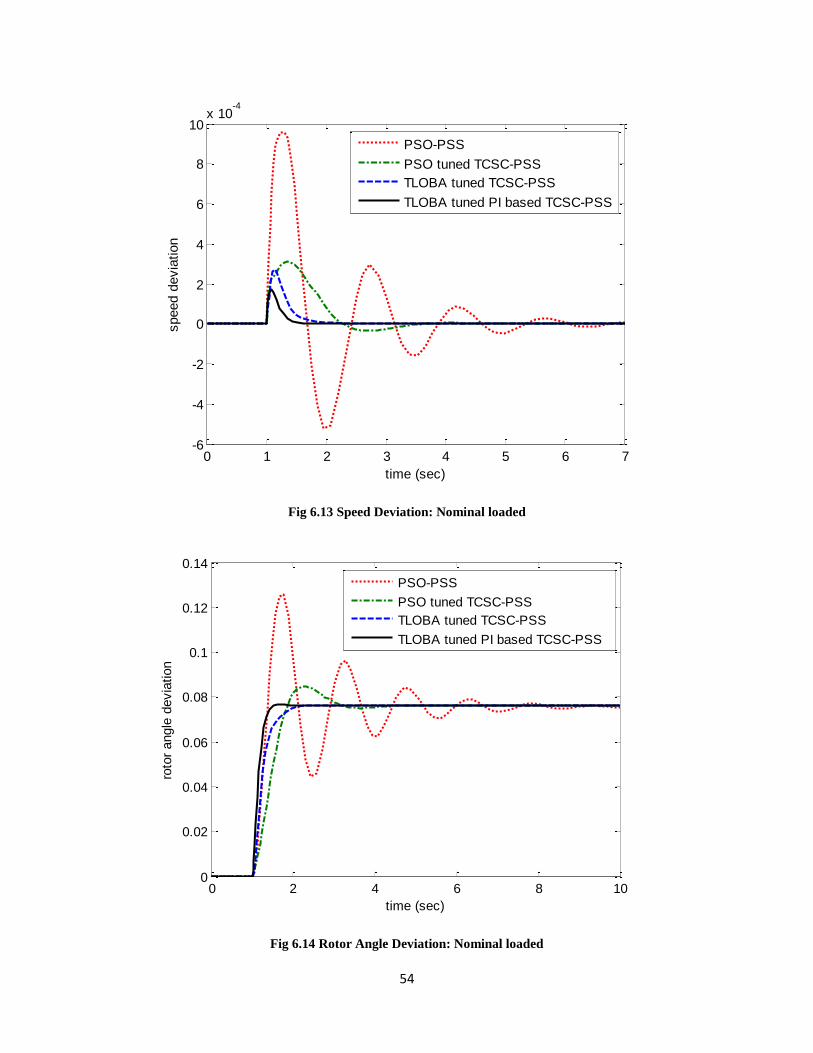
54

Fig 6.13 Speed Deviation: Nominal loaded

Fig 6.14 Rotor Angle Deviation: Nominal loaded

0 1 2 3 4 5 6 7-6

-4

-2

0

2

4

6

8

10x 10

-4

time (sec)

speed d

evia

tion

PSO-PSS

PSO tuned TCSC-PSS



0 2 4 6 8 100

0.02

0.04

0.06

0.08

0.1

0.12

0.14

time (sec)

roto

r angle

devia

tion

PSO-PSS

PSO tuned TCSC-PSS



55

Finally Fig 6.15 and 6.16 show the convergence characteristics of ABC algorithm towards

optimum values without and with PI controllers respectively.

Fig 6.15 Convergence of ABC towards minimum: without PI Controller

Fig 6.16 Convergence of ABC towards minimum: with PI Controller

The parameters obtained via optimal tuning are recorded in Table 6.2.1 and Table 6.2.2.

From both the tables it is further evident that objective function value is less for the PI controller

0 50 100 150 2001.6

1.8

2

2.2

2.4

2.6

2.8x 10

-4

Number of Function Evaluations

Obje

ctive F

unction (

In L

og s

cale

)

NOMINAL SYSTEM

LIGHT LOADED SYSTEM

HEAVY LOADED SYSTEM

0 50 100 150 2000.4

0.6

0.8

1

1.2

1.4

1.6x 10

-4


Obje

ctive F

unction (

In L

og s

cale

)

NOMINAL SYSTEM

LIGHT LOADED SYSTEM

HEAVY LOADED SYSTEM

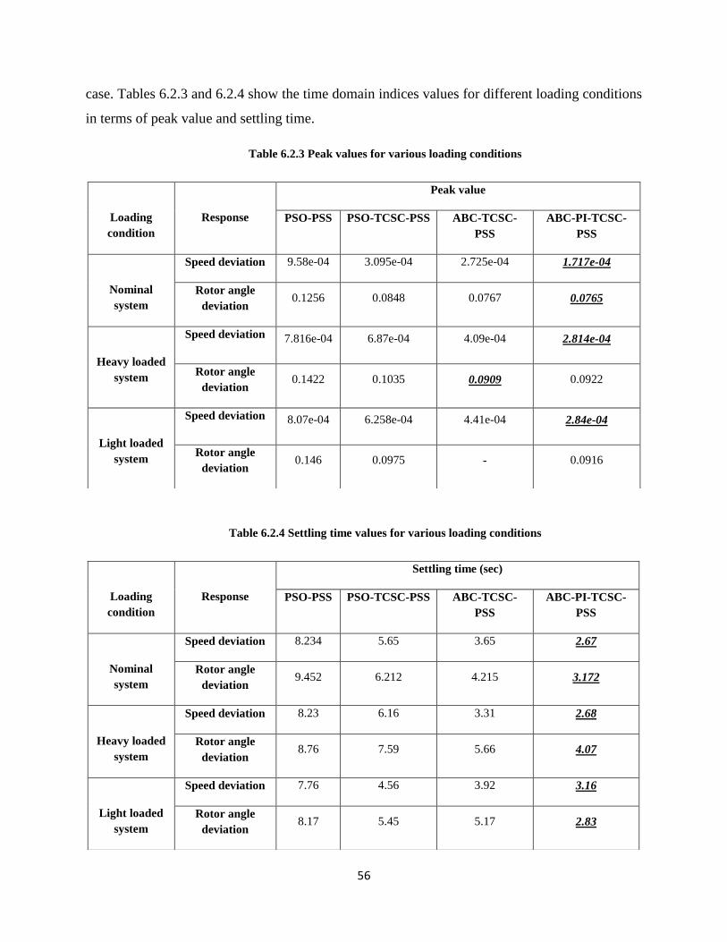
56

case. Tables 6.2.3 and 6.2.4 show the time domain indices values for different loading conditions

in terms of peak value and settling time.

Table 6.2.3 Peak values for various loading conditions

Table 6.2.4 Settling time values for various loading conditions

Loading

condition

Response

Peak value

PSO-PSS PSO-TCSC-PSS ABC-TCSC-

PSS

ABC-PI-TCSC-

PSS

Nominal

system

Speed deviation 9.58e-04

3.095e-04

2.725e-04

1.717e-04

Rotor angle

deviation 0.1256 0.0848 0.0767 0.0765

Heavy loaded

system

Speed deviation 7.816e-04 6.87e-04 4.09e-04

2.814e-04

Rotor angle

deviation 0.1422 0.1035 0.0909 0.0922

Light loaded

system

Speed deviation 8.07e-04

6.258e-04

4.41e-04

2.84e-04

Rotor angle

deviation 0.146 0.0975 - 0.0916

Loading

condition

Response

Settling time (sec)

PSO-PSS PSO-TCSC-PSS ABC-TCSC-

PSS

ABC-PI-TCSC-

PSS

Nominal

system

Speed deviation 8.234 5.65 3.65 2.67

Rotor angle

deviation 9.452 6.212 4.215 3.172

Heavy loaded

system

Speed deviation 8.23 6.16 3.31 2.68

Rotor angle

deviation 8.76 7.59 5.66 4.07

Light loaded

system

Speed deviation 7.76 4.56 3.92 3.16

Rotor angle

deviation 8.17 5.45 5.17 2.83

57

6.3 Simulations for coordinated tuned PI controllers of UPFC damping

controllers for SMIB system using ABC algorithm

In this context we considered three different loading conditions and they are as follows:

Table 6.3.1 Loading conditions considered (p.u)

Nominal Loading

Ps=1.0, Qs=0.015

Heavy Loading

Ps=0.3,Qs=0.015

Light Loading

Ps=1.1 ,Qs=0.4

Parametric values of damping controllers obtained for nominal loading condition using ABC

algorithm are tabulated as follows.

Table 6.3.2 Parametric values of damping controllers obtained for Nominal loaded system using ABC

Nominal Loading

Individual tuned

Controllers

Coordinated tuned

Controllers

Parameter mB E mB E

Kp 100.00 - 67.131 66.220 -30.794

T1 0.7296 4.9085 2.4397 0.1000

T2 0.1000 1.3271 4.1891 2.6803

T3 5.0000 1.9279 1.9907 0.1000

T4 3.0012 0.9410 0.1000 0.6432

58

Table 6.3.3 Parametric values of coordinated PI controllers obtained for nominal loaded system using ABC

Parametric values of damping controllers obtained for nominal loading condition using ABC

algorithm are tabulated as follows.

Table 6.3.4 Parametric values of damping controllers obtained for light loaded system using ABC

Table 6.3.5 Parametric values of coordinated PI controllers obtained for light loaded system using ABC

Coordinated tuned PI Controllers (nominal loaded system)

Parameter mB E

Kp 1.9321 2.3451

Ki 8.9751 1.6324

Light Loading

Individual tuned

Controllers

Coordinated tuned

Controllers

Parameter mB B mB B

Kp 94.665 -87.817 72.366 -100.0

T1 1.3786 3.1720 0.6982 5.0000

T2 0.1000 3.4658 0.1000 1.1660

T3 5.0000 4.9345 4.2977 5.0000

T4 2.9590 0.1000 0.9675 1.4053

Coordinated tuned PI Controllers (light loaded system)

Parameter mB E

Kp 3.2654 3.8479

Ki 7.6545 1.3487

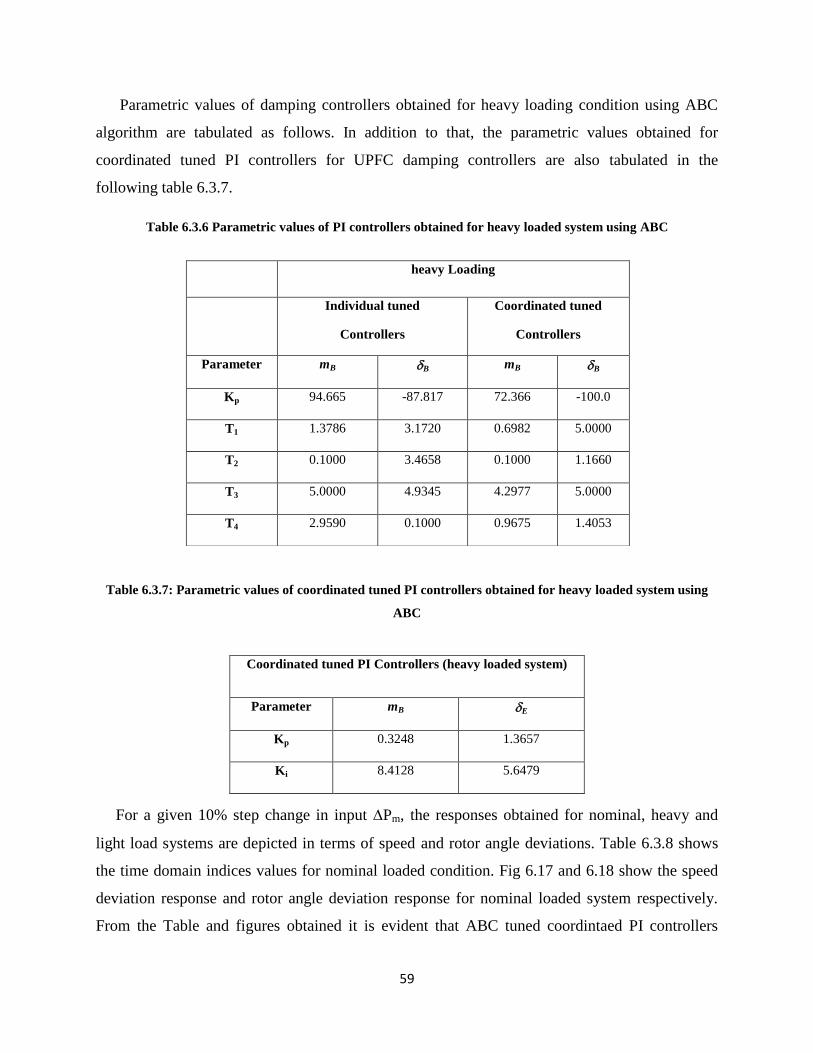
59

Parametric values of damping controllers obtained for heavy loading condition using ABC

algorithm are tabulated as follows. In addition to that, the parametric values obtained for

coordinated tuned PI controllers for UPFC damping controllers are also tabulated in the

following table 6.3.7.

Table 6.3.6 Parametric values of PI controllers obtained for heavy loaded system using ABC

Table 6.3.7: Parametric values of coordinated tuned PI controllers obtained for heavy loaded system using

ABC

For a given 10% step change in input Pm, the responses obtained for nominal, heavy and

light load systems are depicted in terms of speed and rotor angle deviations. Table 6.3.8 shows

the time domain indices values for nominal loaded condition. Fig 6.17 and 6.18 show the speed

deviation response and rotor angle deviation response for nominal loaded system respectively.

From the Table and figures obtained it is evident that ABC tuned coordintaed PI controllers

heavy Loading

Individual tuned

Controllers

Coordinated tuned

Controllers

Parameter mB B mB B

Kp 94.665 -87.817 72.366 -100.0

T1 1.3786 3.1720 0.6982 5.0000

T2 0.1000 3.4658 0.1000 1.1660

T3 5.0000 4.9345 4.2977 5.0000

T4 2.9590 0.1000 0.9675 1.4053

Coordinated tuned PI Controllers (heavy loaded system)

Parameter mB E

Kp 0.3248 1.3657

Ki 8.4128 5.6479

60

based UPFC damping controllers have shown the optimum system performance for nominal

loaded system.

Table 6.3.8 Time domain indices for speed and rotor angle deviation responses and objective function

minimization values for nominal loaded system

Nominal System

Speed deviation Rotor angle deviation

1st Peak over

shoot

settling time

(sec)

1st Peak

over shoot

settling

time (sec)

Obj fun. Mean (std)

PSO – PSS[1] 2.07e-03 NaN 0.24 NaN -

PSO – mB[1] 1.54e-03 7.72 0.26 7.38 -

PSO - E[1] 1.726e-03 9.58 0.246 9.53 -

ABC – mB 1.219e-03 4.32 0.115 4.76 4.68e-04 (6.91e-07)

ABC - E 1.656e-03 4.45 0.278 5.88 7.97e-04(2.72e-06)

ABC CoormB -E 1.101e-03 4.26 0.106 5.23 3.79e-04(2.56e-07)

ABC CoorPImB -E 8.9e-04 3.75 0.0975 2.36 1.45e-04(3.46e-09)

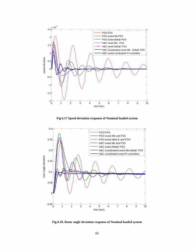
61

Fig 6.17 Speed deviation response of Nominal loaded system

Fig 6.18. Rotor angle deviation response of Nominal loaded system

0 1 2 3 4 5 6 7 8 9 10-2

-1.5

-1

-0.5

0

0.5

1

1.5

2

2.5x 10

-3

time (sec)

speed d

evia

tion

PSO-PSS

PSO tuned Mb-PSS

PSO tuned deltaE-PSS

ABC tuned Mb - PSS

ABC tuned DeltaE PSS

ABC Coordinated tuned Mb - DeltaE PSS

ABC tuned coordinated PI controllers

0 1 2 3 4 5 6 7 8 9 10-0.05

0

0.05

0.1

0.15

0.2

0.25

0.3

time (sec)

roto

r angle

devia

tion

PSO-PSS

PSO tuned Mb and PSS

PSO tuned delta E and PSS

ABC tuned Mb and PSS

ABC tuned DeltaE PSS

ABC Coordinated tuned Mb-DeltaE PSS

ABC coordinated tuned PI controllers

62

Fig 6.19 and 6.20 show the speed deviation response and rotor angle deviation response

for light loaded system respectively. From the table 6.3.9 and figures it is evident that ABC

tuned coordintaed PI controllers based UPFC damping controllers have shown the optimum

system performance for light loaded system.

Table 6.3.9. Time domain indices for speed and rotor angle deviation responses and objective function

minimization values for light loaded system

Light loaded System


1st Peak over

shoot

settling time

(sec)

1st Peak

over shoot

settling

time (sec)

Obj fun. Mean (std)

PSO – PSS[1] 3.409e-03 NaN 0.362 NaN

PSO – mB[1] 2.484e-03 9.76 0.335 9.24

PSO - E[1] 2.761e-03 7.73 0.458 7.58

ABC – mB 2.094e-03 5.01 0.416 7.42 7.73e-04(2.86e-05)

ABC - E 2.681e-03 7.04 0.168 6.59 6.04e-03(3.23e-03)

ABC CoormB -E 1.657e-03 3.46 0.166 8.62 6.06e-04(2.73e-05)


63

Fig 6.19. Speed deviation response of Light loaded system

Fig 6.20. Rotor angle deviation response of light loaded system

0 1 2 3 4 5 6 7 8 9 10-3

-2

-1

0

1

2

3

4x 10

-3

time (sec)

speed d

evia

tion

PSO-PSS

PSO tuned Mb-PSS

PSO tuned DeltaB-PSS

ABC tuned Mb - PSS

ABC tuned Delta-B PSS

ABC coordinated tuned Mb - Delta-B PSS

ABC coordinated tuned PI controllers

0 1 2 3 4 5 6 7 8 9 100

0.05

0.1

0.15

0.2

0.25

0.3

0.35

0.4

0.45

0.5

time (sec)

err

or

PSO-PSS

PSO tuned Mb-PSS

PSO tuned DeltaB-PSS

ABC tuned Mb - PSS

ABC tuned DeltaE - PSS

ABC Coordinated tuned Mb - DeltaE PSS

ABC coordinated PI controllers

64

Fig 6.21 and 6.22 show the speed deviation response and rotor angle deviation response for

heavy loaded system respectively. From the Table 6.3.10 and Fig 6.21-6.22 it is evident that

ABC tuned coordintaed PI controllers based UPFC damping controllers have shown the

optimum system performance for heavy loaded system

Table 6.3.10.Time domain indices for speed and rotor angle deviation responses and objective function

minimization values for heavy loaded system

Heavy loaded System


1st Peak over

shoot

settling time

(sec)

1st Peak

over shoot

settling

time (sec)

Obj fun. Mean (std)

PSO – PSS[1] 3.81e-03 9.96 0.674 9.63

PSO – mB[1] 2.02e-03 6.74 0.627 8.76

PSO - E[1] 5.11e-03 9.35 1.249 9.54

ABC – mB 1.76e-03 5.29 0.462 8.38 2.691e-03(4.38e-05)

ABC - E 4.47e-03 6.58 0.89 8.24 9.471e-03(6.49e-03)

ABC CoormB -E 1.60e-03 5.25 0.367 7.82 1.111e-03(8.69e-06)


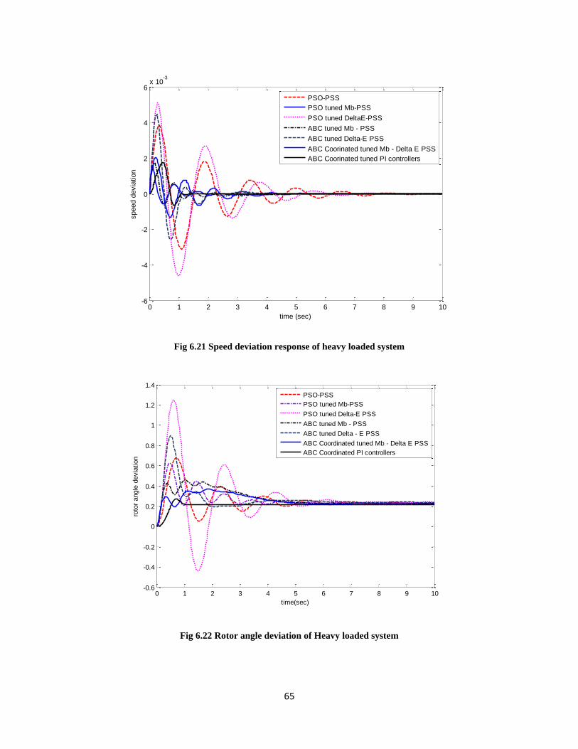
65

Fig 6.21 Speed deviation response of heavy loaded system

Fig 6.22 Rotor angle deviation of Heavy loaded system

0 1 2 3 4 5 6 7 8 9 10-6

-4

-2

0

2

4

6x 10

-3

time (sec)

speed d

evia

tion

PSO-PSS

PSO tuned Mb-PSS

PSO tuned DeltaE-PSS

ABC tuned Mb - PSS

ABC tuned Delta-E PSS

ABC Coorinated tuned Mb - Delta E PSS

ABC Coorinated tuned PI controllers

0 1 2 3 4 5 6 7 8 9 10-0.6

-0.4

-0.2

0

0.2

0.4

0.6

0.8

1

1.2

1.4

time(sec)

roto

r angle

devia

tion

PSO-PSS

PSO tuned Mb-PSS

PSO tuned Delta-E PSS

ABC tuned Mb - PSS

ABC tuned Delta - E PSS

ABC Coordinated tuned Mb - Delta E PSS

ABC Coordinated PI controllers

66

Fig 6.23-6.25 show the object function minimization plots for heavy, nominal and light loaded

systems respectively.

Fig 6.23 Objective function minimization plot for heavy loaded system

Fig 6.24. Objective function minimization plot for nominal loaded system

0 20 40 60 80 100 120 140 160 180 2001

2

3

4

5

6

7

8

9

10

11x 10

-3


Fitness V

alu

e

ABC tuned Mb

ABC tuned Delta-E

ABC tuned coordinated Mb - Delta-E

0 20 40 60 80 100 120 140 160 180 2000

0.5

1

1.5

2

2.5

3

3.5

4

4.5x 10

-3


Fitness V

alu

e

ABC tuned Mb

ABC tuned Delta-E

data3ABC tuned Coordinated MB-DeltaE

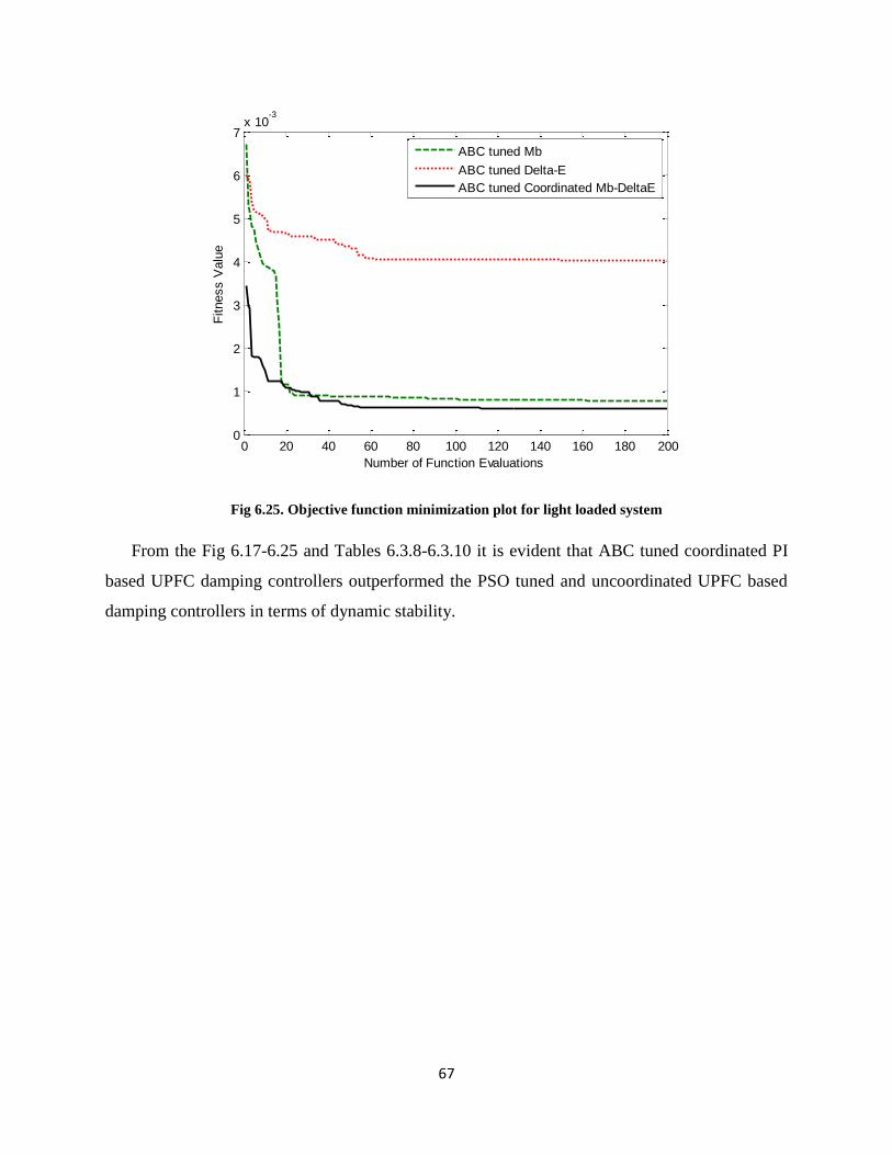
67

Fig 6.25. Objective function minimization plot for light loaded system

From the Fig 6.17-6.25 and Tables 6.3.8-6.3.10 it is evident that ABC tuned coordinated PI

based UPFC damping controllers outperformed the PSO tuned and uncoordinated UPFC based

damping controllers in terms of dynamic stability.

0 20 40 60 80 100 120 140 160 180 2000

1

2

3

4

5

6

7x 10

-3


Fitness V

alu

e

ABC tuned Mb

ABC tuned Delta-E

ABC tuned Coordinated Mb-DeltaE

68

Conclusions

In this dissertation modeling of modified Philip-Heffron model is done for carrying out small

signal studies on a single machine infinite bus (SMIB) power system. Flexible AC transmission

systems (FACTS) based controllers i.e., Thyristor Controller Series Compensators (TCSC),

Unified Power Flow Controllers (UPFC) and their hybrid version employing PI/PID controllers

are considered for enhancing the dynamic stability of SMIB. Tuning of controllers has been done

based on time domain optimization frame work with the help of Artificial Bee Colony (ABC)

algorithm. Various loading conditions are also considered to simulate the actual real world

environment. From the above experimental section followed by results and analysis for different

loading conditions indicated the superiority of proposed method. Further this intelligent method

proved to be better than existing traditional methods such as PSS, PI-PSS.

Scope of Future Work

Future works can be directed towards design of FACTS controllers based on Multi Objective

Optimization levied with various design criteria such as avoiding large control signals from the

controllers. An online adaptive methods involving co-ordinated controllers design will be quite

challenging than offline methodology. To improve the stability further, controllers employing

fractional nature such as PID can also be implemented. The problem will be quite complex and

interesting if a 3-machine system is considered.

69

List of Publications from this Dissertation

[1] B. Sreenivas Theja, A. Rajasekhar and D.P. Kothari, ―An intelligent coordinated design of

UPFC based power system stabilizer for dynamic stability enhancement of SMIB power

system‖, 2012 IEEE International Conference on Power Electronics, Drives and Energy Systems

(PEDES-2012), 16-19 Dec. 2012.

[2] B. Sreenivas Theja, A. Rajasekhar, D.P. Kothari and Swagatam Das, ―Design of PID

controller based Power System Stabilizer using a Modified Philip-Heffron‘s Model: An Artificial

Bee Colony Approach‖, 2013 Swarm Intelligence Symposium (SIS) under IEEE SSCI 2013,

Singapore (In Press).

[3] B. Sreenivas Theja, A. Rajasekhar and A. Abraham, ―An Optimal Design of Coordinated PI

based PSS with TCSC Controller using Modified Teaching Learning Based Optimization‖ 2013

IEEE Congress on Evolutionary Computation, CEC-2013, Mexico (Accepted).

[4] B. Sreenivas Theja, A. Raviteja, A. Rajasekhar and A. Abraham, ―Coordinated Design of

PSS with TCSC Controller: An Artificial Bee Colony Approach‖ 2012 IEEE International

Conference on Communication Systems and Network Technologies, CSNT 2012, pp. 606-611,

IEEE Press.

[5] B. Sreenivas Theja, A. Rajasekhar, K. Vamsi Krishna and Y. Chandrasekhar, ― Application

of Multi Objective GA in designing PID controller based PSS for Single Machine Infinite Bus

power system using Modified Philip-Heffron‘s model‖ 2013 IEEE INDICON (to be submitted)

70

Appendix

A. Glossary

Pm, P (Pe) Mechanical input power and electrical output power of the generator

M, H Machine inertia coefficient and inertia constant

D Machine damping coefficient

id, iq d- and q-axis armature current

vd, vq d- and q-axis terminal voltage

Tdo’ Open-circuit field time constant

xd, xd’ d-axis reactance and d-axis transient reactance‘s.

xq Generator q-axis reactance

V or v Generator terminal voltage

Eq', Efd Generator internal and field voltages

Vref Reference voltage

vb: Infinite bus voltage

KA, TA Gain and time constant of the excitation system

uPSS PSS control signal

Ks, Ts FACTS gain and time constant

mE, mB Excitation and boosting amplitude modulation ratios

vEt, iE Excitation voltage and current

vBt, iB Boosting voltage and current

Cdc, vdc DC link capacitance and voltage

xE, xB ET and BT reactance‘s

Ksyn, Kd Synchronizing and damping torques

δ Rotor angle

ω Rotor speed

ωb Synchronous speed

δE Excitation phase angle modulation

δB Boosting phase angle modulation

δS Voltage angle at secondary of Transformer bus

71

VS and S Voltage and voltage angle at secondary transformer

Firing angle of Thyristor

B. Acronyms Used in this Dissertation

SMIB: Single-machine infinite bus

PSS: Power system stabilizer

AVR: Automatic Voltage Regulator

FACTS: Flexible AC transmission systems

TCSC: Thyristor-controlled series capacitor

UPFC: Unified Power Flow Controller

POD: Power Oscillation Damping

VSC: Voltage Source Converter

p.u: Per Unit

ABC: Artificial Bee Colony

SCR: Silicon Controlled Rectifier

72

C. SIMULINK MODELS

Fig C.1 Liner Philip-Heffron’s model of SMIB employing PI based UPFC Damping Controllers

Fig C.2 Liner Philip-Heffron’s model of SMIB employing Coordinated PI Controllers for TCSC and PSS

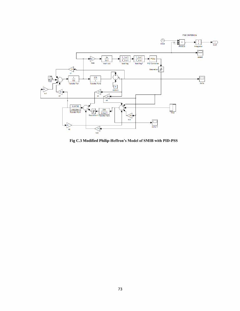
73

Fig C.3 Modified Philip-Heffron’s Model of SMIB with PID-PSS

74

REFERENCES

[1] F. de Mello and C. Concordia, ―Concepts of synchronous machine stability as affected by

excitation control‖, IEEE Transactions on Power Apparatus and Systems, Vol. 88, pp. 316-329,

1969.

[2] E. V. Larsen and D. A. Swann; ―Applying power system stabilizers,‖ IEEE Transactions on

Power Apparatus and Systems, Vol. 100, No. 6, pp. 3017-3046, 1981.

[3] G. Gurrala and I. Sen, "A Modified Heffron-Phillip's Model for The Design of Power System

Stabilizers‖, IEEE Power India Conference and Joint International Conference on Power

System Technology, 2008. POWERCON 2008, pp.1-6, Oct. 2008.

[4] M. A. Abido, “Robust design of multi machine power system stabilizers using simulated

annealing‖, IEEE Transactions on Energy Conversion , Vol. 15 Issue. 3 , pp. 297 -304, Sept.

2000.

[5] M. A. Abido, “Particle swarm optimization for multi machine power system stabilizer

design‖, IEEE Power Engineering Society Summer Meeting, 2001. Vol. 3, pp. 1346 -1351, 15-19

July 2001.

[6] M. A. Abido and Y. L. Abdel-Magid,” Robust design of electrical power-based stabilizers

using tabu search‖, Power Engineering Society Summer Meeting. IEEE , Vol. 3 pp. 1573 -1578,

15-19 July 2001.

[7] S. Dechanupaprittha and I. Ngamroo, ―Design of robust power system stabilizers in a multi

machine power system using tabu search algorithm‖, IEEE International Conference on

Industrial Technology, ICIT 2002, Vol. 1 , pp. 291 -296, 11-14 Dec. 2002.

[8] N. G. Hingorani, “High Power Electronics and flexible AC Transmission System‖, Power

Engineering Review, IEEE, Vol. 8 Issue. 7, pp. 3-4, July 1988.

[9] N. G. Hingorani, ―FACTS technology and opportunities, Flexible AC Transmission Systems

(FACTS) - The Key to Increased Utilisation of Power Systems‖, IEE Colloquium on (Digest

No.1994/005), pp. 4/1-410, 12 Jan 1994.

75

[10] P. Sidhartha and N. P. Padhya ―Coordinated Design of TCSC Controller and PSS

Employing Particle Swarm Optimization Technique‖ International Journal of Computer and

Information Engineering, 1(5), 2007.

[11] AlAwami, Ali Taleb. ― Design of Robust PSS and facts-based controllers for stability

enhancement of power systems - .by Ali Taleb Al-Awami‖ /. 2004.

[12] I. Manuaba, M. Abdillah, Soeprijanto and M. P. Henry, "Coordination of PID based power

system stabilizer and AVR using combination of bacterial foraging technique – Particle swarm

optimization,‖ 4th International Confernce on Modeling, Simulation and Applied Optimization

(ICMSAO), pp. 1-7, April 2011.

[13] Y.L. Abdel-Magid, M. Bettayeb and M.M. Dawoud, ―Simultaneous stabilization of power

systems using genetic algorithms‖ in IEE Proceedings Generation Transmission Distribution,

vol. 144, No. 1, pp. 39-44, January 1997.

[14] B. Selvabala, D. Devaraj, ―Co-ordinated tuning of AVR-PSS using differential evolution

algorithm,‖ In Proceedings: IPEC, 2010, pp.439-444, Oct. 2010.

[15] R. Vikal and G.Goyal, "TCSC Controller Design Using Global Optimization for Stability

Analysis of Single Machine Infinite-Bus Power System," 15th

International Conference on

Intelligent System Applications to Power Systems, 2009. ISAP '09, pp.1-7.

[16] N. Magaji and M. W. Mustafa, "TCSC Damping controller design based on Self-learning

fuzzy controller Techniques," 5th

International Power Engineering and Optimization Conference

(PEOCO), 2011 pp.387-391, 6-7 June 2011.

[17] R. Narne and P. C. Panda and J. P. Therattil, "Transient stability enhancement of SMIB

system using PSS and TCSC-based controllers," IEEE Ninth International Conference on Power

Electronics and Drive Systems (PEDS), 2011, pp. 214-218.

[18] S. Panda, R. N. Patel and N. P. Padhya, ―Power System Stability Improvement by TCSC

Controller Employing a Multi- Objective Genetic Algorithm Approach‖, International Journal

of Electrical and Computer Engineering 1:8 2006.

76

[19] H F Wang. ‗A Unified Model for the Analysis of FACTS Devices in DampingPower

System Oscillations — Part III : Unified Power Flow Controller.‘ IEEE Transactions on Power

Delivery, vol 15, no 3, p. 978, July 2000.

[20] K. R. Padiyar, and A.M. Kulkarni, ―Control design and simulation of unified power flow

controller,‖ IEEE Transactions on Power Delivery , vol.13, no.4, pp.1348-1354, Oct 1998.

[21] Tambey, N.; Kothari, M.L.; , "Damping of power system oscillations with unified power

flow controller (UPFC)," IEE Proceedings Generation, Transmission and Distribution, 150(2)

pp. 129- 140, March 2003.

[22] J. Guo and ML. Crow, ―An improved UPFC control for oscillation damping,‖ IEEE Trans.

Power Syst., 25(1), pp. 288–296, 2009.

[23] C. D. Schauder, L. Gyugyi, M. R. Lund, D. M. Hamai, T. R. Rietman, D. R. Torgerson, and

A. Edris, ―Operation of the unified power flow controller (UPFC) under practical constraints,‖

IEEE Trans. Power Delivery, vol. 13, pp. 630–636, Apr. 1998.

[24] D. Karaboga and B. Basturk, ―A powerful and efficient algorithm for numerical function

optimization: artificial bee colony (abc) algorithm‖, J Glob Optim 39(3): pp. 459-471.

[25] B. Bastruk and D. Karaboga, ―An artificial bee colony (abc) algorithm for numeric function

optimization,‖ In: IEEE Swarm intelligence symposium 2006, Indianapolis, IN, USA.

[26] D. Karaboga and B. Akay, ―A survey: algorithms simulating bee swarm intelligence,‖

Artificial Intelligence Review. 31(1-4), pp. 61-85.

[27] S. Hemamalini and S. Simon, ―Economic load dispatch with value-point effect using

artificial bee colony algorithm‖ In XXXII national systems conference, India.

[28] S. Hemamalini and S. Simon, ―Economic/Emission Load Dispatch Using Artificial Bee

Colony Algorithm. In Proc: International Conference on Control Communication and Power

Engineering. ACEEE

77

[29] S.N. Omkar, J. Senthilnath, R. Khandelwal, G. Narayan Naik and S. Gopalkrishnan,

―Artificial Bee Colony (ABC) for multi-objective design optimization of composite structures.

Applied Soft Comput. 11(1), pp. 489-499.

[30] Abu-Mouti FS and E-Harway M.E, ―Modified artificial bee colony algorithm for optimal

distributed generation sizing and allocation in distribution systems‖, Electrical Power & Energy

Conference (EPEC), 2009, IEEE,pp. 1-9, 2009.

[31] B. Akay and D. Karaboga, ―Artificial Bee Colony algorithm for large-scale problems and

engineering design optimization. J of Intelligent Manufacturing. Springer. Pp. 1-14, 2010.

[32] D. Karaboga, B. Gorkemli, C. Ozturk and N. Karaboga, ―A Comprehensive survey:

artificial bee colony (ABC) algorithm and applications. Artificial Intelligence Review.

NATIONAL INSTITUTE OF TECHNOLOGY - …arajasekhar.weebly.com/uploads/2/2/5/7/22576192/thesis.pdfAN...

Documents

Transcript of NATIONAL INSTITUTE OF TECHNOLOGY - …arajasekhar.weebly.com/uploads/2/2/5/7/22576192/thesis.pdfAN...