TUBERCULOSIS MODEL: A MATHEMATICAL

ANALYSIS

NADHIRAH BT ABDUL HALIM

FACULTY OF SCIENCE

UNIVERSITY OF MALAYA

KUALA LUMPUR

2013

TUBERCULOSIS MODEL: A MATHEMATICAL

ANALYSIS

NADHIRAH BT ABDUL HALIM

DISSERTATION SUBMITTED IN FULFILMENT OF

THE REQUIREMENTS FOR THE DEGREE OF

MASTER OF SCIENCE

INSTITUTE OF MATHEMATICAL SCIENCES

FACULTY OF SCIENCE

UNIVERSITY OF MALAYA

KUALA LUMPUR

2013

ii

UNIVERSITI MALAYA

ORIGINAL LITERARY WORK DECLARATION

Name of Candidate: Nadhirah bt Abdul Halim I.C/Passport No.: 860331-56-6368

Registration/Matric No: SGP 090005

Name of Degree: Master of Science (Msc.)

Title of Project Paper/Research Report/Dissertation/Thesis (“this Work”):

Tuberculosis Model: A Mathematical Analysis

Field of Study:

I do solemnly and sincerely declare that:

1. I am the sole author/writer of this Work

2. This Work is original

3. Any use of any work in which copyright exists was done by way of fair dealing

and for permitted purposes and any excerpt or extract from, or reference to or

reproduction of any copyright work has been disclosed expressly and

sufficiently and the title of the Work and its authorship have been

acknowledged in this Work;

4. I do not have any actual knowledge nor do I ought reasonably to know that the

making of this work constitutes an infringement of any copyright work;

5. I hereby assign all and every rights in the copyright to this Work to the

University of Malaya (“UM”), who henceforth shall be owner of the copyright

in this Work and that any reproduction or use in any form or by any means

whatsoever is prohibited without the written consent of UM having been first

had and obtained;

6. I am fully aware that if in the course of making this Work I have infringed any

copyright whether intentionally or otherwise, I may be subject to legal action or

any other action as may be determined by UM.

Candidature’s Signature Date

Subscribed and solemnly declared before,

Witness’s Signature Date

Name:

Designation:

iii

ABSTRACT

In this thesis, the design and analysis of compartmental deterministic models for the

transmission dynamics of infectious disease in a population is studied.

A basic Susceptible-Exposed-Infected-Recovered (SEIR) model for the transmission of

infectious disease with immigration of latent and infectious individuals is developed

and rigorously analyzed. The model is assumed to have permanent immunity and

homogenous mixing. The constant immigration of the infected individuals into the

population makes it impossible for the disease to die out which means, there will be no

disease-free equilibrium. However, it is shown that there exists an endemic equilibrium

which is locally asymptotically stable under certain parameters restriction.

We then extend the 3-compartment Susceptible-Exposed-Infected (SEI) tuberculosis

(TB) model with immigration proposed by McCluskey and van den Driessche (MnD)

in 2004 into a 4-compartment SEIR model. The treated individuals are moved into the

recovered group with slight immunity against the TB. Results show the importance of

treatment to the infected and that treatment for the latently infected are more effective

in curbing the disease.

In the last model, we analyze the best approach in containing the spread of the disease

under different factors. We incorporate the idea of immigration into the TB

transmission model with chemoprophylaxis treatment as proposed by Bhunu et al. [3].

The results show that the immigration effects are overwhelmed by the other

contributing factors such as the high rate of re-infection, making it insignificant;

contradicting with reality. Simply giving treatments also does not give the best result

iv

on a long term basis as the population will eventually die out. Different kinds of

intervention are needed to ensure a more successful prevention plan and one way is to

reduce the contact rate of the infectious individuals.

v

ABSTRAK

Tesis ini adalah mengenai reka bentuk dan analisis model kompartmen berketentuan

untuk dinamik penularan penyakit berjangkit dalam sesebuah populasi.

Model asas Rentan-Terdedah-Dijangkiti-Pulih (SEIR) untuk penularan penyakit

berjangkit yang melibatkan imigrasi individual-individual yang terdedah dan terjangkit

dibina dan dianalisis secara teliti. Model ini diandaikan mempunyai imuniti kekal dan

pergaulan seragam. Imigrasi berterusan individu yang berpenyakit ke dalam populasi

menyebabkan mustahil untuk menghapuskan penyakit itu; yakni tidak wujud

keseimbangan bebas-penyakit. Walau bagaimanapun di bawah kekangan parameter

tertentu, dapat ditunjukkan kewujudan suatu titik keseimbangan yang stabil secara

asimptotik tempatan.

Seterusnya, model TB 3-bahagian Rentan-Terdedah-Dijangkiti (SEI) dengan imigrasi

yang dicadangkan oleh McCluskey and van den Driessche (MnD) pada tahun 2004

dikembangkan kepada model 4-bahagian (SEIR). Individu yang dirawat dipindahkan

ke kumpulan yang pulih dengan sedikit imuniti terhadap TB. Hasil kajian menunjukkan

betapa pentingnya rawatan kepada individu yang dijangkiti serta keberkesanan rawatan

terhadap individu yang terdedah kepada penyakit dalam membendung penularan

penyakit.

Model terakhir digunakan untuk menganalisa pendekatan terbaik dalam mengawal

penyebaran penyakit di bawah keadaan berbeza. Idea imigrasi digabungkan ke dalam

model penularan TB dengan rawatan chemoprophylaxis yang diusulkan oleh Bhunu et

al. [3]. Hasil kajian menunjukkan bahawa kesan immigrasi tidak begitu penting

dibandingkan dengan faktor-faktor penyumbang lain seperti kadar jangkitan semula

vi

yang tinggi; ini bertentangan dengan realiti. Setakat memberi rawatan juga tidak

memberi keputusan yang terbaik dalam jangka masa panjang memandangkan seluruh

populasi akan mati juga akhirnya. Pelbagai langkah berbeza perlu diambil untuk

memastikan pelan pencegahan yang lebih berjaya, dan salah satu daripadanya adalah

dengan mengurangkan kadar pertembungan individu yang terjangkit.

vii

ACKNOWLEDGEMENT

This dissertation would not have been possible without the guidance and the help of

several individuals who in one way or another contributed and extended their valuable

assistance in the preparation and completion of this study.

First and foremost, my utmost gratitude goes to my supervisor, Mr. Md. Abu Omar

Awang, for his patience and steadfast encouragement. The supervision and unfailing

support that he gave throughout the whole programme makes the whole process more

bearable.

Assoc. Prof. Dr. Mohd b. Omar, Head of the Department of Institute of Mathematical

Sciences (ISM) for the kind concern regarding my thesis progress;

All academic staff of ISM for the moral support and encouragement;

All non-academic staff of ISM for accommodating to my various queries;

Fellow graduates, especially Miss Noorul Akma bt Amin for her inputs in the

programming part of this study and others for their valuable insights.

Last but not the least, my thanks to my family and friends for being there for me

through this whole journey and the Almighty, Allah that makes all of these possible.

viii

TABLE OF CONTENTS

DECLARATION

ABSTRACT

ABSTRAK

ACKNOWLEDGEMENT

TABLE OF CONTENTS

LISTS OF TABLES

LISTS OF FIGURES

CHAPTER 1 INTRODUCTION

1.1. Introduction

1.2. History of tuberculosis

1.3. Tuberculosis at a glance

1.3.1. What is tuberculosis?

1.3.2. How does a person get TB?

1.3.3. Who gets TB?

1.3.4. What are the symptoms?

1.3.5. Diagnosis of TB

1.3.6. Treatment of TB

1.4. Problem statement

1.5. Aim and objectives

1.6. Organization of thesis

CHAPTER 2 LITERATURE REVIEW

2.1. Introduction

2.2. History of mathematical modelling in

infectious disease

2.3. The epidemic models

2.4. Review of tuberculosis models

CHAPTER 3 METHODOLOGY

3.1. Introduction

3.2. Research design

3.3. Model stability

3.4. Data collection

3.5. Data analysis

Page

ii

iii

v

vii

viii

x

xi

1

1

2

2

3

3

4

4

5

5

6

7

7

8

10

13

13

13

14

ix

3.5.1. Numerical study

3.5.2. Variation of variables and parameter values

CHAPTER 4 THE MODELS

4.1. Introduction

4.2. Basic SEIR model with immigration

4.2.1. Model formulation

4.2.2. The endemic equilibrium

4.2.3. Local asymptotic stability of the endemic

equilibrium

4.2.4. Conclusion

4.3. Extending MnD SEI model into SEIR

model

4.3.1. Model formulation

4.3.2. Numerical study

4.3.3. Conclusion

4.4. Extending Bhunu model

4.4.1. Model formulation

4.4.2. Numerical study

4.4.3. Conclusion

CHAPTER 5 CONCLUSION AND FUTURE

RESEARCH

5.1. Conclusion

5.2. Recommendations for future research

APPENDIXES

APPENDIX A Compound matrices

APPENDIX B MATLAB Programme

BIBLIOGRAPHY

14

15

16

16

20

21

23

24

27

32

33

36

43

44

46

47

48

51

x

LIST OF TABLE

Table Title Page

4.1 Model parameters and their interpretations 27

xi

LIST OF FIGURES

Figure Title Page

4.1 Basic SEIR model structure 17

4.2

A MATLAB plot showing the solutions of system (5)

converge to finite limit 20

4.3 (a) The TB model with immigration proposed by 24

McCluskey and van den Driessche

(b) Our proposed extended SEIR model structure 25

4.4 Phase plane portraits of system (17) using parameter

values in Table 4.1

(a) Susceptible vs. Exposed 26

(b) Susceptible vs. Infectives 26

4.5 (a) A graphical representation showing the trend of 28

all classes for the MnD model

(b) A graphical representation showing the trend of 29

all classes for our extended SEIR model

4.6 (a) MnD model: A graphical simulation when there is 30

no immigration of infected people

(b) SEIR extended model: A graphical simulation when 30

there is no immigration of infected people

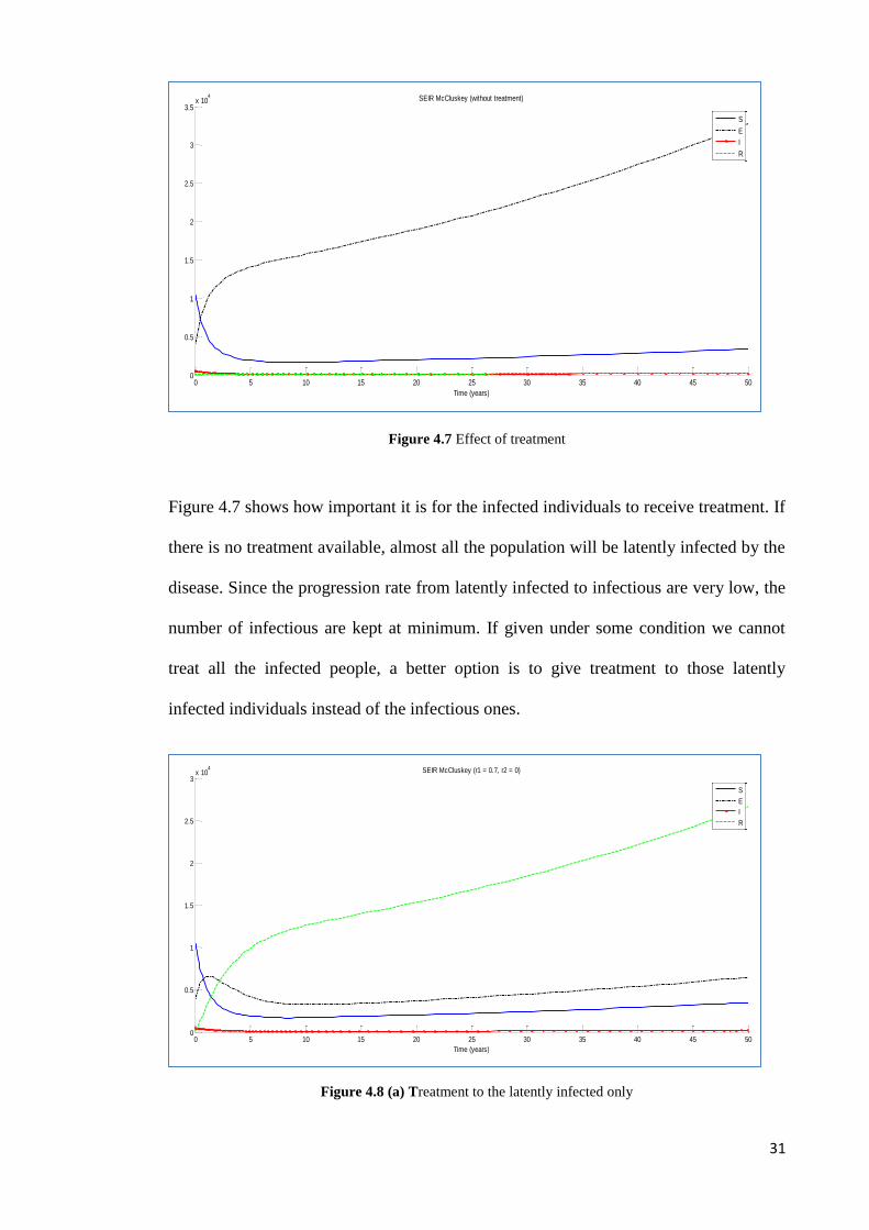
4.7 Effect of treatment 31

4.8 (a) Treatment to the latently infected only 31

(b) Treatment to the infectious only 32

4.9 Structure of model 34

4.10 Phase plane portraits of system (18) using parameter

values in Table 4.1.

(a) Susceptible vs. Exposed 35

(b) Susceptible vs. Infectives 36

xii

Figure Title Page

4.11 A graphical representations showing the trend of all 37

classes for model system (17)

4.12 (a) Model system with a=b=0: The latently infected and 37

infectious class when there is no immigration of

infected individuals

(b) Model system with a= 0.3, b=0.1: The latently infected 38

and infectious class when there is an immigration of

infected individuals

4.13 (a) The susceptible population with and without treatment 39

(b) The latently infected and the infectious population with

and without treatment 39

(c) The recovered population with and without treatment 40

4.14 (a) Model system with c =80 41

(b) Model system with c = 18 42

4.15 Total population with various contact rates, c. 42

1

CHAPTER 1

INTRODUCTION

1.1. Introduction

Tuberculosis (TB) is a worldwide pandemic disease. According to World Health

Organization (WHO), one-third of the world’s population is currently infected by the

TB bacillus bacteria. Being a disease of poverty, the vast majority of TB deaths are in

the developing world with more than half occurring in Asia [28].

The estimated global incidence rate are falling very slowly from the peak of 141 cases

per 100,000 population in 2002 to 128 cases per 100,000 population in 2010. The TB

death rate has also fallen by 40% since 1990 and the number of deaths is also declining.

Globally, the percentage of people successfully treated reached its highest level at 87%

in 2009.

1.2. History of tuberculosis

TB is believed to have been present in humans for thousands of years. Skeletal remains

show that prehistoric humans (4000BCE) had TB and tubercular decay has been found

in the spines of Egyptian mummies dating from 3000-2400 BCE [14, 25]. It was not

identified as a single disease until the 1820s due to the variety of its symptoms. In

1834, Johann Lukas Schonlein gave the disease name ‘tuberculosis’ [14].

Mycobacterium tuberculosis, the bacteria that caused the tuberculosis was identified by

Nobel Laureate Robert Koch in March 1882 and in 1900’s, Albert Calmette and

Camille Guerin achieved the first genuine success in immunizing against tuberculosis

using attenuated bovine-strain tuberculosis called 'BCG' (Bacillus of Calmette and

Guerin) [14]. It was not until 1946 with the development of the antibiotic streptomycin

2

that effective treatment and cure became possible. However, hopes of completely

eliminating the disease were dashed following the rise of drug-resistant strains in the

1980s.

1.3. Tuberculosis at a glance

1.3.1. What is tuberculosis?

Tuberculosis (TB) is an infectious disease caused by Mycobacterium tuberculosis

bacteria. It spreads through the air like the common cold. Most TB infections will

results as a latent infection where the body is able to fight the bacteria and stopping

them from growing. The bacteria thus will become dormant and remain in the body

without causing symptoms.

However, when the immune system of a patient with dormant TB is weakened, the TB

can become active and cause infection in the lungs or other parts of the body. Only

those with active TB can spread the disease. According to WHO, 5-10% of people who

are infected with TB will become infectious at some time during their life and if left

untreated each person will infect on average 10 to 15 people every year [28].

1.3.2. How does a person get TB?

Tuberculosis is spread through the air from one person to another. The bacteria get into

the air when someone who has a tuberculosis lung infection coughs, sneezes, shouts, or

spits [5, 28]. People who are nearby can then possibly breathe the bacteria into their

lungs and become infected. Even though the disease is airborne, it is believed that TB is

not highly infectious and so, occasional contacts with infectious person rarely lead to

infection [26]. TB cannot be spread through handshakes, sitting on toilet seats or

sharing dishes and utensils with someone who has TB.

3

1.3.3. Who gets TB?

It is said that, every second, one person in the world is newly infected with TB bacilli

[28]. Anyone can catch TB, but people who are particularly at risk include

• those who live in close contact with individuals who have an active TB

infection e.g. family members, nurses and doctors,

• those with weak immune system either because of age or health problem e.g.

young children or elderly people, alcoholics, intravenous drug users, patient

with diabetes, certain cancers and HIV, and

• those who live in environments where the level of existing TB infection is

higher than normal e.g. poor and crowded environment, prison inmates,

homeless people.

1.3.4. What are the symptoms?

Symptoms of TB disease depend on where in the body the TB bacteria grow. Active

TB cases may be pulmonary where it affects the lungs. The early symptoms usually

include fatigue or weakness, unexplained weight loss, fever, chills, loss of appetite and

night sweats [5, 28]. Since the symptoms are very much similar to a common cold

people tend to treat it as one. When the infection in the lung worsens, it may cause

chest pain, bad cough that last 3 weeks or longer and coughing up of sputum and/or

blood.

There are also cases where the infection spreads beyond the lungs to other parts of the

body such as the bones and joints, the digestive system, the bladder and reproductive

system and the nervous system. This is known as extra pulmonary TB and the

4

symptoms will depend upon the organs involved. It is more common in people with

weaker immune systems, particularly those with an HIV infection.

1.3.5. Diagnosis of TB

One who came with the symptoms may be suspected with TB based on the patient’s

medical history, medical conditions and physical exam. There are several different

ways to diagnose TB such as analysis of sputum, skin test and chest X-rays.

The skin test is used to identify those who may have been exposed to tuberculosis by

injecting a substance called tuberculin under the skin. A positive test shows that the

person may have been infected but does not necessarily mean they have active TB.

Other tests are done in making a diagnosis of active tuberculosis which includes

identifying the causative organism Mycobacterium tuberculosis in the sputum.

Sometimes, diagnosis may also be made using the chest X-rays by looking at things

such as evidence of active tuberculosis pneumonia, and scarring or hardening in the

lungs.

1.3.6. Treatment of TB

Tuberculosis is treated by killing the bacteria using antibiotics. The treatment usually

last at least 6 months in duration and sometimes longer up to 24 months. It involves

different antibiotics to increase the effectiveness while preventing the bacteria from

becoming resistant to the medicines.

The most common medicines used for active tuberculosis are Isoniazid (INH),

Rifampin (RIF), Ethambutol and Pyrazinamide [5]. People with latent tuberculosis are

usually treated using a single antibiotic to prevent them from progressing to active TB

disease later in life.

5

The successful of tuberculosis treatment is largely dependent on the compliance of the

patient. One of the main reason that cause the failure of TB treatment is because the

patient failed to take the medications as prescribed. In most cases, proper treatment

with appropriate antibiotics will cure the TB. Without treatment, tuberculosis can be a

lethal infection.

1.4. Problem statement

According to World Health Organization (WHO), the number of people falling ill with

TB each year is declining [28]. However, this downward trend is threaten by the

increasing number of TB cases in immigrants especially in countries that have

substantial levels of immigration from areas with a high prevalence of the disease [16,

21]. The immigrants here are generally the people who are travelling from less to more

economically developed geographical areas in search of jobs and better living

conditions. As an air-borne infectious disease, it is impossible for any country to isolate

itself. In long-term, the best defense against TB is to bring the disease under control

worldwide.

1.5. Aim and Objectives

Our aim is to analyze the dynamic of Tuberculosis transmission under different

conditions in order to identify key factors which contribute in the spreading of the

disease using mathematical model.

The objectives of the study are:

To see how immigration plays a role in TB spreading,

To determine how effective the treatment for both latently infected and

infectious individuals in controlling the spread of the disease, and

6

To deduce an action plan for prevention, control and monitoring of TB from the

results obtained.

1.6. Organization of thesis

This thesis is divided into five chapters. Following this introductory Chapter 1,

Chapter 2 is the literature review that surveys previous literature and studies relevant to

our research. Chapter 3 describes and explains the research methodology used. The

sub-topics include the research design, model stability, data collection and data

analysis. In Chapter 4 the models and results are presented. The last chapter, Chapter 5,

is the conclusion from our results and also suggestions for future research. The

bibliography concludes this thesis.

7

CHAPTER 2

LITERATURE REVIEW

2.1. Introduction

In mathematical modeling, we translate our beliefs about how the world functions into

the language of mathematics. A model is a quantified simplification of the complex

reality. The construction of a model involves the formulation of a hypothesis about the

nature of the relationships that exists between the various relevant factors. Its quality

depends on the accuracy of its underlying assumptions.

2.2. History of Mathematical Modelling in Infectious Disease

Mathematical models have become an important tool in analyzing the spread and

control of infectious disease. The results from mathematical models can help in

determining the plausibility of epidemiologic explanations and predicting the impact of

changes on the dynamics of the system. It is important for understanding the population

dynamics of the transmission of infectious agents and the potential impact of infectious

disease control programs [2].

The very first epidemiological model was formulated by Daniel Bernoulli in 1760 [4]

in order to evaluate the impact of variolation on human life expectancy. However,

deterministic epidemiology modelling seems to have started in the 20th

century when

Hamer [13] formulated and analyzed a discrete time model on measles in 1906,

followed by Ross [24] with his work on malaria in 1911.

In 1927, Kermack and McKendrick [18] obtained one of the key results in

epidemiology by deriving the threshold theorem that predicts the critical fraction of

8

susceptible in population that must be exceeded in order for an epidemic outbreak to

occur. Starting in the middle of the 20th

century, mathematical epidemiology showed a

rapid growth. The book on mathematical modelling of epidemiological systems that

was published by Bailey [3] is said to be an important landmark which, in part, led to

the recognition of the importance of modelling in public health decision making [1, 7,

15].

In the epidemiology of tuberculosis, the model approach was first applied by Frost [12].

He predicted in 1937 that with the low and falling rate of transmission of infection in

the United States, it was most likely that the disease will eventually be eradicated. His

prediction was confirmed by Feldman [10] in 1957 by making further progress in

model-making.

Today, variety of models have been formulated, mathematically analyzed and applied

to infectious disease.

2.3. The epidemic models

The fundamental process represented in mathematical model of the epidemiology of

infectious disease is the transmission of infectious agents.

Mathematical models characterize transmission in terms of infection

rates related to the frequency of contact between individuals and the

likelihood of transmission given a contact between a susceptible host

and infective host [2].

This process is represented as a series of stages of infection starting with a susceptible

host who becomes infected. The infected host will be able to transmit the infection to

others when the host becomes infective. The period of time that elapses before an

infected host becomes infective is referred as the latent period. The host will then be

9

removed from the transmission cycle when the host is no longer able to transmit

infection. The removal may be caused by death by infection, acquisition of permanent

immunity or successful treatment.

Compartments with label such as S, E, I and R are often used to represent the

epidemiological classes in a population. The first class is susceptible (S) who can

acquire the infection. The second class is exposed (E) who is in the latent period. Next

class is infective (I) who can transmit infection to susceptible and lastly the class of

recovered (R) who is immune. Acronyms for epidemiology models are often based on

the flow patterns between the compartments such as SEI, SIS, SIR, SEIR, SEIS, SEIRS

to name a few.

The basic reproduction number is the threshold for many epidemiology models. It is

defined as the average number of secondary infections produced when an infected host

is introduced into a fully susceptible population [5, 15]. The threshold quantity is used

to determine when an infection can invade and persist in a new host population.

In some epidemiological models, the incidence rate (the rate of new infections) is

bilinear in the infective fraction I and the susceptible fraction S. Such models usually

have an asymptotically stable trivial equilibrium corresponding to the disease-free state,

or an asymptotically stable nontrivial equilibrium corresponding to the endemic (i.e.

persistent) state depending on the parameter values. However, studies showed that

when the restriction to bilinear incidence rates is dropped, the system can have a much

wider range of dynamical behaviours.

Liu et al [22] studied the dynamical behaviour of epidemiological models with

nonlinear incidence rates. Their studies show that models with nonlinear incidence

have a much wider range of dynamical behaviours than do those with bilinear incidence

rates. For these models, there is a possibility of multiple attractive basins in phase

10

space. Because of that, the disease survival depends not only upon the parameters but

also upon the initial conditions. There are also cases where periodic solutions may

appear by Hopf bifurcation at critical parameter values.

Li and Muldowney [19] studied the SEIR model with nonlinear incidence rates in

epidemiology. The purpose of their paper is to prove the global stability of the

nontrivial equilibrium for their SEIR model. They proved that any periodic orbit of the

system, when it exists, is orbitally asymptotically stable based on a criterion for the

asymptotic orbital stability of periodic orbits for general autonomous systems.

Li et al [20] studied the global dynamics of a SEIR model with varying total population

size. The model assumes that the local density of the total population is a constant

though the total population size may vary with time. They used the homogeneity of the

vector field of the model to analyze the derived system of the fractions (s,e,i,r) in

determining the behaviour of the population sizes (S,E,I,R) and the total population.

The global stability is proved by employing the theory of monotone dynamical systems

together with a stability criterion for periodic orbits of multidimensional autonomous

systems due to Li and Muldowney [19].

2.4. Review of Tuberculosis Models

Internal and international human migration has increased worldwide in recent years.

One of the main factors is because migration was easily done due to improved

transportation. Migrants are generally people travelling from less to more economically

developed geographical areas in search of jobs and better living conditions. With

immigration from areas of high incidence of TB, it is conjectured that this will result in

the resurgence of tuberculosis in areas of low incidence. TB cases involved in

11

immigrants represent a high proportion of the total prevalence rate in many developed

countries [16].

In many developed nations, the main countermeasure in order to reduce the risk of TB

spreading is by the screening of immigrants upon arrival. Nevertheless, several reports

from many developed countries with well-performing screening and treatment systems

have shown in the last few years that foreign-born TB patients do not significantly

contribute to M. tuberculosis transmission to the native population [11, 17].

McCluskey and van den Driessche [23] investigate a SEI TB model with immigration

that includes infected (both latent and infectious) individuals [Figure 4.3 (a)]. The

model assumed constant recruitment with fixed fraction entering each class.

McCluskey and van den Driessche [23] have proved that under certain restrictions on

the parameters (including the treatment rates, disease transmission rate and TB induced

death rate) the disease will approach a unique endemic level. The immigration of

infected results in the disease never dies out and the usual threshold condition found in

many epidemic models is not applicable.

Jia et al [16] investigate the impact of immigration on the transmission dynamics of

tuberculosis. They too incorporated the recruitment of the latent and infectious

immigrants but their model regards the immigrants as a separate subpopulation from

the local population. Their theoretical analysis indicated that the disease will persist in

the population if there is a prevalence of TB in immigrants. They also showed that the

disease never dies out and becomes endemic in host areas. The usual threshold

condition does not apply and a unique equilibrium exists for all parameter values. The

study suggests that immigrants have a considerable influence on the overall

transmission dynamics behaviour of tuberculosis.

12

Both studies show that when there is an immigration of infected into the population,

there will be no disease-free equilibrium. Most study of the model with immigration

will focused on the endemic equilibrium and its stability, and sometimes is supported

by the numerical simulations. Such is the case with McCluskey and van den Driessche

[23] as their paper is focused on the global stability of the model. They first show the

existence of a unique endemic equilibrium using Descartes’ Rule of Signs. Then they

proved its local stability followed by the geometric approach developed in [18] that

involves generalizations of Bendixsons’ Condition to higher dimensions, to prove its

global stability.

Bhunu et al [5] presented a SEIR tuberculosis model which incorporated treatment of

infectious individuals and chemoprophylaxis (treatment for the latently infected). The

model assumed that the latently infected individuals develop active disease as a result

of endogenous re-activation, exogenous re-infection and disease relapse. The study

shows that treatment of infectious individuals is more effective in the first years of

implementation as it cleared active TB immediately. As a result, chemoprophylaxis will

do better in controlling the number of infectious due to reduced progression to active

TB.

From these studies, we can conclude that immigration does have an effect on the spread

of tuberculosis in such a way that the disease persist in the host population [16, 23].

However, with proper treatments and intervention, the rate of infection from

immigrants has little effect to the host population [11, 17]. Further studies are required

to determine which factor plays the bigger role in the spreading of tuberculosis in order

to maintain the balance and keeping the disease under control. This will be part of our

current study.

13

CHAPTER 3

METHODOLOGY

3.1. Introduction

This thesis involved three mathematical model of tuberculosis. For the first model, we

present the analytical part of the model, focusing on the stability of its equilibrium. The

second and third model is used to investigate the dynamic of Tuberculosis transmission

under different condition. We determined the effect of immigration and treatment and

hence deducing an action plan for prevention, control and monitoring of TB.

3.2. Research Design

The research will mainly base its findings through both quantitative and qualitative

research methods as this will allow a flexible and iterative approach. Qualitative

research method was used as we try to find and build theories that will explain the

relationship of one variable with another. Using this method, we are able to interpret

our results and relate it with the real world.

3.3. Model Stability

Our first model is a basic SEIR model [Equation 1(a-e), Figure 4.1] where we

attempted to study and prove its endemic equilibrium stability. The system was reduced

to a sub-system of 3 equations by using the homogeneity characteristic of the system.

The equilibrium points are determined and its local stability is proved using the method

of first approximation. We showed the Jacobian of the matrix system is stable under

certain parameter restrictions, using a Lemma proposed by Li and Muldowney [19].

We have attempted to prove the global stability of our model using the geometric

14

approach as proposed by Li and Muldowney [19]. However, we have not succeeded in

applying this particular technique to obtain the global stability.

3.4. Data Collection

When we first started, we intend to use real data for our study. Later we discovered that

it is an uphill task to get the permission from the Ministry of Health Malaysia,

Department of Immigration Malaysia and also the hospitals that can provide us with the

needed data. Thus, the data used in our research was taken from Bhunu et al. [5]. From

the literature reviews, it is safe to say that the values are acceptable and commonly used

for TB cases in general.

3.5. Data Analysis

3.5.1. Numerical Study

The numerical study is done with the aid of MATLAB. MATLAB is a high-level

language and interactive environment for algorithm development, data visualization,

data analysis and numeric computation that enables one to perform computationally

intensive tasks faster. We solved our model using the built-in-function ode45 which is

an algorithm program based on Runge-Kutta-Fehlberg.

The Runge–Kutta–Fehlberg method (or Fehlberg method) is an algorithm developed by

the German mathematician Erwin Fehlberg and is based on the class of Runge–Kutta

methods. It is often referred to as an RKF45 method as it uses an O(h4) method together

with an O(h5) method that uses all of the points of the O(h

4) method. The method’s

procedure helps to determine if the proper step size h is being used. At each step, two

different approximations for the solution are made and compared. If the two answers

are in close agreement, the approximation is accepted. If the two answers do not agree

15

to a specified accuracy, the step size is reduced. If the answers agree to more

significant digits than required, the step size is increased.

3.5.2. Variation of Variables and Parameter Values

In order to investigate the dynamics of TB transmission under different condition, we

assigned different values of variables and parameters accordingly. The values are

varied systematically to find the critical point of the disease spread under each

condition if any. Qualitative method was then used to explain and interpret the results

and to relate it with the real world.

16

CHAPTER 4

THE MODELS

4.1. Introduction

In this chapter, we presented 3 models for analysis: one basic model and two extended

models. The first model is a basic SEIR model with immigration factor. For the basic

model, we are only interested in the analytical part of the model; hence we present the

analysis on the stability of the endemic equilibrium.

The second model is an extended model based on TB model with immigration as

proposed by McCluskey and van den Driessche [23] and we denote it as MnD model.

We extend their SEI model into a SEIR model and analyze its numerical simulation.

We then compare the results between the SEI and SEIR model. The purpose of this

model is to analyze the effect of immigration and also the effectiveness of the

treatment.

The third model is a model where we incorporate the idea of immigration as proposed

by McCluskey and van den Driessche [23] into the tuberculosis transmission model

with chemoprophylaxis of Bhunu et al. [5]. We use numerical simulations of the model

to illustrate the behaviour of the system. This model is used to analyze the best

approach in containing the spread of the disease under different factors.

4.2. Basic SEIR Model with Immigration

4.2.1. Model formulation

The SEIR model for the spread of TB disease with immigration is described by the

following system of differential equations

17

)1(

)1()(

)1()(

)1()()1(

dRpIdt

dR

cIpdkENbdt

dI

bEkSNadt

dE

aSNbadt

dS

with initial condition

0)0(,0)0(,0)0( 000 IIEESS and )1(.0)0( 0 eRR

Here, the model is divided into four classes: susceptible individuals ,S individuals

exposed to TB (latently infected) E , infected (infectious) individuals ,I and recovered

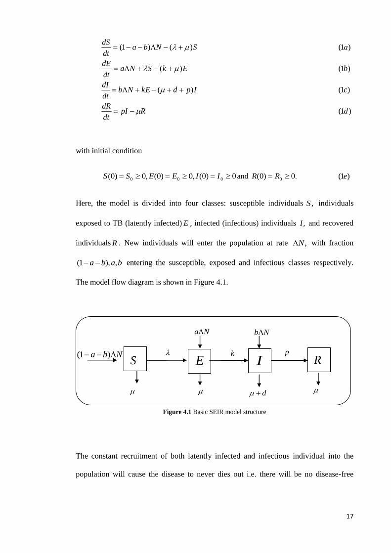
individuals R . New individuals will enter the population at rate ,N with fraction

baba ,),1( entering the susceptible, exposed and infectious classes respectively.

The model flow diagram is shown in Figure 4.1.

Figure 4.1 Basic SEIR model structure

The constant recruitment of both latently infected and infectious individual into the

population will cause the disease to never dies out i.e. there will be no disease-free

Nba )1(

Na

p

R

Nb

d

IE

Sk

18

equilibrium, and therefore no usual threshold condition. We assume that the local

density of the total population is a constant though the total population size

)2()()()()()( tRtItEtStN

may vary with time.

The incidence rate is described by the non-linear term

)3(,/ NIc

where is the transmission probability and c is the per capita contact rate. The natural

death rate in each class is assumed to be a constant and an individual may recover

naturally at rate p .We also assume homogeneous mixing and the infectious

individuals suffer disease-caused mortality with a constant rate, .d Note that those who

recovered, however, will acquire a permanent immunity.

The total population size )(tN can also be determined from the following differential

equation

)4(,)( dINdt

dN

which is derived by adding up all the equations in (1).

Let NIiNEeNSs /,/,/ and NRr / denote the fractions of the classes S, E,

I, R, in the population respectively. It is easy to verify that s, e, i and r satisfy the

system of differential equations

)5('

)5()('

)5()('

)5()()1('

2

ddirrpir

cdiipdkebi

bdieekcisae

aiscdsbas

19

subject to restriction 1 ries . Note that the total population size )(tN does not

appear in (5). This is a direct result of the homogeneity of the system (1). Observe also

that the variable r does not appear in the first three equations of (5). This allows us to

attack (5) by studying the subsystem

)6()('

)6()('

)6()()1('

2 cdiipdkebi

bdieekcisae

aiscdsbas

and determining r from )(1 iesr or

)7(' dirrpir

We study (6) in the closed set

)8(}10|),,{( 3 iesies

where 3

denotes the non-negative cone of 3 including its lower dimension faces. It

can be verified that is positively invariant with respect to (6).

We then established that (6) is a competitive system when dc , which is an

important property in the study of the global dynamics when the disease persists. We

follow the definition and condition of a competitive system given by Li et al [20].

Let nxfx )( be a smooth vector field defined for a in an open set nD . The

differential equation

)9(),(' Dxxfx

is said to be competitive in D if, for some diagonal matrix ),....,( 1 ndiagH where

each i is either 1 or -1, HxfH / has non-positive off diagonal elements for all

Dx . By choosing the matrix H as )1,1,1( diagH , one can verify that, when

dc , the system (6) is competitive in the convex region with respect to the

partial ordering defined by the orthant }0,0,0|),,{( 3 iesies .

20

4.2.2. The endemic equilibrium

The coordinates of an equilibrium point ),,( **** iesP satisfy

)10(0)(

)10(0)(

)10(0)()1(

2 cdiipdkeb

bdieekcisa

aiscdsba

and also 0,0 ** es and 0* i .

Adding the above equations leads to

***** )()1)(( ipiesdi

which gives the following range of *i .

)11(}.,1min{0 *

di

*s and *e can be uniquely determined from *i by

*

*

)(

)1(

icd

bas

and

))((

)1()(***

***

dikcidi

cibdiaae

(12)

respectively.

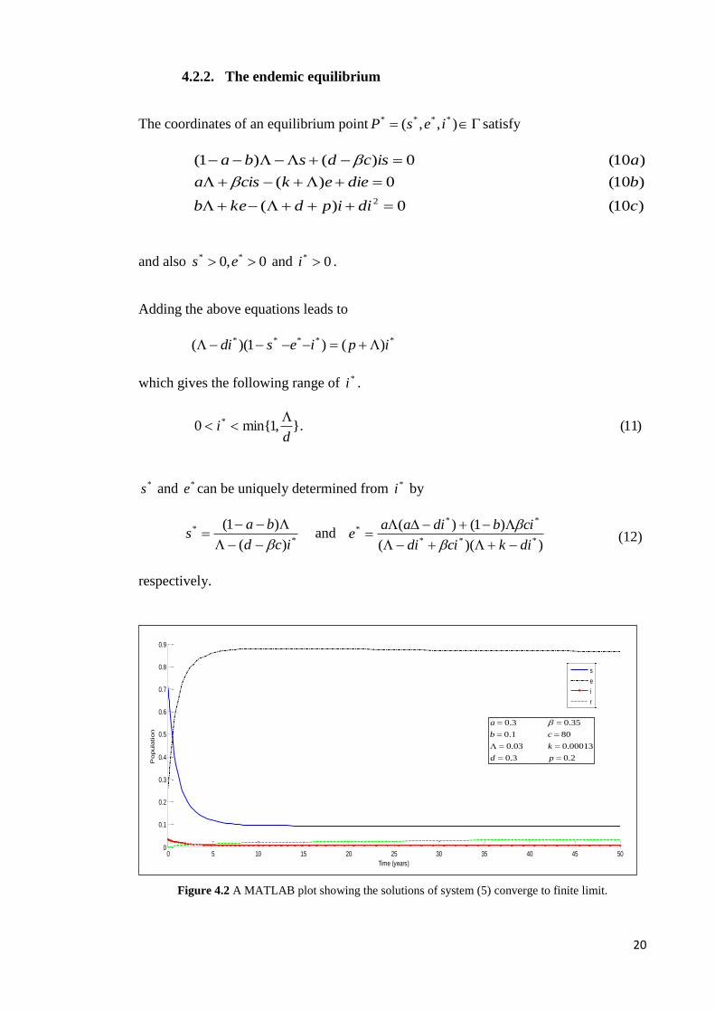
Figure 4.2 A MATLAB plot showing the solutions of system (5) converge to finite limit.

0 5 10 15 20 25 30 35 40 45 500

0.1

0.2

0.3

0.4

0.5

0.6

0.7

0.8

0.9

Time (years)

Popula

tion

s

e

i

r

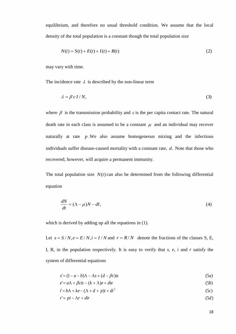
2.03.0

00013.003.0

801.0

35.03.0

pd

k

cb

a

21

Figure (4.2) shows the numerical solution of system (5) that presents the existence of

the globally asymptotically stable endemic equilibrium.

4.2.3. Local asymptotic stability of the endemic equilibrium

The method of first approximation is used to show the asymptotic stability of the

equilibrium ,*P by proving that the matrix )( *PJ is stable i.e. all its eigenvalues have

negative real part.

The Jacobian matrix of (6) at a point ),,( iesP is

)13(

)(20

)(

)(0)(

)(

pddik

decskdici

scdicd

PJ

The following lemma ([Lemma 5.1, Li et al [20]] is used to demonstrate the local

stability of *P .

Lemma. Let A be an mm matrix with real entries. For A to be stable, it is necessary

and sufficient that

1. The second compound matrix ]2[A is stable

2. 0)det()1( Am

Proof. We have to show that )(PJ satisfies both condition given in the Lemma. The

second additive compound )(]2[ PJ of the Jacobian matrix )(PJ is given by

)14(

)2(30

0)2()3(

)()2()2(

)(]2[

kpddici

pdicdk

icddecskicd

PJ

22

For ),,( **** iesP and the diagonal matrix ),,( *** seidiagE , the matrix )( *]2[ PJ is

similar to 1*]2[ )( EPEJ

)2(3*

0

0)2()3(

)(*

)2()2(

)(

*

*

*

*

*

*

**

*

**

1*]2[

kpddie

sci

pdicdi

ke

icddie

scikicd

EPEJ

The matrix )( *]2[ PJ is stable if and only if the 1*]2[ )( EPEJ is stable, for similarity

preserves the eigenvalues. Since the diagonal elements of the matrix 1*]2[ )( EPEJ are

negative, an easy argument using Gersgorin discs shows that it is stable if it is

diagonally dominant in rows.

Set },,max{ 321 ggg where

)2(3

)15()2()3(

)2(2

*

***

3

*

*

*

2

*

***

1

kpde

scidig

pdicdi

keg

e

scikdig

Equation (10) can be written as

*

*

*

*

*

*

*

**

*

*

)16(

)()1(

i

bdipd

i

ke

e

adik

e

sci

idcs

ba

23

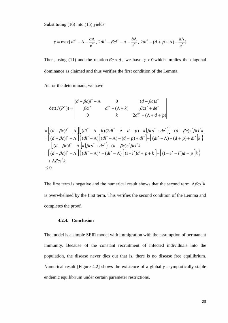
Substituting (16) into (15) yields

})(2,2,max{*

*

*

**

*

*

e

apddi

i

bcidi

e

adi

Then, using (11) and the relation dc , we have 0 which implies the diagonal

dominance as claimed and thus verifies the first condition of the Lemma.

As for the determinant, we have

0

)1()1()()()(

)()(

)()()()()()(

)()2()()(

)(20

)(

)(0)(

))(det(

*

****2**

*****

******

*******

*

****

**

*

kcs

kpdiekpdididiicd

kciscddecskicd

kdipddidipddidiicd

kciscddecskpddikdiicd

pddik

decskdici

scdicd

PJ

The first term is negative and the numerical result shows that the second term kcs*

is overwhelmed by the first term. This verifies the second condition of the Lemma and

completes the proof.

4.2.4. Conclusion

The model is a simple SEIR model with immigration with the assumption of permanent

immunity. Because of the constant recruitment of infected individuals into the

population, the disease never dies out that is, there is no disease free equilibrium.

Numerical result [Figure 4.2] shows the existence of a globally asymptotically stable

endemic equilibrium under certain parameter restrictions.

24

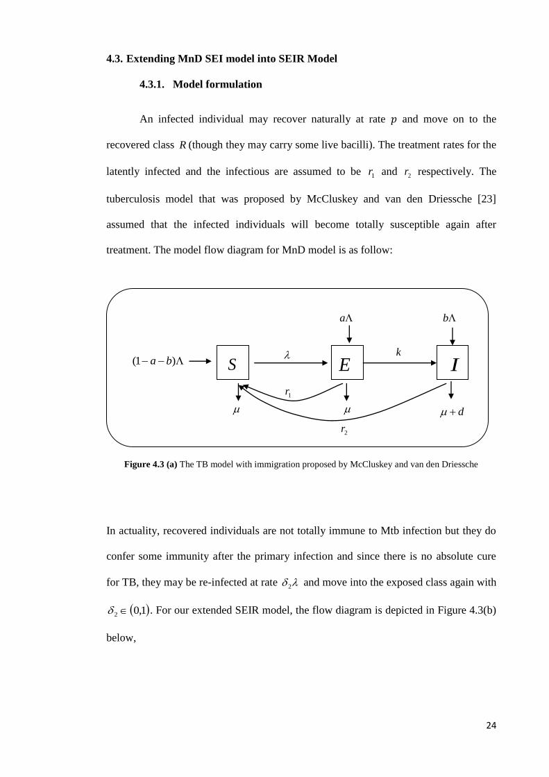
4.3. Extending MnD SEI model into SEIR Model

4.3.1. Model formulation

An infected individual may recover naturally at rate and move on to the

recovered class R (though they may carry some live bacilli). The treatment rates for the

latently infected and the infectious are assumed to be 1r and 2r respectively. The

tuberculosis model that was proposed by McCluskey and van den Driessche [23]

assumed that the infected individuals will become totally susceptible again after

treatment. The model flow diagram for MnD model is as follow:

Figure 4.3 (a) The TB model with immigration proposed by McCluskey and van den Driessche

In actuality, recovered individuals are not totally immune to Mtb infection but they do

confer some immunity after the primary infection and since there is no absolute cure

for TB, they may be re-infected at rate 2 and move into the exposed class again with

1,02 . For our extended SEIR model, the flow diagram is depicted in Figure 4.3(b)

below,

S E I

a

d

b

k )1( ba

1r

2r

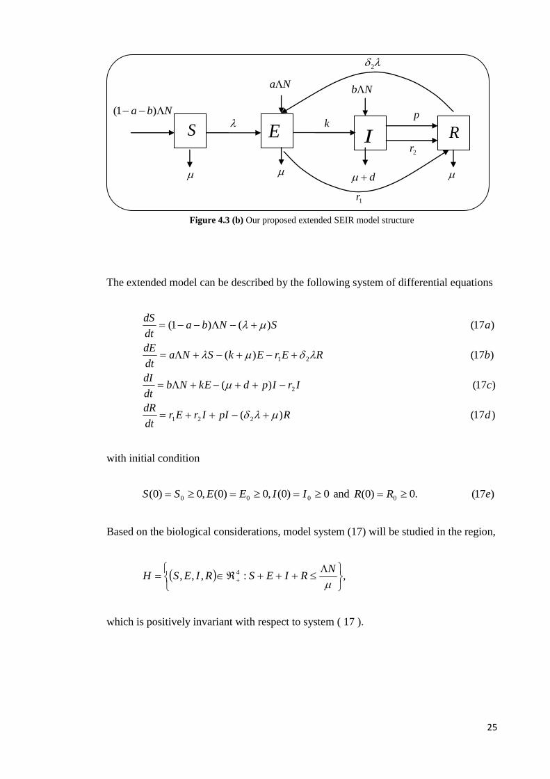
25

Figure 4.3 (b) Our proposed extended SEIR model structure

The extended model can be described by the following system of differential equations

)17()(

)17()(

)17()(

)17()()1(

221

2

21

dRpIIrErdt

dR

cIrIpdkENbdt

dI

bRErEkSNadt

dE

aSNbadt

dS

with initial condition

0)0(,0)0(,0)0( 000 IIEESS and )17(.0)0( 0 eRR

Based on the biological considerations, model system (17) will be studied in the region,

,:,,, 4

NRIESRIESH

which is positively invariant with respect to system ( 17 ).

S E I

Na

d

Nb

k

2

Nba )1(

1r

2r

R

p

26

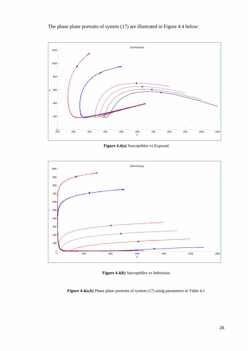
The phase plane portraits of system (17) are illustrated in Figure 4.4 below:

Figure 4.4(a) Susceptibles vs Exposed

Figure 4.4(b) Susceptibles vs Infectious

Figure 4.4(a,b) Phase plane portraits of system (17) using parameters in Table 4.1

1000 2000 3000 4000 5000 6000 7000 8000 9000 10000 110000

2000

4000

6000

8000

10000

12000SEIR McCluskey

S

E

0 2000 4000 6000 8000 10000 120000

1000

2000

3000

4000

5000

6000

7000

8000

9000

10000SEIR McCluskey

S

I

27

4.3.2. Numerical study

In this section, the numerical simulations for the model systems under different

conditions are presented. Note that McCluskey and van den Driessche [23] paper are

focused on the global stability of the model. They did not present any numerical

solutions of their model. We compare our model and theirs using the parameter values

given in Table 4.1 and the initial conditions are taken to be

500)0(,500,3)0(,000,11)0( IES and .0)0( R

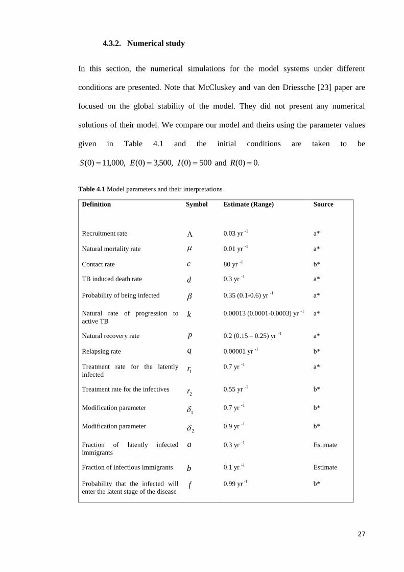
Table 4.1 Model parameters and their interpretations

Definition

Symbol Estimate (Range) Source

Recruitment rate 0.03 yr -1

a*

Natural mortality rate 0.01 yr -1

a*

Contact rate c 80 yr -1

b*

TB induced death rate d 0.3 yr -1

a*

Probability of being infected 0.35 (0.1-0.6) yr -1

a*

Natural rate of progression to

active TB k 0.00013 (0.0001-0.0003) yr

-1 a*

Natural recovery rate p 0.2 (0.15 – 0.25) yr -1

a*

Relapsing rate q 0.00001 yr -1

b*

Treatment rate for the latently

infected 1r 0.7 yr

-1 a*

Treatment rate for the infectives 2r 0.55 yr

-1 b*

Modification parameter 1 0.7 yr

-1 b*

Modification parameter 2 0.9 yr

-1 b*

Fraction of latently infected

immigrants

a 0.3 yr -1

Estimate

Fraction of infectious immigrants b 0.1 yr -1

Estimate

Probability that the infected will

enter the latent stage of the disease f 0.99 yr

-1 b*

28

The parameters values are taken from Bhunu et al. [5] who also relied on the values

taken from Dye and William [8] and Dye et al. [9], aside from their own estimations. In

Table 4.1, a* denotes parameter values and ranges adapted from Dye and William [8],

Dye et al. [9] and b* denotes the parameter values from Bhunu et al. [5].

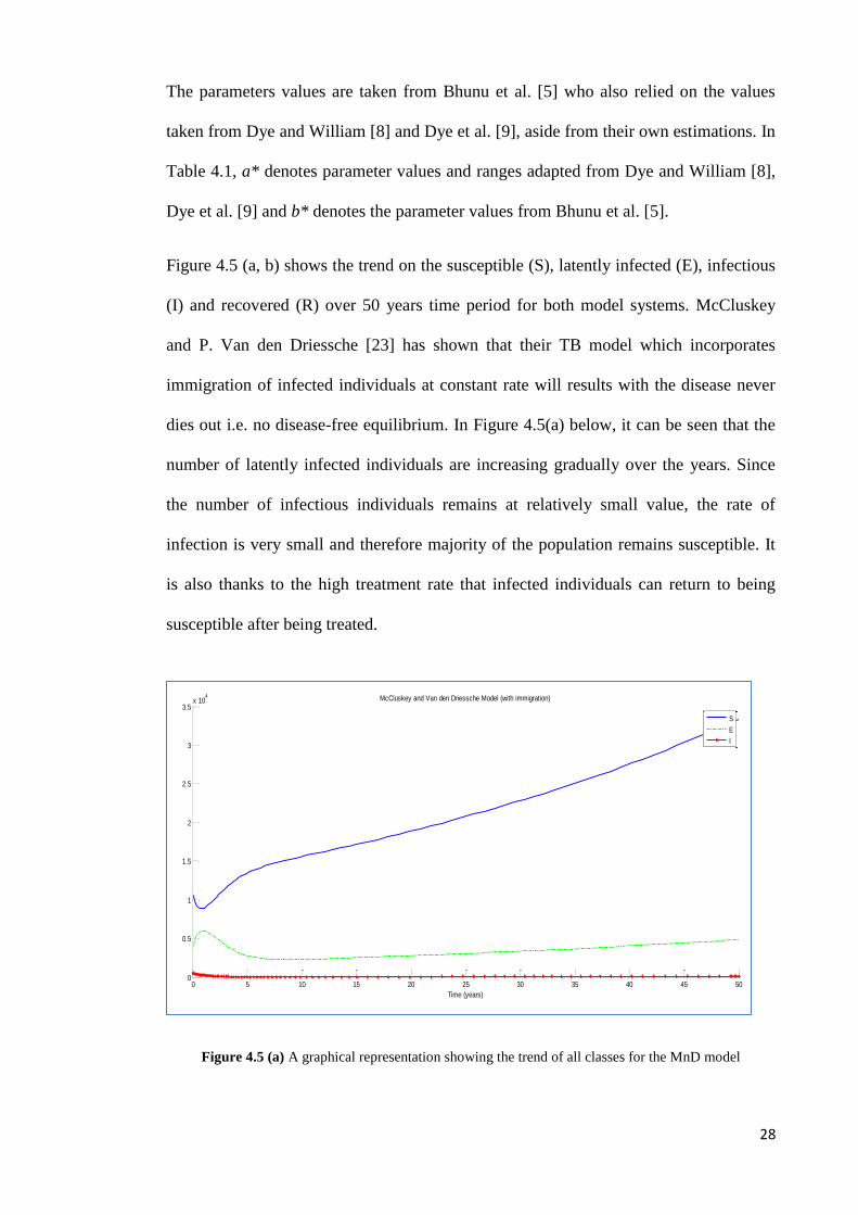
Figure 4.5 (a, b) shows the trend on the susceptible (S), latently infected (E), infectious

(I) and recovered (R) over 50 years time period for both model systems. McCluskey

and P. Van den Driessche [23] has shown that their TB model which incorporates

immigration of infected individuals at constant rate will results with the disease never

dies out i.e. no disease-free equilibrium. In Figure 4.5(a) below, it can be seen that the

number of latently infected individuals are increasing gradually over the years. Since

the number of infectious individuals remains at relatively small value, the rate of

infection is very small and therefore majority of the population remains susceptible. It

is also thanks to the high treatment rate that infected individuals can return to being

susceptible after being treated.

Figure 4.5 (a) A graphical representation showing the trend of all classes for the MnD model

0 5 10 15 20 25 30 35 40 45 500

0.5

1

1.5

2

2.5

3

3.5x 10

4 McCluskey and Van den Driessche Model (with immigration)

Time (years)

S

E

I

29

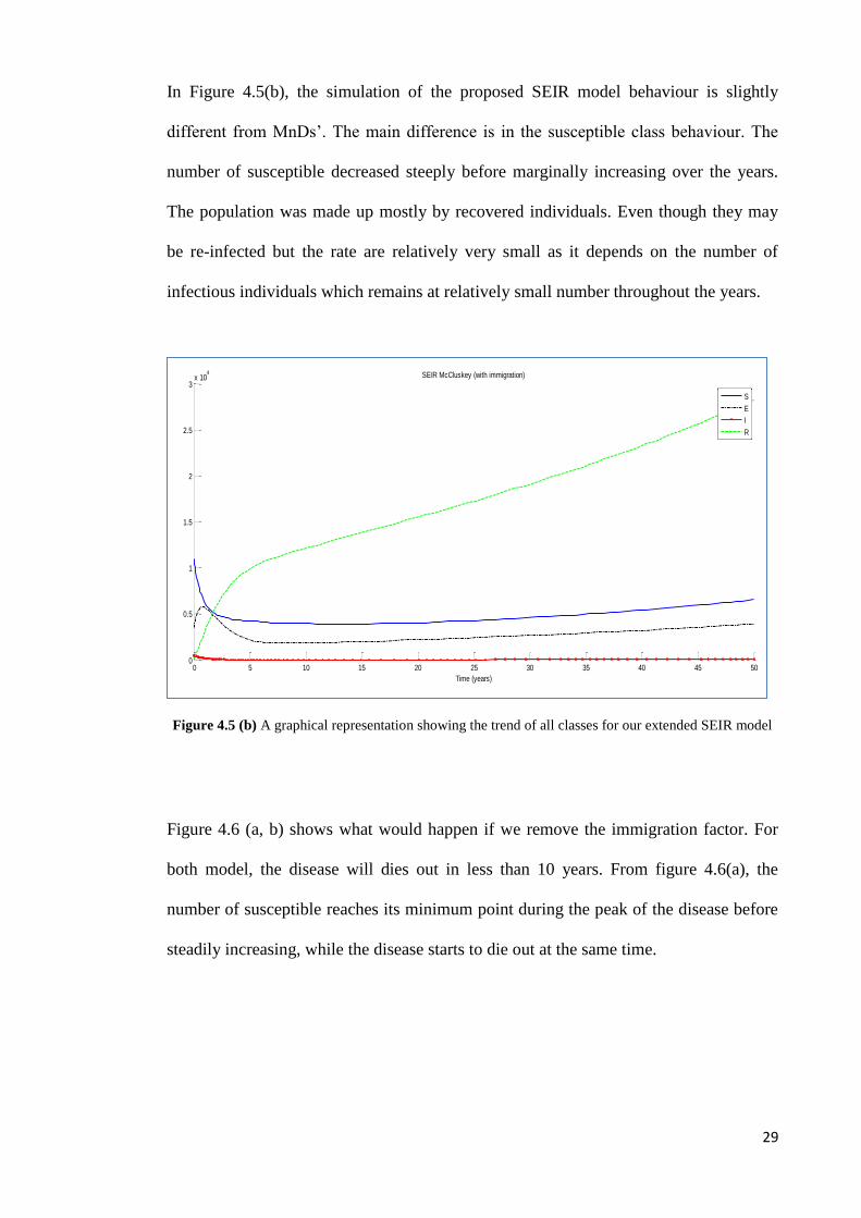
In Figure 4.5(b), the simulation of the proposed SEIR model behaviour is slightly

different from MnDs’. The main difference is in the susceptible class behaviour. The

number of susceptible decreased steeply before marginally increasing over the years.

The population was made up mostly by recovered individuals. Even though they may

be re-infected but the rate are relatively very small as it depends on the number of

infectious individuals which remains at relatively small number throughout the years.

Figure 4.5 (b) A graphical representation showing the trend of all classes for our extended SEIR model

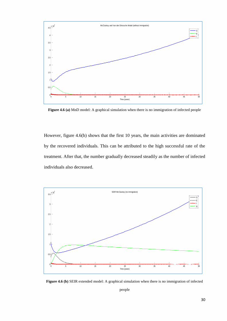
Figure 4.6 (a, b) shows what would happen if we remove the immigration factor. For

both model, the disease will dies out in less than 10 years. From figure 4.6(a), the

number of susceptible reaches its minimum point during the peak of the disease before

steadily increasing, while the disease starts to die out at the same time.

0 5 10 15 20 25 30 35 40 45 500

0.5

1

1.5

2

2.5

3x 10

4 SEIR McCluskey (with immigration)

Time (years)

S

E

I

R

30

Figure 4.6 (a) MnD model: A graphical simulation when there is no immigration of infected people

However, figure 4.6(b) shows that the first 10 years, the main activities are dominated

by the recovered individuals. This can be attributed to the high successful rate of the

treatment. After that, the number gradually decreased steadily as the number of infected

individuals also decreased.

Figure 4.6 (b) SEIR extended model: A graphical simulation when there is no immigration of infected

people

0 5 10 15 20 25 30 35 40 45 500

0.5

1

1.5

2

2.5

3

3.5

4

4.5x 10

4 McCluskey and Van den Driessche Model (without immigraiton)

Time (years)

S

E

I

0 5 10 15 20 25 30 35 40 45 500

0.5

1

1.5

2

2.5

3

3.5x 10

4 SEIR McCluskey (no immigration)

Time (years)

S

E

I

R

31

Figure 4.7 Effect of treatment

Figure 4.7 shows how important it is for the infected individuals to receive treatment. If

there is no treatment available, almost all the population will be latently infected by the

disease. Since the progression rate from latently infected to infectious are very low, the

number of infectious are kept at minimum. If given under some condition we cannot

treat all the infected people, a better option is to give treatment to those latently

infected individuals instead of the infectious ones.

Figure 4.8 (a) Treatment to the latently infected only

0 5 10 15 20 25 30 35 40 45 500

0.5

1

1.5

2

2.5

3

3.5x 10

4 SEIR McCluskey (without treatment)

Time (years)

S

E

I

R

0 5 10 15 20 25 30 35 40 45 500

0.5

1

1.5

2

2.5

3x 10

4 SEIR McCluskey (r1 = 0.7, r2 = 0)

Time (years)

S

E

I

R

32

Figure 4.8 (b) Treatment to the infectious only

As shown in Figure 4.8(a) above, treatment to the latently infected are more effective in

controlling the disease spreading compared to treatment given only to those infectious

(Figure 4.8(b)).

4.3.3. Conclusion

The model is a SEIR model based on the SEI tuberculosis model with immigration

proposed by McCluskey and P. van den Driessche [23]. We showed that both their

model and ours gave the same conclusion from the result. Here, the immigration of

infected individuals plays a very significant role that even with treatment the TB

remains endemic. However, even though there is a constant recruitment of infected

individuals into the population, the disease spreading can be kept at bay with successful

treatment. One of the effective ways to do so is by giving treatment to the latently

infected. On the other hand, when there is no immigration of infected, the disease will

dies out.

0 5 10 15 20 25 30 35 40 45 500

0.5

1

1.5

2

2.5

3

3.5x 10

4 SEIR McCluskey (r1 = 0.0, r2 = 0.55)

Time (years)

S

E

I

R

33

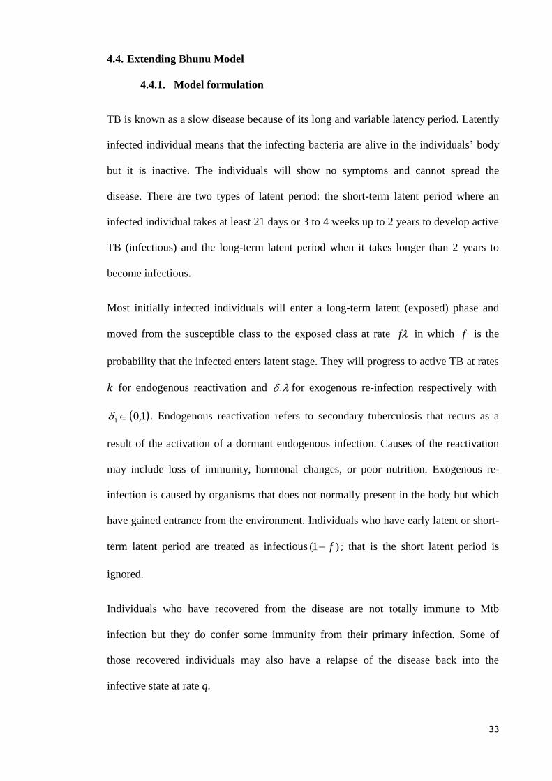
4.4. Extending Bhunu Model

4.4.1. Model formulation

TB is known as a slow disease because of its long and variable latency period. Latently

infected individual means that the infecting bacteria are alive in the individuals’ body

but it is inactive. The individuals will show no symptoms and cannot spread the

disease. There are two types of latent period: the short-term latent period where an

infected individual takes at least 21 days or 3 to 4 weeks up to 2 years to develop active

TB (infectious) and the long-term latent period when it takes longer than 2 years to

become infectious.

Most initially infected individuals will enter a long-term latent (exposed) phase and

moved from the susceptible class to the exposed class at rate f in which f is the

probability that the infected enters latent stage. They will progress to active TB at rates

for endogenous reactivation and 1for exogenous re-infection respectively with

1,01 . Endogenous reactivation refers to secondary tuberculosis that recurs as a

result of the activation of a dormant endogenous infection. Causes of the reactivation

may include loss of immunity, hormonal changes, or poor nutrition. Exogenous re-

infection is caused by organisms that does not normally present in the body but which

have gained entrance from the environment. Individuals who have early latent or short-

term latent period are treated as infectious )1( f ; that is the short latent period is

ignored.

Individuals who have recovered from the disease are not totally immune to Mtb

infection but they do confer some immunity from their primary infection. Some of

those recovered individuals may also have a relapse of the disease back into the

infective state at rate q.

34

These assumptions result in the following system of differential equations:

)18()(

)18()()1(

)18()(

)18()()1(

212

21

121

dIrErRqRpIdt

dR

cIrqRIpdkEESfNbdt

dI

bErREkESfNadt

dE

aSNbadt

dS

with initial condition

0)0(,0)0(,0)0( 000 IIEESS and )18(0)0( 0 eRR

Figure 4.9: Structure of model

Nba )1(

S

f

Na)1( f E

1 k

Nb

1r 2

dI

q2r p

R

35

The flow diagram of the disease is shown in Figure 4.9 above.

Based on the biological considerations, model system (18) will be studied in the region

,:,,, 4

NRIESRIESH

which is positively invariant with respect to system (18).

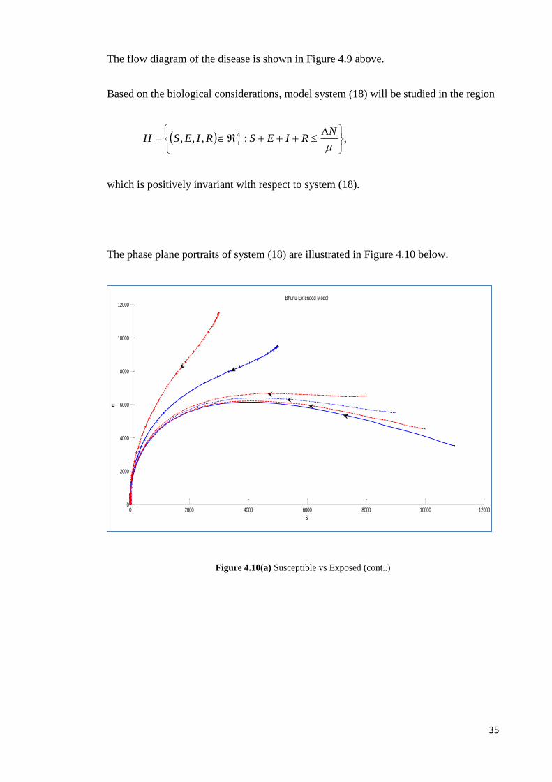
The phase plane portraits of system (18) are illustrated in Figure 4.10 below.

Figure 4.10(a) Susceptible vs Exposed (cont..)

0 2000 4000 6000 8000 10000 120000

2000

4000

6000

8000

10000

12000Bhunu Extended Model

S

E

36

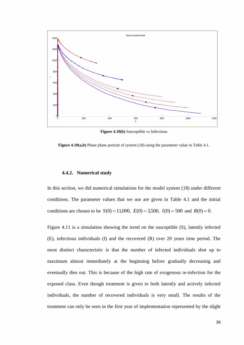
Figure 4.10(b) Susceptible vs Infectious

Figure 4.10(a,b) Phase plane portrait of system (18) using the parameter value in Table 4.1.

4.4.2. Numerical study

In this section, we did numerical simulations for the model system (18) under different

conditions. The parameter values that we use are given in Table 4.1 and the initial

conditions are chosen to be 500)0(,500,3)0(,000,11)0( IES and .0)0( R

Figure 4.11 is a simulation showing the trend on the susceptible (S), latently infected

(E), infectious individuals (I) and the recovered (R) over 20 years time period. The

most distinct characteristic is that the number of infected individuals shot up to

maximum almost immediately at the beginning before gradually decreasing and

eventually dies out. This is because of the high rate of exogenous re-infection for the

exposed class. Even though treatment is given to both latently and actively infected

individuals, the number of recovered individuals is very small. The results of the

treatment can only be seen in the first year of implementation represented by the slight

0 2000 4000 6000 8000 10000 120000

2000

4000

6000

8000

10000

12000

14000Bhunu Extended Model

S

I

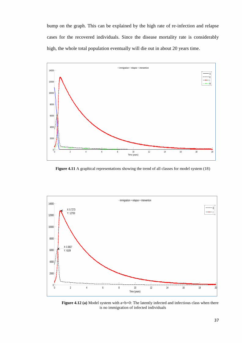
37

bump on the graph. This can be explained by the high rate of re-infection and relapse

cases for the recovered individuals. Since the disease mortality rate is considerably

high, the whole total population eventually will die out in about 20 years time.

Figure 4.11 A graphical representations showing the trend of all classes for model system (18)

Figure 4.12 (a) Model system with a=b=0: The latently infected and infectious class when there

is no immigration of infected individuals

0 2 4 6 8 10 12 14 16 18 200

2000

4000

6000

8000

10000

12000

14000+ immigration + relapse + intervention

Time (years)

S

E

I

R

0 2 4 6 8 10 12 14 16 18 200

2000

4000

6000

8000

10000

12000

14000- immigration + relapse + intervention

Time (years)

E

IX: 0.7273

Y: 12750

X: 0.3827

Y: 6109

38

Figure 4.12 (a, b) shows how immigration effects the TB transmission as a whole.

Figure 4.12(a) represents the latently and infectious class when there is no immigration

of infected individuals into the population. The peak for E class is 6,109 while the peak

for I class is 12,750.

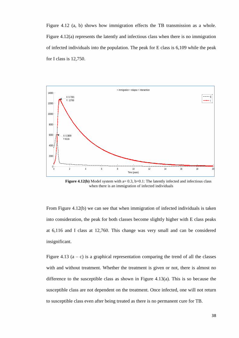
Figure 4.12(b) Model system with a= 0.3, b=0.1: The latently infected and infectious class

when there is an immigration of infected individuals

From Figure 4.12(b) we can see that when immigration of infected individuals is taken

into consideration, the peak for both classes become slightly higher with E class peaks

at 6,116 and I class at 12,760. This change was very small and can be considered

insignificant.

Figure 4.13 (a – c) is a graphical representation comparing the trend of all the classes

with and without treatment. Whether the treatment is given or not, there is almost no

difference to the susceptible class as shown in Figure 4.13(a). This is so because the

susceptible class are not dependent on the treatment. Once infected, one will not return

to susceptible class even after being treated as there is no permanent cure for TB.

0 2 4 6 8 10 12 14 16 18 200

2000

4000

6000

8000

10000

12000

14000+ immigration + relapse + intervention

Time (years)

E

I

X: 0.3809

Y:6116

X: 0.7301

Y: 12760

39

Figure 4.13 (a) The susceptible population with and without treatment

In Figure 4.13(b) we can see how the treatment affects both the latently infected

and infectious individuals. Even though there is not much of a difference, the treatment

clearly lowered the peak for both classes. Figure 4.13(c) shows a big difference to the

recovered population when treatment is given. The graph sky rocketed to its peak

before gradually decline as there is a decrease in the number of individuals in the

latently infected and infectious classes.

Figure 4.13 (b) The latently infected and the infectious population with and without treatment

0 1 2 3 4 5 6 7 8 9 100

2000

4000

6000

8000

10000

12000S with and without treatment

Time (years)

S with treatment

S without treatment

0 2 4 6 8 10 12 14 16 18 200

2000

4000

6000

8000

10000

12000

14000E - I with and without treatment

Time (years)

E with treatment

I with treatment

E without treatment

I without treatment

40

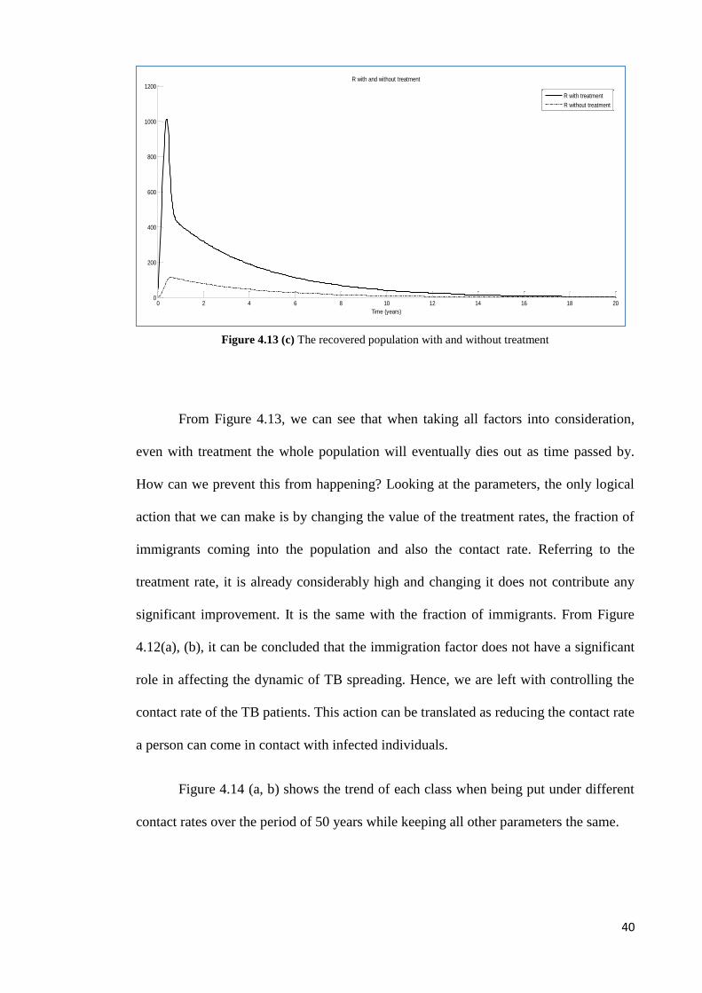
Figure 4.13 (c) The recovered population with and without treatment

From Figure 4.13, we can see that when taking all factors into consideration,

even with treatment the whole population will eventually dies out as time passed by.

How can we prevent this from happening? Looking at the parameters, the only logical

action that we can make is by changing the value of the treatment rates, the fraction of

immigrants coming into the population and also the contact rate. Referring to the

treatment rate, it is already considerably high and changing it does not contribute any

significant improvement. It is the same with the fraction of immigrants. From Figure

4.12(a), (b), it can be concluded that the immigration factor does not have a significant

role in affecting the dynamic of TB spreading. Hence, we are left with controlling the

contact rate of the TB patients. This action can be translated as reducing the contact rate

a person can come in contact with infected individuals.

Figure 4.14 (a, b) shows the trend of each class when being put under different

contact rates over the period of 50 years while keeping all other parameters the same.

0 2 4 6 8 10 12 14 16 18 200

200

400

600

800

1000

1200R with and without treatment

Time (years)

R with treatment

R without treatment

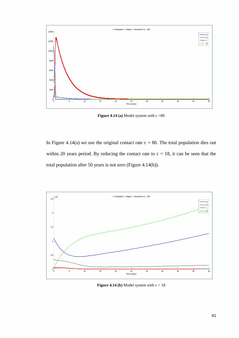
41

Figure 4.14 (a) Model system with c =80

In Figure 4.14(a) we use the original contact rate c = 80. The total population dies out

within 20 years period. By reducing the contact rate to c = 18, it can be seen that the

total population after 50 years is not zero (Figure 4.14(b)).

Figure 4.14 (b) Model system with c = 18

0 5 10 15 20 25 30 35 40 45 500

0.5

1

1.5

2

2.5x 10

4 + immigration + relapse + intervention (c = 18)

Time (years)

S

E

I

R

0 5 10 15 20 25 30 35 40 45 500

2000

4000

6000

8000

10000

12000

14000+ immigration + relapse + intervention (c = 80)

Time (years)

S

E

I

R

42

The number of recovered individuals keeps increasing over the years. Not only that, we

also manage to keep the number of infected at bay. This means that treatment with

quarantine proved to be the more efficient method in containing the disease as a whole.

Figure 4.15 shows that, with treatment, as long as we reduce the contact rate to less or

equal to 18, the total population will live on and we can successfully contained the

disease.

Figure 4.15 Total population with various contact rates, c.

4.4.3. Conclusion

The third model is the extended model where we incorporate the immigration factor

into the model proposed by Bhunu et al [5]. Even though in reality immigrants do play

a significant role in spreading the TB disease, the results that we obtained proved

otherwise. One reason is because since this model takes into consideration too many

factors into it, it overwhelms the immigration factor making it less significant. The

same thing can be said about the effectiveness of the treatment as a whole. Simply

giving the treatments is not the best option in a long term basis as the population will

0 5 10 15 20 25 30 35 40 45 500

0.5

1

1.5

2

2.5

3

3.5

4x 10

4 Total population, N with various c

Time (years)

Tota

l popula

tion,

N

c = 80

c = 19

c = 18

43

eventually dies out. Different kinds of intervention are needed to ensure a more

successful prevention plan. In this case, we showed that one way to do just that is by

reducing the contact rate of the infectious individuals.

44

CHAPTER 5

CONCLUSION AND FUTURE RESEARCH

5.1. Conclusion

Three mathematical models with immigration have been presented and studied to

analyze the dynamic of tuberculosis transmission under different conditions in order to

identify key factors which contribute in the spreading of the disease.

We started with a basic SEIR model [Equation 1(a – e), Figure 4.1] with the

assumption of permanent immunity and homogenous mixing. Using the model, we

analyze the local dynamics. A numerical solution presented in Figure 4.2 shows the

existence of a globally asymptotically stable endemic equilibrium under certain

parameter restrictions.

Next, we extended a SEI model [Figure 4.3(a)] of McCluskey and van den Driessche

[23] into a SEIR model [Equation 17 (a – e), Figure 4.3(b)]. In our model, instead of

the complete recovery that goes back to the susceptible population, the treated

individuals are moved into the recovered group. The results from both models are

compared, and we found that they basically give the same conclusion; that is,

immigration of infected individuals plays a very significant role in that the TB never

dies out [Figure 4.5]. However, the disease spreading can be kept at bay with effective

treatment. Our numerical result [Figure 4.8(a)] also shows that treatment to the latently

infected is more effective in keeping the disease under control.

We then incorporate the immigration factor to the model proposed by Bhunu et al [5] to

study the effects of immigration under different conditions. This model takes into

consideration the relapse, re-infection and re-activation of the disease. From this model

45

[Equation 18 (a – e)], we found out that the effect of immigration will be overwhelmed

by the other factors such as the high rate of re-infection [Figure 4.12]. Simply giving

treatments to the infected are definitely not enough since the population will eventually

dies out [Figure 4.11]. We showed that by reducing the contact rate of the infectious,

the spread of the disease can be controlled [Figure 4.14(b)].

From all the above results, we can conclude that immigration plays a significant role in

the dynamic of TB spreading since it has a marked influence to the existence of the

disease in the population [Figure 4.6]. However, its effect varies depending on other

contributing factors in the area involved. In order to control the spread of the disease, it

is very important for the TB patients to receive treatment [Figure 4.7 and 4.13].

Different kinds of intervention are needed to ensure a more successful prevention plan.

If the affected area has a low incidence rate, then with proper treatment, the spread of

the disease can still be controlled and the immigration of infected will not cause much

influence to the population [Figure 4.5(b)]. It is also better to give treatments to the

latently infected in order to avoid them becoming infectious and thus keeping the

incidence rate at a low level [Figure 4.8]. However, in the area where the prevalence

rate is high, the best action plan will be to give treatments to the infected and to

quarantine them so that their contact rate with others are reduces and thus lowering the

possibility of spreading the disease [Figure 4.14].

46

5.2. Recommendations for Future Research

We find out that the immigration factors that we used are not accurate enough to

represent the complexity of the real world. This may be due to the linear form chosen.

It might be a good idea to do a future research with a better approximation of

immigration factor using non-linear terms.

Furthermore, if we are to build a model that take into consideration intervention that

involves quarantine, it is better to do a sub-model instead of just one gross model to

differentiate the quarantine population and the normal population.

47

APPENDIXES

APPENDIX A

Compound Matrices

An mm matrix A with real entries will be identified with the linear operator on m

that it represents. Let "" denote the exterior product in m . With respect to the

canonical basis in the exterior product space m2 , the second additive compound

matrix ]2[A of A represents a linear operator on m2 whose definition on a

decomposable element 21 uu is

)()()( 212121

]2[ uAuuuAuuA

Definition over all of m2 is through linear extension. The entries in ]2[A are linear

relations of those in A. Let )( ijaA . For any integer

2,...,1

mi , let ),()( 21 iii be

the ith member in the lexicographic ordering of integer pairs such that mii 211 .

Then, the entry in the ith row and the jth column of ]2[AZ is

entriesmoreortwoinjfromdiffersiif

iinoccurnotdoesjandjinoccur

notdoesiofientryoneexactlyfa

jifaa

z r

s

ji

sr

iiii

ijrs

0

,)1(

)()(2211

For any integer mk 1 , the kth additive compound matrix ]2[A of A is defined

canonically. Pertinent to our purpose is a spectral property of ]2[A given in the

following proposition. Let }...,,1:{)( miA i be the spectrum of A.

48

Proposition. The spectrum of }.1:{)(, 2121

]2[]2[ miiAA ii

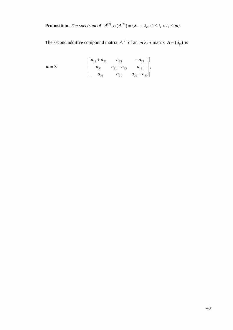
The second additive compound matrix ]2[A of an mm matrix )( ijaA is

,:3

33222131

12331132

13232211

aaaa

aaaa

aaaa

m

49

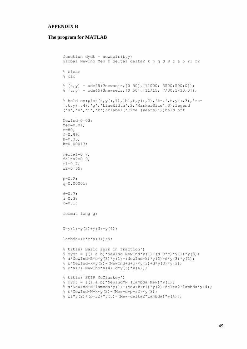
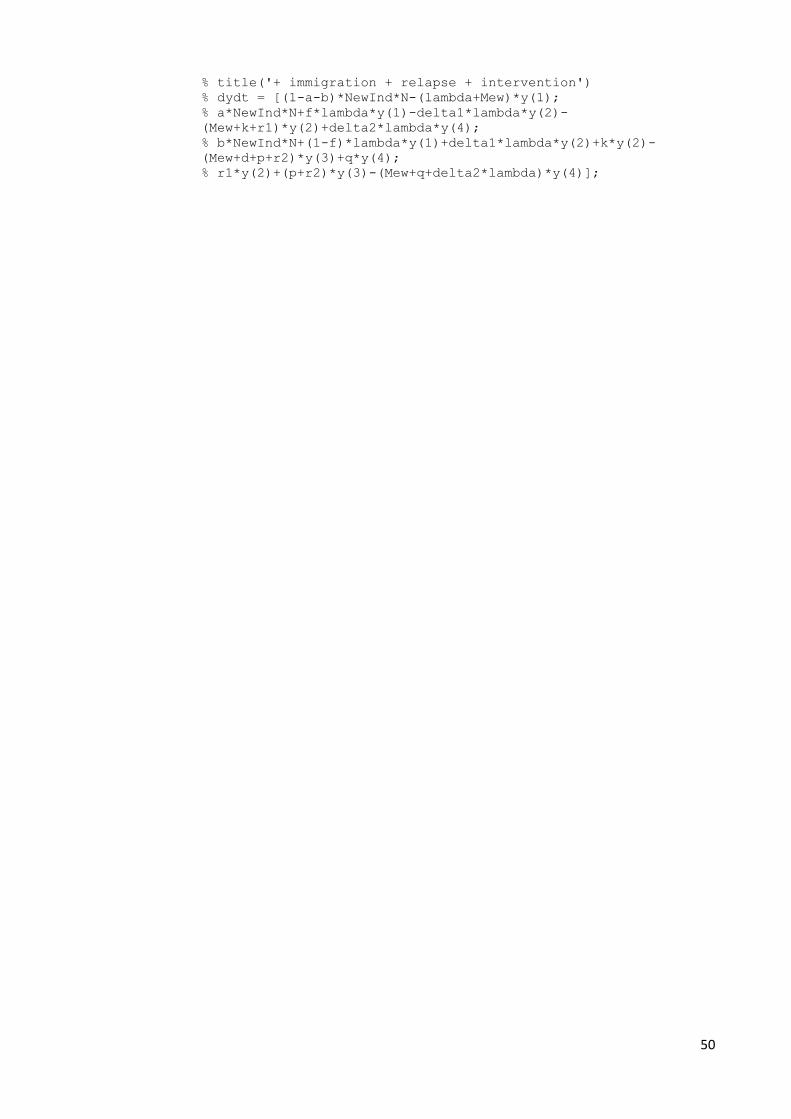
APPENDIX B

The program for MATLAB

function dydt = newseir(t,y) global NewInd Mew f delta1 delta2 k p q d B c a b r1 r2

% clear % clc

% [t,y] = ode45(@newseir,[0 50],[11000; 3500;500;0]); % [t,y] = ode45(@newseir,[0 50],[11/15; 7/30;1/30;0]);

% hold on;plot(t,y(:,1),'b',t,y(:,2),'k-.',t,y(:,3),'rx-

',t,y(:,4),'g','LineWidth',2,'MarkerSize',3);legend

('s','e','i','r');xlabel('Time (years)');hold off

NewInd=0.03; Mew=0.01; c=80; f=0.99; B=0.35; k=0.00013;

delta1=0.7; delta2=0.9; r1=0.7; r2=0.55;

p=0.2; q=0.00001;

d=0.3; a=0.3; b=0.1;

format long g;

N=y(1)+y(2)+y(3)+y(4);

lambda=(B*c*y(3))/N;

% title('Basic seir in fraction') % dydt = [(1-a-b)*NewInd-NewInd*y(1)+(d-B*c)*y(1)*y(3); % a*NewInd+B*c*y(3)*y(1)-(NewInd+k)*y(2)+d*y(3)*y(2); % b*NewInd+k*y(2)-(NewInd+d+p)*y(3)+d*y(3)*y(3); % p*y(3)-NewInd*y(4)+d*y(3)*y(4)];

% title('SEIR McCluskey') % dydt = [(1-a-b)*NewInd*N-(lambda+Mew)*y(1); % a*NewInd*N+lambda*y(1)-(Mew+k+r1)*y(2)+delta2*lambda*y(4); % b*NewInd*N+k*y(2)-(Mew+d+p+r2)*y(3); % r1*y(2)+(p+r2)*y(3)-(Mew+delta2*lambda)*y(4)];

50

% title('+ immigration + relapse + intervention') % dydt = [(1-a-b)*NewInd*N-(lambda+Mew)*y(1); % a*NewInd*N+f*lambda*y(1)-delta1*lambda*y(2)-

(Mew+k+r1)*y(2)+delta2*lambda*y(4); % b*NewInd*N+(1-f)*lambda*y(1)+delta1*lambda*y(2)+k*y(2)-

(Mew+d+p+r2)*y(3)+q*y(4); % r1*y(2)+(p+r2)*y(3)-(Mew+q+delta2*lambda)*y(4)];

51

BIBLIOGRAPHY

1. Anderson, R.M., & May R.M. (1991). Infectious Diseases of Humans.

Dynamics and Control. Oxford University Press, Oxford.

2. Aron, J.L. (2006). Mathematical Modeling: The Dynamics of Infection (Nelson,

K.E., & Williams, C.M., Eds.). In Infectious Disease Epidemiology: Theory

and Practice. (2nd

Ed., Chap. 6). Sudbury, MA: Jones & Bartlett Publishers.

3. Bailey, N.T.J. (1975). The Mathematical Theory of Infectious Disease, 2nd

ed.,

New York: Hafner

4. Bernoulli, D. (1769). Essai d'une nouvelle analyse de la mortalit6 causee par la

petite v6role et des avantages de l'inoculation pour la pr6venir, in Memoires de

Mathematiques et de Physique (pp. 1 45). Paris: Academie Royale des Sciences.

5. Bhunu, C.P., Garira, W., Mukandavire, Z., & Zimba, M. (2008). Tuberculosis

Transmission Model with Chemoprophylaxis and Treatment. Bulletin of

Mathematical Biology, 70, 1163-1191.

6. Brauer, F. & van den Driessche, P. (2001). Models for Transmission of Disease

with Immigration of Infectives. Mathematical Biosciences, 171, 143-154.

7. Choisy, M., Guégan, J.F., & Rohani, P., (2007). Mathematical modeling of

infectious diseases dynamics. In Tibayrene, M. (Ed.), Encyclopedia of

Infectious Diseases: Modern Methodologies (pp. 379–404).Hoboken: Wiley.

8. Dye, C., & Williams, B. G. (2000). Criteria for the control of drug-resistant

tuberculosis. Proceedings of the National Academy of Sciences, 97(14), 8180-

8185.

52

9. Dye, C., Scheele, S., Dolin, P., Pathania, V., & Raviglione, M. C. (1999). For

the WHO global surveillance and monitoring project. Global burden of

tuberculosis estimated incidence, prevalence and mortality by country. J. Am.

Med. Assoc. 282, 677–686.

10. Feldman, F. M. (1957). How Much Control of Tuberculosis 1937-1957-1977?

Am J Public Health Nations Health. October; 47(10), 1235–1241.

11. Fenner, L., Gagneux, S., Helbling, P., Battegay, M., Rieder, H.L., et al. (2012).

Mycobacterium tuberculosis transmission in a low-incidence country: Role of

immigration and HIV infection. J Clin Microbiol. February; 50(2), 388-395.

12. Frost, W. H. (1937). How Much Control of Tuberculosis? A.J.P.H. August;

27(8): 759–766.

13. Hamer, W.H. (1906). Epidemic disease in England. Lancet, 1, pp. 733-739.

14. Herzog, B., (1998). History of tuberculosis. Respiration, 65 (1), 5-15.

15. Hethcote, H.W (2000). The Mathematics of Infectious Disease. SIAM REVIEW,

42(4), 599-653.

16. Jia Z.W, Tang G.Y, Zhen Jin, Dye C., Vlas S.J, Li X.W., et al (2008). Modeling

the Impact of Immigration on the Epidemiology of Tuberculosis. Theoretical

Population Biology, 73, 437–448.

17. Kamper-Jorgensen, Z., Andersen, A.B., Kok-Jensen, A., et al. (2012). Migrant

tuberculosis: the extent of transmission in a low burden country. BMC

Infectious Disease, Vol. 12:60.

18. Kermack, W.O., & McKendrick, A.G. (1927). A contribution to the

mathematical theory of epidemics. Proc R Soc Lond; A115:700–21.

19. Li, M.Y. & Muldowney, J.S. (1995). Global Stability for the SEIR Model in

Epidemiology. Mathematical Biosciences, 125, 155-164.

53

20. Li, M.Y., Graef, J.R., Wang & L., Karsai, J. (1999). Global Dynamics of A

SEIR Model with Varying Total Population Size. Mathematical Biosciences,

160, 191-213.

21. Liu, W-M., Hethcote, H.W. & Levin, S.A. (1987). ‘ynamical behavior of

epidemiological models with nonlinear incidence rates’ J. Math. Biol, 25: 359-

380.

22. Lillebaek, T., Andersen, A.B., Dirksen, A., Smith, E., Skovgaard, L.T., & Kok-

Jensen, A. (2002). Persistent high incidence of tuberculosis in immigrants in a

low-incidence country. Emerg. Infect. Diseases 8, 679–684.

23. McCluskey, C.C. & van den Driessche, P. (2004). Global Analysis of Two

Tuberculosis Models. Journal of Dynamics and Differential Equations, Vol.16,

139-166.

24. Ross R. The Prevention of Malaria. Murray, London, 1911.

25. Schoenstadt, A., (August 26, 2008). Tuberculosis. Retrieved 24 February 2012

from http://tuberculosis.emedtv.com/tuberculosis/tuberculosis.html

26. Song, B., Castillo-Chavez, C., & Aparicio, J.P. (2002). Tuberculosis models

with fast and slow dynamics: the role of close and casual contacts. Math. Biosci.

180, 29-48.

27. Waaler, H., Geser, A., & Andersen, S. The Use of Mathematical Models in the

Study of the Epidemiology of Tuberculosis. American Journal of Public Health

and the Nations Health, June 1962; 52(6), 1002-1013.

28. World Health Organization (November 2010). Tuberculosis Fact sheet N°104.

Retrieved 25 August 2011 from

http://www.who.int/mediacentre/factsheets/fs104/en/index.html