8/4/2019 N-Body Self Gravity

http://slidepdf.com/reader/full/n-body-self-gravity 1/11

The Astrophysical Journal, 703:1363–1373, 2009 October 1 doi:10.1088/0004-637X/703/2/1363

C 2009. The American Astronomical Society. All rights reserved. Printed in the U.S.A.

 N -BODY SIMULATION OF PLANETESIMAL FORMATION THROUGH GRAVITATIONAL INSTABILITY ANDCOAGULATION. II. ACCRETION MODEL

Shugo Michikoshi1, Eiichiro Kokubo1,2, and Shu-ichiro Inutsuka3

1 Center for Computational Astrophysics, National Astronomical Observatory of Japan, Osawa, Mitaka, Tokyo 181-8588, Japan; michikoshi@cfca.jp,kokubo@th.nao.ac.jp

2 Division of Theoretical Astronomy, National Astronomical Observatory of Japan, Osawa, Mitaka, Tokyo 181-8588, Japan3

Department of Physics, Kyoto University, Kyoto 606-8502, Japan; inutsuka@tap.scphys.kyoto-u.ac.jp Received 2008 December 19; accepted 2009 August 12; published 2009 September 9

ABSTRACT

The gravitational instability of a dust layer is one of the scenarios for planetesimal formation. If the density of a dust layer becomes sufficiently high as a result of the sedimentation of dust grains toward the midplane of aprotoplanetary disk, the layer becomes gravitationally unstable and spontaneously fragments into planetesimals.Using a shearing box method, we performed local N -body simulations of gravitational instability of a dustlayer and subsequent coagulation without gas and investigated the basic formation process of planetesimals.In this paper, we adopted the accretion model as a collision model. A gravitationally bound pair of particlesis replaced by a single particle with the total mass of the pair. This accretion model enables us to performlong-term and large-scale calculations. We confirmed that the formation process of planetesimals is the sameas that in the previous paper with the rubble pile models. The formation process is divided into three stages:the formation of nonaxisymmetric structures; the creation of planetesimal seeds; and their collisional growth.

We investigated the dependence of the planetesimal mass on the simulation domain size. We found thatthe mean mass of planetesimals formed in simulations is proportional to L

3/2y , where L y is the size of the

computational domain in the direction of rotation. However, the mean mass of planetesimals is independentof  L x, where L x is the size of the computational domain in the radial direction if  L x is sufficiently large. Wepresented the estimation formula of the planetesimal mass taking into account the simulation domain size.

Key words: gravitation – instabilities – methods: N -body simulations – planets and satellites: formation

1. INTRODUCTION

According to the standard theory of planet formation, plan-ets form from planetesimals, which are kilometer-sized solidbodies. However, the process of planetesimal formation is still

controversial. The inward migration of meter-sized bodies dueto gas drag is very rapid; its timescale is only 102 yr (Adachiet al. 1976; Weidenschilling 1977). The growth of dust to plan-etesimals due to particle adhering seems difficult in the standarddisk model.

The gravitational instability scenario is an alternative sce-nario for this stage (Safronov 1969; Goldreich & Ward 1973).Dust particles settle into the midplane of a protoplanetarydisk owing to the gravitational force from the central star if the gas flow is laminar. As the sedimentation of dust parti-cles proceeds, the density at the midplane exceeds the crit-ical density, and the dust layer finally becomes gravitation-ally unstable. The gravitationally unstable dust layer rapidlycollapses by its self-gravity, forming km-sized planetesimals

(Goldreich & Ward 1973; Coradini et al. 1981; Sekiya 1983).The rapid migration of meter-sized bodies can be avoided be-cause the timescale of the gravitational instability is only onthe order of a Kepler period. However, the gravitational insta-bility scenario has a critical issue. As the sedimentation of dustgrains toward the midplane proceeds, the vertical velocity shearincreases and gives rise to the Kelvin–Helmholtz instability,which makes the dust layer turbulent. The turbulence preventsdust particles from settling. A lot of studies have been car-ried out on this issue (Weidenschilling 1980; Cuzzi et al. 1993;Champney et al. 1995; Weidenschilling 1995; Sekiya 1998;Dobrovolskis et al. 1999; Sekiya & Ishitsu 2000, 2001; Ishitsu& Sekiya 2002, 2003; Michikoshi & Inutsuka 2006). However,

problems concerning the gravitational instability still remainunsettled.

Although many studies have been conducted on the conditionof gravitational instability or its linear regime, there has beenlittle study of the nonlinear regime of gravitational instability.

Here we concentrate on the formation process of planetesimalsassuming the gravitational instability. Tanga et al. (2004) per-formed N -body simulations of a gravitationally unstable particledisk. In their simulation, the optical depth is very small, andthe particle disk is unstable, even initially. If we consider theformation of planetesimals through gravitational instability ata0 1 AU, the optical depth is high, and the initial velocitydispersion must be large owing to turbulent flow driven by theKelvin–Helmholtz instability or magnetorotational instability(Balbus & Hawley 1991). In our analysis, we will take a closelook at initially stable disks with large optical depth. Johansenet al. (2007) performed simulations using a code that solvesthe magnetohydrodynamic equations with a three-dimensionalgrid and includes particles with self-gravity. They mapped the

particle density on the grid and solved the Poisson equation us-ing a fast Fourier transform method. They included collisionsamong particles as damping the velocity dispersion of the par-ticles within each grid. They found that particles collapse in anoverdense region in the midplane and the gravitationally boundobjects form with masses comparable to dwarf planets.

Michikoshi et al. (2007) performed a set of simulations inthe self-gravitating collision-dominated particle disks withoutgas components (hereafter Paper I). The point-to-point Newto-nian mutual interaction was calculated directly. They adoptedthe hard and soft sphere models as collision models, and ex-amined parameter dependencies on the size of computationaldomain, restitution coefficient, optical depth, Hill radius of 

1363

8/4/2019 N-Body Self Gravity

http://slidepdf.com/reader/full/n-body-self-gravity 2/11

1364 MICHIKOSHI, KOKUBO, & INUTSUKA Vol. 703

particles, and the duration of collision. In the hard sphere model,penetration between particles is not possible (e.g., Wisdom &Tremaine 1988; Salo 1991; Richardson 1994; Daisaka & Ida1999; Daisaka et al. 2001). The velocity changes in an instantat collisions. In the soft sphere model, particles can overlap if they are in contact (e.g., Salo 1995). They found that the for-mation process of planetesimals is qualitatively independent of simulation parameters if initial Toomre’s Q value, Qinit > 2.The formation process is divided into three stages: the forma-tion of nonaxisymmetric wake-like structures (Salo 1995), thecreation of aggregates, and the rapid collisional growth of theaggregates. The mass of the largest aggregates is larger thanthe mass predicted by the linear perturbation theory (here-after linear mass M linear; Goldreich & Ward 1973). HoweverMichikoshi et al. (2007) could not find the saturation of thegrowth of the planetesimals in Paper I. The mass of the planetes-imal formed in the simulation depends on the size of the compu-tational domain. Almost allmass in the computational domain isabsorbed by a single planetesimal, and thus the mass of the plan-etesimal is determined by the total mass in the computationaldomain.

In this paper, we use the alternative model of collisions,

“accretion model.” In physical terms, the accretion modelcorresponds to the more dissipative model than the hard andsoft sphere models. In the accretion model, when two particlescollide, if the binding condition is satisfied, the two particlesare merged into one particle. Efficient energy dissipation occurswhen two particles merge into one particle. In the soft andhard sphere models, since large aggregates consist of a lot of small particles and the number of particles does not decrease,the calculation is time-consuming. If we are not interested ininternal states of planetesimals such as rotation or internaldensity profile, we can treat a large aggregate as one largeparticle. We expect that the final mass or spatial distributionof planetesimals can be estimated by the accretion model.The accretion model has an advantage from the viewpoint of 

calculation. The number of particles decreases as the calculationproceeds; thereby this model enables us to perform simulationsof larger numbers of particles than that in the previous work.Taking this advantage, we can examine the large computationaldomains.

In this study, we neglect the effect of gas for the sakeof simplicity. As many authors investigated, the effect of gas is very important. The solid particles drift radially dueto gas drag (Adachi et al. 1976; Weidenschilling 1977), gasfriction helps gravitational collapse (Ward 1976; Youdin 2005a,2005b), gas turbulence prevents and helps concentration of solids (Weidenschilling & Cuzzi 1993; Barge & Sommeria1995; Fromang & Nelson 2006; Johansen et al. 2006a), andclumps of solid particles form due to streaming instability

(Youdin & Goodman 2005; Johansen et al. 2006b; Johansenet al. 2007). But once gravitational instability happens and largeaggregates form, as a first step, we may be able to neglectgas drag because they are so large that they decouple fromgas. Therefore our gas-free model may be applicable to thestages of gravitational instability and subsequent collisionalgrowth.

In Section 2, we explain the simulation method. Our resultsare presented in Section 3. We compare the accretion modelwith the soft and hard sphere models and investigate the modelsof large computational domain. In Section 4, we summarize theresults.

2. METHODS OF CALCULATION

The method of calculation is the same as that used in Paper Iexcept for the collision model, which is based on the method of simulation of planetary rings (e.g., Wisdom & Tremaine 1988;Salo 1991; Daisaka & Ida 1999; Ohtsuki & Emori 2000).

We introduce rotating Cartesian coordinates (x , y , z) calledHill coordinates, the x-axis pointing radially outward, the y-axispointing in the direction of rotation, and the z-axis normal to

the equatorial plane. The origin of the coordinates moves on acircular orbit with the semimajor axis a0 and the Keplerianangular velocity Ω0. Assuming |xj |, |yj |, |zj | a0, where(xj , yj , zj ) is the position of  jth particle, we can write theequation of motion in nondimensional forms independent of the

mass and the semimajor axis a0, if we scale the time by Ω−10 ,

the length by Hill radius ha0, and the mass by h3M ∗, whereh = (2mp/3M ∗)1/3, mp is the characteristic mass of particles,and M ∗ is the mass of the central star (e.g., Petit & Henon 1986;Nakazawa & Ida 1988):

d 2xi

d t 2= 2

d yi

d t + 3xi +

N 

j

=1,j

=i

mj

˜r 3

ij

(xj − xi ),

d 2yi

d t 2= −2

d xi

d t +

N j=1,j=i

mj

r3ij

(yj − yi ),

d 2zi

d t 2= −zi +

N j=1,j=i

mj

r3ij

(yj − yi ),

(1)

where a tilde denotes corresponding nondimensional variables,rij is the distance between particles i and j, and N is the numberof particles.

We use the periodic boundary condition (Wisdom & Tremaine1988). There are an active region and its copies. Inner andouter regions have different angular velocities. These regionsslide upward and downward with shear velocity 3Ω0Lx /2,

where L x is the length of the cell in the x-direction. We calculategravitational forces from particles in these regions. We use thespecial-purpose computer GRAPE-6 for the calculation of self-gravity (Makino et al. 2003).

Particles used in the simulation are not realistic dust particlesbut superparticles that represent a group of small particles; thus,the parameter used in this paper is not exactly the physicalrestitution coefficient but corresponds to the coefficient of thedissipation due to collisions among particles. The collisionmodels used in Paper I cannot treat more dissipative modelswhere the tangential coefficients of restitution t < 1 becausewe adopt t = 1. The net restitution coefficient is =

2

n v2

n + 2

t v2

t v2

n +

v2

t , where n is the normal coefficient

of restitution, vn and vt are normal and tangential velocities

of a collision (Canup & Esposito 1995). The net restitutioncoefficient is always larger than 0.7 if we assume t = 1 andv2

n

= v2

t

. If we allow t = 1 in order to examine the model of 

< 0.7, we must consider rotations of individual particles. Forthe sake of simplicity, we ignore rotations of particles in thispaper and assume t = 1.

The way to treat a collision is to use the same method appliedto the hard sphere model, but we consider the binding conditionof colliding particles. If a pair overlaps, rij < rp,i + rp,j , whererp,i is a radius of particle i, and is approaching, nij · vij < 0,where vij is the relative velocity and nij is a unit vector along

8/4/2019 N-Body Self Gravity

http://slidepdf.com/reader/full/n-body-self-gravity 3/11

No. 2, 2009 FORMATION OF PLANETESIMALS. II. 1365

rij = (xj , yj , zj )− (xi , yi , zi ), we assume that this pair collides,and changes its velocities by using the equations of collision:

vi = vi − mj

mi + mj

(1 + )(nij · vij )nij , (2)

vj = vj +

mi

mi + mj

(1 + )(nij · vij )nij , (3)

where is a restitution coefficient. Using the updated velocities,we check whether thebinding conditionis satisfied by theJacobiintegral (e.g., Nakazawa & Ida 1988):

J ij = 1

2

˙xij

2+ ˙yij

2+ ˙zij

2− 3

2x2

ij +1

2z2

ij − 3

rij

+9

2< 0, (4)

where ( ˙xij , ˙yij , ˙zij ) is the relative velocity. If the pair is bound,two particles are merged into one particle conserving theirmomentum. The shape of the new particle is a sphere, the radiusof which is determined by its mass.

We assume that all particles have the same mass mp initially.The parameters of the present simulation are the distance fromthe central star a0, the length of region L x and L y, the number of 

particles N , and the mass of particles mp(rp, ρp), where ρp is thedensity of a particle. The dynamical behavior is characterizedby only two nondimensional parameters (Daisaka & Ida 1999);the initial optical depth τ  and the ratio ζ = a0h/2rp. In themodels of  ζ > 1, the centers of the particles are in their Hillsphere when two particles come into contact. The initial opticaldepth is given by Goldreich & Tremaine (e.g., 1982)

τ  = 3Σ

4ρprp

= 0.19

Σ

10 g cm−2

ρp

2 g cm−3

−1

× rp

20 cm

−1

, (5)

where Σ is the surface density of particles. The ratio ζ is givenby

ζ = 105.528

M M ∗

−1/3 ρp

2 g cm−3

1/3 a0

1 AU

. (6)

Using the above two parameters, the other parameters canbe estimated. The normalized most unstable wavelength of gravitational instability is (e.g., Sekiya 1983)

λmost = 12π τ ζ 2. (7)

The normalized size of computational domain L, the number of particles N , the normalized radius of particle

˜rp, and Toomre’s

Q value are given by

Lx = 12π Ax τ ζ 2, (8)

Ly = 12π Ay τ ζ 2, (9)

N  = 576π Ax Ay τ 3ζ 6, (10)

rp = 1

2ζ, (11)

Q = σ x

6τ ζ 2, (12)

Table 1

Initial Conditions and Results

Model τ ζ A x A y Qinit σ x M pl/M linear N pl

01 0.01 0.1 2.0 6.0 6.0 3.0 7.2 21.2 2

02 0.01 0.11 2.0 6.0 6.0 3.0 7.9 42.4 1

03 0.01 0.125 2.0 6.0 6.0 3.0 9.0 21.5 2

04 0.1 0.1 2.0 6.0 6.0 3.0 7.2 42.7 1

05 0.3 0.1 2.0 6.0 6.0 3.0 7.2 43.2 1

06 0.5 0.1 2.0 6.0 6.0 3.0 7.2 38.4 1

07 0.7 0.1 2.0 6.0 6.0 3.0 7.2 0.0 0

08 0.9 0.1 2.0 6.0 6.0 3.0 7.2 0.0 0

09 0.01 0.06 2.5 6.0 6.0 3.0 6.8 43.4 1

10 0.01 0.06 2.7 6.0 6.0 3.0 8.2 43.4 1

11 0.01 0.06 3.0 6.0 6.0 3.0 9.7 39.8 1

12 0.01 0.1 2.0 4.0 4.0 3.0 7.2 19.5 1

13 0.01 0.1 2.0 8.0 8.0 3.0 7.2 38.4 2

14 0.01 0.1 2.0 3.0 3.0 3.0 7.2 11.1 1

15 0.01 0.1 2.0 6.0 3.0 3.0 7.2 21.7 1

16 0.01 0.1 2.0 9.0 3.0 3.0 7.2 16.4 2

17 0.01 0.1 2.0 12.0 3.0 3.0 7.2 11.0 4

18 0.01 0.1 2.0 24.0 3.0 3.0 7.2 10.1 9

19 0.01 0.1 2.0 3.0 6.0 3.0 7.2 21.8 1

20 0.01 0.1 2.0 3.0 9.0 3.0 7.2 32.2 1

21 0.01 0.1 2.0 3.0 12.0 3.0 7.2 43.1 1

22 0.01 0.1 2.0 3.0 24.0 3.0 7.2 85.5 123 0.01 0.1 2.0 6.0 6.0 4.0 9.6 43.3 1

24 0.01 0.1 2.0 6.0 6.0 5.0 12.0 21.6 2

Notes. M pl, M linear and N pl are the mean planetesimal mass, the linear mass

and the number of planetesimals at final state, respectively.

where A x is the ratio Lx /λmost, A y is the ratio Ly /λmost, and σ xis the radial velocity dispersion scaled by a0hΩ0, respectively.In order to determine the size of the computational domain, weneed to set A x and A y. The initial velocity dispersion is also aparameter. We determine it from the initial Toomre’s Qinit valueusing Equation (12). As shown above, if we set τ , ζ , A x, A y,

and Qinit, we can determine the initial state. The simulationparameters are summarized in Table 1. We call model 1 as thestandard model. The number of particles is 1000–10,000.

If  ζ > 1.5, two particles can be bound (Ohtsuki 1993; Salo1995), so we need to adopt ζ > 1.5 in order to investigatethe formation process of planetesimals. In this paper, weuse ζ = 2, which is much smaller than the realistic valueζ 100. Thus the physical size of a particle in our simulationis very large. It indicates that the effect of the self-gravity isrelatively weaker than that of inelastic collisions. To investigategravitational instability, the particle density should be higherthan the Roche density. The particle density is ρp = 4ζ 3ρR,

where ρR = (9/4π)M ∗/a30 is the Roche density. Thus when

ζ

=2, ρp

ρR. So we can study gravitational instability

with this parameter. But this approximation may change theresult when comparing between ζ = 2 and ζ = 100, althoughgravitational instability occurs in both models. In the futurework, we will perform the simulation with a larger ζ value byusing next-generation supercomputers.

In most of the models, we set Qinit = 3, which corresponds toσ x 7.2 for the standard model. The characteristic velocity of the actual turbulence vturb is about ηvK, where vK is the Keplervelocity, η = −12

c2

s

v2

K

(∂ log P /∂ log r), cs is the sound

velocity of gas, P is the pressure of gas, and r  is the distancefrom the central star (Adachi et al. 1976; Weidenschilling 1977).At r = 1 AU, in the Hill unit, the characteristic velocity of theturbulence is vturb 1.3×107 that is much larger than σ x . If the

8/4/2019 N-Body Self Gravity

http://slidepdf.com/reader/full/n-body-self-gravity 4/11

1366 MICHIKOSHI, KOKUBO, & INUTSUKA Vol. 703

Figure 1. Spatial distribution of particles in the standard model (model 1) at t/ T K = 0.0 (top left panel), t/ T K = 0.4 (top middle panel), t/ T K = 0.8 (top right panel),t/ T K = 1.2 (bottom left panel), t/ T K = 1.6 (bottom middle panel), and t/ T K = 2.0 (bottom right panel). Circles represent particles and their size is proportional tothe physical size of particles.

turbulence weakens, Q decreases gradually from Q 1, andgravitational instability occurs finally. Therefore, we choose theinitial condition that the disk is gravitationally stable (Qinit = 3).

We set the initial velocities and positions of particles usingthe above parameters. A Keplerian orbit has six parameters: theposition of the guiding center (xg, yg), eccentricity e, inclination

i, and the two phases of epicycle and vertical motions (e.g.,Nakazawa & Ida 1988). The eccentricity e and inclination i of particles are assumed to obey the Rayleigh distribution with the

ratio

e2/i2 = 2 (Ida & Makino 1992). We set the positionof the guiding center and the two phases uniformly, avoidingoverlapping.

The equation of motion is integrated with a second-orderleapfrog scheme. We adopt the variable time step used byDaisaka & Ida (1999). The time step formula is given byΔt  = η mini |ai|/|ai|, where ai and ai are the acceleration of particle i and its time derivative, and η is a nondimensional timestep coefficient, respectively.

3. RESULTS

3.1. Time Evolution

Figure 1 shows snapshots in model 1 at t/T K =0.0, 0.4, 0.8, 1.2, 1.6, and 2.0 where T K is the orbital period2π/Ω0. At t/T K

=0.4, we cannot see any spatial structures

and large bodies. The formation process of planetesimals is thesame as those of the hard and soft sphere models (Paper I). Thenonaxisymmetric wake-like structure forms at t/T K = 0.8, 1.2,which appears if we consider self-gravity. The nonaxisymmet-ric wake-like structure is also seen in planetary rings (Salo1995). The density in the wake-like structure is higher than themean surface density Σ. For example, the surface density in thedense region is 1.52Σ at t/T K = 1.6. Planetesimal seeds formin the dense parts of these wakes by fragmentation (t/T K =1.6, 2.0). Here we consider the formation of the wake-likestructure and planetesimal seeds as the gravitational instabilitystage.

8/4/2019 N-Body Self Gravity

http://slidepdf.com/reader/full/n-body-self-gravity 5/11

No. 2, 2009 FORMATION OF PLANETESIMALS. II. 1367

Figure 2. Same as Figure 1 at t/ T K = 2.0 (top left panel), t/ T K = 3.0 (top middle panel), t/ T K = 4.0 (top right panel), t/ T K = 5.0 (bottom left panel), t/ T K = 6.0(bottom middle panel), and t/ T K = 7.0 (bottom right panel).

Figure 2 shows snapshots in model 1 at t/T K =2.0, 3.0, 4.0, 5.0, 6.0, and 7.0. Once planetesimal seeds form,the nonaxisymmetric wake-like structures disappears (t/T K =3.0). Planetesimal seeds grow rapidly by mutual coalescence(t/T K = 3.0, 4.0, 5.0). In this stage, the disk is gravitationallystable. The gravitation seems to merely enhance the coalescentgrowth. When almost all planetesimal seeds are absorbed by a

few planetesimals, the growth slows down (t/T K = 6.0, 7.0).This stage is the collisional growth stage.

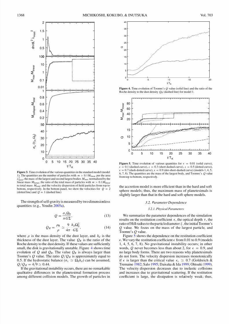
Figure 3 shows the time evolution of the number of largeparticles, the mass of the largest and second largest particles,the ratio of the mass of large particles to the total mass, andthe velocity dispersion of field particles for model 1. The timeevolution of the number of large particles is similar to thoseof the hard and soft sphere models (Paper I). The number of large particles has a maximum at t/T K 1.7, and its value isabout 1.2, which is slightly larger than that in the hard andsoft sphere models. However, the number of large particlesdecreases rapidly after t/T K 1.7. This decay is caused bythe fast coalescence of large particles.

The mass of the largest particle monotonically increasesup to about 44 M linear, which is twice larger than that of thehard and soft sphere models, where M linear = πΣ(λmost/2)2

is the planetesimal mass estimated by the linear theory.In the accretion model, the growth of planetesimals is en-hanced because sticking of dust grains is efficient. Themass of the second largest particle changes discontinuously,

when the second largest particle is absorbed by the largestone.

The ratio of the mass of the large particles to the total mass isalmost the same as that of the hard and soft sphere models. Theratio monotonically increasesup to about 1, andmost of themassin the computational domain is finally absorbed by the largeplanetesimals.

The velocity dispersion decreases until t/T K 1.3 becauseof the dissipation due to inelastic collisions. When the velocitydispersion becomes sufficiently small (Q 2), the gravitationalinstability occurs and a lot of planetesimal seeds form. Asthe field particles are scattered by the planetesimal seeds, thevelocity dispersion increases.

8/4/2019 N-Body Self Gravity

http://slidepdf.com/reader/full/n-body-self-gravity 6/11

1368 MICHIKOSHI, KOKUBO, & INUTSUKA Vol. 703

0

10

20

30

40

50

0 5 10 15 20 25 30 35 40

    σ  x

   /   (  r   H

     Ω   0   )

t/ TK

0

0.2

0.4

0.6

0.8

1

   M  c  o

   l   l  a  p  s  e

   /   M   t  o   t  a   l

0.01

0.1

1

10

100

   M  m  a  x

   /   M   l   i  n  e  a  r

0

0.5

1

1.5

2

   d  n   /   d   L   2      λ  m  o  s   t   2

Figure 3. Time evolution of the various quantities in the standard model (model1). The quantities are the number of particles with m > 0.1M linear per the areaλ2

most , the mass of the largest and second largest bodies M max normalized by thelinear mass M lienar, the ratio of the total mass of particles with m > 0.1M linear

to total mass M total and the velocity dispersion of field particles from top tobottom, respectively. In the bottom panel, we show the velocities for Q = 2(dotted line) and Q = 1 (dashed line)

The strength of self-gravity is measured by two dimensionlessquantities: (e.g., Youdin 2005a),

Q = σ xΩ0

π GΣ, (13)

QR =ρR

ρ 9

4π

hd Ω2

0GΣ , (14)

where ρ is the mass density of the dust layer, and hd  is thethickness of the dust layer. The value Q R is the ratio of theRoche density to the dust density. If these values are sufficientlysmall, the disk is gravitationally unstable. Figure 4 shows timeevolution of  Q and Q R. The value Q R is always larger thanToomre’s Q value. The ratio Q/QR is approximately equal to0.5. If the hydrostatic balance (σ x Ω0hd ) can be assumed,Q/QR = 4/9 0.44.

If the gravitational instability occurs, there are no remarkablequalitative differences in the planetesimal formation processamong different collision models. The growth of particles in

0

5

10

15

20

25

30

35

40

0 5 10 15 20

   Q

t/TK

Figure 4. Time evolution of Toomre’s Q value (solid line) and the ratio of theRoche density to the dust density Q R (dashed line) for model 1.

0

5

10

15

0 5 10 15 20 25 30 35 40

   Q

t/ TK

20

40

60

80

   M  m  a  x

   /   M   l   i  n  e  a  r

Figure 5. Time evolution of various quantities for = 0.01 (solid curve),

=0.1 (dashed curve),

=0.3 (short dashed curve),

=0.5 (dotted curve),

= 0.7 (dash-dotted curve), = 0.9 (dot-short-dashed curve) (models 1, 4, 5,6, 7, 8). The quantities are the mass of the largest body, and Toomre’s Q valuefrom top to bottom, respectively.

the accretion model is more efficient than in the hard and softsphere models; thus, the maximum mass of planetesimals isslightly larger than that in the hard and soft sphere models.

3.2. Parameter Dependence

3.2.1. Physical Parameters

We summarize the parameter dependences of the simulationresults on the restitution coefficient , the optical depth τ , theratio of Hill radius to theparticlediameter ζ , the initial Toomre’s

Q value. We focus on the mass of the largest particle, andToomre’s Q value.

Figure 5 shows the dependence on the restitution coefficient. We vary the restitution coefficient from 0.01 to 0.9 (models1, 4, 5, 6, 7, 8). No gravitational instability occurs; in otherwords, Q never becomes less than about 2, for = 0.9, andno large body forms. There are two reasons why planetesimalsdo not form. The velocity dispersion increases monotonicallyif  is larger than the critical value c 0.7 (Goldreich &Tremaine 1982; Salo 1995; Daisaka & Ida 1999; Ohtsuki 1999).The velocity dispersion decreases due to inelastic collisionsand increases due to gravitational scattering. If the restitutioncoefficient is large, the dissipation is relatively weak; thus,

8/4/2019 N-Body Self Gravity

http://slidepdf.com/reader/full/n-body-self-gravity 7/11

No. 2, 2009 FORMATION OF PLANETESIMALS. II. 1369

0

5

10

15

0 5 10 15 20 25 30 35 40

   Q

t/ TK

20

40

60

80

   M  m  a  x

   /   M   l   i  n  e  a  r

Figure 6. Same as Figure 5 but for τ  = 0.1 (solid curve), τ  = 0.11 (dashedcurve), τ  = 0.125 (dotted curve) (models 1, 2, 3).

0

5

10

15

0 5 10 15 20 25 30 35 40

   Q

t/ TK

20

40

60

80

   M  m  a  x

   /   M   l   i  n  e  a  r

Figure 7. Same as Figure 5 but for ζ = 2.5 (solid curve), ζ = 2.75 (dashedcurve), ζ = 3.0 (dotted curve; models 9, 10, 11).

the velocity dispersion does not decrease. Because Q valuedoes not reach the critical value, gravitational instability doesnot occur. Therefore, planetesimal seeds do not form, and thesubsequent collisional growth does not happen. We cannotapply the formation process of planetesimal stated in our paperto the model with = 0.9. With a larger restitution coefficient,the reduction of the relative velocity on collisions is smaller.In addition, the collision velocity increases as the velocitydispersion increases. The coagulation is not efficient with thelarge restitution coefficient. Thus planetesimals do not form bycoagulation within the simulation time.

We study theeffect of theoptical depth τ  by comparing resultswith τ  = 0.1, 0.11, and 0.125 (models 1, 2, 3). The dependenceon the optical depth τ  is shown in Figure 6. The results are

similar to those of the hard and soft sphere models (Paper I).The largest masses and Toomre’s Q value are on the same order.

We set ζ = 2.5, 2.75, and 3.0, and fix the other parametersin the standard model except for the optical depth τ  = 0.06(models 9, 10, 11). The dependence on ζ is shown in Figure 7.The result is also similar to that of the hard and soft spheremodels (Paper I). The largest masses are M max/M linear =43.3, 43.2, and 39.8, respectively. The largest masses are almostthe same, which is about 40M linear. Figure 7 shows the similartime evolution of Toomre’s Q value because the masses of planetesimals are almost the same.

Figure 8 shows the time evolution of Toomre’s Q values forQinit = 3.0, 4.0, and 5.0 (models 1, 23, 24). If the growth

0

5

10

15

20

0 2 4 6 8 10

   Q

t/TK

Figure 8. Time evolution of Toomre’s Q value. Initial Q values are 3.0 (solidcurve), 4.0 (dashed curve), 5.0 (shot dashed curve; models 1, 23, 24).

is due to gravitational instability, the results do not dependon the initial Toomre’s Q value Qinit. Time evolutions aresimilar for these models. Toomre’s Q value decreases through

inelastic collisions between particles. As Q decreases, self-gravity becomes stronger. When Q becomes less than about2, the disk becomes gravitationally unstable and the wake-likestructure develops. Then Q increases due to scattering of fieldparticles by planetesimal seeds.

In Paper I, we showed that there is no remarkable differencebetween the hard and soft sphere models on the formationprocess of planetesimals. We confirm that the results of theaccretion model are also essentially the same as these of thehard and soft spheremodels. Thedissipationrate dueto collisionis a crucial parameter, but the planetesimal formation processis independent of the collision model. Before the gravitationalinstability, collisions merely decrease the velocity dispersion.In the late stage, coalescence among planetesimal seeds occurs,

but this process is independent of collision models.

3.2.2. Simulation Domain Size

In the hard and soft sphere models, the mass of the largestplanetesimal depends on the size of the computational domain,and we could not find the saturation of growth (Paper I). Thegrowth of planetesimals continues until most of the mass in thecomputational domain is absorbed by the largest planetesimal.We expect to find the saturation of growth because the accretionmodel enables us to perform a wider simulation with a largenumber of particles.

First we assume that the ratio of the length of the computa-tional domain in the x-direction to the y-direction is unity; in

other words, the shape of the computational domain is a square.We vary the size of the computational domain A = 4 to 8.Results are shown in Figure 9 (models 12, 1, 13). The finalmasses of the largest planetesimals and Toomre’s Q values areM max/M linear = 19.5, 44.0, 66.5, Q = 13.6, 18.2, 21.9, respec-tively. As the size of the simulation domain increases, the finalplanetesimal mass and the final Toomre’s Q value increase.

Next, we vary the ratio of the length of the computationaldomain in the x- and y-directions. Now the shape of thecomputational domain is rectangular. We vary the length inthe y-direction, A y, from 3–24 fixing the length in the x-direction, A x, (the left panel in Figure 10; models 14, 15, 16,17, 18), and we vary A x from 3–24 fixing A y (the right panel in

8/4/2019 N-Body Self Gravity

http://slidepdf.com/reader/full/n-body-self-gravity 8/11

1370 MICHIKOSHI, KOKUBO, & INUTSUKA Vol. 703

0

5

10

15

0 5 10 15 20 25 30 35 40

   Q

t/ TK

1

5   M  m  a  x

   /   M   l   i  n  e  a  r

Figure 9. Same as Figure 5 but for Ax = Ay = 4 (solid curve), Ax = Ay = 6(dashed curve), and Ax = Ay = 8 (dash-dotted curve)(models 12, 1, 13).

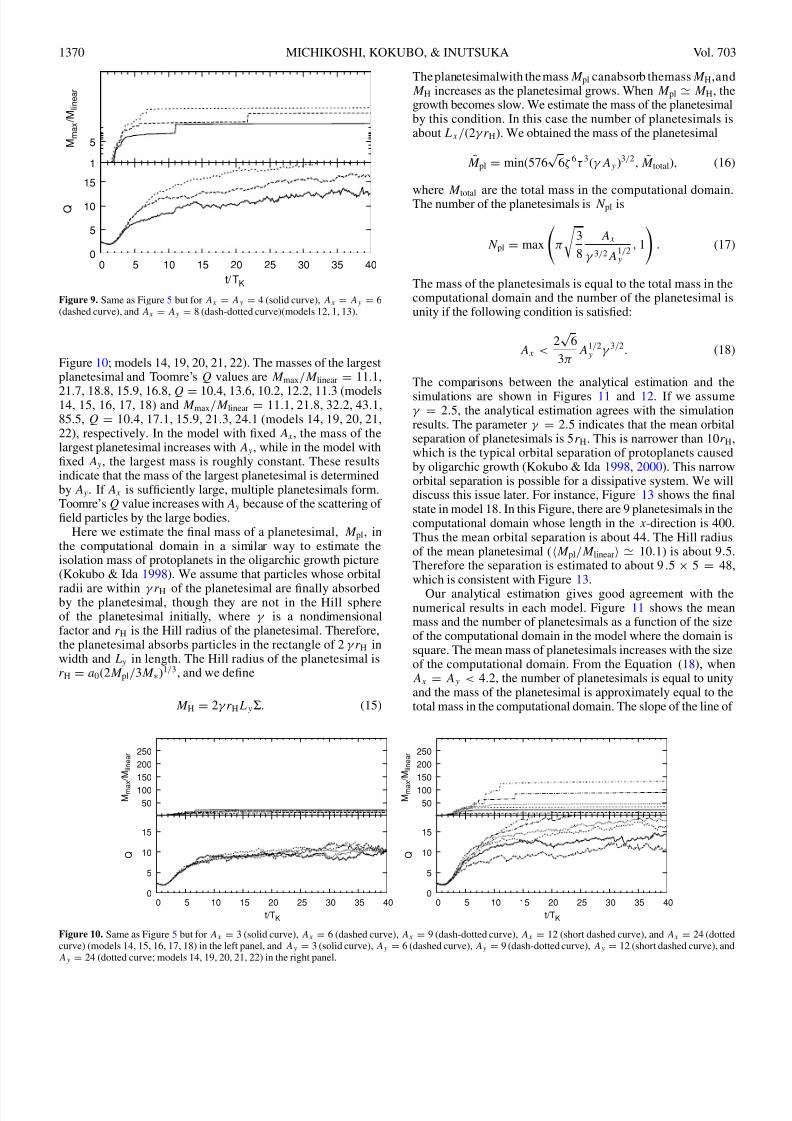
Figure 10; models 14, 19, 20, 21, 22). The masses of the largestplanetesimal and Toomre’s Q values are M max/M linear

=11.1,

21.7, 18.8, 15.9, 16.8, Q = 10.4, 13.6, 10.2, 12.2, 11.3 (models14, 15, 16, 17, 18) and M max/M linear = 11.1, 21.8, 32.2, 43.1,85.5, Q = 10.4, 17.1, 15.9, 21.3, 24.1 (models 14, 19, 20, 21,22), respectively. In the model with fixed A x, the mass of thelargest planetesimal increases with A y, while in the model withfixed A y, the largest mass is roughly constant. These resultsindicate that the mass of the largest planetesimal is determinedby A y. If  A x is sufficiently large, multiple planetesimals form.Toomre’s Q value increases with A y because of the scattering of field particles by the large bodies.

Here we estimate the final mass of a planetesimal, M pl, inthe computational domain in a similar way to estimate theisolation mass of protoplanets in the oligarchic growth picture(Kokubo & Ida 1998). We assume that particles whose orbital

radii are within γ rH of the planetesimal are finally absorbedby the planetesimal, though they are not in the Hill sphereof the planetesimal initially, where γ  is a nondimensionalfactor and rH is the Hill radius of the planetesimal. Therefore,the planetesimal absorbs particles in the rectangle of 2γ rH inwidth and L y in length. The Hill radius of the planetesimal isrH = a0(2M pl/3M ∗)1/3, and we define

M H = 2γ rHLyΣ. (15)

The planetesimalwith the massM pl canabsorb themass M H,andM H increases as the planetesimal grows. When M pl M H, thegrowth becomes slow. We estimate the mass of the planetesimalby this condition. In this case the number of planetesimals isabout Lx /(2γ rH). We obtained the mass of the planetesimal

M pl = min(576√ 

6ζ 6τ 3(γ Ay )3/2, M total), (16)

where M total are the total mass in the computational domain.The number of the planetesimals is N pl is

N pl = max

π

3

8

Ax

γ 3/2A1/2y

, 1

. (17)

The mass of the planetesimals is equal to the total mass in thecomputational domain and the number of the planetesimal isunity if the following condition is satisfied:

Ax <2√ 

6

3πA1/2

y γ 3/2. (18)

The comparisons between the analytical estimation and the

simulations are shown in Figures 11 and 12. If we assumeγ  = 2.5, the analytical estimation agrees with the simulationresults. The parameter γ  = 2.5 indicates that the mean orbitalseparation of planetesimals is 5rH. This is narrower than 10rH,which is the typical orbital separation of protoplanets causedby oligarchic growth (Kokubo & Ida 1998, 2000). This narroworbital separation is possible for a dissipative system. We willdiscuss this issue later. For instance, Figure 13 shows the finalstate in model 18. In this Figure, there are 9 planetesimals in thecomputational domain whose length in the x-direction is 400.Thus the mean orbital separation is about 44. The Hill radiusof the mean planetesimal (M pl/M linear 10.1) is about 9.5.Therefore the separation is estimated to about 9.5 × 5 = 48,which is consistent with Figure 13.

Our analytical estimation gives good agreement with thenumerical results in each model. Figure 11 shows the meanmass and the number of planetesimals as a function of the sizeof the computational domain in the model where the domain issquare. The mean mass of planetesimals increases with the sizeof the computational domain. From the Equation (18), whenAx = Ay < 4.2, the number of planetesimals is equal to unityand the mass of the planetesimal is approximately equal to thetotal mass in the computational domain. The slope of the line of 

0

5

10

15

0 5 10 15 20 25 30 35 40

   Q

t/TK

50

100

150

200

250

   M  m  a

  x   /   M   l   i  n  e  a  r

0

5

10

15

0 5 10 15 20 25 30 35 40

   Q

t/TK

50

100

150

200

250

   M  m  a

  x   /   M   l   i  n  e  a  r

Figure 10. Same as Figure 5 but for Ax = 3 (solid curve), Ax = 6 (dashed curve), Ax = 9 (dash-dotted curve), Ax = 12 (short dashed curve), and Ax = 24 (dottedcurve) (models 14, 15, 16, 17, 18) in the left panel, and Ay = 3 (solid curve), Ay = 6 (dashed curve), Ay = 9 (dash-dotted curve), Ay = 12 (short dashed curve), andAy = 24 (dotted curve; models 14, 19, 20, 21, 22) in the right panel.

8/4/2019 N-Body Self Gravity

http://slidepdf.com/reader/full/n-body-self-gravity 9/11

No. 2, 2009 FORMATION OF PLANETESIMALS. II. 1371

1

10

100

1000

1 10

      ⟨   M  p   l      ⟩   /   M   l   i  n  e  a  r

A

0.1

1

10

100

1 10

   N  p   l

A

Figure 11. Averaged mass M pl (left panel) and the number N pl (right panel) of the planetesimals as a function of the size of the computational domainA = Ax = Ay = 4, 6, 8 (models 12, 1, 13). The solid line denotes the analytical estimation given by Equations (16) and (17). We set γ  = 2.5. The error barshows the range of planetesimal masses in a given run.

1

10

100

1000

1 10

      ⟨   M  p   l      ⟩   /   M   l   i  n  e  a  r

A

0.1

1

10

100

1 10

   N  p   l

A

Figure 12. Same as Figure 11 but for A = Ax = 3, 6, 9, 12, 24 (cross points; models 14, 15, 16, 17, 18) and A = Ay = 3, 6, 9, 12, 24 (plus points; models 14, 19,20, 21, 22). The dotted and solid lines denote the analytical estimations given by Equations (16) and (17).

Figure 13. Spatial distribution of particles in model 18 at t  = 40T K . The meanplanetesimal mass is about M pl/M linear 10 and its Hill radius is about 9.5.

the mean mass of planetesimals changes at Ax = Ay = 4.2and the number of the planetesimals is larger than unity if 

Ax = Ay > 4.2.Figure 12 shows the result for the model of the rectangular

computational domain. In the models of Ay = 3, the mean massof planetesimals is constant and the number of planetesimalsis larger than unity if  Ax > 3.6. In the models of  Ax = 3,the slopes of the lines change at Ay = 2.1. The growthof planetesimals cannot be saturated although A y is large. Inthese models, the Hill radius of the planetesimal is longerthan the size of the computational domain in the x-direction.The only one planetesimal forms, and it absorbs most mass inthe computational domain. It should be remembered that thelocal calculation of planetesimal formation has the domain-sizedependence.

If we assume that the surface density of dust is

Σ = 10 × f d

a0

1 AU

−3/2

g cm−2, (19)

where f d is a scaling factor, the linear mass M linear is given by

M linear = 3.5 × 1018f 3d

a0

1 AU

3/2

M ∗M 

−2

g, (20)

and from Equation (16) the estimated planetesimal mass M pl isgiven by

M pl = 9.0 × 1018f 3d a0

1 AU3/2 M 

∗M 

−2 γ 

2.53/2

A3/2y g

= 2.6 γ 

2.5

3/2

A3/2y M linear, (21)

where we assume Ax > 2.1A1/2y (γ /2.5)3/2. The factor f d = 1

roughly corresponds to the minimum mass solar nebula modelinside the snow line (Hayashi 1981). From Equation (21), theestimated planetesimalmass becomes larger than the linear massif the feeding zone is large, (Ay γ )3/2 > 1.6.

The estimated and linear masses exhibit the same dependen-cies on f d, a0, and M ∗, and the estimated planetesimal mass ison the same order of the linear mass when Ay γ  1. These

8/4/2019 N-Body Self Gravity

http://slidepdf.com/reader/full/n-body-self-gravity 10/11

1372 MICHIKOSHI, KOKUBO, & INUTSUKA Vol. 703

results are explained as follows. Here we rewrite the Hill radiusby the most unstable wavelength

rH = λmost

(3π)1/3

M pl

M linear

1/3

, (22)

where the most unstable wavelength for Q = 1 is

λmost =2π 2GΣ

Ω20

. (23)

The most unstable wavelength of the gravitational instabilityand the Hill radius of the linear mass are on the same order.The condition Q = 1 corresponds to the balance between theself-gravity and the effect of the rotation. On the other hand, theHill radius is determined by the balance between theself-gravityand the tidal force. Thus, rH and λmost are on the same order, andthe planetesimal mass is on the order of the linear mass only if Ay γ  1. In general, because Ay 1, the planetesimal massis larger than the linear mass.

Collisions among planetesimals are more frequent than therealistic case in the present simulations since the bulk density of super-particle is much smaller than the realistic value. Thereforethe orbital separation of large planetesimals is different from thatof the standard oligarchic growth derived by N -body simulationsof planetesimals (Kokubo & Ida 1998, 2000). If the numberdensity is low, theorbital separation is determined by thebalancebetween the orbital repulsion and their growth (Kokubo & Ida1998). But if the number density is high, and the collisionaldissipation is effective, the orbital repulsion is relatively weak.Thus, in the collisional oligarchic growth, the orbital separationcan be narrower than 10RH (Goldreich et al. 2004).

4. SUMMARY

We performed local N -body simulations of planetesimal for-mation through gravitational instability and collisional growth

without a gas component using a shearing box method. Theaccretion model was adopted as the collision model. In the ac-cretion model, when particles collide, if the binding condition issatisfied, two particles merge into one. The number of particlesdecreases as the calculation proceeds; thus, this model enablesus to perform the long-term and large-scale calculations. Wecompared the results of the accretion model with those of thehard and soft sphere models used in Paper I.

The formation process of planetesimals is the same as that of the hard and soft sphere models. It is divided into three stages:the formation of nonaxisymmetric structures; the creation of planetesimal seeds; and the collisional growth of the planetes-imals. The velocity dispersion of particles decreases graduallydue to the inelastic collisions. The gravitational instability oc-

curs when the velocity dispersion of particles becomes a criticalvalue determined by Q 2. The nonaxisymmetric structuresform and fragment into planetesimal seeds, the masses of whichare on the order of the linear mass. In this paper, we consider theformation of nonaxisymmetric structures and planetesimalseedsas gravitational instability. Planetesimal seeds grow rapidly bycoagulation and the large planetesimals form. Most of the massin the computational domain is absorbed by a few large plan-etesimals.

We studied the effect of physical parameters on planetesimalformation: the restitution coefficient , the initial optical depthτ , the dependence of planetesimal formation on the ratioζ = rH/2rp, and the initial Toomre’s Q value. We found

no qualitative differences among the collision models. In theaccretion model, the merged particles cannot split; thus, thegrowth of particles is more efficient than in the hard and softsphere models. If the restitution coefficient is smaller than thecritical value, thetime evolution is similar to thestandard model.If τ  is large,the collisionfrequency is high, andthe dissipation of the kinetic energy is efficient. Thus, the gravitational instabilityoccurs more quickly for larger τ . In this narrow parameter rangeζ

=2.5, 2.75, 3.0, there is no remarkable dependence on ζ .

By the long-term and large-scale calculations using the accre-tion model, we found that the mean mass of the planetesimalsdepends on the size of the computational domain. We found that

the mean mass of planetesimals is proportional to L3/2y . How-

ever, this mass is independent of  L x if  L x is sufficiently large.The mean mass of planetesimals is estimated by Equation (16).Large planetesimals sweep small planetesimals in the rotationaldirection. If the orbital separation of planetesimals is sufficientlylarge, the planetesimals cannot collide. The typical orbital sepa-ration is about 5rH in the present simulation The dependence of the planetesimal mass on the size of the computational domainindicates that we cannot simply discuss the realistic mass of theplanetesimal using the local calculation.

The effect of gas was neglected in our simulation in orderto study the physical process of gravitational instability of dustparticles and subsequent collisional evolution as a first step.Once gravitational instability happens and large aggregatesform, we may be able to neglect gas drag because they areso large that they decouple from gas. So our gas-free modelmay be applicable to the stages of gravitational instabilityand subsequent collisional growth. The simple gas-free modelprovides thorough understanding of the gravitational instabilityand collisional growth of planetesimals. However, it is necessaryto include gas drag so as to investigate the realistic formationprocess of planetesimals, since the stopping time of small dustparticles is shorter than the Kepler time. We will investigate thegravitational instability of a particle disk embedded in a laminar

gaseous disk in the next paper.

The authors thank the anonymous referee for helpful com-ments and suggestions. This research was partially supportedby MEXT (Ministry of Education, Culture, Sports, Scienceand Technology), Japan, the grant-in-aid for Scientific Researchon Priority Areas, “Development of Extra-Solar Planetary Sci-ence,” and the Special Coordination Fund for Promoting Sci-ence and Technology, “GRAPE-DR Project.” S.I. is supportedby grants-in-aid (15740118, 16077202, and 18540238) fromMEXT of Japan.

REFERENCES

Adachi, I., Hayashi, C., & Nakazawa, K. 1976, Prog. Theor. Phys., 56, 1756Balbus, S. A., & Hawley, J. F. 1991, ApJ, 376, 214Barge, P., & Sommeria, J. 1995, A&A, 295, L1Canup, R. M., & Esposito, L. W. 1995, Icarus, 113, 331Champney, J. M., Dobrovolskis, A. R., & Cuzzi, J. N. 1995 , Phys. Fluids, 7,

1703Coradini, A., Magni, G., & Federico, C. 1981, A&A, 98, 173Cuzzi, J. N., Dobrovolskis, A. R., & Champney, J. M. 1993 , Icarus, 106, 102Daisaka, H., & Ida, S. 1999, Earth, Planets, Space, 51, 1195Daisaka, H., Tanaka, H., & Ida, S. 2001, Icarus, 154, 296Dobrovolskis, A. R., Dacles-Mariani, J. S., & Cuzzi, J. N. 1999,

J. Geophys. Res., 104, 30805Fromang, S., & Nelson, R. P. 2006, A&A, 457, 343Goldreich, P., Lithwick, Y., & Sari, R. 2004, ARA&A, 42, 549Goldreich, P., & Tremaine, S. 1982, ARA&A, 20, 249Goldreich, P., & Ward, W. R. 1973, ApJ, 183, 1051

8/4/2019 N-Body Self Gravity

http://slidepdf.com/reader/full/n-body-self-gravity 11/11

No. 2, 2009 FORMATION OF PLANETESIMALS. II. 1373

Hayashi, C. 1981, Prog. Theor. Phys. Suppl., 70, 35Ida, S., & Makino, J. 1992, Icarus, 96, 107Ishitsu, N., & Sekiya, M. 2002, Earth, Planets, and Space, 54, 917Ishitsu, N., & Sekiya, M. 2003, Icarus, 165, 181Johansen, A., Henning, T., & Klahr, H. 2006a, ApJ, 643, 1219Johansen, A., Klahr, H., & Henning, T. 2006b, ApJ, 636, 1121Johansen, A., Oishi, J. S., Low, M.-M. M., Klahr, H., Henning, T., & Youdin,

A. 2007, Nature, 448, 1022Kokubo, E., & Ida, S. 1998, Icarus, 131, 171Kokubo, E., & Ida, S. 2000, Icarus, 143, 15

Makino, J., Fukushige, T., Koga, M., & Namura, K. 2003, PASJ, 55,1163Michikoshi, S., & Inutsuka, S.-i. 2006, ApJ, 641, 1131Michikoshi, S., Inutsuka, S.-i., Kokubo, E., & Furuya, I. 2007, ApJ, 657,

521Nakazawa, K., & Ida, S. 1988, Prog. Theor. Phys. Suppl., 96, 167Ohtsuki, K. 1993, Icarus, 106, 228Ohtsuki, K. 1999, Icarus, 137, 152Ohtsuki, K., & Emori, H. 2000, AJ, 119, 403Petit, J.-M., & Henon, M. 1986, Icarus, 66, 536Richardson, D. C. 1994, MNRAS, 269, 493

Safronov, V. 1969, Evolution of the Protoplanetary Cloud and Formation of theEarth and Planets (Moscow: NASA Tech. Trans. TT-F-677)

Salo, H. 1991, Icarus, 90, 254Salo, H. 1995, Icarus, 117, 287Sekiya, M. 1983, Prog. Theor. Phys., 69, 1116Sekiya, M. 1998, Icarus, 133, 298Sekiya, M., & Ishitsu, N. 2000, Earth, Planets, Space, 52, 517Sekiya, M., & Ishitsu, N. 2001, Earth, Planets, Space, 53, 761Tanga, P., Weidenschilling, S. J., Michel, P., & Richardson, D. C. 2004 , A&A,

427, 1105

Ward, W. R. 1976, in Frontiers of Astrophysics, ed. E. H. Avrett (Cambridge,MA: Harvard Univ. Press), 1Weidenschilling, S. J. 1977, MNRAS, 180, 57Weidenschilling, S. J. 1980, Icarus, 44, 172Weidenschilling, S. J. 1995, Icarus, 116, 433Weidenschilling, S. J., & Cuzzi, J. N. 1993, in Protostars and Planets III, ed.

E. H. Levy & J. I. Lunine (Tucson, AZ: Univ. Arizona Press), 1031Wisdom, J., & Tremaine, S. 1988, AJ, 95, 925Youdin, A. N. 2005a, arXiv:astro-ph/0508659Youdin, A. N. 2005b, arXiv:astro-ph/0508662Youdin, A. N., & Goodman, J. 2005, ApJ, 620, 459