Multiple-Output Modelling for Multi-Step-Ahead Time SeriesForecasting

Souhaib Ben Taieba, Antti Sorjamaab, Gianluca Bontempia

aMachine Learning Group, Departement d’Informatique, Faculte des Sciences, Universite Libre de Bruxelles, BelgiumbTime Series Prediction and Chemoinformatics, Adaptive Informatics Research Centre, Helsinki University of

Technology, Finland

Abstract

Accurate prediction of time series over long future horizons is the new frontier of forecasting.

Conventional approaches to long-term time series forecasting rely either on iterated one-step-

ahead predictors or direct predictors.

In spite of their diversity, iterated and direct techniques for multi-step-ahead forecasting share

a common feature, i.e. they model from data a multiple-input single-output mapping. In previous

works, the authors presented an original multiple-output approach to multi-step-ahead prediction.

The goal is to improve accuracy by preserving in the forecasted sequence the stochastic properties

of the training series. This is not guaranteed for instance in direct approaches where predictions

for different horizons are performed independently.

This paper presents a review of single-output vs. multiple-output approaches for prediction

and goes a step forward with respect to the previous authors contributions by (i) extending the

multiple-output approach with a query based criterion and (ii) presenting an assessment of single-

output and multiple-output methods on the NN3 competition datasets.

In particular, the experimental section shows that multiple-output approaches represent a

competitive choice for tackling long-term forecasting tasks.

Key words: Long-Term Time Series Prediction, Multiple-output Models, Lazy Learning, NN3

Prediction Competition

1. Introduction

The prediction of the future behavior of an observed time series {ϕ1, . . . , ϕN} over a long

horizon H is still an open problem in forecasting [26]. Currently, the most common approaches

to long-term forecasting rely either on iterated or direct prediction techniques [18, 23].Preprint submitted to Neurocomputing December 13, 2010

In iterated methods, an H-step-ahead prediction problem is tackled by iterating, H times, a

one-step-ahead predictor. Once the predictor has estimated the future series value, this value is

fed back as an input to the following prediction. Hence, the predictor takes estimated values

as inputs, instead of actual observations with evident negative consequences in terms of error

propagation. Examples of iterated approaches are recurrent neural networks [27] or local learning

iterated techniques [15, 20].

Direct methods perform H-step-ahead forecasting by estimating a set of H prediction models,

each returning a direct forecast of ϕN+h with h ∈ {1, . . . ,H} [23]. Direct methods often require

higher functional complexity than iterated ones in order to model the stochastic dependency

between two series values at two distant instants.

In computational intelligence literature, we have also examples of research works, where the

two approaches have been successfully combined [22].

In spite of their diversity, iterated and direct techniques for multi-step-ahead prediction share

a common feature: they model from data, a multiple-input single-output mapping, where the

outputs are the variable ϕN+1 in the iterated case and the variable ϕN+h in the direct case, respec-

tively.

In [5], the author proposed a Multiple-Input Multiple-Output (MIMO) approach for multi-

step-ahead time series prediction, where the predicted value is not a scalar quantity but a vector

of future values {ϕN+1, . . . , ϕN+H} of the time series ϕ. This approach replaces the H models

of the Direct approach by one multiple-output model, with the goal of preserving, among the

predicted values, the stochastic dependency characterizing the time series. Note that, though the

multivariate responses prediction is well-studied in stastical learning theory [9], what is novel

here is its application to multi-step-ahead time series forecasting.

The Direct and the MIMO approach can be indeed seen as two distinct instances of the same

prediction approach, which decomposes long-term prediction into multiple-output tasks. In the

direct case, the number of prediction tasks is equal to the size of the horizon H and the size of the

outputs is 1. In the MIMO case, the number of prediction tasks is equal to one and the size of the

output is H. Intermediate configurations can be imagined by transforming the original task into

n = Hs prediction tasks, each with multiple outputs of size s, where s ∈ {1, . . . ,H}. This approach,

called Multiple-Input Several Multiple-Outputs (MISMO) was first introduced in [25] and trades

off the property of preserving the stochastic dependency between future values with a greater

2

flexibility of the predictor. For instance, the fact of having n > 1 different models allows the

selection of different inputs for different horizons. In other terms, s addresses the bias/variance

trade-off of the predictor by constraining the degree of dependency between predictions (null in

the case s = 1 and maximal for s = H).

This paper aims to provide a review of the existing multiple-output approaches to time series

prediction and to compare them to conventional single-output approaches. Also it brings two

original contributions to the existing literature, notably (i) an extension of the MISMO method-

ology by considering an additional query-based criterion for selecting the optimal size of the

output vector and (ii) an extensive assessment of multiple-output and single output strategies by

testing them on 111 series of the NN3 international competition benchmark.

Note that, in order to setup a common and reliable benchmark, we adopt here the same local

learning algorithm, Lazy Learning [3, 7], to implement the different prediction strategies. As

shown in the previous contributions, the Lazy Learning algorithm returns accurate predictions

both in a single-output [8, 6] and a multiple-output context [5, 25]. Lazy Learning (LL) is a local

modeling technique, which is query-based in the sense that the whole learning procedure (i.e.

structural and parametric identification) is deferred until a prediction is required. In particular

we will adopt the LL algorithm presented in [3, 7] that selects on a query-by-query basis and by

means of a local cross-validation scheme the optimal number of neighbors.

2. Multi-step-ahead Prediction Techniques

Given a time series {ϕ1, . . . , ϕN} composed of N observations, multi-step-ahead prediction

consists of predicting {ϕN+1, . . . , ϕN+H}, the H next values of the time series, where H > 1 is the

prediction horizon.

This section introduces the main characteristics of two families of prediction strategies:

the Single-Output stategy which relies on the estimation of a single-output predictor and the

Multiple-Output strategy, which learns from data a multiple-input multiple-output dependency

between a window of past observations and a window of future values.

2.1. Single-Output Prediction Strategy

Conventional approaches to multi-step-ahead prediction [11, 24], like iterated and direct

methods, belong to this family since they both model from data a multiple-input single-output

3

mapping. Their difference resides in the considered output variable: ϕN+1 in the iterated case and

the variables ϕN+h, h = 1, . . . ,H in the direct case. In the following sections we will provide a

common notation to introduce and discuss these two approaches.

2.1.1. Iterated method

The iterated method is the oldest technique to carry out multi-step-ahead prediction [23]. In

this method, once a one-step-ahead prediction is computed, the value is fed back as an input to

the following step. The iterated method demands to fit from historical data the Nonlinear Auto

Regressive (NAR) dependency [14]

ϕt+1 = f (ϕt, ϕt−1, . . . , ϕt−d+1) + w, (1)

where w is the scalar zero-mean noise term and d is the embedding dimension [10], that is the

number of past values taken into consideration to predict one future value.

After the learning process, the estimation of the H next values is returned by

ϕN+h =

f (ϕN , . . . , ϕN−d+1) if h = 1

f (ϕN+h−1, . . . , ϕN+1, ϕN , . . . , ϕN−d+h) if h ∈ {2, . . . , d}

f (ϕN+h−1, . . . , ϕN+h−d) if h ∈ {d + 1, . . . ,H}

(2)

Iterated methods may suffer from low performance in long horizon tasks. This is due to the

fact that they are essentially models tuned with a one-step-ahead criterion and therefore, they

doesn’t take the temporal behavior into account appropriately. Moreover, the predictor takes

approximated values as inputs instead of actual observations, which leads to the propagation of

the prediction error.

Examples of iterated approaches are recurrent neural networks [27] or local learning iterated

techniques [15, 20].

2.1.2. Direct method

The Direct method is an alternative method for long-term prediction. It learns H single-

output models fh where

ϕt+h = fh(ϕt, ϕt−1, . . . , ϕt−d+1) + w, (3)

4

with h ∈ {1, . . . ,H}.

After the learning process, the estimations of the H next values are given by

ϕN+h = fh(ϕN , . . . , ϕN−d+1). (4)

An attractive property of this method is that it is not prone to the accumulation of the pre-

diction errors [23]. However, the fact that the H models are learned independently induces a

conditional independence of the H estimators ϕN+h. This prevents the technique from consider-

ing complex dependencies between the variables ϕt+h and consequently bias the prediction accu-

racy. A possible way to remedy this shortcoming is to move from the modeling of single-output

mapping to the modeling of multiple-output dependencies.

2.2. Multiple-Output Prediction Strategy

In order to remove the conditional independence assumption which is implicit in the Direct

approach, we can adopt a Multiple-Output strategy for multi-step ahead prediction. In this sec-

tion, two instances of this Multiple-Output strategy are introduced: the MIMO and the MISMO

method [25].

2.2.1. MIMO method

The MIMO method consists in using historical data to learn one multiple-output dependency

F where

{ϕt+H , . . . , ϕt+1} = F(ϕt, ϕt−1, . . . , ϕt−d+1) + w (5)

and w is a vector noise term of zero mean and non diagonal covariance.

After the learning process, the estimation of the H next values are given by

{ϕN+H , . . . , ϕN+1} = F(ϕN , ϕN−1, . . . , ϕN−d+1) (6)

Note that in this case the returned prediction is not a scalar but a time series itself. In case of

large horizon H, the number of terms could be enough to allow the use of specific operators of

time series analysis (for instance autocorrelation or partial autocorrelation) [25].

The MIMO method constrains all the horizons to be predicted with the same model struc-

ture, for instance with the same set of inputs, and by using the same learning procedure. This

constraint greatly reduces the flexibility and the variability of the single-output approaches and

it could produce the negative effect of biasing the returned model.5

2.2.2. MISMO method

A solution to the shortcomings of the previously discussed techniques comes from the adop-

tion of an intermediate approach, where the constraint of MIMO is relaxed by tuning an integer

parameter s, which calibrates the dimensionality of the output on the basis of a validation crite-

rion. The MISMO method, first introduced in [25], aims to learn from data n = Hs multiple-output

dependencies Fp where

{ϕt+ps, . . . , ϕt+(p−1)s+1} = Fp(ϕt, ϕt−1, . . . , ϕt−d+1) + w, p ∈ {1, . . . , n} (7)

and w is a zero-mean vector of size s. In other terms, s represents the number of consecutive

outputs to be predicted at a time by a multiple-output model.

After the learning process, the estimation of the H next values are returned by the n steps

{ϕN+ps, . . . , ϕN+(p−1)s+1} = Fp(ϕN , ϕN−1, . . . , ϕN−d+1), p ∈ {1, . . . , n} (8)

The MISMO approach addresses the multi-step-ahead problem by taking into consideration

two aspects: future predictions are expected to be dependent because of the stochastic properties

of the series but at the same time their degree of dependency is difficult to set a priori and typically

not related to the horizon H fixed by the user. Think for example a NAR process of order d = 2

where a H = 50 ahead predictions is needed. In this case a MIMO model (i.e. s = 50) is

extremely biased since it forces dependencies in the output with an order much bigger than 2.

However, the increased MISMO adaptivity comes at the cost of an additional parameter s,

which has to be carefully chosen on the basis of data. The following section will detail how to

deal with this issue in a forecasting context.

3. The Proposed Methodology

Forecasting methods rely on learning procedures to estimate the temporal stochastic depen-

dencies from data (e.g. represented by the function f in Equation (1)). In this work, we will

consider only local learning approaches. The use of local learning approaches in forecasting

literature dates back to the seminal work of Lorenz [19] on chaotic series. Other classical refer-

ences are [15, 16, 17]

Here we will consider a local learning approach where the problem of adjusting the size

of the neighborhood is solved by a Lazy Learning (LL) algorithm [7]. This algorithm selects6

on a query-by-query basis and by means of a local cross-validation scheme the best number of

neighbors. In what follows, we will first review the local learning procedure for a conventional

single-output problem and we will then extend the methodology to MIMO and MISMO settings.

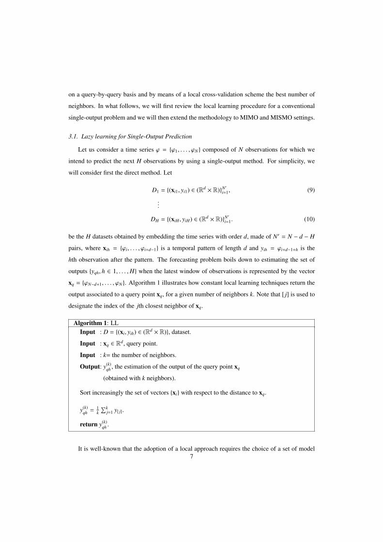
3.1. Lazy learning for Single-Output Prediction

Let us consider a time series ϕ = {ϕ1, . . . , ϕN} composed of N observations for which we

intend to predict the next H observations by using a single-output method. For simplicity, we

will consider first the direct method. Let

D1 = {(xi1, yi1) ∈ (Rd × R)}N′

i=1, (9)

...

DH = {(xiH , yiH) ∈ (Rd × R)}N′

i=1. (10)

be the H datasets obtained by embedding the time series with order d, made of N′ = N − d − H

pairs, where xih = {ϕi, . . . , ϕi+d−1} is a temporal pattern of length d and yih = ϕi+d−1+h is the

hth observation after the pattern. The forecasting problem boils down to estimating the set of

outputs {yqh, h ∈ 1, . . . ,H} when the latest window of observations is represented by the vector

xq = {ϕN−d+1, . . . , ϕN}. Algorithm 1 illustrates how constant local learning techniques return the

output associated to a query point xq, for a given number of neighbors k. Note that [ j] is used to

designate the index of the jth closest neighbor of xq.

Algorithm 1: LLInput : D = {(xi, yih) ∈ (Rd × R)}, dataset.

Input : xq ∈ Rd, query point.

Input : k= the number of neighbors.

Output: y(k)qh , the estimation of the output of the query point xq

(obtained with k neighbors).

Sort increasingly the set of vectors {xi} with respect to the distance to xq.

y(k)qh = 1

k∑k

j=1 y[ j].

return y(k)qh .

It is well-known that the adoption of a local approach requires the choice of a set of model7

parameters (e.g. the number k of neighbors, the kernel function, the distance metric) [2]. In this

paper, we will adopt a constant kernel, an euclidean distance and we will select the number of

neighbors by a Leave-One-Out (LOO) criterion.

A computationally efficient way to perform LOO cross-validation and to assess the per-

formance in generalization of local linear models is the PRESS statistic, proposed in 1974 by

Allen [1]. By assessing the performance of each local model, alternative configurations can be

tested and compared in order to select the best one in terms of expected prediction. The idea

consists in associating a LOO error eLOO(k) to the estimation

y(k)q =

1k

k∑j=1

y[ j], (11)

associated to the query point xq and returned by k neighbors. In case of a constant model, the

LOO term can be derived as follows [4]:

eLOO(k) =1k

k∑j=1

(e j(k))2, (12)

where

e j(k) = y[ j] −

∑ki=1(i, j) y[i]

k − 1= k

y[ j] − yk

k − 1. (13)

The best number of neighbors is then defined as the number

k∗ = arg mink∈{2,...,K} eLOO(k), (14)

which minimizes the LOO error.

In the following, LL will refer to a constant Lazy Learner which selects the number of neigh-

bors according to the LOO assessment (12). In particular we will use the acronym LL-ITER to

denote a LL iterated predictor and LL-DIRECT to denote a LL direct predictor.

3.2. Lazy Learning for MIMO Prediction

In the MIMO approach, the time series is embedded as a dataset

D = {(xi, yi) ∈ (Rd × RH)}N′

i=1, (15)

made of N′ pairs, where xi = {ϕi, . . . , ϕi+d−1} is a temporal pattern of length d and yi = {ϕi+d, . . . , ϕi+d+H−1}

is the consecutive temporal pattern of length H.

8

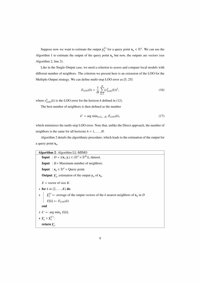
Suppose now we want to estimate the output y(k)q for a query point xq ∈ Rd. We can use the

Algorithm 1 to estimate the output of the query point xq but now, the outputs are vectors (see

Algorithm 2, line 2).

Like in the Single-Output case, we need a criterion to assess and compare local models with

different number of neighbors. The criterion we present here is an extension of the LOO for the

Multiple-Output strategy. We can define multi-step LOO error as [5, 25]

ELOO(k) =1H

H∑h=1

(ehLOO(k))2, (16)

where ehLOO(k) is the LOO error for the horizon h defined in (12).

The best number of neighbors is then defined as the number

k∗ = arg mink∈{2,...,K} ELOO(k), (17)

which minimizes the multi-step LOO error. Note that, unlike the Direct approach, the number of

neighbors is the same for all horizons h = 1, . . . ,H.

Algorithm 2 details the algorithmic procedure, which leads to the estimation of the output for

a query point xq.

Algorithm 2: Algorithm LL-MIMOInput : D = {(xi, yi) ∈ (Rd × RH)}, dataset.

Input : K= Maximum number of neighbors.

Input : xq ∈ Rd = Query point.

Output: y∗q, estimation of the output yq of xq.

E = vector of size K.

for k in {2, . . . ,K} do1

y(k)q ← average of the output vectors of the k nearest neighbors of xq in D2

E[k]← ELOO(k)

end

k∗ ← arg mink E[k].3

y∗q = y(k∗)q .4

return y∗q.

9

3.3. Lazy Learning for MISMO Prediction

In addition to the number of neighbors, the MISMO method requires to tune the parame-

ter s (Section 2.2.2), which addresses the bias/variance trade-off by constraining the degree of

dependency between the predictions.

We will propose two strategies to choose s, a query-independent strategy (denoted LL-

MISMO-G and already introduced in [25]) and an original strategy (denoted LL-MISMO-L)

which relies on a query-based selection .

3.3.1. LL-MISMO-G

This strategy consists in assessing the performance of the MISMO method for different values

of the parameter s by cross-validation on the entire learning set, and then making the selection

(Algorithm 3). After the selection, the parameter s is fixed for all query points (Algorithm 4).

In Algorithm 3, the first loop (line 1) ranges over all the values of the parameter s. Given a

value of the parameter s, the output y is divided into n = Hs portions (yi1, · · · , yin). The second

loop (line 2) processes each portion separately by measuring the LOO error (see Algorithm 2)

for a number k ∈ {2, . . . ,K} of neighbors. For each p ∈ {1, . . . , n}, we obtain a LOO error vector

E(p)learning of size K. The average of E(p)

learning over p is denoted by Elearning(s) and its kth term

represents the LOO performance of the MISMO model with the parameter s and k neighbors.

Note that several alternatives could be used to derive a global (i.e. independent of the number of

neighbors) estimate Error(s) of the MISMO performance for a given s. For instance, we could

take the mean (line 3) or the minimum (line 4) value of the vector Elearning(s).

Once the value s∗ is computed, it is passed to the Algorithm 4. The loop (line 1) processes

each portions separately by calling the LL-MIMO Algorithm 2. Note that the best number of

neighbors can be different for each portion because the learning process is made independently

for each portion. After calculating the prediction for each portion, the output of the query point

xq is obtained by the concatenated vector {y∗q1, . . . , y∗qn}.

3.3.2. LL-MISMO-L

We present here an original query-based strategy where the selection of the parameter s (e.g.

the size of the multiple outputs) is a function of the current query point. For each query point,

LL-MISMO-L (Algorithm 5) computes the LOO error associated to different values of s and

10

Algorithm 3: Selection of the best value of the parameter sInput : D = {(xi, yi) ∈ (Rd × RH)}N

′

i=1, dataset.

Input : K= Maximum number of neighbors.

Output: s∗= Best value of the parameter s

for s in {1, . . . ,H} do1

n = Hs

for p in {1, . . . , n} do2

D(s)p = {(xip, yip) ∈ (Rd × Rs)}

E(p)learning = vector of size K

for k in {2, . . . ,K} doE(p)

learning[k]← LL-MIMO error by using D(s)p and the range {2, . . . , k}

end

end

Elearning(s) = vector of size K

for k in {2, . . . ,K} doElearning(s)[k]← 1

n∑n

p=1 E(p)learning[k]

end

Errormean(s)← 1K∑K

k=2 Elearning(s)[k]3

Errormin(s)← min(Elearning(s)[k])4

end

s∗ = arg mins∈{1,...,H} Errormean(s) (Minimum criterion)

or

s∗ = arg mins∈{1,...,H} Errormin(s) (Mean criterion)

return s∗

11

Algorithm 4: Algorithm LL-MISMO-GInput : D = {(xi, yi) ∈ (Rd × RH)}N

′

i=1, dataset.

Input : K= Maximum number of neighbors.

Input : s∗= Best value of the parameter s (see Algorithm 3).

Input : xq ∈ Rd = Query point.

Output: y∗q, estimation of the output yq of xq.

n = Hs∗

for p in {1, . . . , n} do1

Dp = {(xip, yip) ∈ (Rd × Rs∗ )}

y∗qp =LL-MIMO(Dp,K,xq) (see Algorithm 2)2

end

y∗q = {y∗q1, . . . , y∗qn}3

return y∗q

selects the best one. This means that the strategy is lazy not only in terms of neighbor selection

but also in terms of the selection of s.

The first loop (line 1) ranges over all the values of the parameter s. Inside the loop, for a

given a value of the parameter s, the output y is divided into n = Hs portions (yi1, · · · , yin). The

second loop (line 2) processes each portions separately by estimating the outputs of the query xq

for each portion with a number k ∈ {2, . . . ,K} of neighbors.

A LOO error E(p)[k] is associated to each estimation y(k)qp obtained with k neighbors, for each

portion p. For a given value of the parameter s, a prediction yq(s) = {y∗q1(s), . . . , y∗qn(s)} (line 3)

and two error vectors (Errormin(s) or Errormean(s)) (lines 4 and 5) representing the quality of the

prediction are calculated. Finally, the prediction which minimizes the chosen error is selected as

the final prediction.

Note that this procedure takes advantage of the fast computation of the leave-one-out error in

constant local learning by using a vectorial version of PRESS (Equation 12).

12

Algorithm 5: Algorithm LL-MISMO-LInput : D = {(xi, yi) ∈ (Rd × RH)}N−d−H

i=1 , dataset.

Input : K= Maximum number of neighbors.

Input : xq ∈ Rd = Query point.

Output: y∗q, estimation of the output yq of xq.

for s in {1, . . . ,H} do1

n = Hs

for p in {1, . . . , n} do2

D(s)p = {(xip, yip) ∈ (Rd × Rs)}

E(p) = vector of size K

for k in {2, . . . ,K} doy(k)

qp ← Calculate y(k)qp by using k neighbors in D(s)

p

E(p)[k]← ELOO(k) associated to y(k)qp

end

k∗ ← arg mink E(p)[k]

y∗qp(s) = y(k∗)qp

end

yq(s) = {y∗q1(s), . . . , y∗qn(s)}3

E(s) = vector of size K

for k in {2, . . . ,K} doE(s)[k]← 1

n∑n

p=1 E(p)[k]

end

Errormean(s)← 1K∑K

k=2 E(s)[k]4

Errormin(s)← min(E(s)[k])5

end

s∗ = arg mins∈{1,...,H} Errormean(s) (Minimum criterion)

or

s∗ = arg mins∈{1,...,H} Errormin(s) (Mean criterion)

y∗q = yq(s∗)

return y∗q

13

4. Experiments

This section presents a comparison of single-output and multiple-output techniques for multi-

step-ahead prediction. In order to provide enough experimental evidence we focused on NN3 [12],

an international competition based on a large number of real time series.

4.1. Datasets and Preprocessing

The NN3 Dataset is made of 111 monthly time series starting at January, each containing

50 to 126 points. All series are drawn from homogeneous population of empirical business

time series. For each time series, the competition required to forecast the values of the next 18

months based on the given historical data points, as accurately as possible using computational

intelligence methods [12].

Figures 1 shows three time series from the NN3 dataset. As shown by the ilustrations, most

NN3 series contain a trend pattern. For that reason we preprocessed the series by detrending the

series when trends are detected by the Mann-Kendall test [21].

The learning process adopted a 10-fold cross-validation scheme to select the value of the

parameter s. The input selection was performed by means of the Delta test for the methods based

on the single-output strategy [13] and an extension of the Delta test for the methods based on the

multiple-output strategy [25] (maximum embedding order d equal to 12).

14

Time

Tim

e S

eries n

° 5

6

0 20 40 60 80 100 120 140

5500

6500

7500

Time

Tim

e S

eries n

° 6

2

0 20 40 60 80 100 120 140

1000

3000

5000

Time

Tim

e S

eries n

° 7

4

0 20 40 60 80 100 120 140

2000

5000

8000

Figure 1: Three NN3 training time series

15

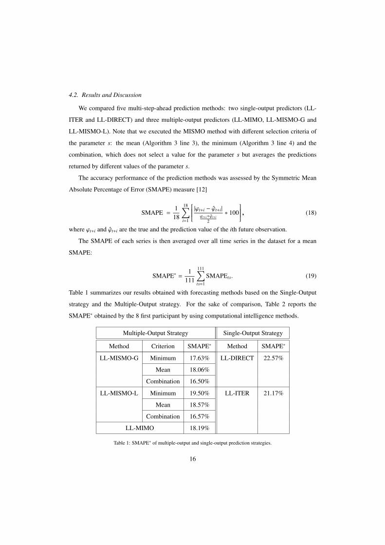
4.2. Results and Discussion

We compared five multi-step-ahead prediction methods: two single-output predictors (LL-

ITER and LL-DIRECT) and three multiple-output predictors (LL-MIMO, LL-MISMO-G and

LL-MISMO-L). Note that we executed the MISMO method with different selection criteria of

the parameter s: the mean (Algorithm 3 line 3), the minimum (Algorithm 3 line 4) and the

combination, which does not select a value for the parameter s but averages the predictions

returned by different values of the parameter s.

The accuracy performance of the prediction methods was assessed by the Symmetric Mean

Absolute Percentage of Error (SMAPE) measure [12]

SMAPE =1

18

18∑i=1

|ϕt+i − ϕt+i|

ϕt+i+ϕt+i2

∗ 100

, (18)

where ϕt+i and ϕt+i are the true and the prediction value of the ith future observation.

The SMAPE of each series is then averaged over all time series in the dataset for a mean

SMAPE:

SMAPE∗ =1

111

111∑ts=1

SMAPEts. (19)

Table 1 summarizes our results obtained with forecasting methods based on the Single-Output

strategy and the Multiple-Output strategy. For the sake of comparison, Table 2 reports the

SMAPE∗ obtained by the 8 first participant by using computational intelligence methods.

Multiple-Output Strategy Single-Output Strategy

Method Criterion SMAPE∗ Method SMAPE∗

LL-MISMO-G Minimum 17.63% LL-DIRECT 22.57%

Mean 18.06%

Combination 16.50%

LL-MISMO-L Minimum 19.50% LL-ITER 21.17%

Mean 18.57%

Combination 16.57%

LL-MIMO 18.19%

Table 1: SMAPE∗ of multiple-output and single-output prediction strategies.

16

Participant SMAPE∗ Method

Illies et al 15.18% ESN

Adeodato et al 16.17% MLP

Flores et al 16.31% GA

Chen et al 16.55% Tree

D’yakonov et al 16.57% K-NN

Kamel et al 16.92% NN+GP

Abou-Nasr 17.54% RNN

Theodosiou, Swamy 17.55% NN+theta

Table 2: SMAPE∗ obtained by the 8 first participant by using computational intelligence methods.

Table 1 shows that the methods based on the Multiple-Output strategy outperform those based

on the Single-Output strategy. Indeed, the iterated and the Direct methods provide a SMAPE∗

equal to 21.17% and 22.57% while MIMO and MISMO method return a SMAPE∗ equal to

18.19% and 16.50%, respectively.

The experiments confirm also the added value of the MISMO formulation, as shown by the

fact that MISMO returns the best SMAPE∗, equal to 16.50%. Figure 2 shows some examples of

predicted continuations returned by LL-MISMO-G.

As far as the comparison LL-MISMO-G vs. LL-MISMO-L is concerned, it appears that LL-

MISMO-G is better for all the criterion than the LL-MISMO-L Algorithm. This can be partly

explained by the fact that the LL-MISMO-L Algorithm selects two parameters locally: the num-

ber of neighbors and the value of the parameter s. In contrast, the LL-MISMO-G Algorithm first

selects the value of the parameter s globally and then selects the value of the parameter k locally.

The higher locality of LL-MISMO-L could induce higher variability and then reduce the quality

of the predictions. However the combination criterion reduces this instability and improves the

prediction accuracy (SMAPE∗=16.57%). Note that the combination is not an argument against

the assessment of different values of the parameter s since the combination of predictors with

different value of the parameter s, requires the estimation of the error for each single predictor.

Also, it is worth noting that the LL-MISMO-L algorithm does not require a complex vali-

dation procedure to select the best value of the parameter s, which makes its execution faster.

17

Time

Tim

e S

eries n

° 5

3

0 20 40 60 80 100 120 140

400

06

000

Time

Tim

e S

eries n

° 6

0

0 20 40 60 80 100 120 140

40

00

50

00

600

0

Time

Tim

e S

eries n

° 7

1

0 20 40 60 80 100 120 140

20

00

8000

140

00

Time

Tim

e S

eries n

° 1

03

0 20 40 60 80 100 120 140

020000

50000

Figure 2: Some NN3 training series (in blue) together with the LL-MISMO-G predicted continuation (in red).

18

Therefore, LL-MISMO-L is truly a Lazy Learning methodology, since no processing is needed

before the prediction task is given.

We will finish our discussion by making some consideration on the winning strategy, LL-

MISMO-G. The rationale of MISMO is to increase flexibility in order to find a trade-off between

the total independence of the Direct method and the total dependance of the MIMO method. The

role of parameter s plays a major role in this trade-off. For that reason we make some additional

analysis on the ability of MISMO of selecting the right values.

We first compute for each NN3 series what would have been the optimal value of s if we had

available the true series continuation. Figure 3 shows the histogram of the optimal values of the

parameter s for the 111 time series.

5 10 15

24

68

10

12

14

Value of the parameter s

Real optim

alit

y fre

quency

Figure 3: Histogram of optimal value of s on the basis of training and test series.

We see, for instance, that the configuration s = 1 (Direct method) is optimal for 15 time series

on the 111, the configuration s = 3 is optimal for 13 time series on the 111 and the configuration

s = H (MIMO method) is optimal for 4 time series on the 111. From these observations, we can

say that the optimal values of the parameter s are very variable for the 111 time series. Indeed,

for 80% of the 111 time series, the optimal value is different from the value assigned by the

Direct or the MIMO method. This shows the interest of a technique like MISMO method, which19

does not set the value s a priori.

5. Conclusion

Current single-output approaches to multi-step-ahead prediction suffer either from rapid er-

ror accumulation, like in the iterated case, or from the incapacity of preserving the time series

properties, like in the Direct case. This paper reviews and assesses multiple-output approaches as

a promising alternative to conventional single-output strategies. The extensive validation made

with the series of the NN3 competition shows that the multiple-output paradigm is very promis-

ing and able to outperform conventional techniques. In particular we showed that the MISMO

strategy can combine accurate predictions with fast computation thanks to a local query-based

criterion to select the right size of the output vectors.

References

[1] David M. Allen. The relationship between variable selection and data augmentation and a method for prediction.

Technometrics, 16:125–127, 1974.

[2] C. G. Atkeson, A. W. Moore, and S. Schaal. Locally weighted learning. Artificial Intelligence Review, 11(1–5):11–

73, 1997.

[3] M. Birattari, G. Bontempi, and H. Bersini. Lazy learning meets the recursive least-squares algorithm. In M. S.

Kearns, S. A. Solla, and D. A. Cohn, editors, NIPS 11, pages 375–381, Cambridge, 1999. MIT Press.

[4] G. Bontempi. Local Learning Techniques for Modeling, Prediction and Control. Ph.d., IRIDIA-Universite Libre

de Bruxelles, BELGIUM, 1999.

[5] G. Bontempi. Long term time series prediction with multi-input multi-output local learning. In Proceedings of the

2nd European Symposium on Time Series Prediction (TSP), ESTSP08, pages 145–154, Helsinki, Finland, February

2008.

[6] G. Bontempi, M. Birattari, and H. Bersini. Lazy learning for iterated time series prediction. In J. A. K. Suykens

and J. Vandewalle, editors, Proceedings of the International Workshop on Advanced Black-Box Techniques for

Nonlinear Modeling, pages 62–68. Katholieke Universiteit Leuven, Belgium, 1998.

[7] G. Bontempi, M. Birattari, and H. Bersini. Lazy learning for modeling and control design. International Journal

of Control, 72(7/8):643–658, 1999.

[8] G. Bontempi, M. Birattari, and H. Bersini. Local learning for iterated time-series prediction. In I. Bratko and

S. Dzeroski, editors, Machine Learning: Proceedings of the Sixteenth International Conference, pages 32–38, San

Francisco, CA, 1999. Morgan Kaufmann Publishers.

[9] Leo Breiman and Jerome H. Friedman. Predicting multivariate responses in multiple linear regression.

[10] M. Casdagli, S. Eubank, J. D. Farmer, and J. Gibson. State space reconstruction in the presence of noise. Physica

D, 51:52–98, 1991.

20

[11] Haibin Cheng, Pang-Ning Tan, Jing Gao, and Jerry Scripps. Multistep-ahead time series prediction. In Wee Keong

Ng, Masaru Kitsuregawa, Jianzhong Li, and Kuiyu Chang, editors, PAKDD, volume 3918 of Lecture Notes in

Computer Science, pages 765–774. Springer, 2006.

[12] Sven Crone. NN3 Forecasting Competition. http://www.neural-forecasting-competition.com/NN3/

index.htm. Last update 19/02/2008. Visited on 2/05/2009.

[13] E. Eirola, E. Liitiainen, A. Lendasse, F. Corona, and M. Verleysen. Using the delta test for variable selection. In

ESANN 2008, European Symposium on Artificial Neural Networks, Bruges (Belgium), April 2008.

[14] J. Fan and Q. Yao. Nonlinear Time Series. Springer, 2005.

[15] J. D. Farmer and J. J. Sidorowich. Predicting chaotic time series. Physical Review Letters, 8(59):845–848, 1987.

[16] J. D. Farmer and J. J. Sidorowich. Exploiting chaos to predict the future and reduce noise. Technical report, Los

Alamos National Laboratory, 1988.

[17] T. Ikeguchi and K. Aihara. Prediction of chaotic time series with noise. IEICE Transactions on Fundamentals of

Electronics, Communications and Computer Sciences, E78-A(10), 1995.

[18] Yongnand Ji, Jin Hao, Nima Reyhani, and Amaury Lendasse. Direct and recursive prediction of time series using

mutual information selection. In Computational Intelligence and Bioinspired Systems: 8th International Workshop

on Artificial Neural Networks, IWANN’05, Vilanova i la Geltra, Barcelona, Spain, volume 3512 of Lecture Notes

in Computer Science, pages 1010–1017. Springer-Verlag GmbH, June 8-10 2005.

[19] E. N. Lorenz. Atmospheric predictability as revealed by naturally occurring analogues. Journal of the Atmospheric

Sciences, 26:636–646, 1969.

[20] J. McNames. A nearest trajectory strategy for time series prediction. In Proceedings of the InternationalWorkshop

on Advanced Black-Box Techniques for Nonlinear Modeling, pages 112–128, Belgium, 1998. K.U. Leuven.

[21] Bihrat Onoz and Mehmetcik Bayazit. The power of statistical tests for trend detection. Turkish Journal of Engi-

neering and Environmental Sciences, 27(247-251):434, 2003.

[22] T. Sauer. Time series prediction by using delay coordinate embedding. In A. S. Weigend and N. A. Gershenfeld,

editors, Time Series Prediction: forecasting the future and understanding the past, pages 175–193. Addison Wesley,

Harlow, UK, 1994.

[23] A. Sorjamaa, J. Hao, N. Reyhani, Y. Ji, and A. Lendasse. Methodology for long-term prediction of time series.

Neurocomputing, 70(16-18):2861–2869, October 2007.

[24] A. Sorjamaa and A. Lendasse. Time series prediction using dirrec strategy. In M. Verleysen, editor, ESANN,

European Symposium on Artificial Neural Networks, pages 143–148. European Symposium on Artificial Neural

Networks, April 26-28 2006.

[25] S. Ben Taieb, G. Bontempi, A. Sorjamaa, and A. Lendasse. Long-term prediction of time series by combining

direct and mimo strategies. In Proceedings of the 2009 IEEE International Joint Conference on Neural Networks,

pages 3054–3061, Atlanta, U.S.A., June 2009.

[26] A.S. Weigend and N.A. Gershenfeld. Time Series Prediction: forecasting the future and understanding the past.

Addison Wesley, Harlow, UK, 1994.

[27] R. Williams and D. Zipser. A learning algorithm for continually running fully recurrent neural networks. Neural

Computation, 1:270–280, 1989.

21