Multiple Linear Regression Models for Estimating Microbial … · Multiple Linear Regression Models...

335 Vann I 03 2014

Innsendte artIkler

Multiple Linear Regression Models for Estimating Microbial Load in a Drinking Water Source: Case from the Glomma River, norway

Av Fasil Ejigu Eregno, Vegard Nilsen, Ricardo Grøndahl-Rosado,

Razak Seidu, Mette Myrmel and Arve Heistad

Fasil Ejigu Eregno, Vegard Nilsen, Razak Seidu and Arve Heistad all Department of Mathematical Sciences and Technology, Faculty of Environmental Science and Technology, Norwegian University of Life Sciences, Ås, Norway.Ricardo Grøndahl-Rosado and Mette Myrmel both Department of Food Safety and Infection Biology, Faculty of Veterinary Medicine and Biosciences, Norwegian University of Life Sciences, Ås, Norway.

SammendragMultippel lineær regresjon som verktøy for å estimere mikrobielle konsentrasjoner i en drikkevannskilde: Eksempel fra Glomma. Formålet med studien var å utvikle regresjonsmodeller som kan estimere innholdet av mikroorganismer i råvannskilden (Glomma) til Nedre Romerike Vannverk (NRV) basert på fysisk-kjemiske målinger i råvannet. De mikrobielle dataene for råvannet (responsvariabler) bestod av overvåkede (1999 - 2012) indikatororganismer ved NRV, samt konsentrasjoner av norovirus og adenovirus samlet inn (2011 - 2012) gjennom forskningspro-sjektet VISK, som hadde som mål å bedre kunn-skapen om vannbåren virussmitte i Skandinavia. Fysisk-kjemiske data (forklaringsvariabler) bestod av overvåkede vannkvalitetsparametre ved NRV og hydrologiske data for Glomma. For hver av mikroorganismene ble en multippel lineær regresjonsmodell utviklet og systematiske meto-der ble brukt for å ekskludere ubetydelige responsvariabler. Mengden variasjon i mikrobi-elle konsentrasjoner som kunne forklares ved

korrelasjoner med de fysisk-kjemiske forklarings-variablene lå mellom 40 % (adenovirus) og 72 % (E.coli). Dette viser at regresjonsanalyse i noen grad kan brukes til å estimere mikrobielle kon-sentrasjoner i vannkilden basert på lett tilgjenge-lige fysisk-kjemiske data. Slike modeller kan inngå i vannverkets overvåking av råvannskvali-teten, og potensielt bidra i systemer for tidlig varsling av forverret mikrobiell råvannskvalitet.

abstractRegression models were developed for estimating the microbial content in the raw water source (Glomma) of Nedre Romerike Vannverk (NRV) using physicochemical data from the raw water and catchment area. The microbial data (response variables) consisted of monitored (1999-2012) indicator organisms at NRV and norovirus/adenovirus concentrations collected (2011-2012) at NRV through an EU funded project (VISK) to increase the knowledge of waterborne viral infec-tions in Scandinavia. The physicochemical data

336 337 Vann I 03 2014 Vann I 03 2014

Innsendte artIkler Innsendte artIkler

(explanatory variables) consisted of monitored water quality parameters at NRV and hydrologi-cal data for Glomma. For each organism, a multi-ple linear regression model was developed using systematic procedures to exclude insignificant response variables. The amount of variance in microbial concentrations that could be explained by correlations with the physicochemical response variables ranged from 40 % for adeno-virus to 72 % for E.coli. This shows that multiple linear regression analysis has some potential for estimating the microbial load in a water source based on easily monitored physicochemical para-meters. Such analysis could become part of the routine monitoring of raw water quality at a tre-atment plant, and possibly assist in early warning systems for microbial contamination.

Key words: multiple linear regressions, microbial load, microbial source water quality.

IntroductionThere is an extensive array of microbial and phy-sical/chemical constituents of drinking water sources that can cause either acute or chronic detrimental health effects if the water is not treat ed properly. In general, monitoring of micro-bial parameters is more expensive and time con-suming than monitoring physicochemical parameters. This is especially true for pathogens, whose enumeration usually requires large volume samples and elaborate concentration procedures (which is why regulations are based on indicator organisms instead). It would therefore be of inte-rest to have a statistical model that can usefully estimate microbial parameters based on more easily monitored physicochemical variables. The aim of this work is to develop such a model.

Pathogens present in surface waters originate from both point and diffuse sources and concen-trations may vary significantly in time. Point sources of contaminants include wastewater discharges from the municipality and conside-rably polluted tributaries within a river system. Diffuse sources include agricultural and forestry runoff with microbial constituents from domes-tic and wild animals in the catchment area. Furthermore, the microbial load to the raw water

within the catchment is influenced by natural environmental factors, such as topography, hydrology, and climatological parameters (rain, sunlight and temperature) (Mills and Thurman 1994; Kinzelman et al. 2004).

To produce hygienically safe drinking water from surface water sources, pathogens in the raw water must be significantly removed and/or inactivated by the water treatment processes. To optimize the treatment processes for pathogen removal, and thus provide good quality potable water in an economical manner, the ability to monitor and possibly predict the pathogen con-tent of raw water is desired by the water treat-ment industry. It could allow advance warning of changes in microbial concentrations that require alteration of process conditions (Astrom et al. 2007a; Han et al. 2012; Sedmak et al. 2005).

Thus, there are at least two possible benefits to be gained from a statistical model that corre-lates microbial and physicochemical data: (1) It provides information that the treatment plant could use to optimize its operation in the short-term and (2) it can give clues to the sources of microbial contamination in the catchment, and hence provide useful information for long-term catchment management practices. There is an increasing focus on improving water quality at the catchment scale in order to ensure safe drink-ing water at reasonable treatment costs (Won et al. 2013; Astrom et al. 2007b). However, few sys-tematic studies have been undertaken to model and predict microbial raw water quality based on available physicochemical parameters (Kubeck et al. 2009; Zhang and Stanley 1997).

Among modelling approaches, multiple linear regression analysis is a relatively simple statistical method used to examine the correla-tion among variables. The present study is aimed at developing regression models that can usefully estimate the content of indicator organisms and norovirus/adenovirus in the raw water based on physicochemical data from the raw water intake at a treatment plant and the nearby catchment area.

Study area and DataGlomma River BasinThe Glomma river is the largest river in Norway (Fig. 1), located in the southeastern part of the country where it covers 41,200 km2 (13 % of the country’s total area). The northwestern part of the basin is dominated by high mountains. The east-ern part is covered with forest whereas the central and southern part comprises large agricultural areas. The agricultural area covers 5.8 % of the catchment area. The Glomma river basin contains lake Mjøsa, the biggest lake in Norway with a sur-face area of 350 km2. The mean annual flow of the river at Solbergfoss (the lowermost reservoir) is 700 m3/ s. The flow usually varies from 150 m3/s to 3500 m3/s during the year. Approximately 675,000 inhabitants live in the catchment area (Grizzetti B. 2007).

DataNorwegian drinking water regulations (Drikke-vannsforskriften) specify that water utilities rou-tinely monitor the raw water concentrations of five microbial indicator parameters: Heterotrophic

Plate Count (HPC), Clostridium perfringens, intes-tinal enterococci, Escherichia coli, and coliform bacteria. This study is based on records of moni-toring data for these parameters from Nedre Romerike Vannverk (NRV) drinking water treat-ment plant. The data consist of weekly records of raw water concentrations for E.coli and coliform bacteria from 1999 to 2013, for intestinal entero-cocci from 2002 to 2013, and for HPC and C.perfringens from 2005 to 2013. However, some records are missing and during analysis the miss-ing values were treated as missing data (not replaced with mean or neighbourhood values). In addition to the indicator concentrations, the study includes records from 16 months (January, 2011 to April, 2012) of virus concentrations moni toring in the same raw water source, obtained by the (former) Norwegian School of Veterinary Science as part of the VISK project, an EU funded project intended to increase the knowledge of waterborne viral infections in Scandinavia. The record inclu-des adenovirus (85 observations), norovirus GI (genogroup I, 71 observations), norovirus GII (genogroup II, 62 observations).

Figure 1. Study catchment showing Glomma River and its main tributaries, discharge gauging stations, and the NRV water treatment plant. Base map source: (Grizzetti B. 2007).

Glomma River Basin

338 339 Vann I 03 2014 Vann I 03 2014


The selection of explanatory variables was based on theory and availability of data. Since the raw water concentrations of indicator micro-organisms and viruses partly reflect the overall conduciveness of the environment for transport and survival, physicochemical parameters may be expected to be correlated to microbial para-meters (Crowther et al. 2001). First, in order to consider the attributes of the environment, raw water temperature, rainfall (arithmetical mean precipitation from 13 gauging station), pH, tur-bidity, electrical conductivity, colour and total organic carbon were selected to represent the physicochemical parameters of the environment. Secondly, in order to track the source area asso-ciated with the microbial parameters, five river discharge records from different positions of the river were also included. All regression analysis and graphical presentations in this study were performed by Addinsoft’s XLSTAT 2012 Statis-tical Software (XLSTAT 2012).

Statistical analysisDescriptive Statistics and Correlation AnalysisDescriptive statistics is useful for exploring and examining the basic features of the data prior to applying statistical tests and fitting statistical models. The most important descriptive statistics are (1) central tendency, most often given by the mean or the median; (2) variability, which indi-cates the dispersion or spread of the data set, most often given by the variance and/or standard deviation; (3) skewness, which indicates the extent to which the data are asymmetrically dis-tributed about the mean. Positive skewness indi-cates a longer right hand side tail of the distribution; negative skewness indicates a longer left tail. Finally (4) there is kurtosis, which indi-cates whether the data are comparatively concen-trated toward the mean value; it shows the degree of flatness of the distribution near its center. Posi-tive kurtosis indicates that the distribution is more peaked than the normal distribution; nega-tive kurtosis indicates a relatively flat distribution (Bulman and Osborn 1989; Obrien and Shampo 1981; Cheong 1978; Pikkemaat 1969).

Correlation is a statistical concept used to express how strongly pairs of variables are related. In this study, we used Pearson’s correla-tion coefficient which is designated by the letter “r”, and measures the strength of the linear rela-tionship between two variables. It ranges from -1 to +1; the closer r is to -1 or +1, the more strongly the two variables are related. If r is close to 0, it means there is no relationship between the vari-ables (Williams 1996; Mudelsee 2003; Gravier et al. 2008).

Multiple Linear Regression AnalysisMultiple Linear Regression (MLR) analysis is a statistical procedure that is used to examine more closely the relationship between a number of independent (explanatory) variables and the dependent (response) variable by fitting a linear (in the parameters) equation to observed data. The goal of MLR is to find an equation that can predict the dependent variable as a function of several independent variables (Coelho-Barros et al. 2008). The MLR equation, given n observa-tions, is given by:

(1)

where y is the dependent variable (indicator micro-organisms and viruses), x1, x2..., xk are the inde-pendent variables (physicochemical parameters), and i indexes the n sample observations, β0 is the y intercept (the value of y when all of the explan-atory variables x1, x2..., xk are equal to zero), β1, β2, …, βk are the estimated multiple regression co efficients (each regression coefficient represents the change in the dependent variable relative to a unit change in the respective independent vari-able), and the term ɛ is a random error term (Agirre-Basurko et al. 2006; Ferraro and Giordani 2012; Kovdienko et al. 2010). After fitting an MLR model (i.e. estimating the parameters from data), certain tests of hypotheses about the model parameters are useful in measuring model ade-quacy. Some points are very crucial and decisions have to be made about the model by answering the following questions:

• Isthefittedregressionmodelsignificant?That is, one or more of the independent variables in the regression model useful in explaining the dependent variable and/or predicting future values of the dependent variable?

• Doeseverysingleindependentvariablecon-tributetoexplainingthedependentvariable?Or would the regression model be just as valuable if some of the independent variables areremovedfromthemodel?

• Howgooddothedatapointsfitthestatisticalmodel?

Testing for Significance of the Overall Regression ModelThe overall significance of the fitted MLR model can be tested with the so called F-ratio of the explained to the unexplained variance. The F-test tests whether the regression model as a whole is significant or not through the analysis of vari-ances (ANOVA). The F-ratio follows an F distri-bution with k-1 (model) and n-k (error) degrees of freedom for the nominator and denominator respectively, where n is number of observations and k is the number of parameters estimated. The test statistics (F-test) is given by:

(2)

where MSR is the mean square error of the regression and MSE the mean square error of the residuals (Pugh et al. 2001; Kufs 1992). The hypotheses for the F-test in MLR are:Null hypothesis, H0: all the coefficients are equal to zero: β1 = β2 = ... = βk = 0

This implies that none of the independent variables are significant predictors of the response variable.

Alternative hypothesis, HA: at least one coef-ficient is not equal to zero: βj ≠ 0 for at least one j. This implies that at least one of the indepen-dent variables is a significant predictor of the response variable.

Interpreting results: If we reject H0, we con-clude that the relation is significant, which

means the model does have explanatory or pre-dictive power. If we fail to reject H0, we conclude that there isn’t any evidence of explanatory power, which suggests that there is no point in using this model. The level of significance (α) was chosen as 0.05.

Testing for the Significance of a Single Independent Variable in the ModelThese tests are useful in determining the predic-tive power of each of the explanatory variables in the regression model. The regression model might be more useful with the inclusion of addi-tional explanatory variables or perhaps just as useful with the removal of one or more of the explanatory variables presently in the model. A t-test on an individual regression coefficient is a test of its significance, given the presence of all the other explanatory variables in the model. The t-test statistic is given by: (3)

where Sβj is the standard error of the respective coefficient βj (Vounatsou and Karydis 1991). The statistic follows a t-distribution with n - p degrees of freedom, where n is the number of observa-tions and p is the number of predictors. The hypotheses for the t-test in MLR are:Null hypothesis, H0: The variable does not contri-bute in this model and should be excluded from the model, which is expressed as: βj = 0.

Alternative hypothesis, HA: The alternative is that the explanatory variable does contribute and should remain in the model: βj ≠ 0.Interpreting results: If H0 rejected, one can con-clude that the independent variable xj does have explanatory or predictive power in the model. If H0 is not rejected, one can conclude that there isn’t any evidence of explanatory power of inde-pendent variable xj. That indicates that there is no point in having xj in the model and one should consider removing it and re-running the regres-sion analysis. The level of significance (α) for the inclusion and/or removal of an explanatory vari-able in the model was set to 0.05.

340 341 Vann I 03 2014 Vann I 03 2014


Goodness of Fit of the Regression ModelThe extent to which the independent variables explain the behavior of the dependent variable can be examined by using two statistical mea-sures, namely R squared (R2) and adjusted R squared (R2

adj). In regression analysis, the coeffi-cient of determination R2 is a statistical measure of how good the regression line estimates the real data points. The adjusted R2 is a modification of R2 that adjusts for the number of independent variables in the model. Unlike R2, the adjusted R2

increases only if the new term actually improves the model. The R2 assumes that every explanatory variable in the model helps explain variation in the dependent variable. So, it may be interpreted as the percentage of explained variation assuming that all explanatory variables in the model affect the dependent variable (i.e. each explanatory variable passes the t-test). In contrast, the adjusted R2 gives the percentage of variation explained by only those explanatory variables that truly affect the dependent variable (only those explanatory variables that pass the t-test) and penalizes the addition of independent variables that do not belong in the model. The Mean Squared Error (MSE) and its square root, Root Mean Squared Error (RMSE), measure the dis-tance between the fitted line and data points. R squared, adjusted R squared, MSE, and RMSE are calculated by:

(4)

(5)

(6)

(7)

where SSE is the sum of squared errors, SST is the total sum of squares, n is the number of observa-tions and k is the number of independent variables

(Archer and Lemeshow 2006; Fagerland and Hosmer 2013; Yang et al. 2011).

Detecting Multicollinearity Using Variance Inflation FactorsMulticollinearity refers to a situation in which two or more explanatory variables in multiple regression models are highly inter-correlated. When a high level of multicollinearity exists, the variances of the regression coefficients are infla-ted. Multicollinearity increases the standard errors of the coefficients and by overinflating the standard errors, it makes some variables statisti-cally insignificant when they should be significant. The Variance Inflation Factor (VIF) quantifies the severity of multicollinearity in an ordinary least squares regression analysis. It provides an index that measures how much the variance (the square of the estimate’s standard deviation) of the esti-mated regression coefficient is increased because of collinearity. VIF is calculated for the jth regres-sion coefficient as:

(8)

where is the coefficient of determina-tion between xj (treated as the a dependent variable) and all the other explanatory variables. There is no formal VIF value for determining presence of multicollinearity. Values of VIF that exceed 10 are often regarded as indicating multicollinearity. (Ukoumunne et al. 2002).

Checking Multiple Linear Regression AssumptionsIn order to utilize the proposed multiple regres-sion model, it is essential to test and verify that the proposed equation satisfies the assumptions. The assumptions of MLR are: (1) homoscedasti-city (The variance of the error term is the same for all values of the independent variables), (2) linearity (The predicted value of dependent va riable is a straight-line function of each inde-pendent variable, holding the others fixed), (3) independence (independence of the errors or no

serial correlation), and (4) normality (For any set of values of the independent variables, the error term is a normally distributed random variable). With the intention of assessing whether the assumptions are satisfied, it is common to plot the residuals and to look for curvature, as done in this study.

Results and DiscussionTable 1 summarizes the descriptive statistics of the variables in the study. It is clear that the vari-ance of all microbial variables are quite high, in particular for HPC and intestinal enterococci, and the distribution of intestinal enterococci is positively skewed as compared with the other microbial variables. The range is not a very stable measure of variability but it gives a quick estimate of variability in the data set. Therefore, it is pos-sible to see the range of variability in each water

quality variables. The raw water temperature ranged from 0.9 oC to 21.5oC while the pH, turbi-dity, conductivity, colour and total organic carbon varied from 5.7 to 7.8, 0.1 to 570 NTU, 1.3 to 9.2 mS/m, 3 to 87 mg pt/l, and 1 to 8.8 mg C/l, respe-ctively.

The physico chemical parameters, highly interrelated with each other, are river discharge with temperature: (r = 0.63 to r = 0.84); electric conductivity with pH: (r = 0.60); colour with total organic carbon: (r = 0.58). Among the phy-sico chemical and microbial water quality para-meters, pH has strong positive correlation with indicator organisms (r = 0.58 to r = 0.82) but relatively weak correlation with virus concentra-tion (r = 0.04 to r = -0.23). Moreover, electrical conductivity has strong positive correlation with indicator organisms (r = 0.41 to r = 0.65) and also with virus concentration (r = 0.47 to r = 0.54).

Table 1. Descriptive statistics of explanatory variables and raw water microbial variables.

Variables N Mean St.dev. Variance Skewness Kurtosis Min Q1 Median Q3 MaxRiver discharge gauging stationsRånåsfoss (m3/s) 411 705 375 140644 1.16 1.10 136.4 425.7 592.9 897.3 2451.2

Blaker (m3/s) 341 646.7 325.2 105780 1.51 3.74 98.1 425.8 567.9 789.2 2471.9

Funnefoss (m3/s) 547 367.0 190.7 36364 0.84 0.91 125.3 191.2 336.2 502.3 1243.7

Ertesekken (m3/s) 492 355.1 200.9 40386 1.29 1.36 63.3 207.8 301.0 441.0 1110.5

Vorma (m3/s) 385 272.6 244.7 59901 1.13 1.22 61.7 153.0 216 280.3 1153.4

Physicochemical factorsRaw water temperature (oC) 315 8.4 5.8 34 0.35 -1.2 0.9 2.7 7.4 13.4 21.5

Rainfall (mm) 462 1.13 1.86 3.45 1.73 1.98 0.0 1.1 2.1 3.8 8.5

pH 531 7.1 0.3 0.10 -1.3 2.96 5.7 6.9 7.1 7.2 7.8

Turbidity (NTU) 530 4.6 25.7 662.1 20.36 443.5 0.1 1.1 1.9 3.4 570

Conductivity (mS/m) 527 4.2 0.8 0.69 0.26 4.68 1.3 3.9 4.3 4.6 9.2

Colour (mg Pt/l) 546 29.4 12.7 162.6 1.26 1.59 3.0 21.0 5.0 35.0 87.0

Total organic carbon (mg C/l) 287 4.1 1.3 1.78 0.80 0.60 1.0 3.0 3.8 4.9 8.8

Microorganisms in the raw waterHPC (count/ml) 298 1062 1764 3110893 3.9 20.2 1.0 200 420 1100 14000

C.perfringens (count/100ml) 302 6.6 6.8 46.6 3.1 16.6 1.0 1.0 5.0 9.0 59.0

Intestinal enterococci (count/100ml) 456 71.2 938.5 880797 20.7 437.3 1.0 2.0 7.0 19.0 1986

E.coli (count/100ml) 547 41.6 46.6 2168 4 34.2 1.0 10.0 30.0 55.0 579

Coliform bacteria (count/100ml) 547 243.3 374.2 140023 5.2 35.1 1.0 78.0 160 260 4106

Adenovirus (count/ml) 85 85.6 157.1 24669 3.5 14.5 0.09 4.0 26.6 100 977.8

Norovirus (GI) (count/ml) 71 26.5 35.5 1260 2 3.6 0.23 4.8 11.9 28.5 148.8

Norovirus (GII) (count/ml) 62 102.1 134 17945 1.7 2.3 0.18 11.4 38.9 155.7 525

342 343 Vann I 03 2014 Vann I 03 2014


This shows that with increase or decrease in the values of electric conductivity also exhibits decrease or increase in the value of indicator organisms and viral concentration in the raw water but with the increase or decrease in the value of pH exhibits decrease or increase in the value of indicator organisms only. The weak cor-relation between river discharge and microbial water quality (r = -0.32 to r = 0.31) could be explained by the dilution effect of the discharge volume.

In regression analysis, logarithmically trans-forming variables is the most common means of transforming skewed variables into more appro-ximately normally distributed variables so as to

improve the overall performance of a model. Hence, all indicator and pathogenic microbial load data were subjected to a base 10 log trans-formations after obtaining unsatisfactory results without prior transformation. All river discharge and physicochemical variables were included in the regression analysis.

The final regression models should contain only those explanatory variables that signifi-cantly contribute in predicting the response variable. A stepwise regression method was applied to select the best possible fitted model, starting out with all the explanatory variables and removing insignificant variables in a step-wise manner. In order to test the predictive

power of each explanatory variable, t-tests for the regression coefficients were carried out. That means to test the null hypothesis that the expla-natory variable being tested has no effect on the model (regression coefficient zero) against the alternative hypothesis that the independent vari-able has an effect (regression coefficient non-zero) on the model. For each step, the t-test eliminates the least significant explanatory vari-able, and the model is refitted with the remai-ning variables. This is repeated until all the explanatory variables currently in the model are significant (α=0.05). The least squares regression coefficients, the standard errors, the t-values and the level of significance for rejecting the null hypothesis for each selected variable are given in Table 3. From these relationships, the following multiple linear regression equations are formu-lated for each indicator and virus concentration variable in the raw water:

Log HPC = -5.55+0.06 [Colour]+0.70 [EC]+1.01[pH]

Log C.perfringens = -6.92+0.03[Colour]+0.53[EC] +0.79[pH]+0.04[Temperature]

Log E.coli = -14.49+0.04[Colour]+0.95[EC]+1.87[pH]-0.05[Temperature] -0.02[Turbidity]

Log Coliform bacteria = -14.76+0.04[Colour]+ 0.64[EC]+ 2.23[pH]

Log Int.enterococci = -2.43-0.03[Temperature]-0.03[Turbidity]+0.98[EC]+0.03[Colour]

Log Adenovirus =12.03-1.84[pH]-0.13[Rainfall]+0.45[EC]

Log Norovirus (GI) = 5.54-1.02[pH]+0.55[EC]

Log Norovirus (GII) = 0.05-0.33[Turbidity]+0.42[EC]-0.03[Temperature]

The above fitted models can be tested for their overall ability to predict the response variable using an F-test, or equivalently, by an analysis of variance (ANOVA). The results from ANOVA and the F-tests are given in Table 4 and shows that all models are significant at p < 0.0001. This means there is evidence for rejecting H0 (of no

predictive ability) and instead assume the pre-sence of a linear relationship between the response (microbial load) and the explanatory variables (physicochemical factors).

Another important topic that needs to be discussed in this modeling process is multicol-linearity, the problem when some of the inde-pendent variables are correlated with each other, resulting in an imprecision in the calculated parameter estimates. The problem of multicol-linearity can be analyzed by looking at variance inflation factors (VIF). Those independent vari-ables with VIF > 10 (standard VIF value chosen in statistics), are considered as having a problem of multicollinearity and removed from the modelling. Since Table 5 shows that the VIF for all variables are less than 10, one can reasonably assume that the explanatory variables are not too strongly correlated.

The goodness-of-fit of a multiple regression model describes how well the regression model fits the data points. All the indices that exist to evaluate the goodness-of-fit summarize the dis-crepancy between the observed values and the values estimated under the regression model. They can only tell how good the model fits with the data used to build the models, not beyond the extent of the data set. The most commonly used index is the coefficient of determination (R2), which in this study ranges from 0.40 to 0.72 (Table 6). The interpretation is that about 40% to 72% of the variability in the raw water microbial variable can be explained by variation in the explanatory variables. The R2 statistic is to some extent problematic as a goodness-of-fit index because it constantly increases when an explan-atory variable is added to the model. The adjusted R2 is another index that is often preferred as a measure of regression model quality. It accounts for the number of explanatory variables used in the model and in this study it ranges from 0.40 to 0.71. The Mean Square Error (MSE) and Root Mean Square Error (RMSE) measure the residual error which gives an estimation of the mean dis-similarity between observed and modeled values of microbial load. In this study, the indices are relatively low.

Table 2. Correlation coefficients (r) among explanatory variables and raw water microbial variables.

Variables Rån Bla Fun Ert Vor Tem Rain pH Turb Cond Col TOC HPC C.perf. Int.ent. E.coli Col.b.

Rånåsfoss dis. 1

Blaker dis. 0.96 1

Funnefoss dis. 0.78 0.80 1

Ertesekken dis. 0.84 0.78 0.40 1

Vorma dis. 0.79 0.76 0.72 0.81 1

Temperature 0.75 0.72 0.63 0.75 0.84 1

Rainfall 0.42 0.33 0.20 0.29 0.39 0.21 1

pH 0.22 0.17 0.17 0.22 -0.15 0.29 0.11 1

Turbidity 0.06 0.04 0.05 0.06 0.25 0.14 0.07 -0.32 1

Conductivity 0.03 -0.14 0.02 0.16 -0.49 0.06 -0.19 0.60 0.37 1

Colour 0.16 0.19 0.40 -0.09 0.21 -0.02 0.01 0.12 -0.23 -0.22 1

T. org. carbon 0.10 0.12 0.17 0.02 0.29 -0.06 0.03 -0.22 0.06 -0.21 0.58 1

HPC 0.23 0.20 0.31 0.13 -0.12 0.20 -0.19 0.59 -0.03 0.41 0.27 -0.04 1

C. perfringens 0.04 0.02 0.19 -0.07 -0.22 -0.02 -0.02 0.75 -0.20 0.62 0.24 -0.04 0.69 1

Int. enterococci -0.01 -0.06 0.06 -0.03 -0.16 -0.06 -0.01 0.58 -0.22 0.45 0.22 -0.03 0.72 0.70 1

E.coli 0.01 -0.06 0.08 -0.02 0.04 -0.04 -0.11 0.82 0.25 0.65 0.17 -0.09 0.72 0.87 0.84 1

Col. bacteria 0.19 0.13 0.20 0.14 -0.18 0.19 -0.10 0.78 -0.22 0.57 0.16 -0.08 0.74 0.79 0.80 0.90 1

Adenovirus -0.29 -0.09 -0.11 -0.19 -0,24 -0.16 -0.24 -0.23 -0.04 0.47 0.01 0.02 - - - - -

Norovirus (GI) -0.20 0.11 -0.08 -0.18 -0,30 -0.27 -0.10 -0.10 -0.32 0.54 0.12 0.12 - - - - -

Norovirus (GII) -0.23 0.19 -0.13 -0.16 -0.32 -0.32 -0.17 0.04 -0.36 0.49 0.06 0.09 - - - - -

344 345 Vann I 03 2014 Vann I 03 2014


Figure 2 shows a graph with observed micro-bial variables and predicted microbial variables with 95 % confidence intervals. Some observa-tions are outside of the 95% confidence intervals, which is to be expected. Although the data points are spread out around the line of perfect fit, the figure shows that these models are able to predict microbial load with reasonable precision.

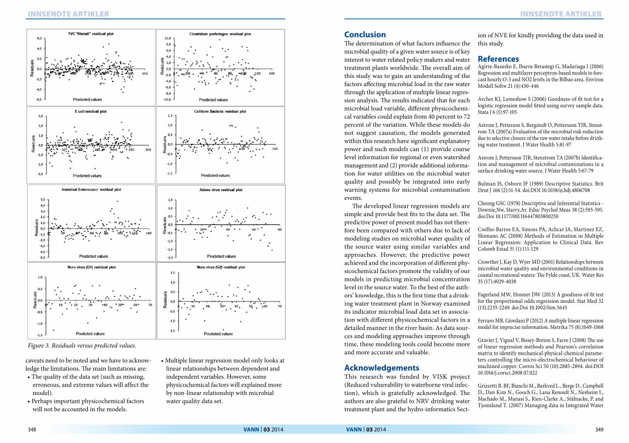
Finally, the residuals were plotted as a func-tion of the predicted values as illustrated in Figure 3. There is no obvious pattern in the resi-dual plots for any of the models. This means there is no left over information in the data that the models did not utilize. Moreover, it can be

seen from the plots that the residuals are distri-buted evenly above and below zero, which indi-cates that the variance is constant and does not depend on the predicted value. The models are therefore deemed valid for describing the depen-dent variables based on the selected explanatory data set.

Limitations of the StudyAlthough there is much remains to be done, our work generates important finding in the field of microbial water quality modelling using different physicochemical parameters. Even though this study generated important findings, a number of

Table 3. Regression coefficients.

Response Variable Predictors Coefficient Standard error t Pr > |t|

HPC

Constant -5,55 1,65 -3,37 0,0009

pH 1,01 0,27 3,75 0,0002

Conductivity 0,70 0,11 6,31 < 0,0001

Colour 0,06 0,01 10,11 < 0,0001

Clostridium perfringens

Constant -6,92 1,02 -6,81 <0,0001

pH 0,79 0,16 4,51 <0,0001

Temperature -0,04 0,01 -4,64 <0,0001

Conductivity 0,53 0,07 7,47 <0,0001

Colour 0,03 0,00 9,65 <0,0001

Escherichia coli

Constant -14,49 1,52 -9,52 <0,0001

Temperature -0,05 0,01 -4,88 < 0,0001

Turbidity -0,02 0,01 -2,57 0,0106

Conductivity 0,95 0,11 8,36 < 0,0001

Colour 0,04 0,00 8,35 <0,0001

pH 1,87 0,27 6,83 <0,0001

Coliform bacteria

Constant -14,76 1,29 -11,47 <0,0001

pH 2,23 0,20 11,33 <0,0001

Conductivity 0,64 0,07 8,84 < 0,0001

Colour 0,04 0,00 8,82 < 0,0001

Intestinal enterococci

Constant -2,43 0,56 -4,31 < 0,0001

Temperature -0,03 0,02 -1,95 0,043

Turbidity -0,03 0,01 -4,26 < 0,0001

Conductivity 0,98 0,12 8,35 < 0,0001

Colour 0,03 0,01 3,64 <0,0001

Adenovirus

Constant 12,03 4,32 2,79 0,007

pH -1,84 0,65 -2,83 0,006

Rainfall -0,13 0,04 -3,60 0,001

Conductivity 0,45 0,11 4,18 < 0,0001

Norovirus (GI)Constant 5,54 2,62 2,11 0,039

pH -1,02 0,35 -2,90 0,005

Conductivity 0,55 0,10 5,60 < 0,0001

Norovirus (GII)

Constant 0,05 0,77 0,06 0,953

Turbidity -0,33 0,07 -4,67 < 0,0001

Conductivity 0,42 0,13 3,23 0,002

Temperature -0,03 0,02 -1,93 0.049

Table 4. ANOVA for regression.

Response Variable Source DF Sum of squares Mean squares F Pr > F

HPC

Regression 3 315.62 78.90 71.08 < 0.0001

Residual 287 429.80 1.42

Total 290 745.42


Regression 4 1196.01 299.00 87.19 < 0.0001

Residual 286 1677.65 14.98

Total 290 2873.66

Escherichia coli

Regression 5 116.72 29.18 247.90 < 0.0001

Residual 293 112.64 0.46

Total 298 229.36

Coliform bacteria

Regression 3 15.08 5.03 142.30 < 0.0001

Residual 523 16.22 0.12

Total 526 31.29


Regression 4 110.89 27.72 22.07 < 0.0001

Residual 123 154.49 1.26

Total 127 265.37

Adenovirus

Regression 3 15.15 5.05 15.62 < 0.0001

Residual 70 22.63 0.32

Total 73 37.78

Norovirus (GI)

Regression 2 6.94 3.47 24,05 < 0.0001

Residual 60 8.65 0.14

Total 62 15.59

Norovirus (GII)

Regression 3 12.95 4.32 19.04 < 0.0001

Residual 55 12.47 0.23

Total 58 25.41

346 347 Vann I 03 2014 Vann I 03 2014


Table 5. VIF values for the multicollinearity test.

Response Variable Explanatory variables VIF

HPC

pH 1.766

Conductivity 1.788

Colour 1.176


pH 1.821

Temperature 1.035

Conductivity 1.959

Colour 1.648

Escherichia coli

Temperature 1.341

Turbidity 1.311

Conductivity 1.557

Colour 1.484

pH 1.034

Coliform bacteria

pH 1.019

Conductivity 3.316

Colour 1.066


Temperature 2,118

Turbidity 2,859

Conductivity 4,588

Colour 1,543

Adenovirus

pH 1,225

Rainfall 1,128

Conductivity 1,175

Norovirus (GI)pH 1,041

Conduct 1,041

Norovirus (GII)

Turbidity 1,235

Conductivity 1,592

Raw water temperature 1,743

Table 6. Goodness of fit statistics of the regression models.

Statistics HPC C.perfringens E coliColiform bacteria


AdenovirusNorovirus

(GI)Norovirus

(GII)

R² 0.42 0.55 0.72 0.45 0.42 0.40 0.45 0.51

Adjusted R² 0.41 0.54 0.71 0.45 0.40 0.38 0.43 0.48

MSE 1.42 14.98 0.46 0.12 1.26 0.32 0.14 0.23

RMSE 1.19 3.87 0.68 0.35 1.12 0.57 0.38 0.47

Figure 2. Microbial water quality variables predicted versus actual observation (95 % CI).

348 349 Vann I 03 2014 Vann I 03 2014


ConclusionThe determination of what factors influence the microbial quality of a given water source is of key interest to water related policy makers and water treatment plants worldwide. The overall aim of this study was to gain an understanding of the factors affecting microbial load in the raw water through the application of multiple linear regres-sion analysis. The results indicated that for each microbial load variable, different physicochemi-cal variables could explain from 40 percent to 72 percent of the variation. While these models do not suggest causation, the models generated within this research have significant explanatory power and such models can (1) provide coarse level information for regional or even watershed management and (2) provide additional informa-tion for water utilities on the microbial water quality and possibly be integrated into early warning systems for microbial contamination events.

The developed linear regression models are simple and provide best fits to the data set. The predictive power of present model has not there-fore been compared with others due to lack of modeling studies on microbial water quality of the source water using similar variables and approaches. However, the predictive power achieved and the incorporation of different phy-sicochemical factors promote the validity of our models in predicting microbial concentration level in the source water. To the best of the auth-ors’ knowledge, this is the first time that a drink-ing water treatment plant in Norway examined its indicator microbial load data set in associa-tion with different physicochemical factors in a detailed manner in the river basin. As data sour-ces and modeling approaches improve through time, these modeling tools could become more and more accurate and valuable.

acknowledgements This research was funded by VISK project (Reduced vulnerability to waterborne viral infec-tion), which is gratefully acknowledged. The authors are also grateful to NRV drinking water treatment plant and the hydro-informatics Sect-

ion of NVE for kindly providing the data used in this study.

ReferencesAgirre-Basurko E, Ibarra-Berastegi G, Madariaga I (2006) Regression and multilayer perceptron-based models to fore-cast hourly O-3 and NO2 levels in the Bilbao area. Environ Modell Softw 21 (4):430-446

Archer KJ, Lemeshow S (2006) Goodness-of-fit test for a logistic regression model fitted using survey sample data. Stata J 6 (1):97-105

Astrom J, Petterson S, Bergstedt O, Pettersson TJR, Stenst-rom TA (2007a) Evaluation of the microbial risk reduction due to selective closure of the raw water intake before drink-ing water treatment. J Water Health 5:81-97

Astrom J, Pettersson TJR, Stenstrom TA (2007b) Identifica-tion and management of microbial contaminations in a surface drinking water source. J Water Health 5:67-79

Bulman JS, Osborn JF (1989) Descriptive Statistics. Brit Dent J 166 (2):51-54. doi:DOI 10.1038/sj.bdj.4806708

Cheong GSC (1978) Descriptive and Inferential Statistics - Downie,Nw, Starry,Ar. Educ Psychol Meas 38 (2):593-595. doi:Doi 10.1177/001316447803800250

Coelho-Barros EA, Simoes PA, Achcar JA, Martinez EZ, Shimano AC (2008) Methods of Estimation in Multiple Linear Regression: Application to Clinical Data. Rev Colomb Estad 31 (1):111-129

Crowther J, Kay D, Wyer MD (2001) Relationships between microbial water quality and environmental conditions in coastal recreational waters: The Fylde coast, UK. Water Res 35 (17):4029-4038

Fagerland MW, Hosmer DW (2013) A goodness-of-fit test for the proportional odds regression model. Stat Med 32 (13):2235-2249. doi:Doi 10.1002/Sim.5645

Ferraro MB, Giordani P (2012) A multiple linear regression model for imprecise information. Metrika 75 (8):1049-1068

Gravier J, Vignal V, Bissey-Breton S, Farre J (2008) The use of linear regression methods and Pearson’s correlation matrix to identify mechanical-physical-chemical parame-ters controlling the micro-electrochemical behaviour of machined copper. Corros Sci 50 (10):2885-2894. doi:DOI 10.1016/j.corsci.2008.07.022

Grizzetti B. BF, Bianchi M., Barkved L., Berge D., Campbell D., Dan Kim N., Gooch G., Lana Renoult N., Nesheim I., Machado M., Manasi S., Rieu-Clarke A., Stålnacke, P. and Tjomsland T. (2007) Managing data in Integrated Water

Figure 3. Residuals versus predicted values.

caveats need to be noted and we have to acknow-ledge the limitations. The main limitations are:•Thequalityofthedataset(suchasmissing,

erroneous, and extreme values will affect the model).

•Perhapsimportantphysicochemicalfactorswill not be accounted in the models.

•Multiplelinearregressionmodelonlylooksatlinear relationships between dependent and independent variables. However, some physico chemical factors will explained more by non-linear relationship with microbial water quality data set.

350 Vann I 03 2014

Innsendte artIkler

Resources Management projects: the STRIVER case. Euro-pean Commission Joint Research Center. Institute for Envi-ronment and Sustainability. Rural, Water and Ecosystem Resources Unit (JRC-EC). doi:http://kvina.niva.no/striver/Portals/0/documents/STRIVER_D21.pdf

Han M, Zhao ZW, Cui FY, Gao W, Liu J, Zeng ZQ (2012) Pretreatment of contaminated raw water by a novel double-layer biological aerated filter for drinking water treatment. Desalin Water Treat 37 (1-3):308-314

Kinzelman J, McLellan SL, Daniels AD, Cashin S, Singh A, Gradus S, Bagley R (2004) Non-point source pollution: Determination of replication versus persistence of Esche-richia coli in surface water and sediments with correlation of levels to readily measurable environmental parameters. J Water Health 2 (2):103-114

Kovdienko NA, Polishchuk PG, Muratov EN, Artemenko AG, Kuz’min VE, Gorb L, Hill F, Leszczynski J (2010) Appli-cation of Random Forest and Multiple Linear Regression Techniques to QSPR Prediction of an Aqueous Solubility for Military Compounds. Mol Inform 29 (5):394-406

Kubeck C, van Berk W, Bergmann A (2009) Modelling raw water quality: development of a drinking water manage-ment tool. Water Sci Technol 59 (1):117-124

Kufs CT (1992) Statistical Modeling of Hydrogeologic Data.1. Regression and Anova Models. Ground Water Monit R 12 (2):120-130

Mills MS, Thurman EM (1994) Reduction of Nonpoint-Source Contamination of Surface-Water and Groundwater by Starch Encapsulation of Herbicides. Environ Sci Technol 28 (1):73-79

Mudelsee M (2003) Estimating Pearson’s correlation coef-ficient with bootstrap confidence interval from serially dependent time series. Math Geol 35 (6):651-665. doi:Doi 10.1023/B:Matg.0000002982.52104.02

Obrien PC, Shampo MA (1981) Descriptive Statistics.1. Mayo Clin Proc 56 (1):47-49

Pikkemaat GF (1969) Scope of Descriptive Statistics. Econ-omist 117 (3):258-275

Pugh EW, Papanicolaou GJ, Justice CM, Roy-Gagnon MH, Sorant AJM, Kingman A, Wilson AF (2001) Comparison of variance components, ANOVA and regression of offspring on midparent (ROMP) methods for SNP markers. Genet Epidemiol 21:S794-S799

Sedmak G, Bina D, MacDonald J, Couillard L (2005) Nine-year study of the occurrence of culturable viruses in source water for two drinking water treatment plants and the influ-ent and effluent of a wastewater treatment plant in Milwau-kee, Wisconsin (August 1994 through July 2003). Appl Environ Microb 71 (2):1042-1050

Ukoumunne OC, Gulliford MC, Chinn S (2002) A note on the use of the variance inflation factor for determining sample size in cluster randomized trials. J Roy Stat Soc D-Sta 51:479-484

Vounatsou P, Karydis M (1991) Environmental Characte-ristics in Oligotrophic Waters - Data Evaluation and Statis-tical Limitations in Water-Quality Studies. Environ Monit Assess 18 (3):211-220

Williams S (1996) Pearson’s correlation coefficient. New Zeal Med J 109 (1015):38-38

Won G, Kline TR, LeJeune JT (2013) Spatial-temporal varia-tions of microbial water quality in surface reservoirs and canals used for irrigation. Agr Water Manage 116:73-78

XLSTAT (2012) Running a partial least squares (PLS) discriminant analysis with XLSTAT-PLS. http://www.xlstat.com/en/learning-center/tutorials/running-a-partial-least-square-pls-discriminant-analysis-with-xlstat-pls.htm. Accessed May, 27 2014

Yang YP, Xue LG, Cheng WH (2011) The Empirical Likeli-hood Goodness-of-Fit Test for a Regression Model with Randomly Censored Data. Commun Stat Theory 40 (3):424-435. doi:Pii 929446357 Doi 10.1080/03610920903366156

Zhang Q, Stanley SJ (1997) Forecasting raw-water quality parameters for the North Saskatchewan River by neural network modeling. Water Res 31 (9):2340-2350

Multiple Linear Regression Models for Estimating Microbial … · Multiple Linear Regression Models...

Documents

Transcript of Multiple Linear Regression Models for Estimating Microbial … · Multiple Linear Regression Models...