Estimating Driver Performance Using Multiple

Electroencephalography (EEG)-Based Regression Algorithms

by Gregory Apker, Brent Lance, Scott Kerick, and Kaleb McDowell

ARL-TR-7074 September 2014 Approved for public release; distribution is unlimited.

NOTICES

Disclaimers The findings in this report are not to be construed as an official Department of the Army position unless so designated by other authorized documents. Citation of manufacturer’s or trade names does not constitute an official endorsement or approval of the use thereof. Destroy this report when it is no longer needed. Do not return it to the originator.

Army Research Laboratory Aberdeen Proving Ground, MD 21005-5425

ARL-TR-7074 September 2014

Estimating Driver Performance Using Multiple Electroencephalography (EEG)-Based Regression

Algorithms

Gregory Apker

School of Biological and Health Systems Engineering, Arizona State University

Brent Lance, Scott Kerick, and Kaleb McDowell Human Research and Engineering Directorate, ARL

Approved for public release; distribution is unlimited

ii

REPORT DOCUMENTATION PAGE Form Approved OMB No. 0704-0188

Public reporting burden for this collection of information is estimated to average 1 hour per response, including the time for reviewing instructions, searching existing data sources, gathering and maintaining the data needed, and completing and reviewing the collection information. Send comments regarding this burden estimate or any other aspect of this collection of information, including suggestions for reducing the burden, to Department of Defense, Washington Headquarters Services, Directorate for Information Operations and Reports (0704-0188), 1215 Jefferson Davis Highway, Suite 1204, Arlington, VA 22202-4302. Respondents should be aware that notwithstanding any other provision of law, no person shall be subject to any penalty for failing to comply with a collection of information if it does not display a currently valid OMB control number. PLEASE DO NOT RETURN YOUR FORM TO THE ABOVE ADDRESS. 1. REPORT DATE (DD-MM-YYYY)

September 2014 2. REPORT TYPE

Final 3. DATES COVERED (From - To)

May 2012–September 2013 4. TITLE AND SUBTITLE

Estimating Driver Performance Using Multiple Electroencephalography (EEG)-Based Regression Algorithms

5a. CONTRACT NUMBER

5b. GRANT NUMBER

5c. PROGRAM ELEMENT NUMBER

6. AUTHOR(S)

Gregory Apker, Brent Lance, Scott Kerick, and Kaleb McDowell

5d. PROJECT NUMBER

5e. TASK NUMBER

5f. WORK UNIT NUMBER

7. PERFORMING ORGANIZATION NAME(S) AND ADDRESS(ES)

US Army Research Laboratory ATTN: RDRL-HRS-C Aberdeen Proving Ground, MD 21005-5425

8. PERFORMING ORGANIZATION REPORT NUMBER

ARL-TR-7074

9. SPONSORING/MONITORING AGENCY NAME(S) AND ADDRESS(ES)

10. SPONSOR/MONITOR’S ACRONYM(S) 11. SPONSOR/MONITOR'S REPORT NUMBER(S)

12. DISTRIBUTION/AVAILABILITY STATEMENT

Approved for public release; distribution is unlimited. 13. SUPPLEMENTARY NOTES

14. ABSTRACT

Poor driving caused by fatigue and drowsiness is the cause of many car accidents each year despite a number of vehicle-mounted sensors designed to infer driver state from behavior. Recent research into the neural correlates of fatigue has suggested the potential for the use of electroencephalographic (EEG) signals to not only detect the fatigue onset in drivers, but also predict the corresponding drop in performance. Here, we sought to compare the performance of 3 EEG regression approaches (linear principal component [PC], linear support vector regression [SVR], and radial basis function SVR) designed to provide continuous estimates of driver error during an extended simulated driving session. Eleven subjects were asked to maintain the heading and speed of their vehicle during 45 min of simulated driving, with average deviation from the center of the cruising lane used as the measure of driver error. Lane deviation and 64-channel EEG data were recorded during the session and processed offline, and 10-fold cross validation was used to assess model performance. In general, all 3 approaches produced significantly correlated estimates of driver error; however, the correlation coefficients varied significantly between cross-validation blocks, potentially because of inter-block variability in the measure of driver error. Prediction errors of both SVR-based models were significantly smaller than those of the PC-based model, but no difference was found between SVR-based approaches. These results indicate that regression models can be used to extract continuous information of driver performance; however, the variability in correlation analysis suggests that lane deviation may not be an ideal measure of driver performance, and that regression performance may improve from a more stable metric of driver performance as simulated driving complexity increases. 15. SUBJECT TERMS

EEG, fatigue, regression, SVR, electroencephalography, PC

16. SECURITY CLASSIFICATION OF: 17. LIMITATION OF ABSTRACT

UU

18. NUMBER OF PAGES

28

19a. NAME OF RESPONSIBLE PERSON Scott Kerick

a. REPORT

Unclassified b. ABSTRACT

Unclassified c. THIS PAGE

Unclassified 19b. TELEPHONE NUMBER (Include area code) 410-278-5833

Standard Form 298 (Rev. 8/98) Prescribed by ANSI Std. Z39.18

iii

Contents

List of Figures iv

List of Tables iv

1. Introduction 1

2. Experimental Setup 3

2.1 Subjects ...........................................................................................................................3

2.2 Driving Simulation ..........................................................................................................3

2.3 Data Collection and Analysis ..........................................................................................4 2.3.1 Vehicle Status and Performance Metrics ............................................................5 2.3.2 Electroencephalography ......................................................................................5

3. Performance Prediction 5

3.1 Cross-Validation Preparation ..........................................................................................5

3.2 PC-Based Regression ......................................................................................................6

3.3 Support Vector Regression ..............................................................................................6

3.4 Statistical Analysis ..........................................................................................................7

4. Results 7

4.1 Driver Performance .........................................................................................................7

4.2 Correlation of Driver Error and EEG ..............................................................................8

4.3 PC-Based Prediction Accuracy .......................................................................................8

4.4 SVR-Based Prediction Accuracy ..................................................................................10 4.4.1 Linear SVR ........................................................................................................10 4.4.2 Nonlinear SVR ..................................................................................................11

4.5 Model Comparison ........................................................................................................13

5. Discussion and Conclusions 14

6. References 18

Distribution List 21

iv

List of Figures

Fig. 1 Driving simulation and processing and regression for driver performance prediction. A) Driving simulator apparatus. B) Calculation of lane deviation for driver error quantification. C) Processing steps of 64-channel EEG data for regression models and diagram of “Modeling and Estimation of Driver Error” step of Fig. 1C for the PC-based and SVR-based model. Eigenvectors and model coefficients were calculated from data in the training cross-validation (CV) blocks and applied to data from the testing block. .............4

Fig. 2 Driver error values from 6 representative subjects. Some subjects maintained consistent control around a baseline offset throughout the 45-min drive (drivers A, D, F) while others exhibited periods of increased variability (drivers B, C, E). .................................6

Fig. 3 Prediction of driver error from the PC-based algorithm for 2 subjects. Actual (black lines) and estimated (blue lines) values of driver error for 2 subjects. Vertical red lines delineate CV blocks. ..................................................................................................................8

Fig. 4 Estimation of driver error from the SVR-based algorithm for 2 subjects. Average actual (black lines) and SVR-based prediction (blue lines) lane deviations for the same subjects shown in Fig. 3. Vertical red lines delineate CV blocks. ...........................................10

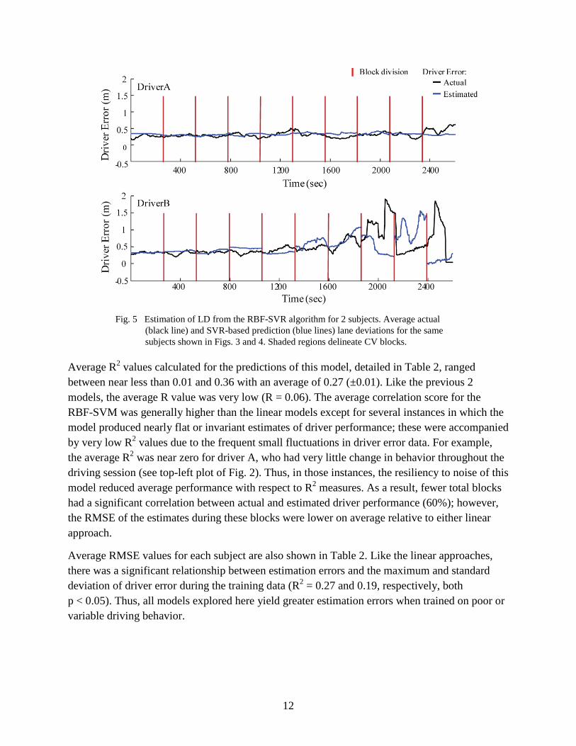
Fig. 5 Estimation of LD from the RBF-SVR algorithm for 2 subjects. Average actual (black line) and SVR-based prediction (blue lines) lane deviations for the same subjects shown in Figs. 3 and 4. Shaded regions delineate CV blocks. ............................................................12

Fig. 6 Comparison of (A) RMSE and (B) R2 between PC- and SVR-based predictions. Left-hand side box plots indicate the ratios of average RMSE (A) and R2 (B) for each subject between 3 models. ....................................................................................................................14

List of Tables

Table 1 Maximum and the standard deviation of the smoothed driver error across the entire driving session for each subject. ................................................................................................8

Table 2 Average squared correlation coefficient and corrected MSE of predicted driver error across cross-validation blocks for each subject for the 3 driver error models ...........................9

1

1. Introduction

Fatigue is a pervasive problem among drivers, estimated to have contributed to between 35% and 40% of all accidents and costing in excess of $375 billion annually worldwide (Fletcher et al. 2005, Treat et al. 1977). To reduce these effects, many systems have been designed to detect driver fatigue before it affects driver performance. Typically, these systems have relied on vehicle-mounted sensors to monitor driver behaviors associated with fatigue, such as posture or eye-blinking characteristics (Perez et al. 2001, Popieul et al. 2003, Smith et al. 2000). However, several researchers have argued that monitoring the neural correlates of fatigue using electroencephalography (EEG) may provide a more reliable estimate of driver fatigue (Lal and Craig 2002, Okogbaa et al. 1994). An advantage of this approach is that it would detect signals that are ostensibly more directly related to the physiological effects of fatigue rather than behaviors that are only circumstantially related to fatigue.

The findings have led to the development of several classification algorithms designed to detect the onset of fatigue in drivers from neural signals alone. These algorithms employ a wide variety of classification approaches to detect the onset of fatigue, ranging from Bayesian inference to neural networks (Peiris et al. 2011, Sandberg et al. 2011, Stikic et al. 2011, Yang et al. 2012, Zhao et al. 2011). The success of these systems suggests a fairly robust relationship between neural signals and driver fatigue. However, the predictions of these classification algorithms typically involve computationally intensive processing steps, limiting their application to largely offline analysis. Thus, these algorithms are not well situated to be embedded in a real-time system for fatigue detection.

In addition, these classification methods typically do not attempt to make the connection between the levels of fatigue they detect and their influence on behavior. In a line of recent work, Lin and colleagues have demonstrated a strong linear relationship between EEG-based signals and fluctuations in driver performance associated with fatigue (Chuang et al. 2012, Lin et al. 2005a, 2005b, Lin et al. 2006, Makeig and Jung 1995). This relationship was demonstrated using a variety of behaviors and processing techniques, one of the most intriguing of which was based upon a strong linear correlation found between power-spectral estimates and vehicle lane deviation. Using only basic signal processing and linear regression, the researchers developed an EEG-based driver performance estimation algorithm that yielded accurate predictions with relatively minimal processing (Lin et al. 2005a).

As argued by the authors, the simplicity and accuracy of their approach make this model attractive for translation to a real-time system for estimating driver performance. Because the model makes few a priori assumptions about the connection between brain signals and driver performance, it is possible that the model is not necessarily sensitive to fatigue but rather adapts to the subject’s specific patterns of behavior and neural activity. In this way, it is possible that

2

this technique may extend beyond the context of driving or fatigue to be a generalizable approach to predict changes in performance from brain behavior. Additionally, it is possible that the method is capable of generalizing across a broader array of drivers and to more sensitive measures of driving performance. However, this method has been evaluated against only a simplistic driving model in which vehicle movement and control were highly constrained, and all drivers exhibited significant behavioral changes due to drowsiness. To assess whether this approach can generalize to real-world systems of this approach, it is important to first establish how well it generalizes across a broader sample of driver/driving behavior.

Another challenge of transitioning EEG-based driver prediction technologies from laboratory simulations to real-world driving is that changes in task dynamics (such as those associated with more natural driving conditions) can have significant effects on the neural activity associated with fatigue and task performance (Desmond and Mathews 1997, 2002, Pattyn et al. 2008). As a result, the diverse physiological effects of drowsiness and the unpredictable effects of more naturalistic tasks raise concern of whether a simple linear model can adequately represent the relationship between neural signals and driving performance. As a result, more naturalistic driving tasks may require more sophisticated algorithms capable of distinguishing relevant signals amidst noisy input. One such approach comes from the field of machine learning, where kernel-based methods, such as support vector machine (SVM) algorithms, have been successfully employed in fatigue detection systems and have been shown to provide more robust performance despite noisy input features (Shen et al. 2007, Shen et al. 2008). Support vector regression (SVR), a variant of SVMs, offers similar advantages as SVMs and can be trained to directly estimate driver performance similar to the method described in Lin et al. (2005a) to provide a higher-resolution estimate of driver fatigue than previous SVM-based classifiers (Drucker et al. 1997).

To evaluate the generalization of linear models for driver performance estimation across individuals and potential translation to more realistic driving, we adapted an established linear regression method as well as SVR-based approaches to estimate driver performance during a simulated driving task in which subjects must rigorously control the speed and heading of a vehicle with realistic dynamics. Subjects completed 45 min of continuous driving in which they were required to maintain vehicle speed and heading, and react to intermittent lateral perturbations to the vehicle. Models were trained to predict driver performance from the simultaneously recorded EEG data. All algorithms yielded low but significant levels of correlation with actual driving performance more than 70% of the time, suggesting that this approach can capture information related to fluctuations of driver performance in more complex driving tasks but may be improved by a more stable metric of performance than lateral deviation of the vehicle.

3

2. Experimental Setup

2.1 Subjects

Eleven subjects (20 to 40 years old) participated in a simulated highway driving experiment. Each subject was briefed on the experimental equipment and procedures, and signed an informed consent form. The voluntary, fully informed consent of the persons used in this research was obtained as required by Title 32 Part 219 of the Code of Federal Regulations (2013) and Army Regulations 70–25 (1990) and approved as project No. ARL 10-051. The investigators adhered to the policies for the protection of human subjects as prescribed in Army Regulation 70–25 (1990). No constraints were placed on the subjects related to previous night’s sleep or diet, nor were subjects required to complete the experiment at a specific time of day.

2.2 Driving Simulation

Subjects completed 2 separate driving sessions: an acclimation session (15 min) and an experimental session (45 min). Before each session, subjects provided an estimate of their fatigue level via the Karolinska Sleepiness Scale (Akerstedt and Gillberg 1990). Additionally, subjects were asked to verbally report their fatigue score on this scale every 15 min during the experimental session without interruption of driving.

Subjects drove down a straight, infinitely long highway (Fig. 1A) and were instructed to keep their vehicle as close to the center of the right-hand lane as possible. Throughout the session, after subjects had maintained the vehicle within the appropriate lane for 8–10 s, a lateral perturbation was applied to the vehicle, causing it to begin to veer off course. The strength of the perturbation increased until the driver made a corrective steering adjustment (defined as a steering wheel deflection of 4° in the opposite direction of the perturbation) at which point the perturbation ceased, allowing the subject to return the vehicle to the center of the driving lane. The perturbation would ramp down automatically after approximately 3 s if no correction was made; however, the driver was still required to correct the vehicle’s heading and position. If the subject did not perform a corrective steering adjustment, the vehicle would continue to veer out of the lane and off the road until it was 21.9 m outside of the lane. At this point, the driver would be alerted to regain control of the vehicle via an auditory cue.

In addition to maintaining control of the vehicle’s direction, drivers also maintained appropriate speed during the testing session via accelerator and brake pedals. Subjects were instructed to obey posted speed limit signs, which appeared on the right-hand side of the road during the driving session. The speed limit was 45 mph for most of the session; however, at 3 different points during the 45-min driving session, the posted speed limit was reduced to 25 mph.

4

Fig. 1 Driving simulation and processing and regression for driver performance prediction. A) Driving simulator apparatus. B) Calculation of lane deviation for driver error quantification. C) Processing steps of 64-channel EEG data for regression models and diagram of “Modeling and Estimation of Driver Error” step of Fig. 1C for the PC-based and SVR-based model. Eigenvectors and model coefficients were calculated from data in the training cross-validation (CV) blocks and applied to data from the testing block.

2.3 Data Collection and Analysis

Vehicle position and EEG were collected simultaneously throughout the experiment. Eye position was also monitored but not analyzed here. Specific event markers were embedded within each data structure and used to align the data in time and remove any drift in the time series of each data stream.

5

2.3.1 Vehicle Status and Performance Metrics

Vehicle status (position and dynamics) was monitored throughout each session, sampled at 90 Hz for subjects 1–7 and at 100 Hz for subjects 8–11. To estimate driver performance, the vehicle’s lateral deviation was calculated for the entire session as the difference between the center of the vehicle and the center of the cruising lane (Fig. 1B). To account for the tendencies of some subjects to consistently position the vehicle to the right or left of the center of the lane, the median of their offset was subtracted. Lane deviation was then calculated as the absolute value of the lateral deviation throughout the driving session, then smoothed using a 90-s moving average filter with a 2-s step size as fluctuations in fatigue and alertness tend to last between 1 and 2 min (Makeig and Jung 1995). This smoothed measure represents the driver’s average ability to maintain control of the vehicle, and thus the smoothed estimates of lane deviation act as our measure of driver error.

2.3.2 Electroencephalography

EEG signals were collected using a 64-channel Biosemi EEG system, sampled at 2048 Hz and down-sampled to 256 Hz off-line. The power spectral density (PSD) estimates for each channel were calculated using a 750-point Hanning window with a 250-point overlap. Each channel and frequency power estimate was then smoothed with the same 90-s moving average filter used to smooth the lane deviation data. Effects of fatigue have typically been shown to affect PSD estimates as low as the theta band (4–8 Hz). Thus, to reduce the influence of the large power fluctuations inherent to the EEG signal below the theta range, we used a frequency range between 5 and 50 Hz for subsequent analyses. As described in Lin et al. (2005a), correlation between PSD estimates and driver error were often strongest for channels Cz and Pz, and as such, these 2 channels were selected for subsequent processing.

3. Performance Prediction

3.1 Cross-Validation Preparation

To allow driving behavior to stabilize, we removed the first 100 s of smoothed driving data (10 s to move to the center of the cruising lane, plus 90 s due to smoothing). Following this, the aligned EEG and vehicle data from the experimental session were split into 10 equal blocks to train and test each prediction approach. Ten-fold cross-validation (CV) was conducted such that 9 blocks were used to train the prediction algorithm, and the remaining block was used to assess prediction performance. To eliminate overlapping data between training and testing sets, 90 s of the training data that abutted the testing data was removed prior to each CV block.

6

3.2 PC-Based Regression

Principal component analysis (PCA) was performed on the combined PSD estimates of both Cz and Pz from the training data. Using these eigenvectors, we projected both training and testing PSD estimates into the component space, and only the top 50 principal components (PCs) based on their eigenvalues were reserved to reduce the dimensionality of the feature space.

The projected PSD data from the training blocks were used to calculate the coefficients of a 51-parameter (50 component vectors plus a column of ones to account for bias/offset) linear regression model of lane deviation. These regression coefficients were then applied to the projected PSD estimates of the testing block to generate a prediction of driver error over this period (Fig. 2). These predictions were compared to the measured driver performance for each epoch to characterize the predictive accuracy of the approach. This was repeated separately for each CV block, providing 10 unique estimates of model performance for each subject.

Fig. 2 Driver error values from 6 representative subjects. Some subjects maintained consistent control around a baseline offset throughout the 45-min drive (drivers A, D, F) while others exhibited periods of increased variability (drivers B, C, E).

3.3 Support Vector Regression

SVM algorithms, a form of machine learning algorithm, are commonly used in EEG-based fatigue detection because they offer additional optimization criteria that can yield more robust performance in stochastic systems. SVR is an adaptation of an SVM, which approximates functions used for direct estimation of a parameter (Drucker et al. 1997). In this study, the LIBSVM library was used to develop the SVR model and generate the predictions of driving behavior (Chang and Lin 2011). A linear kernel function was used to provide another means of evaluating the potential of using linear regression to predict driver performance. Recent work has shown encouraging results classifying fatigue onset using a radial basis function (RBF) kernel in

7

SVM-based fatigue detection (Shen et al. 2007, 2008). Thus, we trained and tested an additional SVR-based model using a nonlinear RBF kernel to assess whether more complex driving scenarios instigate a more complex relationship between PSD estimates and driving performance. As shown in Fig. 2, feature inputs to each SVR were treated the same as those of the PC-based regression up to the point of PCA analysis. Thus, the smoothed PSD estimates for Cz and Pz channels were combined to generate driving performance predictions using the 2 SVR-based approaches.

3.4 Statistical Analysis

To compare algorithm performance between models, we calculated Pearson’s correlation coefficients between predicted and actual driver error within each CV block, as well as the bias-corrected root mean squared error (RMSE) of the prediction for each CV block. The PC- and SVR-based approaches were compared using a paired Wilcoxon sign rank test of model performance metrics, unless otherwise stated. P-values at or below 0.05 constituted the threshold of significance.

4. Results

4.1 Driver Performance

During the driving session, drivers maintained the appropriate speed indicated by the posted speed limit signs within 2–3 mph. Most of the session was spent maintaining a speed around 45 mph, and most drivers were quick to adjust when the speed limit dropped briefly to 25 mph and rose back to 45 mph. Driver error did not significantly vary between periods of fast and slow driving. As a result, driver error values during the entire driving session were used for regression and estimation analysis.

Driving performance varied greatly between subjects; some subjects maintained a high level of driving performance, whereas others exhibited periods of large or fluctuating performance. This difference is illustrated in Fig. 2, in which 3 subjects (drivers A, D, F) maintained relatively consistent vigilant driving performance, while other subjects exhibited predominantly vigilant (low error) driving but with a period of poor performance near the end of the session (drivers B, E), and still others produced large driving errors throughout the session (driver C). Such broad discrepancies were observed across all subjects as represented by the data in Table 1, which summarizes the maximum and standard deviation of the smoothed driver error across the entire experiment for all subjects. For instance, smoothed driver error in 3 of the 11 drivers did not exceed 0.5 m, whereas 3 other drivers produced average driver error values of 1.5 m over the 90-s window. Additionally, in some cases, large fluctuations in driver error were attributable to isolated periods of very poor driving, while some drivers produced generally more variable driver error values across the entire experiment. Thus, the driver population sampled here represents a wide range of driving behavior.

8

Table 1 Maximum and the standard deviation of the smoothed driver error across the entire driving session for each subject.

Meas. A (m)

B (m)

C (m)

D (m)

E (m)

F (m)

G (m)

H (m)

I (m)

J (m)

L (m) Average

Median 0.28 0.37 0.24 0.68 0.23 0.26 0.24 0.24 0.36 0.35 0.21 0.31 (±0.1) Max. 0.61 1.89 0.33 2.45 0.42 0.56 0.35 1.46 0.66 0.85 0.45 0.91 (±0.7)

St. Dev. 0.08 0.35 0.03 0.46 0.07 0.07 0.04 0.26 0.11 0.16 0.05 0.15 (±0.2)

4.2 Correlation of Driver Error and EEG

The correlation between driver error and PSD estimates across all 64 EEG channels also varied widely. Consistent with previous findings, the highest correlation values were typically found between 5 and 15 Hz; however, some subjects also had an increase in R2 at higher frequencies (25+ Hz) (Lin et al. 2005a). Also consistent with these earlier findings, channels Cz and Pz typically yielded among the highest average correlation; thus, these 2 channels were selected for subsequent regression analysis presented here for all subjects.

4.3 PC-Based Prediction Accuracy

Prediction accuracy of lane deviation for the PC-based model varied considerably between drivers and between CV blocks within a single driver. Figure 3 illustrates the predicted and actual driver error for 2 representative subjects across all 10 CVs represented. Model performance for driver A, who generally produced consistently good driving behavior, was reasonably accurate for most blocks, while in others, model performance was poorer. For the less consistent driver B, model errors were very large for all blocks, and model correlation performance varied between blocks.

Fig. 3 Prediction of driver error from the PC-based algorithm for 2 subjects. Actual (black

lines) and estimated (blue lines) values of driver error for 2 subjects. Vertical red lines delineate CV blocks.

9

The average coefficient of determination was R2 = 0.23 (±0.004), but the correlation coefficient between predicted and actual driver error across all subjects and blocks was only R = 0.031, indicating that large negative correlations were also common. Table 2 summarizes the average R2 values, explaining the variance accounted for by the model between the predicted and actual driver error for the PC-based model across all blocks for each subject. In general, average R2

values were similar between all subjects, ranging between 0.16 and 0.31. While these values are relatively low, across all subjects and all CV blocks, 9 of the 11 subjects tested exhibited at least one block with an R2 greater than 0.5. These are encouraging results given the more realistic driving simulation and ecologically valid subject pool to which the simple linear regression algorithm was applied.

Table 2 Average squared correlation coefficient and corrected MSE of predicted driver error across cross-validation blocks for each subject for the 3 driver error models

Subject PCA SVR Linear SVR RBF

RMSE (m)

R2

(m) RMSE

(m) R2

(m) RMSE

(m) R2

(m) A 0.01 0.21 0.01 0.24 0.02 0.19 B 0.22 0.23 0.14 0.21 0.22 0.23 C <0.0 0.3 <0.0 0 <0.0 <0.0 D 0.37 0.16 0.15 0.2 0.18 0.28 E 0.01 0.2 <0.0 0.23 <0.0 0.37 F 0.01 0.29 0.01 0.33 0.01 0.29 G 0.01 0.27 <0.0 0.22 <0.0 0.29 H 0.1 0.17 0.06 0.37 0.05 0.32 J 0.02 0.21 0.02 0.32 0.03 0.25 K 0.07 0.31 0.01 0.33 0.03 0.34 L 0 0.18 <0.0 0.18 <0.0 0.36

Mean 0.07 0.23 0.04 0.24 0.05 0.27

SD 0.12 0.05 0.06 0.1 0.08 0.1 Note: PCA = principal component analysis; SVR = support vector regression; RBF = radial basis function; and RMSE = root mean squared error.

10

Prediction errors varied widely between subjects and CV blocks. Table 2 also summarizes the average RMSE of the predicted driver error across all blocks for each subject for the PC-based model. In general, the algorithm produced smaller errors for subjects who exhibited more stable driving throughout the session (low maximum and standard deviation of driver error). This is particularly evident when compared to the errors produced for subject 3 who performed consistently well throughout the session and those for subject 4 who exhibited relatively large and more variable driving behavior.

A significant correlation was also found between the maximum and standard deviation of the driver error of the training data and RMSE of the estimates of the testing data (R2 = 0.38 and 0.30, respectively, p < 0.05 for both). This correlation suggests that the PC-based model predictions have trouble matching the larger fluctuations in driving performance, potentially because of relative infrequency of this behavior in the training sets. Interestingly, no correlation was found between these characteristics of the testing data and the R2 value of the prediction.

4.4 SVR-Based Prediction Accuracy

4.4.1 Linear SVR

Like the PC-based model, prediction accuracy of the SVR-based linear model varied considerably between drivers and between CV blocks within a driver. Figure 4 illustrates the predicted and actual driver error with all 10 CV blocks for the same subjects depicted in Fig. 3. The general trends in performance of the linear SVR-based model were very similar to those of the PC-based model in that prediction accuracy varied between blocks for both drivers, with prediction errors being consistently large for the more variable driving behavior.

Fig. 4 Estimation of driver error from the SVR-based algorithm for 2 subjects. Average actual (black lines) and SVR-based prediction (blue lines) lane deviations for the same subjects shown in Fig. 3. Vertical red lines delineate CV blocks.

11

This performance was consistent with the results of correlation analysis which revealed that average R2 values ranging between less than 0.01 and 0.37 across subjects with a population average of 0.24 (±0.007). However, like the PC-based model, the average R value was near zero (–0.01). Table 2 summarizes the average of the R2 for the linear SVR-based predictions of driver error across all blocks for each subject. These values are slightly larger than those of the PC-based model, with the exception of subject 3, for whom the SVR-based model could not fit a line, and thus predicted only a flat line for all 10 CV blocks. Nonetheless, for this approach significant prediction correlations were found for 80 of 110 instances (73%).

Like the correlation coefficients, RMSE values varied between subjects and blocks. Table 2 also summarizes the average RMSE of the predicted driver error across all blocks for each subject for the linear SVR-based model and shows highly subject-dependent prediction errors. A significant correlation was found between RMSE and the maximum and standard deviation of driver error in the training data (R2 = 0.42 and 0.36, respectively, with p < 0.001 for both), but this was a much stronger correlation than that of the PC-based model. Like the PC model, no correlation was found between these characteristics of the testing data and the R2 value of the prediction. This suggests that the predictions of the SVR-based model tended to be more accurate when variability of the training data is lower relative to estimates that were produced when periods of poor driving appeared in the training set.

4.4.2 Nonlinear SVR

The accuracy of the RBF-SVR model predictions again varied between subjects and often within each driving session. Figure 5 illustrates the predicted and actual driver error with all 10 CV blocks for the same subjects depicted previously. The RBF-SVR model produced flat (or nearly flat) line estimates of driver error. These blocks tended to be those in which there was little change in driver performance, such as those seen in several blocks of the top plot in Fig. 5 as well as in the first several blocks in the bottom plot of the figure. In other cases, the RBF model produced a generally straight line; however, the prediction matched the general trend of the actual behavior (e.g., blocks 6 and 7 of the bottom plot of Fig. 5). This suggests that the RBF-SVR-based model may be a little more resilient to noise and variability in the EEG or driver performance training data, which may be responsible for the large fluctuations in estimates of the 2 linear models.

12

Fig. 5 Estimation of LD from the RBF-SVR algorithm for 2 subjects. Average actual

(black line) and SVR-based prediction (blue lines) lane deviations for the same subjects shown in Figs. 3 and 4. Shaded regions delineate CV blocks.

Average R2 values calculated for the predictions of this model, detailed in Table 2, ranged between near less than 0.01 and 0.36 with an average of 0.27 (±0.01). Like the previous 2 models, the average R value was very low (R = 0.06). The average correlation score for the RBF-SVM was generally higher than the linear models except for several instances in which the model produced nearly flat or invariant estimates of driver performance; these were accompanied by very low R2 values due to the frequent small fluctuations in driver error data. For example, the average R2 was near zero for driver A, who had very little change in behavior throughout the driving session (see top-left plot of Fig. 2). Thus, in those instances, the resiliency to noise of this model reduced average performance with respect to R2 measures. As a result, fewer total blocks had a significant correlation between actual and estimated driver performance (60%); however, the RMSE of the estimates during these blocks were lower on average relative to either linear approach.

Average RMSE values for each subject are also shown in Table 2. Like the linear approaches, there was a significant relationship between estimation errors and the maximum and standard deviation of driver error during the training data (R2 = 0.27 and 0.19, respectively, both p < 0.05). Thus, all models explored here yield greater estimation errors when trained on poor or variable driving behavior.

13

4.5 Model Comparison

A significant difference was observed between RMSE values of the PC-based model and both SVR-based approaches. Figure 6A presents a comparison of estimation errors between the models. The box plot (top) illustrates the ratios of the average estimation error for each subject using the PC-based model to the 2 SVR-based approaches, as well as that of the linear SVR to the RBF SVR. Ratios greater than 1 indicate that the numerator was greater than the denominator. The median ratios of the PC-based model to linear SVR and RBF SVR were 1.15 and 1.19, respectively. A Wilcoxon test confirmed that these ratios were statistically greater than 1 (equivalence). Thus, on average, the PC-based model produced significantly greater estimation errors. The median ratio between the linear to RBF SVR was 1.00 and was not found to be different than 1, suggesting relatively similar average levels of estimation error. These results suggest that periods of driving that proved difficult for one model were also problematic for the others.

Despite PC-based predictions being significantly correlated with actual driver error more often than the SVR-based predictions (81% for the PC-based model versus 73% and 60% for the linear and RBF SVRs, respectively), the R2 values themselves were not significantly different between models across the population. Figure 6B illustrates the comparison between R2 values for the 3 models. The plot compares the ratio of the average R2 values for each subject between models. In all cases, the distributions of R2 ratios were generally centered around 1 (equivalence), and none of these distributions was found to be significantly different from 1 (paired Wilcoxon test), suggesting that the overall ability to model the fluctuations in driving performance was largely equal across the models. These results suggest that the basis of performance on a given block was likely driven by the nature of the relationship between the neural signals and driving performance rather than characteristics specific to the regression methodology.

14

Fig. 6 Comparison of (A) RMSE and (B) R2 between PC- and SVR-based predictions. Left-hand side box plots indicate the ratios of average RMSE (A) and R2 (B) for each subject between 3 models.

5. Discussion and Conclusions

We have evaluated 2 approaches to using linear regression models with PSD estimates to predict performance in a simulated driving task. Performance of both PC- and SVR-based models varied between and within subjects but was generally similar between models for a given subject and block. Overall, the average prediction errors of the SVR-based model for each subject were slightly but significantly smaller than those of the PC-based algorithm, but the PC-based algorithm yielded significant correlations to actual behavior more often. However, the accuracy of these predictions fell considerably short of previous driver prediction algorithms in simpler driving tasks (Lin et al. 2005a). Nonetheless, the frequent significant correlations suggest that linear regression models of PSD estimates can provide some insight into driver performance even as the vehicle simulation becomes more realistic (i.e., requiring constant speed and heading control).

15

In a 2005 study, Lin et al. showed strong linear relationship between lane deviation EEG recordings from 2 channels in a simple driving scenario (2005a). Using a very similar PC-based method, as well as an alternative SVR-based approach, we were unable to produce the same level of correlation in a more complex driving task. This may be due to at least several factors associated with our translational approach. First, in the Lin et al. study, the application of the driving performance model was limited to only those drivers who showed multiple instances of drowsiness and microsleeps as validated from video recordings. This reduced their driver population from 16 to 5 candidate drivers who were most likely to exhibit poor driving behavior due solely to driver fatigue (Lin et al. 2005a). Second, in contrast to this initial study, in the present study drivers had to maintain continuous control of both heading and speed during the entire experiment, adding another element of task complexity that may have had an unpredictable effect on the patterns of neural activity (Desmond and Matthews 1997, Desmond and Matthews 2002, Pattyn et al. 2008).

Another factor potentially contributing to lower correlations is the fact that the realistic steering and vehicle dynamics introduced greater variance or prolonged changes in lane deviation not necessarily due to a lack of attention or fatigue or without a consistent neural basis. In fact, in more recent work, Lin and colleagues have focused on the relationship between neural activity and driver reaction time rather than lane deviation (Chuang et al. 2012). Both of these factors may introduce potentially confounding influences into the behavioral and/or neural data. Thus, future developments of driver prediction technologies may entail evaluating other metrics of driver performance that will be more reflective of the driver state, isolated from the factors related to the vehicle or outside world.

The SVR-based approaches were explored as a means to evaluate whether a more complex algorithm would be more robust to variability in the feature (e.g., PSD estimates) and target (driver error calculated from lane deviation) spaces introduced by a naturalistic driving task. Interestingly, while both SVR-based models yielded significantly lower prediction errors relative to the PC-based model, neither was better able to approximate the relationship between PSD estimates and behavior. However, as task conditions continue to become more complex, the added accuracy of the SVR-based approach may prove to be worth the added computational load. Further, in case of driver A, it is evident that the RBF-SVR-based approach was less likely to fit a model when there is relatively little change in driver performance relative to minor fluctuations (noise) in vehicle position. While this ostensibly hurt the performance of the model here, this characteristic may be advantageous as driving scenarios become more complex, resulting in more variability in the performance metric.

16

For all 3 regression approaches, we observed very large discrepancies between the correlations observed during model training and testing, which is a characteristic of overfitting. It is common for fatigue detection systems to average power across several frequencies to focus on specific bands, such as theta (5–8 Hz) and alpha (8–12 Hz), given their known relationship with fatigue onset (for a review, see Lal and Craig 2001). This approach yields a much smaller feature space, which can lead to a more robust fit; however, the advantage of a high-dimensional regression model is the potential to provide a higher-resolution prediction of driver performance. Thus, compression of PSD features into broad frequency bands (or outright rejections of some) could sacrifice useful information regarding changes in driver performance. One possible method to minimize the potential for overfitting and preserve predictive resolution is to employ step-wise regression during model formulation, a process shown to be effective in the detection of fatigue from PSD estimates (Sticik et al. 2011).

A hallmark of the EEG data processing preformed here is its relative simplicity to preserve computational speed in potential real-time systems. However, it is worth noting that despite the success of the simple algorithm employed in Lin et al. (2005a), subsequent studies from this group have used additional processing steps, such as fuzzy neural networks and independent component analysis to link driving behavior and EEG data (Chuang et al. 2012, Lin et al. 2005b, Lin et al. 2006). These techniques can significantly influence the effect of noise and/or artifacts in the neural features but are considerably more computationally and time intensive and are limited to post-hoc analysis and/or cannot be continually updated in real time. As algorithms and processers become more efficient, such techniques may prove an important modification to enhance the regression algorithms evaluated here.

Characteristic of all 3 regression approaches evaluated here, performance varied between CV blocks, performing very well in some and poorly in others. This behavior represents a significant challenge to the translation of EEG-based driver performance estimation technologies, particularly those that rely on a linear model. It is possible that this characteristic is the result of significant shifts in the relationship between driving error and neural signals—specifically, changes in the dynamics of lane deviation, which accelerates as response times grow in this simulation. While averaging across 90 s would do much to make the behavior more linear, it is possible that this characteristic of the simulation could affect the ability of a linear model to approximate the dynamic process.

Variability in model performance between blocks could also be due to changes in the neural signals associated with the non-stationarity of neural signals or large muscle artifacts. In this case, one potential strategy to correct this is to use simultaneously recorded behavioral data to identify shifts in behavior. This information can be used to 1) alert the system of a shift in neural dynamics inconsistent with the existing model, 2) determine if there is an existing model for such behavior to switch to, and 3) estimate the degree by which the neural activity matches that observed during the training of the regression model. Such capabilities may provide insight into whether or not the predictions are reliable. Confidence estimates have been shown to be a

17

potentially useful output of fatigue detection systems (Shen et al. 2008). However, confidence as an active output stream in a fatigue detection system has not been explicitly evaluated but may be a critical feature of a translational system given the lower signal-to-noise sure to be experienced outside of the laboratory.

18

6. References

Akerstedt T, Gillberg M. Subjective and objective sleepiness in the active individual. International Journal of Neuroscience. 1990;52:29–37.

Chang C-C, Lin C-J. LIBSVM: a library for support vector machines. ACM Transactions on Intelligent Systems and Technology. 2011;2(27):1–39. Software available at http://www.csie.ntu.edu.tw/~cjlin/libsvm

Chuang SW, Ko LW, Lin YP, Huang RS, Jung TP, Lin CT. Co-modulatory spectral changes of independent brain processes are correlated with task performance. Neuroimage. 2012;62:1467–1477.

Desmond PA, Matthews G. Implications of task-induced fatigue effects for in-vehicle countermeasures to driver fatigue. Accid. Anal. Prev. 1997;29(4):515–523.

Desmond PA, Matthews G. Task-induced fatigue effects and simulated driving. Quart. Journal of Experimental Psychology. 2002;55(2):659–686.

Drucker H, Burges CJC, Kaufman L, Smola AJ, Vapnik VN. Support vector regression machines. In: Mozer MC, Jordan MI, Petsche T, editors. Advances in Neural Information Processing Systems. Vol. 9. Cambridge (MA): MIT Press; 1997. p. 155–161.

Fletcher A, McCulloch K, Baulk SD, Dawson D. Countermeasures to driver fatigue: a review of public awareness campaigns and legal approaches. Australian and New Zealand Journal of Public Health. 2005;29:471–476.

Headquarters, Department of the Army. Use of volunteers as subjects of research. Washington (DC): Headquarters, Department of the Army; 25 January 1990. Army Regulation No.: 70-25.

Lal SKL, Craig, A. A critical review of the pyshcophysiology of driver fatigue. Biological Psychology. 2001;55:173–194.

Lal SKL, Craig A. Driver fatigue: electroencephelography and psychological assessment. Psycholphyiology. 2002;29(3):313–321.

Lin CT, Wu RC, Jung TP, Liang SF, Huang TY. Estimating driving performance based on EEG spectrum analysis. EURASIP Journal on Applied Signal Processing. 2005a;19:3165–3174.

Lin CT, Wu RC, Liang SF, HuangTY, Chao WH, Chen YJ, Jung T. EG-based drowsiness estimation for safety driving using independent component analysis. IEEE Trans. Circ. Syst. 2005b;52:2726–2738.

19

Lin CT, Ko LW, Chung IF, Huang TY, Chen YC, Jung TP, Liang SF. Adaptive EEG-based alertness estimation system by using ICA-based fuzzy neural networks. IEEE Trans. Circuits Syst. Regul. Pap. 2006; 53:2469–2476.

Makeig S, Jung T-P. Changes in alertness are a principal component of variance in the EEG spectrum. NeuroReport. 1995;7(1): 213–216.

Okogbaa OG, Shell RL, Filipusic D. On the investigation of the neurophysiological correlates of knowledge worker fatigue using the EEG signal. Applied Ergonomics. 1994;25:355–365.

Pattyn N, Neyt X, Hendericks D, Soetens E. Psychophysiological investigation of vigilance decrement: boredom or cognitive fatigue? Physiological Behavior. 2008;93(1–2):369–278.

Peiris MTR, Davidson PR, Bones PJ, Jones RD. Detection of lapses in responsiveness from the EEG. Journal of Neural Engineering. 2011;8(1):1–15.

Perez CA, Palma A, Holzmann CA, Pena C. Face and eye tracking algorithm based on digital image processing. In: 2001 IEEE International Conference on Systems, Man, and Cybernetics. Vol. 2. October 2001; Tucson, Arizona. p. 1178–1183.

Popieul JC, Simon P, Loslever P. Using driver’s head movements evolution as a drowsiness indicator. In: Proc. IEEE International Intelligent Vehicles Symposium. Vol. 1. June 2003; Columbus, Ohio. p. 616–621.

Protection of human subjects. Code of Federal Regulations. Part 219, Title 32. Washington (DC): Electronic Code of Federal Regulations; 1 July 2013 [accessed 2014 September 4]. http://www.ecfr.gov/cgi-bin/text-idx?tpl=/ecfrbrowse/Title32/32cfr219_main_02.tpl

Sandberg, D, Akerstedt T, Anund A, Kecklund G, Wahde M. Detecting driver sleepiness using optimized non-linear combinations of sleepiness indicators. IEEE Trans. on Intelligent Transportation Systems. 2011;12(1):97–108.

Shen KQ, Li XP, Ong XP, Shao S, Wilder-Smith EPV. EEG-based mental fatigue measurement using multi-class support vector machines with confidence estimate. Clinical Neurophysiology. 2008;119:1524–1533.

Shen KQ, Ong CJ, Li XP, Wilder-Smith EPV. A feature selection method multilevel mental fatigue classification. IEEE Trans. Biomed. Eng. 2007;54(7):1231–1237.

Smith P, Shah M, da Vitoria, Lobo N. Monitoring head/eye motion for driver alertness with one camera. In: Proc.15th International Conference on Pattern Recognition. Vol. 4. September 2000; Barcelona, Spain. p. 636–642.

Stikic M, Johnson RR, Levendowski DJ, Popovic DP, Olmstead RE, Berka C. EEG-derived estimators of present and future cognitive function. Frontiers in Human Neuroscience. 2011;5:70.

20

Treat JR, Tumbas NS, McDonald ST, Shinar D, Hume RD, Mayer RE, Stanisfer RL, Castellan NJ. Tri-level study of the causes of traffic accidents. Washington (DC): Department of Transportation (US); 1977. Report No.: DOT-HS-034-3-535-77.

Yang G, Lin Y, Bhattacharya P. A driver fatigue recognition model based on information fusion and dynamic Bayesian network. Information Sciences. 2012;180:1942–1954.

Zhao C, Zheng C, Zhao M, Tu Y, Liu J. Multivariate autoregressive models and kernel learning algorithms for classifying driving mental fatigue based on electroencephalographic. Expert Systems with Applications. 2011;38:1859–1865.

21

1 DEFENSE TECHNICAL (PDF) INFORMATION CTR DTIC OCA 2 DIRECTOR (PDF) US ARMY RESEARCH LAB RDRL CIO LL IMAL HRA MAIL & RECORDS MGMT 1 ARMY RSCH LABORATORY – HRED (PDF) RDRL HRM D T DAVIS BLDG 5400 RM C242 REDSTONE ARSENAL AL 35898-7290 1 ARMY RSCH LABORATORY – HRED (PDF) RDRL HRS EA DR V J RICE BLDG 4011 RM 217 1750 GREELEY RD FORT SAM HOUSTON TX 78234-5002 1 ARMY RSCH LABORATORY – HRED (PDF) RDRL HRM DG J RUBINSTEIN BLDG 333 PICATINNY ARSENAL NJ 07806-5000 1 ARMY RSCH LABORATORY – HRED (PDF) ARMC FIELD ELEMENT RDRL HRM CH C BURNS THIRD AVE BLDG 1467B RM 336 FORT KNOX KY 40121 1 ARMY RSCH LABORATORY – HRED (PDF) AWC FIELD ELEMENT RDRL HRM DJ D DURBIN BLDG 4506 (DCD) RM 107 FORT RUCKER AL 36362-5000 1 ARMY RSCH LABORATORY – HRED (PDF) RDRL HRM CK J REINHART 10125 KINGMAN RD BLDG 317 FORT BELVOIR VA 22060-5828 1 ARMY RSCH LABORATORY – HRED (PDF) RDRL HRM AY M BARNES 2520 HEALY AVE STE 1172 BLDG 51005 FORT HUACHUCA AZ 85613-7069 1 ARMY RSCH LABORATORY – HRED (PDF) RDRL HRM AP D UNGVARSKY POPE HALL BLDG 470 BCBL 806 HARRISON DR FORT LEAVENWORTH KS 66027-2302

1 ARMY RSCH LABORATORY – HRED (PDF) RDRL HRM AT J CHEN 12423 RESEARCH PKWY ORLANDO FL 32826-3276 1 ARMY RSCH LABORATORY – HRED (PDF) RDRL HRM AT C KORTENHAUS 12350 RESEARCH PKWY ORLANDO FL 32826-3276 1 ARMY RSCH LABORATORY – HRED (PDF) RDRL HRM CU B LUTAS-SPENCER 6501 E 11 MILE RD MS 284 BLDG 200A 2ND FL RM 2104 WARREN MI 48397-5000 1 ARMY RSCH LABORATORY – HRED (PDF) FIRES CTR OF EXCELLENCE FIELD ELEMENT RDRL HRM AF C HERNANDEZ 3040 NW AUSTIN RD RM 221 FORT SILL OK 73503-9043 1 ARMY RSCH LABORATORY – HRED (PDF) RDRL HRM AV W CULBERTSON 91012 STATION AVE FORT HOOD TX 76544-5073 1 ARMY RSCH LABORATORY – HRED (PDF) HUMAN RSRCH AND ENGRNG DIRCTRT MCOE FIELD ELEMENT RDRL HRM DW C CARSTENS 6450 WAY ST BLDG 2839 RM 310 FORT BENNING GA 31905-5400 1 ARMY RSCH LABORATORY – HRED (PDF) RDRL HRM DE A MARES 1733 PLEASONTON RD BOX 3 FORT BLISS TX 79916-6816 8 ARMY RSCH LABORATORY – HRED (PDF) SIMULATION & TRAINING TECHNOLOGY CENTER RDRL HRT COL M CLARKE RDRL HRT I MARTINEZ RDRL HRT T R SOTTILARE RDRL HRT B N FINKELSTEIN RDRL HRT G A RODRIGUEZ RDRL HRT I J HART RDRL HRT M C METEVIER RDRL HRT S B PETTIT 12423 RESEARCH PARKWAY ORLANDO FL 32826

22

1 ARMY RSCH LABORATORY – HRED (PDF) HQ USASOC RDRL HRM CN R SPENCER BLDG E2929 DESERT STORM DRIVE FORT BRAGG NC 28310 1 ARMY G1 (PDF) DAPE MR B KNAPP 300 ARMY PENTAGON RM 2C489 WASHINGTON DC 20310-0300

ABERDEEN PROVING GROUND

12 DIR USARL (PDF) RDRL HR L ALLENDER P FRANASZCZUK RDRL HRM P SAVAGE-KNEPSHIELD RDRL HRM AL C PAULILLO RDRL HRM B J GRYNOVICKI RDRL HRM C L GARRETT RDRL HRS J LOCKETT RDRL HRS B M LAFIANDRA RDRL HRS C G APKER K MCDOWELL RDRL HRS D B AMREIN RDRL HRS E D HEADLEY