Multiphase Geometric Couplings forthe Segmentation of Neural Processes

The Harvard community has made thisarticle openly available. Please share howthis access benefits you. Your story matters

Citation Vazquez-Reina, Amelio, Eric Miller, and Hanspeter Pfister.2009. Multiphase geometric couplings for the segmentationof neural processes. Proceedings: CVPR 2009, IEEE ComputerSociety Conference on Computer Vision and Pattern Recognition:2020-2027.

Published Version doi:10.1109/CVPRW.2009.5206524

Citable link http://nrs.harvard.edu/urn-3:HUL.InstRepos:4100253

Terms of Use This article was downloaded from Harvard University’s DASHrepository, and is made available under the terms and conditionsapplicable to Open Access Policy Articles, as set forth at http://nrs.harvard.edu/urn-3:HUL.InstRepos:dash.current.terms-of-use#OAP

Multiphase Geometric Couplings for the Segmentation of Neural Processes

Amelio Vazquez-Reina1, Eric Miller2

Department of Computer ScienceTufts University, MA

1amelio.vazquez-reina@tufts.edu2elmiller@ece.tufts.edu

Hanspeter PfisterSchool of Engineering and Applied Sciences

Harvard University, MApfister@seas.harvard.edu

Abstract

The ability to constrain the geometry of deformable mod-els for image segmentation can be useful when informa-tion about the expected shape or positioning of the ob-jects in a scene is known a priori. An example of this oc-curs when segmenting neural cross sections in electron mi-croscopy. Such images often contain multiple nested bound-aries separating regions of homogeneous intensities. Forthese applications, multiphase level sets provide a partition-ing framework that allows for the segmentation of multipledeformable objects by combining several level set functions.Although there has been much effort in the study of statisti-cal shape priors that can be used to constrain the geometryof each partition, none of these methods allow for the di-rect modeling of geometric arrangements of partitions. Inthis paper, we show how to define elastic couplings betweenmultiple level set functions to model ribbon-like partitions.We build such couplings using dynamic force fields thatcan depend on the image content and relative location andshape of the level set functions. To the best of our knowl-edge, this is the first work that shows a direct way of geo-metrically constraining multiphase level sets for image seg-mentation. We demonstrate the robustness of our method bycomparing it with previous level set segmentation methods.

1. IntroductionDeformable models based on level sets have been suc-

cessfully applied to a variety of computer vision tasks suchas image segmentation and video tracking over the last tenyears [25, 3, 7, 8]. Their success is mostly attributed to theirparametrization-free nature, intuitive formulation, and abil-ity to easily adapt to shapes of unknown topology [13].

The problem of image segmentation (partitioning) withinthis framework is usually cast in a variational formulation;an energy functional is defined on the space of possible con-tours or image partitions (phases), and the geometric de-

B

A CD

Object IIObject I

E

(a)

B

AC

D

Object IIObject I

E

(b)

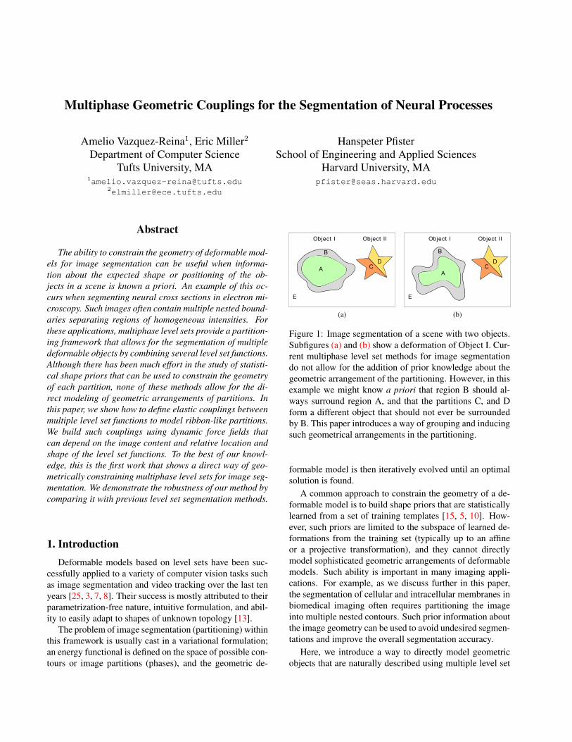
Figure 1: Image segmentation of a scene with two objects.Subfigures (a) and (b) show a deformation of Object I. Cur-rent multiphase level set methods for image segmentationdo not allow for the addition of prior knowledge about thegeometric arrangement of the partitioning. However, in thisexample we might know a priori that region B should al-ways surround region A, and that the partitions C, and Dform a different object that should not ever be surroundedby B. This paper introduces a way of grouping and inducingsuch geometrical arrangements in the partitioning.

formable model is then iteratively evolved until an optimalsolution is found.

A common approach to constrain the geometry of a de-formable model is to build shape priors that are statisticallylearned from a set of training templates [15, 5, 10]. How-ever, such priors are limited to the subspace of learned de-formations from the training set (typically up to an affineor a projective transformation), and they cannot directlymodel sophisticated geometric arrangements of deformablemodels. Such ability is important in many imaging appli-cations. For example, as we discuss further in this paper,the segmentation of cellular and intracellular membranes inbiomedical imaging often requires partitioning the imageinto multiple nested contours. Such prior information aboutthe image geometry can be used to avoid undesired segmen-tations and improve the overall segmentation accuracy.

Here, we introduce a way to directly model geometricobjects that are naturally described using multiple level set

functions. As opposed to most of the previous work onmulti-shape learning for deformable models [20, 12], ourmethod does not rely on the statistical inference of a multi-shape distribution from a set of training samples. We in-stead provide a way to directly design entire families ofpartition arrangements using dynamic force fields that candepend on the image content and multiple level set func-tions. There are a number of important application areaswhere such an approach is useful. Consider the example ofFig. 1 that shows a scene with two objects and the back-ground. A classical multiphase method for segmentationwould partition the scene into several phases according toimage features (gradient, statistical variance, etc.), and op-tionally, according to some statistically learned shape priorfor each of the partitions. Such approaches do not allow forthe addition of prior knowledge about the relative arrange-ment of the regions in the partitioning. A real example ofthis idea can be seen when tracking neural processes (cellu-lar and intra-cellular boundaries) in a sequence of sectionsfrom a 3D volume of brain tissue. In each section, cells,mitochondria and other intra-cellular objects have a mem-brane of homogeneous intensity and varying thickness (seean example in Fig. 2). The tracking of these processes isof important interest in neuroscience, where scientists areaiming at identifying and analyzing the internal wiring ofthe brain.

The main contributions of our work are first, the defi-nition of elastic couplings between level set functions us-ing dynamic force fields that can be easily integrated inany variational-based multiphase framework, and second,the modeling of ribbon-like deformable models that can beused to segment and track neural processes. To the best ofour knowledge none of these issues have been addressed todate.

2. Related workVariational and energy minimization models for image

segmentation based either on level sets or graph cuts arewell documented in the literature [25, 2, 22]. For multi-object segmentation, multiway graph cuts and multiphasegraph cuts and level sets provide a natural extension of thesingle object case [22, 19, 18, 21]. In the multiphase levelsets literature, much attention has gone into the study oftopologically constrained flows that avoid vacuum regionsand overlap between the different phases [3, 17, 26, 24],and into extending shape priors for single level set evolu-tions to the multiphase case [6, 4, 9, 12]. Two interestingproblems have been addressed in this last area, first, iden-tifying which shape prior should be applied to which levelset function (this process is also known as shape prior com-petition) [6, 4], and second, applying shape priors while al-lowing for mergers and splits of multiple phases [9].

Very recently, there has been an effort to employ exter-

Figure 2: Example of a cross section of a 3D volume ofbrain tissue acquired with an electron microscope (1px. =3nm x 3nm). Given the nature of the images, we can safelymake the assumption that sections can be decomposed intoa set of “ribbons” of varying thickness.

nal force fields within the multiphase level set framework ina manner which preserves the underlying, assumed known,topology of the problem [7]. Our work shares some similar-ities with this work. Mostly, we both consider the integra-tion of external force fields in multiphase level sets and theirapplication in segmentation. However, our work focuses onhow to induce a geometrical arrangement on the differentphases, while the work of [7] focuses on preserving thetopology of the different phases and avoiding vacuum re-gions and overlap altogether.

3. Minimum partition with multiphase levelsets

To motivate our work, we consider the classical twodimensional grayscale piecewise-constant segmentationproblem in computer vision known as the minimal partitionproblem or the Mumford and Shah problem. This problemwas originally formulated in [16], and since then, severalvariations have appeared in the literature. In the follow-ing we introduce a variation of the so called reduced model[21] of this problem: Let Ω ∈ R2 be open and bounded,then, given an observed image u, we seek a decomposi-tion G = (Ω1, . . . ,Ωm) of Ω and a vector of constantsc = (c1, . . . , cm) such that the following energy is mini-mized:

E (G, c) =m∑i=1

(λi

∫Ωi

(u− ci)2dx+

αi2

∫Γi

ds

)(1)

(a) (b)

Figure 3: (a): We make the assumption that any cross sec-tion of the brain tissue can be decomposed into a set of “rib-bons”. (b): In the simplified case where we only have oneribbon, the ribbon partitions the image into three differentphases. According to our multiphase encoding of Eq. (2),we need at least two distance field functions φ1 and φ2 torepresent three phases.

where Γi represents the boundary set of each partition Ωiand the tuning parameters λi ≥ 0 and αi ≥ 0 weigh therelative importance of the different terms in the energy. Theabove energy favors intensity smoothness along each parti-tion and penalizes the size of their boundary sets.

In order to translate the above problem into a multiphaseformulation, we use n = log2m level set functions andfollow the implementation in [21], which guarantees novacuum and overlap between phases. In this framework, avector level set function Φ is defined as Φ = (φ1, . . . , φn)where each φi : Ω → R is a level set function. Similarly, apartition Ωi is represented by a binary vector Ki of lengthn. This way, we can define the characteristic function χi foreach partition Ωi as follows:

χi =

1 when (H (φ1) , . . . ,H (φn)) = Ki

0 otherwise(2)

where (H (φ1) , . . . ,H (φn)) is a binary vector that takesdifferent values when evaluated in different partitions of theimage. The function H (φ) takes the values H (φ) = 0when φ ≤ 0 and H (φ) = 1 when φ > 0.

We can now rewrite Eq. (1) in terms of the level setfunctions as:

E (Φ, c) =m∑i=1

(λi

∫Ω

(u− ci)2χidx+

αi2

∫Ω

|∇χi|)(3)

Notice that our level set representation uses the same num-ber of level set functions as [21] and [6], and is differentfrom the work of [3, 9, 19], where one level set functionper partition was used instead, and from [7] where only atotal of four functions were needed. The Euler-Lagrangeequation corresponding to the gradient descent of the func-tional in Eq. (3) yields a system of n evolution equationsfor (φ1, . . . , φn) (see [21] for an example of a four-phasesystem).

Figure 4: Force field for ribbon consistency. The iso-linesof φ1 and φ2 are depicted in blue and red, respectively. De-pending on the sign of σ1 and σ2, the force field wouldattract or repel the boundaries of the ribbon. In the casedisplayed, both σ1 and σ2 are considered to be positive.

4. Adding geometric priors to the multiphaseframework

The variational formulation of Eq. (1) only uses what areconventionally called internal terms (those associated withthe regularity of the interface), and data terms (those asso-ciated with the image data). There is nothing in such for-mulation that constrains the relative shape and positioningof the partitions. In the present section, we present a wayof controlling the geometric arrangement of the partition-ing by coupling several phases using dynamic force fields.These force fields will generate velocities for each partitionthat will be added to those generated by the gradient descentof the Mumford Shah (MS) functional. First, we recall therelationship between curve evolution, level sets and theirconnection with force fields.

The Level Set Method allows to connect the propaga-tion of a 2D front γ to the evolution of the zero level setof a function φ (γ, t). This way, γ propagates with a speedγt ∈ TγM , if and only if, by the chain rule, φ propagatesaccording to the Level Set equation:

∇φ (γ, t) · γt + φt = 0 (4)

where TγM ∈ R2 is the tangent space of the manifoldM of closed curves immersed in R2, defined at γ [14].The n evolution equations for (φ1, . . . , φn) that result fromthe gradient descent of the MS functional in Eq. (3) prop-agate the zero-level sets of each φ function with speeds(γMS

1t , . . . , γMSnt

)due to the connection established by the

Level Set Method. Since the encoding of each partition inEq. (2) links the evolution of each level set function withthe evolution of each partition, the gradient flow also im-plicitly propagates each partition (Ω1, . . . ,Ωm) with speedsthat we denote as

(ΓMS

1t , . . . ,ΓMSmt

). These velocities result

from the optimization of the minimum partition problem,and therefore have a variational nature.Consider now a vector field v : Ω→ R2. We can build a ve-

Figure 5: σ1 as a function of φ2 The graph for σ2 is obtainedby reversing the φ axis (σ2 (φ) = σ1 (−φ)). The regionlabeled as A corresponds to the attraction (σ1 ≥ 0, v1 ≥ 0)between the ribbon boundaries (stronger as the boundariesseparate from each other). Region B is the region wherethe ribbon shows a plastic behavior (no resistance towardsdeformation). Region C corresponds to the repulsion (σ1 ≤0, v1 ≤ 0) between the ribbon boundaries (stronger as theboundaries come closer to each other).

locity field γvit for the zero-level set of one of our functionsφi if we project v on Tγi

M via the mapping γvit = v · γ⊥i .Such mapping extracts the normal component of v to thezero level set of φi. As in the Mumford Shah case, the vec-tor field v implicitly also maps into a vector of velocities(Γv1t, . . . ,Γ

vmt) for each of the boundary sets of the parti-

tions.We can extend this concept to build a force field F =

(v1, . . . , vn) for each zero-level set γi. In the more gen-eral case, we can generate p force fields that, if designedwisely, could be used to arrange the different partitions(Ω1, . . . ,Ωm) on the plane. Since TγM is a vector space,the velocity fields derived from such force fields can beadded to the velocities derived from the MS functional asfollows:

γt = γMSt +

p∑j=1

µjγFj

t (5)

where γt = (γ1t, . . . , γnt) is the vector of total veloci-ties of the zero-level sets, γMS

t =(γMS

1t , . . . , γMSnt

)is

the vector of velocities given by the gradient descent ofthe MS functional, and γ

Fj

t =(γv1j

1t , . . . , γvnj

nt

)is the

vector of velocities given by the action of the force fieldFj = (v1j , . . . , vnj) onto each of the φ functions. The pa-rameters µj determine the strength of the force fields rela-tive to that arising from the MS functional.

It is important to note, however, that since the vec-tor fields v don’t have to be irrotational (curl-free), someof them might not equal the gradient of a scalar poten-tial, and therefore it is not always possible to guaranteethe existence of an equivalent variational formulation foreach vector field. For this reason, we will consider that asolution for the segmentation problem is found (the evo-lution finishes) when the velocities from the optimizationof the MS functional and those from the external force

Figure 6: We want the outer side of the active ribbon(φ2 = 0) to be attracted towards the outer side of the cel-lular membrane (feature map in green), and the inner sideof the ribbon (φ1 = 0) towards the inner cellular membrane(feature map in pink).

fields balance each other and an equilibrium is reached(||(γ1t, . . . , γnt)||L2 ≤ ε). In the best case, the velocitiesfrom the MS functional balance their counterparts from theforce fields Fj :

γMSt = −

p∑j=1

µjγFj

t (6)

In the next section we show several examples of forcefields that can be used to induce geometrical arrangementsin the partitioning.

5. Active Ribbons

Consider again the problem of segmenting and track-ing neural processes presented in the introduction. Neu-ral membranes can be composed of myelin in the case ofaxons, and the analysis of their thickness can reveal impor-tant information about the connectivity of biological neuralnetworks and neural-related diseases [1]. For this reason itwould be useful to be able to segment and extract each ofthe membranes in an isolated partition. This allows us to usethe ideas from the previous section to model such geometricpartitioning.

We start by defining an active ribbon as the deformableregion between two non-intersecting contours, one con-tained within the other. Figure 3(a) shows that a single ac-tive ribbon yields a partitioning of the image in three regions(inside, ribbon and outside). According to our multiphaseencoding of Eq. (2), we need at least two distance fieldfunctions φ1 and φ2 to represent three regions.

We now consider three force fields that can be used toarrange the image partitions into a set of ribbons. The firsttwo forces control the shape of each ribbon and their abilityto find the right cellular boundaries in an image of braintissue. The third one is required for problems where wewish to track simultaneously multiple neurons and modelsthe interaction between ribbons by controlling their mutualrepulsion or attraction.

(a) (b)

Figure 7: (a): Active ribbon (in green) on a sample image.(b): Normalized feature maps e1 (left) and e2 (right) for theinner and outer side of the ribbon (blue).

5.1. Force field for ribbon consistency

Consider the force field:

F1 (v1, v2) =(∇φ2

σ1,−∇φ1

σ2

)(7)

where v1 and v2 act on φ1 and φ2, respectively, and σ1 andσ2 are scalar fields defined on the image plane. The jointaction of v1 and v2 creates a repulsion or an attraction forcebetween the boundaries of the ribbon depending on the signof σ1 and σ2 (see Fig. 4). Ideally, we want to design the rib-bon so that it shows plasticity (no resistance to deformation)when the thickness of the ribbon is within some reasonablerange (5-20 nm.). In such cases, the evolution of the rib-bons would be mostly driven by the gradient flow of theMS functional Eq. (1). On the other hand, we want to trig-ger the repulsion or attraction between the boundaries of theribbon when the ribbon has an abnormal thickness. Follow-ing this reasoning, we can design σ1 and σ2 for φ1 and φ2

so that they react to the proximity between the boundariesof the ribbons. We can achieve this effect by setting σ1 (φ2)and σ2 (φ1) with a profile such as the one depicted in Fig.5. A piecewise polynomial approximation of this profile isdiscussed in Section 6.

5.2. Force field for ribbon-cell interaction

The previous force field model adds a purely geometricforce to the multiphase partitioning by inducing the creationof elastic ribbons. The combination of such force field withthe MS functional will segment the image in homogeneousribbon-like partitions. However, the model so far does notnecessarily guarantee that the two different boundaries ofthe ribbon will be attracted to different boundaries of thecellular membranes (see Fig. 6). In this section we intro-duce a second force field that, when added to the previousmodel, achieves precisely that.

We start by recalling the vector field convolution model

(a) (b)

Figure 8: (a): Close-up of component v1 of Force field F2

generated from the ribbon and sample image in Fig. 7(a).The vector field points towards the inner side of the cellularmembranes (b): User defined vector kernel for vector fieldconvolution. See [11] for more details on different types ofkernels.

introduced in [11]. Given a feature map defined on the im-age e : Ω → R+ (i.e. a bitmap) we can build a smoothvector field v (vx, vy) : Ω → R2 that points towards thehighest values in e as:

(vx, vy) = e ∗ k = (e ∗ kx, e ∗ ky) (8)

where k(kx, ky) is a 2D user-defined vector field kernelsuch as the one shown in Fig. 8b, and the subscripts re-fer to the x and y components of each vector field. See [11]for additional notes on kernel selection.

Building on this idea, consider the following force field:

F2 (v1, v2) = (e1 ∗ k, e2 ∗ k)= ((∇Iσ · ∇φ1) ∗ k,− (∇Iσ · ∇φ2) ∗ k) (9)

where Iσ is a smoothed version of the image I, and e1 =∇Iσ · ∇φ1 and e2 = −∇Iσ · ∇φ2 are the feature maps forφ1 and φ2, respectively. The above force field is made of avector field v1 that acts on φ1 by pushing its zero-level settowards the inner side of the cellular boundaries, and v2 thatacts on φ2 by pushing its zero-level set towards their outerside (see Fig. 6). Figures 7 and 8(a) show the feature mapsand the resulting force field on examples of real images.

5.3. Interaction between ribbons

The previous two force fields control the shape and seg-mentation of each ribbon in an individual manner, andtherefore they do not offer control over the interaction ofneighboring structures. However, going back to our ap-plication of interest (tracking of neural boundaries), it isknown that when moving from one section to the next onethrough the 3D volume of brain tissue, the cellular bound-aries of the neurons should not change their relative positionabruptly. That is, if two neurons were adjacent to each other

(a) (b)

Figure 9: (a): A force of mutual repulsion or attraction iscreated between each pair of ribbons based on the resultfrom previous sections. (b): σI is chosen to create a elasticrepulsion (region A) or attraction force (region C) to keepthe distance between the ribbons within some range (regionB).

and/or relatively close in one section, they should be so inthe next one. We can take advantage of this fact and con-trol the geometric arrangement of the partitioning furtherto avoid undesired segmentations and speed up the conver-gence of the multiphase evolution.

Consider that while processing section i of the volumeof brain tissue we are given the segmentation results fromsection i− 1. Since we know the location of each ribbon insection i, we can build a force field Fab (v1, v2, v3, v4) foreach pair of ribbons a and b, such that:

v = σI (|abi| − |abi−1|) abiv1 = v2 = v, v3 = v4 = −v (10)

where the vectors abi and abi−1 are the vector that pointsfrom the center of mass of a to the one of b, and σI : R→ Ris a function that controls the strength of the mutual repul-sion (σI < 0) or attraction (σI > 0) between the two rib-bons (see Fig. 9). Section 6 discusses a piecewise polyno-mial approximation of σI .

6. ExperimentsIn this section we present several experiments that show

the robustness of our active ribbons model on real data.First, we compare our model with three other well knownlevel set-based deformable models for the segmentation ofsingle cellular boundaries. We then compare our methodwith a geometrically-unconstrained multiphase level setmodel for the segmentation multiple cellular boundaries.Finally, we show how our active ribbon model can effi-ciently track cellular boundaries on a sequence of cross-sections obtained from a volume of brain tissue and givean example of failed segmentation.

Figure 10 shows a comparison of our model with sev-eral geometrically-unconstrained deformable models. Inthe best cases, these models were able to accurately extract

Figure 10: First row: Best result obtained using the mod-els of [11] and [23] with the deformable model initial-ized with a single connected component from outside. Sec-ond and third row: Results obtained using the two-phasemodel of [21] when the deformable model was initializedfrom outside, and from both inside and outside, respec-tively; Similar results were obtained with this initializationfor the models of [11] and [23]. Fourth row: Results ob-tained with the model of [17] with region descriptors basedon the mean and variance for both the foreground and back-ground. Fifth row: Results obtained with our active ribbonmodel. The columns correspond to iterations 1, 34 and 71.

the outer cellular boundaries or the inner cellular bound-aries alone, but none of them could segment the cellularmembranes in a single isolated partition, making them in-valid for the analysis and study of myelin thickness. Theparameters chosen for the ribbon-consistency force field inthe last row were |b| = 10px and |c| = 25px and a = 10−9.

Figure 11 shows a gradual comparison between a classi-cal geometrically-unconstrained multiphase level set modeland our active ribbon model. The parameters chosen forthe ribbon-to-ribbon interaction force were d = 50px ande = 2px. It is important to note that in our model, by us-ing two level set functions to represent each ribbon, we al-low the ribbons to overlap on the image. This overlap isa consequence of our partition encoding of Eq. (2), where

Figure 11: Gradual comparison between a classical geometrically-unconstrained multiphase level set model and our activeribbon model. First row: Results obtained with the model of [21] with λi set to 0 for the background phases in Eq. (3).Second row: Results obtained with our force field for ribbon consistency. Third row: Results obtained with all the force fieldsdiscussed in the paper enabled. The columns correspond to iterations 1, 34, 55 and 79.

the zero-level sets of multiple level set functions can inter-sect. This encoding uses a total of 2m level set functionsfor m ribbons, but gives direct access to each ribbon viatheir zero-level sets. Such encoding also guarantees thatribbons can share cellular boundaries and therefore agreeswith the biological model of neural membranes in cellularbiology. Finally, such overlap facilitates the tracking of neu-rons throughout the volume of brain tissue, since this wayeach ribbon can more easily sit on image boundaries.

Figure 12 shows the tracking of a neural process, wherein each section, the active ribbon model is initialized withthe results obtained in the previous cross-section of thebrain tissue. Such approach to tracking only works a neuralprocess is orthogonal to the image plane, since otherwiseneural processes would experiment large displacements be-tween consecutive sections.

Finally, Fig. 13 shows an example of a failed segmenta-tion with one ribbon, where the presence of multiple adja-cent cellular membranes confused the ribbon to believe it issegmenting a single process.

The active ribbon parameters for the examples of Fig. 10and Fig. 11 were µ1 = 1.5, µ2 = µ3 = 1 and αi = λi = 1for the foreground phases and 0 for the background ones.The parameters for Fig. 12 were: µ1 = 1, µ2 = 0.35, andsame αi’s and λi’s as in the segmentation examples. Thefunction graphs of Figs. 9 (b) and 5 were approximatedusing quadratic polynomials that interpolate the point coor-dinates derived from the horizontal and vertical lines corre-sponding to the parameters a, b, c, d and e. Large variations

Figure 12: Left-to-right and top-to-bottom: Tracking of acellular membrane that is orthogonal to the scanning plane.The active ribbon is initialized with the results obtained inthe previous cross-section of the brain tissue.

of appearance of neural processes were accounted by in-creasing the overall elasticity of the model, which can becontrolled with σ1, σ2 and σI .

Figure 13: Example of a failed segmentation with one rib-bon. The images correspond to iterations 1, 10, 16 and 30.

7. Conclusions and future workThis paper is, to the best of our knowledge, the first work

that shows a direct way of geometrically constraining a mul-tiphase level sets flow for image segmentation. This is doneusing dynamic force fields such as those introduced previ-ously in the literature for active contours for helping themdeal with local minima. Our method requires no trainingset and can be easily combined with other variational levelset segmentation models. Future work includes extensionsto 3D deformable models, and the study of the ability ofdynamic force fields to induce other possible geometric ar-rangements.

8. AcknolewdgementsThis material is based upon work supported in part by

the National Science Foundation under Grant No. PHY-0835713. We would like to acknowledge the generoussupport from Microsoft Research and the members of JeffLichtman’s lab for providing access to the imagery.

References[1] R. Aharoni, A. Herschkovitz, R. Eilam, M. Blumberg-

Hazan, M. Sela, W. Bruck, and R. Arnon. Demyelina-tion arrest and remyelination induced by glatiramer acetatetreatment of experimental autoimmune encephalomyelitis.PNAS, 105(32):11358–11363, 2008. 4

[2] Y. Boykov and G. Funka-Lea. Graph cuts and efficient n-dimage segmentation. IJCV, 70(2):109–131, Nov. 2006. 2

[3] T. Brox and J. Weickert. Level set segmentation with multi-ple regions. TIP, 15(10):3213–3218, 2006. 1, 2, 3

[4] T. Chan and W. Zhu. Level set based shape prior segmenta-tion. In CVPR, San Diego, CA, USA, June 2005. 2

[5] D. Cremers, S. J. Osher, and S. Soatto. Kernel density es-timation and intrinsic alignment for shape priors in level setsegmentation. IJCV, 69(3):335–351, 2006. 1

[6] D. Cremers, N. Sochen, and C. Schnorr. A multiphase dy-namic labeling model for variational recognition-driven im-age segmentation. IJCV, 66(1):67–81, 2006. 2, 3

[7] X. Fan, P.-L. Bazin, and J. Prince. A multi-compartmentsegmentation framework with homeomorphic level sets. InCVPR, Anchorage, AL, USA, June 2008. 1, 2, 3

[8] K. Fundana, N. C. Overgaard, and A. Heyden. Variationalsegmentation of image sequences using region-based activecontours and deformable shape priors. IJCV, 80(3):289–299,2008. 1

[9] M. Fussenegger, R. Deriche, and A. Pinz. A multiphase levelset based segmentation framework with pose invariant shapepriors. In ACCV (2), pages 395–404, 2006. 2, 3

[10] J. Kim, M. Cetin, and A. S. Willsky. Nonparametric shapepriors for active contour-based image segmentation. SignalProcess., 87(12):3021–3044, 2007. 1

[11] B. Li and S. T. Acton. Active contour external force us-ing vector field convolution for image segmentation. TIP,16(8):2096–2106, 2007. 5, 6

[12] A. Litvin and W. C. Karl. Coupled shape distribution-basedsegmentation of multiple objects. In IPMI, pages 345–356,2005. 2

[13] R. Malladi, J. A. Sethian, and B. C. Vemuri. Shape mod-eling with front propagation: a level set approach. TAPI,17(2):158–175, 1995. 1

[14] P. W. Michor and D. Mumford. Riemannian geometries onspaces of plane curves. JEMS, 8:1–48, 2003. 3

[15] M.Rousson and N.Paragios. Prior knowledge, level set rep-resentations & visual grouping. IJCV, 76(3):231–243, 2008.1

[16] D. Mumford and J. Shah. Optimal approximations by piece-wise smooth functions and associated variational problems.Comm. Pure and App Math., 42(5):577–685, 1989. 2

[17] N. Paragios and R. Deriche. Coupled geodesic active regionsfor image segmentation: A level set approach. In ECCV,pages 224–240, 2000. 2, 6

[18] N. Paragios and R. Deriche. Geodesic active regions andlevel set methods for supervised texture segmentation. IJCV,46(3):223–247, 2002. 2

[19] C. Samson, L. Blanc-Feraud, G. Aubert, and J. Zerubia.Level set model for image classification. IJCV, 40(3):187–197, 2000. 2, 3

[20] A. Tsai, W. Wells, C. Tempany, E. Grimson, and A. Will-sky. Mutual information in coupled multi-shape model formedical image segmentation. MIA, 8(4):429–445, 2004. 2

[21] L. A. Vese and T. F. Chan. A multiphase level set frameworkfor image segmentation using the mumford and shah model.IJCV, 50(3):271–293, 2002. 2, 3, 6, 7

[22] N. Vu and B. Manjunath. Shape prior segmentation of mul-tiple objects with graph cuts. In CVPR, June 2008. 2

[23] C. Xu and J. L. Prince. Generalized gradient vector flowexternal forces for active contours. Sig. Proc., 71:131–139,1998. 6

[24] A. Yezzi, A. Tsai, and A. Willsky. A fully global approach toimage segmentation via coupled curve evolution equations.J. Vis. Comm. Img. Rep., 13(1-2):195–216, 2002. 2

[25] J. Yezzi, A., A. Tsai, and A. Willsky. A statistical approachto snakes for bimodal and trimodal imagery. In ICCV, 1999.1, 2

[26] H.-K. Zhao, T. Chan, B. Merriman, and S. Osher. A varia-tional level set approach to multiphase motion. J. Comput.Phys., 127(1):179–195, 1996. 2