Multiphase Flow Modeling for Design and Optimization of a ...
232
Louisiana State University LSU Digital Commons LSU Doctoral Dissertations Graduate School 12-13-2017 Multiphase Flow Modeling for Design and Optimization of a Novel Down-flow Bubble Column Mutharasu Lalitha Chockalingam Louisiana State University and Agricultural and Mechanical College, [email protected] Follow this and additional works at: hps://digitalcommons.lsu.edu/gradschool_dissertations Part of the Aerodynamics and Fluid Mechanics Commons , Computational Engineering Commons , Computer-Aided Engineering and Design Commons , and the Transport Phenomena Commons is Dissertation is brought to you for free and open access by the Graduate School at LSU Digital Commons. It has been accepted for inclusion in LSU Doctoral Dissertations by an authorized graduate school editor of LSU Digital Commons. For more information, please contact[email protected]. Recommended Citation Lalitha Chockalingam, Mutharasu, "Multiphase Flow Modeling for Design and Optimization of a Novel Down-flow Bubble Column" (2017). LSU Doctoral Dissertations. 4181. hps://digitalcommons.lsu.edu/gradschool_dissertations/4181
Transcript of Multiphase Flow Modeling for Design and Optimization of a ...

Louisiana State UniversityLSU Digital Commons
LSU Doctoral Dissertations Graduate School
12-13-2017
Multiphase Flow Modeling for Design andOptimization of a Novel Down-flow BubbleColumnMutharasu Lalitha ChockalingamLouisiana State University and Agricultural and Mechanical College, [email protected]
Follow this and additional works at: https://digitalcommons.lsu.edu/gradschool_dissertations
Part of the Aerodynamics and Fluid Mechanics Commons, Computational EngineeringCommons, Computer-Aided Engineering and Design Commons, and the Transport PhenomenaCommons
This Dissertation is brought to you for free and open access by the Graduate School at LSU Digital Commons. It has been accepted for inclusion inLSU Doctoral Dissertations by an authorized graduate school editor of LSU Digital Commons. For more information, please [email protected].
Recommended CitationLalitha Chockalingam, Mutharasu, "Multiphase Flow Modeling for Design and Optimization of a Novel Down-flow Bubble Column"(2017). LSU Doctoral Dissertations. 4181.https://digitalcommons.lsu.edu/gradschool_dissertations/4181

i
MULTIPHASE FLOW MODELING FOR DESIGN AND OPTIMIZATION
OF A NOVEL DOWN-FLOW BUBBLE COLUMN
A Dissertation
Submitted to the Graduate Faculty of the
Louisiana State University and
Agricultural and Mechanical College
in partial fulfillment of the
requirements for the degree of
Doctor of Philosophy
in
The Gordon A. and Mary Cain Department of Chemical Engineering
by
Mutharasu Lalitha Chockalingam
B.Tech., Anna University, 2012
May 2018

ii
Acknowledgements
First, I would like to thank my advisor, Professor Krishnaswamy Nandakumar for his
tireless guidance and support throughout my doctorate program and for going way beyond his
professional responsibilities to be a personal life mentor.
I would like to thank Professor J. B. Joshi for co-advising my project and for providing his time
and wealth of experience in the field of Bubble column flow research.
I would like to thank Dr. Mayur Sathe for his enormous effort spent in training and mentoring me
during the initial phase of my research work, and also for his continued support throughout my
doctorate program.
I would like to thank Dr. Dinesh V Kalaga and his colleagues at City College of New York, for
their tireless efforts in carrying out the experiments on the novel down flow bubble column.
I would like to thank Professor Geoffry Evans for kindly providing me with the experimental data
for the plunging jet bubble column flows.
I would like to pay courtesy to past and present members of the EPIC research consortium, Dr.
Rupesh K Reddy Guntaka, Dr. Yuehao Li , Dr. Abhijit Deshpande, Dr. Gongqiang He, Dr.
Chenguang Zhang, and fellow graduate students, Aaron, Jielin, Daniel, John, Sharareh and Sai.
Finally, I would like to dedicate this dissertation to my father the late Mr. Chockalingam Muthia,
my mother Mrs. Lalitha Dakshinamoorthy, and my sister Uma Lalitha Chockalingam. I would not
have made it this far without their support and unconditional love.
iii
Table of Contents
Literature review on past studies on down-flow bubble columns ................................................. 2 Novel micro-bubble generation mechanism .................................................................................. 5 Need for computational fluid dynamics (CFD) models ................................................................ 6
Euler-Euler model ....................................................................................................................... 13 Turbulence modelling ................................................................................................................. 15 Interfacial force modelling .......................................................................................................... 16
Introduction ................................................................................................................................. 24 Experimental data ........................................................................................................................ 27 CFD setup .................................................................................................................................... 28 Sigmoid function based drag modification for capturing the gas entrainment by the plunging
liquid jet....................................................................................................................................... 31 CFD results .................................................................................................................................. 40 Linear stability analysis ............................................................................................................... 45 Conclusions ................................................................................................................................. 54
Introduction ................................................................................................................................. 55 Experimental setup and data........................................................................................................ 55 Population balance model (PBM) ............................................................................................... 58 PBM kernels: ............................................................................................................................... 60 Modelling of the array of liquid jets in a periodic domain .......................................................... 65 Full reactor scale modelling, CFD-PBM setup ........................................................................... 70 Results ......................................................................................................................................... 75 Mass transfer modelling .............................................................................................................. 79 RTD studies from CFD-PBM model........................................................................................... 82
Conclusions ................................................................................................................................. 86
Introduction ................................................................................................................................. 87 Experimental setup: ..................................................................................................................... 88 Drag modification factor from force balance method ................................................................. 94 CFD simulation setup .................................................................................................................. 99 Results and discussion ............................................................................................................... 103 Conclusions ............................................................................................................................... 122
Introduction ............................................................................................................................... 124
Acknowledgements ....................................................................................................................................... ii
Abstract …. .................................................................................................................................................. v
Chapter 1. General Introduction .................................................................................................................. 1
Chapter 2. Euler-Euler Modelling Framework for Bubbly Flows (Gas-Liquid) ...................................... 13
Chapter 3. Modelling of a Plunging Jet Bubble Column with Variable Free Jet Length ......................... 24
Chapter 4. CFD-PBM Modelling of a Novel Down Flow Bubble Column .............................................. 55
Chapter 5. CFD Study of the Extent and Nature of Liquid Circulations in a Novel Down-Flow Bubble
Column of 30 cm Column Diameter ....................................................................................... 87
Chapter 6. Design Optimizations for the Novel Down Flow Bubble Column Based on CFD ............... 124

iv
Perforated plate design .............................................................................................................. 124 Gas sparger design .................................................................................................................... 135 Conclusions ............................................................................................................................... 142
Introduction ............................................................................................................................... 143 Drift flux model ......................................................................................................................... 143 1D performance model .............................................................................................................. 150 Conclusions ............................................................................................................................... 165
Chapter 7. One Dimensional Performance Model .................................................................................. 143
Chapter 8. Summary ............................................................................................................................... 166
References . ............................................................................................................................................... 170
Appendix A: C-Code for Sigmoid Drag Modification, Used in Section 3.4 ............................................ 177
Appendix B: C-Code for Source-Point Modelling and RTD Simulations, Used in Chapter 4. ................ 179
Appendix C: MATLAB Optimization Routine for Drag Modification Function Used in Section 5.3 ..... 196
Appendix D: C-Code for Source-Sink Modelling of the Jet Region, Used in Section 5.4 ....................... 205
Appendix E: MATLAB Script for solving the 1D performance model, Used in Section 7.3 .................. 218
Vita ..……. ............................................................................................................................................... 226
v
Abstract
The application of the Euler-Euler framework based Computational Fluid Dynamics (CFD)
models for simulating the two-phase gas-liquid bubbly flow in down-flow bubble columns is
discussed in detail. Emphasis is given towards the modelling and design optimization of a novel
down-flow bubble column. The design features of this novel down-flow bubble column and its
advantages over a conventional Plunging Jet down-flow bubble column are discussed briefly.
Then, some of the present challenges in simulating a conventional Plunging Jet down-flow bubble
column in the Euler-Euler framework is highlighted, and a sigmoid function based drag
modification function is implemented to overcome those challenges. The validated CFD results
are further utilized for performing a linear stability analysis.
We then discuss the applicability of a coupled CFD-PBM (Population Balance Model) to
simulate the micro-bubble generation process in the novel down-flow bubble column of small
cross-section of 10 cm diameter. For a much larger column of 30 cm diameter, due to high
computational requirements and lack of accurate breakage kernels in the PBM, we model the
micro-bubble generation process using the Euler-Euler model with appropriate source and sink
terms to represent the region where micro-bubbles are generated. Further, a force-balance based
method is used to determine the appropriate drag correlation and the associated local gas hold-up
based drag modification functions. The developed CFD modelling approach, is then used to
perform design explorations and optimization to improve the performance of the novel down-flow
bubble column design. Finally, a one dimensional performance model is derived for the down-
flow bubble column. This simple model could be used for scale-up analysis, to provide rough
estimates of the performance of a down-flow column of arbitrary length.

1
Chapter 1. General Introduction
Bubble column reactors are widely used as gas-liquid contactors due to their simple
construction, lack of mechanical parts and efficient mixing and mass transfer characteristics.
Bubble columns find application in processes such as oxidation, hydrogenation, fermenters and
other bio-reactors etc. (Joshi, 2001). In bubble columns the gas phase is the dispersed phase
consisting of bubbles, and the continuous phase is the liquid phase. The bubbly flow takes place
in two regimes: at low gas injection rates the bubbles are of uniform size and the radial profile of
the gas hold-up is flat and this is characterized as homogeneous regime, and at high gas injection
rates the radial profile of the gas hold-up is no longer flat and this in turn leads to intense liquid
recirculation and this is characterized as heterogonous regime.
Figure 1-1: Illustration of flow circulations in Up-flow and Down-flow bubbly flow conditions.

2
As pointed out in conventional bubble columns due to high gas injection rates, the rise velocity of
the bubbles is comparable to that of the slip velocity of the bubbles. The high rise velocity of the
bubbles leads to decrease in the bubble residence time, which in turn leads to a low gas hold-up of
about 30% (Bhusare et al., 2017; Hills, 1974; Kalaga et al., 2017; Krishna et al., 1999; Menzel et
al., 1990; Yu and Kim, 1991). Down-flow bubble columns are of interest, as the gas is forced to
move downward against its natural tendency to rise, this increases the residence time of the bubbles
and so it is possible to achieve much higher gas hold-ups for a given gas injection rate. This
increase in residence time of the bubbles and the gas hold-up, also leads to increase in interfacial
area concentration and increased mass transfer rates (Majumder et al., 2006a).
Literature review on past studies on down-flow bubble columns
Despite the large literature addressing the experimental and modelling aspects of Bubble
column flows, most of these studies have focused on semi-batch mode and co-current upward-
flow operating conditions. There have been few experimental studies on co-current down-flow
bubble columns and even less focus on the CFD modelling of the same. Table 1-1 summarizes the
previous investigations on down-flow bubble columns, their column diameters and measurement
techniques.

3
Table 1-1: Past studies on down-flow bubble columns
Author
Column
Diameter,
(m)
Measured
parameter
Measurement
Technique Modelling
Shah et al. (1983) 0.075 1 a -
Ohkawa et al. (1984) 0.05-0.07 1 a -
Kulkarni & Shah (1984) 0.075 1,3 b
Bando et al. (1988) 0.07-
0.164
5 d -
Munter et al. (1990) 0.015 1,3 b Stagewise
backmixing model
Yamagiwa et al. (1990) 0.034-
0.07
1 b -
Lu et al. (1994) 0.076 1,2 a,c -
Kundu et al. (1995) 0.0516 1 a -
Evans et al. (2001) 0.051 1,3 a, e -
Mandal et al.( 2005) 0.0516 1,2 a,c -
Majumder et al. (2005) 0.06 6
-
Majumder et al. (2006a) 0.05 1 a -
Majumder et al. (2006b) 0.05 1,2 a,c -
Upadhyay et al. (2009) 0.051 4,6 f Euler-Euler CFD
Corona-Arroyo et al. (2015) 0.013 1,2 a,c -
1-Volumetric hold-up, 2 – bubble size, 3 – mass transfer, 4 – Radial hold-up profiles, 5 – Point
hold-up, 6 – RTD. a – Phase isolation technique for hold-up, b – Pressure Difference Method for
hold-up, c – Photographic bubble size measurement, d – Conductivity probe for hold-up,e –
Point concentration by volumetric titration, f – Gama Ray Densitometry,g – Tracer experiments
for RTD.

4
The difference in the design aspect of these down-flow bubble columns depend on the gas-
liquid injection mechanism employed to create the two-phase bubbly flow dispersion. Shah et al.
(Shah et al., 1983), Kulkarni & Shah (Kulkarni and Shah, 1984) and Munter et al. (Munter et al.,
1990) used a sparger to introduce the gas directly below the liquid inlet. Few other investigators
(Evans et al., 2001a; Ohkawa et al., 1984; Yamagiwa et al., 1990) have used a single plunging
liquid jet to entrain the gas. In recent years, most researchers have used a gas-liquid ejector
assembly to entrain the gas in the liquid. This mechanism is very similar to the plunging liquid jet,
except that the injection nozzle is designed in such a way to create a partial vacuum that enhances
the suction of the gas phase. The sucked gas is then entrained by the plunging action of the liquid
jet (Bando et al., 1988; Kundu et al., 1995; Lu et al., 1994; Majumder et al., 2006a, 2006b, 2005;
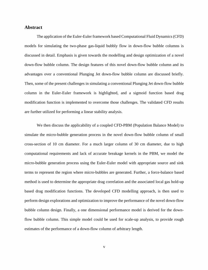
Mandal et al., 2005; Upadhyay et al., 2009). The bubble generation mechanism employed in both
the simple plunging jet and the ejector induced jet columns, involves the entrainment of a sheet of
gas by a single plunging liquid jet, and the subsequent breakage of this sheet of gas due to
instabilities, leading to formation of gas bubbles (Roy et al., 2013). In 0 we discuss in detail some
of the challenges involved in the CFD simulation of a plunging jet down-flow bubble column and
the approach used to overcome those challenges.
5
Figure 1-2: (a) Illustration of a plunging liquid jet entraining the gas from the bulk phase to
dispersed bubbles in the liquid from (Roy et al., 2013); (b) Visualization of the entrainment
action of a plunging liquid jet from (Roy et al., 2013)
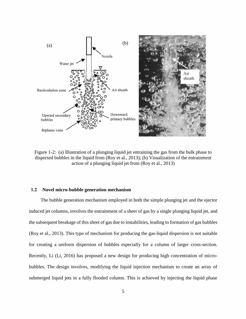
Novel micro-bubble generation mechanism
The bubble generation mechanism employed in both the simple plunging jet and the ejector
induced jet columns, involves the entrainment of a sheet of gas by a single plunging liquid jet, and
the subsequent breakage of this sheet of gas due to instabilities, leading to formation of gas bubbles
(Roy et al., 2013). This type of mechanism for producing the gas-liquid dispersion is not suitable
for creating a uniform dispersion of bubbles especially for a column of larger cross-section.
Recently, Li (Li, 2016) has proposed a new design for producing high concentration of micro-
bubbles. The design involves, modifying the liquid injection mechanism to create an array of
submerged liquid jets in a fully flooded column. This is achieved by injecting the liquid phase
(a) (b)

6
through an orifice plate consisting of a regular arrangement of fine holes, and the liquid emerging
from these holes leads to the formation of the liquid jets. From Chapter 4, onwards the entirety of
this dissertation focuses on understanding the multiphase flow behavior encountered in down-flow
bubble columns that use this novel mechanism of micro-bubble generation.
Figure 1-3: Illustration of the Novel micro-bubble generation mechanism proposed by (Li, 2016)
Need for computational fluid dynamics (CFD) models
In the past, the modelling of the turbulent two-phase gas-liquid flow encountered in bubble
column flows, were modelled using empirical correlations, one-dimensional convection-
dispersion models, or stage-wise segregated models. Most of these models try to establish a

7
relationship between the observed flow pattern and the design parameters like column diameter,
gas and liquid superficial velocities, pressure-drop, gas hold-up, liquid-phase axial mixing, and
mass transfer coefficients at the gas-liquid interface. Most of these models are not reliable for
scale-up and do not necessarily aid in design and performance improvements, as they fail to take
into account the finer details of the flow like the extent of turbulence, liquid-phase circulations and
local variation of the gas hold-up. Recently, in the past two decades owing to the development of
more accurate numerical models especially finite volume Method (FVM) based fluid flow models
for multiphase flows, coupled along with the exponential growth in computational capabilities and
decrease in computational cost, has paved way for CFD to serve as a valuable tool for modelling
the multiphase flow encountered in bubble column flows. Three dimensional CFD models provide
the finer details of the complex multiphase flow in the form of a field data of the three components
of the interstitial velocity of each phase, local gas hold-up and turbulence parameters like turbulent
kinetic energy (k), turbulent dissipation rate (ε) and Reynolds stresses, etc. Figure 1-4 shows the
range and hierarchy of CFD models available based on typical time and length scales of their
applicability.

8
Figure 1-4: Illustration of the hierarchy of CFD models in terms of length and time scales.
For modelling multiphase flows of gas-liquid systems starting from the Kolmogorov length
scale of few micro-meters we have, Direct Numerical Simulation (DNS) models like the high
resolution front tracking method (Tryggvason et al., 2001). The front tracking method involves the
tacking of marker particles in a Lagrangian framework on a fixed background Eulerian grid. It is
computationally very expensive and is not practical for modelling phenomena occurring at reactor
scale. The next set of models involve the Level-set method and Volume of Fluids (VOF) method.
In the Level set methods (Osher and Sethian, 1988) the interface is tracked by the value of an
analytical function that is used to represent the surface of the interface. The VOF method (Hirt and
Nichols, 1981) involves keeping track of the fraction of the computational cell in the Eulerian grid
that is occupied by the fluid of interest. The field data of this fraction of fluid is then used for the
Piecewise linear reconstruction of the interface between the two fluids. VOF method has proved

9
to be very successful in simulating interface phenomena involving surface waves, interface
sloshing and also for problems involving mixing of two or more bulk fluids. The next level of
modelling involves Euler-Lagrangian methods (Lapin and Lübbert, 1994; Webb et al., 1992) were
each bubble or drop in a dispersion is tracked individually in a Lagrangian framework on a Eulerian
background mesh that is used to define the continuous phase. As the number of bubbles
encountered in the simulation domain increases the Euler-Lagrange method gets more and more
computationally expensive in terms of the overload in the memory require to keep track of the
discrete bubbles and also the associated increase in the processing requirements. Finally we have
the Euler-Euler model (Sokolichin and Eigenberger, 1994; Torvik and Svendsen, 1990) where the
gas-liquid dispersion is treated as an interpenetrating continuum. The field values of the fraction
of the dispersed phase (gas) is used to keep track of the concentration of bubbles in a given
computational cell. Figure 1-5 briefly illustrates the difference between each one of these
multiphase flow models that are applicable for gas-liquid flows.

10
Figure 1-5: Illustration of multiphase CFD models for gas-liquid flows: (a) Front tracking
method, (b) VOF method with Piecewise Linear Interface re-Construction (PLIC), (c) Euler-
Lagrangian method, (d) Euler-Euler method.
In chapter 2, we discuss the Euler-Euler model and the k-є turbulence model briefly.We
also describe in detail the interfacial force models like the Drag force, Lift force etc… and the
correlations for the same that are presently available in the literature.
In chapter 3, we present the modelling of a down-flow plunging jet bubble column. The
Euler-Euler model along with a custom drag modification function is employed to simulate the gas
entrainment action of the plunging liquid jet. Further, the three dimensional flow field and
turbulence data obtained from the successful CFD simulations is utilized to perform a linear
stability analysis.

11
In chapter 4, we employ a coupled CFD-PBM model to simulate a novel down-flow bubble
column of 10 cm diameter. This bubble column utilizes the novel micro-bubble generation
mechanism discussed in section 1.2 we discuss the Population Balance Model (PBM) in detail.
And discuss some of the CFD results that provide better insight into the flow behavior encountered
in this novel down-flow bubble column.
In chapter 5, we study the nature of the liquid circulations encountered in a novel down-
flow bubble column of much larger cross-section of 30 cm diameter. We briefly discuss the
different experimental methods that were employed to obtain the bubble-size distribution and local
gas hold-up. The basic Euler-Euler model with appropriate source and sink term modelling is
employed for the CFD simulations. By analyzing both the experimental and CFD results, we arrive
at a better understanding of the nature and extent of liquid circulations encountered in this novel
down-flow bubble column of large cross-section.
In chapter 6, we further demonstrate the application of CFD in carrying out design
explorations and optimizations geared towards improving the performance of these novel down-
flow bubble columns. We focus our attention particularly on optimizing the orifice-plate design
and the gas sparger configuration.
In chapter 7, we review the existing one dimensional flow models like Drift-flux modeling
and finally we derive a one dimensional performance model that incorporates the effect of liquid
axial-dispersion, presence of multiple chemical components in the gas-phase, the inter-face mass
transfer from the gas to liquid phase and also the decrease in the size of the bubbles due to pressure
and mass transfer. This one dimensional performance model will serve as a simple model for scale-

12
up analysis, as it could be utilized for pre-determining the performance of a down-flow bubble
column of arbitrary length.
Finally, in chapter 8 we present a summary of the major contributions of this dissertation.
13
Chapter 2. Euler-Euler Modelling Framework for Bubbly Flows (Gas-
Liquid)
The numerical modelling of gas-liquid systems with a dispersed phase like bubbles, particles
or droplets; have been mostly performed either in the finite volume based Euler-Lagrange (Lapin
and Lübbert, 1994; Webb et al., 1992) or Euler-Euler framework (Sokolichin and Eigenberger,
1994; Torvik and Svendsen, 1990). In the Euler-Lagrange framework, the liquid phase is treated
as continuous and the dispersed gas phase is modelled by tracking individual bubbles in the
Lagrange framework. In the Euler-Euler framework, both the continuous phase (liquid) and
dispersed phase (gas) are treated as interpenetrating continuum. The Euler-Lagrange framework
becomes more computationally expensive as the size of the equipment/computational-domain
increases, because of this the Euler-Euler framework proves to be more economical and is more
widely used. Additional details on the applicability of the Euler-Euler model over the other models
can be found elsewhere (Joshi, 2001).
Euler-Euler model
In reality in the two-phase dispersed bubbly flow encountered in the bubble columns, the actual
flow depends on the
1) Individual bubble deformation and shape oscillations,
2) Bubble-bubble interactions like collision, breakage and coalescence; and
3) Bubble-liquid interactions like drag, lift and associated swarm effects arising due to the
presence of the neighboring bubbles.
The complete understanding of these interactions is still incomplete and also the description of
these interactions within the modelling framework is computationally not practical. For these

14
reasons the following assumptions are made in the derivation of the continuity (Eq.(2-1)) and
momentum (Eq.(2-2)) equations.
1) The gas phase consisting of dispersed bubbles is, treated as a continuum. This makes the
description of entire computational domain as an inter-penetrating continuum.
2) The gas phase is considered to be made of spherical bubbles with a constant diameter.
3) The effect of hydrostatic head on the bubble size, is assumed to be negligible.
4) All interactions between the dispersed phase (gas) and the continuous phase (liquid), is
modelled by the introduction of the interfacial-force terms (section 2.3) in the momentum
equation.
Conventionally for gas-liquid flows encountered in bubble columns, a two-phase Euler-Euler
model is used and it can also be extended to ‘n’ phases leading to a multi-fluid Euler-Euler model.
The following equations are solved for each phase ‘i’ in the multi-fluid Euler-Euler framework.
The injected gas bubbles and the micro-bubbles created in the jet region are treated as two different
phases, so including the liquid phase, three momentum equations (Eq.(2-2)) and two continuity
equations (Eq.(2-2)) are solved. The continuity equation ensures mass balance and the equation of
motion ensures momentum balance in the phase ‘i’. Also, it is to be noted that the flow quantities
being solved for by the field equations ((2-5)) and ((2-6)), are in the time averaged sense and are
not instantaneous values.
𝜕
𝜕𝑡(𝜖𝑖𝜌𝑖) + 𝛻. (𝜖𝑖𝜌𝑖𝑣𝑖) = 0 (2-1)

15
𝜕
𝜕𝑡(𝜖𝑖𝜌𝑖𝑣𝑖) + 𝛻. (𝜖𝑖𝜌𝑖𝑣𝑖𝑣𝑖) = −𝜖𝑖𝛻𝑝 + 𝛻. τi + 𝜖𝑖𝜌𝑖𝑔
+(𝐹𝑑𝑟𝑎𝑔,𝑖 + 𝐹𝑙𝑖𝑓𝑡,𝑖 + 𝐹𝑤𝑙,𝑖 + 𝐹𝑣𝑚,𝑖 + 𝐹𝑡𝑑,𝑖)
(2-2)
Where,
𝜏𝑖 = −𝜇𝑒𝑓𝑓,𝑖(𝛻𝑣𝑖 + (𝛻𝑣𝑖)
𝑇 −2
3𝐼 (𝛻𝑣𝑖) (2-3)
𝜇𝑒𝑓𝑓,𝑖 = 𝜇𝑖 + 𝜇𝑡,𝑖 (2-4)
The pressure velocity coupling is handled by the SIMPLE algorithm (Patankar and Spalding,
1972).
Turbulence modelling
A brief review of the turbulence modelling in two-phase flows, especially in relevance to
taking the field equations from instantaneous quantities to time averaged quantities, and the
subsequent modelling of the statistical correlations involving the fluctuating terms is presented in
(Joshi, 2001). Although, the two equation models like the 𝑘-𝜀 model suffer from the assumption
of isotropic eddy viscosity, they still score over the high fidelity models like the Reynolds stress
model, as they are simple and less computationally demanding. For gas-liquid systems, the mixture
𝑘-𝜀 model (Behzadi et al., 2004) proves to be more reliable for a wide range of dispersed phase
fraction, when compared to earlier works that considered only the turbulent kinetic energy in the
continuous phase. The scalar transport equation solved for the turbulent kinetic energy k and
energy dissipation rate 𝜀 in the mixture 𝑘-𝜀 model are:

16
𝜕
𝜕𝑡(𝜌𝑚𝑘) + 𝛻. (𝜌𝑚𝑘𝑣𝑚) = 𝛻. (
𝜇𝑡,𝑚𝜎𝑘
𝛻𝑘) + 𝐺𝑘𝑚 − 𝜌𝑚𝜀
(2-5)
𝜕
𝜕𝑡(𝜌𝑚𝜀) + 𝛻. (𝜌𝑚𝜀𝑣𝑚) = 𝛻. (
𝜇𝑡,𝑚𝜎𝜀
𝛻𝜀) +𝜀
𝑘(𝐶𝜀1𝐺𝑘𝑚 − 𝐶𝜀2𝜌𝑚𝜀) (2-6)
Where,
𝜌𝑚 = ∑𝜖𝑖𝜌𝑖
𝑁
𝑖=1
(2-7)
𝑣𝑚 =
∑ 𝜖𝑖𝜌𝑖𝑣𝑖𝑁𝑘=1
∑ 𝜖𝑖𝜌𝑖𝑁𝑖=1
(2-8)
𝜇𝑡,𝑚 = 𝜌𝑚𝐶𝜇 ∗
𝑘2
ԑ (2-9)
𝐺𝑘,𝑚 = 𝜇𝑡,𝑚(𝛻𝑣𝑚 + (𝑣𝑚)𝑇): 𝛻𝑣𝑚 (2-10)
Where the mixture k-𝜀 model constants have the same value as in the single-phase k-𝜀 model:
𝐶µ = 0.09, 𝜎𝑘 = 1.00, 𝜎𝜀 = 1.00, 𝐶𝜀1 = 1.44 and 𝐶𝜀2 = 1.92.
Interfacial force modelling
The terms 𝐹𝑑𝑟𝑎𝑔,𝑖 , 𝐹𝑙𝑖𝑓𝑡,𝑖, 𝐹𝑤𝑙,𝑖, 𝐹𝑣𝑚,𝑖, 𝐹𝑡𝑑,𝑖 in the momentum equation (Eq.(2-2)) represent
the interfacial forces between the dispersed phase (gas) and the continuous phase (liquid). These
forces arise due to the relative motion of the bubbles and the liquid, and act on the gas-liquid
interface.

17
2.3.1 Drag force
Among all the interphase forces, the drag force plays a dominating role in predicting the
hydrodynamics of bubbly-flows. When the relative velocity (slip velocity) is constant, then force
acting along the direction of motion is called the drag force (𝐹𝑑𝑟𝑎𝑔).
𝐹𝑑𝑟𝑎𝑔 =
𝐴𝑖8𝐶𝐷𝜌𝐿 |(𝑣𝐺 − 𝑣𝐿)|(𝑣𝐺 − 𝑣𝐿), 𝑤ℎ𝑒𝑟𝑒 𝐴𝑖 =
6𝜖𝐺(1 − 𝜖𝐺)
𝑑𝐵 (2-11)
Where, 𝐶𝐷 is the drag coefficient estimated from a drag closure correlation. Magnaudet & Eames
(2000), have highlighted the importance of developing more accurate closures for evaluating the
interphase forces, and have also pointed out that the current models fail to capture the effect of
processes like bubble deformation, wake instability, surfactant/ Marangoni effect etc. on the
interphase forces. Although once considered as an intractable problem, these models are now being
actively taken on by researchers working on DNS of fully resolved bubbly flow simulations. Most
of these works involve the use of either the Front Tracking method (Ma et al., 2015) or the Lattice
Boltzmann method (Sankaranarayanan et al., 2002; Sankaranarayanan and Sundaresan, 2002).
Although the results from the fully resolved bubbly flow simulations seem to be promising, the
incorporation of these closures in the coarse grid models (Euler-Euler or Euler-Lagrange) is yet to
be adequately tested and validated. Nevertheless, for the time being the empirical models that have
been conventionally used in the Two-Fluid-Model formulation can be utilized with some
modifications. Table 2-1 lists some of these commonly used drag models and their formulations
(Clift et al., 1978; Dalla Ville, 1948; Frank et al., 2005; Laı́n et al., 2002; Ma and Ahmadi, 1990;
Mei et al., 1994; Schiller and Naumann, 1935; Tomiyama, 2004; Tomiyama et al., 1998; Zhang
and Vanderheyden, 2002). Most of the Drag correlations are functions of bubble Reynolds number

18
(ReB) and often give different estimates of the drag force even for the same range of ReB (Pang
and Wei, 2011).
Table 2-1: List of drag correlations
Investigators Drag Coefficient Expression
Schiller and
Naumann (1935) 𝐶𝐷 = {
24(1 + 0.15𝑅𝑒𝐵0.687)
𝑅𝑒𝐵 , 𝑅𝑒𝐵 < 1000
0.44 , 𝑅𝑒𝐵 ≥ 1000
Dalla Ville (1948) 𝐶𝐷 = (0.63 +4.8
√𝑅𝑒𝐵)
2
Clift et al. (2005) 𝐶𝐷 =
{
29.1667
𝑅𝑒𝐵−3.8889
𝑅𝑒𝐵2 + 1.222 , 1 < 𝑅𝑒𝐵 < 10
(24
𝑅𝑒𝐵) (1 + 0.15𝑅𝑒𝐵
0.687) , 10 < 𝑅𝑒𝐵 ≤ 200
Ma and Ahmadi
(1990) 𝐶𝐷 =
24
𝑅𝑒𝐵 (1 + 0.1𝑅𝑒𝐵
0.75)
Mei et al. (1994) 𝐶𝐷 = 16
𝑅𝑒𝐵{1 + [
8
𝑅𝑒𝐵+1
2(1 + 3.315𝑅𝑒𝐵
−0.5)]−1
}
(Table continued)

19
Investigators Drag Coefficient Expression
Laı́n et al. (2002) 𝐶𝐷 =
{
16
𝑅𝑒𝐵 , 1 ≤ 𝑅𝑒𝐵
14.9
𝑅𝑒𝐵0.78 , 1.5 ≤ 𝑅𝑒𝐵 < 80
48
𝑅𝑒𝐵(1 − 2.
21
√𝑅𝑒𝐵) + 1.86 ∗ 10−15 , 80 ≤ 𝑅𝑒𝐵 < 1500
2.61 , 1500 ≤ 𝑅𝑒𝐵
Tomiyama et al.
(1998) 𝐶𝐷 = 𝑚𝑎𝑥 {𝑚𝑖𝑛 [
24
𝑅𝑒𝐵(1 + 0.15𝑅𝑒𝐵
0.687),72
𝑅𝑒𝐵] ,
8
3
𝐸𝑜𝐸𝑜 + 4
}
Tomiyama (2004)
𝐶𝐷 = 8
3𝐸𝑜
(1 − 𝐸2)
𝐸2/3𝐸0 + 16(1 − 𝐸2)𝐸4/3𝐹(𝐸)−2
𝐹(𝐸) =𝑠𝑖𝑛−1 √1 − 𝐸2 − 𝐸√1 − 𝐸2
1 − 𝐸2 , 𝐸 =
1
1 + 0.163𝐸𝑜0.757
Zhang and
VanderHeyden
(2002)
𝐶𝐷 = 0.4 +24
𝑅𝑒𝐵+
6
1 + √𝑅𝑒𝐵
The drag force acting on a swarm of bubbles is generally modelled by introducing a drag-
modification factor (𝐶𝐷/𝐶𝐷∞) which is generally a function of the local gas-holdup. Just as the
Drag correlations, these modifications also vary widely in their formulation, they are not robust or
universal and are also hugely confined/limited to a short range of experimental conditions, used to
derive them. Table 2-2 summarizes some of these drag modification factors and their range of
application (Davidson and Harrison, 1966; Garnier et al., 2002; Griffith et al., 1961; Joshi, J. B.
and Lali and A.M., 1984; Lockett and Kirkpatrick, 1975; Marrucci, 1965; Richardson and Zaki,
1954; Simonnet et al., 2007).
20
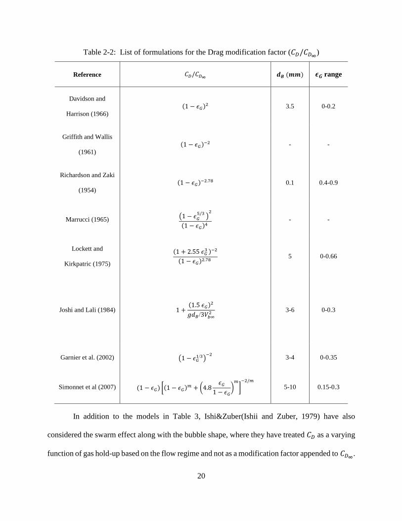
Table 2-2: List of formulations for the Drag modification factor (𝐶𝐷/𝐶𝐷∞)
Reference 𝐶𝐷/𝐶𝐷∞ 𝒅𝑩 (𝒎𝒎) 𝝐𝑮 range
Davidson and
Harrison (1966)
(1 − 𝜖𝐺)2 3.5 0-0.2
Griffith and Wallis
(1961)
(1 − 𝜖𝐺)−2 - -
Richardson and Zaki
(1954)
(1 − 𝜖𝐺)−2.78 0.1 0.4-0.9
Marrucci (1965) (1 − 𝜖𝐺
5/3 )2
(1 − 𝜖𝐺)4
- -
Lockett and
Kirkpatric (1975)
(1 + 2.55 𝜖𝐺3 )−2
(1 − 𝜖𝐺)2.78
5 0-0.66
Joshi and Lali (1984)
1 +(1.5 𝜖𝐺)
2
𝑔𝑑𝐵/3𝑉𝑏∞2 3-6 0-0.3
Garnier et al. (2002) (1 − 𝜖𝐺1/3)
−2 3-4 0-0.35
Simonnet et al (2007) (1 − 𝜖𝐺) [(1 − 𝜖𝐺)𝑚 + (4.8
𝜖𝐺1 − 𝜖𝐺
)𝑚
]−2/𝑚
5-10 0.15-0.3
In addition to the models in Table 3, Ishi&Zuber(Ishii and Zuber, 1979) have also
considered the swarm effect along with the bubble shape, where they have treated 𝐶𝐷 as a varying
function of gas hold-up based on the flow regime and not as a modification factor appended to 𝐶𝐷∞.

21
Figure 2-1 shows the extent of variation in the prediction of the drag modification factor by these
models.
Figure 2-1: Comparison of different formulations for the drag modification factor from Literature

22
2.3.2 Lift force
When there is a velocity gradient lateral to the direction of bubble motion, then bubbles
experience a combination of forces (Magnus effect and Shear effect) in the lateral direction which
is referred to as Lift force (𝐹𝑙𝑖𝑓𝑡). The general formulation for lift force is given by:
𝐹𝑙𝑖𝑓𝑡 = −𝐶𝐿𝜌𝐿𝜖𝐺(𝑣𝐿 − 𝑣𝐺) × (𝛻 × 𝑣𝐿) (2-12)
2.3.3 Virtual mass force
When the flow is decelerating or accelerating, the bubbles experience a Virtual Mass force
(𝐹𝑣𝑚). The following relation was used for calculating the 𝐹𝑣𝑚.
𝐹𝑣𝑚 = 𝜖𝐺𝜌𝐿𝐶𝑣𝑚
𝐷
𝐷𝑡(𝑣𝐿 − 𝑣𝐺) (2-13)
Where 𝐶𝑣𝑚 = 0.5 was used.
2.3.4 Turbulent dispersion force
The turbulent dispersion force quantifies the effect of the liquid eddies in transporting the
bubbles. The formulation of the turbulent dispersion force is based on an analogy to molecular
diffusion. The turbulent dispersion of the gas bubbles, plays a key role in determining the local
hold-up of the gas phase. The expression derived by Lopez de Bertodano (Lopez de Bertodano,
1992) is given as follow:
23
𝐹𝑡𝑑 = −𝐶𝑡𝑑𝜌𝐿𝑘𝛻𝜖𝐺 (2-14)
Where, k is the turbulent kinetic energy and 𝐶𝑡𝑑 is the turbulent dispersion coefficient and 𝐶𝑡𝑑=
0.2 was used.
2.3.5 Wall lubrication force
The Wall lubrication force is used to model the movement of bubbles away from the wall.
𝐹𝑤𝑙 = 𝐶𝑤𝑙𝜌𝐿𝜖𝐿|𝑣𝐿 − 𝑣𝐺|2 𝑛𝑤 (2-15)
Where 𝐶𝑤𝑙 = max (0,𝐶𝑤1
𝑑𝐵+𝐶𝑤2
𝑦𝑤) , 𝐶𝑤1 = −0.01, 𝐶𝑤2 = 0.05

24
Chapter 3. Modelling of a Plunging Jet Bubble Column with Variable Free
Jet Length
Introduction
Typically in bubble columns the gas phase is up flowing and the liquid phase is in batch
mode (semi-batch bubble column) or up-flowing. Whereas, in a down-flow bubble column the
Introduction of both the gas and liquid phase from the top enables inverse bubbly flow where the
bubbles are made to move against their natural tendency to raise up due to buoyancy, thereby much
higher gas-holdups can be achieved. Further, the entrainment of the gas bubbles by the plunging
jet action enables generation of fine bubbles in the micro-bubble range thus creating large
interfacial area. For these reasons plunging jet bubble columns have been used in flotation units in
mineral processing industries (Evans et al., 1992; Mao et al., 1991). Many experimental studies
have been carried out in the past to measure the gas-holdup and absorbance performance of these
columns (Atkinson et al., 2008; Evans et al., 2001b; Ohkawa et al., 1984; Yamagiwa et al., 1990).
The key feature of the plunging jet down-flow bubble column is a plunging liquid jet that
is used to entrain the inlet gas in the column of liquid. Experimental characterization of the
plunging jet and the subsequent gas entrainment has been studied extensively and the physics is
well understood (Kiger and Duncan, 2012; Roy et al., 2013). But still the successful CFD
simulation of the plunging liquid jet, the associated gas entrainment and the resultant two-phase
bubbly dispersion flow in the downstream section; all of these phenomena in a single simulation
still remains a challenge.
Although The existing high resolution CFD models like the Volume Of Fluid (VOF)
method and Front-tracking method have been successfully employed to capture the phenomena
occurring above and below the free-liquid surface (Deshpande et al., 2012; Khezzar et al., 2015;

25
Qu et al., 2011)they are limited in application for cases where the entrained gas bubbles are of few
mm size and further as their computational requirement is very high, these models are not suitable
for full- reactor scale simulations. On the other hand the low resolution model like Eluer-Euler
model has been successfully employed to capture only the phenomena occurring below the free
surface by applying a two-phase bubbly flow inlet with pre-determined jet-velocity profile from
the free surface of the liquid pool (Kendil et al., 2012, 2011; Krepper et al., 2010). This approach
works fine for cases were the tank or container cross-sectional area is sufficiently large and the
free surface sloshing can be neglected.
26
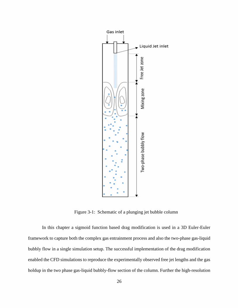
Figure 3-1: Schematic of a plunging jet bubble column
In this chapter a sigmoid function based drag modification is used in a 3D Euler-Euler
framework to capture both the complex gas entrainment process and also the two-phase gas-liquid
bubbly flow in a single simulation setup. The successful implementation of the drag modification
enabled the CFD simulations to reproduce the experimentally observed free jet lengths and the gas
holdup in the two phase gas-liquid bubbly-flow section of the column. Further the high-resolution

27
turbulence and holdup data obtained from the 3D CFD simulations for the different operating
conditions were utilized to perform a linear stability analysis (Ghatage et al., 2014) to determine
the critical gas holdup at which the regime transition from the homogeneous regime to the
heterogeneous regime takes place. The prediction of this critical holdup at which the regime
transition occurs is crucial for the design and scale-up of bubble column reactors.
Experimental data
The experimental conditions for which the CFD simulations and the stability analysis have
been performed is taken from (Evans, 1990). The column under consideration has a diameter of
0.044 m and length of 1m. The liquid jet inlet at the top has a nozzle-diameter of 4.76 mm. The
experimental data consisted of the observed free jet length for the plunging liquid jet, the gas hold-
up in the two-phase bubbly flow region in the bottom section of the column and the mean-diameter
of the bubbles in the micro-bubble dispersion in the bottom section of the column. The
experimental data utilized for the work presented here is for the liquid superficial velocity of VL =
34 mm/s, corresponding to the jet velocity of 11.73 mm/s at the inlet nozzle. The gas superficial
velocity was varied for each operating condition ranging from VG = 6.41 - 49.96 mm/s. Figure
1-2 shows the increase in the free jet length of the plunging liquid jet and the gas hold-up in the
two phase bubbly flow region as the gas superficial velocity VG increases.

28
Figure 3-2: Experimental Gas hold-up and free jet length data from (Evans, 1990) for VL = 34
mm/s and VG = 6.41 - 49.96 mm/s.
CFD setup
The mesh used for the CFD simulations is shown in Figure 1-3. A 3D structured mesh with
a cell count of 0.3 million was used. The jet velocity of 11.73 mm/s corresponding to the liquid
superficial velocity of VL = 34 mm/s was specified as the liquid inlet velocity at the inlet boundary
corresponding to the liquid nozzle. A turbulent intensity of 5% and a hydraulic diameter equal to
the nozzle diameter (4.76 mm) was specified at the liquid inlet. The annular space between the
0
0.05
0.1
0.15
0.2
0.25
0.3
0
0.1
0.2
0.3
0.4
0.5
0.6
0.7
0.8
0.9
0.00 10.00 20.00 30.00 40.00 50.00
Fre
e Je
t le
ng
th (
m)
Gas
ho
ldup
(-)
Superficial gas velocity VG (mm/s)
Gas holdup exp
Jet length
29
nozzle and the column wall at the top of the column was specified as a gas inlet with a local
velocity corresponding to that of the superficial velocity. The column wall and the liquid-nozzle
walls were modelled as a wall boundary with a no-slip condition. A pressure outlet with a constant
gauge pressure of zero was used for the bottom outlet. The flow fields were initialized with a
column fully filled with liquid up to the gas inlet, and then the flow equations corresponding to the
Euler-Euler framework described in Chapter 2 were solved with a constant time step of 0.001s.
The drag-force and virtual mass force were the only two interphase forces considered and the other
interphase forces like the lift force, turbulent dispersion force, wall lubrication force etc. were
neglected. For the drag force, the Schiller Neumann correlation was used, which is only applicable
in the two-phase bubbly flow region. As discussed earlier a drag modification/enhancement factor
is introduced to capture gas entrainment by the plunging action of the liquid jet. The details and
exact implementation of this drag modification function are discussed in the following section. For
the cases with the successful implementation of the drag modification/enhancement factor, fully
developed flow profiles were observed after 15-20s. Once the flow was fully developed after 30s,
the flow field data was time averaged for another 10s. This time averaged data was used for the
subsequent analysis as in the linear stability analysis to determine the critical gas hold-up.

30
Figure 3-3: Computational mesh used for the plunging jet bubble column.
Wall Wall
Gas-Liquid dispersion Outlet
Gas inlet
Liquid jet inlet

31
Sigmoid function based drag modification for capturing the gas entrainment by the
plunging liquid jet
In the Euler-Euler framework the description of the gas phase is treated as a secondary
dispersed phase with a constant bubble diameter through-out the column. Further by default the
drag-laws employed in the Euler-Euler framework are either meant for bubbly-flow or misty-flow
(liquid droplets become the dispersed-secondary phase). But in reality for the plunging jet both the
gas and liquid phase are continuous phases near the inlet in the top section of the column. So
clearly due to the Euler-Euler description, and as the coarse grid employed in this region is not
fine enough to capture the complex interface formation and breakage process, a drag-enhancement
to the existing bubbly flow drag-law is required in this region to ensure the complete entrainment
of the gas-phase in the liquid phase. This drag enhancement is applied by means of a sigmoid
function that varies with the local gas hold-up (Eq.(17)). Without this drag-modification, the CFD
simulations fail to capture the gas entrainment process completely and the column either drains
completely or it produces unrealistic free-jet lengths that are very different from experimental
observations.
𝐹𝑑𝑟𝑎𝑔 =
𝐴𝑖8𝐶𝐷𝜌𝐿 |(𝑣𝐺 − 𝑣𝐿)|(𝑣𝐺 − 𝑣𝐿), 𝑤ℎ𝑒𝑟𝑒 𝐴𝑖 =
6𝜖𝐺(1 − 𝜖𝐺)
𝑑𝐵 (3-1)
Df = Df𝑜 +
Df𝑚𝑎𝑥 − Df𝑜
1 + 𝑒−𝑘(𝜖𝐺−𝜖𝐺𝑐𝑟𝑖𝑡 ) (3-2)

32
Figure 3-4: Variation of the sigmoid function based drag modification factor with gas hold-up.
0
5
10
15
20
25
0 0.2 0.4 0.6 0.8 1
Df
(-)
Fractional gas hold-up, ϵG (-)
Df col1
33
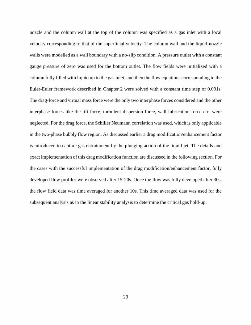
Figure 3-5: Variation of the product of Drag modification factor and the specific interfacial area
calculated using the symmetric method, with gas hold-up.
The parameter Df𝑜 takes into account any constant drag-modification that needs to be
implemented for improving the accuracy of the two-phase bubbly flow in the bottom section of
the column. The parameter Df𝑚𝑎𝑥 fixes the maximum value or plateau reached by the sigmoid
function. The exponent k determines the sharpness of this transition and 𝜖𝐺𝑐𝑟𝑖𝑡 determines the gas
hold-up around which this transition is activated typically between 0.7 - 0.9, as expected in the
free-jet region. The optimum values of these parameters were obtained by considering different
profiles of ‘ai*Df’ as a function of the local gas holdup as shown, these profiles correspond to the
different sets of parameters as listed in Table 1-1.
0E+0
1E+4
2E+4
3E+4
4E+4
5E+4
6E+4
0 0.2 0.4 0.6 0.8 1
Df*
a i (
m-1
)
Fractional gas hold-up, ϵG (-)
ai*Df_3
ai
ai * Df

34
.
Figure 3-6: Comparison of Df for different sets of parameters
0.0E+0
2.0E+4
4.0E+4
6.0E+4
8.0E+4
1.0E+5
1.2E+5
1.4E+5
1.6E+5
0 0.2 0.4 0.6 0.8 1
Df*
a i
Fractional gas hold-up (-)
ai*Df_1
ai*Df_2
ai*Df_3
ai*Df_4
ai*Df_5
ai*Df_6
ai*Df_7
ai*Df_8
ai*Df_9
ai*Df_10
ai*Df_11
ai*Df_12
ai*Df_13

35
Table 3-1 Values of different sets of parameters considered for Df
Set No. Df𝒐 Df𝒎𝒂𝒙 𝒌 𝝐𝑮𝒄𝒓𝒊𝒕
1 1.5 20 20 0.65
2 1 30 18 0.75
3 1 24 50 0.75
4 1 35 40 0.75
5 0.5 50 20 0.75
6 0.5 50 20 0.7
7 0.75 60 30 0.7
8 0.5 100 25 0.8
9 1 95 15 0.77
10 1 60 40 0.75
11 1 18 60 0.75
12 1 15 40 0.75
13 1 15 20 0.75
The Drag modification function was implemented using Fluent User Defined Funciton
(UDF) and the C code is provided in the appendix A. Of the 15 data points corresponding to each
operating condition determined by the gas superficial velocities VG, 5 data points corresponding
to VG = 9.45, 23.62, 32.36 and 38.47 mm/s were used as training data to obtain the optimum values
for the parameters (Df𝒐, Df
𝒎𝒂𝒙, 𝒌, 𝝐𝑮𝒄𝒓𝒊𝒕) by matching the free jet lengths observed from CFD to
that of the experimental values. The values corresponding to set-3 in Table 1-1 were found to give

36
the closest values of the free jet lengths from the CFD to that of the experimental values. Figure
1-7 shows the comparison of the free jet length values obtained from CFD simulations using the
optimum values for the parameters (set-3) in the drag modification function Df . Without the
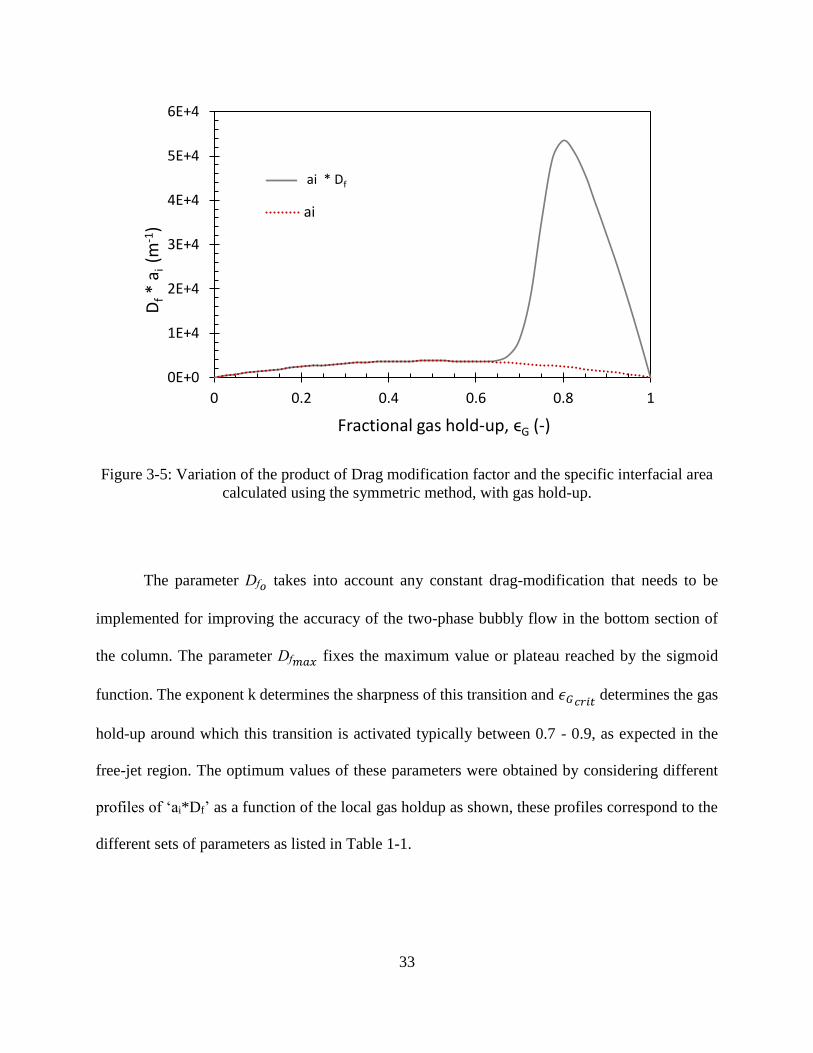
implementation of this drag-modification, the CFD simulations fail to capture the gas entrainment
process and as the simulation proceeds the column is completely drained. This is shown in Figure
1-8 , where it can be observed that without the necessary local drag enhancement the liquid jet
fails to entrain the gas from the bulk-phase and this results in continuously increasing liquid jet
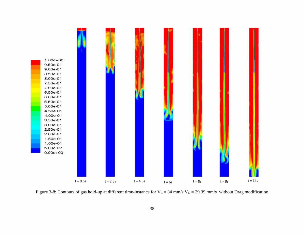
length as the simulation proceeds and eventually the column is completely drained. Figure 1-9
shows the effect of incorporating the drag modification enabling the CFD simulations to capture
the entrainment process more reliably, which in turn enables the simulation of the resultant two-
phase bubbly flow in the bottom section of the column.

37
Figure 3-7: Comparison of Free jet length values obtained from CFD with the experimental
values
0
0.05
0.1
0.15
0.2
0.25
0.3
0 0.05 0.1 0.15 0.2 0.25 0.3
Fre
e je
t le
ng
th f
rom
CF
D (
m)
Free jet length from Experiments (m)
Training_data
test data
+0.05 m
- 0.05 m
38
Figure 3-8: Contours of gas hold-up at different time-instance for VL = 34 mm/s VG = 29.39 mm/s without Drag modification
t = 0.5s t = 2.5s t = 4.5s t = 6s t = 8s t = 9s t = 14s
39
Figure 3-9: Contours of gas hold-up at different time-instance VL = 34 mm/s VG = 29.39 mm/s with Drag modification
t = 0.5s t = 2.5s t = 4.5s t = 6s t = 8s t = 9s t = 14s

40
CFD results
The average gas hold-up in the bubbly flow section was computed by volume averaging
the gas hold-up field for a column length of 20 cm just above the column exit. These values are
compared with the experimentally observed average gas hold-up in Figure 3-10. Although the CFD
Figure 3-10: Comparison of the average gas hold-up in the two-phase bubbly flow region from
CFD with the experimental values
The contours of the time averaged gas hold-up for the different gas superficial velocities
VG are given in . It can be observed that the implementation of the drag modification function has
enabled the CFD simulations to successfully capture all the three zones: 1) the free-liquid jet, 2)
The mixing zone, and 3) the two-phase bubble flow region.
0
0.1
0.2
0.3
0.4
0.5
0.6
0.7
0.8
0.9
0 10 20 30 40 50
Gas
ho
ldup
(-)
Superficial gas velocity VG (mm/s)
Exp
CFD

41
Figure 3-11: Contours of time averaged gas hold-up for different gas superficial velocities VG.
42
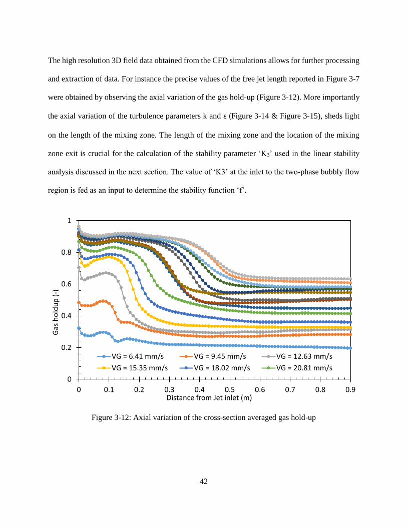
The high resolution 3D field data obtained from the CFD simulations allows for further processing
and extraction of data. For instance the precise values of the free jet length reported in Figure 3-7
were obtained by observing the axial variation of the gas hold-up (Figure 3-12). More importantly
the axial variation of the turbulence parameters k and ԑ (Figure 3-14 & Figure 3-15), sheds light
on the length of the mixing zone. The length of the mixing zone and the location of the mixing
zone exit is crucial for the calculation of the stability parameter ‘K3’ used in the linear stability
analysis discussed in the next section. The value of ‘K3’ at the inlet to the two-phase bubbly flow
region is fed as an input to determine the stability function ‘f’.
Figure 3-12: Axial variation of the cross-section averaged gas hold-up
0
0.2
0.4
0.6
0.8
1
0 0.1 0.2 0.3 0.4 0.5 0.6 0.7 0.8 0.9
Gas
ho
ldu
p (
-)
Distance from Jet inlet (m)
VG = 6.41 mm/s VG = 9.45 mm/s VG = 12.63 mm/s
VG = 15.35 mm/s VG = 18.02 mm/s VG = 20.81 mm/s

43
Figure 3-13: Free Jet lengths obtained from analyzing the axial profiles of gas hold-up
0
0.05
0.1
0.15
0.2
0.25
0.3
0 10 20 30 40 50 60
Fre
e Je
t le
ng
th (
m)
Superficial gas velocity VG (mm/s)
Exp
CFD

44
Figure 3-14: Axial variation of the cross-section averaged turbulent kinetic energy k
0
0.2
0.4
0.6
0.8
1
0 0.1 0.2 0.3 0.4 0.5 0.6 0.7 0.8
k (
m2/s
2)
Distance from Jet inlet (m)
VG = 6.41 mm/sVG = 9.45 mm/sVG = 12.63 mm/sVG = 15.35 mm/sVG = 18.02 mm/sVG = 20.81 mm/sVG = 23.62 mm/sVG = 26.44 mm/sVG = 29.4 mm/sVG = 32.36 mm/sVG = 35.42 mm/sVG = 38.47 mm/sVG = 41.98 mm/sVG = 46.65 mm/s

45
Figure 3-15: Axial variation of the cross-section averaged turbulent dissipation rate є
Linear stability analysis
One of the main motivations to pursue a CFD analysis is to obtain 3D high resolution flow
field data, that provides better insight into the local flow circulations and more importantly it gives
a better picture of the local variations in the turbulence quantities like the turbulent kinetic energy
k and turbulent energy dissipation rate ԑ. In this section we demonstrate the utility of such a high
resolution 3D field data for performing a linear stability analysis to obtain the critical gas holdup
at which regime transition from the homogeneous regime to the heterogeneous regime takes place.
Linear stability analysis for multiphase flows, involves introduction of a small perturbation
in the continuity and momentum equations (Anderson and Jackson, 1969; Bhole and Joshi, 2005;
Ghatage et al., 2014; Joshi et al., 2001). In this chapter we utilize the stability function ‘f1’ as
0
20
40
60
80
100
0 0.1 0.2 0.3 0.4 0.5 0.6 0.7
ԑ(m
2/s
3)
Distance from Jet inlet (m)
VG = 6.41 mm/sVG = 9.45 mm/sVG = 12.63 mm/sVG = 15.35 mm/sVG = 18.02 mm/sVG = 20.81 mm/sVG = 23.62 mm/sVG = 26.44 mm/sVG = 29.4 mm/sVG = 32.36 mm/sVG = 35.42 mm/sVG = 38.47 mm/sVG = 41.98 mm/sVG = 46.65 mm/s

46
proposed by (Joshi et al., 2001). The stability criterion for transition from homogeneous to
heterogeneous flow is given by ‘f1 = 0’. Here the stability function is defined in equation
𝑓1 = 1 − [𝐴 (
𝐺𝐹) −
𝐵2]
2
𝐴(𝑍 − 𝐶) +𝐵2
4
(3-3)
Where, the parameters A, B, C, F, G and Z are defined as:
𝐴 = 𝜌𝐺𝐾0(1 − 𝜖𝐺 )
2+𝜌𝐿𝐾0(1 − 𝜖𝐺)+𝜌𝐿𝐶𝑉0(1 + 2𝜖𝐺) − 𝜌𝐿𝐾0(1 − 𝜖𝐺)2
𝜌𝐿𝐾0(1 − 𝜖𝐺)2
(3-4)
𝐵 = 2𝜌𝐺𝐾0𝑉𝐺(1 − 𝜖𝐺)
3 + 2𝜌𝐿𝑉𝐺𝐶𝑉0(1 + 2𝜖𝐺)(1 − 𝜖𝐺)2 + 2𝜌𝐿𝐾0𝑉𝐿𝜖𝐺
2(1 − 𝜖𝐺)
𝜌𝐿𝐾0𝜖𝐺(1 − 𝜖𝐺)3
+ [2𝜌𝐿𝐶𝑉0𝑉𝐿𝜖𝐺
2(1 + 2𝜖𝐺)
𝜌𝐿𝐾0𝜖𝐺(1 − 𝜖𝐺)3]
(3-5)
𝐶 = 𝜌𝐺𝐾0𝑉𝐺
2(1 − 𝜖𝐺 )4+ 𝜌𝐿𝐶𝑉0𝑉𝐺
2(1 + 2𝜖𝐺)(1 − 𝜖𝐺)3 + 𝜌𝐿𝐾0𝑉𝐿
2𝜖𝐺3(1 − 𝜖𝐺)
𝜌𝐿𝐾0𝜖𝐺2(1 − 𝜖𝐺)4
(3-6)
𝐹 = 𝑔𝑧𝜖𝐺(𝜌𝐺 − 𝜌𝐿)
𝜌𝐿[𝑉𝐺(1 − 𝜖𝐺) − 𝑉𝐿𝜖𝐺]
(3-7)
𝐺 = 𝑔𝑧(𝜌𝐺 − 𝜌𝐿)[𝑉𝐺(1 − 𝜖𝐺)
2 + 𝑉𝐿𝜖𝐺2]
𝜌𝐿(1 − 𝜖𝐺)[𝑉𝐺(1 − 𝜖𝐺) − 𝑉𝐿𝜖𝐺]
(3-8)

47
𝑍 = 𝑔𝑧𝐾2𝑑𝐵|𝑉𝐺(1 − 𝜖𝐺) + 𝑉𝐿𝜖𝐺]
𝐾0(1 − 𝜖𝐺)3[𝑉𝐺(1 − 𝜖𝐺) − 𝑉𝐿𝜖𝐺] ∗
[𝐾0𝜖𝐺(1 − 𝜖𝐺)3 + 𝐶𝑉0(1 − 𝐾3)𝜖𝐺
3(1 + 2𝜖𝐺) + 𝐾0𝐾3𝜖𝐺2(1 − 𝜖𝐺
2)]
(3-9)
Where,
𝐶𝑉 = 𝐶𝑉0 (3 − 2(1 − 𝜖𝐺)
𝐾0(1 − 𝜖𝐺)) (3-10)
𝐶𝑉0 = 0.5 + 𝐾1 ∗ 𝑇𝑎 (3-11)
Typical values used for 𝐾0, 𝐾1, 𝐾2 are 1, 0.143 and 3 respectively.
3.6.1 Stability parameter K3
The stability parameter K3 in equation (3-9) is defined as the ratio of the fluctuating liquid
velocity (𝑢′𝑙) to the fluctuating gas velocity (𝑢′𝑔), at the inlet to the two-phase bubbly flow region.
𝐾3 = (𝑢′𝐿𝑢′𝐺
)𝑖𝑛𝑙𝑒𝑡
(3-12)
It is to be noted that the fluctuating liquid velocity is given by the square root of the turbulent
kinetic energy ‘k’.
𝑢′𝐿𝑖𝑛𝑙𝑒𝑡 = √𝑘𝑖𝑛𝑙𝑒𝑡 (3-13)
And also, the fluctuation gas velocity at any given axial location is given as (Joshi et al., 2001)

48
𝑢′𝐺 = 𝜖𝐺(𝑉𝐿 − 𝑉𝐺) (3-14)
Thus the value of K3 depends on the turbulence generation mechanism or the extent of
liquid phase turbulence at the inlet to the two-phase flow region. Usually for plunging jet bubble
columns it is treated as a complex function of the jet properties like the jet velocity and jet diameter.
In the presented work, the turbulence field data is used to locate the exact location of the inlet to
the two-phase flow region, and further the values of turbulent kinetic energy ‘k’ and gas holdup
‘𝜖𝐺’ is utilized to find an estimate of the value of K3 at the mixing zone exit.
𝐾3 = [√𝑘𝑖𝑛𝑙𝑒𝑡
𝜖𝐺(𝑉𝐿 − 𝑉𝐺)]mixing zone exit
(3-15)
From the axial profiles of the turbulent kinetic energy ‘k’ (Figure 3-14) it can be observed
that it reaches a maximum value at the center of the mixing-zone region and then settles back to a
baseline value, indicating the end of the mixing zone (MZ exit) and the start of the two-phase
bubbly flow region. Previously it was indicated that the length of the free jet or the starting location
of the mixing zone can be obtained from the axial profiles of the gas hold-up (Figure 3-12). So it
can be inferred from Figure 3-16, that the length of the mixing zone increases as the gas injection
rate increases.

49
Figure 3-16: Axial location of the Mixing zone obtained from the axial profiles of the gas hold-
up (Mixing zone entrance) and the turbulent kinetic energy (Mixing zone exit)
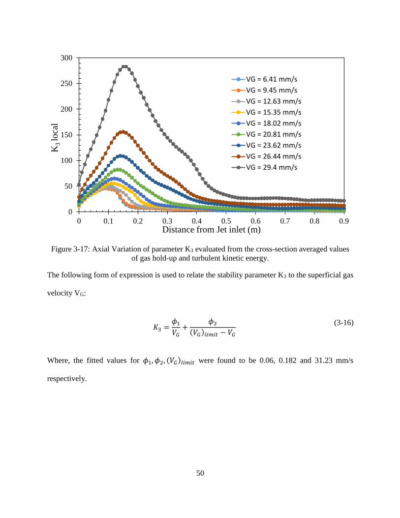
The axial variation of K3 evaluated from the local values of gas hold-up and turbulent
kinetic energy for the different operating conditions is given in Figure 3-17. For determining the
stability function ‘f1’ given by equation (3-3), K3 needs to be expressed as a continuous function
of the operating conditions, i.e. as a continuous function of gas superficial velocity VG as the liquid
superficial velocity VL has been fixed as a constant for this study.
0
0.1
0.2
0.3
0.4
0.5
0.6
0 10 20 30 40 50 60
Axi
al lo
cati
on
fro
m je
t in
let
(m)
Superficial gas velocity VG (mm/s)
Mixing Zone exit
Mixing Zone entrance
50
Figure 3-17: Axial Variation of parameter K3 evaluated from the cross-section averaged values
of gas hold-up and turbulent kinetic energy.
The following form of expression is used to relate the stability parameter K3 to the superficial gas
velocity VG:
𝐾3 =𝜙1𝑉𝐺+
𝜙2(𝑉𝐺)𝑙𝑖𝑚𝑖𝑡 − 𝑉𝐺
(3-16)
Where, the fitted values for 𝜙1, 𝜙2, (𝑉𝐺)𝑙𝑖𝑚𝑖𝑡 were found to be 0.06, 0.182 and 31.23 mm/s
respectively.
0
50
100
150
200
250
300
0 0.1 0.2 0.3 0.4 0.5 0.6 0.7 0.8 0.9
K3 lo
cal
Distance from Jet inlet (m)
VG = 6.41 mm/s
VG = 9.45 mm/s
VG = 12.63 mm/s
VG = 15.35 mm/s
VG = 18.02 mm/s
VG = 20.81 mm/s
VG = 23.62 mm/s
VG = 26.44 mm/s
VG = 29.4 mm/s

51
Figure 3-18: Curve fitting for the K3 values obtained from the CFD analysis.
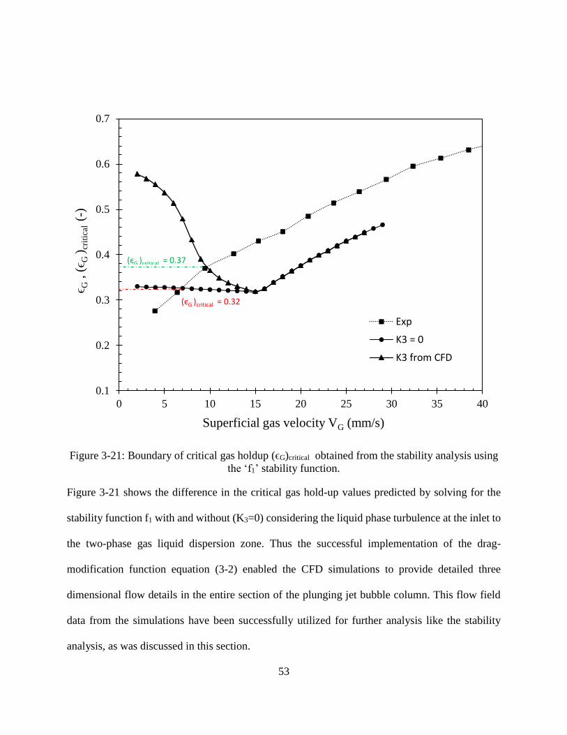
3.6.2 Critical gas hold-up
By incorporating the expression for the stability parameter K3 given by (3-16) in the
expression for the stability function ‘f1’ (3-3), allows for mapping f1 against the gas-holdup 𝜖𝐺 for
each one of the operating conditions (VG ). The first root of f1 (𝜖𝐺 value at which f1 crosses the x-
axis), gives the critical holdup value (ϵG)critical for that operating condition as predicted by the
stability analysis. Figure 3-19 and Figure 3-20 shows the variation of the stability function f1 with
respect to gas holdup for different operating conditions VG = 3.9 mm/s and VG = 29.4 mm/s
respectively. By repeating this procedure for each one of the operating condition a corresponding
transition or critical gas holdup (ϵG)critical can be determined. The mapping of this critical gas
holdup as a function of the operating condition VG yields in a critical gas holdup front, as shown
in Figure 3-21.
0
20
40
60
80
100
120
140
160
0 5 10 15 20 25 30
K3
at M
ixin
g z
on
e ex
it (
-)
VG (mm/s)
K3 MZ exit (CFD)
curve fit

52
Figure 3-19: Stability function f1 as a function of gas holdup ϵG for operating condition of VG =
3.9 mm/s
s
Figure 3-20: Stability function f1 as a function of gas holdup ϵG for operating condition of VG
= 29.4 mm/s
-4
-2
0
2
4
0 0.1 0.2 0.3 0.4 0.5 0.6 0.7 0.8
f1 (
-)
Gas holdup ϵG (-)
(ϵG)critical = 0.34
-4
-2
0
2
4
0 0.1 0.2 0.3 0.4 0.5 0.6 0.7 0.8
f1 (
-)
Gas holdup ϵG (-)
(ϵG)critical = 0.474
53
Figure 3-21: Boundary of critical gas holdup (ϵG)critical obtained from the stability analysis using
the ‘f1’ stability function.
Figure 3-21 shows the difference in the critical gas hold-up values predicted by solving for the
stability function f1 with and without (K3=0) considering the liquid phase turbulence at the inlet to
the two-phase gas liquid dispersion zone. Thus the successful implementation of the drag-
modification function equation (3-2) enabled the CFD simulations to provide detailed three
dimensional flow details in the entire section of the plunging jet bubble column. This flow field
data from the simulations have been successfully utilized for further analysis like the stability
analysis, as was discussed in this section.
0.1
0.2
0.3
0.4
0.5
0.6
0.7
0 5 10 15 20 25 30 35 40
ϵ G, (ϵ
G )
crit
ical
(-
)
Superficial gas velocity VG (mm/s)
Exp
K3 = 0
K3 from CFD
(ϵG )critical = 0.37
(ϵG )critical = 0.32

54
Conclusions
In this chapter we reviewed the current experimental studies and modelling approaches
used for understanding the flow behavior in a down-flow plunging liquid jet bubble column. The
need for implementing a drag modification function in the Euler-Euler framework to capture the
gas-entraining action of the plunging liquid jet to create the two-phase gas-liquid dispersion was
highlighted. To achieve the same, a sigmoid function based drag modification function was
proposed and the values of the parameters involved in it were obtained by performing a tuning
procedure that involved matching the free jet lengths obtained from the CFD simulations with that
of the experimentally observed values. The tuned drag modification function was capable of
reliably capturing the plunging jet action for all the operating conditions, and this enabled the CFD
simulations to capture the flow details involved in all three zones of the plunging jet bubble
column. Further, the three dimensional velocity and turbulence data obtained from the CFD
simulations were put to use for performing a linear stability analysis to determine the critical gas
holdup at which the regime transition from homogeneous to heterogeneous regime takes place.

55
Chapter 4. CFD-PBM Modelling of a Novel Down Flow Bubble Column
Introduction
This chapter deals with the flow modelling for a novel down-flow bubble column
incorporating the micro-bubble generation mechanism using an array of liquid jets as discussed in
section 1.2. The CFD simulations have been setup to capture the flow conditions studied
experimentally by (Hernandez-Alvarado et al., 2017a). Conventionally in the simulation of bubbly
flows in the Euler-Euler framework as in the previous chapter, a constant bubble diameter is used
for the description of the dispersed gas phase. This value of the bubble diameter is a crucial input
for evaluating all the inter-face forces most importantly the drag force. This bubble diameter is
treated as a constant for the entire computational domain and it also remains constant as the
transient simulation progresses in time. This is remedied by coupling a Population Balance Model
(PBM) with the Euler-Euler equations (Buwa and Ranade, 2002; Lehr et al., 2002; Lo, 1996a;
Olmos et al., 2001), the PBM equations keeps track of the spatial and time evolution of the bubble
size distribution. Then a Sauter-mean diameter that is calculated from this spatially and temporally
varying bubble size distribution is utilized to evaluate the inter-facial forces. This chapter deals
with the use of a discrete implementation of CFD-PBM. We briefly the discuss the experimental
setup and data for which the modelling is performed, then we discuss the Discrete PBM method
and the CFD-PBM coupling, later we discuss the CFD-PBM setup and some of the results for the
flow conditions encountered in this novel down-flow bubble column.
Experimental setup and data
The experimental setup of the down-flow column is shown in Figure 4-1. The acrylic
column has a diameter of 0.1m and a height of 0.6m. The orifice plate used for generating the array
of liquid jets at the top has orifices of 400 µm diameter arranged in a triangular pitch of 3mm. A

56
three arm gas sparger with four 1mm holes on each arm is used to inject the mm sized large bubbles
from the bottom. A surfactant additive of 10 ppm SDS (Sodium dodecyl Sulfate) was added to the
liquid phase to inhibit the coalescence of the micro-bubbles. The column is capable of achieving
stable down-flow conditions for the superficial velocities in the range of VL=40-80 mm/s and
VG=2-20 mm/s.
Figure 4-1: Image of the novel down-flow bubble column of 10 cm diameter: (a) Column with
header section and orifice plate between flanges (b) Orifice plate (c) Three-arm gas sparger.
The initial injection of the dispersed phase (gas) through the sparger produces bubbles of
the order of few mms. The injected large bubbles then rise up to the top of the column (jet region)

57
and due to the high kinetic energy of the jets they get broken down to form a fine dispersion of
microbubbles. This gas liquid dispersion consisting of microbubbles then exits the column from
the bottom outlet. Pressure sensors at regular intervals are used to monitor the axial pressure
gradient. The radial gas holdup distribution across a cross section is measured by means of a Wire
Mesh Sensor system, and also by Gamma Ray Densitometry. The bubble size distribution is
measured using images of the bubbles captured by a boroscope. Further the RTD of the liquid
phase in the columns is obtained by salt tracer method using conductivity probes. The mass transfer
rate Kl ai is measured from dissolved oxygen sensors at the inlet and outlet of the columns. The
key experimental data are summarized in Table 4-1.
Table 4-1: Eperimental data obtained for different superficial velocities from small rig with
sparger at the bottom, for SDS=25ppm and KCl=75ppm.
VG VL Gas
holdup
Micro-Bubble
Diameter
Interfacial
area Kl *ai
mm/s mm/s % µm m2/m3 hr-1
2.06 78 6.3 253 1490 400.00
2.06 93 2.0 162 741 350.00
6.17 78 14.6 211 4162 1900.00
6.17 93 13.7 192 4276 1300.00
10.3 78 25.6 201 7647 5000.00
10.3 93 20.4 179 6827 4000.00

58
Population balance model (PBM)
Different formulations of population balance models exist, they can be broadly divided into the
Discrete/Multiple Size Group (MUSIG) method and the Method of Moments (MOM). In the
Discrete method, the size distribution is tracked by estimating the number density of bubbles of
each bin/size-group (where the number of bins and the bubble size for each bin is preset), by
solving a population balance equation (4-1) for each bin. So, the total number of PBM equations
solved is equal to the number of bins, and more the number of bins more accurate is the
representation of the size distribution. This type of PBM coupled with CFD, was first used by (Lo,
1996b) to estimate the bubble size distribution from the coalescence and breakage phenomena.
𝜕
𝜕𝑡(𝛼𝑘𝜌𝑘𝑓𝑖) + 𝛻. (𝛼𝑘𝜌𝑘�⃗�𝑘𝑓𝑖) = 𝜌𝑘𝑆𝑖 (4-1)
Where, equation (4-1) represents the set of population balance equations solved to determine the
bin fraction 𝑓𝑖 for each bin/size-group. The bin fraction 𝑓𝑖 is related to the bubble number density
𝑛𝑖 of that particular bin by:
𝛼𝑘 𝑓𝑖 = 𝑛𝑖 𝑉𝑖 (4-2)
Where 𝑉𝑖 is the volume of a bubble in the ith bin.By considering M size-groups or bins for the gas
phase, and solving the M population balance equations, a size distribution is obtained in each
computational cell, this size distribution is then used to determine a Sauter-mean diameter D32.
𝐷32 = (
∑ 𝑛𝑖 𝐷𝑖3𝑀
𝑖=1
∑ 𝑛𝑖𝐷𝑖2𝑀
𝑖=1
) (4-3)
59
Where, 𝑛𝑖 is the bubble number density in the size-group 𝑖. The interfacial forces (Drag, lift
etc.) and the interfacial area are computed based on D32 from equation (4-3) instead of a constant
bubble diameter that is used in the conventional Euler-Euler framework. Further the term 𝑆𝑖 in
equation (4-1) is the source term for the ith bin due to coalescence and breakage of bubbles and is
defined as
𝑆𝑖 = 𝐵𝐵 + 𝐵𝑐 − 𝐷𝐵 − 𝐷𝐶 (4-4)
Where B and D denotes the source (birth) and sink (death) terms, and the subscript B and C indicate
the breakage or coalescence phenomena causing the birth or death of bubbles. The terms
𝐵𝐵, 𝐵𝑐, 𝐷𝐵, 𝐷𝐶 are in turn calculated based on the choice of breakage and coalescence
kernels/models.
It is to be noted that although the bubbles from each size-group may have different velocities, it is
assumed that they all move with the same velocity. This assumption greatly reduces the
computational demand, as the former requires solving for separate momentum equations for each
size-group of bubbles, which is computationally expensive. As a reasonable remedy to this
approximation of equal velocity for different size-groups of bubbles, bins are further grouped into
velocity groups (Frank et al., 2005). Since a separate momentum balance equation is solved for
each velocity group, this is essentially a multi-fluid approach. This method is now referred to as
‘Inhomogeneous-Discrete’, and the earlier Discrete PBM formulation (Lo, 1996b) is now referred
to as ‘Homogeneous-Discrete’. In our case due to distinct difference in the size distribution of the
injected large bubbles and the micro bubbles generated from the impact of jets with the large
bubbles, the Inhomogeneous-Discrete method is more fitting for our purposes than the
homogenous-Discrete method. Further it is to be noted, that the interfacial forces (Drag)

60
experienced by the large bubbles and micro bubbles are significantly different and hence the
resulting slip velocities experienced by them. For this reason it is more reasonable to treat the large
and micro bubbles as two separate phases. Now this leads to a 3-phase Eulerian-Eulerian
framework consisting of three sets of mass and momentum balance equations being solved for the
three phases. In addition to this the PBM consisting of M bins/size-groups is used for each of the
two dispersed phase (large bubbles and micro bubbles) in the 3 phases. The second class of PBMs
(MOM & QMOM) involves tracking of the statistical-moments, and it involves solving the
moment transport equation for each order of moments that are being solved for. It also involves
the reconstruction of the size distribution from the moments at each time step. The Discrete-PBM
described earlier is used for the work presented in this report. Readers interested in the MOM and
Quadrature based MOM (QMOM) are requested to refer to (Marchisio and Fox, 2013)
PBM kernels:
The coalescence and breakage phenomena are in turn modelled by theoretical and semi-
empirical models referred to as breakage/coalescence kernels. The formulation of the source and
sink terms in the bin fraction equation 𝐵𝐵, 𝐵𝑐, 𝐷𝐵 𝑎𝑛𝑑 𝐷𝐶 ; in turn depends on the choice of the
coalescence and breakage kernels. Some of the commonly used coalescence kernels are: (Luo,
1993; Luo and Svendsen, 1996; Saffman and Turner, 1956). And some of the commonly used
breakage kernels are: (Lehr et al., 2002; Luo and Svendsen, 1996). The broth used in the actual
bio-reactors at Lanzatech, have been tested and confirmed to show a strong non-coalescing
behavior. Also, care was taken for the experiments conducted at CCNY to make the gas-liquid
system to exhibit non-coalescing behavior by the addition of 10 ppm SDS and 75 ppm KCl to
modify the gas-liquid interface properties, that leads to inhibition of coalescence of bubbles. For

61
these reasons, it was decided to drop the coalescence modelling and hence the associated source
and sink terms (𝐵𝑐, 𝐷𝐶) from the PBM formulation.
4.4.1 Breakage kernel
The source and sink terms BB and DB (birth and death of bubbles due to breakage) in
equation (4-4) are functions of the breakage kernel and are intern given by the following
expressions:
𝐵𝐵 = ∑ 𝛺(𝑉𝑗: 𝑉𝑖) 𝑛𝑗
𝑁
𝑗=𝑖+1
(4-5)
𝐷𝐵 = 𝛺𝑖 𝑛𝑖 , 𝑤ℎ𝑒𝑟𝑒 𝛺𝑖 = ∑𝛺𝑖𝑘
𝑁
𝑘=1
(4-6)
Where, 𝛺(𝑉𝑗: 𝑉𝑖) is the breakage rate of bubbles of volume Vj to Vi, and is given by the breakage
kernel. In the present work the Lehr model (Lehr et al., 2002), equation (4-7) is used for the
breakage kernel. The only input parameter for this breakage kernel is the critical Weber
number 𝑊𝑒𝑐𝑟𝑖𝑡, and is used as one of the tuning parameters for our purpose of matching the bubble
size predictions from the CFD-PBM model with the reported values of bubble size measurement.
In equation (4-7), 𝜉 = 𝜆/𝑑𝑗 is the ratio of the length scale of an eddy to the bubble diameter in the
inertial subrange.
𝛺𝑏𝑟(𝑉𝑗: 𝑉𝑖) = 𝐾∫
(1 + 𝜉 )2
𝜉133
𝑒𝑥𝑝 (−𝑏 𝜉−23) 𝑑𝜉
1
𝜉𝑚𝑖𝑛
(4-7)
Where: 𝐾 = 1.19 𝜖−
1
3 𝑑−7
3 𝜎 𝜌−1𝑓−1
3 , 𝑏 = 𝑊𝑒𝑐𝑟𝑖𝑡 𝜎 𝜌−1𝜖−
2
3 𝑑−5
3 𝑓−1
3 .
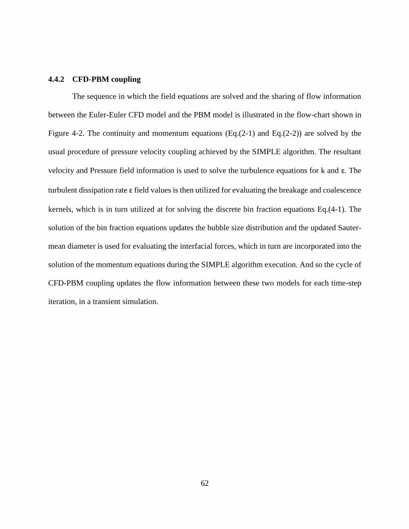
62
4.4.2 CFD-PBM coupling
The sequence in which the field equations are solved and the sharing of flow information
between the Euler-Euler CFD model and the PBM model is illustrated in the flow-chart shown in
Figure 4-2. The continuity and momentum equations (Eq.(2-1) and Eq.(2-2)) are solved by the
usual procedure of pressure velocity coupling achieved by the SIMPLE algorithm. The resultant
velocity and Pressure field information is used to solve the turbulence equations for k and ԑ. The
turbulent dissipation rate ԑ field values is then utilized for evaluating the breakage and coalescence
kernels, which is in turn utilized at for solving the discrete bin fraction equations Eq.(4-1). The
solution of the bin fraction equations updates the bubble size distribution and the updated Sauter-
mean diameter is used for evaluating the interfacial forces, which in turn are incorporated into the
solution of the momentum equations during the SIMPLE algorithm execution. And so the cycle of
CFD-PBM coupling updates the flow information between these two models for each time-step
iteration, in a transient simulation.
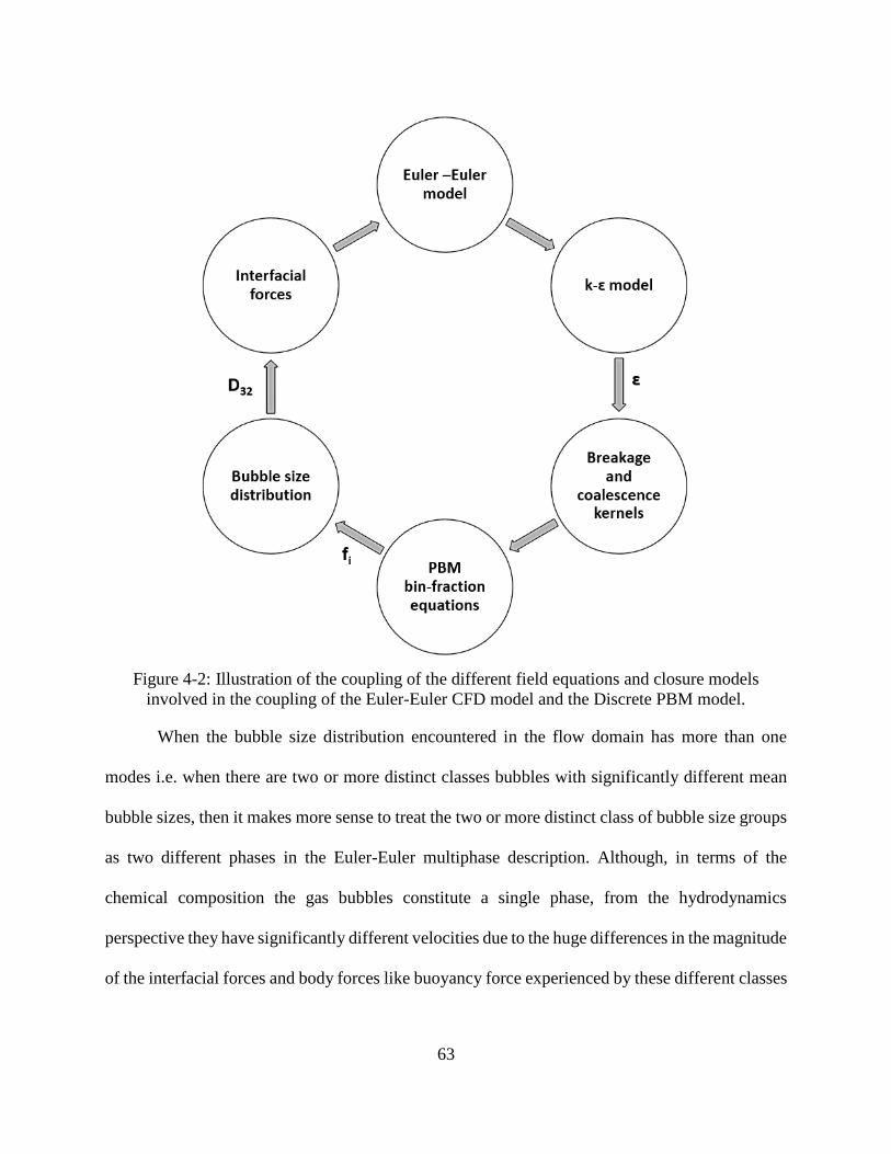
63
Figure 4-2: Illustration of the coupling of the different field equations and closure models
involved in the coupling of the Euler-Euler CFD model and the Discrete PBM model.
When the bubble size distribution encountered in the flow domain has more than one
modes i.e. when there are two or more distinct classes bubbles with significantly different mean
bubble sizes, then it makes more sense to treat the two or more distinct class of bubble size groups
as two different phases in the Euler-Euler multiphase description. Although, in terms of the
chemical composition the gas bubbles constitute a single phase, from the hydrodynamics
perspective they have significantly different velocities due to the huge differences in the magnitude
of the interfacial forces and body forces like buoyancy force experienced by these different classes

64
of bubble size groups. So, this method of further grouping the size-groups/ bins as separate phases
and solving a separate momentum equation for each one of these phases is known as the
inhomogeneous discrete method of PBM. Figure 4-3 shows the difference in the representation of
the bins for a same size distribution by the homogeneous and in-homogeneous discrete methods.
By treating the gas phase as two separate phases one made of mm sized large bubbles and another
consisting micron sized micro-bubbles, the separate evaluation of two different Sauter-mean
diameters is more representative of the bubble size distributions. Further, most importantly the in-
homogenous discreet model allows for capturing the upward motion of large bubbles and
downward motion of micro-bubbles in the same computational cell, which is expected to happen
in the jet region.
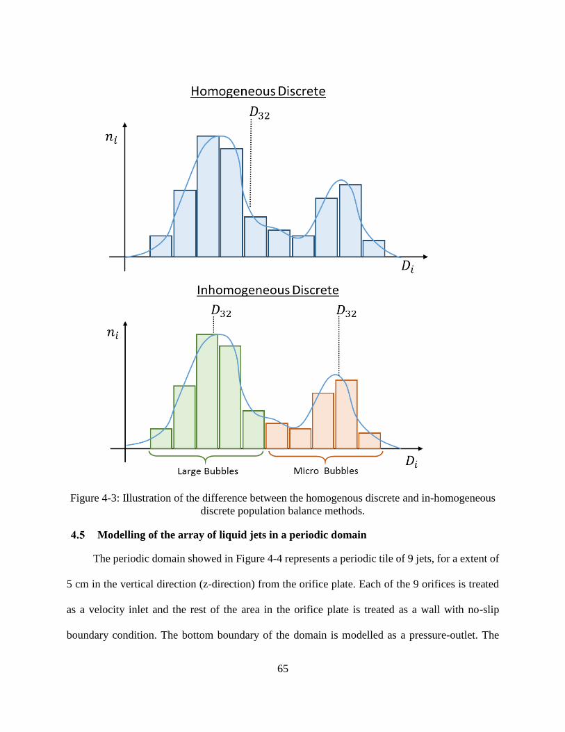
65
Figure 4-3: Illustration of the difference between the homogenous discrete and in-homogeneous
discrete population balance methods.
Modelling of the array of liquid jets in a periodic domain
The periodic domain showed in Figure 4-4 represents a periodic tile of 9 jets, for a extent of
5 cm in the vertical direction (z-direction) from the orifice plate. Each of the 9 orifices is treated
as a velocity inlet and the rest of the area in the orifice plate is treated as a wall with no-slip
boundary condition. The bottom boundary of the domain is modelled as a pressure-outlet. The

66
boundaries defining the limits in the x and y direction are treated as periodic, and this imposes the
periodicity in the x and y directions. This also ensures that the effect of the neighboring jets is
captured. The Jet dynamics and their effectiveness in breaking down the large bubbles to create
micro-bubbles can be studied using the simulations performed in this periodic domain. Each of the
9 orifices through which the liquid is injected is resolved to a sufficient extent to reliably capture
the flow field and the associated turbulence field created by the formation of the jets. The gas phase
was treated as two different phases, one phase consisting of large bubbles ranging in size from
10mm to 1.6mm bubble diameter, and another phase of small bubbles/ micro bubbles ranging in
size from 0.8mm to 70 𝜇m. The exact bin sizes used for the two gas phases is given in
Figure 4-4: Mesh used for modelling the jets created by the orifice plate in a periodic domain.

67
Table 4-2: bin sizes (size-groups) used for the Indiscreet Homogenous PBM
Large bubble
phase Small bubble
phase
mm µm
Bin-0 10.16 848.80
Bin-1 6.40 454.86
Bin-2 4.03 243.75
Bin-3 2.54 130.62
Bin-4 1.60 70.00
The large bubbles gas phase is injected uniformly at a layer 1 cm above the pressure-outlet,
by introducing mass and momentum source terms in the continuity and momentum equations
respectively. The rate of injection of the large bubble phase is made to correspond the superficial
velocity of the gas phase in the full-scale column. A bubble size distribution with D32=6 mm was
used for the large bubbles. The resulting bubble size distribution of the small bubbles was
monitored at the pressure-outlet at the bottom. The parameters that define the efficiency of the jets
to convert the large bubble to micro-bubbles, are the turbulent dissipation rate ԑ and the Critical
Weber number Wecrit , which is provided as an input to the breakage kernel (Eq.(4-7)) in the PBM.
Figure 4-5 shows the Iso-surface of turbulent dissipation rate ԑ = 4000 (m2/s3), representing the
turbulence field created by the jets.

68
Figure 4-5: Iso-surface of ԑ = 4000 (m2/s3) created by the array of jets in the periodic domain
Although we need a coarse mesh for simulating the entire geometry of the reactor/ column,
it still requires for a local refinement near the top section to reliably represent the jets through
source term modelling. The extent of this region in which the local refinement is to be performed
is determined by the jet penetration length. That is, the distance from the orifice plate below which
the jets completely lose their identity. This penetration length was determined to be 10 mm for the
highest liquid flow rate (VL =78 mm/s). Figure 4-6 and Figure 4-7, show the magnitude of the
turbulent dissipation rate ‘ԑ’(m2/s3) along an axis line to the jet and turbulent kinetic energy
‘k’(m2/s2), along the center axis of one of the jets.
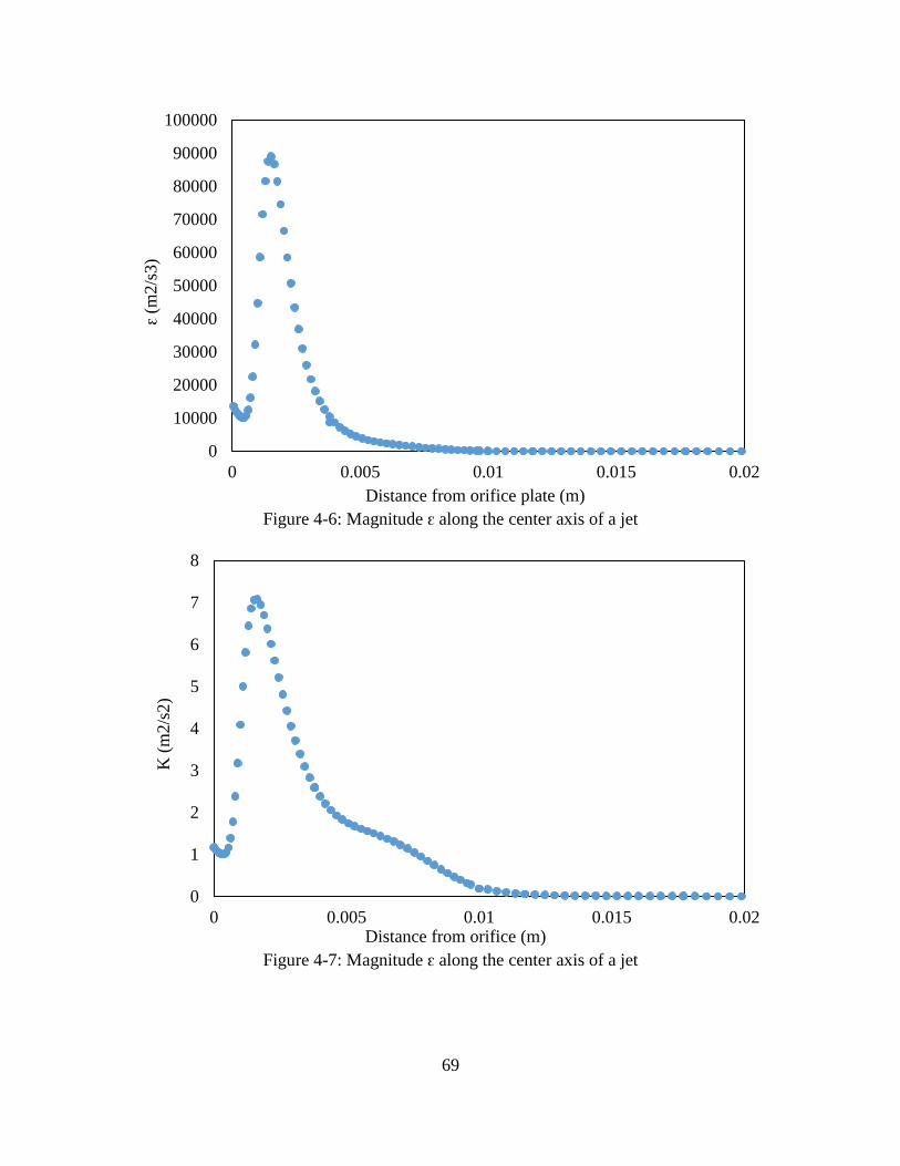
69
Figure 4-6: Magnitude ԑ along the center axis of a jet
Figure 4-7: Magnitude ԑ along the center axis of a jet
0
10000
20000
30000
40000
50000
60000
70000
80000
90000
100000
0 0.005 0.01 0.015 0.02
ԑ(m
2/s
3)
Distance from orifice plate (m)
0
1
2
3
4
5
6
7
8
0 0.005 0.01 0.015 0.02
K (
m2/s
2)
Distance from orifice (m)

70
Full reactor scale modelling, CFD-PBM setup
It is impractical to use the same mesh resolution as in the periodic domain case for simulating
the flow behavior for the full-scale of the reactor. For this reason a coarser mesh with an average
element size of 4mm is used. The Jet region leading towards the orifice plate is progressively
refined as shown in. This type of local mesh refinement allows for reliable representation of the
jets. The liquid jets (orifice plate) were modelled as source points by introducing mass and
momentum source terms in the continuity and momentum equations.
Figure 4-8: Mesh used for the CFD-PBM simulations of the small rig
4.6.1 Source point modelling
The liquid jets (orifice plate) were modelled as source points by introducing mass and
momentum source terms in the continuity and momentum equations. This is performed by marking
the top most layer of cells immediately next to the boundary representing the orifice plate. The
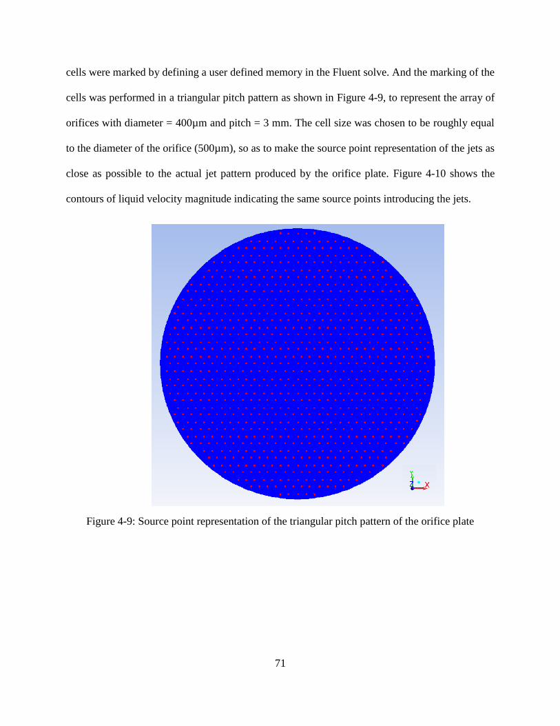
71
cells were marked by defining a user defined memory in the Fluent solve. And the marking of the
cells was performed in a triangular pitch pattern as shown in Figure 4-9, to represent the array of
orifices with diameter = 400µm and pitch = 3 mm. The cell size was chosen to be roughly equal
to the diameter of the orifice (500µm), so as to make the source point representation of the jets as
close as possible to the actual jet pattern produced by the orifice plate. Figure 4-10 shows the
contours of liquid velocity magnitude indicating the same source points introducing the jets.
Figure 4-9: Source point representation of the triangular pitch pattern of the orifice plate

72
Figure 4-10: Contours of Liquid Velocity Magnitude showing the source point representation of
the orifice plate.
The introduction of gas phase at the bottom of the reactor, was also modelled by the use of
introducing source terms in the mass and momentum equations for the Large-bubbles gas phase.
Figure 4-11 shows the resultant holdup contours indicating the gas inlet zones that is representative
of the 3-arm sparger geometry located at the bottom section of the column.

73
Figure 4-11: Contours of Injected large bubble gas Holdup, (a) showing introduction of Gas
(Large Bubbles) from the sparger (b) Source point representation of the three arm gas sparger.
4.6.2 Tuning of CFD-PBM parameters
4.6.2.1 Tuning of 𝑫𝒇,𝒍𝒃 and 𝑫𝒇,𝒔𝒃
The drag force acting on the large bubbles determines the slip velocity of the large bubbles
and hence the rate at which they rise from the bottom to the top (jet region). The slip velocity is a
complex function of bubble diameter, gas volume fraction and interfacial contamination by
surfactants (SDS) and salt (KCl). The Schiller Naumann drag law is applicable for single bubble
rising in infinite medium. For this reason a drag modification factors 𝐷𝑓,𝑙𝑏 and 𝐷𝑓,𝑠𝑏 were
introduced in the drag correlation formulation for the large bubbles phase and micro bubbles phase
respectively.
𝐶𝐷,𝑠𝑏 = 𝐷𝑓,𝑠𝑏 { 24(1 + 0.15 𝑅𝑒𝑠𝑏
0.687)
𝑅𝑒𝑠𝑏 , 𝑅𝑒𝑠𝑏 < 1000
0.44 , 𝑅𝑒𝑠𝑏 ≥ 1000
(4-8)

74
𝐶𝐷,𝑙𝑏 = 𝐷𝑓,𝑙𝑏 {
24(1 + 0.15 𝑅𝑒𝑙𝑏0.687)
𝑅𝑒𝑙𝑏 , 𝑅𝑒𝑙𝑏 < 1000
0.44 , 𝑅𝑒𝑙𝑏 ≥ 1000
(4-9)
To incorporate the effect of above mentioned variables we tuned 𝐷𝑓,𝑙𝑏 and 𝐷𝑓,𝑠𝑏 in equation
(4-8) & (4-9) such that the slip velocity calculated from CFD simulation matches the slip velocity
experienced by the bubbles in the real column. This is achieved by modifying the parameters till
the holdup prediction by the simulations match the holdup measurements from the experiments
(table 2).
4.6.2.2 Tuning of Critical Weber number (Wecrit)
The appropriate value of Wecrit for a given gas liquid system can be obtained by performing
a tuning procedure, by iteratively matching the small bubble diameter and breakage rate from the
CFD results with that of the experimentally observed values. This tuning is performed using the
experimental data for few of the superficial velocities and the tuned value of Wecrit is fixed as a
constant for simulating rest of the combinations of the superficial velocities for the given gas-
liquid system. In our case the air-water gas-liquid system is defined by the kCl and SDS
concentration in the liquid phase. Although Wecrit should purely be a property of the gas-liquid
system, the values of Wecrit obtained by a tuning procedure in a high-resolution simulation of jets
in the periodic box, will almost definitely will not agree with the values obtained from the tuning
procedure based on a full-scale simulation where the jets are modelled as source-points. One
reason for this is that, the average turbulent kinetic energy and the turbulent dissipation rate gets
smeared out in the coarse mesh used for the full-scale simulations. Nevertheless, the full-scale
simulations allow us to study the global circulations, 3-phase hydrodynamics and RTD response

75
of the reactor. This also highlights, the need for performing the tuning procedure for Wecrit every
time when the mesh resolution near the jet region changes.
Figure 4-12: Tuning of Wecrit for small rig with sparger at bottom, VG = 10mm/s and VL = 78
mm/s introduction of Gas (Large Bubbles phase) from the sparger.
Results
By following the above mentioned tuning procedure and using the experimental data
obtained from the small rig with sparger at bottom, for the gas liquid system of SDS =25ppm and
KCl=75ppm, the optimum values for the parameters 𝐷𝑓,𝑙𝑏 , 𝐷𝑓,𝑠𝑏 and Wecrit were obtained for the
superficial velocities of VG = 2mm/s and VL = 78 mm/s; and VG=2mm/s and VL =93 mm/s. After
extensive tuning the following values were used for the parameters: 𝐷𝑓,𝑙𝑏 =1.5, 𝐷𝑓,𝑠𝑏 =0.5 and
0.00
50.00
100.00
150.00
200.00
250.00
300.00
350.00
0.00 1.00 2.00 3.00 4.00 5.00 6.00
Bu
bb
le s
ize
D32 (m
icro
ns)
Wecrit
jets (as source points)
jets (resolved)
Exp_dia

76
Wecrit = 0.5. Some of the qualitative and quantitative results obtained from the simulations
performed using these tuned parameter values are presented in this section.
Figure 4-13(a) and Figure 4-14 show the contours of large bubbles volume fraction on the center
plane and cut planes respectively. It can be seen that the large bubble plume is preserved inspite
of turbulent dispersion (dk = 0.5). It can also be seen that the bubbles have accumulated at the top
forming a froth layer. Figure 4-13(b) and Figure 4-15 show the contours of small bubbles volume
fraction over the center plane and cut planes respectively. It could be seen that the holdup of small
bubbles is more uniform, especially in the fully developed central region of the column. This could
be attributed to the low slip velocity of the micro bubbles.
Figure 4-13: Contours of gas holdup of for VG = 2mm/s and VL = 78 mm/s: (a) Injected large
bubbles (b) Micro-bubbles
(a) (b)

77
Figure 4-14: Contours of Large bubbles holdup for VG = 2mm/s and VL = 78 mm/s
Figure 4-15: Contours of micro bubbles holdup for VG = 2mm/s and VL = 78 mm/s
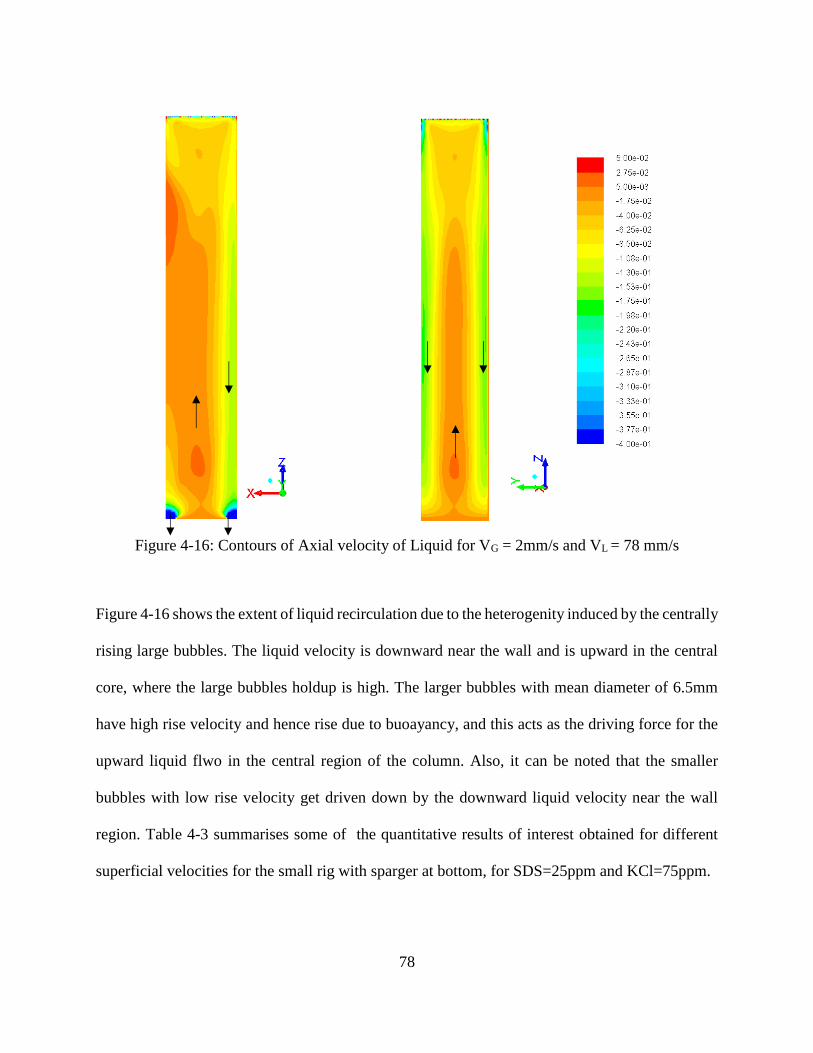
78
Figure 4-16: Contours of Axial velocity of Liquid for VG = 2mm/s and VL = 78 mm/s
Figure 4-16 shows the extent of liquid recirculation due to the heterogenity induced by the centrally
rising large bubbles. The liquid velocity is downward near the wall and is upward in the central
core, where the large bubbles holdup is high. The larger bubbles with mean diameter of 6.5mm
have high rise velocity and hence rise due to buoayancy, and this acts as the driving force for the
upward liquid flwo in the central region of the column. Also, it can be noted that the smaller
bubbles with low rise velocity get driven down by the downward liquid velocity near the wall
region. Table 4-3 summarises some of the quantitative results of interest obtained for different
superficial velocities for the small rig with sparger at bottom, for SDS=25ppm and KCl=75ppm.

79
Table 4-3: CFD-PBM results for different superficial velocities for the small rig geometry with
the sparger at bottom; for SDS =25ppm and KCl=75ppm.
VG VL gas holdup
Bubble
Diameter Interfacial area
Exp CFD Exp CFD Exp CFD
mm/s mm/s % % µm µm m2/m3 m2/m3
2.06 78 6.3 6.0 253 278 1490 999
2.06 93 2.0 4.9 162 274 741 770
6.17 78 14.6 10.0 211 284 4162 1503
6.17 93 13.7 7.8 192 260 4276 1008
10.3 78 25.6 8.9 201 276 7647 890
10.3 93 20.4 9.6 179 246 6827 872
Mass transfer modelling
The mass transfer rate in the experiments were measured in terms of Kl*ai (hr-1) values
obtained by measuring the difference in the oxygen concentration in the liquid phase at the inlet
and at the outlet of the reactor using dissolved oxygen sensors. In the CFD-PBM simulations, the
Kl*ai values were calculated from the converged results (flow field values). The interfacial area ai
(m2/m3) was estimated based on the Sauter mean diameter D32 for the large bubble and small
bubble phase in each cell, using equation Eq.(4-11). Similarly the mass transfer coefficient Kl was
estimated in each cell using the Ranz-Marshal correlation (Ranz, 1952) as given by equation
Eq.(4-11).
Kl from Ranz-Marshal correlation is defined as:
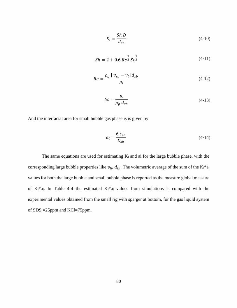
80
𝐾𝑙 =
𝑆ℎ 𝐷
𝑑𝑠𝑏 (4-10)
𝑆ℎ = 2 + 0.6 𝑅𝑒
12 𝑆𝑐
13 (4-11)
𝑅𝑒 =
𝜌𝑔 | 𝑣𝑠𝑏 − 𝑣𝑙 |𝑑𝑠𝑏
𝜇𝑙 (4-12)
𝑆𝑐 =𝜇𝑙
𝜌𝑔 𝑑𝑠𝑏 (4-13)
And the interfacial area for small bubble gas phase is is given by:
𝑎𝑖 =
6 𝜖𝑠𝑏𝐷𝑠𝑏
(4-14)
The same equations are used for estimating Kl and ai for the large bubble phase, with the
corresponding large bubble properties like 𝑣𝑙𝑏 𝑑𝑙𝑏. The volumetric average of the sum of the Kl*ai
values for both the large bubble and small bubble phase is reported as the measure global measure
of Kl*ai. In Table 4-4 the estimated Kl*ai values from simulations is compared with the
experimental values obtained from the small rig with sparger at bottom, for the gas liquid system
of SDS =25ppm and KCl=75ppm.
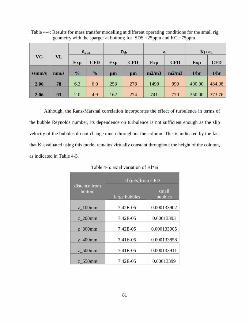
81
Table 4-4: Results for mass transfer modelling at different operating conditions for the small rig
geometry with the sparger at bottom; for SDS =25ppm and KCl=75ppm.
VG VL
𝝐𝒈𝒂𝒔 Dsb ai Kl * ai
Exp CFD Exp CFD Exp CFD Exp CFD
ssmm/s mm/s % % µm µm m2/m3 m2/m3 1/hr 1/hr
2.06 78 6.3 6.0 253 278 1490 999 400.00 484.08
2.06 93 2.0 4.9 162 274 741 770 350.00 373.76
Although, the Ranz-Marshal correlation incorporates the effect of turbulence in terms of
the bubble Reynolds number, its dependence on turbulence is not sufficient enough as the slip
velocity of the bubbles do not change much throughout the column. This is indicated by the fact
that Kl evaluated using this model remains virtually constant throughout the height of the column,
as indicated in Table 4-5.
Table 4-5: axial variation of Kl*ai
distance from
bottom
kl (m/s)from CFD
large bubbles
small
bubbles
z_100mm 7.42E-05 0.000133902
z_200mm 7.42E-05 0.00013393
z_300mm 7.42E-05 0.000133905
z_400mm 7.41E-05 0.000133858
z_500mm 7.41E-05 0.000133911
z_550mm 7.42E-05 0.00013399

82
This highlights the need for a mass transfer model that can take in to account the effect of local
turbulence from the 𝑘-𝜀 model. One such correlation was proposed by Calderbank & Moo-Young
in 1961(Calderbank and Moo-Young, 1961), for estimating the liquid side mass transfer
coefficient in aerated mixing vessels, where high values of 𝜀 is common place.
𝐾𝑙 = 0.13 𝑆𝑐−23 (
𝜀 𝜇𝑙
𝜌𝑙2 )
14
(4-15)
In order to take account for this fact, we plan to use a linear combination of Ranz-Marshal
type and Calderbank type models in the future for estimation of Kl. By using a linear combination
of these two models we expect that the Calderbank model will be dominant at regions of high
turbulent dissipation rate 𝜀, and the Ranz-Marshal model will be dominant in regions were 𝜀 is
low.
RTD studies from CFD-PBM model
In experiments the Residence Time Distribution (RTD) data was obtained by introducing a
pulse input of a salt tracer, and monitoring it’s concentration at various locations of the reactor
using conductivity probes. For determining the RTD from the 3D CFD-PBM model, a species
transport equation was solved in addition to the existing Euler-Euler and PBM equations. The new
specie introduce by the tracer was considered to be a neutrally buoyant fluid with the same
properties as the continuous phase (liquid: water). The diffusion coefficient in the species transport
equation was set to be equal to the self-diffusion coefficient for water at 25oC (Dtracer=2.29e-9
m2/s). The required Mass fraction of the tracer was patched as a function of time to match the
injection pulse of the tracer in the actual RTD experiments. In this case the injection pulse was
obtained from the normalized RTD curve in the Head section (flushed against wall) from the

83
experimental RTD data obtained from the small rig with sparger at the bottom, and for the
superficial velocities of VG=4.11 and VL=77.8 mm/s. Subsequently the RTD curves were obtained
by monitoring mass fraction of the neutrally buoyant tracer at the corresponding locations (Top,
middle and bottom) as in the Experimental setup.
Table 4-6 shows the exact location of the monitor points used in the CFD case that
corresponds to the location of the salt-tracer-sensors in the experimental setup.
Table 4-6: Location of tracer fraction monitors corresponding to the conductivity probe locations
in RTD salt tracer experiments.
Monitor
location
x y z
m m m
Top 0.0248 0.0429 0.4900
Middle 0.0248 0.0429 0.3100
Bottom 0.0248 0.0429 0.1400
The RTD results from CFD and Experiments are shown in Figure 4-17 and Figure 4-18. In
the experimental RTD curves, a few features are worth highlighting. The peak in the mid-sensor
is observed almost at the same instant as the top sensor. This indicates presence of large circulating
eddy short circuiting the section between these two sensors. Such behavior is indicative of a purely
back-mixed reactor. This could be attributed to the circulation cell generated by the rising larger
bubbles.

84
Figure 4-17: RTD from CFD for Small Rig, for VG = 4.11 mm/s and VL = 77.82 mm/s, 3 arm
sparger at bottom
0
0.1
0.2
0.3
0.4
0.5
0.6
0.7
0.8
0.9
1
2 4 6 8 10 12 14 16 18 20
Mas
s fr
acti
on o
f tr
acer
(-)
Time (s)
Injection pulse
Top
Middle
Bottom
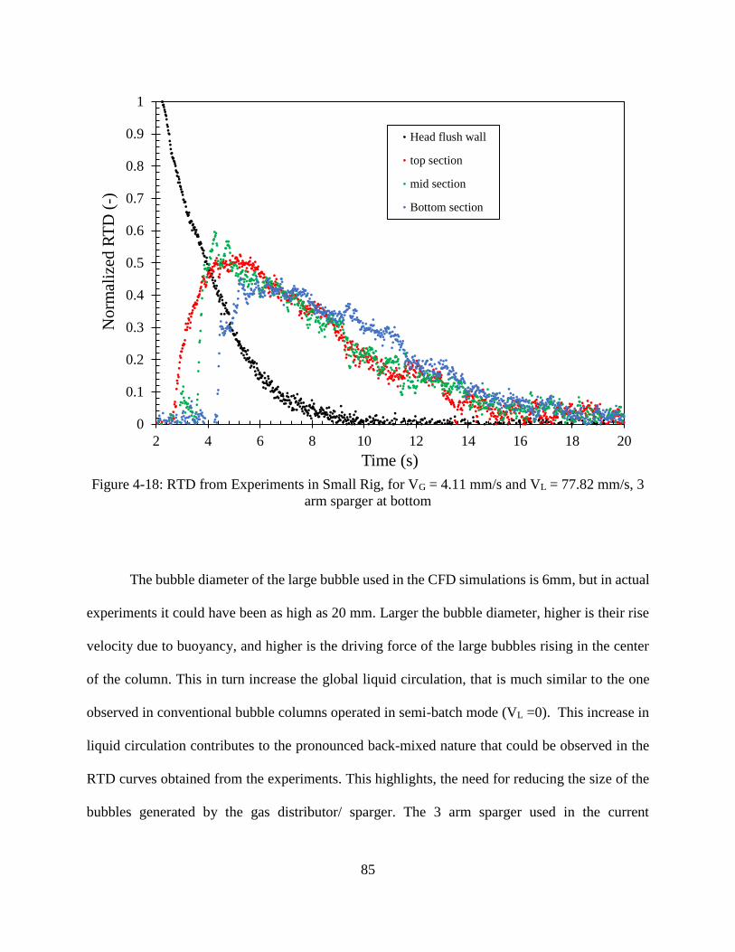
85
Figure 4-18: RTD from Experiments in Small Rig, for VG = 4.11 mm/s and VL = 77.82 mm/s, 3
arm sparger at bottom
The bubble diameter of the large bubble used in the CFD simulations is 6mm, but in actual
experiments it could have been as high as 20 mm. Larger the bubble diameter, higher is their rise
velocity due to buoyancy, and higher is the driving force of the large bubbles rising in the center
of the column. This in turn increase the global liquid circulation, that is much similar to the one
observed in conventional bubble columns operated in semi-batch mode (VL =0). This increase in
liquid circulation contributes to the pronounced back-mixed nature that could be observed in the
RTD curves obtained from the experiments. This highlights, the need for reducing the size of the
bubbles generated by the gas distributor/ sparger. The 3 arm sparger used in the current
0
0.1
0.2
0.3
0.4
0.5
0.6
0.7
0.8
0.9
1
2 4 6 8 10 12 14 16 18 20
No
rmal
ized
RT
D (
-)
Time (s)
Head flush wall
top section
mid section
Bottom section
86
experiments consists of 12 holes and this leads to formation of large bubbles (~20 mm), by
replacing each of the arms with a sintered sparger will lead to a more uniform injection of bubbles
and will also lead to formation of bubble of considerably small diameter (~1 to 5 mm) and this
will bring down their rise velocity and also will in turn reduce the extent of the liquid circulation
associated with it.
Conclusions
We have demonstrated the use of CFD-PBM coupled models to capture the complex
multiphase-flow behavior encountered in the novel down-flow bubble column of diameter 10 cm.
The use of PBM model with the breakage kernel, allowed for capturing the breakage of injected
large bubbles to micro-bubbles. The velocity fields of the large bubble and micro-bubbles were
captured by separately using the in-homogeneous discrete model of the PBM. The modelling of
the orifice plate and the gas sparger was performed using source point modelling. The CFD-PBM
model was also used to model the jet region in a periodic domain. Further the extension of the
CFD-PBM model setup was used to perform RTD studies and also Mass transfer modelling.
Although the CFD-PBM model was successful in modelling the breakage process i.e. in predicting
the micro-bubble diameter, the proper choice of the breakage kernel and tuning of the parameters
in the breakage kernel Wecrit proved to be difficult, and for this reason the CFD-PBM modelling
has been abandoned in the following chapter. In the next chapter, we discuss the modelling of a
novel down-flow bubble column of much larger cross-section of 30 cm diameter, using a pure
Euler-Euler description and capturing the breakage or conversion of the injected large bubbles to
micro-bubbles by using appropriate source and sink terms in jet region immediately below the
orifice plate.

87
Chapter 5. CFD Study of the Extent and Nature of Liquid Circulations in a
Novel Down-Flow Bubble Column of 30 cm Column Diameter
Introduction
In the presented work, we demonstrate the successful use of the novel gas-liquid injection
mechanism in a column of much larger cross-section (0.3 mm diameter). The experiments and
CFD analysis have been carried out to bring out the flow characteristics, particularly, the extent of
liquid phase re-circulation in this column of large cross-section. As the experimental methods that
have been used in this work are already well established, the real challenge lies in the CFD
simulation of this complex system with the presence of fine liquid jets and the gas phase with two
distinct classes of bubble sizes i.e. the injected large bubbles (of about 7 mm) and the micro-
bubbles (300-800µm) produced form the jet zone. The CFD simulations have been setup neither
with an objective of capturing the finer/resolved details of the array of liquid jets, nor with an
objective to exact the process of breakage of the injected larger bubbles to finer micro-bubbles by
these jets. In fact, the accurate numerical modelling of these phenomena is computationally
expensive and also such simulations do not provide any real value from the perspective of scale-
up analysis or largescale reactor design and sizing. Instead, the setup of the CFD simulations is
geared more towards capturing the impact of these phenomena on the large-scale liquid circulation
and flow patterns observed at the reactor scale. Additionally, due to the disparity in the formulation
of the drag laws available for the simulation of bubbly flows in the Euler-Euler framework, a drag
modification factor (section 2.3.1) is used to improve the accuracy of the CFD simulations. The
drag modification factor has been formulated in such a way to take into account, the swarm effect
(local gas holdup dependence) and also the effect of the surface-active additives on the gas-liquid
interface. This drag modification factor is calculated for each one of the drag laws previously

88
reported in the literature, from a simple force balance based on experimentally obtained global
(volume average) gas hold-up values measured for different operating conditions. This is achieved
by using an optimization routine, to obtain the optimum values of the parameters used in the drag-
modification factor, for the different drag-correlations that are available in the literature Further,
the radial gas hold-up measurements from the Gamma Ray Densitometry (GRD) is used to validate
the CFD results. Finally, the radial profiles of axial liquid velocities obtained from the validated
CFD model provides better insights into the flow behavior of the considered Down-flow bubble
column at different operating conditions.
Experimental setup:
The experiments were performed in a 0.3 m diameter and 1.5 m long clear Perspex column
using an air-water system with 20 PPM surfactant (SDS). The addition of the surfactant was to
suppress the coalescence of bubbles (Kleinbart et al., 2016). The liquid enters the column from the
top through the orifice plate with 1mm diameter holes arranged in triangular pitch. The gas is
sparged at a location 100 mm below the orifice plate using an eight arm sparger, each arm separated
by 450 angle and with 5 holes per arm with a hole-diameter of 1.2mm. The incoming liquid forms
intense liquid jets which help in breaking up the sparged bubbles (about 7 mm) rising from the gas
sparger into micron-size bubbles. As the micro-bubbles exhibit less rise velocity, these generated
micro-bubbles flow along with the liquid flowing downwards.

89
Figure 5-1: Schematic of the Down-flow bubble column
The present experimental set-up as shown in Figure 1A and 1B, offers flow regimes and
flow patterns that are different from conventional down-flow bubble columns reported in the
literature. The co-current downward flow operation can be achieved only for a limited number of
liquid and gas flow rates, as the gas phase and liquid phase flow rates need to satisfy the mass
balance which permits stable steady state operation of the column. Basically, the downward true
velocity of liquid (VL/𝜖𝐿) needs to be higher than the terminal rise velocity of bubbles. The

90
operating window at which stable down-flow conditions could be achieved were found to be in
the range of superficial liquid velocity (VL = 58-75 mm/s) and superficial gas velocity (VG = 2.5-
18 mm/s).
5.2.1 Volumetric gas hold-up measurement
For the volumetric gas hold-up measurement, Phase-isolation technique was used. In this
method, after achieving the stable operating condition, the inflow and outflow of the liquid and
gas flow to the column is shut off. Enough time is provided for the complete disengagement of the
gas bubbles from the liquid phase and then the clear gas-liquid heights are measured and used to
determine the volume averaged gas hold-up (Kalaga et al., 2016; Kalaga, 2015) .
𝜖�̅� =
𝐻𝑒𝑖𝑔ℎ𝑡 𝑜𝑓𝑔𝑎𝑠 𝑝ℎ𝑎𝑠𝑒
𝑇𝑜𝑡𝑎𝑙 ℎ𝑒𝑖𝑔ℎ𝑡 𝑜𝑓𝑡𝑤𝑜 𝑝ℎ𝑎𝑠𝑒 𝑚𝑖𝑥𝑡𝑢𝑟𝑒 (1)
5.2.2 Measurement of axial variation of gas hold-up
The second technique, is based on the pressure drop, which uses the measurement of axial
pressure variation. The pressure inside the column was measured using highly responsive and
accurate pressure transducers (Omega Engineering, USA) flush mounted to the column wall (Fig.
1B) at different axial locations of 0.085, 0.215, 0.505, 0.64 and 1.035 m from the orifice plate. The
volume averaged void fraction between two pressure transducers P1 and P2, is calculated using the
pressure difference method by using the equation below (Kalaga et al., 2016).
𝜖�̅�,12 =
(𝑃2 − 𝑃1)𝑇𝑃 − (𝑃2 − 𝑃1)𝐿(𝑃2 − 𝑃1)𝐿 − (𝑃2 − 𝑃1)𝐺
(2)
Where,
(𝑃2 − 𝑃1)𝐺 - pressure drop recorded for only air.

91
(𝑃2 − 𝑃1)𝐿 -pressure drop recorded for only liquid.
(𝑃2 − 𝑃1)𝑇𝑃 - pressure drop recorded for two-phase, gas-liquid dispersion.
5.2.3 Measurement of radial variation of gas hold-up
In addition to the above two hold-up measurements, GRD technique was used for the chordal
hold-up measurements at different radial locations. GRD is a non-invasive technique and consists
of a gamma source (5 mCi Cs-137) and a 2”×2” NaI scintillation detector. Bothe the source and
the detector were installed directly opposite to each other on a U-shaped metal platform free to
traverse along the radius of the column as shown in Figure 2.
Figure 5-2: Experimental setup for the Gamma Ray Densitometry.
The gamma measurements were made at a plane 1 m below the orifice plate and for five
different chordal locations. Each measurement scan was made for a duration of five minutes. The
gamma beam intensity transmitted through a material of length X was calculated using the Beer-
NaI detector

92
Lambert’s law given by the following equation (Chavan et al., 2009; Hernandez-Alvarado et al.,
2017b; Kalaga et al., 2009):
𝐼 = 𝐼0𝑒−𝛽𝑋 (3)
Where I0 is the incident gamma beam intensity, I is the transmitted beam intensity, and 𝛽 is the
linear attenuation coefficient, which depends on the material between the gamma source and
detector. The intensity of gamma-ray beam passing through a heterogeneous medium consisting
of materials in series with different attenuation coefficients,𝛽𝑖, and thicknesses, Xi, can be given
by following equation
𝐼 = 𝐼0𝑒−∑𝛽𝑖𝑋𝑖 (4)
The linear attenuation coefficients were determined by making the measurements in the column
filled with gas, and then with liquid. The void fraction under the operating condition was then
estimated by using the following equation (Hernandez-Alvarado et al., 2017b) :
𝜖𝐺 =𝑙𝑛 (
𝐼𝑇𝑃𝐼𝐿)
𝑙𝑛 (𝐼𝐺𝐼𝐿)
(5)
Where IG and IL are the gamma intensities detected when the column is filled with gas and liquid,
respectively, and ITP is the intensity detected when the column is in actual operation, filled with a
two-phase mixture of liquid and gas bubbles.
93
5.2.4 Measurement of bubble size distribution
In addition to the three hold-up measurement techniques, the bubble size measurements
were performed using a photographic technique. A high-speed video camera (Photron-UX100)
connected to a borescope (Hawkeye Pro) and equipped with a DC source bright LED light
(Luxxor-50) was used for recording images of the micro-bubbles in the gas liquid dispersion. The
measurements were performed at two axial locations of 0.5 and 1.0 m below the orifice plate. At
each axial location, radial variation of the bubble size was measured by pacing the borescope from
the center of the column towards the wall, and the images were recorder at three different radial
locations (r/R = 0, 0.5, 1). The maximum bubble diameter that can be seen using the borescope is
15 mm. The frame rate and the shutter speed of the high-speed camera were adjusted according to
the gas and liquid flowrates. The digital photographs were processed and enhanced by using Image
Processing Software (PFV Ver.350) that enabled to distinguish clearly the bubble boundaries. A
prior calibration of the pixel to pixel distance was made and the actual bubble sizes were measured
manually using the PFV software. Figure 3 shows an image of the micro-bubbles inside the
column, as captured using the boroscope and high speed camera assembly. Unlike the bubble
shapes encountered in conventional bubble columns, the micro-bubbles generated in the current
system are strongly spherical in shape. The images were recorded at different frame rates ranging
from 1000 to 6000 FPS depending on the two-phase flow velocity. In order to get the bubble size
distribution and the mean bubble size, approximately 800 to 1000 focused bubbles were measured
from 3000–4000 recorded images.

94
Figure 5-3: Image of the two-phase bubbly flow as captured by the high-speed camera using the
boroscope
Drag modification factor from force balance method
In order to address this huge variation in the available drag correlations and also the associated
drag modification factors, we propose a simple force balance method based on the experimental
global measurements of the gas hold-up. To that end, in the present work, a drag modification
factor ′𝐷𝑓′ is used to take into account the effect of both the presence of surface-active agents and
the local gas hold-up on the drag force experienced by the bubble swarm.
𝐷𝑓 = (1 + 𝛼) ∗ (1 − 𝜖𝐺)𝑛 (6)
Here, the parameter ‘𝛼′ takes into account the effect of the presence of additives like surface-
active agents on the gas-liquid interface, and the exponent ‘n’ determines the effect of the local
gas-holdup. Further, the optimum values of the above parameters ‘𝛼′ and ‘n’ for each one of the
available drag-correlations, are obtained from a simple force balance involving only the buoyancy

95
force and the drag force acting on the bubbles. Such a force balance is performed for a control
volume of unit size with an uniform gas hold-up of 𝜖𝐺. By comparing the slip velocities obtained
from such a force balance (Eq.21) with that of the experimentally observed average slip velocities
(Eq.22) for the nine different operating conditions, the optimum values of ‘𝛼′ and ‘n’ are obtained
for each one of the drag correlations. Figure 4 shows the slip velocity predictions from the force
balance model for the different drag correlations without any modification (𝐷𝑓 =1).
𝐹𝑑𝑟𝑎𝑔 = 𝐷𝑓
𝐴𝑖8𝐶𝐷𝜌𝑙|𝑣𝐿 − 𝑣𝐺| (𝑣𝐿 − 𝑣𝐺) , 𝐴𝑖 =
6𝜖𝐺(1 − 𝜖𝐺)
𝑑𝐵 (7)
𝐹𝐵 = 𝜖𝐺 𝑔 (𝜌𝐿 − 𝜌𝐺) (8)
Equating the modified drag force to the buoyancy force we obtain:
𝑉𝑠𝑓𝑏 = √4𝑑𝐵3𝐷𝑓𝐶𝐷
𝜖𝐺(𝜖𝐿 − 𝜖𝐺)
(𝜌𝐿 − 𝜌𝐺𝜌𝐿
) 𝑔 (9)
𝑉𝑠𝑓𝑏 = √4𝑑𝐵
3(1 + 𝛼)(1 − 𝜖𝐺)𝑛 𝐶𝐷
𝜖𝐺(𝜖𝐿 − 𝜖𝐺)
(𝜌𝐿 − 𝜌𝐺𝜌𝐿
) 𝑔 (10)
The slip velocity computed from Experimental global hold-up measurements is calculated as:
𝑉𝑠𝑒𝑥𝑝 =
𝑉𝐿𝜖𝐿−𝑉𝐺𝜖𝐺
(11)

96
Figure 5-4: Comparison between average slip velocity from experiments (𝑉𝑠𝑒𝑥𝑝) and slip
velocity predicted from force balance (𝑉𝑠𝑓𝑏) for 𝐷𝑓 =1: ○ Schiller Naumann, + Dalla Ville, □
Clift, ♦ Ma&Ahmadi, ■ Mei et al , ● Lain et al, ◊ Tomiyama 1998, - Tomiyama 2002, ▲ Zhang
& VanderHeyden.
Figure 5 shows the slip velocity predictions from the force balance, after using the
optimized values of ‘𝛼′ and ‘n’ for each one of the drag correlation considered. The optimum
values of ‘𝛼′ and ‘n’ for the different drag correlations (𝐶𝐷 formulations listed in Table 2) where
obtained by minimizing the cumulative error ∑(𝑉𝑠𝑓𝑏 − 𝑉𝑠𝑒𝑥𝑝)2
, using the MATLAB® function
“fmincon”. The lower and upper bounds for ′𝛼′ and ‘n’ were set to (-0.5, 2) and (-3, 3) respectively.
40
60
80
100
120
140
160
40 50 60 70 80 90 100 110
Ave
rage
slip
vel
oci
ty f
rom
fo
rce
bal
ance
, 𝑉𝑠
fb (
mm
/s)
Experimental average slip velocity 𝑉𝑠 𝑒𝑥𝑝 (mm/s)
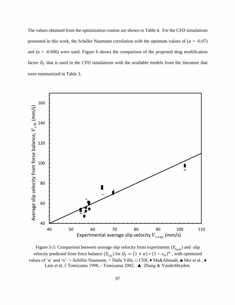
97
The values obtained from the optimization routine are shown in Table 4. For the CFD simulations
presented in this work, the Schiller Naumann correlation with the optimum values of (𝛼 = -0.07)
and (n = -0.696) were used. Figure 6 shows the comparison of the proposed drag modification
factor 𝐷𝑓 that is used in the CFD simulations with the available models from the literature that
were summarized in Table 3.
Figure 5-5: Comparison between average slip velocity from experiments (𝑉𝑠𝑒𝑥𝑝) and slip
velocity predicted from force balance (𝑉𝑠𝑓𝑏) for 𝐷𝑓 = (1 + 𝛼) ∗ (1 − 𝜖𝐺)𝑛 , with optimized
values of ‘α’ and ‘n’: ○ Schiller Naumann, + Dalla Ville, □ Clift, ♦ Ma&Ahmadi, ■ Mei et al , ●
Lain et al, ◊ Tomiyama 1998, - Tomiyama 2002, ▲ Zhang & VanderHeyden.
40
60
80
100
120
140
160
40 50 60 70 80 90 100 110
Ave
rage
slip
vel
oci
ty f
rom
fo
rce
bal
ance
, 𝑉𝑠
fb (
mm
/s)
Experimental average slip velocity 𝑉𝑠 𝑒𝑥𝑝 (mm/s)

98
Table 5-1: Optimized values of ‘α’ and ‘n’ in 𝐷𝑓 = (1 + 𝛼) ∗ (1 − 𝜖𝐺)𝑛 for the different drag
correlations obtained from the force balance method.
Drag model 𝜶 𝒏
Schiller and Naumann (1935) -0.07 -0.70
Dalla Ville (1948) -0.16 -0.69
Clift et al. (2005) -0.07 -0.70
Ma and Ahmadi (1990) 0.05 -0.68
Mei et al. (1994) 0.64 -1.14
Laı́n et al. (2002) 0.64 -1.06
Tomiyama et al. (1998) -0.03 -0.63
Tomiyama (2004) 0.88 0.77
Zhang and VanderHeyden (2002) -0.11 -0.63

99
Figure 5-6: Comparison between various formulations of the drag modification factor 𝐷𝑓
CFD simulation setup
The 3D Finite Volume Method (FVM) based Euler-Euler simulations were carried out using
the FLUENT software (ANSYS 15.0, Inc.). Due to the unique design of the column under
consideration, wherein the micro-bubbles are generated in the jet region by breakage of the large
bubbles injected from the gas sparger, two distinct classes of bubbles with very different mean
bubble sizes are present in the system. Due to the difference in the mean bubble size of these two

100
classes of bubbles, they also experience different slip velocities, for this reason these two different
bubble classes are treated as two different gas-phases for modelling purposes. Further, the
conversion of the injected large-bubbles to micro-bubbles takes place only in a region right below
the orifice plate where the array of fine jets is created. The kinetic energy and turbulence generated
by the injected liquid jets aids in the breakage of the injected large bubbles. This is a complex
process and the coarse grid used for the current Euler-Euler model is insufficient to accurately
capture this process even when coupled with a Population Balance Model (PBM). Further once
the micro-bubbles leave the highly turbulent jet region, their bubble size distribution remains stable
as the micro-bubble dispersion gets dragged downstream by the liquid flow. For this reason, a
mass conversion User Defined Function (UDF) is used in the cells in the jet region immediately
below the orifice plate. The mass conversion UDF involves the use of a sink term in the large-
bubble phase continuity equation and an equivalent source term in the micro-bubble phase
continuity equation. For the microbubble phase average of the experimentally observed mean
bubble size from the high-speed camera measurements, was used as the input to the CFD
simulations. For the injected large bubble phase, a constant bubble diameter of 7 mm was used.

101
Figure 5-7: Mesh used for the CFD simulations
Figure 7 shows the mesh used for the simulations with a size of 2M cells. The top orifice-plate
and the cylindrical surface were modelled as a wall-boundary with zero slip and the outlet at the
bottom of the column was modelled as a pressure outlet. Fluent UDFs were used for source-point
modelling of the gas and liquid injection points. Source point modeling involves the introduction
of mass and momentum source terms in the continuity and momentum equations respectively in
the cells where the injection points are located. This allows for the use of a coarse grid without the
need to refine the finer details of the injection points of the orifice plate or the gas sparger. Figure
5-8 shows the source point representation of the 8-arm gas sparger. Each arm of the sparger was
of 5 inch length and 0.4 inch diameter, which contributes to a blocked area of less than 0.4% of
the column cross-sectional area. For this reason, the wall effects resulting from the sparger piping
is considered insignificant when compared to the column scale dynamics and is not modelled in

102
the simulations. Similarly, the injection of the liquid jets through the orifice plate is also modelled
as source points. Figure 5-9 shows the source point representation of the holes arranged in
triangular pitch in the orifice plates.
Figure 5-8: Source point representation of the 8-arm gas sparger, the cells marked for gas
injection are shown in red

103
Figure 5-9: Source point representation of the orifice plate, the cells marked for Liquid injection
are shown in white.
Results and discussion
5.5.1 Volumetric and axial variation of gas hold-up
The measurements were performed for a combination of three different gas (VG = 2.5, 10.2
and 17.8 mm/s) and liquid (VL = 62.24, 70.17 and 78.83 mm/s) superficial velocities. Figure 10
shows the variation of volumetric gas hold-up obtained from the phase-isolation technique for the
9 different operating conditions.

104
Figure 5-10: Volumetric gas hold-up measured using the phase isolation technique. ● VL =
62.24 mm/s, ▲ VL = 70.17 mm/s, + VL = 78.83 mm/s.
It could also be observed that within the operating window, the gas hold-up increases with an
increase in VG and decreases with an increase in VL, as observed in conventional down-flow bubble
columns (Table1). The maximum gas hold-up of 0.54 was observed for the combination of
maximum superficial gas velocity (VG = 17.8 mm/s) and minimum superficial liquid velocity (VL
= 62.24 mm/s). The gas hold-up calculated from different pairs of the pressure transducers, give
the gas hold-up in the corresponding axial sections determined by the locations of the pressure
sensors as depicted in Figure 1B. Figures 11-13 show the axial variation of gas hold-up as
measured form the pressure transducers. It could be observed that unlike in conventional down-
flow bubble columns employing a plunging jet, where the axial variation of gas hold-up is
significant, here the hold-up value remains practically constant in the axial direction. Further
0.00
0.10
0.20
0.30
0.40
0.50
0.60
0 5 10 15 20
Frac
tio
nal
gas
ho
ld-u
p, ϵ
G(-
)
Superficial gas velocity, VG (mm/s)

105
sensors P1 and P5 were the farthest apart and hence the corresponding hold-up measurement form
these two points is closer to the values obtained from the phase-isolation technique (volume
averaged).
Figure 5-11: Axial variation of volumetric gas hold-up from Pressure Transducers for VL =
62.24mm/s
0
0.1
0.2
0.3
0.4
0.5
0.6
0.7
(P1-P2) (P2-P3) (P3-P4) (P4-P5) (P1-P5)
Frac
tio
nal
gas
ho
ld-u
p, ϵ
G(-
)
Pressure Transducers
VG = 2.5 mm/s VG = 10.2 mm/s VG = 17.8 mm/s

106
Figure 5-12: Axial variation of volumetric gas hold-up from Pressure Transducers for VL =
70.17mm/s
Figure 5-13: Axial variation of volumetric gas hold-up from Pressure Transducers for VL =
78.83mm/s
0
0.05
0.1
0.15
0.2
0.25
0.3
0.35
0.4
0.45
(P1-P2) (P2-P3) (P3-P4) (P4-P5) (P1-P5)
Frac
tio
nal
gas
ho
ld-u
p, ϵ
G(-
)
Pressure Transducers
VG = 2.5 mm/s VG = 10.2 mm/s VG = 17.8 mm/s
0
0.05
0.1
0.15
0.2
0.25
0.3
0.35
0.4
(P1-P2) (P2-P3) (P3-P4) (P4-P5) (P1-P5)
Frac
tio
nal
gas
ho
ld-u
p, ϵ
G(-
)
Pressure Transducers
VG = 2.5 mm/s VG = 10.2 mm/s VG = 17.8 mm/s

107
From the volumetric gas hold-up data obtained from the phase-isolation technique drift-flux
analysis was performed using the method of Wallis (Wallis, 1969) and the drift-flux plot is shown
in Figure 14. Here the drift-flux VGL is defined as VGL = 𝜖𝐺VL - 𝜖𝐿VG. As there is no sharp change
in the slope of the 𝜖𝐺 vs VG plot (Figure 10) and the drift-flux plot of VGL vs 𝜖𝐺 (Figure 14), this
indicates that the down-flow column under consideration seems to operate in the homogenous
regime even up to a maximum gas hold-up of 0.54. This is much higher than the typical values of
critical gas hold-up (at which regime transition takes place from homogeneous to heterogeneous
flow conditions) for conventional up-flow bubble columns which is usually in the range of 0.1 to
0.2 (Hernandez-Alvarado et al., 2016; Joshi, 2001; Thorat and Joshi, 2004). However, since the
drift flux analysis is based on a single value of global measurement of volumetric gas hold-up, to
get a better picture of the operating regime (homogeneous or heterogeneous flow), it is important
to undertake actual measurement of the radial profile of the local gas hold-up or the interstitial
liquid velocity.

108
Figure 5-14: Drift flux plot
5.5.2 Radial variation of bubble size distribution
The bubble size measurements were performed at a plane 1m below the orifice-plate using the
boroscope and high-speed camera setup at three different radial locations (r/R= 0,0.5 and 1).
Figures 15-17 show the bubble size distributions obtained for the nine different operating
conditions at these three different radial locations. Figures 18-20, show the radial variation of the
mean bubble size calculated from the bubble size distributions. It can be observed that for a given
operating condition there is also no significant radial variation of the mean bubble size. Further it
can be observed that the mean bubble size decreases with increase in liquid superficial velocity
(VL), this shows that increase in liquid injection rate increases the velocity of the jets, and more
intense jets provide more energy for the breakage of the injected bubbles to much finer micro-
bubbles. Similarly, it can be observed that the mean bubble size increase with increase in gas
0
5
10
15
20
25
30
0 0.1 0.2 0.3 0.4 0.5 0.6
Dri
ft f
lux,
VG
L (m
/s)
Fractional gas hold-up, ϵG (-)

109
superficial velocity (VG), as the increase in the gas injection rate increases the work load of the
jets to break down the bubbles.
Figure 5-15: Bubble size distributions measured at the center of the column (r/R = 0), 100 cm
below the orifice plate.
0
20
40
60
80
100
0 500 1000 1500 2000 2500
Freq
uen
cy (
-)
Bubble size (µm)
VG = 2.5 mm/s, VL = 62.24 mm/s
VG = 10.2 mm/s, VL = 62.24 mm/s
VG = 17.8 mm/s, VL = 62.24 mm/s
VG = 2.5 mm/s, VL = 70.17 mm/s
VG = 10.2 mm/s, VL = 70.17 mm/s
VG = 17.8 mm/s, VL = 70.17 mm/s
VG = 2.5 mm/s, VL = 78.83 mm/s
VG = 10.2 mm/s, VL = 78.83 mm/s
VG = 17.8 mm/s, VL = 78.83 mm/s

110
Figure 5-16: Bubble size distributions measured at the middle of the column (r/R = 0.5), 100 cm
below the orifice plate.
Figure 5-17: Bubble size distributions measured at the wall of the column (r/R = 1), 100 cm
below the orifice plate
0
20
40
60
80
100
0 500 1000 1500 2000 2500
Freq
uen
cy (
-)
Bubble size (µm)
VG = 2.5 mm/s, VL = 62.24 mm/sVG = 10.2 mm/s, VL = 62.24 mm/sVG = 17.8 mm/s, VL = 62.24 mm/sVG = 2.5 mm/s, VL = 70.17 mm/sVG = 10.2 mm/s, VL = 70.17 mm/sVG = 17.8 mm/s, VL = 70.17 mm/sVG = 2.5 mm/s, VL = 78.83 mm/sVG = 10.2 mm/s, VL = 78.83 mm/sVG = 17.8 mm/s, VL = 78.83 mm/s

111
Figure 5-18: Radial variation of the mean bubble size for VL=62.24 mm/s, 100 cm below the
orifice plate, ■ VG = 2.5 mm/s , ○ VG = 10.2 mm/s, ▲ VG = 17.8 mm/s.
Figure 5-19: Radial variation of the mean bubble size for VL =70.17 mm/s, 100 cm below the
orifice plate: ■ VG = 2.5 mm/s , ○ VG = 10.2 mm/s, ▲ VG = 17.8 mm/s.
0
100
200
300
400
500
600
700
800
900
1000
0.0 0.2 0.4 0.6 0.8 1.0
Bu
bb
le d
iam
eter
, dB
(µ
m)
Dimensionless radius, r/R (-)
0
100
200
300
400
500
600
700
800
900
1000
0.0 0.2 0.4 0.6 0.8 1.0
Bu
bb
le d
iam
eter
, dB
(µ
m)
Dimensionless radius, r/R (-)

112
Figure 5-20: Radial variation of the mean bubble size for VL =78.83 mm/s, 100 cm below the
orifice plate: ■ VG = 2.5 mm/s , ○ VG = 10.2 mm/s, ▲ VG = 17.8 mm/s.
5.5.3 Radial variation of gas hold-up
The radial variation of the chordal hold-up was measured using GRD at 5 different radial
locations at a horizontal plane 1 m below the orifice-plate/ top of the column. It is to be noted that
the reported hold-up values are not local-point or azimuthal-averaged values, but instead values
corresponding to chord length averaged hold-ups at five different radial positions. Figures 21-23,
show the radial variation of the chordal averaged hold-up for the 9 different sets of gas and liquid
superficial velocities. It can be observed that a relatively flat hold-up profile is maintained for all
sets of superficial velocities. Thus the overall observation from the experimental results indicate a
uniform distribution of the micro-bubbles with diameters in the range of 300-800 µm (depending
on the operating condition). Although, the experimental results give a good picture of the gas-
holdup distribution of the micro-bubbles, they do not provide any information regarding the
0
100
200
300
400
500
600
700
800
900
1000
0.0 0.2 0.4 0.6 0.8 1.0
Bu
bb
le d
iam
eter
, dB
(µ
m)
Dimensionless radius, r/R (-)

113
interstitial liquid velocity or the extent of liquid recirculation in the column, for this reason CFD
analysis has been performed.
Figure 5-21: Radial variation of chordal averaged gas hold-up (micro-bubbles) for VL=62.2
mm/s, 100 cm below the orifice plate. ■ VG = 2.5 mm/s (exp), ● VG = 10.2 mm/s (exp), ▲ VG
= 17.8 mm/s(exp). -■- VG = 2.5 mm/s (CFD), -●- VG = 10.2 mm/s (CFD), -▲- VG = 17.8
mm/s(CFD).
0
0.1
0.2
0.3
0.4
0.5
0.6
0 0.2 0.4 0.6 0.8 1
Frac
tio
nal
gas
ho
ld-u
p, ϵ
G(-
)
Dimensionless radial distance, r/R (-)

114
Figure 5-22: Radial variation of chordal averaged of gas hold-up (micro-bubbles) for VL=70.17
mm/s, 100 cm below the orifice plate. ■ VG = 2.5 mm/s (exp), ● VG = 10.2 mm/s (exp), ▲ VG
= 17.8 mm/s(exp). -■- VG = 2.5 mm/s (CFD), -●- VG = 10.2 mm/s (CFD), -▲- VG = 17.8
mm/s(CFD).
0
0.1
0.2
0.3
0.4
0.5
0.6
0 0.2 0.4 0.6 0.8 1
Frac
tio
nal
gas
ho
ld-u
p, ϵ
G(-
)
Dimensionless radial distance, r/R (-)

115
Figure 5-23: Radial variation of chordal averaged of gas hold-up (micro-bubbles) for VL=78.83
mm/s, 100 cm below the orifice plate. ■ VG = 2.5 mm/s (exp), ● VG = 10.2 mm/s (exp), ▲ VG
= 17.8 mm/s(exp). -■- VG = 2.5 mm/s (CFD), -●- VG = 10.2 mm/s (CFD), -▲- VG = 17.8
mm/s(CFD).
0
0.1
0.2
0.3
0.4
0.5
0.6
0 0.2 0.4 0.6 0.8 1
Frac
tio
nal
gas
ho
ld-u
p, ϵ
G(-
)
Dimensionless radial distance, r/R (-)

116
Figure 5-24: Contours of Liquid Axial velocity, Large bubbles hold-up and micro-bubbles hold-
up, on the xz-center plane and cross-sections at heights z= 0.1m, 0.4m, 0.75m, 1m and 1.4m, for
the operating condition of VG=17.8 mm/s and VL=62.2 mm/s.
5.5.4 Liquid phase circulations
All CFD simulations were performed with a constant time step of Δt = 1ms, after the simulations
had progressed for a clock time of 100s and the fully developed transient flow was reached, time
averaging was performed for another 10 seconds during runtime. All simulation results presented
are time averaged results, and Figure 24 shows the contours for such a time averaged result for the
extreme operating condition of VG=17.8 mm/s and VL=62.2 mm/s for which the highest gas hold-
up was observed. It can be seen from the contour plots that, moving downstream away from the
sparger the gas phase is only composed of micro-bubbles and is completely free of the injected

117
large bubbles. Further downstream in the fully developed region the radial profile of the fractional
gas hold-up is flat with a constant value of 0.53. Strong Liquid circulations are present only in the
region close to the gas sparger due to the injection of the large bubble phase. The comparison
between the computed radial variation of the chordal averaged gas hold-up and the experimental
values from GRD is shown in Figures 21-23. It can be observed that the radial profile of the
fractional gas hold-up is relatively flat, indicating a minimal hold-up-gradient in the radial
direction. Figures 25-27 show the computed radial variation of the interstitial liquid axial velocity
at the same plane where the GRD measurements were taken (100 cm below the orifice plate). It
can be observed that radially consistent pure down-flow without any positive axial velocity was
observed for most of the operating conditions present well within the operating window and are
indicated in green. All three combinations for the extreme operating condition with minimum gas
superficial velocity of VG=2.54 mm/s showed mild up-flow in the central region of the column,
and are indicated in red. The other extreme operating condition with maximum gas superficial
velocity and minimum liquid superficial velocity (VG=17.8 and VL=62.2 mm/s), for which the
maximum gas hold-up of 0.54 was observed, showed mild up-flow near the walls and is indicated
in Blue.
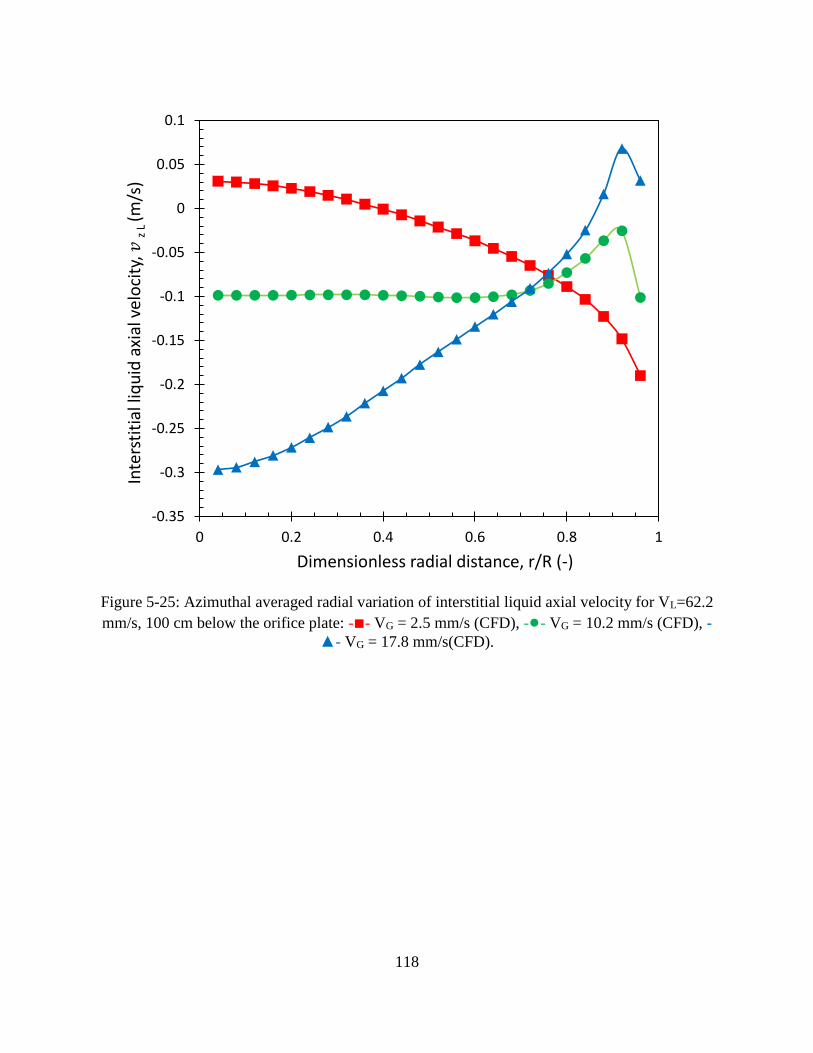
118
Figure 5-25: Azimuthal averaged radial variation of interstitial liquid axial velocity for VL=62.2
mm/s, 100 cm below the orifice plate: -■- VG = 2.5 mm/s (CFD), -●- VG = 10.2 mm/s (CFD), -
▲- VG = 17.8 mm/s(CFD).
-0.35
-0.3
-0.25
-0.2
-0.15
-0.1
-0.05
0
0.05
0.1
0 0.2 0.4 0.6 0.8 1
Inte
rsti
tial
liq
uid
axi
al v
elo
city
, 𝑣z
L (m
/s)
Dimensionless radial distance, r/R (-)

119
Figure 5-26: Azimuthal averaged radial variation of liquid axial velocity for VL=70.17 mm/s,
100 cm below the orifice plate: -■- VG = 2.5 mm/s (CFD), -●- VG = 10.2 mm/s (CFD), -▲- VG
= 17.8 mm/s(CFD).
-0.35
-0.3
-0.25
-0.2
-0.15
-0.1
-0.05
0
0.05
0.1
0 0.2 0.4 0.6 0.8 1
Inte
rsti
tial
liq
uid
axi
al v
elo
city
, 𝑣z
L (m
/s)
Dimensionless radial distance, r/R (-)
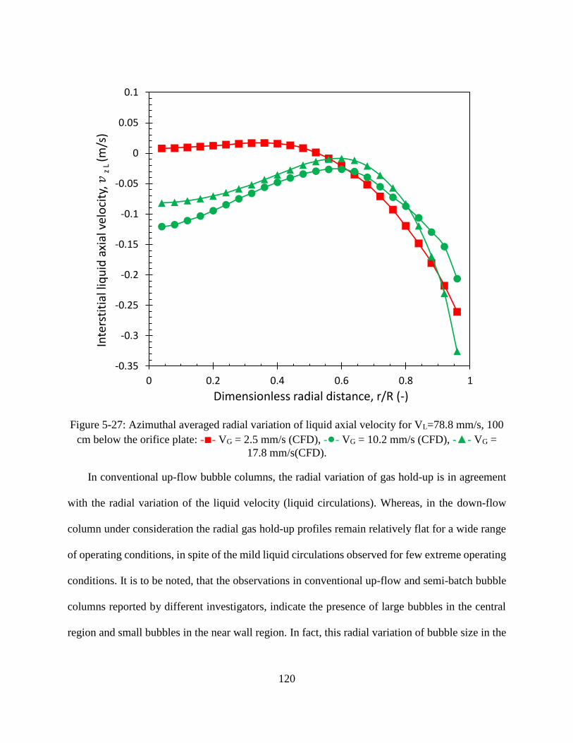
120
Figure 5-27: Azimuthal averaged radial variation of liquid axial velocity for VL=78.8 mm/s, 100
cm below the orifice plate: -■- VG = 2.5 mm/s (CFD), -●- VG = 10.2 mm/s (CFD), -▲- VG =
17.8 mm/s(CFD).
In conventional up-flow bubble columns, the radial variation of gas hold-up is in agreement
with the radial variation of the liquid velocity (liquid circulations). Whereas, in the down-flow
column under consideration the radial gas hold-up profiles remain relatively flat for a wide range
of operating conditions, in spite of the mild liquid circulations observed for few extreme operating
conditions. It is to be noted, that the observations in conventional up-flow and semi-batch bubble
columns reported by different investigators, indicate the presence of large bubbles in the central
region and small bubbles in the near wall region. In fact, this radial variation of bubble size in the
-0.35
-0.3
-0.25
-0.2
-0.15
-0.1
-0.05
0
0.05
0.1
0 0.2 0.4 0.6 0.8 1
Inte
rsti
tial
liq
uid
axi
al v
elo
city
, 𝑣z
L (m
/s)
Dimensionless radial distance, r/R (-)

121
conventional columns, is what is reflected as a radial variation in the gas hold-up which in turn
drives the liquid circulation. More specifically, the liquid circulation in the conventional up-
flow/semi-batch columns is indeed a result of the difference in the buoyancy of the centrally rising
large bubbles and near wall descending small bubbles.
Figure 5-28: Illustration of the liquid phase flow circulations encountered in a conventional up-
flow bubble column, source: (Chen et al., 1994).
Thus clearly the liquid circulations observed in conventional up-flow bubble columns is
significantly buoyancy driven. Whereas, for the down-flow bubble column under consideration
both the observation of a relatively flat radial bubble-size distribution in the microbubble range,
and flat radial gas hold-up profile; indicates that the observed liquid circulations (which is mild
and observed only in extreme operating conditions) is not buoyancy driven. Especially, in the fully
122
developed region in the downstream away from the gas sparger where only microbubbles are
present, the observed circulations (at the edge of the operating window) are more analogues to the
single-phase flow circulations of the liquid. As the drag force exerted by the liquid flow on the
microbubbles is sufficient enough to offset any buoyancy driven circulations, the microbubbles
have a very low slip velocity and so behave like suspended particles that merely follow the liquid
flow field. Based on this CFD analysis and the experimental data it could be concluded that the
liquid-circulations (for extreme operating conditions) observed in this Down-flow bubble column
is not due to the buoyancy of the micro-bubbles, but is due to the flow instabilities arising from
the upstream section of the column.
Conclusions
Experimental measurements of global gas hold-up were performed using the Phase isolation
technique and pressure drop method, axial variation of the fractional gas hold-up was measured
using the pressure transducers and radial variation of the chordal averaged hold-up was measured
using the GRD technique. Operating Regime mapping using the Drift-flux Analysis, based on
global hold-up measurements indicated that the column operating conditions are in the
homogenous regime. The measured axial and radial hold-up profiles where found to be flat. The
bubble size measurements using the high-speed camera, indicated that the mean bubble size to be
in the order of several microns (300 – 800 µm). Subsequently a 3D 3-phase Euler-Euler CFD
model was used to capture the multiphase flow dynamics for the different operating conditions.
Owing to the disparity and uncertainty in the presently available drag correlations, a drag
modification factor ′𝐷𝑓′ has been used improve the accuracy of the CFD simulations. The
formulation of ′𝐷𝑓′ takes into account both the swarm-effect (local gas holdup dependence) and

123
also the effect of the surface-active additives on the gas-liquid interface. The CFD results were
then validated using the radial chordal measurements of gas hold-up from GRD. Analysis of the
radial profiles of the interstitial liquid velocity obtained from CFD indicated 3 distinct types of
liquid flow pattern: 1) pure down-flow with no circulation 2) circulations with up-flow in the
central region and 3) circulations with up-flow near the wall region. The circulations were
observed only for the extreme operating conditions at the edge of the operating window. The
majority of the operating conditions considered (i.e. well within the operating window) exhibit
pure down-flow without any liquid re-circulations. Overall, the novelty of the gas-liquid injection
mechanism is capable of producing a high concentration (up to 54% void fraction) of micro-
bubbles (300 – 800 µm) with no liquid recirculation in a column of larger cross-section with
column diameter of 0.3 mm.

124
Chapter 6. Design Optimizations for the Novel Down Flow Bubble Column
Based on CFD
Introduction
In this chapter we discuss some of the Design optimizations proposed for the novel down-
flow bubble column. These design explorations were carried out purely based on analyzing the
hydrodynamic flow behaviors using the CFD models discussed in the previous chapters. Although
quantitatively the numerical accuracy of the CFD results may deviate from the experimental
observations, the qualitative difference in the flow predictions between the different designs
considered, helps us to arrive at the optimal design. We employed the CFD-PBM model discussed
in Chapter 4, for most of the CFD simulation setups discussed here. In addition to the existing
design feature, a new design parameter ‘Orifice Cone angle’ was considered for the orifice plate
design. For this particular design exploration, ore accurate single phase CFD simulations were
used to evaluate quantitatively the pressure drop across the orifice plate for different values of the
Orifice Cone Angle.
Perforated plate design
For the novel down-flow bubble column of 10 cm diameter with a 3-arm gas sparger located
in the top section of the column (Chapter 4), the orifice plate design involves holes of 400 µm
diameter arranged in triangular pitch of 3 mm. Here in this section we consider the effect of
changing the pitch, or the spacing between the holes. Further we explore the potential energy
savings that could be achieved by reducing the pressure drop across the orifice plate. This is made
possible by using conical holes instead of straight holes in the orifice plate.

125
6.2.1 Effect of pitch
For a fixed orifice diameter the pitch determines the percentage free are available for liquid
flow across the pore plate. So for a given superficial liquid velocity, increasing the pitch ‘P’, would
decrease the number of holes and the percentage free area, which in turn increases the jet velocity
and pressure drop across the pore plate. Four different values of pitch (P = 2, 3, 4 and 5 mm) were
considered and their performance in producing the micro-bubble dispersion is considered using
the CFD-PBM model.
Figure 6-1: Contours of interstitial liquid axial velocity for different values of orifice plate pitch
(P).

126
Figure 6-2: Contours of micro-bubble holdup for different values of orifice plate pitch (P).
The simulations were setup for the operating condition of (VG = 2mm/s and VL = 78 mm/s).
The contours of liquid axial velocity for the three different Pitch values considered is shown in
(Figure 6-1), it can be seen that for lower values of pitch the stronger jets lead to sharp velocity
gradients in the top region close to the gas sparger. The stronger jets also lead to increase in
heterogeneity and back-mixing. (Figure 6-2) shows the contours of volume fraction of the micro-
bubble in the column. It can be observed that the micro-bubble hold-up depends on the diameter
of the micro-bubbles generated. As indicated earlier, finer bubbles doesn’t necessarily translate to
increased interfacial area (ai), and that the maximum ai can be achieved only by also maximizing

127
the holdup. This explains the maximum ai value that can be observed for the pitch value of p=3mm,
which produces micro-bubbles of 284 µm leading to a holdup of 9.2%.
From the quantitative volume averaged results presented in Table 6-1, it could be noted
that increasing the pitch, leads to stronger liquid jets and hence finer micro bubbles. It should be
noted that the independent optimization of the pitch (orifice plate design), may not lead to overall
optimum operating conditions, as the optimum value of pitch also depends on the superficial
velocities (the parameters that define the operating condition). Figure 6-3 shows that the optimum
value of the pitch based on maximizing the interfacial area of the micro-bubble dispersion was
achieved for pitch = 3mm.
Table 6-1: Quantitative volume averaged results for different orifice plate pich (P).
Pitch Num of
holes
Free
area Uz jet dB
Micro-bubble
hold-up ai Kl*ai
mm - % m/s µm % m-1 hr-1
2 8947 13.9 0.6 434 8.3 1165 564.9
3 1003 1.6 5.0 284 9.2 1978 954.0
4 559 0.9 9.0 216 5.7 1591 769.3
5 361 0.6 13.9 206 2.6 749 362.5
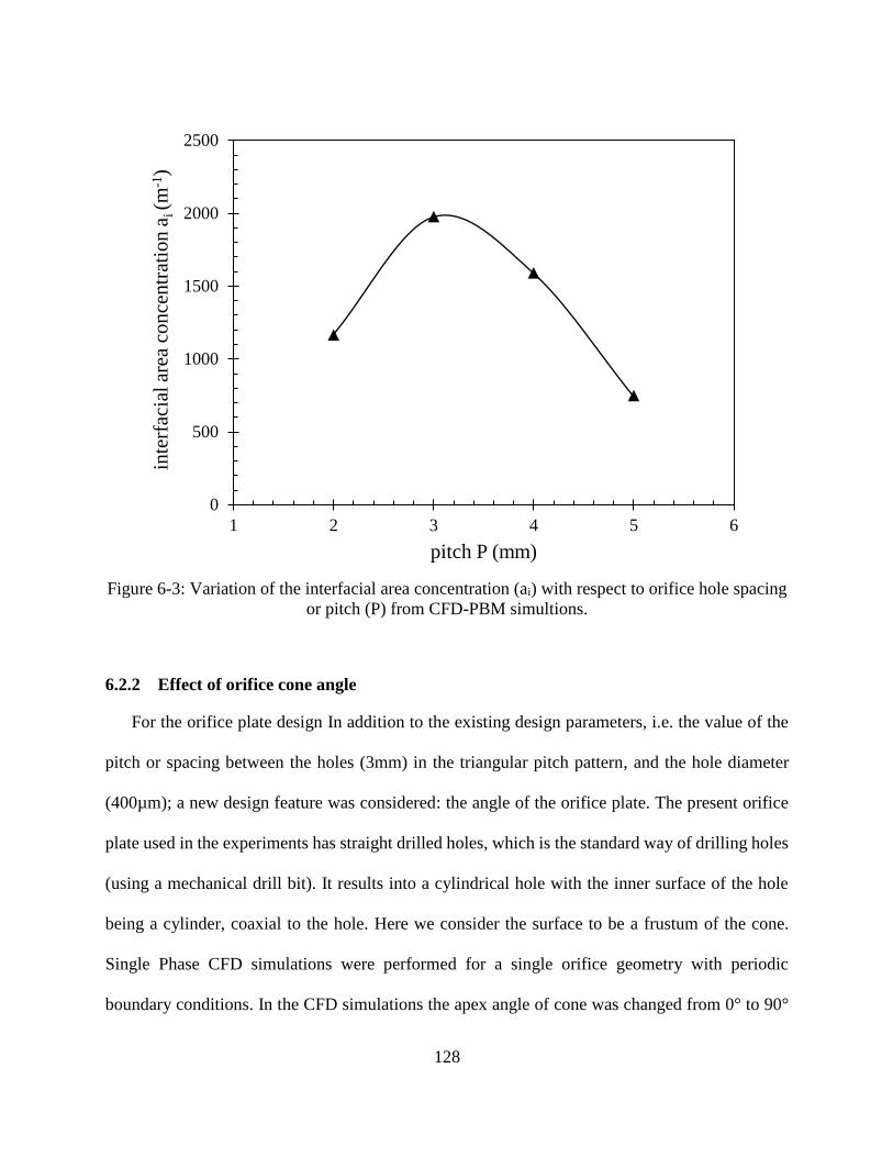
128
Figure 6-3: Variation of the interfacial area concentration (ai) with respect to orifice hole spacing
or pitch (P) from CFD-PBM simultions.
6.2.2 Effect of orifice cone angle
For the orifice plate design In addition to the existing design parameters, i.e. the value of the
pitch or spacing between the holes (3mm) in the triangular pitch pattern, and the hole diameter
(400µm); a new design feature was considered: the angle of the orifice plate. The present orifice
plate used in the experiments has straight drilled holes, which is the standard way of drilling holes
(using a mechanical drill bit). It results into a cylindrical hole with the inner surface of the hole
being a cylinder, coaxial to the hole. Here we consider the surface to be a frustum of the cone.
Single Phase CFD simulations were performed for a single orifice geometry with periodic
boundary conditions. In the CFD simulations the apex angle of cone was changed from 0° to 90°
0
500
1000
1500
2000
2500
1 2 3 4 5 6
inte
rfac
ial
area
co
nce
ntr
atio
n a
i (m
-1)
pitch P (mm)
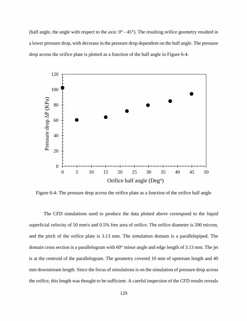
129
(half angle, the angle with respect to the axis: 0° - 45°). The resulting orifice geometry resulted in
a lower pressure drop, with decrease in the pressure drop dependent on the half angle. The pressure
drop across the orifice plate is plotted as a function of the half angle in Figure 6-4.
Figure 6-4: The pressure drop across the orifice plate as a function of the orifice half angle
The CFD simulations used to produce the data plotted above correspond to the liquid
superficial velocity of 50 mm/s and 0.5% free area of orifice. The orifice diameter is 200 micron,
and the pitch of the orifice plate is 3.13 mm. The simulation domain is a parallelepiped. The
domain cross section is a parallelogram with 60° minor angle and edge length of 3.13 mm. The jet
is at the centroid of the parallelogram. The geometry covered 10 mm of upstream length and 40
mm downstream length. Since the focus of simulations is on the simulation of pressure drop across
the orifice, this length was thought to be sufficient. A careful inspection of the CFD results reveals
0
20
40
60
80
100
120
0 5 10 15 20 25 30 35 40 45 50
Pre
ssu
re d
rop
ΔP
(K
Pa)
Orifice half angle (Dego)

130
the mechanism for the occurrence of the minimum in the pressure drop across the orifice plate.
Figure 6-5 shows the contour of the velocity magnitude at the center plane of a periodic, single
orifice geometry for 7 different orifice half angles.
Figure 6-5: The contours of liquid velocity magnitude at the center plane of CFD geometry as a
function of the orifice half angle
As the half angle is increased, the velocity maximum shifts from the entrance of the orifice to
the exit of the orifice. The Velocity maximum shifts from right at the entrance for 0° geometry to
the bottom for 45 degree geometry. The fluid has to accelerate to pass through the orifice. The
shape of the orifice hole decides the acceleration of the fluid and the pressure drop is dependent
on such acceleration. Figure 6-6 below shows the iso-surface of the velocity magnitude for the
case of 0° and 5°. Both the results are plotted for superficial liquid velocity of 93 mm/s. The
maximum velocity is 15 mm/s, and the isos-urface velocity is 15 m/s. It can be observed that the
high speed region of the jet is smaller for the 5° case. It should also be noted that the velocity
profile for the jet is very similar for both the cases hence the performance of the orifice as jet
generator is not hampered in any way. It should also be noted that the velocity inside the nozzle is
about half of that in 0° orifice. It indicates that the pressure loss reduction is achieved by smooth
acceleration of the fluid inside the 5° taper orifice hole.
θ= 0° θ= 5° θ= 15° θ= 22.5° θ= 30° θ= 37.5° θ= 45°

131
Figure 6-6: The contour of velocity magnitude overlapped with the isosurface of velocity
magnitude=15 m/s (a) orifice half angle 0°, (b) orifice half angle 5°
Figure 6-7 shows the absolute pressure along the centerline of the jets, right from the top
of the CFD domain (velocity inlet) till the bottom of the CFD domain (pressure outlet). The
upstream region is indicated by positive z values, while the jet region and downstream region is
indicated by negative z values. The origin is situated at the entrance of orifice hole. The figure
reports the data for superficial liquid velocity of 50, 78 and 93 mm/s. The maximum pressure
upstream of the orifice is always higher for 0° case. A very steep fall of the absolute pressure
should also be noted for the 0° hole. The fluid suddenly accelerates to 16 m/s from 0.05 m/s causing
abrupt pressure drop. In comparison, the pressure drop at z=0 for 5° nozzle is much less (Figure
(a)
(b)
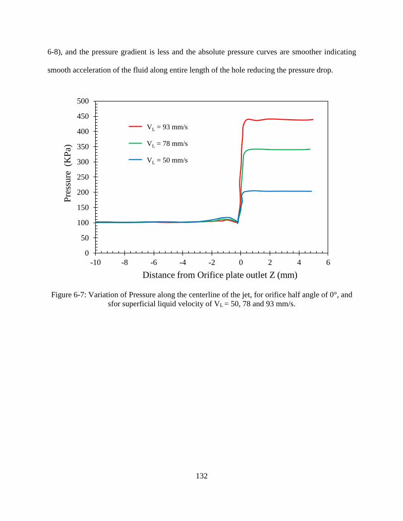
132
6-8), and the pressure gradient is less and the absolute pressure curves are smoother indicating
smooth acceleration of the fluid along entire length of the hole reducing the pressure drop.
Figure 6-7: Variation of Pressure along the centerline of the jet, for orifice half angle of 0°, and
sfor superficial liquid velocity of VL = 50, 78 and 93 mm/s.
0
50
100
150
200
250
300
350
400
450
500
-10 -8 -6 -4 -2 0 2 4 6
Pre
ssu
re (K
Pa)
Distance from Orifice plate outlet Z (mm)
Series1
Series2
Series3
VL = 93 mm/s
VL = 78 mm/s
VL = 50 mm/s

133
Figure 6-8: Variation of Pressure along the centerline of the jet, for orifice half angle of 5°, and
for superficial liquid velocity of VL = 50, 78 and 93 mm/s.
The comparison of the pressure drop across three different liquid superficial velocities VL
for the two different cases is shown in Figure 6-9. It can be observed that the pressure drop with
respect to the liquid superficial velocity/ liquid injection rate observes a parabolic trend. Further,
most importantly it could be noted that the pressure drop for 5° half angle hole is consistently
lower than the 0° half angle hole by about 30%. The holes with taper wall angle can be produced
by machining techniques like EDM (Electrical Discharge Machining) or by making a custom tool
for the job. The orifice plate made with the proposed hole design would reduce the power
requirement for all the operating superficial liquid velocities, while still producing jets of same
magnitude necessary to break the large bubbles and to achieve the target Kl*ai.
0
50
100
150
200
250
300
350
-10 -8 -6 -4 -2 0 2 4 6
Pre
ssu
re (K
Pa)
Distance from Orifice plate outlet Z (mm)
Series1
Series2
Series3
VL = 93 mm/s
VL = 78 mm/s
VL = 50 mm/s

134
Figure 6-9: The pressure drop across the orifice plate for the orifice half angle 0° and 5°
0
100
200
300
400
500
0 20 40 60 80 100
Pre
ssu
re d
rop
ΔP
(K
Pa)
Superficial liquid velocity VL (mm/s)
P(Kpa)
Series2
0o
5o

135
Gas sparger design
Figure 6-10: Illustration of the recirculation zone and Classification zone created by locating the
gas sparger in the top section of the column.
The design and location of the gas sparger determines the size of the large bubbles generated
and also the extent of the liquid recirculation in the reactor. The size of the large bubbles and the
associated rise velocity determines the extent of liquid recirculation. By moving the gas sparger to
the top, this liquid recirculation zone can be confined only to the zone above the sparger. And the
rest of the column below the sparger would have only microbubbles being carried along with the
down flowing liquid. Further, by confining the large bubbles to a minimum possible volume, the
rest of the volume of the reactor is available for accommodating the microbubbles and this
increases micro bubble holdup and the interfacial area ai. The increase in interfacial area also
results in increased overall mass transfer rate.. The large bubbles that may be carried down due to

136
strong circulation currents gets segregated from the rest of the microbubbles in the Classification
zone as shown in Figure 6-10.
6.3.1 Effect of size of injected gas bubbles
As it has been observed previous discussions, the size of the large bubbles determines
the rise velocity of the injected gas phase, and hence the extent of the recirculation generated by
this rise velocity. Further, the effectiveness of the jets in generating the microbubbles depends on
the size of the large bubbles that reach the jet zone. For these reasons, the size of the bubbles
generated by the gas sparger is a critical design parameter, and in this section we will try to get a
feel for the impact of the bubble size (of the injected gas phase) on the performance metrics of the
reactor, like the size of the micro-bubble diameter, micro-bubble holdup and Kl*ai .
In the current implementation of the CFD-PBM model, only coalescence is modelled
and for this reason there is no need for including a bin size (in the discrete PBM) that is larger than
the size of the bubbles that are being injected. At the same time for numerical consistency across
all the simulations, the discretization of the particle/bubble size space (in the PBM) has to be
maintained for the different simulations. This consistency was maintained by fixing the geometric
grid spacing for the bubble size (internal co-ordinate space), and by varying the number of bins
used. Accordingly three different values of bubble diameters: 3.4, 5.6 and 9 mm were used for the
gas phase (large bubble phase) injected through the gas sparger.
The quantitative volume averaged results for the different inlet bubble diameters is summarized in
Table 6-2. The first thing to be noted is that, the micro-bubble diameter decreases with increase in
the injected large bubble diameter. This phenomenon can be explained based on the dependence
of the breakage rate on the Weber number, which in turn is a function of the large-bubble diameter.
137
As the injected large bubble diameter increases, the bubble-weber number increases and this
increases the breakage rate (for a constant jet kinetic energy i.e. for a given plate-design and
superficial velocity). And this increase in breakage rate leads to reduces the size of the micro-
bubbles generated.
𝛺𝑏𝑟(𝑉𝑗: 𝑉𝑖) = 𝑓(𝑊𝑒𝑐𝑟𝑖𝑡,𝑊𝑒, 𝜀, … ) (6-1)
𝑊𝑒 =𝜌𝑢2𝐷𝑏𝑢𝑏
𝜎 (6-2)
The second significant trend that can be noted from Table.1 is the drastic decrease in the hold-up,
with decrease in micro-bubble diameter (columns 2 and 3 in Table.1). One may expect for an
increased performance of the reactor, especially with respect to mass transfer, by minimizing the
size of the micro-bubbles, thereby increasing the interfacial area and hence the associated mass-
transfer rate. But, this is not true as the interfacial area generated not only depends on the bubble
diameter, but also on the holdup of micro-bubbles. Although the surface area per unit volume for
a single bubble has a positive correlation with the diameter, the holdup which is a function of the
slip or rise velocity of the micro-bubbles, has a negative correlation w.r.t the diameter (for inverse
bubbly flows). So aiming to generate as small a micro-bubble as possible, will not necessarily lead
to maximum interfacial area per unit volume (ai). The finer bubbles having low slip velocity get
carried down by the liquid down-flow, thereby reducing the holdup. This explains the drastic
decrease in the hold-up, with decrease in micro-bubble diameter. The contours of liquid axial
velocity in the z-x center plane is shown in Figure 6-11. It can be seen that although higher holdup
increases interfacial area and mass-transfer rate, it also leads to increase in heterogeneity and back
mixing.

138
Table 6-2: Quantitative volume averaged results for different inlet bubble diameter Dlb.
Dlb Dsb hold-up ai Kl*ai
mm µm % m-1 hr-1
3.4 319 11.4 2161 1040
5.6 284 9.2 1978 953.99
9 224 2.5 676 326.19
Figure 6-11: Contours of Liquid axial for different inlet bubble diameter Dlb.
Dlb = 3.4 mm Dlb
= 5.6 mm Dlb
= 9 mm

139
6.3.2 Effect of inlet-gas distribution
In addition to relocating the sparger, different sparger configurations were also considered
to compare their effect on the length of the Classification zone. Figure 6-12 shows the source point
representation of the different sparger configurations considered.
Figure 6-12: Source point representation of the 3 different sparger configurations.
The three-arm sparger is the present design used in the current experimental setup. We
compare the circulation patterns generated by this sparger with two other sparger configurations.
The spider sparger is designed with the intention to uniformly introduce the large bubbles across
the cross-section of the column. Whereas the central sparger concentrates the release of the large
bubbles in a central disc. Here we are interested only in the qualitative difference between the
liquid re-circulations encountered in these three different design configurations.
Central Sparger Spider Sparger 3 arm Sparger
2.5 cm 10.16 cm

140
Figure 6-13: Contours of large bubble holdup for different sparger configurations.
Figure 6-14: Contours of micro bubble holdup for different sparger configurations.
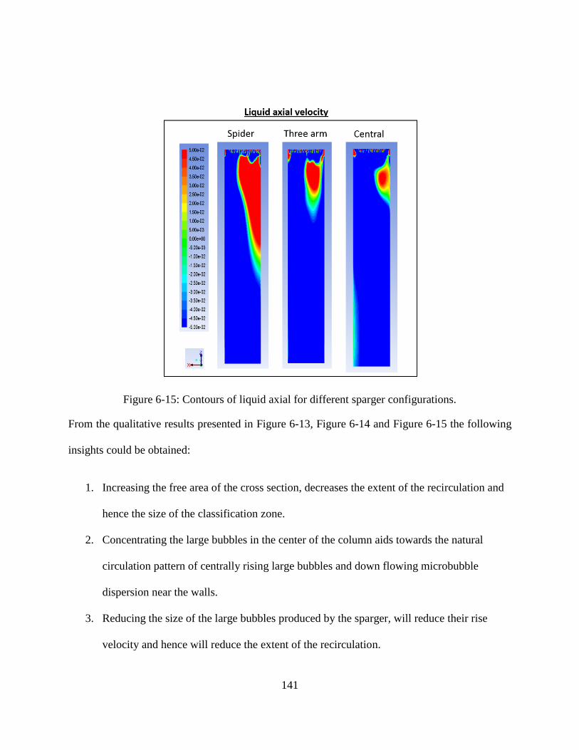
141
Figure 6-15: Contours of liquid axial for different sparger configurations.
From the qualitative results presented in Figure 6-13, Figure 6-14 and Figure 6-15 the following
insights could be obtained:
1. Increasing the free area of the cross section, decreases the extent of the recirculation and
hence the size of the classification zone.
2. Concentrating the large bubbles in the center of the column aids towards the natural
circulation pattern of centrally rising large bubbles and down flowing microbubble
dispersion near the walls.
3. Reducing the size of the large bubbles produced by the sparger, will reduce their rise
velocity and hence will reduce the extent of the recirculation.
142
Conclusions
In this work we have presented the possibility of driving Design explorations and
optimizations purely based on CFD models. By using the CFD-PBM model to compare the
qualitative difference for different design configurations we were able to arrive at optimum values
for existing design parameters or features like the pitch or spacing of the holes in the orifice plate
and the desired diameter of the injected large bubbles from the gas sparger. We also, discovered
that by injecting the mm sized large bubbles from a concentrated location in the center of the
column for the sparger located in the top section of the column yields in minimal liquid re-
circulations, there by extending the length of homogeneous flow section in the downstream section
of the column. In addition to these multiphase simulations, single phase simulations setup using a
periodic domain for a single orifice in the orifice-plate, suggested the potential for decreasing the
pressure drop across the orifice plate, by using conical holes instead of straight holes. Further,
CFD analysis found that the optimum value of the half angle of the conical holes to 5o , for which
the maximum pressure drop was observed. From quantitative analysis of the single phase
simulations, it was estimated that the conical hole with 5o conical holes consistently outperforms
the straight hole design for all values of liquid injection rates (VL = 50, 78 and 93 mm/s), by
achieving a 30% reduction in pressure drop. This 30% reduction in pressure drop in turn translates
to increase in energy savings by decreasing g the energy required for maintaining the liquid
injection rate.

143
Chapter 7. One Dimensional Performance Model
Introduction
Although 1D models lack the accuracy and flow details that a 3D CFD model provides,
they are still attractive for their simplicity and ability to give quick estimates for design
considerations. In this chapter we review one such existing approach based on Drift-flux
modelling. Later we derive a 1D performance model to estimate the performance of any given
column of arbitrary length. This performance model is geared more towards providing rough
estimates for scale-up purposes, provided the considered design preserves the efficiency of the
bubble generation mechanism and extent of the liquid phase circulations is maintained over the
scale-up process.
Drift flux model
For conventional bubble columns the two phase gas-liquid flows have been extensively
studied with the help of Drift flux models. The concept of Drift flux was introduced by (Wallis,
1969). The drift flux VGL is defined as the superficial velocity of the dispersed phase (gas) with
respect to the average velocity of the mixture phase.
𝑉𝐺𝐿 = 𝑉𝐺 − 𝜖𝐺 (𝑉𝐺 + 𝑉𝐿 ) (3)
A plot of VGL versus the gas holdup 𝜖𝐺 can be used to identify the operating regime and also to
identify regime transitions between homogeneous and heterogeneous regimes (Joshi et al., 1990).
Homogenous regime is characterized by a uniform holdup profile across the cross-section of the
column with a narrow bubble size distribution. Heterogeneous regime is characterized by a non-

144
uniform holdup profile and recirculation of the continuous phase (liquid). Thus, the drift flux plots
were used to identify the operating regime of the bubble columns, without the need for a radial
measurement of the holdup profile. For columns operated in the heterogeneous regime, Zuber &
Findlay (1965) came up with the following model to predict the relationship between the average
gas hold-up ⟨∈𝐺⟩ and superficial velocity.
𝑉𝐺⟨∈𝐺⟩
= 𝐶0(𝑉𝐺 + 𝑉𝐿) + 𝐶1 (4)
Where,
𝐶0 = ⟨∈𝐺 (∈𝐺 𝑢𝐺 +∈𝐿 𝑢𝐿)⟩
⟨∈𝐺⟩ (𝑉𝐺 + 𝑉𝐿 ) 𝑎𝑛𝑑 𝐶1 =
⟨∈𝐺 ∈𝐿 𝑉𝑆⟩
⟨∈𝐺⟩
(5)
7.2.1 3-phase drift flux model
Let’s consider a differential element of thin disc at a given plane in the fully developed,
predominantly 1D flow region. And for simplicity let’s derive the drift flux equation for one of the
dispersed phases (large bubbles) with respect to the mixture, then the same could be
extended to the other dispersed phases (small bubbles). Let the subscript ‘G’ denote
large-bubbles phase, ‘g’ denote small-bubbles phase; and ‘L’ denote the liquid phase. From the
definition of the slip velocity, the slip velocity of large bubbles could be defined as:
𝑉𝑆𝐺 = 𝑢𝐺 − 𝑢𝐿 (6)
Where 𝑢𝐺 and 𝑢𝐿 are the interstitial velocity of the Large bubbles phase and liquid, so from the
definition of the superficial velocity, it can be written that:

145
𝑉𝑆𝐺 =
𝑉𝐺𝜖𝐺−𝑉𝐿𝜖𝐿 (7)
Now, rearranging and area averaging on both sides:
⟨𝑉𝐺⟩ = ⟨ 𝜖𝐺𝑉𝐿𝜖𝐿 ⟩ + ⟨𝜖𝐺 𝑉𝑆𝐺⟩ (8)
Dividing on both sides by ⟨𝜖𝐺⟩
⟨𝑉𝐺⟩
⟨𝜖𝐺⟩ =
⟨ 𝜖𝐺𝑉𝐿𝜖𝐿 ⟩
⟨𝜖𝐺⟩ +
⟨𝜖𝐺 𝑉𝑆𝐺⟩
⟨𝜖𝐺⟩ (9)
Now, multiplying and dividing the first term on the L.H.S by the mixture superficial velocity
⟨𝑉⟩ = ⟨𝑉𝐺⟩ + ⟨𝑉𝑔⟩ + ⟨𝑉𝐿⟩ :
⟨𝑉𝐺⟩
⟨𝜖𝐺⟩ =
⟨ 𝜖𝐺𝑉𝐿𝜖𝐿 ⟩
⟨𝜖𝐺⟩ ⟨𝑉⟩ ⟨𝑉⟩ +
⟨𝜖𝐺 𝑉𝑆𝐺⟩
⟨𝜖𝐺⟩ (10)
Further, from mass balance of gas: ⟨𝑉𝐺⟩ = −⟨𝑉𝑔⟩ and so ⟨𝑉⟩ = ⟨𝑉𝐿⟩.

146
By replacing the point superficial velocity 𝑉𝐿 in terms of the interstitial velocity (𝑉𝐿 = 𝜖𝐿 𝑢𝐿 ) and
for brevity let’s drop the ⟨ ⟩ for the area averaged superficial velocities:
𝑉𝐺⟨𝜖𝐺⟩
= 𝐶0,𝐺 𝑉𝐿 + 𝐶1,𝐺 (11)
Where, 𝐶0,𝐺 = ⟨𝜖𝐺 𝑢𝐿⟩
⟨𝜖𝐺⟩ 𝑉𝐿 and 𝐶1,𝐺 =
⟨𝜖𝐺 𝑉𝑆𝐺⟩
⟨𝜖𝐺⟩ (12)
Similarly, for the small bubbles phase the drift-flux equation is:
𝑉𝑔⟨𝜖𝑔⟩
= 𝐶0,𝑔 𝑉𝐿 + 𝐶1,𝑔 (13)
Where, 𝐶0,𝑔 = ⟨𝜖𝑔 𝑢𝐿⟩
⟨𝜖𝑔⟩ 𝑉𝐿 and 𝐶1,𝑔 =
⟨𝜖𝑔 𝑉𝑆𝑔⟩
⟨𝜖𝑔⟩ (14)
Although these drift flux models are complete and do not have any gross-assumptions over
the conventional drift-flux model for two-phase, they still need high-resolution holdup and
interstitial velocity data, which is hard to obtain from experiments. Nevertheless, this high-
resolution data can be obtained from carefully and reliably simulated CFD results that agree with
the global measurements from experiments. And such data can be used to evaluate the constants
𝐶0,𝐺 , 𝐶1,𝐺 , 𝐶0,𝑔 , 𝐶1,𝑔 .
147
7.2.2 Simplified 3-phase drift flux model
Extensive 3D CFD simulation for all superficial velocities and subsequent fine tuning of
the closure parameters in the Euler-Euler CFD and PBM models is time consuming, so in order to
exploit the Experimental data obtained from the full range of superficial velocities (VG = 2 - 10
mm/s and VL = 78 - 93 mm/s), we need a simplified drift-flux model, that at the same time can
treat the large and small bubbles as separate phases (difference in the large and small bubble slip
velocities) and also one that can consider the holdup of large (єG)and small bubbles (єg) separately
and not as a lumped parameter (α = єG +єg). To this end, let’s reconsider the definition of slip
velocity, only this time we will assume that the there is no radial holdup profile and the definition
of the slip velocity for the differential element holds good for the entire cross section. Or in another
way, it’s equivalent to considering an average slip velocity for each phase (large bubbles and small
bubbles) and an average holdup that results from a slight holdup profile. Although this may not be
true, as there is a clear radial segregation of large and small bubbles, we will proceed forward for
the case of simplicity.
𝑉𝑆𝐺 =
𝑉𝐺𝜖𝐺−𝑉𝐿𝜖𝐿 (15)
𝑉𝑆𝑔 =
𝑉𝐺𝜖𝑔−𝑉𝐿𝜖𝐿 (16)
Where, 𝜖𝑔 + 𝜖𝐺 + 𝜖𝐿 = 1 and 𝜖𝑔 + 𝜖𝐺 = 𝛼
From Experimental data, for 36 different combinations of 𝑉𝐺 𝑎𝑛𝑑 𝑉𝐿 in the range of (VG = 2 to 10
mm/s and VL = 78 to 93 mm/s), we have exact measurements of the small bubble diameters in the
range of 150 to 250 µm. Further we could assume the large bubble diameter to be in the range of

148
20mm. With these values as a priori, let’s consider the empirical slip velocity correlation from
(Clift et al., 1978) as a good approximation for determining the slip velocities 𝑉𝑆𝐺 𝑎𝑛𝑑 𝑉𝑆𝑔.
Figure 7-1: Rise velocity for a single bubble in air-water system from (Clift et al., 1978)
The piecewise polynomial fit for the contaminated rise velocity from Figure 7-1 is given below:
Vs = 4.8e-9*dB5 + 9.46e-6* dB
4 - 1.29e-2* dB3
+ 0.52* dB2 + 0.17* dB + 165.61 for (dB > 3.4 mm)
Vs = -2.62* dB5 + 24.2* dB
4 - 76.3* dB3
+ 71.7* dB2 + 86.79* dB, for (dB < 3.4 mm)
(17)
Now, 𝑉𝑆𝐺 𝑎𝑛𝑑 𝑉𝑆𝑔 could be obtained from the piece-wise polynomial fit. Then the two slip velocity
equations (15) and (16) have only two unknowns 𝜖𝑔 𝑎𝑛𝑑 𝜖𝐺 , which could be solved for and the
gas holdup 𝛼=(𝜖𝑔 + 𝜖𝐺) can be determined for a given 𝑉𝐺 𝑎𝑛𝑑 𝑉𝐿. Figure 7-2 shows the parity plot
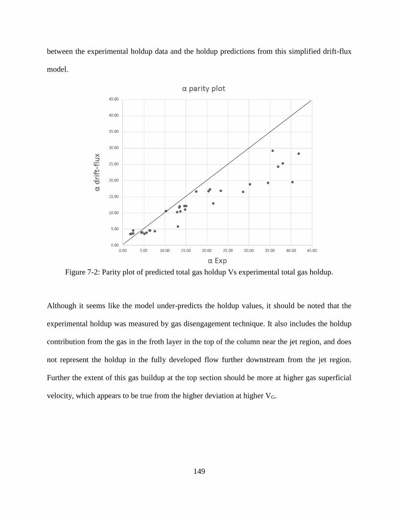
149
between the experimental holdup data and the holdup predictions from this simplified drift-flux
model.
Figure 7-2: Parity plot of predicted total gas holdup Vs experimental total gas holdup.
Although it seems like the model under-predicts the holdup values, it should be noted that the
experimental holdup was measured by gas disengagement technique. It also includes the holdup
contribution from the gas in the froth layer in the top of the column near the jet region, and does
not represent the holdup in the fully developed flow further downstream from the jet region.
Further the extent of this gas buildup at the top section should be more at higher gas superficial
velocity, which appears to be true from the higher deviation at higher VG.

150
Table 7-1: Gas hold-up predictions from the drift-flux model for the flow conditions encountered
in the down flow bubble column with column diameter of 10 cm.
VG VL
Gas holdup
Exp CFD-PBM Drift –flux
(Clift rise-velocity)
mm/s mm/s % % %
2.06 78 6.3 6.0 4.6
2.06 93 2.0 4.9 3.6
6.17 78 14.6 10.0 12.1
6.17 93 13.7 7.8 10.6
10.3 78 25.6 8.9 18.8
10.3 93 20.4 9.6 16.7
1D performance model
The objective for developing a performance model is to predict the length of a reactor required
to achieve a given conversion/ absorption of gas in the liquid phase. The model needs to be simple
and must be able to provide quick results in terms of the liquid concentration of the dissolved
species and the axial variation of the bubble size due to mass-transfer, hydro-static pressure and
surface tension effects (Laplace pressure). The model must also be in terms of relatable parameters,
whose values can be obtained from the higher fidelity CFD-PBM models that were discussed in
the earlier sections. The model should also be extensible to account for reactions involving the
dissolved species in the continuous phase (liquid).

151
Figure 7-3Illustration of the shell balance approach used for the 1D performance model
For the cases with the sparger at the top section of the column, the flow below the sparger
consists only of the micro-bubble dispersion in the liquid phase. Hence it makes more sense to use
a 1D performance to model the section below the sparger for these cases. The performance model
was derived by considering a differential shell of width dZ as shown in figure Figure 7-1, and
taking the mass balance of the gas phase and for an arbitrary dissolved species ‘i’ in the liquid
phase.
Following phenomenon are accounted for in the derivation:
1. Axial dispersion of the dissolved species in the liquid side
2. Interphase mass transfer from gas to liquid.
3. Effect of Laplace pressure on the bubble size.
4. Effect of Hydrostatic pressure on the bubble size.
VL|Z=0
VG, N
B
NG|Z=0
NG|z
NG|z+dz
+dZ
P|Z=0
dB|Z=0
152
And the following assumptions are made:
1. Only one class of down flowing micro bubbles are considered, and hence can be used for
modelling the section below the gas sparger
2. Coalescence or breakup of bubbles is neglected.
3. Axial dispersion of bubbles is neglected, and further it is assumed that the radial holdup
profile remains constant axially, i.e. C0 and C1 remain constant for the entire length of
the reactor.
4. The decrease in size of the bubbles is only due to Hydrostatic pressure, Laplace pressure
and Mass transfer
7.3.1 Nomenclature used in the 1 D performance model
𝐶𝑖∗ Component i concentration at the interface, mol/m3
𝐶𝑖 Component i concentration in bulk liquid, mol/m3
𝐷𝑖 Component i Diffusivity of gas in liquid, m2/s
𝐷𝐿 Axial dispersion coefficient for liquid, m2/s
𝑛𝐵 Number of bubbles entering the domain per second, 1/s
𝑁𝑖 Molar flow rate of component i in the gas phase, kmol/s
𝑁𝐺 Molar flow rate of gas phase, kmol/s
𝑉𝑠 Slip velocity, m/s
𝑉𝐿 Liquid superficial velocity, m/s
𝑉𝐺 Gas superficial velocity, m/s
153
𝑎𝑖 Interfacial area concentration, m2/m3
𝑑𝐵 Bubble diameter, m
𝑘𝑖 Liquid side mass transfer coefficient from Component i gas to liquid, m/s
𝑝𝑔 Partial pressure of gas specie, Pa
𝐻𝑒𝑖 Henry’s law constant for Component i, mol/(m3.Pa)
𝑦𝑖 Mole fraction of component I in the gas phase
𝑃 Total pressure inside the bubble at height z, Pa
𝑅 Universal gas constant, 8.314 J/(mol.K)
𝐴𝐶 Cross sectional area of the column, m2
𝑇 Temperature, K
𝑔 Gravitational acceleration, m/s2
𝑧 Vertical coordinate, m
∈𝐺 Local gas volume fraction at height z, -
∈𝐿 Local liquid volume fraction at height z, -
𝜌𝐿 Density of liquid, kg/m3
𝜌𝐺 Density of gas, kg/m3
𝜎 Surface tension, N/m

154
The equation describing the transport of dissolved species in liquid phase including turbulent
dispersion is given as :
𝒟𝐿𝑑2𝐶𝑖𝑑𝑧2
− 𝑉𝐿𝑑𝐶𝑖𝑑𝑧
+ 𝑘𝑖 ∙ 𝑎𝑖 ∙ (𝐶𝑖∗ − 𝐶𝑖) + 𝑆𝑖 = 0
(18)
The pressure 𝑃 inside the bubbles at height Z is defined as the summation of the pressure at z=0,
and the hydrostatic pressure due to the column of gas-liquid dispersion of height z and the Laplace
pressure.
𝑃 = 𝑃|0 + 𝜖�̅� ∙ 𝜌𝐿𝑔𝑧 +4𝜎
𝑑𝐵 (19)
Liquid density is used instead of mixture density since the gas density is negligible compared to
the liquid. The height averaged volume fraction of liquid is given by:
𝜖�̅� =1
𝐴𝐶 ∙ 𝑧∫ 𝜖𝐿 ∙ 𝐴𝐶 ∙ 𝑑𝑧𝑧
0
=1
𝑧∫ 𝜖𝐿 ∙ 𝑑𝑧𝑧
0
(20)
Substituting this in Eq. 3 and taking derivative of pressure w.r.t. z:

155
𝑑
𝑑𝑧𝑃 =
𝑑
𝑑𝑧(1
𝑧∫ 𝜖𝐿 ∙ 𝑑𝑧𝑧
0
∙ 𝜌𝐿𝑔𝑧) +𝑑
𝑑𝑧(4𝜎
𝑑𝐵) (21)
𝑑
𝑑𝑧𝑃 = 𝜌𝐿𝑔
𝑑
𝑑𝑧(𝑧
𝑧∫ 𝜖𝐿 ∙ 𝑑𝑧𝑧
0
) + 4𝜎𝑑
𝑑𝑧(1
𝑑𝐵) (22)
𝑑
𝑑𝑧𝑃 =
𝑑
𝑑𝑧(1
𝑧∫ 𝜖𝐿 ∙ 𝑑𝑧𝑧
0
∙ 𝜌𝐿𝑔𝑧) +𝑑
𝑑𝑧(4𝜎
𝑑𝐵) (23)
𝑑𝑃
𝑑𝑧= 𝜖𝐿𝜌𝐿𝑔 −
4𝜎
𝑑𝐵2
𝑑(𝑑𝐵)
𝑑𝑧 (24)
The mole balance for ith component in the gas phase is:
𝑑𝑁𝑖𝑑𝑧
= −1 ∙ 𝑘𝑖 ∙ 𝑎 ∙ (𝐶𝑖∗ − 𝐶𝑖) ∙ 𝐴𝐶 (25)
The total molar flow rate for gas NG is given by:s
𝑁𝐺 =∑ 𝑁𝑖
𝑛
𝑖=1
(26)
Volumetric flow rate of Gas is:
𝑄𝐺 =𝑛𝐵𝜋𝑑𝐵
3
6 (27)
Also,

156
𝑄𝐺 =𝑁𝐺𝜌𝐺
(28)
Which gives,
𝑑𝐵3 =
6𝑁𝐺𝑛𝐵𝜌𝐺𝜋
(29)
𝑑𝐵3 =
6𝑁𝐺𝑅 𝑇
𝑛𝐵𝑃𝜋 (30)
𝑑𝐵 = (6𝑁𝐺𝑅 𝑇
𝑛𝐵𝑃𝜋)
13 (31)
𝑑𝐵 = (6𝑅 𝑇
𝑛𝐵𝜋)
13 (𝑁𝐺𝑃)
13 (32)
𝑑(𝑑𝐵)
𝑑𝑧 = (
6𝑅 𝑇
𝑛𝐵𝜋)
13 𝑑
𝑑𝑧 ( (
𝑁𝐺𝑃)
13) (33)
𝑑(𝑑𝐵)
𝑑𝑧 = (
6𝑅 𝑇
𝑛𝐵𝜋)
13 (1
3) (
𝑁𝐺𝑃)−23 [𝑁𝐺′𝑃 + 𝑁𝐺𝑃
′
𝑃2] (34)
Substituting (6) in (4) we get:
𝑑(𝑃)
𝑑𝑧= [𝜖𝐿𝜌𝐿𝑔 −
4𝜎
𝑑𝐵2
1
3(6𝑅 𝑇
𝑛𝐵𝜋)
1
3
(1
3) (
𝑁𝐺
𝑃)−2
3 [𝑁𝐺′ 𝑃 + 𝑁𝐺𝑃
′
𝑃2]] (35)

157
𝑑(𝑃)
𝑑𝑧+ [4𝜎
𝑑𝐵2
1
3(6𝑅 𝑇
𝑛𝐵𝜋)
1
3
(1
3) (
𝑁𝐺
𝑃)−2
3 (𝑁𝐺𝑃
′
𝑃2)]
= [𝜖𝐿𝜌𝐿𝑔 −4𝜎
𝑑𝐵2
1
3(6𝑅 𝑇
𝑛𝐵𝜋)
1
3
(1
3) (
𝑁𝐺
𝑃)−2
3 [𝑁𝐺′
𝑃]]
(36)
𝑑(𝑃)
𝑑𝑧=
[𝜖𝐿𝜌𝐿𝑔 −4𝜎𝑑𝐵213 (6𝑅𝑇𝑛𝐵𝜋
)
13(𝑁𝐺𝑃 )
−23(1𝑃)(
𝑑𝑁𝐺𝑑𝑧
)]
[1 +4𝜎𝑑𝐵213 (6𝑅𝑇𝑛𝐵𝜋
)
13(𝑁𝐺𝑃 )
−23 (𝑁𝐺𝑃2)]
(37)
Also, the equation describing the transport of dissolved species in liquid phase is given by:
𝑑𝑁𝑖𝑑𝑧
= −1 ∙ 𝑘𝑖 ∙ 𝑎𝑖 ∙ (𝐶𝑖∗ − 𝐶𝑖) ∙ 𝐴𝐶 (38)
Where, the species concentration at the interface is defined by the Henry’s law using the gas partial
pressure inside the bubble.
𝑪𝒊∗ = 𝑦𝑖. 𝑃. 𝐻𝑒𝑖 (39)
Where, 𝑦𝑖 =𝑁𝑖
𝑁𝐺 and for a pure gas the partial pressure is equal to the total pressure inside bubble.
Where the total molar flow rate of gas 𝑁𝐺 is given by:

158
𝑁𝐺 =∑ 𝑁𝑖
𝑛
𝑖=1
(40)
The differential equations (18),(37) and (38) together represent the performance model. It is to be
noted that equation (18) is a second order ODE and can be rearranged as a system of two first order
ODEs. There is only one independent variable z, and the rest of them (𝐶𝑖, 𝑁𝑖 and 𝑃) are dependent
variables. The ODEs are solved using a ‘bvp4c’ boundary value solver in MATLAB for a given
length of the reactor. The details of the MATLAB files with the boundary value problem setup is
given in Apendix-C. In addition to these ODEs the following algebraic equations are solved at
each iteration.
1. Bubble diameter, 𝑑𝐵:
𝑑𝐵 = (6𝑁𝐺𝑅𝑇
𝜋𝑛𝐵𝑃)1/3
(41)
2. Gas superficial velocity, 𝑉𝐺:
𝑉𝐺 is calculated using 𝑑𝐵 and nB as:
𝑉𝐺 =𝑛𝐵𝜋6 𝑑𝐵
3
𝐴𝐶 (42)
2. Mass transfer coefficient, 𝑘𝑖:
The mass transfer coefficient can be related to the bubble diameter using the Sherwood number,
defined as:

159
𝑆ℎ =𝑘𝑖 ∙ 𝑑𝐵𝐷𝑖
(43)
Rearranging,
𝑘𝐿 =𝑆ℎ ∙ 𝐷𝑖𝑑𝐵
(44)
The Sherwood number is assumed to be a constant which is 2 for diffusion controlled regime.
3. The interfacial area concentration, 𝑎𝑖:
The interfacial area concentration for given bubble diameter and gas volume fraction is given by:
𝑎𝑖 =6 ∈𝐺𝑑𝐵
(45)
To calculate 𝑎𝑖 , the value of ∈𝐺 is required and is calculated using the drift flux model.
4. Drift flux model for gas volume fraction, ∈𝐺:
The volume fraction of gas is calculated using the 1-D drift flux model. The drift flux equation is
written as:
𝑉𝐺⟨∈𝐺⟩
= 𝐶0(𝑉𝐺 + 𝑉𝐿) + 𝐶1 (46)
⟨∈𝐺⟩ = 𝑉𝐺
𝐶0(𝑉𝐺 + 𝑉𝐿) + 𝐶1 (47)

160
Only two phases are considered (only small, down flowing bubbles are modelled). The following
constraint on volume fractions is used: ∈𝐺+∈𝐿= 1. C0 and C1 are the drift flux constants and
depend on the superficial gas and liquid velocity, bubble diameter, fluid property and column
geometry.
7.3.2 A test case solution
The following test case was setup for a down-flow bubble column of 1 m2 cross-sectional
area and length of 4m. The gas phase was considered to be made of only two are components (O2
and N2) and their dissolution in the liquid phase (water) was modelled. Subscripts ‘1’ and ‘2’
denote O2 and N2 respectively. Values for the constants were chosen based on the physical
properties of Oxygen and Nitrogen.
Table 7-2: Values of the input parameter and constants used in the test case for the 1D
performance model.
R = 8.314 J/(mol.K)
T = 298 K
𝐷𝐿 = 2.10E-09 m2/s
He1 =1.283E-05 mol/(Pa.m3)
D1 = 2.10E-09 m2/s
Sh = 5
Ac = 1 m2
𝑉𝐺|𝑧=0 = 0.001 m/s
𝑉𝐿|𝑧=0 = 0.06 m/s
𝑑𝐵|𝑧=0=0.00022 m.
He2 =6.415E-05 mol/(Pa.m3)
D2 = 2.10E-09 m2/s
𝐷𝑡𝑢𝑟𝑏,𝐿= 0.001 m2/s
C0=1
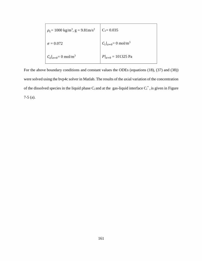
161
𝜌𝐿= 1000 kg/m3, g = 9.81m/s2
𝜎 = 0.072
𝐶2|𝑧=0= 0 mol/m3
C1= 0.035
𝐶1|𝑧=0= 0 mol/m3
𝑃|𝑧=0 = 101325 Pa
For the above boundary conditions and constant values the ODEs (equations (18), (37) and (38))
were solved using the bvp4c solver in Matlab. The results of the axial variation of the concentration
of the dissolved species in the liquid phase Ci and at the gas-liquid interface Ci
* , is given in Figure
7-5 (a).

162
Figure 7-4: Axial variation of: (a) Liquid side concentration of Oxygen - C1 , (b) Nitrogen - C2
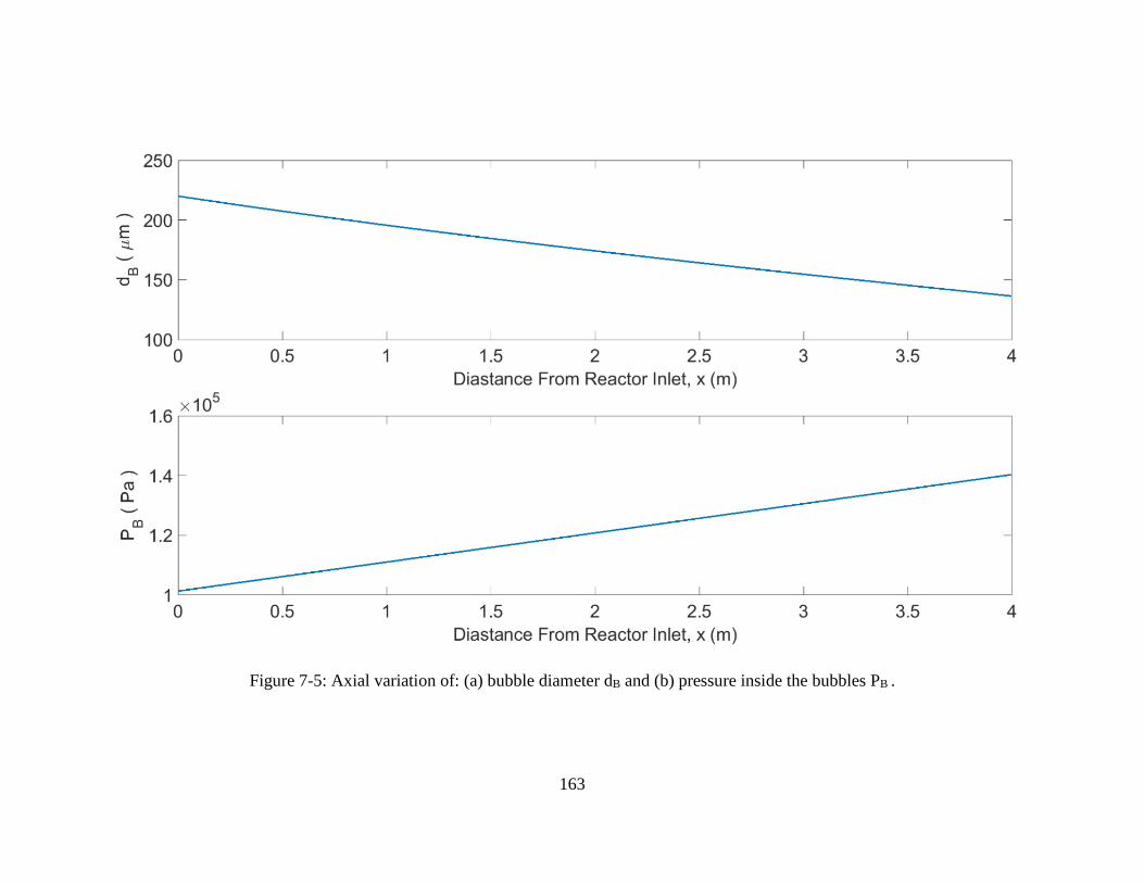
163
Figure 7-5: Axial variation of: (a) bubble diameter dB and (b) pressure inside the bubbles PB .
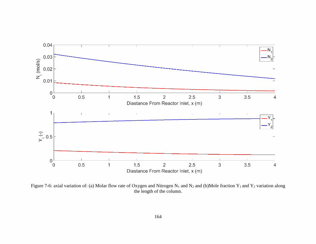
164
Figure 7-6: axial variation of: (a) Molar flow rate of Oxygen and Nitrogen N1 and N2 and (b)Mole fraction Y1 and Y2 variation along
the length of the column.

165
Conclusions
The significance of the Drift-flux model in one dimensional multiphase flows in relating
the gas and liquid superficial velocities VG and VL to the average gas hold-up was discussed.
Further for situations with a radial gas hold-up profile the significance of the drift-flux constants
C0 and C1 and the expressions to evaluate the constants were discussed. It was showed that the
values of C0 and C1 can be obtained from high resolution flow measurements of local gas hold-up
or from a validated CFD simulation. Subsequently a one dimensional performance model for a
column of arbitrary length was derived to capture the dissolution of the gas phase consisting of
more than one chemical components in the liquid phase. The modelling of the interphase-mass
transfer from the gas to liquid phase and the axial-dispersion of the dissolved species in the liquid-
phase was also considered. Further, the effect of variation of the bubble size due to the hydrostatic
pressure, Laplace pressure and mass-transfer; were also incorporated into the derivation of the 1D
performance model. Finally, the 1D performance model was solved using a boundary value solver
‘bvp4c’ in MATLAB, for a test case of Oxygen dissolution from gas phase (mixture of O2 and N2)
in to liquid phase in a column of length 4m. The one dimensional model is capable of capturing
the axial variation in the bubble size, pressure inside the bubble and the concentration of the
different chemical components in both the gas and liquid phase.

166
Chapter 8. Summary
In conclusion, we summarize some of the key contributions of this work.
Sigmoid function based drag modification for capturing the plunging liquid jet action
in a Euler-Euler framework
The present CFD models and approaches used for simulating the phenomena of a plunging
liquid jet in a pool of liquid was reviewed and the existing difficulties in modelling all three
sections of a plunging jet bubble column in a single CFD simulation was highlighted. The inability
of the existing the drag-law formulations in the Euler-Euler framework to capture the gas
entrainment action of the plunging liquid jet was pointed out, and a sigmoid function based drag
modification function was proposed to resolve the problem. The successful implementation of the
proposed drag modification function enabled the CFD simulations to reliably reproduce the
experimentally observed free-jet lengths and also the gas hold-up in the two-phase bubbly flow
region in the downstream section of the column. We showed that the high resolution three
dimensional flow filed and turbulence data obtained from the CFD simulations, could be further
utilized for performing a linear stability analysis to calculate the critical gas hold-up at which the
regime transition from homogeneous to heterogeneous regime takes place.
A force-balance based method for obtaining the optimum drag-modification function
for simulating bubbly-flows
The list of drag correlations (Table 2-1) and also the proposed drag modifications based on
local gas holdup (Table 2-2) currently available in the literature were reviewed in Chapter 2. It was
observed that these correlations vary widely in their formulations and also applicability for
different ranges of bubbly flow in terms of the bubble size and the gas-liquid system. To overcome
this difficulty in choosing the appropriate formulation for modelling the drag coefficient cD , we

167
have made use of a simple force-balance based method to compare the predictions of the different
drag correlations and also to come up with optimum correction/ modification functions for each
one of those drag correlations considered. The force-balance method (section 5.3) involves
balancing the drag force to the buoyancy force, and then comparing the average slip velocity
predictions from the model to that of the experimentally observed values. The drag modification
function obtained from such a force-balance method (Table 5-1) was used to simulate the flow
conditions in the novel down-flow bubble column of large cross-section.
Nature of liquid circulations encountered in a down-flow bubble column of large
cross-section
In conventional up-flow and semi-batch bubble columns, the liquid phase re-circulation is
driven by the presence of large bubbles in the center and the small bubbles close to the wall. The
presence of this radial variation in the bubble size and the gas hold-up, leads to significant
difference in the local buoyancy force experienced by the gas phase or bubble swarms. This
difference in buoyancy, drives the liquid phase recirculation in these conventional bubble columns.
Both the experimental data and the validated CFD results from the simulations for the novel down
flow bubble column of 30 cm diameter (Chapter 5), indicated a flat radial gas hold-up profile and
mean bubble size and no liquid phase recirculation. This lead to the conclusion that the nature of
the flow circulations encountered in the down-stream section of the novel down flow bubble
column are not buoyancy driven as in the case of the conventional bubble columns (section 5.5.4),
and that the microbubbles have a very low slip velocity and so behave more like suspended
particles that merely follow the liquid flow field.

168
Orifice-plate and gas sparger design for maximizing performance of the novel down-
flow bubble column
Based on single phase CFD simulations in a periodic domain (section 6.2.2) for a single jet
created by the orifice plate, it was discovered that the use of conical holes instead of straight holes
lead to decrease in pressure drop across the orifice plate, while still generating the liquid jets of
same magnitude and Kinetic energy. Further, design optimization based on CFD lead to an optimal
half angle of 5o for the conical holes. The conical holes with 5o half angle, consistently
outperformed the straight holes for all the liquid injection rates considered, and lead to 30%
decrease in the pressure drop across the orifice plate. This decrease in the pressure drop in turn
translates to 30% decrease in the energy spent for liquid injection or pumping that in turn translates
to huge savings in the operating costs. Similarly for the gas sparger design, based on CFD it was
found that a centrally located sparger in the top location of the column (close to the orifice plate)
lead to minimal liquid recirculation in the upstream section of the column.
A one dimensional performance model to aid in scale-up analysis.
A one dimensional flow model was derived for the gas-liquid flow encountered in a down-
flow bubble column. The drift-flux model with the drift flux constants C0 and C1 was used to relate
the superficial velocities at any given cross-section of the column to the average gas hold-up in
that axial location. The model takes into account 1) The presence of multiple chemical components
in the gas phase, 2) The inter-phase mass transfer from the gas-phase to liquid phase, 3) the axial
dispersion of the dissolved species in the liquid phase, and 4) The change in the bubble size due to
the dissolution of the gas phase and hydrostatic pressure. This 1D performance model provides
scores over the CFD models for its simplicity and its ability to provide quick estimates of the

169
performance of a down-flow bubble column of large lengths. For this reason it will serve as a
valuable tool for design and scale-up analysis.
170
References
Anderson, T.B., Jackson, R., 1969. Fluid mechanical description of fluidized beds. Comparison of
theory and experiment. Ind. Eng. Chem. Fundam. 8, 137–144.
Atkinson, B.W., Jameson, G.J., Nguyen, A. V., Evans, G.M., Machniewski, P.M., 2008. Bubble
Breakup and Coalescence in a Plunging Liquid Jet Bubble Column. Can. J. Chem. Eng. 81,
519–527. doi:10.1002/cjce.5450810325
Bando, Y., Kurasihi, M., Nishimura, M., Hattori, M., Asada, T., 1988. Cocurrent downflow bubble
column with simultaneous gas-liquid injection nozzle. J. Chem. Eng. Japan 21, 607–612.
doi:10.1252/jcej.21.607
Behzadi, A., Issa, R.I., Rusche, H., 2004. Modelling of dispersed bubble and droplet flow at high
phase fractions. Chem. Eng. Sci. 59, 759–770. doi:10.1016/j.ces.2003.11.018
Bhole, M.R., Joshi, J.B., 2005. Stability analysis of bubble columns: Predictions for regime
transition. Chem. Eng. Sci. 60, 4493–4507. doi:10.1016/j.ces.2005.01.004
Bhusare, V.H., Dhiman, M.K., Kalaga, D. V., Roy, S., Joshi, J.B., 2017. CFD simulations of a
bubble column with and without internals by using OpenFOAM. Chem. Eng. J. 317, 157–
174. doi:10.1016/j.cej.2017.01.128
Buwa, V. V, Ranade, V. V, 2002. Dynamics of gas–liquid flow in a rectangular bubble column:
experiments and single/multi-group CFD simulations. Chem. Eng. Sci. 57, 4715–4736.
Calderbank, P.H., Moo-Young, M.B., 1961. The continuous phase heat and mass-transfer
properties of dispersions. Chem. Eng. Sci. 16, 39–54. doi:10.1016/0009-2509(61)87005-X
Chavan, P. V., Kalaga, D. V., Joshi, J.B., 2009. Solid-liquid circulating multistage fluidized bed:
Hydrodynamic study. Ind. Eng. Chem. Res. 48, 4592–4602. doi:10.1021/ie8018627
Chen, R.C., Reese, J., Fan, L.-S., 1994. Flow structure in a three-dimensional bubble column and
three-phase fluidized bed. AIChE J. 40, 1093–1104. doi:10.1002/aic.690400702
Clift, R., Grace, J.R., Weber, M.E., 1978. Bubbles, drops, and particles. Courier Corporation.
Dalla Ville, J.M., 1948. Micrometrics. Pitman Publishing Co., New York.
Davidson, J.F., Harrison, D., 1966. The behaviour of a continuously bubbling fluidised bed. Chem.
Eng. Sci. 21, 731–738.
Deshpande, S.S., Trujillo, M.F., Wu, X., Chahine, G., 2012. Computational and experimental
characterization of a liquid jet plunging into a quiescent pool at shallow inclination. Int. J.
Heat Fluid Flow 34, 1–14. doi:10.1016/j.ijheatfluidflow.2012.01.011
Evans, G.M., 1990. A study of a plunging jet bubble column. Ph. D thesis, Univ. Newcastle.

171
Evans, G.M., Biń, A.K., Machniewski, P.M., 2001a. Performance of confined plunging liquid jet
bubble column as a gas–liquid reactor. Chem. Eng. Sci. 56, 1151–1157.
Evans, G.M., Binh, A.K., Machniewski, P.M., 2001b. Performance of con"ned plunging
liquid jet bubble column as a gas}liquid reactor. Chem. Eng. Sci. 56, 1151–1157.
Evans, G.M., Jameson, G.J., Atkinson, B.W., 1992. Prediction of the bubble size generated by a
plunging liquid jet bubble column. Chem. Eng. Sci. 47, 3265–3272.
Frank, T., Zwart, P.J., Shi, J.-M., Krepper, E., Lucas, D., Rohde, U., 2005. Inhomogeneous
MUSIG Model-a Population Balance Approach for Polydispersed Bubbly Flows, in:
International Conference-Nuclear Energy for New Europe, Bled, Slovenia.
Garnier, C., Lance, M., Marié, J.., 2002. Measurement of local flow characteristics in buoyancy-
driven bubbly flow at high void fraction. Exp. Therm. Fluid Sci. 26, 811–815.
doi:10.1016/S0894-1777(02)00198-X
Ghatage, S. V, Bhole, M.R., Padhiyar, N., Joshi, J.B., Evans, G.M., 2014. Prediction of regime
transition in three-phase sparged reactors using linear stability analysis. Chem. Eng. J. 235,
307–330. doi:10.1016/j.cej.2013.08.095
Griffith, P., Wallis, G.B., Taitel, Y., Barnea, D., 1961. Two-Phase Slug Flow. J. Heat Transfer 20,
307–317. doi:10.1016/S0065-2717(08)70026-1
Hernandez-Alvarado, F., Kalaga, D. V., Banerjee, S., Kawaji, M., 2016. Comparison of gas hold-
up profiles in co-current, counter- current and batch bubble column reactors measured using
gamma densitometry and surface of revolution method. ASME 2016 Summer Heat Transf.
Conf. 1–8.
Hernandez-Alvarado, F., Kalaga, D. V., Turney, D., Banerjee, S., Joshi, J.B., Kawaji, M., 2017a.
Void fraction, bubble size and interfacial area measurements in co-current downflow bubble
column reactor with microbubble dispersion. Chem. Eng. Sci. 168, 403–413.
doi:10.1016/j.ces.2017.05.006
Hernandez-Alvarado, F., Kleinbart, S., Kalaga, D.V., Banerjee, S., Kawaji, M., 2017b.
Comparison of void fraction measurements using different techniques in two-phase flow
bubble column reactors. Int. J. Multiph. Flow.
Hills, J.H., 1974. Radial non-uniformity of velocity and voidage in a bubble column. Trans. Inst.
Chem. Eng 52, 1–9.
Hirt, C.W., Nichols, B.D., 1981. Volume of fluid (VOF) method for the dynamics of free
boundaries. J. Comput. Phys. 39, 201–225.
Ishii, M., Zuber, N., 1979. Drag coefficient and relative velocity in bubbly, droplet or particulate
flows. AIChE J. 25, 843–855. doi:10.1002/aic.690250513

172
Joshi, J. B. and Lali, A.M., 1984. Velocity-hold-up Relationships in Multiphase Sparged Reactors.
Front. Chem. Eng. 314–329.
Joshi, J.B., 2001. Computational flow modelling and design of bubble column reactors. Chem.
Eng. Sci. 56, 5893–5933.
Joshi, J.B., Deshpande, N.S., Dinkar, M., Phanikumar, D. V, 2001. Hydrodynamic stability of
multiphase reactors. Adv. Chem. Eng. 26, 1–130. doi:10.1016/S0065-2377(01)26002-5
Joshi, J.B., Ranade, V. V, Gharat, S.D., Lele, S.S., 1990. Sparged loop reactors. Can. J. Chem.
Eng. 68, 705–741.
Kalaga, D. V., Kulkarni, A. V., Acharya, R., Kumar, U., Singh, G., Joshi, J.B., 2009. Some
industrial applications of gamma-ray tomography. J. Taiwan Inst. Chem. Eng. 40, 602–612.
doi:10.1016/j.jtice.2009.05.012
Kalaga, D. V., Yadav, A., Goswami, S., Bhusare, V., Pant, H.J., Dalvi, S. V., Joshi, J.B., Roy, S.,
2016. Comparative analysis of liquid hydrodynamics in a co-current flow-through bubble
column with densely packed internals via radiotracing and Radioactive Particle Tracking
(RPT). Chem. Eng. Sci. doi:10.1016/j.ces.2017.02.022
Kalaga, D. V, 2015. Hydrodynamic, mixing and mass transfer characteristics of multiphase
reactors. Ph. D. dissertation, Indian Institute of Technology Gandhinagar.
Kalaga, D. V, Pant, H.J., Dalvi, S. V, Joshi, J.B., Roy, S., 2017. Investigation of Hydrodynamics
in Bubble Column with Internals using Radioactive Particle Tracking (RPT). AIChE J. 0, 3–
194. doi:10.1002/aic
Kendil, F.Z., Danciu, D. V, Schmidtke, M., Salah, A.B., Lucas, D., Krepper, E., Mataoui, A., 2012.
Flow field assessment under a plunging liquid jet. doi:10.1016/j.pnucene.2011.12.009
Kendil, F.Z., Krepper, E., Salah, A.B., Lucas, D., Mataoui, A., 2011. Numerical study of a bubble
plume generated by bubble entrainment from an impinging jet. Nucl. Eng. Des. 241, 4111–
4121. doi:10.1016/j.nucengdes.2011.06.053
Khezzar, L., Kharoua, N., Kiger, K.T., 2015. Large eddy simulation of rough and smooth liquid
plunging jet processes. Prog. Nucl. Energy. doi:10.1016/j.pnucene.2015.06.011
Kiger, K.T., Duncan, J.H., 2012. Air-Entrainment Mechanisms in Plunging Jets and Breaking
Waves. Annu. Rev. Fluid Mech 44, 563–96. doi:10.1146/annurev-fluid-122109-160724
Kleinbart, S., Hernandez, F., Kalaga, D. V, Turney, D., Pulido, J., Banerjee, S., Kawaji, M., 2016.
Effect of surfactant addition on void fraction distributions measured by a wire mesh sensor.
2016 ASME Fluids Eng. Div. Summer Meet. 1–7.
Krepper, E., Weiss, F.-P., Alt, S., Kratzsch, A., Renger, S., Kästner, W., 2010. Influence of air
entrainment on the liquid flow field caused by a plunging jet and consequences for fibre
173
deposition. Nucl. Eng. Des. 241, 1047–1054. doi:10.1016/j.nucengdes.2010.04.002
Krishna, R., Urseanu, M.I., Van Baten, J.M., Ellenberger, J., 1999. Influence of scale on the
hydrodynamics of bubble columns operating in the churn-turbulent regime: experiments vs.
Eulerian simulations. Chem. Eng. Sci. 54, 4903–4911.
Kulkarni, A., Shah, Y.T., 1984. Gas phase dispersion in a downflow bubble column. Chem. Eng.
Commun. 28, 311–326. doi:10.1080/00986448408940140
Kundu, G., Mukherjee, D., Mitra, A.K., 1995. Experimental studies on a co-current gas-liquid
downflow bubble column. Int. J. Multiph. Flow 21, 893–906. doi:10.1016/0301-
9322(95)00024-R
Laı́n, S., Bröder, D., Sommerfeld, M., Göz, M.F., 2002. Modelling hydrodynamics and turbulence
in a bubble column using the Euler–Lagrange procedure. Int. J. Multiph. Flow 28, 1381–
1407. doi:10.1016/S0301-9322(02)00028-9
Lapin, A., Lübbert, A., 1994. Numerical simulation of the dynamics of two-phase gas—liquid
flows in bubble columns. Chem. Eng. Sci. 49, 3661–3674. doi:10.1016/0009-
2509(94)E0121-6
Lehr, F., Millies, M., Mewes, D., 2002. Bubble-Size distributions and flow fields in bubble
columns. AIChE J. 48, 2426–2443. doi:10.1002/aic.690481103
Li, X., 2016. System and method for improved gas dissolution. U.S. Patent No. 9,327,251.
Lo, S., 1996a. Application of population balance to CFD modeling of bubbly flow via the MUSIG
model.
Lo, S., 1996b. Application of the MUSIG model to bubbly flows. AEA Technol. 1096.
Lockett, M.J., Kirkpatrick, R.D., 1975. Ideal bubbly flow and actual flow in bubble columns.
Trans. Inst. Chem. Eng. 53, 267–273.
Lopez de Bertodano, M.A., 1992. Turbulent bubbly two-phase flow in a triangular duct. Ph.D.
dissertation, Rensselaer Polytechnic Institute.
Lu, X.X., Boyes, A.P., Winterbottom, J.M., 1994. Operating and hydrodynamic characteristics of
a cocurrent downflow bubble column reactor. Chem. Eng. Sci. 49, 5719–5733.
Luo, H., 1993. Coalescence, breakup and liquid circulation in bubble column reactors.
Luo, H., Svendsen, H.F., 1996. Theoretical model for drop and bubble breakup in turbulent
dispersions. AIChE J. 42, 1225–1233.
Ma, D., Ahmadi, G., 1990. A thermodynamical formulation for dispersed multiphase turbulent
flows—II: Simple shear flows for dense mixtures. Int. J. Multiph. Flow 16, 341–351.

174
Ma, M., Lu, J., Tryggvason, G., 2015. Using statistical learning to close two-fluid multiphase flow
equations for a simple bubbly system. Phys. Fluids 27, 92101. doi:10.1063/1.4930004
Magnaudet, J., Eames, I., 2000. The motion of high-Reynolds-number bubbles in inhomogeneous
flows. Annu. Rev. Fluid Mech. 32, 659–708.
Majumder, S.K., Kundu, G., Mukherjee, D., 2006a. Bubble size distribution and gas–liquid
interfacial area in a modified downflow bubble column. Chem. Eng. J. 122, 1–10.
doi:10.1016/j.cej.2006.04.007
Majumder, S.K., Kundu, G., Mukherjee, D., 2006b. Prediction of pressure drop in a modified gas–
liquid downflow bubble column. Chem. Eng. Sci. 61, 4060–4070.
doi:10.1016/j.ces.2006.01.049
Majumder, S.K., Kundu, G., Mukherjee, D., 2005. Mixing mechanism in a modified co-current
downflow bubble column. Chem. Eng. J. 112, 45–55. doi:10.1016/j.cej.2005.06.006
Mandal, A., Kundu, G., Mukherjee, D., 2005. A Comparative Study of Gas Holdup, Bubble Size
Distribution and Interfacial Area in a Downflow Bubble Column. Chem. Eng. Res. Des. 83,
423–428. doi:10.1205/cherd.04065
Mao, W.P., Ahmed, N., Jameson, G.J., 1991. Air entrainment in a down-flow bubble column with
a plunging liquid jet, in: 19th Australasian Chemical Engineering Conference CHEMECA.
Marchisio, D.L., Fox, R.O., 2013. Computational models for polydisperse particulate and
multiphase systems. Cambridge University Press.
Marrucci, G., 1965. Rising velocity of a swarm of spherical bubbles. I&EC Fundam. 4, 224–225.
doi:10.1021/i160014a022
Mei, R., Klausner, J.F., Lawrence, C.J., 1994. A note on the history force on a spherical bubble at
finite Reynolds number. Phys. Fluids 6, 418–420. doi:10.1063/1.868039
Menzel, T., In der Weide, T., Staudacher, O., Wein, O., Onken, U., 1990. Reynolds shear stress
for modeling of bubble column reactors. Ind. Eng. Chem. Res. 29, 988–994.
Munter, R., Kamenev, S., Sarv, L., 1990. Design and Modeling of a Staged Downflow Bubble
Reactor. Ozone Sci. Eng. 12, 437–455. doi:10.1080/01919519008552233
Ohkawa, A., Shiokawa, Y., Sakai, N., Imai, H., 1984. Flow characteristics of downflow bubble
columns with gas entrainment by a liquid jet. J. Chem. Eng. Japan 947, 466–469.
Olmos, E., Gentric, C., Vial, C., Wild, G., Midoux, N., 2001. Numerical simulation of multiphase
flow in bubble column reactors. Influence of bubble coalescence and break-up. Chem. Eng.
Sci. 56, 6359–6365.
Osher, S., Sethian, J.A., 1988. Fronts propagating with curvature-dependent speed: algorithms
175
based on Hamilton-Jacobi formulations. J. Comput. Phys. 79, 12–49.
Pang, M.J., Wei, J.J., 2011. Analysis of drag and lift coefficient expressions of bubbly flow system
for low to medium Reynolds number. Nucl. Eng. Des. 241, 2204–2213.
doi:10.1016/j.nucengdes.2011.03.046
Patankar, S. V., Spalding, D.B., 1972. A calculation procedure for heat, mass and momentum
transfer in three-dimensional parabolic flows. Int. J. Heat Mass Transf. 15, 1787–1806.
doi:10.1016/0017-9310(72)90054-3
Qu, X.L., Khezzar, L., Danciu, D., Labois, M., Lakehal, D., 2011. Characterization of plunging
liquid jets: A combined experimental and numerical investigation.
doi:10.1016/j.ijmultiphaseflow.2011.02.006
Ranz, W.E., 1952. Evaporation from drops 1. Chem. Eng. Prog. 48, 141.
Richardson, J.F., Zaki, W.N., 1954. Sedimentation And Fluidization Part I. Chem. Eng. Res. Des.
75, S82–S100. doi:doi:10.1016/S0263-8762(97)80006-8
Roy, A.K., Maiti, B., Das, P.K., 2013. Visualisation of air entrainment by a plunging jet, in:
Procedia Engineering. Elsevier, pp. 468–473. doi:10.1016/j.proeng.2013.03.148
Saffman, Pg., Turner, J.S., 1956. On the collision of drops in turbulent clouds. J. Fluid Mech. 1,
16–30.
Sankaranarayanan, K., Shan, X., Kevrekidis, I.G., Sundaresan, S., 2002. Analysis of drag and
virtual mass forces in bubbly suspensions using an implicit formulation of the lattice
Boltzmann method. J. Fluid Mech. 452, 61–96. doi:10.1017/S0022112001006619
Sankaranarayanan, K., Sundaresan, S., 2002. Lift force in bubbly suspensions. Chem. Eng. Sci.
57, 3521–3542.
Schiller, L., Naumann, Z., 1935. A drag coefficient correlation. Vdi Zeitung 77, 51.
Shah, Y.T., Kulkarni, A.A., Wieland, J.H., Carr, N.L., 1983. Gas holdup in two- and three-phase
downflow bubble columns. Chem. Eng. J. 26, 95–104. doi:10.1016/0300-9467(83)80003-3
Simonnet, M., Gentric, C., Olmos, E., Midoux, N., 2007. Experimental determination of the drag
coefficient in a swarm of bubbles. Chem. Eng. Sci. 62, 858–866.
doi:10.1016/j.ces.2006.10.012
Sokolichin, A., Eigenberger, G., 1994. Gas—liquid flow in bubble columns and loop reactors: Part
I. Detailed modelling and numerical simulation. Chem. Eng. Sci. 49, 5735–5746.
Thorat, B.N., Joshi, J.B., 2004. Regime transition in bubble columns: Experimental and
predictions. Exp. Therm. Fluid Sci. 28, 423–430. doi:10.1016/j.expthermflusci.2003.06.002

176
Tomiyama, A., 2004. Drag, lift and virtual mass force acting on a single bubble, in: 3rd
International Symposium on Two-Phase Flow Modelling and Experimentation, 2004.
Tomiyama, A., Kataoka, I., Iztok, Z.U.N., Sakaguchi, T., 1998. Drag coefficients of single bubbles
under normal and micro gravity conditions. JSME Int. J. Ser. B Fluids Therm. Eng. 41, 472–
479.
Torvik, R., Svendsen, H.F., 1990. Modelling of slurry reactors. A fundamental approach. Chem.
Eng. Sci. 45, 2325–2332.
Tryggvason, G., Bunner, B., Esmaeeli, A., Juric, D., Al-Rawahi, N., Tauber, W., Han, J., Nas, S.,
Jan, Y.-J., 2001. A Front-Tracking Method for the Computations of Multiphase Flow. J.
Comput. Phys. 169, 708–759. doi:10.1006/jcph.2001.6726
Upadhyay, R.K., Kaim, J., Roy, S., 2009. Investigation of Downflow Bubble Columns:
Experiments and Modeling. J. Chem. Eng. 42, 156–161.
Wallis, G.B., 1969. One-dimensional two-phase flow. McGraw-Hill.
Webb, C., Que, F., Senior, P.R., 1992. Dynamic simulation of gas-liquid dispersion behaviour in
a 2-D bubble column using a graphics mini-supercomputer. Chem. Eng. Sci. 47, 3305–3312.
doi:10.1016/0009-2509(92)85039-E
Yamagiwa, K., Kusabiraki, D., Ohkawa, A., 1990. Gas holdup and gas entrainment rate in
downflow bubble column with gas entrainment by a liquid jet operating at high liquid
throughput. J. Chem. Eng. Japan 23, 343–348. doi:10.1252/jcej.23.343
Yu, Y.H., Kim, S.D., 1991. Bubble properties and local liquid velocity in the radial direction of
cocurrent gas—liquid flow. Chem. Eng. Sci. 46, 313–320.
Zhang, D.Z., Vanderheyden, W.B., 2002. The effects of mesoscale structures on the macroscopic
momentum equations for two-phase flows. Int. J. Multiph. Flow 28, 805–822.
Zuber, N., Findlay, Ja., 1965. Average volumetric concentration in two-phase flow systems. J.
Heat Transfer 87, 453–468.

177
Appendix A: C-Code for Sigmoid Drag Modification, Used in Section 3.4
C code using FLUENT UDF, used for implementing the sigmoid function based drag
modification function ‘Df’ discussed in section 3.4
#include "udf.h"
DEFINE_EXCHANGE_PROPERTY(sigmoid_DM,cell,mix_thread,s_col,f_col)
{
real Df,Df_o,Df_max,k,alpha_g,alpha_g_crit;
Thread *thread_g;
thread_g = THREAD_SUB_THREAD(mix_thread, f_col);/* gas phase */
alpha_g = C_VOF(cell, thread_g);
Df_o = 1;
Df_max = 24;
k = 50;
alpha_g_crit = 0.75;
Df = Df_o + (Df_max - Df_o)/(1+exp(alpha_g-alpha_g_crit));
return Df;
}

178
179
Appendix B: C-Code for Source-Point Modelling and RTD Simulations, Used
in Chapter 4.
C code using FLUENT UDF, for modelling the orifice-plate and gas sparger as source
point (section 4.6.1), and in RTD studies for modelling of the injection of the tracer pulse
(section 4.9).
#include "udf.h"
#include "metric.h"
/*-----------------------------------Change Values here--------------------------------------------*/
/*-------- Globlals for Liquid Jet---------------*/
static real A =0.008101986;
static real Vsup =0.078;
static real rho =998.2;
static real Q;
static real m_dot_LJ; /* source Mass flow_rate */
static real U_z_jet; /* source for Z-momentum */
static real Free_A;
static real z_cutoff =0.5994; /* 0.5997 */
static real Dc =0.1016,p=0.00313,r_hole=2e-4,D_off=0.001; /* orifice plate design */
static real tan_30=0.5774; /* orifice palte design */
static int LJ_source_zone_ID = 19;
static real tracer_frac =0.0;
/* --------Globals for Large_Bubble_source ------*/
static real m_dot_LB = 2.04588E-05; /* source Mass flow_rate per orifice */
static real U_z_LB = 0.1; /* source for Z-momentum */
180
static real z_min_sparger = 0.047,z_max_sparger=0.053;
static int LB_source_zone_ID = 8;
static int n_r=4,n_theta=3;
static real del_r=0.007,del_theta= 2.094395102;
/*----------------------------------- End of Change Values here ---------------------------------------*/
static real patch_Volume_LJ=0;
static int n_holes_patched_LJ=0,n_cells_patched_LJ=0,actual_holes_LJ=0;
static real min(real x, real y)
{
if (x < y) return x;
else return y;
}
static real max(real x, real y)
{
if (x > y) return x;
else return y;
}
/*-- Tracer Source Exp-decay function -------------*/
static real pulse_start_time = 1; /* start injection at t=1s */
static real tracer_func(real time)
{
if (time > pulse_start_time)

181
{
real frac;
frac = 3.112*exp(-0.4872*(time-pulse_start_time+2.18109));
return frac;
}
else
return 0.0;
}
/*-- End of Tracer Source Exp-decay function -------------*/
DEFINE_EXECUTE_AT_END(calc_tracer_frac)
{
#if !RP_HOST
real time,current_time,current_timestep;
current_time = CURRENT_TIME;
current_timestep = CURRENT_TIMESTEP;
tracer_frac = tracer_func(current_time);
Message0("\n------\n tracer_frac = %g , at time = %g \n------\n\n",tracer_frac,current_time);
#endif
}
DEFINE_EXECUTE_ON_LOADING(Set_udm_names, libname)
{
182
#if RP_HOST
Set_User_Memory_Name(0,"Jet_n_holes_p_cell");
Set_User_Memory_Name(1,"LB_source_marker");
#endif
}
/* -------- UDM Macros -------------------------------------------------------------*/
DEFINE_ON_DEMAND(calc_orifice_patch_Volume_LJ)
{
Set_User_Memory_Name(0,"Jet_n_holes_p_cell");
/* RESET the gloabl variable */
patch_Volume_LJ=0;n_holes_patched_LJ=0,n_cells_patched_LJ=0,actual_holes_LJ=0;
Domain *domain;
domain = Get_Domain(1); /* domain is declared as a variable */
Message0("zone ID is: %d \n",LJ_source_zone_ID);
Thread *t;
t = Lookup_Thread(domain,LJ_source_zone_ID);
cell_t c;
int node_index;
Node *node;
real xo,yo; /* centre of hole */
real r,dx,dy,x_off,y_off,h_loc;
nt i_hole,row,col,n_side,n_holes;

183
real xmin,ymin,zmin,xmax,ymax,zmax;
real x[ND_ND];
dx = p; /* spacing between columns */
dy = (p+p/2)*tan_30; /* spacing between rows */
n_side = ceil(Dc/dy+1); /* number of holes on the side of the rombus */
y_off = -((n_side-1)*dy)/2; /* bottom-left corner of the rombus is (x_off,y_off) */
x_off = -fabs(y_off)/tan_30;
n_holes = ceil(n_side*n_side)+0.1; /* from double to int data type */
#if !RP_HOST
/*---------Reset UDM --------*/
begin_c_loop_int(c,t)
{
C_UDMI(c,t,0)=0;
}
end_c_loop_int(c,t)
/*------END of Reset UDM ----*/
/* Message("n_side = %d,n_holes = %d \n",n_side,n_holes); */
for (i_hole = 0; i_hole <= n_holes-1; i_hole++) /*------- holes loop------ */
{

184
/* Message("In Node %d ,i_hole is : %d \n",myid,i_hole); */
if (i_hole==0) actual_holes_LJ=0;
row = i_hole/n_side;
col = i_hole%n_side;
xo = row*(p/2)+col*dx+x_off;
yo = row*dy+y_off;
h_loc = sqrt(pow(xo,2)+pow(yo,2)); /* remove holes outside circle */
if (h_loc>(Dc/2-D_off-r_hole)) continue;
/* Message("In NODE %d: Hole %d is inside the circle with h_loc = %g\n",myid,i_hole,h_loc);
*/
actual_holes_LJ+=1;
int cell_loop_count=0;
begin_c_loop_int(c,t) /* Loop over all cells */
{
/* Message("Cell loop_count = %d \n",cell_loop_count); cell_loop_count+=1; */
C_CENTROID(x,c,t);
if(x[2]< z_cutoff) continue; /* skip cells lying below z_cutoff */
xmin=ymin=zmin=100;xmax=ymax=zmax=-100; /* RESET mins and maxs */

185
c_node_loop(c,t,node_index)
{
node = C_NODE(c,t,node_index); /* create node pointer */
xmin = min(xmin,NODE_X(node)); /* Bounds of the cell */
xmax = max(xmax,NODE_X(node));
ymin = min(ymin,NODE_Y(node));
ymax = max(ymax,NODE_Y(node));
zmin = min(zmin,NODE_Z(node));
zmax = max(zmax,NODE_Z(node));
} /* enf of c_node_loop */
if (zmin>z_cutoff) /* get top most cell layer */
/* Message("Hole %d is above z_cutoff = %g at loc= %g \n",i_hole,zmin,h_loc); */
{
if((xo >xmin)&&(xo<xmax)&&(yo>ymin)&&(yo<ymax)) /* Check If hole is inside the cell */
{
C_UDMI(c,t,0)+=1;
n_holes_patched_LJ +=1;
if(C_UDMI(c,t,0)==1)
{
patch_Volume_LJ +=C_VOLUME(c,t);
n_cells_patched_LJ +=1;
186
}
break; /* after patching hole i in a cell, move to next hole */
}
}
}end_c_loop_int(c,t)
} /* enf of For loop */
begin_c_loop_int(c,t) /*--- CHECK C_UDMI values ---*/
{
if (C_UDMI(c,t,0)!=0)
{
C_CENTROID(x,c,t);
}
}
end_c_loop_int(c,t) /*--- End of CHECK C_UDMI values ---*/
# endif /* !RP_HOST */
# if RP_NODE /* NODE SYNCHRONIZATOIN -- Does nothing in Serial */
patch_Volume_LJ = PRF_GRSUM1(patch_Volume_LJ);
Message0("zone ID is: %d \n",LJ_source_zone_ID);
n_holes_patched_LJ = PRF_GISUM1(n_holes_patched_LJ);
n_cells_patched_LJ = PRF_GISUM1(n_cells_patched_LJ);
# endif /* RP_NODE */

187
node_to_host_real_1(patch_Volume_LJ); /* transfer synchronised node data to host */
node_to_host_int_1(actual_holes_LJ); /* transfer synchronised node data to host */
node_to_host_int_1(n_holes_patched_LJ); /* transfer synchronised node data to host */
node_to_host_int_1(n_cells_patched_LJ); /* transfer synchronised node data to host */
# if RP_NODE
Q = A*Vsup;
m_dot_LJ = rho*Q; /* source Mass flow_rate */
U_z_jet = -Q/(n_holes_patched_LJ*(3.1415926535897*pow(r_hole,2)));
Free_A = (n_holes_patched_LJ*(3.1415926535897*pow(r_hole,2)))/A;
# endif
node_to_host_real_1(Q); /* transfer synchronised node data to host */
node_to_host_real_1(m_dot_LJ); /* transfer synchronised node data to host */
node_to_host_real_1(U_z_jet); /* transfer synchronised node data to host */
node_to_host_real_1(Free_A); /* transfer synchronised node data to host */
# if !RP_NODE
Message("Holes to be patched = %d\n",actual_holes_LJ); /* gets printed first, yup weird */
Message("n holes patched = %d\n",n_holes_patched_LJ);
Message("n Cells patched = %d\n",n_cells_patched_LJ);
Message("Total Patch Volume = %g\n",patch_Volume_LJ);
Message("U_z_jet = %g\n",U_z_jet);

188
Message("Volumetric flow rate Q = %g\n",Q);
Message("Mass flow rate m_dot = %g\n",m_dot_LJ);
Message("Free_Area_ratio = %g\n",Free_A);
# endif /*!RP_NODE */
}
/*-----------End of UDM macros--------------------------------------------------------*/
DEFINE_SOURCE(LJ_Zmom_source,c,t,dS,eqn)
{
#if !RP_HOST
real source;
source = C_UDMI(c,t,0) *m_dot_LJ*U_z_jet/patch_Volume_LJ; /* C_VOLUME(c,t) */
dS[eqn] = 0;
return source;
#endif
}
DEFINE_SOURCE(LJ_mass_source,c,t,dS,eqn)
{
#if !RP_HOST
real source;
source = C_UDMI(c,t,0)*m_dot_LJ/patch_Volume_LJ; /* C_VOLUME(c,t) */
dS[eqn] = 0;

189
return source;
#endif
}
DEFINE_SOURCE(Tracer_source,c,t,dS,eqn)
{
#if !RP_HOST
real source;
source = C_UDMI(c,t,0) * tracer_frac *m_dot_LJ/patch_Volume_LJ; /* C_VOLUME(c,t) */
dS[eqn] = 0;
return source;
#endif
}
/* ------- Part -2 Globals for Large Bubbles ------------------------*/
static int actual_holes_LB=0;
static int n_holes_patched_LB=0;
static int n_cells_patched_LB=0;
static real patch_Volume_LB=0;
/* ------- End of part-2 Globals for Large Bubbles ------------------*/
DEFINE_ON_DEMAND(calc_sparger_patch_volume_LB)
{
Set_User_Memory_Name(1,"LB_source_marker");
190
patch_Volume_LB =0; actual_holes_LB=0; /* Reset Global Variables */
n_holes_patched_LB =0; n_cells_patched_LB =0; /* Reset Global Variables */
Domain *domain;
domain = Get_Domain(1); /* domain is declared as a variable */
Message0("LB_zone ID is: %d \n",LB_source_zone_ID);
Thread *t;
t = Lookup_Thread(domain,LB_source_zone_ID );
cell_t c;
real x[ND_ND];
int node_index;
Node *node;
real r_loc,theta_loc,x_loc,y_loc;
real z_sparger_min,z_sparger_max;
real zo;
int i,j;
real xmin,ymin,zmin,xmax,ymax,zmax;
#if !RP_HOST
/*---------Reset UDM --------*/
begin_c_loop_int(c,t)

191
{
C_UDMI(c,t,1)=0;
}
end_c_loop_int(c,t)
/*------END of Reset UDM ----*/
for (i=0; i<n_r;i++)
{
for (j=0;j<n_theta;j++)
{
if ((i==0)&&(j==0)) actual_holes_LB=0;
actual_holes_LB+=1;
r_loc = (i+1)*del_r;
theta_loc = j*del_theta;
x_loc = r_loc*cos(theta_loc);
y_loc = r_loc*sin(theta_loc);
Message0("r_loc = %g \n", r_loc);

192
Message0("theta_loc = %g \n", theta_loc);
Message0("x_loc = %g \n", x_loc);
Message0("y_loc = %g \n", y_loc);
int cell_loop_count=0;
begin_c_loop_int(c,t) /* Loop over all cells */
{
/* Message("Cell loop_count = %d \n",cell_loop_count); cell_loop_count+=1; */
C_CENTROID(x,c,t);
if((x[2]< z_min_sparger)||(x[2]> z_max_sparger)) continue ; /* skip cells lying below z_cutoff
*/
xmin=ymin=zmin=10000;xmax=ymax=zmax=-10000; /* RESET mins and maxs */
c_node_loop(c,t,node_index)
{
node = C_NODE(c,t,node_index); /* create node pointer */
xmin= min(xmin,NODE_X(node)); /* Bounds of the cell */
xmax= max(xmax,NODE_X(node));
ymin= min(ymin,NODE_Y(node));
ymax= max(ymax,NODE_Y(node));
zmin= min(zmin,NODE_Z(node));
zmax= max(zmax,NODE_Z(node));
} /* end of c_node_loop */

193
if((x_loc>xmin)&&(x_loc<xmax)&&(y_loc>ymin)&&(y_loc<ymax)) /* Check If hole is inside
the cell */
{
C_UDMI(c,t,1)+=1;
n_holes_patched_LB +=1;
if(C_UDMI(c,t,1)==1)
{
patch_Volume_LB +=C_VOLUME(c,t);
n_cells_patched_LB +=1;
}
break ; /* after patching hole i in a cell, move to next hole */
}
}end_c_loop_int(c,t)
} /* end of For loop 1*/
} /* end of For loop 2*/
#endif /* !RP_HOST */
#if RP_NODE /* NODE synchronization */
/* actual_holes_LB = PRF_GISUM1(actual_holes_LB); */
n_holes_patched_LB = PRF_GISUM1(n_holes_patched_LB);
n_cells_patched_LB = PRF_GISUM1(n_cells_patched_LB);
patch_Volume_LB = PRF_GRSUM1(patch_Volume_LB);

194
#endif /* RP_NODE */
node_to_host_int_1(actual_holes_LB); /* transfer synchronised node data to host */
node_to_host_int_1(n_holes_patched_LB);
node_to_host_int_1(n_cells_patched_LB);
node_to_host_real_1(patch_Volume_LB);
#if !RP_NODE
Message("Holes to be patched for LB = %d\n",actual_holes_LB);
Message("n holes patched for LB = %d\n",n_holes_patched_LB);
Message("n Cells patched for LB = %d\n",n_cells_patched_LB);
Message("Total Patch Volume for LB = %g\n",patch_Volume_LB);
#endif /* !RP_NODE */
}
/*-----------End of UDM macros-----------------------------------------*/
DEFINE_SOURCE(LB_Zmom_source,c,t,dS,eqn)
{
#if !RP_HOST
real source;
source = C_UDMI(c,t,1)*m_dot_LB*U_z_LB/patch_Volume_LB; /* C_VOLUME(c,t); */
dS[eqn] = 0;
return source;
#endif

195
}
DEFINE_SOURCE(LB_mass_source,c,t,dS,eqn)
{
#if !RP_HOST
real source;
source = C_UDMI(c,t,1)*m_dot_LB/patch_Volume_LB;
dS[eqn] = 0;
return source;
#endif
}
DEFINE_SOURCE(LB_bin_frac_source,c,t,dS,eqn)
{
#if !RP_HOST
real source;
source = C_UDMI(c,t,1)*m_dot_LB/patch_Volume_LB;
dS[eqn] = 0;
return source;
#endif
}

196
Appendix C: MATLAB Optimization Routine for Drag Modification
Function Used in Section 5.3
MATLAB script, used for determining the optimum values of the parameters in the
drag modification function: 𝑫𝒇 = (𝟏 + 𝜶) ∗ (𝟏 − 𝝐𝑮)𝒏 , for the different drag correlations
(section 5.3)
clc; clear all;
global rho_g rho_L mu_L g sigma;
global VG_exp VL_exp alpha_g Db_exp Vs_exp Vs_mod;
global V_s_init V_s_min V_s_max;
drag_laws = {'Schiller Nauman'; 'Dalla Ville' ;'Clift'; 'Ma&Ahmadi'; ...
'Mei et al'; 'Lain et al' ;'Tomiyama_1998'; 'Tomiyama_2002' ;'Zhang and VanderHeyden'}
n_drag_laws = 9; %% UPDATE THIS after adding drag_law
rho_g = 1;
rho_L = 998;
mu_L = 1e-3;
g = 9.81;
sigma = 7.28e-2;
VG_exp = [-2.5 -10.2 -17.8]; % mm/s
VL_exp = [-62.24 -70.17 -78.83]; % mm/s

197
alpha_g = [0.16 0.11 0.08; 0.34 0.27 0.23; 0.54 0.39 0.31];
Db_exp = [459 413 455;585 490 500;700 550 450]; % micro-meter
Vs_exp = zeros(2);
Vs_mod = zeros(length(VG_exp),length(VL_exp),n_drag_laws);
V_s_init = 50;
V_s_min = 1;
V_s_max = 400;
Dmf_init = 0.5;
Dmf_min = -2;
Dmf_max = 2;
n_init = 1;
n_min = -3;
n_max = 4;
for i=1:1:length(VG_exp)
for j=1:1:length(VL_exp)
Vs_exp(i,j) = VG_exp(i)/alpha_g (i,j) - VL_exp(j)/(1-alpha_g (i,j));

198
end
end
Dmf_optimum = zeros(n_drag_laws,1);
n_optimum = zeros(n_drag_laws,1);
for i = 1:1:n_drag_laws
drag_law=i;
% p=[Dmf,n];
p_init=[Dmf_init,n_init];
lb=[Dmf_min,n_min];
ub=[Dmf_max,n_max];
p = fmincon(@(p)Vs_Cum_error(p,drag_law),p_init,[],[],[],[],lb,ub);
Dmf_optimum(i)=p(1); n_optimum(i)=p(2);
end
%% Results
data = zeros(length(VG_exp)*length(VL_exp),6,n_drag_laws);
Vs_mod_matrix = zeros(length(VG_exp)*length(VL_exp),n_drag_laws);

199
for l = 1:1:n_drag_laws
k=1;
for i=1:1:length(VG_exp)
for j=1:1:length(VL_exp)
data(k,:,l) = [VG_exp(i) VL_exp(j) Vs_exp(i,j) Vs_mod(i,j,l) Db_exp(i,j) alpha_g(i,j)];
k=k+1;
Vs_mod_matrix(k,l)= Vs_mod(i,j,l); %% used for the parity plot
end
end
end
for l = 1:1:n_drag_laws
scatter(data(:,3,l),data(:,4,l)) % Vs_mod Vs Vs_exp
axis([40,120,40,120])
title(['D_{mf} = ', num2str(Dmf_optimum(l)),'for ',drag_laws(l)])
pause()
end
for i =1:1:n_drag_laws
[drag_laws(i) Dmf_optimum(i) n_optimum(i)]
end
200
%%%----------------------------------------------------------------%%%
function [cum_error]= Vs_Cum_error(p,drag_law)
global rho_g rho_L mu_L g sigma
global VG_exp VL_exp alpha_g Db_exp Vs_exp Vs_mod
global V_s_init V_s_min V_s_max
Dmf = p(1);
n = p(2);
cum_error=0;
for i=1:1:length(VG_exp)
for j=1:1:length(VL_exp)
Vs_mod(i,j,drag_law) =
fmincon(@(Vs)force_bal_error(Vs,Db_exp(i,j),alpha_g(i,j),Dmf,n,drag_law),V_s_init,[],[],[],[],
V_s_min,V_s_max);
error = (Vs_mod(i,j,drag_law)-Vs_exp(i,j))^2;
cum_error = cum_error+error;
end
201
end
end
%%%----------------------------------------------------------------%%%
function error = force_bal_error(V_s,D,alpha_g,Dmf,n,drag_law)
global rho_g rho_L mu_L g
% global Dmf
Eo = (rho_L-rho_g)*g*(D*1e-6)^2/mu_L;
Re = rho_L*(V_s*0.001)*(D*1e-6)/mu_L;
cD = ((1+Dmf)*(1-alpha_g)^n) *cD_func(Re,Eo,drag_law);
Ai = 6*alpha_g*(1-alpha_g)/(D*1e-6);
Buoyancy_force = alpha_g*g*(rho_L-rho_g);
Drag_force = Ai/8*cD*rho_L*(V_s*0.001)^2;
% D_Vs_Fb_Fd = [D V_s Buoyancy_force Drag_force]
error = (Buoyancy_force *1e40 - Drag_force*1e40)^2;
end

202
%%%----------------------------------------------------------------%%%
function cD=cD_func(Re,Eo,drag_law)
switch drag_law
case 1
%% Schiller Nauman
if(Re<= 1000)
cD = 24/Re*(1+0.15*Re^0.687);
else
cD = 0.44;
end
case 2
%% Dalla Ville 1948
cD = (0.63+4.8/(Re)^0.5)^2;
case 3
%% Clift et al
if(Re<= 10)
cD = 29.1667/Re - 3.8889/Re^2 + 1.222;
else
cD = (24/Re)*(1+0.15*Re^0.687);
203
end
case 4
%% Ma and Ahmadi 1990
cD = 24/Re *(1+0.1*Re^0.75);
case 5
%% Mei et al 1994
cD = 16/Re* (1+(8/Re + 1/2*(1+3.315*Re^-0.5))^-1);
case 6
%% Lain et al 2002
if(Re<= 1.5)
cD = 16/Re;
elseif ((Re<=80)&&(Re >1.5))
cD = 14.9/Re^0.78;
else
cD = 48/Re*(1-2.21/Re^0.5) +1.86e-15*Re^4.756;
end
case 7
%% Tomiyama 1998
cD = max( min(24/Re*(1+0.15*Re^0.687),72/Re) , 8/3*Eo/(Eo+4));
204
case 8
%% Tomiyama 2002 % Eo passed to the function based on Diameter
E = 1/(1+0.163*Eo^0.757);
F_of_E = (asin((1-E^2)^0.5)-E*(1-E^2)^0.5) / (1-E^2);
cD = 8/3 * Eo*(1-E^2)/(E^(2/3)*Eo+16*(1-E^2)*E^(4/3))* F_of_E^-2;
case 9
%% Zhang and VanderHeyden 2002
cD = 0.44 + 24/Re + 6/(1+Re^0.5);
end
end

205
Appendix D: C-Code for Source-Sink Modelling of the Jet Region, Used in
Section 5.4
The C code using FLUENT UDF, for modelling the micro-bubble generation in the
jet region with a source term for micro-bubbles and a sink term for the injected large bubbles
(section 5.4)
#include "udf.h"
#include "metric.h"
static real z_min_SS=1.483;
static int LJ_source_zone_ID=15;
static real A = 0.07068583470577;
static real V_G = 0.0102;
static real rho_G = 1.225;
static real U_z_LB;
static real Q_G;
static real m_dot_LB;
static real z_min_sparger = 1.371,z_max_sparger=1.38;
static real dZ_mesh = 0.0078;
static int LB_source_zone_ID = 15;
static int n_r=5,n_theta=8;
static real del_r=0.019,del_theta= 0.7853981633974483;
static real r_off = 0.040;
static real sparg_outlet_tol=0.0035;
static real min(real x, real y)

206
{
if (x < y) return x;
else return y;
}
static real max(real x, real y)
{
if (x > y) return x;
else return y;
}
DEFINE_EXECUTE_ON_LOADING(Set_udm_names, libname)
{
Set_User_Memory_Name(0,"Source_Sink_marker");
Set_User_Memory_Name(1,"lb_source_marker");
Set_User_Memory_Name(2,"lb_sink");
Set_User_Memory_Name(3,"lb_dS");
}
DEFINE_ADJUST(adjust_cal_source_sink,d)
{
Thread *tm;
cell_t c;
Thread *t_lb;
int lb_phase_index=1;

207
real lb_sink,lb_dS;
#if !RP_HOST
thread_loop_c(tm,d)
{
begin_c_loop_int(c,tm) /* Loop over all cells */
{
t_lb = THREAD_SUB_THREAD(tm,lb_phase_index);
lb_sink = - C_UDMI(c,tm,0)*C_R(c,t_lb)*C_VOF(c,t_lb)/CURRENT_TIMESTEP ;
lb_dS = - C_UDMI(c,tm,0)*C_R(c,t_lb)/CURRENT_TIMESTEP;
C_UDMI(c,tm,2) =lb_sink;
C_UDMI(c,tm,3) =lb_dS;
}end_c_loop_int(c,t)
}
# endif /* !RP_HOST */
}
DEFINE_ON_DEMAND(calc_Source_Sink_Vol)
{

208
Domain *domain;
domain = Get_Domain(1); /* domain is declared as a variable */
Message0("zone ID is: %d \n",LJ_source_zone_ID);
Thread *t;
t = Lookup_Thread(domain,LJ_source_zone_ID);
cell_t c;
real x[ND_ND];
int n_cells_in_vol=0;
real Vol=0;
#if !RP_HOST
/*---------Reset UDM --------*/
begin_c_loop_int(c,t)
{
C_UDMI(c,t,0)=0;
}end_c_loop_int(c,t)
/*------END of Reset UDM ----*/
begin_c_loop_int(c,t) /* Loop over all cells */
{
C_CENTROID(x,c,t);
if(x[2] > z_min_SS)
{
209
C_UDMI(c,t,0) +=1;
Vol +=C_VOLUME(c,t);
n_cells_in_vol +=1;
}
}end_c_loop_int(c,t)
# endif /* !RP_HOST */
# if RP_NODE /* NODE SYNCHRONIZATOIN -- Does nothing in Serial */
Message0("zone ID is: %d \n",LJ_source_zone_ID);
Vol = PRF_GRSUM1(Vol);
n_cells_in_vol = PRF_GISUM1(n_cells_in_vol);
# endif /* RP_NODE */
node_to_host_real_1(Vol); /* transfer synchronised node data to host */
# if !RP_NODE
Message("z_min_SS = %g\n",z_min_SS); /* gets printed first, yup weird */
Message("Total Vol = %g\n",Vol);
Message("n_cells_in_vol = %d\n",n_cells_in_vol);
# endif /*!RP_NODE */
}
DEFINE_SOURCE(lb_sink, c, thread, dS, eqn)
{
210
real source;
Thread *tm = THREAD_SUPER_THREAD(thread);
source = C_UDMI(c,tm,2);
dS[eqn] = C_UDMI(c,tm,3);
return source;
}
DEFINE_SOURCE(sb_source,c, thread, dS, eqn)
{
real source;
Thread *tm = THREAD_SUPER_THREAD(thread);
/* Thread *t_lb =THREAD_SUB_THREAD(tm,2); /* phase_domain_index for sb = 2 , lb
=1, cont =0 */
source = - C_UDMI(c,tm,2) ;
/* dS[eqn] = + C_UDMI(cell,tm,0)*C_R(cell,t_lb)/CURRENT_TIMESTEP; */
return source;
}
/* ------- Part -2 Globals for Large Bubbles ------------------------*/
static int actual_holes_LB=0;
static int n_holes_patched_LB=0;
211
static int n_cells_patched_LB=0;
static real patch_Volume_LB=0;
DEFINE_ON_DEMAND(calc_sparger_patch_volume_LB)
{
patch_Volume_LB =0; actual_holes_LB=0; /* Reset Global Variables */
n_holes_patched_LB =0; n_cells_patched_LB =0; /* Reset Global Variables */
Domain *domain;
domain = Get_Domain(1); /* domain is declared as a variable */
Message0("LB_zone ID is: %d \n",LB_source_zone_ID);
Thread *t;
t = Lookup_Thread(domain,LB_source_zone_ID );
cell_t c;
real x[ND_ND];
int node_index;
Node *node;
real r_loc,theta_loc,x_loc,y_loc;
real z_sparger_min,z_sparger_max;
real zo;

212
int i,j;
real xmin,ymin,zmin,xmax,ymax,zmax;
#if !RP_HOST
/*---------Reset UDM --------*/
begin_c_loop_int(c,t)
{
C_UDMI(c,t,1)=0;
}
end_c_loop_int(c,t)
/*------END of Reset UDM ----*/
for (i=0; i<n_r;i++)
{
for (j=0;j<n_theta;j++)
{
if ((i==0)&&(j==0)) actual_holes_LB=0;
actual_holes_LB+=1;
r_loc = r_off+(i)*del_r;
theta_loc = j*del_theta;
x_loc = r_loc*cos(theta_loc);
y_loc = r_loc*sin(theta_loc);
213
/*
Message0("r_loc = %g \n", r_loc);
Message0("theta_loc = %g \n", theta_loc);
Message0("x_loc = %g \n", x_loc);
Message0("y_loc = %g \n", y_loc);
*/
int cell_loop_count=0;
begin_c_loop_int(c,t) /* Loop over all cells */
{
/* Message("Cell loop_count = %d \n",cell_loop_count); cell_loop_count+=1; */
C_CENTROID(x,c,t);
if((x[2]< z_min_sparger)||(x[2]> z_max_sparger)) continue ; /* skip cells lying below
z_cutoff */
xmin=ymin=zmin=10000;xmax=ymax=zmax=-10000; /* RESET mins and maxs
*/
c_node_loop(c,t,node_index)
{
node = C_NODE(c,t,node_index); /* create node pointer */
xmin= min(xmin,NODE_X(node)); /* Bounds of the cell */
xmax= max(xmax,NODE_X(node));

214
ymin= min(ymin,NODE_Y(node));
ymax= max(ymax,NODE_Y(node));
zmin= min(zmin,NODE_Z(node));
zmax= max(zmax,NODE_Z(node));
} /* end of c_node_loop */
if((x_loc>xmin)&&(x_loc<xmax)&&(y_loc>ymin)&&(y_loc<ymax)) /* Check If hole is inside
the cell */
{
if (pow(x_loc-x[0],2)+pow(y_loc-x[1],2) < pow(sparg_outlet_tol,2))
{
C_UDMI(c,t,1)+=1;
n_holes_patched_LB +=1;
if(C_UDMI(c,t,1)==1)
{
patch_Volume_LB +=C_VOLUME(c,t);
n_cells_patched_LB +=1;
}
break ; /* after patching hole i in a cell, move to next hole */
}
}
}end_c_loop_int(c,t)
} /* end of For loop 1*/

215
} /* end of For loop 2*/
#endif /* !RP_HOST */
#if RP_NODE /* NODE synchronization */
n_holes_patched_LB = PRF_GISUM1(n_holes_patched_LB);
cells_patched_LB = PRF_GISUM1(n_cells_patched_LB);
patch_Volume_LB = PRF_GRSUM1(patch_Volume_LB);
#endif /* RP_NODE */
node_to_host_int_1(actual_holes_LB); /* transfer synchronised node data to host */
node_to_host_int_1(n_holes_patched_LB);
node_to_host_int_1(n_cells_patched_LB);
node_to_host_real_1(patch_Volume_LB);
Q_G = A*V_G;
m_dot_LB = rho_G*Q_G;
U_z_LB = Q_G/(patch_Volume_LB/dZ_mesh); /* U_z = Q_G/A_act */
#if !RP_NODE /* These values are avail in both HOST and NODES */
Message("----Message from Host----------\n");
Message("Holes to be patched for LB = %d\n",actual_holes_LB);
Message("n holes patched for LB = %d\n",n_holes_patched_LB);

216
Message("n Cells patched for LB = %d\n",n_cells_patched_LB);
Message("Total Patch Volume for LB = %g\n",patch_Volume_LB);
Message("Total Patch Area for LB = %g\n",patch_Volume_LB/dZ_mesh);
Message("U_z_LB = %g\n",U_z_LB);
Message("Volumetric flow rate Q_G = %g\n",Q_G);
Message("Mass flow rate m_dot_LB = %g\n",m_dot_LB);
Message("-------------------------------\n");
#endif /* !RP_NODE */
}
DEFINE_SOURCE(LB_Zmom_source,c,t,dS,eqn)
{
#if !RP_HOST
real source;
source = C_UDMI(c,t,1)*m_dot_LB*U_z_LB/patch_Volume_LB; /* C_VOLUME(c,t); */
dS[eqn] = 0;
return source;
#endif
}
DEFINE_SOURCE(LB_mass_source,c,t,dS,eqn)

217
{
#if !RP_HOST
real source;
source = C_UDMI(c,t,1)*m_dot_LB/patch_Volume_LB;
dS[eqn] = 0;
return source;
#endif
}

218
Appendix E: MATLAB Script for solving the 1D performance model, Used in
Section 7.3
MATLAB script, used for solving the 1D performance model using a boundary value
solver ‘bvprc’ for the test case discussed in section 7.3.2
clear all; clc; close all
%% declaration of variables
global c1_T c2_T N1_T N2_T P_T R T D1 D2 D_axial nB He1 He2 ...
Ac Sh VL C0 C1 rhoL g sigma
R = 8.314;
T = 298;
rhoL = 1000;
g = 9.81;
sigma = 0.072;
D_axial = 0.001;
%% Geometry
Ac = 1; %m2
L = 2; %m
%% Mass transfer properties
Sh = 5;
D1 = 2.10E-09;
D2 = 2.10E-09;
He1 = 1.28E-05; % Oxygen, mol/(Pa.m3)
He2 = 6.415E-6; % Nitrogen, mol/(Pa.m3)

219
%% DRIFT FLUX constants
C0 = 1;
C1 = 0.035;
%% Inlet Conditions
P_T = 101325; %Pa
VG_T = 0.001; %m/s
VL = 0.06; %m/s
db_T = 0.00022; % m
nB = abs(VG_T)*Ac/(pi/6*db_T^3);
N_G_T = P_T*VG_T*Ac/(R*T); %kmol/s
N1_T = 0.21*N_G_T;
N2_T = 0.79*N_G_T;
c1_T = 0;
c2_T = 0;
xmin = 0;
xmax = L;
Pe =(xmax-xmin)*VL/D_axial
%% Solution of the equations
solinit = bvpinit(linspace(xmin,xmax,2500),[c1_T+0.001 0 N1_T c2_T+0.0001 0 N2_T P_T]);
sol = bvp4c(@ODE_fun_multi,@BC_fun_multi,solinit);

220
x = linspace(xmin,xmax,2500);
y = deval(sol,x);
%% Results
c1 = y(1,:);
c2 = y(4,:);
N1 = y(3,:);
N2 = y(6,:);
N_G = N1+N2;
y1 = N1./N_G;
y2 = N2./N_G;
P = y(7,:);
db = (6.*N_G*R*T./ (nB.*P.*pi)).^(1/3);
%% Plotting results
figure(1)
%c1
subplot(411); plot(x,c1,'-b',x,y1.*P.*He1,'-r');
xlim([xmin xmax]); set(gca,'FontSize',12); %ylim([ymin ymax]);
xlabel('Diastance From Reactor Inlet, x (m)','FontSize',16);
ylabel('c1 ( mol/m^3 )','FontSize',16);
%c2
subplot(412); plot(x,c2,'-b',x,y2.*P.*He2,'-r');
xlim([xmin xmax]); set(gca,'FontSize',12); %ylim([ymin ymax]);
xlabel('Diastance From Reactor Inlet, x (m)','FontSize',16);

221
ylabel('c2 ( mol/m^3 )','FontSize',16);
%db
subplot(413); plot(x,db*1e6);
xlim([xmin xmax]); set(gca,'FontSize',12); %ylim([ymin ymax]);
xlabel('Diastance From Reactor Inlet, x (m)','FontSize',16);
ylabel('d_B ( \mum )','FontSize',16);
%P
subplot(414); plot(x,P);
xlim([xmin xmax]); set(gca,'FontSize',12); %ylim([ymin ymax]);
xlabel('Diastance From Reactor Inlet, x (m)','FontSize',16);
ylabel('P_B ( Pa )','FontSize',16);
figure(2)
%N1
subplot(211); plot(x,N1,'-r',x,N2,'-b');
xlim([xmin xmax]); set(gca,'FontSize',12); %ylim([ymin ymax]);
xlabel('Diastance From Reactor Inlet, x (m)','FontSize',16);
ylabel('Ni (mol/s)','FontSize',16);
%N2
subplot(212); plot(x,N1./(N1+N2),'-r',x,N2./(N1+N2),'-b');
xlim([xmin xmax]); set(gca,'FontSize',12); %ylim([ymin ymax]);
xlabel('Diastance From Reactor Inlet, x (m)','FontSize',16);

222
ylabel('Yi (-)','FontSize',16);
%%%----------------------------------------------------------------%%%
function dydx=ODE_fun_multi(t,y)
global R T D1 D2 He1 He2 D_axial nB Ac Sh VL C0 C1 rhoL g sigma
%% List of dependent variables
c1 = y(1);
c1_prime = y(2);
N1 = y(3);
c2 = y(4);
c2_prime = y(5);
N2 = y(6);
P = y(7);
%% BUBBLE Diameter caculatoin
N_G = N1+N2;
db = (6*N_G*R*T/(nB*P*pi))^(1/3);
VG = nB*(pi/6*db^3)/Ac;
%% DRIFT flux calculation
epsG = VG/(C0*(VG+VL)+C1);

223
epsL = 1-epsG;
a_con = (6*epsG/db);
%% Mass transfer calculatoins
y1 = N1/N_G;
y2 = N2/N_G;
k1 = (Sh*D1/db);
k2 = (Sh*D2/db);
c1_star = y1*P*He1;
c2_star = y2*P*He2;
%% Source terms due to REACTION (positive for products)
S1 = 0;
S2 = 0;
%% ODEs for component1 c1
dc1_by_dz = c1_prime;
dc1_prime_by_dz = (1*VL*c1_prime - k1*a_con*(c1_star-C1) + S1)/D_axial;
dN1_by_dz = -k1*a_con*(c1_star-c1)*Ac;
%% ODEs for component2 c2
dc2_by_dz = c2_prime;
dc2_prime_by_dz = (1*VL*c2_prime - k2*a_con*(c2_star-c2) + S2)/D_axial;
dN2_by_dz = -k2*a_con*(c2_star-c2)*Ac;
%% ODE for Pressure dP/dZ
dN_G_by_dz = dN1_by_dz+dN2_by_dz;

224
term1 = epsL*rhoL*g;
term2 = (4*sigma/3*db^2)*nthroot((6*R*T/nB*pi),3)*nthroot((N_G/P)^(-2),3);
dP_by_dz = (term1-term2*(1/P)*(dN_G_by_dz))/ (1+term2*N_G/P^2);
%% RETURN the ODEs
dydx=[dc1_by_dz
dc1_prime_by_dz
dN1_by_dz
dc2_by_dz
dc2_prime_by_dz
dN2_by_dz
dP_by_dz
];
]
end
%%%----------------------------------------------------------------%%%
function residual=BC_fun_multi(ya,yb)
global D_axial VL c1_T c2_T N1_T N2_T P_T
residual=[c1_T-ya(1)+D_axial/VL*ya(2)
yb(2)

225
ya(3)-N1_T
c2_T-ya(4)+D_axial/VL*ya(5)
yb(5)
ya(6)-N2_T
ya(7)-P_T
];
end

226
Vita
Mutharasu Lalitha Chockalingam (L.C.), was born in 1991, in Chennai, Tamil Nadu, India,
to Chockalingam and Lalitha. He completed his Bachelor’s degree in Chemical Engineering at
Anna University (St. Joseph’s College of Engineering), Chennai, in June 2012. He joined
Louisiana State University in Fall 2013 to pursue PhD in Chemical Engineering.
L.C. enjoys following tech companies, spending time close to nature, reading eastern
philosophy and travelling.