
Computational multiphase modeling of three dimensional ... · Computational multiphase modeling of...
57
Computational multiphase modeling of three dimensional transport phenomena in PEFC Torsten Berning Department of Energy Technology Aalborg University Denmark Denmark
Transcript of Computational multiphase modeling of three dimensional ... · Computational multiphase modeling of...
Computational multiphase modeling of three dimensional transport phenomena in PEFC
Torsten Berning
Department of Energy TechnologyAalborg University
DenmarkDenmark

AcknowledgementsAcknowledgements
Dr. Søren Kær
Department of Energy Technology,
Aalborg Universityg y
Dr. Chungen Yin
Department of Energy TechnologyDepartment of Energy Technology,
Aalborg University
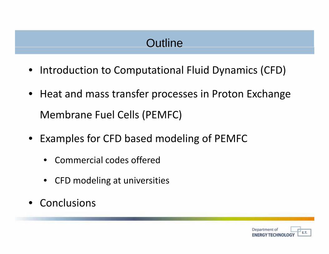
OutlineOut e
• Introduction to Computational Fluid Dynamics (CFD)
• Heat and mass transfer processes in Proton Exchange
M b F l C ll (PEMFC)Membrane Fuel Cells (PEMFC)
• Examples for CFD based modeling of PEMFCp g
• Commercial codes offered
• CFD modeling at universities
• Conclusions
INTRODUCTION TOINTRODUCTION TO COMPUTATIONAL FLUID DYNAMICS
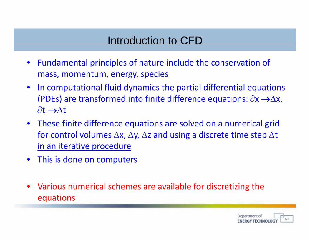
Introduction to CFDt oduct o to C
• Fundamental principles of nature include the conservation of mass momentum energy speciesmass, momentum, energy, species
• In computational fluid dynamics the partial differential equations (PDEs) are transformed into finite difference equations: x x, t t
• These finite difference equations are solved on a numerical grid for control volumes x y z and using a discrete time step tfor control volumes x, y, z and using a discrete time step t in an iterative procedure
• This is done on computers
• Various numerical schemes are available for discretizing the iequations
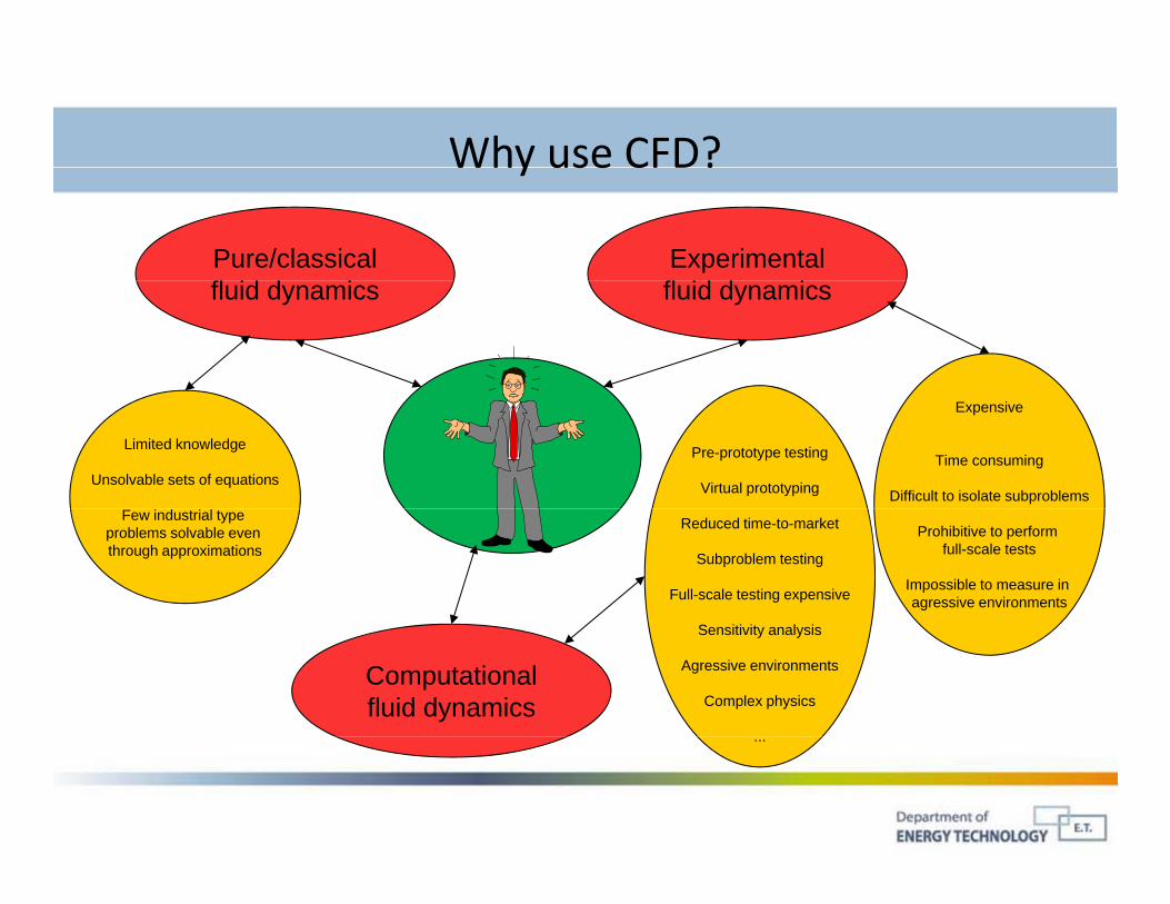
Why use CFD?Why use CFD?
Pure/classicalfl id d i
Experimentalfl id d ifluid dynamics fluid dynamics
Pre-prototype testing
Virtual prototyping
Limited knowledge
Unsolvable sets of equations
Expensive
Time consuming
Difficult to isolate subproblems
Reduced time-to-market
Subproblem testing
Full-scale testing expensive
Few industrial type problems solvable even through approximations
Prohibitive to perform full-scale tests
Impossible to measure in agressive environments
Computationalfluid dynamics
Sensitivity analysis
Agressive environments
Complex physics
...
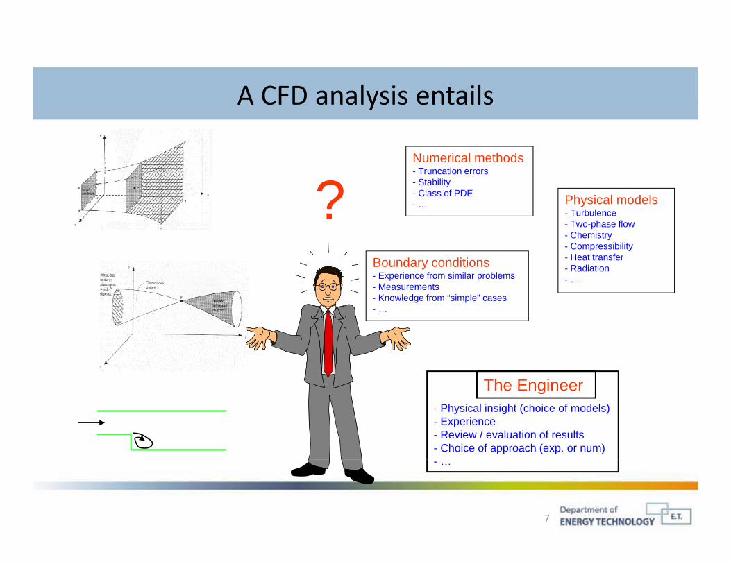
A CFD analysis entailsA CFD analysis entails
Numerical methods- Truncation errors
? - Stability- Class of PDE- … Physical models
- Turbulence- Two-phase flow- Chemistry- Compressibility
Boundary conditions- Experience from similar problems- Measurements- Knowledge from “simple” cases- …
- Compressibility- Heat transfer- Radiation- …
The Engineer- Physical insight (choice of models)- Experience- Review / evaluation of results- Choice of approach (exp. or num)
The Engineer
7
- …
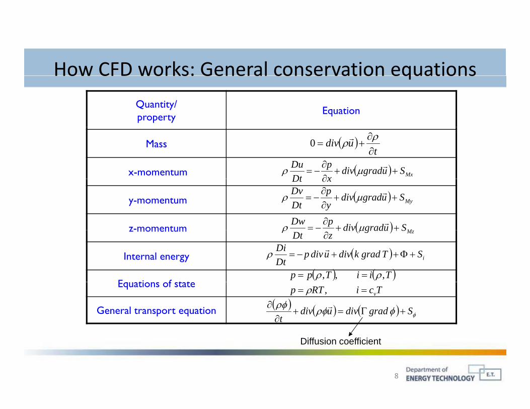
How CFD works: General conservation equationsHow CFD works: General conservation equations
Quantity/property Equation
Mass
x-momentum
t
udiv
0
MxSugraddivxp
DtDu
y-momentum
z-momentum
xDt
MySugraddivyp
DtDv
MSugraddivpDw
z momentum
Internal energy
E ti f t t
MzSugraddivzDt
iSTgradkdivudivpDtDi
TiiTpp ,,, Equations of state
General transport equation
TciRTp v , Sgraddivudiv
t
8
Diffusion coefficient
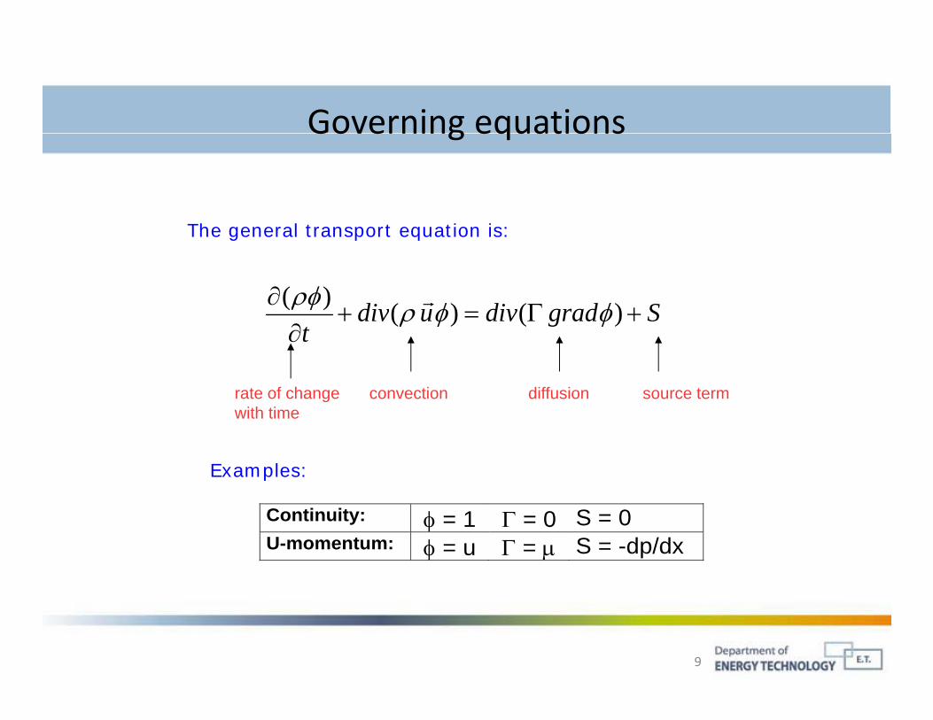
Governing equationsGoverning equations
Th l t t ti iThe general transport equation is:
Sgraddivudiv )()()( Sgraddivudiv
t
)()(
rate of change convection diffusion source termwith time
Examples:
Continuity: = 1 = 0 S = 0 U-momentum: = u = S = -dp/dx
9
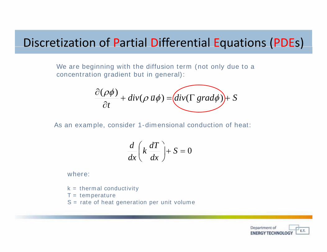
Discretization of Partial Differential Equations (PDEs)Discretization of Partial Differential Equations (PDEs)
We are beginning with the diffusion term (not only due to a concentration gradient but in general):
Sgraddivudivt
)()()(
As an example, consider 1-dimensional conduction of heat:
0
S
dxdTk
dxd
where:where:
k = thermal conductivityT = temperatureS = rate of heat generation per unit volume
Discretization of Partial Differential Equations (PDEs)Discretization of Partial Differential Equations (PDEs)
Consider the 1-dimensional grid system (y and z = 1):
w ewx)( ex)(
W P E
x
We integrate the heat equation over this volume:
0
dxS
dxdTk
dxdTk
e
wwe
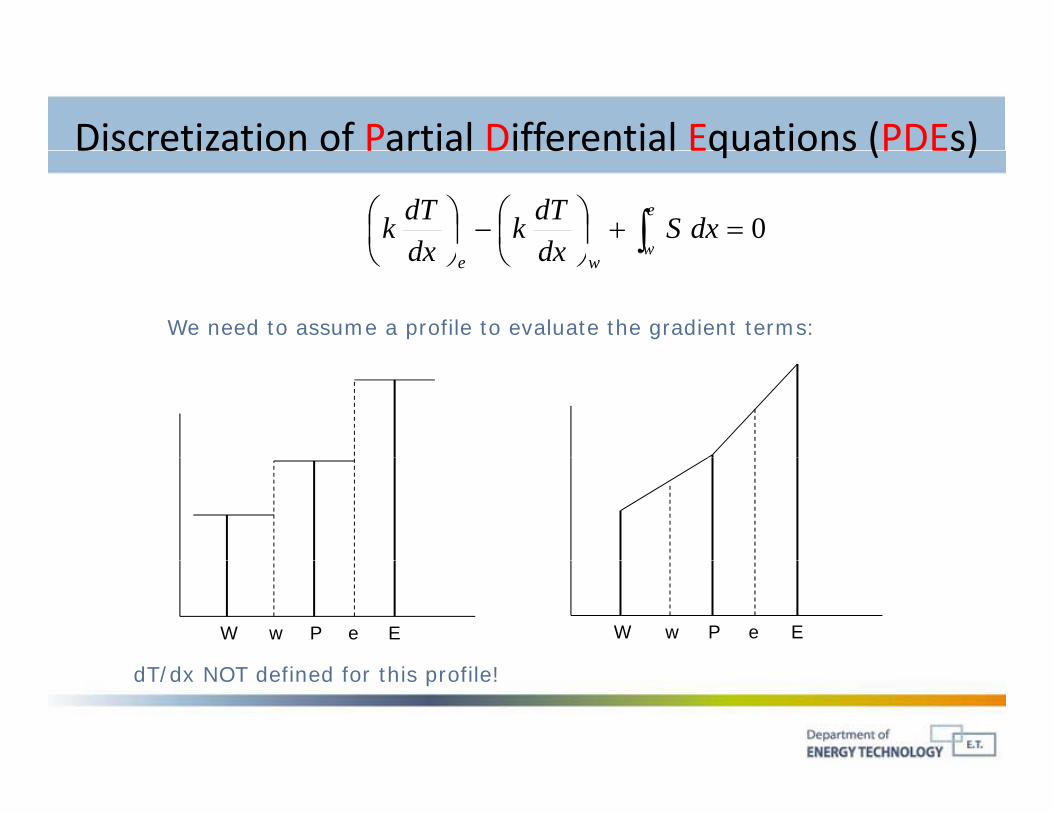
Discretization of Partial Differential Equations (PDEs)
0
dxS
dxdTk
dxdTk
e
w
Discretization of Partial Differential Equations (PDEs)
dxdx wwe
We need to assume a profile to evaluate the gradient terms:
W w P e E W w P e E
dT/dx NOT defined for this profile!
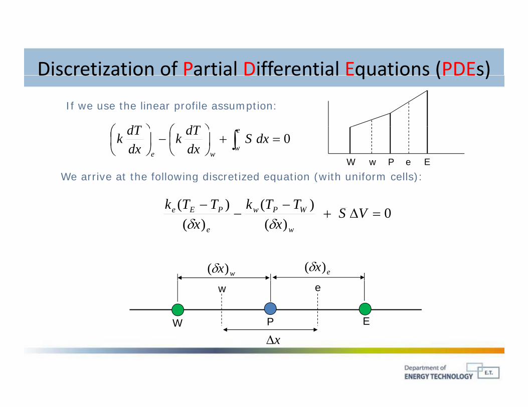
Discretization of Partial Differential Equations (PDEs)
If we use the linear profile assumption:
dTdT
Discretization of Partial Differential Equations (PDEs)
W w P e EWe arrive at the following discretized equation (with uniform cells):
0
dxS
dxdTk
dxdTk
e
wwe
0)(
)()(
)(
VSx
TTkx
TTk
w
WPw
e
PEe
We arrive at the following discretized equation (with uniform cells):
wx)( ex)(
)()( we
W P E
w e
x
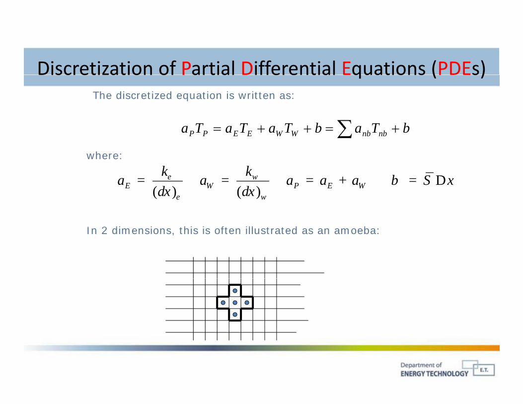
Discretization of Partial Differential Equations (PDEs)The discretized equation is written as:
bTbTTT
Discretization of Partial Differential Equations (PDEs)
bTabTaTaTa nbnbWWEEPP
where:
e wk k b S+ D( ) ( )
e wE W P E W
e w
a a a a a b S xx xd d
= = = + = D
I 2 di i thi i ft ill t t d bIn 2 dimensions, this is often illustrated as an amoeba:
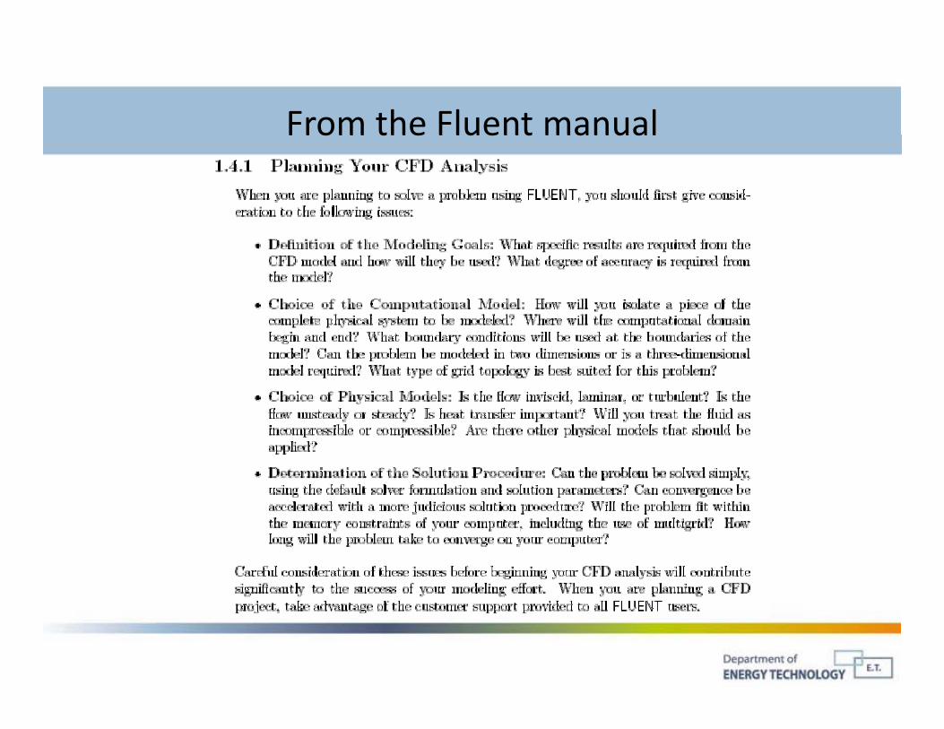
From the Fluent manualFrom the Fluent manual
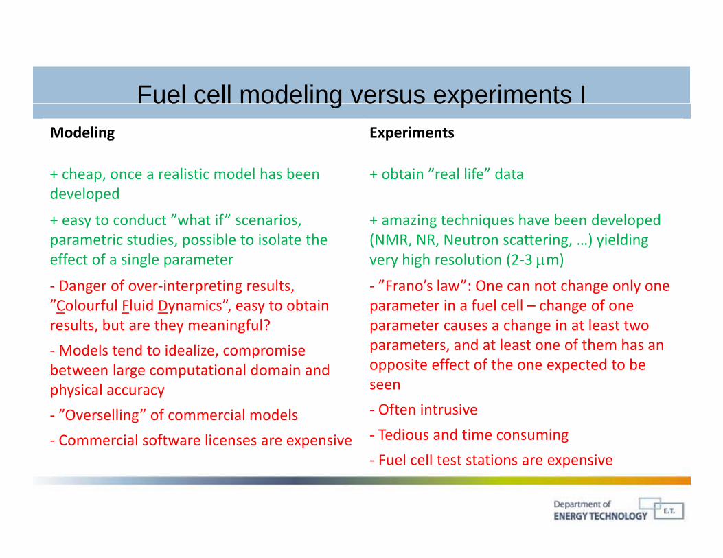
Fuel cell modeling versus experiments Iue ce ode g e sus e pe e tsModeling Experiments
+ cheap once a realistic model has been + obtain ”real life” data+ cheap, once a realistic model has been developed
+ obtain real life data
+ easy to conduct ”what if” scenarios, parametric studies, possible to isolate the
+ amazing techniques have been developed (NMR, NR, Neutron scattering, …) yieldingparametric studies, possible to isolate the
effect of a single parameter(NMR, NR, Neutron scattering, …) yielding very high resolution (2‐3 m)
‐ Danger of over‐interpreting results, ”Colourful Fluid Dynamics”, easy to obtain
‐ ”Frano’s law”: One can not change only one parameter in a fuel cell – change of one
results, but are they meaningful?
‐Models tend to idealize, compromise between large computational domain and h i l
parameter causes a change in at least two parameters, and at least one of them has an opposite effect of the one expected to be seenphysical accuracy
‐ ”Overselling” of commercial models
‐ Commercial software licenses are expensive
seen
‐ Often intrusive
‐ Tedious and time consuming
F l ll i i‐ Fuel cell test stations are expensive
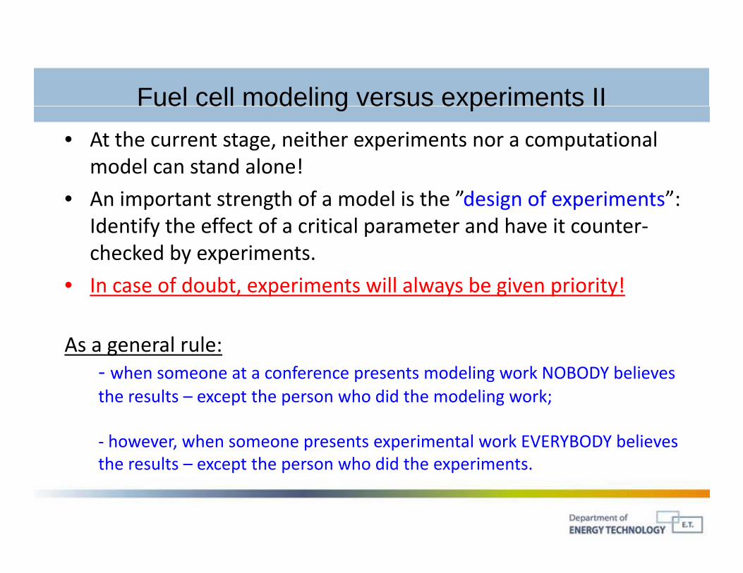
Fuel cell modeling versus experiments IIue ce ode g e sus e pe e ts• At the current stage, neither experiments nor a computational
model can stand alone!
• An important strength of a model is the ”design of experiments”: Identify the effect of a critical parameter and have it counter‐checked by experimentschecked by experiments.
• In case of doubt, experiments will always be given priority!
As a general rule:‐ when someone at a conference presents modeling work NOBODY believes the results except the person who did the modeling work;the results – except the person who did the modeling work;
‐ however, when someone presents experimental work EVERYBODY believes the results – except the person who did the experimentsthe results except the person who did the experiments.
HEAT AND MASS TRANSFER INHEAT AND MASS TRANSFER IN PROTON EXCHANGE MEMBRANE FUEL CELLS (PEMFC)FUEL CELLS (PEMFC)
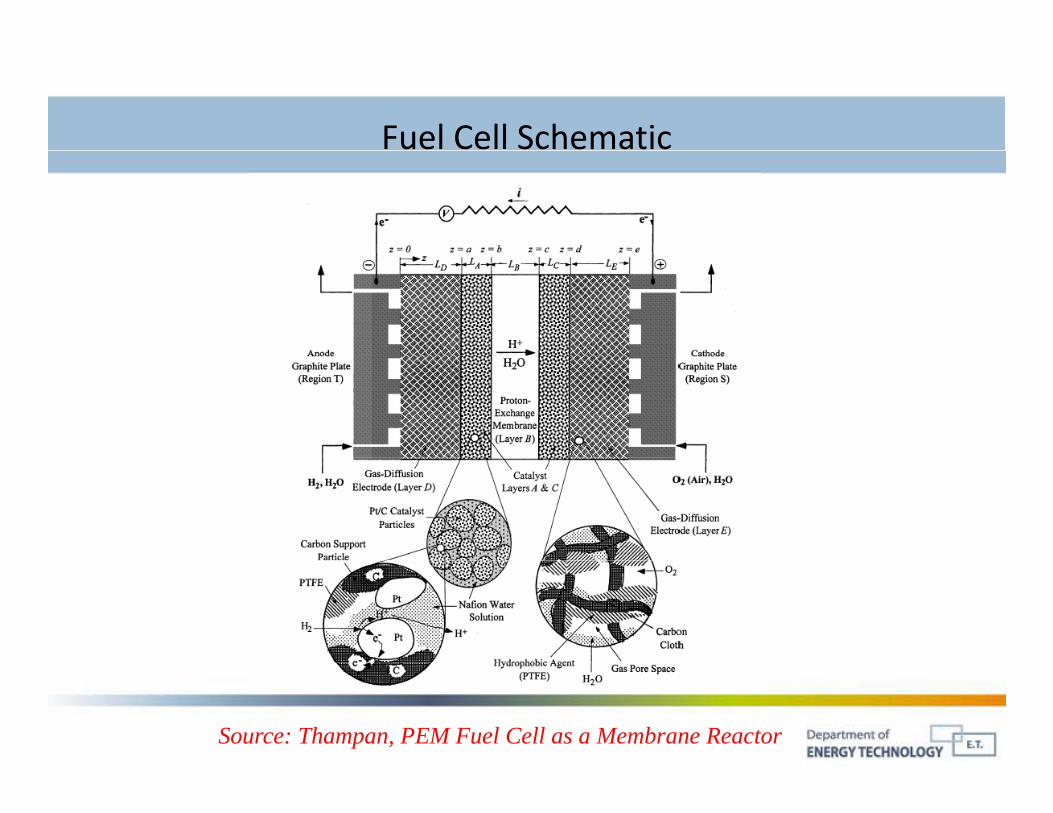
Fuel Cell Schematic
Source: Thampan, PEM Fuel Cell as a Membrane Reactor
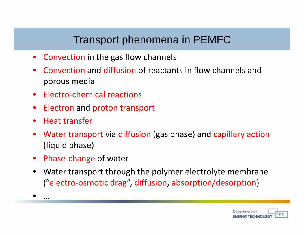
Transport phenomena in PEMFCa spo t p e o e a C• Convection in the gas flow channels
• Convection and diffusion of reactants in flow channels andConvection and diffusion of reactants in flow channels and porous media
• Electro‐chemical reactions
• Electron and proton transport
• Heat transfer
W t t t i diff i ( h ) d ill ti• Water transport via diffusion (gas phase) and capillary action (liquid phase)
• Phase‐change of waterg
• Water transport through the polymer electrolyte membrane (”electro‐osmotic drag”, diffusion, absorption/desorption)
• …
CFD modeling of PEMFCC ode g o C
• Due to the plethora of transport phenomena, CFD is a very good approach to try and cover all (or most) of these physics.
• Commercial CFD codes (e.g. Fluent, Star‐CD, CFX 13, CFD ACE) offer tools to solve time dependent transport equations for mass, momentum, species, and energy, and can be modified in order to model heat and mass transfer in fuel cells.model heat and mass transfer in fuel cells.
• For complex geometries, one or two‐dimensional models are not sufficient to investigate all these phenomena (but are suitable to picksufficient to investigate all these phenomena (but are suitable to pick a few aspects and study those in greater detail using analytical modeling)…
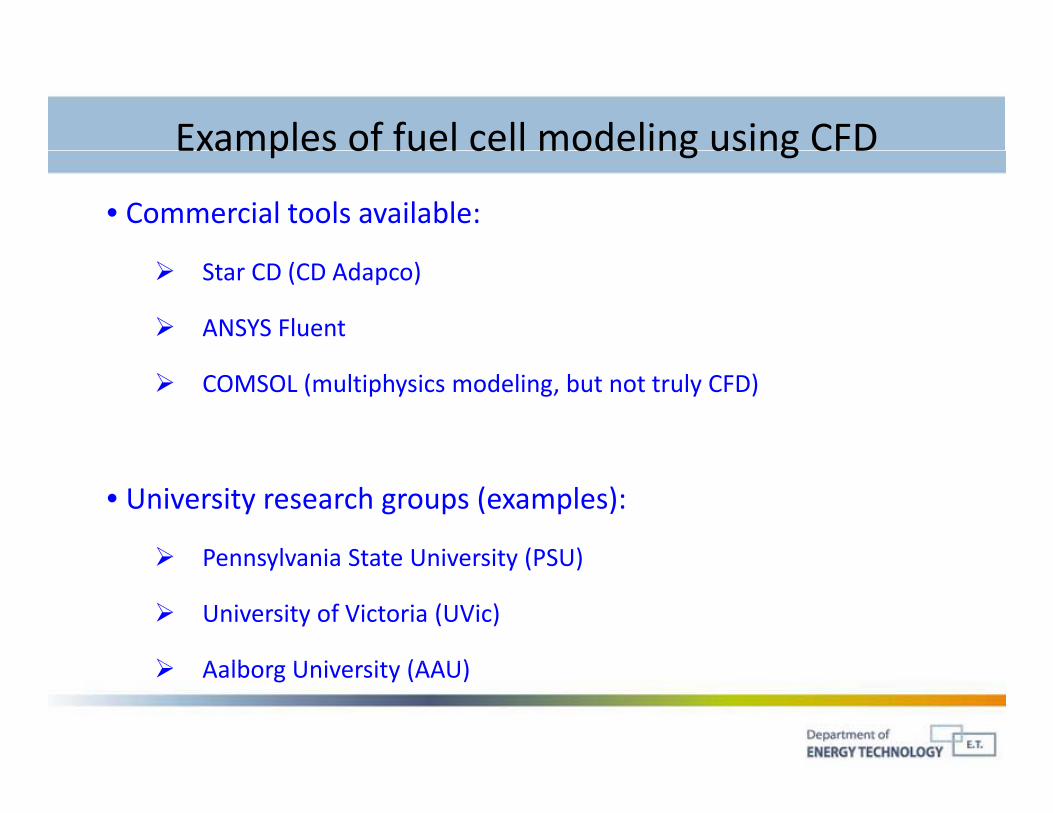
Examples of fuel cell modeling using CFDExamples of fuel cell modeling using CFD
• Commercial tools available:
Star CD (CD Adapco)
ANSYS Fluent
COMSOL (multiphysics modeling, but not truly CFD)
• University research groups (examples):
Pennsylvania State University (PSU) Pennsylvania State University (PSU)
University of Victoria (UVic)
A lb U i it (AAU) Aalborg University (AAU)
COMMERCIAL FUEL CELL MODELSCOMMERCIAL FUEL CELL MODELS EMPLOYING CFD
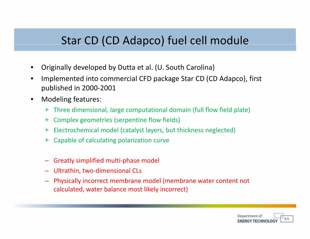
Star CD (CD Adapco) fuel cell moduleStar CD (CD Adapco) fuel cell module
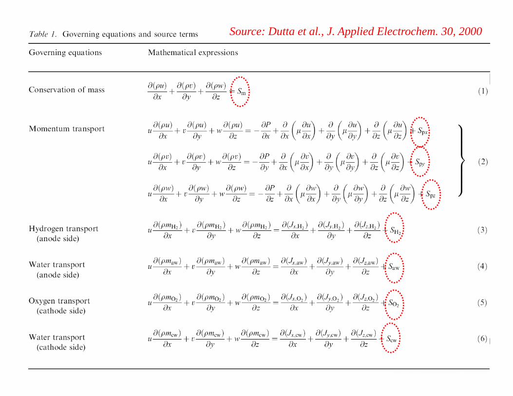
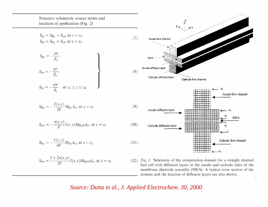
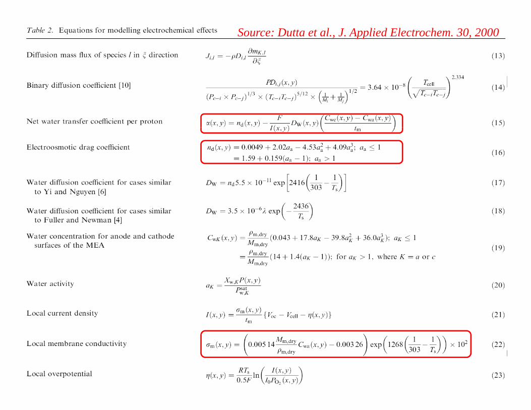
• Originally developed by Dutta et al. (U. South Carolina)
• Implemented into commercial CFD package Star CD (CD Adapco), first published in 2000‐2001
• Modeling features:+ Three dimensional, large computational domain (full flow field plate)
+ Complex geometries (serpentine flow fields)
+ Electrochemical model (catalyst layers, but thickness neglected)
+ Capable of calculating polarization curve
– Greatly simplified multi‐phase model
– Ultrathin, two‐dimensional CLs
– Physically incorrect membrane model (membrane water content not calculated, water balance most likely incorrect)
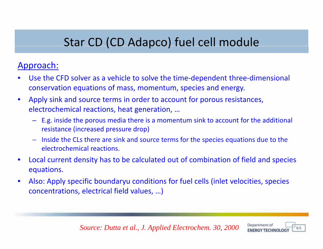
Star CD (CD Adapco) fuel cell moduleStar CD (CD Adapco) fuel cell module
Approach:• Use the CFD solver as a vehicle to solve the time dependent three dimensional• Use the CFD solver as a vehicle to solve the time‐dependent three‐dimensional
conservation equations of mass, momentum, species and energy.
• Apply sink and source terms in order to account for porous resistances, electrochemical reactions heat generationelectrochemical reactions, heat generation, …– E.g. inside the porous media there is a momentum sink to account for the additional
resistance (increased pressure drop)
– Inside the CLs there are sink and source terms for the species equations due to theInside the CLs there are sink and source terms for the species equations due to the electrochemical reactions.
• Local current density has to be calculated out of combination of field and species equations.equations.
• Also: Apply specific boundaryu conditions for fuel cells (inlet velocities, species concentrations, electrical field values, …)
Source: Dutta et al., J. Applied Electrochem. 30, 2000
Source: Dutta et al., J. Applied Electrochem. 30, 2000
Source: Dutta et al., J. Applied Electrochem. 30, 2000
Source: Dutta et al., J. Applied Electrochem. 30, 2000
A critical note on commercial CFD modulesA critical note on commercial CFD modules
• It can be seen from the previous equations that altogether there are as many unknowns as there are equations:are as many unknowns as there are equations:– Continuity equations and the coupling with three momentum equations
yield p, u, v, w.
Energy equation: T– Energy equation: T.
– Electrical field equation: .– Butler‐Volmer equation, Nernst Planck equation: electrical overpotential
l l t d it i, local current density i.
• Hence it is ensured that there is a solvable system of equations
• The need for user convenience ensures that the user will get asolution to this system of equations, but it must be asked, whether all the physical equations and the model is correct!
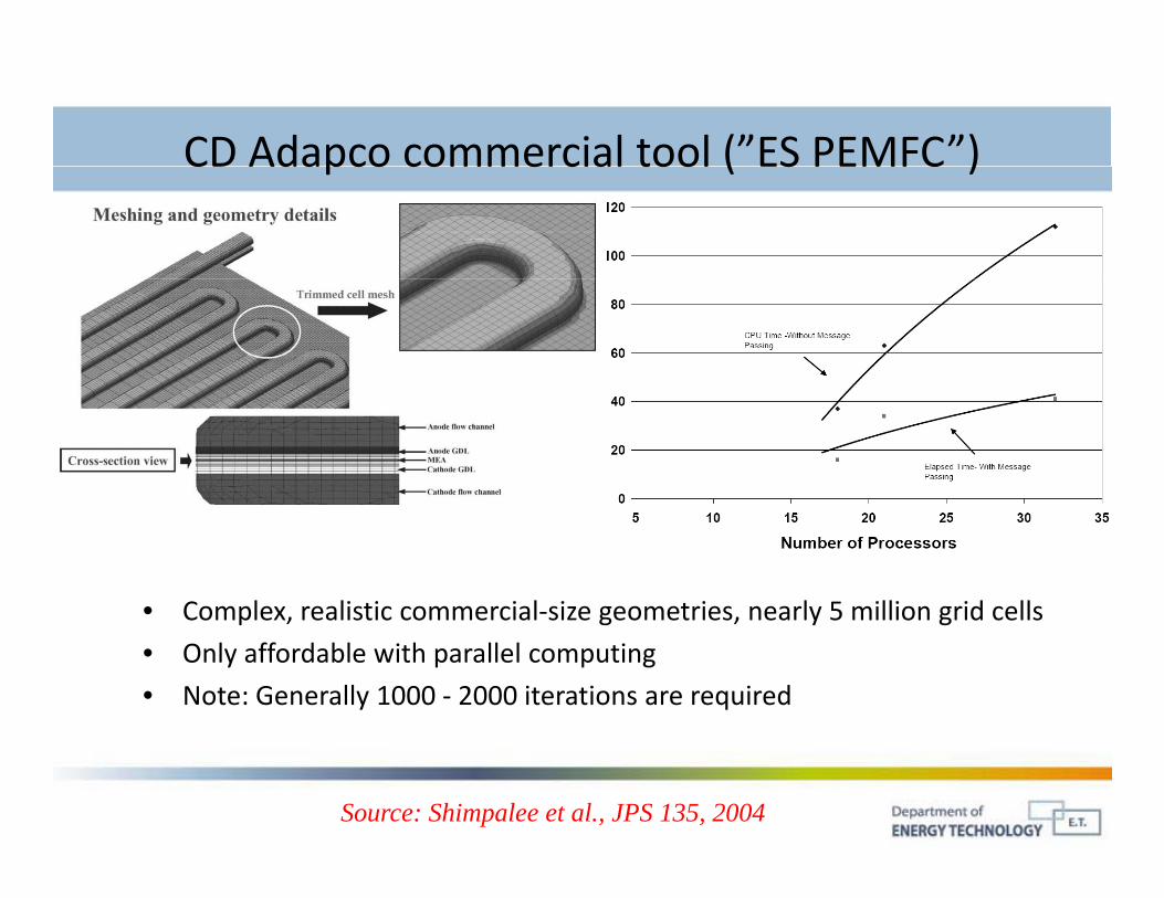
CD Adapco commercial tool (”ES PEMFC”)CD Adapco commercial tool ( ES PEMFC )
• Complex, realistic commercial‐size geometries, nearly 5 million grid cellsComplex, realistic commercial size geometries, nearly 5 million grid cells
• Only affordable with parallel computing
• Note: Generally 1000 ‐ 2000 iterations are required
Source: Shimpalee et al., JPS 135, 2004
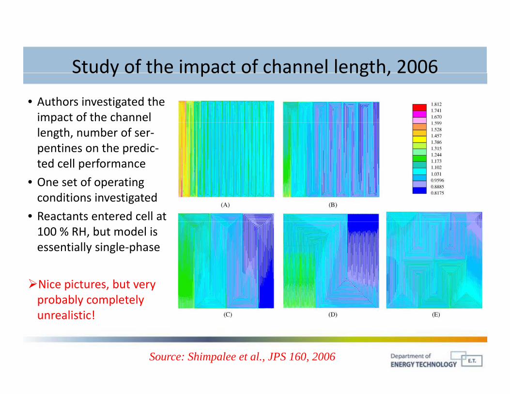
Study of the impact of channel length, 2006Study of the impact of channel length, 2006
• Authors investigated the impact of the channel plength, number of ser‐pentines on the predic‐ted cell performance
• One set of operating conditions investigated
• Reactants entered cell at 100 % RH, but model is essentially single‐phase
Nice pictures, but very probably completely unrealistic!
Source: Shimpalee et al., JPS 160, 2006
Summary: Commercial module es‐pemfc (CD Adapco)Summary: Commercial module es pemfc (CD Adapco)• First commercial tool, state‐of‐the‐art in 2000.
• In general, many of the physics are encountered and highly complex, g y p y g y pcommercial size geometries can be calculated (on parallel computers one case can take up to 50h).
• Trade‐off between physical accuracy (membrane model, multi‐phase flow) p y y pversus the need of obtaining a result.
• Since development of that model, advances have been made in the understanding of multi‐phase flow issues in porous media and channels, not yet accounted for in this model.
• On balance, this model was the first commercial tool and state‐of‐the‐art in 2000, but it has not been further developed to a sufficient degree.
• Results are questionable, but polarization curves can be easily measured (validation possible).
• It is not recommended to use this model for PhD research!It is not recommended to use this model for PhD research!
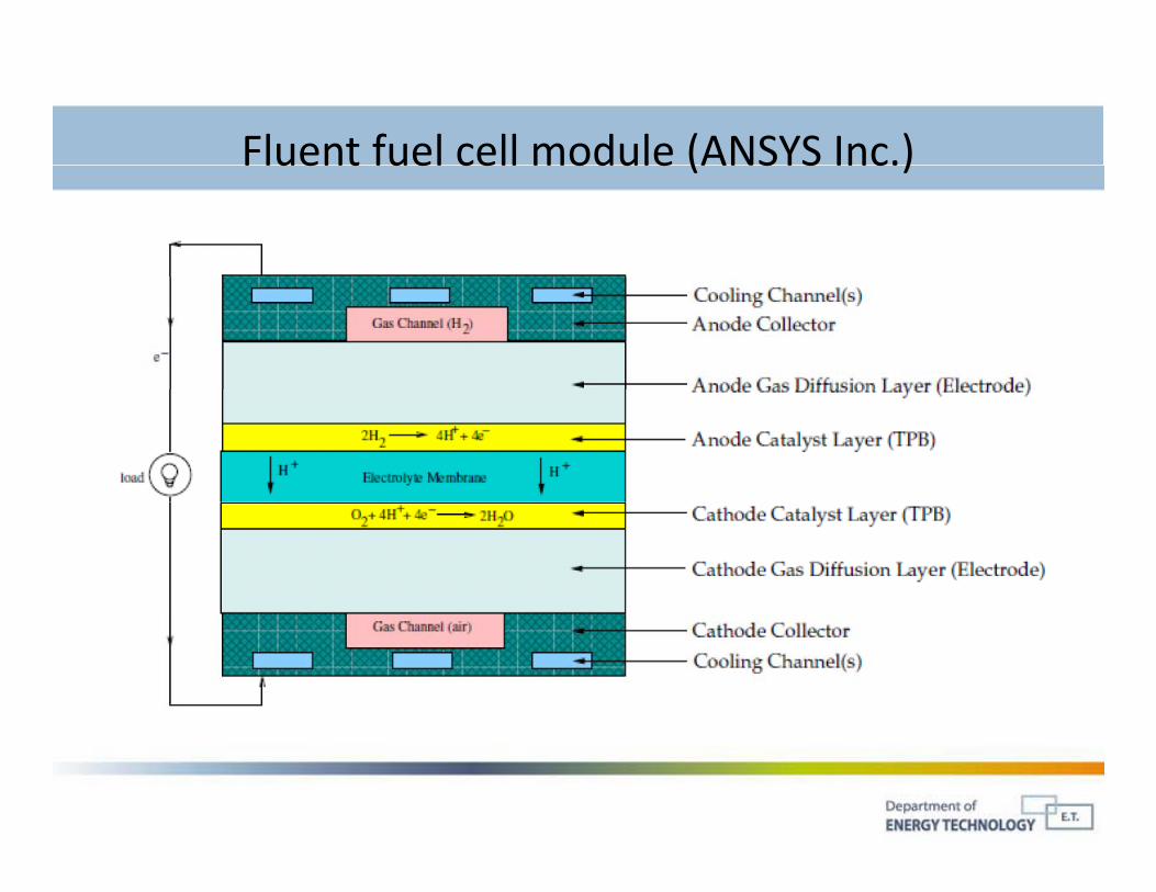
Fluent fuel cell module (ANSYS Inc.)Fluent fuel cell module (ANSYS Inc.)
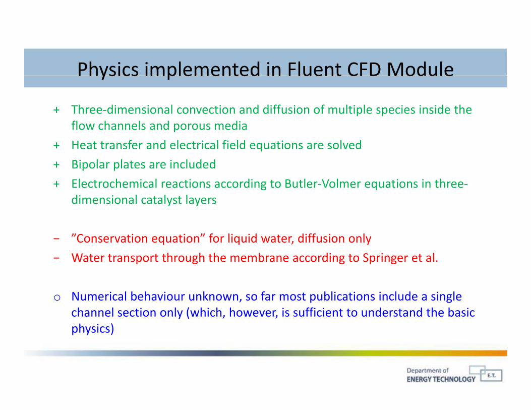
Physics implemented in Fluent CFD ModulePhysics implemented in Fluent CFD Module
+ Three‐dimensional convection and diffusion of multiple species inside the flow channels and porous mediaflow channels and porous media
+ Heat transfer and electrical field equations are solved
+ Bipolar plates are included
l h i l i di l V l i i h+ Electrochemical reactions according to Butler‐Volmer equations in three‐dimensional catalyst layers
− ”Conservation equation” for liquid water, diffusion only
− Water transport through the membrane according to Springer et al.
o Numerical behaviour unknown, so far most publications include a single channel section only (which, however, is sufficient to understand the basic physics)p y )
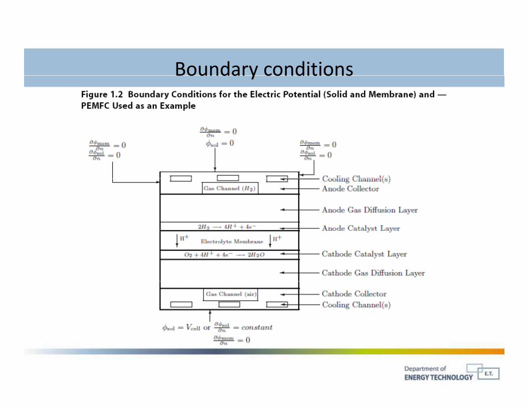
Boundary conditionsBoundary conditions
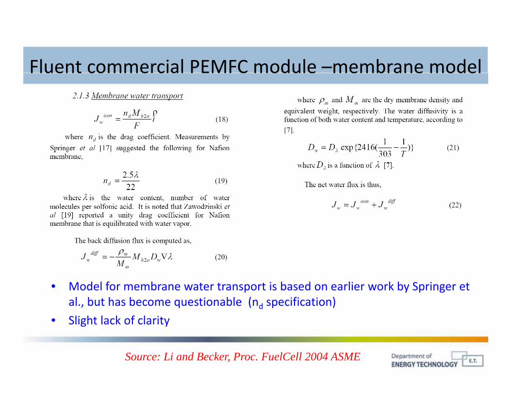
Fluent commercial PEMFC module –membrane modelFluent commercial PEMFC module membrane model
• Model for membrane water transport is based on earlier work by Springer et al., but has become questionable (nd specification)
• Slight lack of clarity• Slight lack of clarity
Source: Li and Becker, Proc. FuelCell 2004 ASME
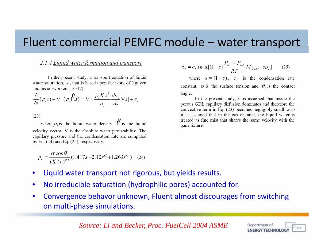
Fluent commercial PEMFC module – water transportFluent commercial PEMFC module water transport
• Liquid water transport not rigorous but yields results• Liquid water transport not rigorous, but yields results.
• No irreducible saturation (hydrophilic pores) accounted for.
• Convergence behavor unknown, Fluent almost discourages from switching l h lon multi‐phase simulations.
Source: Li and Becker, Proc. FuelCell 2004 ASME
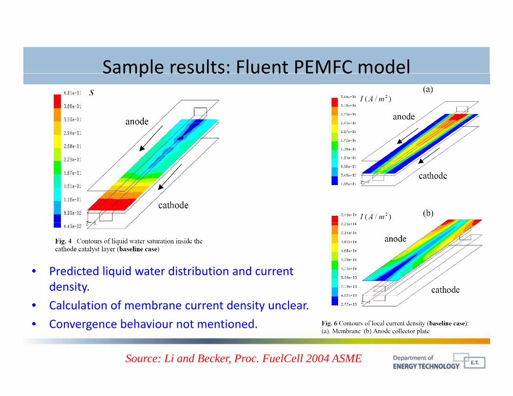
Sample results: Fluent PEMFC modelSample results: Fluent PEMFC model
• Predicted liquid water distribution and currentPredicted liquid water distribution and current density.
• Calculation of membrane current density unclear.
• Convergence behaviour not mentioned• Convergence behaviour not mentioned.
Source: Li and Becker, Proc. FuelCell 2004 ASME
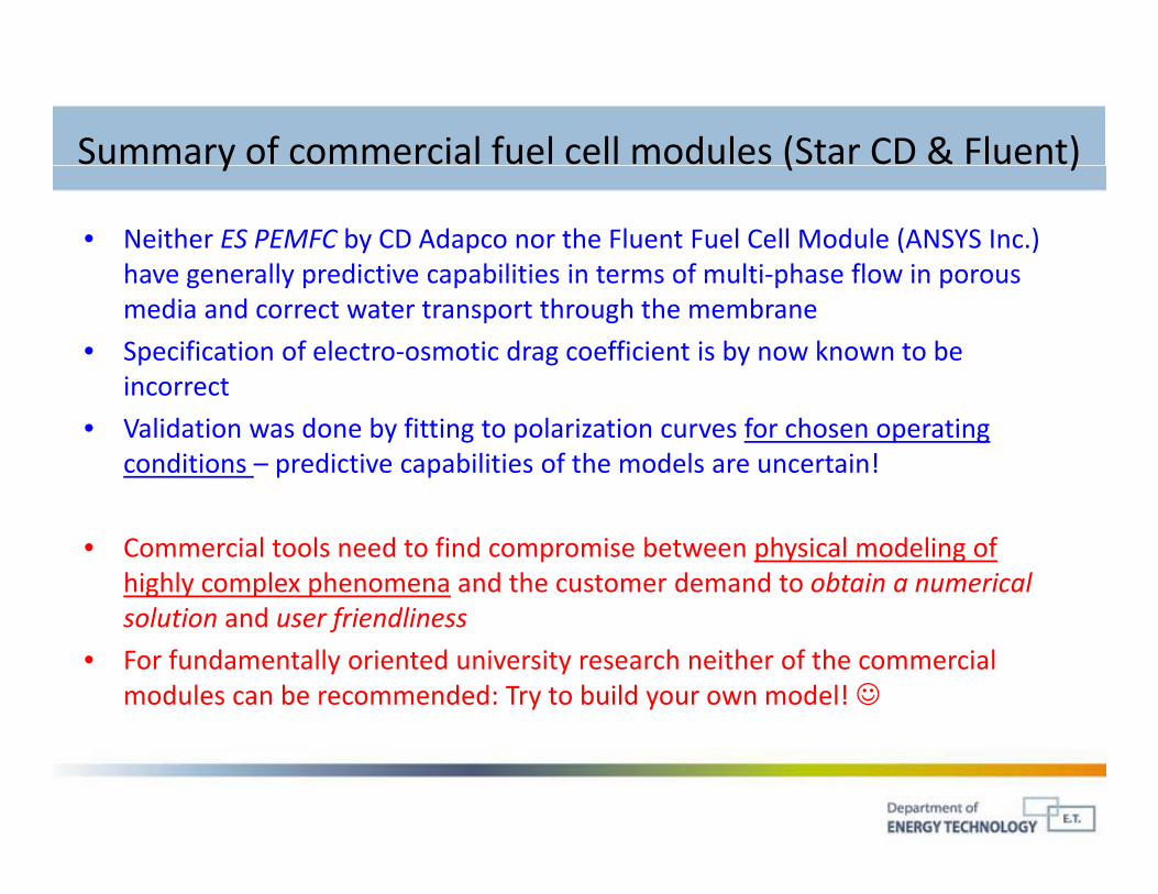
Summary of commercial fuel cell modules (Star CD & Fluent)y ( )
• Neither ES PEMFC by CD Adapco nor the Fluent Fuel Cell Module (ANSYS Inc.) have generally predictive capabilities in terms of multi‐phase flow in poroushave generally predictive capabilities in terms of multi phase flow in porous media and correct water transport through the membrane
• Specification of electro‐osmotic drag coefficient is by now known to be incorrectincorrect
• Validation was done by fitting to polarization curves for chosen operating conditions – predictive capabilities of the models are uncertain!
• Commercial tools need to find compromise between physical modeling of highly complex phenomena and the customer demand to obtain a numerical solution and user friendlinesssolution and user friendliness
• For fundamentally oriented university research neither of the commercial modules can be recommended: Try to build your own model!

UNIVERSITY FUEL CELL MODELSUNIVERSITY FUEL CELL MODELS EMPLOYING CFD
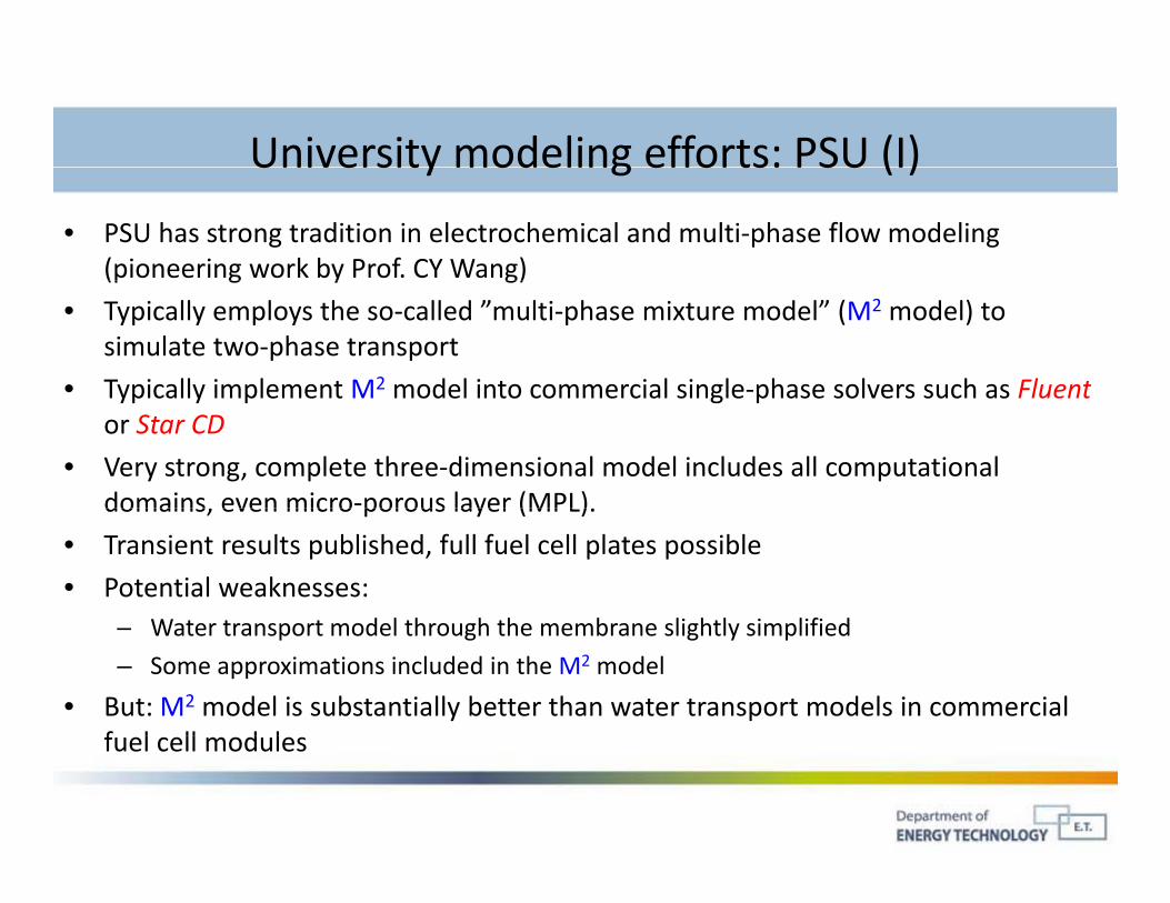
University modeling efforts: PSU (I)University modeling efforts: PSU (I)
• PSU has strong tradition in electrochemical and multi‐phase flow modeling (pioneering work by Prof. CY Wang)(p g y g)
• Typically employs the so‐called ”multi‐phase mixture model” (M2 model) to simulate two‐phase transport
• Typically implement M2 model into commercial single‐phase solvers such as FluentTypically implement M model into commercial single phase solvers such as Fluentor Star CD
• Very strong, complete three‐dimensional model includes all computational domains, even micro‐porous layer (MPL).domains, even micro porous layer (MPL).
• Transient results published, full fuel cell plates possible
• Potential weaknesses: W t t t d l th h th b li htl i lifi d– Water transport model through the membrane slightly simplified
– Some approximations included in the M2 model
• But: M2 model is substantially better than water transport models in commercial f l ll d lfuel cell modules
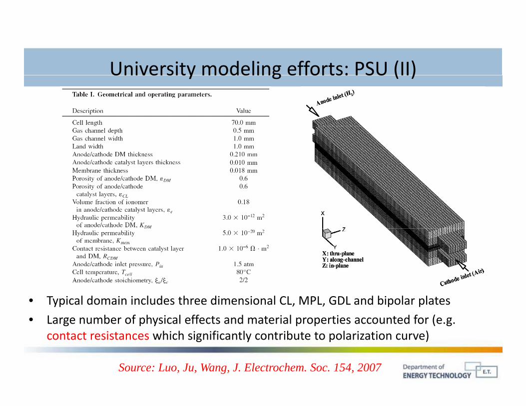
University modeling efforts: PSU (II)University modeling efforts: PSU (II)
• Typical domain includes three dimensional CL, MPL, GDL and bipolar plates
• Large number of physical effects and material properties accounted for (e.g. i hi h i ifi l ib l i i )contact resistances which significantly contribute to polarization curve)
Source: Luo, Ju, Wang, J. Electrochem. Soc. 154, 2007
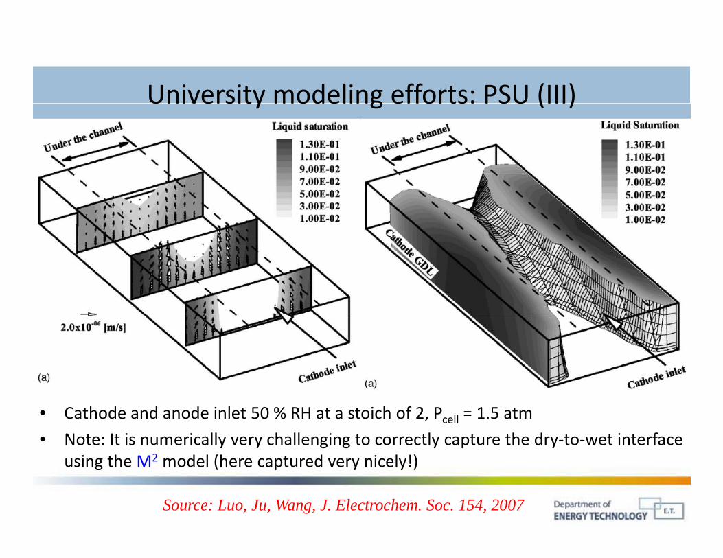
University modeling efforts: PSU (III)University modeling efforts: PSU (III)
• Cathode and anode inlet 50 % RH at a stoich of 2, Pcell = 1.5 atm
• Note: It is numerically very challenging to correctly capture the dry‐to‐wet interface i h 2 d l (h d i l !)using the M2 model (here captured very nicely!)
Source: Luo, Ju, Wang, J. Electrochem. Soc. 154, 2007
University modeling efforts: AAUUniversity modeling efforts: AAU
• Among the few groups that employ the multi‐fluid approach to simulate multi‐phase flow (other groups: Gurau et al.)p ( g p )
• Use formerly commercial software CFX‐4 (AEA Technology, later ANSYS Inc.)– Initial work by M. Bang at AAU
– Later on combination with Berning and Djilali (UVic), also utilizing publication byLater on combination with Berning and Djilali (UVic), also utilizing publication by Gurau et al.
• Salient features of CFX‐4Salient features of CFX 4 – Currently appears to be the only model that utilizes multi‐fluid approach to simulate
two‐phase flow (stand alone feature)
– No parallel code, only small computational domains possible (one ”repeat unit”)No parallel code, only small computational domains possible (one repeat unit )
– Structured grid: only simple geometries are possible (but this is no disadvantage for PEFC)
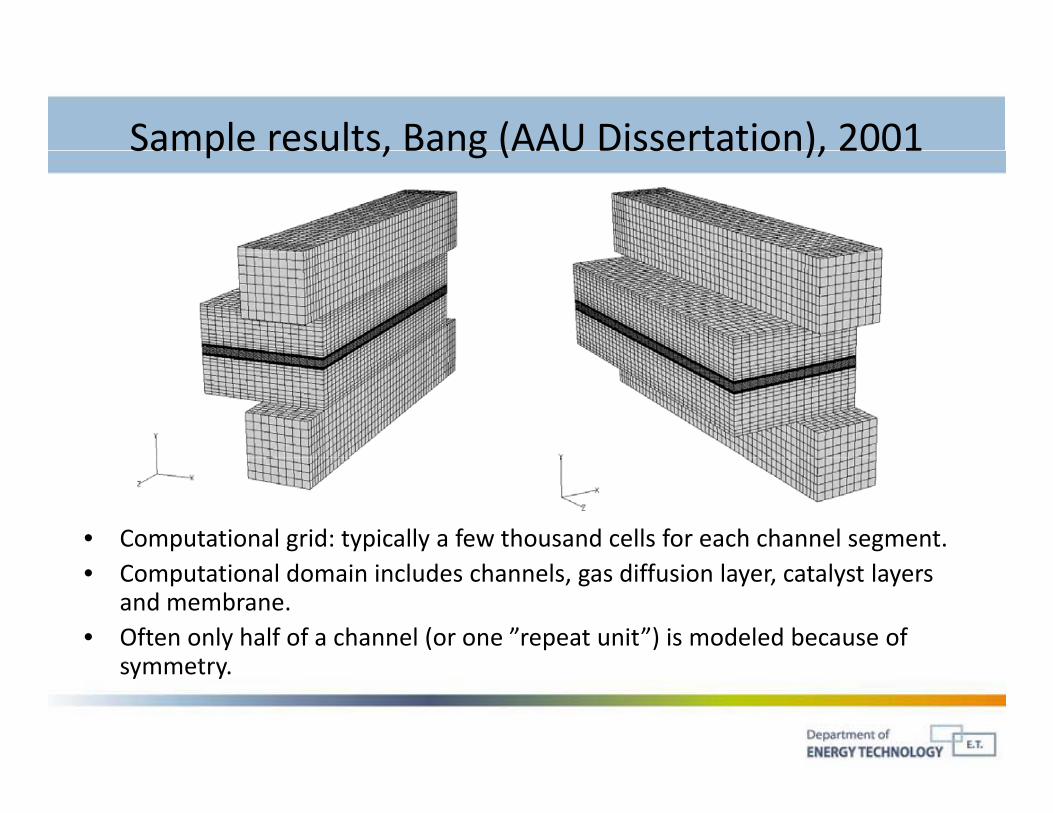
Sample results, Bang (AAU Dissertation), 2001Sample results, Bang (AAU Dissertation), 2001
• Computational grid: typically a few thousand cells for each channel segment.• Computational domain includes channels, gas diffusion layer, catalyst layers
and membrane.• Often only half of a channel (or one ”repeat unit”) is modeled because of
symmetrysymmetry.
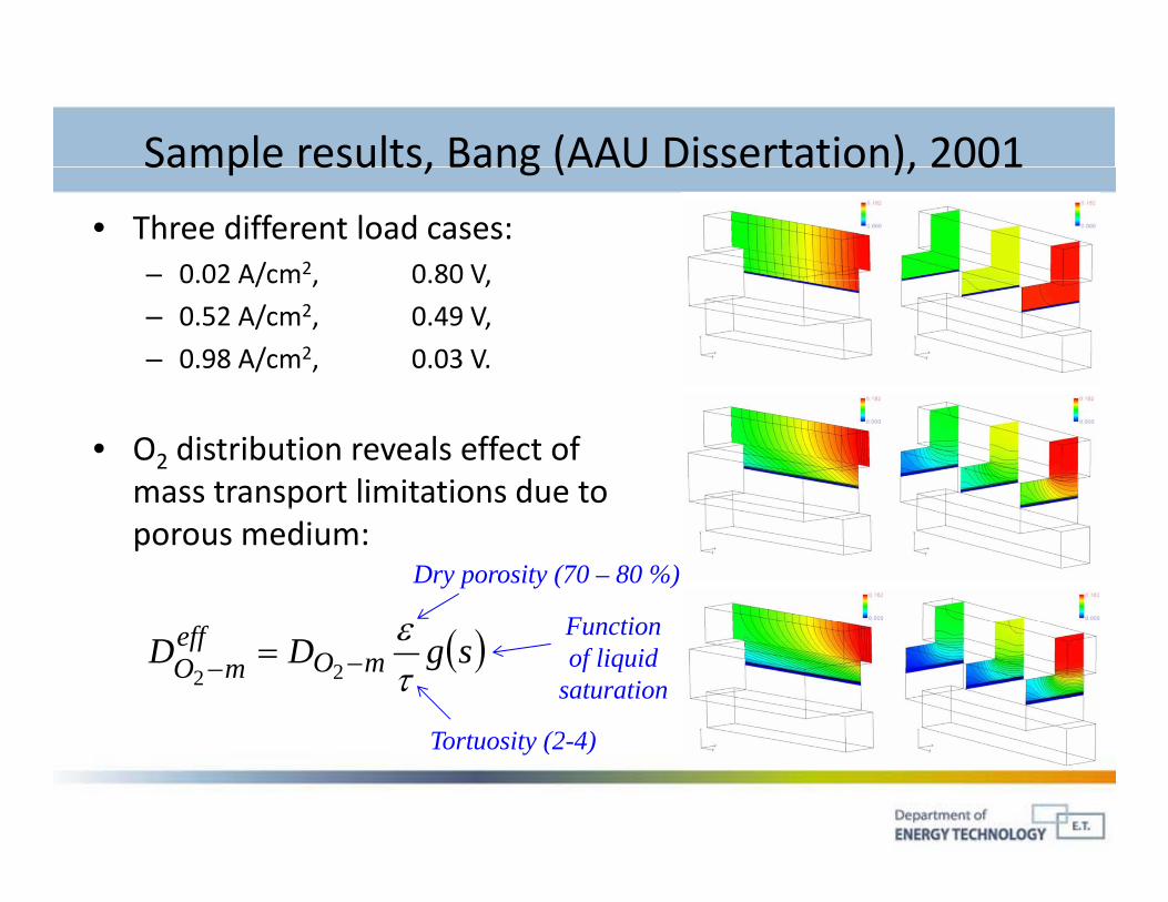
Sample results, Bang (AAU Dissertation), 2001Sample results, Bang (AAU Dissertation), 2001
• Three different load cases:– 0.02 A/cm2, 0.80 V,0.02 A/cm , 0.80 V,
– 0.52 A/cm2, 0.49 V,
– 0.98 A/cm2, 0.03 V.
• O2 distribution reveals effect of mass transport limitations due to pporous medium:
Dry porosity (70 – 80 %)
F ti sgDD mOeff
mO
22
T t it (2 4)
Function of liquid
saturation
Tortuosity (2-4)
Sample results, Bang (AAU Dissertation), 2001Sample results, Bang (AAU Dissertation), 2001
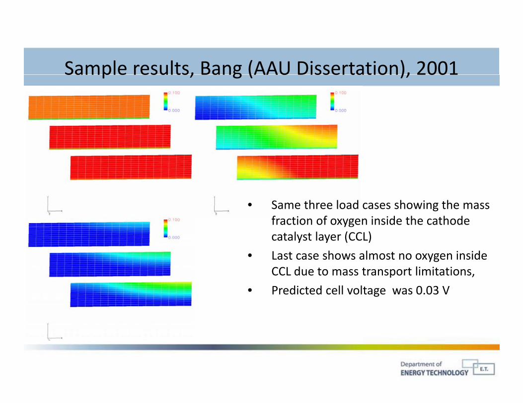
• Same three load cases showing the mass fraction of oxygen inside the cathode ygcatalyst layer (CCL)
• Last case shows almost no oxygen inside CCL due to mass transport limitations,
• Predicted cell voltage was 0.03 V
Sample results, Bang (AAU Dissertation), 2001Sample results, Bang (AAU Dissertation), 2001
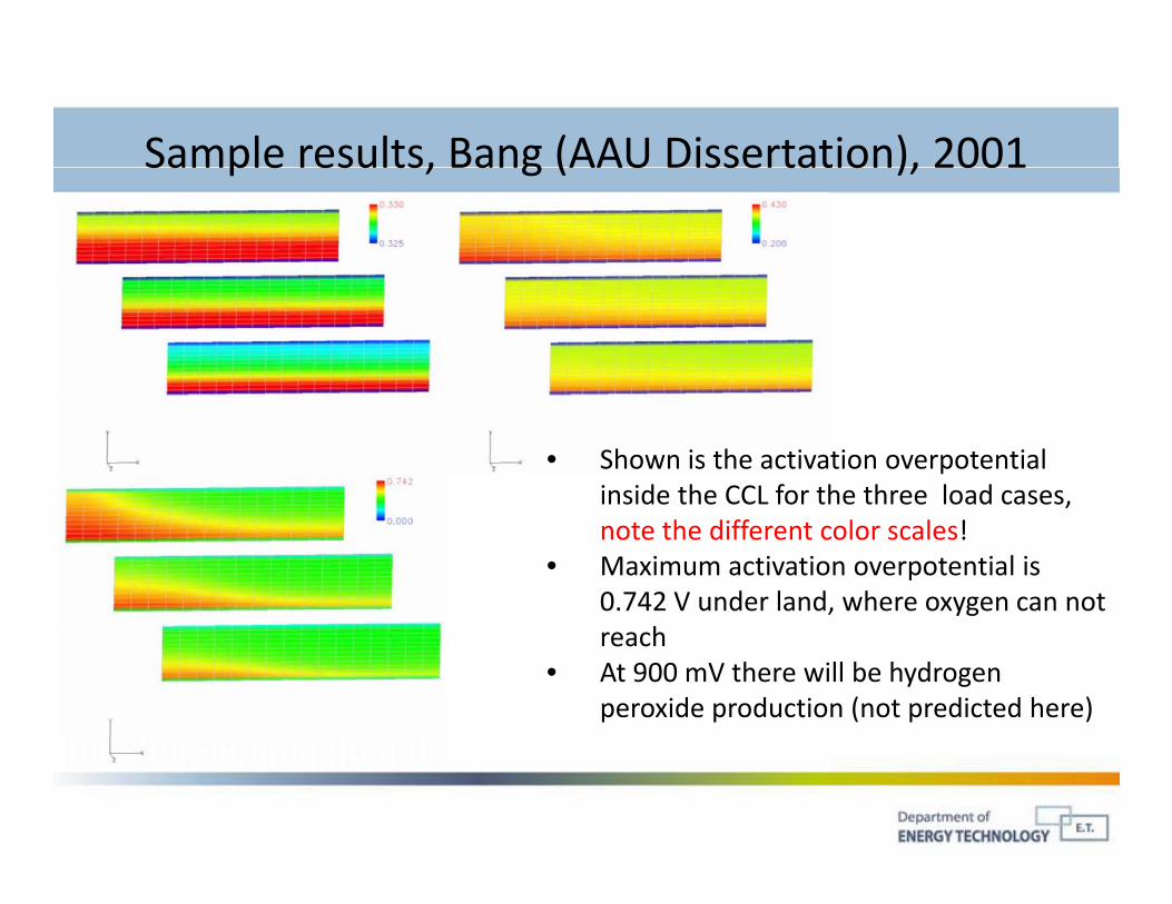
• Shown is the activation overpotential inside the CCL for the three load cases, note the different color scales!
• Maximum activation overpotential is 0.742 V under land, where oxygen can not reach
• At 900 mV there will be hydrogen peroxide production (not predicted here)
Sample results, Bang (AAU Dissertation), 2001Sample results, Bang (AAU Dissertation), 2001
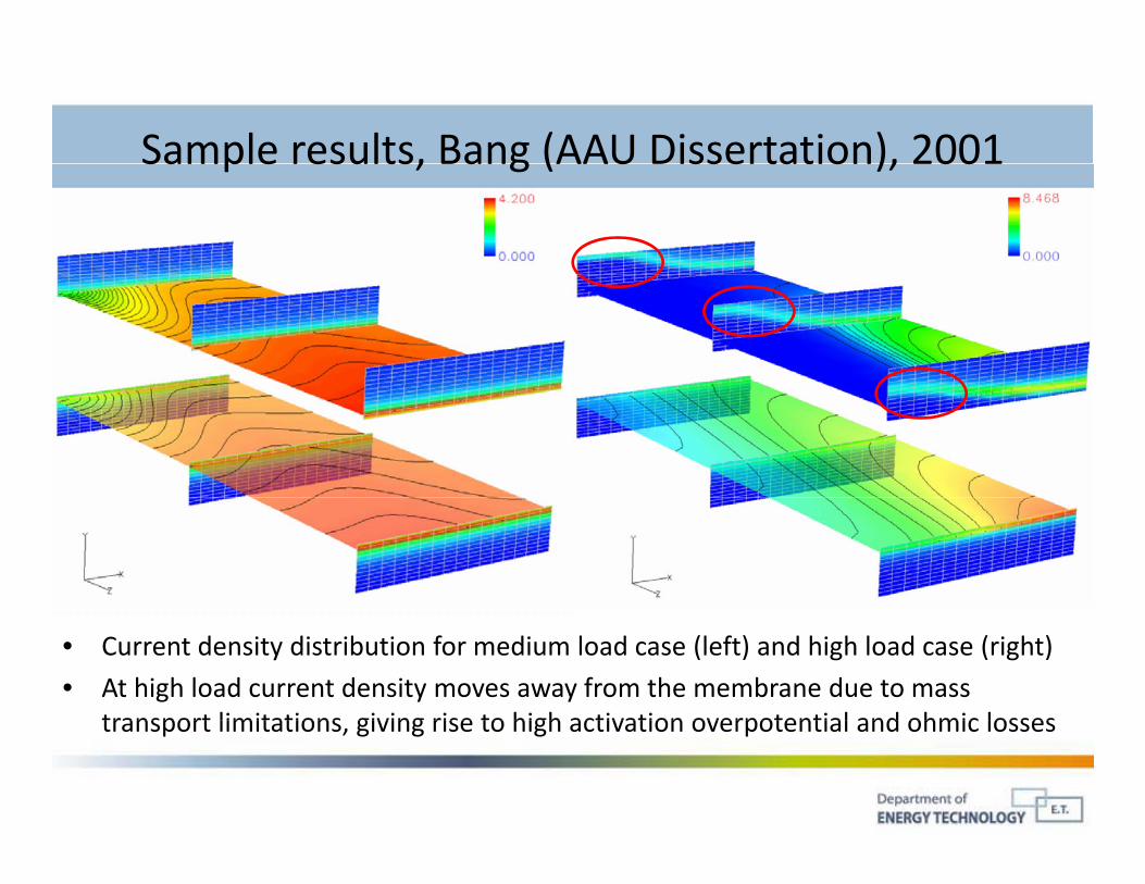
• Current density distribution for medium load case (left) and high load case (right)
• At high load current density moves away from the membrane due to mass transport limitations giving rise to high activation overpotential and ohmic lossestransport limitations, giving rise to high activation overpotential and ohmic losses
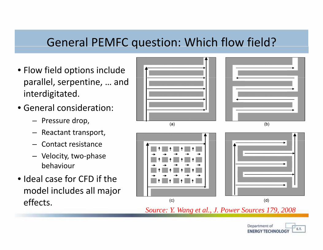
General PEMFC question: Which flow field?General PEMFC question: Which flow field?
• Flow field options include parallel, serpentine, … and interdigitated.
• General consideration:General consideration: – Pressure drop,
– Reactant transport,
– Contact resistance
– Velocity, two‐phase behaviour
• Ideal case for CFD if the model includes all major effectseffects.
Source: Y. Wang et al., J. Power Sources 179, 2008
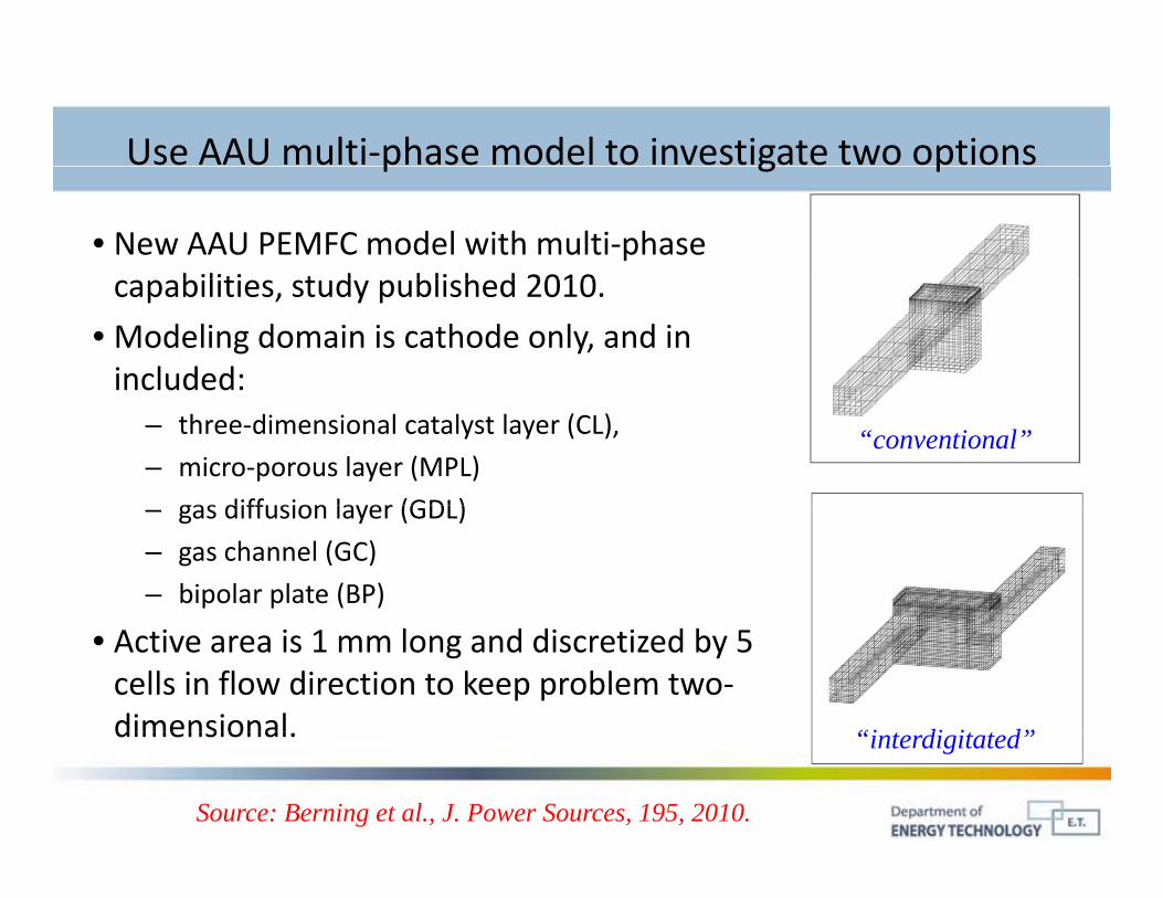
Use AAU multi‐phase model to investigate two options
• New AAU PEMFC model with multi‐phase biliti t d bli h d 2010
p g p
capabilities, study published 2010.
• Modeling domain is cathode only, and in included:
– three‐dimensional catalyst layer (CL),
– micro‐porous layer (MPL)
gas diffusion layer (GDL)
“conventional”
– gas diffusion layer (GDL)
– gas channel (GC)
– bipolar plate (BP)
• Active area is 1 mm long and discretized by 5 cells in flow direction to keep problem two‐dimensional “i di i d”dimensional. “interdigitated”
Source: Berning et al., J. Power Sources, 195, 2010.
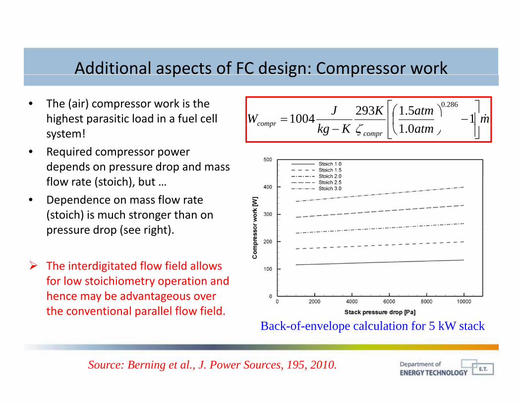
Additional aspects of FC design: Compressor work
• The (air) compressor work is the highest parasitic load in a fuel cell matmK
KkJWcompr
1
015.12931004
286.0
p g p
system!
• Required compressor power depends on pressure drop and mass
atmKkg comprcompr
0.1
flow rate (stoich), but …
• Dependence on mass flow rate (stoich) is much stronger than on
d ( i ht)pressure drop (see right).
The interdigitated flow field allows f l t i hi t ti dfor low stoichiometry operation and hence may be advantageous over the conventional parallel flow field.
Back-of-envelope calculation for 5 kW stackBack of envelope calculation for 5 kW stack
Source: Berning et al., J. Power Sources, 195, 2010.
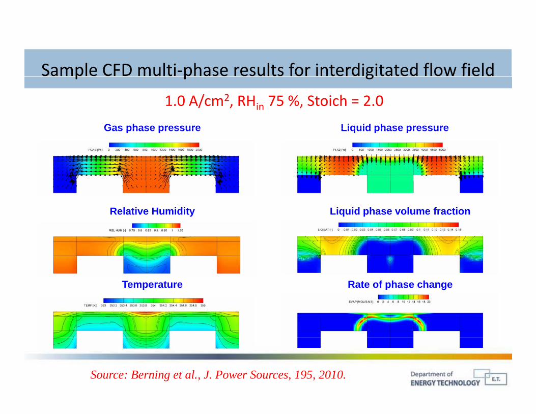
Sample CFD multi‐phase results for interdigitated flow field
Gas phase pressure Liquid phase pressure
p p g
1.0 A/cm2, RHin 75 %, Stoich = 2.0
Gas phase pressure Liquid phase pressure
Relative Humidity Liquid phase volume fraction
Temperature Rate of phase changeTemperature Rate of phase change
Source: Berning et al., J. Power Sources, 195, 2010.
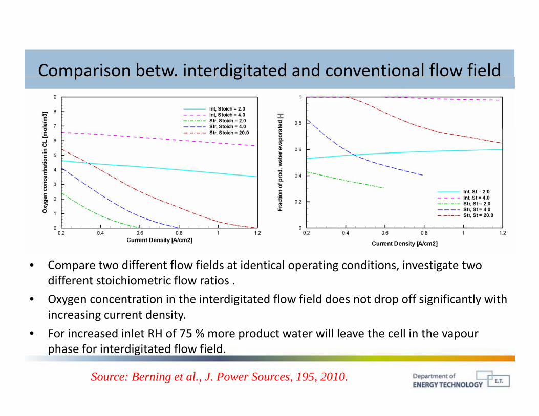
Comparison betw. interdigitated and conventional flow fieldp g
• Compare two different flow fields at identical operating conditions, investigate two different stoichiometric flow ratios .
• Oxygen concentration in the interdigitated flow field does not drop off significantly with increasing current density.
• For increased inlet RH of 75 % more product water will leave the cell in the vapour p pphase for interdigitated flow field.
Source: Berning et al., J. Power Sources, 195, 2010.
Other notable publicationsp
• Additonal publication of CFD models for fuel cells include:
• GurauGurau
• Djilali
• Mazumder and Cole (CFD ACE)
• (MANY more)• … (MANY more)
Conclusions I
• CFD is a powerful tool for modeling three‐dimensional, time
dependent multi‐phase and multi‐species transport
phenomena in flow channels and porous media that can:p p
Significantly reduce the number of experiments and hence safe cost
and time and decrease the time to market of a new productp
Significantly improve the fundamental understanding of transport
phenomena as they occur e.g. in a fuel cellp y g
Help to optimize the design and operating conditions of PEFC

Conclusions II
BUT
• Nearly all published CFD models of a fuel cell have insufficient physical y p p ymodels implemented because of a lack of fundamental understanding.
• A CFD model is only as good as its equations!
• There has been a bit of ”overselling” of (mostly commercial) fuel cell CFDThere has been a bit of overselling of (mostly commercial) fuel cell CFD models.
• There is the danger of conducting ”Colourful Fluid Dynamics”: It is easy to obtain a solution with today’s commercial CFD tools, and the user has toobtain a solution with today s commercial CFD tools, and the user has to be very critical with his/her own results and ensure that this is the right solution to the problem.
It is a very good practice to use a CFD model for the design of experiments: Try to identify a critical material parameter for fuel cell operation and help to design the right experiment in order to verify CFD finding.to design the right experiment in order to verify CFD finding.