MULTIPERIOD PLANNING AND UNCERTAINTY ISSUES IN CELLULAR

MULTI-PERIOD PLANNING AND UNCERTAINTY ISSUES IN

CELLULAR MANUFACTURING: A REVIEW AND FUTURE

DIRECTIONS

Jaydeep Balakrishnan,

Operations Management Area,

Haskayne School of Business,

University of Calgary,

Alberta T2N 1N4 Canada

Ph: (403) 220 7844 Fax: (403) 210 3327

Internet: [email protected]

Chun Hung Cheng

Department of Systems Engineering and Engineering Management,

The Chinese University of Hong Kong,

Shatin, Hong Kong, PRC

Internet: [email protected]

Author for correspondence: Jaydeep Balakrishnan

Published in the European Journal of Operational Research, 177, 2007, pp 281-

309.

2



DIRECTIONS

Abstract

In this paper we review research that has been done to address cellular manufacturing under

conditions of multi-period planning horizons, with demand and resource uncertainties. Most

traditional cell formation procedures ignore any changes in demand over time caused by product

redesign and uncertainties due to volume variation, part mix variation, and resource unreliability.

However in today‟s business environment, product life cycles are short, and demand volumes

and product mix can vary frequently. Thus cell design needs to address these issues. It is only

recently that researchers have been modelling uncertainty and multi-period issues. In this paper

we conduct a comprehensive review of the work that addresses these issues. We present

mathematical programming formulations as well as a taxonomy of existing models. Finally we

suggest some directions for future research.

Keywords: Facilities planning and design, manufacturing, flexibility, robustness, product life

cycle

3



DIRECTIONS

1.0 INTRODUCTION

In order to be successful in today's competitive manufacturing environment, managers have had

to look for new approaches to facilities planning. It is estimated that over $250 billion is spent

annually in the United States alone on facilities planning and re-planning (Tompkins et al.,

2003, p10). Further, between twenty and fifty percent of the total costs within manufacturing are

related to material handling and effective planning can reduce these costs by ten to thirty percent

(Tompkins et al., p10). Thus considerable benefits may be obtained from effective and

innovative approaches. These benefits are discussed in papers such as Meller and Gau (1996)

and Benjaafar et al. (2002). One innovative approach to facilities planning is called Group

Technology (GT). GT is based on the principle of grouping parts into families based on

similarities in design or manufacturing. This paper focuses on cellular manufacturing systems

(CMS), an important application of GT.

Manufacturing cells are created by grouping the parts that are produced into families. This is

based on the operations required by the parts. These cells, which consist of machines or

workstations, are then physically grouped together and dedicated to producing these part-

families. Cells combine the advantages of flow shops and job shops with characteristics such as

reduced cycle times compared to jobs shops and increased flexibility and greater job satisfaction

4

as compared to flow shops. A recent example of CMS implementation at Canon is reported in

Dreyfuss (2003). Canon, a major electronic equipment maker with 54 plants in 23 countries

manufacturing cameras, printers and copiers, recently implemented CMS in all of its assembly

lines. As a result, work-in-process (WIP) inventory in its factories has been reduced from three

days to six hours. Factory operating costs have been reduced by US$ 1.5 billion. Canon has

decreased its real estate costs by $279 million because cells require less room, and because the

reduced inventory level has resulted in fewer required warehouses (down from thirty seven to

eight).

CMS have some disadvantages however. Machines utilization may be lower due to dedication.

Significant training is required in order to operate cells effectively. Further, when system

uncertainty is present and product life cycles are short, cell reconfiguration may be an issue.

Various approaches have been suggested for forming manufacturing cells. Good discussions of

CMS can be found in Burbidge (1963), Suresh and Meredith (1985) and Selim et al. (1998).

Techniques range from the simple to the sophisticated and flexible. The simple techniques

usually manipulate part-machine matrices. The sophisticated ones can handle many constraints in

forming cells such as maximum cell size, different demands for different products, number of

cells and set-up costs.

However, most of these methods assume that the part demand stays constant over long periods

of time. But in today's market based and dynamic environment, part demand volume and part

5

mix can change quickly. Agility is required. For example, 75% of Hewlett Packard‟s (HP)

revenues are from product models that are less than three years old, and this percentage is

increasing (Hammer, 1996, p212). In fact HP now uses specialized forecasting methods for its

short life cycle products since traditional forecasting methods are no longer sufficient (Burruss

and Kuettner, 2003). In a study of thirty two manufacturing cell life cycles at fifteen plants,

Marsh et al. (1997) found that layout changes could occur as soon as within six months of the

start of the cell life cycle. Thus when manufacturing cells are created, expected changes in

products as well as uncertainty in demand and product mix have to be considered.

In this paper we review and categorize research that has been done to address cell

reconfiguration and uncertainty issues in CMS. We first describe a deterministic model where we

anticipate planned changes for the CMS due to planned product changes. We then discuss

research that addresses this issue. Subsequently we discuss the issue of uncertainty in demand or

product mix and the different approaches that can be used to address these issues. Finally we

identify some directions for future research. Figure 1 shows our categorization of the different

issues that exist in this area. We have also used this framework to guide the discussion of the

different research studies that have been done. The categorization of the various research papers

that have been published in this area is found in the Appendix, ordered by category. Some

research of course may fall in more than one category.

This paper is written to meet the needs of researchers and practitioners who wish to study CMS

under dynamic conditions. It helps decision makers understand the tradeoffs between the

6

different models that have been proposed and choose the appropriate technique for their

situations.

Figure 1: Categorization of multi-period planning and uncertainty issue in CMS

Multi-period Planning and Uncertainty Issues in Cellular Manufacturing

Multi-period Planning with Cell Reconfiguration

Uncertainty in Product Mix and Volume

Robust Designs General Facility Layout Cellular Manufacturing Robust Multi-period Plans Part Reallocation Fractal Layout Virtual Manufacturing Cells Concept and Design Distributed Layout Holonic Layout Hybrid Cells Modular Layout Routing Flexibility Multi-objective System Selection

7

2.0 MULTI-PERIOD PLANNING WITH CELL RECONFIGURATION

2.1 Problem Formulation and Past Work

As stated, shorter product life cycles are an increasingly important issue in cellular

manufacturing. One cannot assume that the designed cells will remain effective for a long time.

Ignoring the planned new product introductions would necessitate subsequent ad-hoc changes to

the CMS causing production disruptions and unplanned costs. Thus one has to incorporate the

product life cycle changes in the design of cells. This type of model is called the multi-period

CMS. In this model, we assume that a reasonable forecast of new product introductions, and part

mix or volume changes can be made so that a multi-period plan is possible. For a review of the

general multi-period layout planning models see Balakrishnan and Cheng (1998).

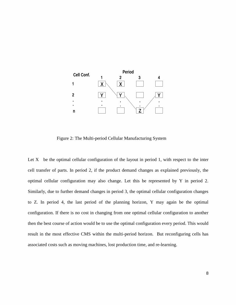
An example of a four period cellular manufacturing problem based on the dynamic plant layout

model of Rosenblatt (1986), is shown in Figure 2.

8

PeriodCell Conf.

Figure 2: The Multi-period Cellular Manufacturing System

Let X be the optimal cellular configuration of the layout in period 1, with respect to the inter

cell transfer of parts. In period 2, if the product demand changes as explained previously, the

optimal cellular configuration may also change. Let this be represented by Y in period 2.

Similarly, due to further demand changes in period 3, the optimal cellular configuration changes

to Z. In period 4, the last period of the planning horizon, Y may again be the optimal

configuration. If there is no cost in changing from one optimal cellular configuration to another

then the best course of action would be to use the optimal configuration every period. This would

result in the most effective CMS within the multi-period horizon. But reconfiguring cells has

associated costs such as moving machines, lost production time, and re-learning.

9

So the reconfiguration decision should be taken only after a cost-benefit analysis. Further, using

the wrong CMS configuration in a period may result in excess reconfiguration costs in

subsequent periods. Thus there are two types of conflicting costs and the objective in

determining a multi-period cellular configuration plan is to minimize the sum of these over the

planning horizon. Due to reconfiguration costs, it is possible that a sub-optimal cellular

configuration is the best one to use in a period as using this sub-optimal cellular configuration

might result in lower reconfiguration and overall costs. For example, cellular configuration X

may be optimal in period 2, but we use configuration Y because it lowers the overall multi-

period cost. Since a sub-optimal cellular configuration may be used in a period, we have to

examine every possible cellular configuration implicitly or explicitly in order to ensure overall

optimality. Thus, when creating manufacturing cells it is important to take into account not only

the interactions between machines but also the changes in product demand. Otherwise the cells

may become outdated quickly resulting in excess costs.

Wicks and Reasor (1999) identify three common objectives to be met when designing the multi-

period CMS, i.e., 1) minimizing the inter-cell transfer of parts, 2) minimizing duplication of

machines, and 3) minimizing the between-period reconfiguration of cells. Subcontracting firms

are good candidates for this model as these firms produce a variety of parts for a number of

customers (Drolet et al. 1996). The integer programming formulation of Wicks and Reasor is

shown below. Let

10

i = index of parts, i = 1, 2, …, N;

j = index of machines, j = 1, 2, …, M;

k = index of cells, k = 1, 2, …, C;

l = index of periods, l = 1, 2, …, P.

System parameters:

Dil = demand (production volume) for part i in period l;

Sil = number of processing operations for part i in period l;

O(i,r,l) = machine type required by the rth operation on part i in period l;

Tijl = processing time of part i on machine type j in period l;

Mj = number of type j machines available at start of planning horizon;

Cj = capacity of machine type j;

Pjl = cost of acquiring a type j machine in period l;

Hil = intercell per unit material handling cost for part i in period l;

Rjl = cost of relocating machine type j in period l;

LM = minimum number of machines per cell;

LP = minimum number of parts per family;

A = a large number

Decision variables:

xikl = 1 if part i is assigned to cell k during period l; 0 otherwise;

yjkl = 1 if machine j is assigned to cell k during period l; 0 otherwise;

njkl = number of type j machines assigned to cell k during period l.

qil = number of inter-cell transfers that occur during the production of

part i during period l;

bjl = number of additional type j machines acquired at the beginning

of period l;

ujl = number of type j machines that are relocated between period

(l – 1) and period l.

The objection function and system constraints can be formulated as follows:

.)()()(min1111

jljl

M

j

jljl

M

j

ililil

N

i

P

l

uRbPqDHZ (1)

where

.,)1(1

1

1),1,(),,(

liyyxqC

k

klOklO

S

r

iklil lrilri

il

(2)

11

.,,0max1

1

1

ljbMnbC

k

l

s

jsjjkljl (3)

.,}],0[max{ )1(

1

ljbnnu jlljkjkl

C

k

jl (4)

subject to:

C

k

ilikl liDx1

.,},0{min (5)

.,,1

lkjnCyxTD jkljjkliklijlil

N

i

(6)

N

i

C

k

jkljijlil ljnCTD1 1

., (7)

M

j

jkl lkLMy1

., (8)

N

i

ikl lkLPx1

., (9)

.,, lkjAyn jkljkl (10)

.,,,}1,0{, lkjiyx jklikl (11)

.,,,integer,0 lkjin jkl (12)

The overall objective of the formulation is to minimize the total system cost (Equation (1)). The

total system cost consists of the material handling cost (first term in the objective function),

capital investment (second term), and relocation costs (third term). Equation (2) describes the

inter-cell transfers per part, in a period. Equation (3) shows the number of machines acquired for

12

each period in the planning horizon. Equation (4) states the number of machines relocated for

each period in the planning horizon. Constraint (5) ensures that each part is assigned to exactly

one primary cell and that a part is only assigned to a cell for periods in which demand exists for

the part. Constraint (6) is the within-cell capacity constraint stating that the total capacity of

each machine type assigned to a cell must be sufficient to process the part family assigned to the

cell. Constraint (7) checks the entire system capacity. Constraints (8) and (9) enforce lower

limits on the number of machines and the number of parts assigned to each cell. Constraint (10)

ensures that the number of units of a given machine type in a cell is equal to zero unless the

machine type has been assigned to the cell. Finally, the values of the decision variables are

restricted by constraints (11) and (12).

Since the problem is nonlinear and difficult to solve for practical sizes, Wicks and Reasor

suggest a genetic algorithm (GA) approach. The chromosome used in the algorithm is based on a

single-period assignment of machines to cells. Within each period, each chromosome is further

divided into cells. A part-to-cell assignment heuristic that minimizes the inter-cell travel is also

used. The reproduction operator is a variation of the remainder stochastic sampling with

replacement policy. The crossover operator uses a standard single- and two-point method. Some

less fit children are allowed to survive and some mutation is allowed to provide diversity. The

GA is validated against other existing single period procedures using standard test problem data

sets and is shown to be effective.

13

They compare their method with a static CM approach using an illustrative problem. In the static

method the cell is designed using the first-period demand only and there are no further

rearrangements. When the part mix changes the new parts are introduced into the existing CMS

based on minimizing the inter-cell transfers of parts. Results show that the multi-period approach

with a planned rearrangement of cells performs better than the static situation.

Balakrishnan and Cheng (2005) suggest a two-stage method to solve this problem. Based on

Figure, 1, the static CMS and rearrangement of the CMS are separated so that each is solved

separately. Thus it is flexible in that the decision maker can use different preferred methods for

each stage. In the paper the authors use a GA for the static phase and dynamic programming for

the dynamic phase, but point out that any method may be used. They also do some sensitivity

analysis in the dynamic phase to illustrate the use of the dynamic approach in helping to improve

the CMS.

Drolet et al. (1996) briefly mention the development of a dynamic cellular manufacturing system

(DCMS) as part of their discussion on the evolution of cellular manufacturing. This model trades

off the cost of material handling and the cost of cell reconfiguration. In a subsequent paper in the

same journal issue Rheault et al. (1996) expand on the Drolet et al. (1996) model. The system

involves part routing and loading, and production scheduling and monitoring. This integer

programming model of the DCMS also trades off material handling cost and reconfiguration.

However it is not a multi-period integrated model. The model reconfigures the CMS based on

current period demand as needed. Marcoux et al. (1997) compare DCMS model of Rheault et al.

14

to a conventional CMS (CCMS) using a case study. In the study it is assumed that the planning

horizon is two weeks, but at the end of each week, the cells in DCMS (but not the CCMS) could

be reconfigured if necessary. The costs are calculated based on a 10 week study and the DCMS

proved significantly less expensive.

3.0 UNCERTAINTY IN PRODUCT MIX AND VOLUME

3.1 Problem Formulation

While the Wicks and Reasor model can be applied to situations where the plan for new product

introductions, and product mix and volume variation, can be reasonably forecasted, in many

cases uncertainty may exist. Consider the Canon example discussed at the beginning of the

paper. Usually customers demand some sort of customisation in products such as printers and

copiers. So manufacturers tend to run mixed-model assembly lines. Thus when designing a cell,

it has to be ensured that the cell is effective for different models (varying part mix) and uncertain

volume since it is often difficult to predict how successful a particular model will be.

Additionally there may be resource uncertainties such as machine breakdowns.

The formulation of Harlahakis et al. (1994) is one approach to addressing this uncertainty. This

formulation is discussed here. The cell formation problem consists of dividing the manufacturing

shop into a set of manufacturing cells C = {c1,…, cw}, such that the total inter-cell traffic of parts

within the design time horizon H is minimized. The definitions in the formulation are given

below where underlined characters indicate random variables.

16

Equation (13) ensures that on average the resulting machine-to-cell partition will yield the

minimal inter-cell traffic. Traffic values with higher probability are weighted more by this

criterion, while the entire range of feasible production volumes is considered. The first

constraint (equation 14), maintains the cell size below a predefined upper bound Q. The second

set of constraints (equation 15) reflects the limited machine capacities. The workload depends

on the set-up and run times of the make products and their production volumes. In the following

sections, different approaches to solve this and similar problems are discussed.

In the two models discussed it is assumed that explicit and implicit cost parameters are known.

However this may not always be true in practice. For example, as machines become more

technologically advanced, it is possible that moving them may become more expensive. One

may not be able to predict these costs in advance. Further the cost of acquiring the machine itself

17

may vary. On the one hand they may become cheaper as the technology matures but the cost of

inputs (such as steel required to make them) may be unpredictable. Further the material handling

costs also may not be predictable given the rate of technological change. Thus it is important to

examine the sensitivity of decisions to changes in these parameters. Robust designs are another

approach.

3.2 Robust Designs

The notion of robustness is initially studied in the general layout literature but can be adapted to

CMS. The robustness of a layout is an indicator of its flexibility in handling demand variability.

3.2.1 General Facility Layout

Shore and Tompkins (1980) use a regret cost criterion to design robust layouts. Given a set of

demand scenarios and associated probabilities of occurrence, penalty costs (regrets) are

calculated for candidate layouts across these scenarios. The most robust layout is considered to

be the one with the lowest expected facility penalty. Rosenblatt and Lee (1987) measure

robustness by whether a designed layout is within a Δ% of the optimal solution for every

possible demand scenario. Under uncertainty, it may be better to choose a layout which performs

well under all possible situations rather than one that is optimal for one possible scenario (which

may not occur) but does poorly in other possible scenarios.

Kouvelis et al. (1992) address the problem of uncertainty by using the concept of robust layouts.

Their method involves using a branch and bound (B&B) procedure (terminated before optimality

in large problems) for finding a list of solutions in each period that is within Δ% of optimality. In

18

another version of the stochastic layout problem, Rosenblatt and Kropp (1992) convert demand

scenarios and associated probabilities of occurrence into one weighted flow matrix to solve the

problem. Tests shows that this solution is robust giving good solutions in over 25,000 different

scenarios.

Yang and Peters (1998) consider a multi-period model with alternate production scenarios and

associated probabilities. The problem is solved deterministically using a mathematical

programming formulation that uses the weighted flow matrix where the weights are the

probabilities. In their model a rolling multi-period horizon is used where the layout can be

rearranged at the end of each period. They consider different time horizons from zero to time

period T to find the best time horizon. If the time horizon considered is short, the layout is

rearranged more frequently (called a flexible layout plan), while if it is T, then it is a „robust‟

layout since the same layout is used for the entire planning horizon. Thus, it is considered

appropriate for the different demand scenarios in each period. Tests show that the flexible layout

reduces inter-cell transfer cost compared to the robust layout.

Afentakis et al. (1990) model a flexible manufacturing system using simulation. The main

objective of the research is to compare a strategy of reconfiguring a layout every n periods

(periodic policy) with a strategy of rearranging it when the product volume, product mix or

product routing changes by a threshold percentage value (threshold policy). The volume of

parts and stability of this volume along with the frequency of change in the part mix are also

considered. In this research, the authors use material handling and reconfiguration costs as

19

separate measures of performance. The results show that given a dynamic situation, the material

handling performance deteriorates as n increases in the periodic policy and as the threshold

percentage increases. Also when the part mix changes, the threshold policies work better than the

periodic policies. Overall, the results show that a poor layout can add as much as 36% to the

material handling requirements. Therefore, given that FMSs are installed to perform better than

job shops or dedicated lines under conditions of uncertainty, it is important to monitor them

continuously on a layout basis to ensure its efficiency.

3.2.2 Cellular manufacturing

In CMS, Tilsley and Lewis (1977) address the issue of uncertainty in demand by using a

„cascading‟ strategy. A cascading system of cells is one where each cell is a child of another

cell. The child cell consists of some machines similar to those of its parent cell along with some

additional machines. If variable demand or mix changes result in the parent cell not being able

to cope, the parts can be rerouted to one of the child cells giving the CMS flexibility.

Seifoddini (1990) incorporates probabilistic demand in designing the CMS. Each product mix

and the related part-machine matrix are assigned probabilities. For each product mix considered,

the best cell configuration is determined. Subsequently for each of these best cell configurations

the expected inter-cell material handling cost based on possible product mixes is determined.

Finally that cell configuration with the lowest expected inter-cell material handling cost is

selected as the preferred CMS. This is considered a robust layout. Later Seifoddini and Djassemi

(1996) conduct a simulation study of a CMS where the part mix changes to illustrate the

20

sensitivity of the CMS to part mix changes. This sensitivity analysis can help the decision maker

predict the performance of a CMS under uncertainty.

Harlahakis et al. (1994) also consider product demand changes during a multi-period planning

horizon. They focus on robust cells by designing a cellular configuration using mathematical

programming based on expected values that would be effective over the ranges of demand

during multiple periods. Once the cells are designed they are expected to remain unchanged

during the multi-period horizon.

Marsh et al. in their survey of cell manufacturing life cycles discuss firms‟ „hard and soft

coping mechanisms‟ in dealing with environmental changes in a CMS. Examples of hard coping

mechanisms include the use of numerically controlled machining centres and tooling upgrades.

Example of soft coping mechanisms would be worker cross-training and set-up reduction.

3.2.3 Robust Multi-period Plans

Montreuil and Laforge (1992) consider a set of probabilistic future scenarios in designing the

layout. Initial skeletons are proposed and the relative positions of the departments do not change

in later periods. Only the shape and sizes of the departments change. As well the size of the

facility may also change. While these initial skeletons may appear to restrict the model, the

authors suggest an interactive approach in which different skeletons for the different futures can

be used. This is possible as the model is linear and thus large problems can be solved. The model

21

gives the resulting optimal layout for each future scenario in the scenario tree. The authors

suggest testing the robustness of the proposed layout tree by by performing sensitivity analyses

on aspects such as the probabilities of occurrences of each future, the design skeleton, and the

structure of futures of the tree.

Palekar et al. (1992) extend the product life cycle based work of Rosenblatt (1986) by

considering the stochastic dynamic plant layout problem where they convert different demand

scenarios into one weighted (by probabilities) flow matrix.

3.3 Part reallocation

Petrov (1968) addresses the issue of part mix changes in CMS by describing procedures used in

the former Soviet Union. He describes an algorithm that allocates the new demand to existing

cells. Though he indicates that issues such as common set ups should be considered in this

allocation, his algorithm does not consider these issues.

Vakharia and Kaku (1993) incorporate long-term demand changes into their 0-1 mathematical

programming cell design method by reallocating parts to families to regain the benefits of

cellular manufacturing. New parts are allocated to existing cells. So cells are not rearranged in

their multi-period design. While they discuss the possibility of partial or complete cell redesign

they do not adopt these strategies, to avoid system disruption. They formulate this problem

using an integer programming model. Since the problem is difficult to solve optimally it is

solved heuristically using a limited enumeration method. The method is validated using pilot

22

problems where the optimal solutions are obtained. The results show that the heuristic is

effective and efficient.

They also conduct a detailed experiment using seven existing data sets, three of which are

industry based. Stochastic part demand and processing times are generated using the uniform

distribution. The experiment consists of two parts. The first part examines the effect of factors

such as machine duplication cost, material handling cost, demand and mix changes, the number

of cells created and the routing flexibility (in terms of the ability of different cells to handle

different parts). It is found that changes in part volume require more duplication of equipment

than changes in part mix. Additionally if the CMS has low routing flexibility, changes in part

mix result in greater inter-cell movement than changes in part volume. This is reversed for high

routing flexibility. This indicates a tradeoff in handling volume changes versus mix changes.

The second part investigates robust designs by examining the effect of cell sizes and numbers on

robustness. Different volume and part mix levels are considered. In general the results show

that if the cell capacities in the initial preferred designs are not equal, then designs with larger

number of cells are more robust because they can handle different capacities. For designs with

equal cell capacity, fewer cells are more robust. This is as a result of less inter-cell movement.

For part mix changes, in addition to smaller number of cells, high routing flexibility also

contribute to robustness.

Askin et al. (1997) have proposed a four-stage algorithm that designs cells to handle variation in

23

the product mix. Initially a mathematical programming based method is used to assign operations

to machine types. Subsequent phases allocate part-operations to specific machines, identify

manufacturing cells, and improve the design. Experiments are also conducted to evaluate the

effect of factors such as utilization and maximum cell sizes on the effectiveness of the algorithm.

Again, cells once designed are expected to remain unchanged during the planning horizon.

3.4 Fractal Layout

Montreuil et al. (1999) and Venkatadri et al. (1997) discuss fractal layouts. A fractal layout

converts a functional layout into physical cells as in a conventional CMS. But unlike a

conventional CMS, the fractal layout procedure does not generally create cells based on product

families. Rather it uses the „factory within a factory‟ concept of Skinner (1974) with process

duplication. Figure 3 shows the example of a fractal layout where the four fractals in the layout

are identical. Thus all products can be processed in all the cells. However since having identical

fractals can result in unnecessary duplication or under-optimized flow performance, it may be

advisable to have fractals that are not identical (Montreuil et al., 1999). This is shown in Figure

4 where, though the fractals are similar, the layout within each fractal is different. As well,

machines are being shared. Thus in general, fractals will have the ability to produce a wider

variety of parts when compared to a traditional cell.

Montreuil et al. (1999) provide a conceptual discussion while Venkatadri et al. describe an

integrated mathematical programming approach for creating fractal cells. The steps involved in

24

creating a fractal layout include capacity planning (on aggregate), cell creation, flow assignment,

and cell and global layout. Montreuil et al. (1999) suggest setting the number of fractals a priori

to the minimum number of copies of any of the machines.

Figure 3: Identical fractal layouts

Source: Montreuil et al. (1999), International Journal of Production Research, reprinted with permission

from Taylor and Francis Ltd. (http://www.tandf.co.uk/journals).

25

Figure 4: Unidentical fractal layouts

Source: Montreuil et al. (1999), International Journal of Production Research, reprinted with permission

from Taylor and Francis Ltd. (http://www.tandf.co.uk/journals).

They also suggest allocating machines to cells such that the composition of each cell is roughly

equal. This leads to flexibility and can help respond to short term uncertainties such as machine

breakdowns and varying product mixes. If a fractal is unique for each product family then the

fractal layout basically becomes a pure CMS. Thus fractal layouts can range from a „factory

within a factory‟ concept to pure CMS.

http://www.tandf.co.uk/journals

26

Machines can be duplicated and shared if necessary to reduce inter-cell travel. Algorithms

similar to those used to solve the Quadratic Assignment Problem (QAP) are used in the cell and

global layout design phases. Montreuil et al. (1999) envisage that once a fractal layout is in

operation, physical cell separation need not be enforced. Rather some operational and control

mechanism such as a VCMS could be used. They also believe that fractal layouts provide great

flexibility and robustness. In summary, the fractal layout is an attempt to disperse workstations

throughout the facility in a meaningful way.

3.5 Virtual Manufacturing Cells

Many researchers have suggested the use of Virtual Manufacturing Cell Systems (VCMS) when

product demand is uncertain or unpredictable. In a virtual (logical) cell, machines are dedicated

to a product or a product family as in a regular cell, but the machines are not physically relocated

close to each other. The paper by McLean et al. (1982) is one of the first to propose such an

approach. An example of VCMS is shown in Figure 5.

27

Figure 5: A virtual manufacturing system

Reprinted by permission. Copyright 2002 INFORMS. Benjafaar, Saif, Sunderesh S. Heragu, Shahrukh A.

Irani. 2002. Next generation factory layouts: Research challenges and recent progress. Interfaces 32(6)

58--76, the Institute for Operations Research and the Management Sciences, 7240 Parkway Drive, Suite

310, Hanover, Maryland 21076, USA.

In a VCMS, machines in a functionally organized facility would be temporarily dedicated to a

part family. When a part requires processing it is routed to those machines dedicated to the part

family. Thus as in physical cells, dominant flow patterns arise. Machines in the virtual cell are

set up for that product family. If the demand pattern changes, the machines in any virtual cell

can be reassigned to another part family. Since no machines have to be moved, there is really no

rearrangement cost. This is an important advantage since using physical cells in the face of

uncertain demand might result in cells having to be rearranged frequently on an ad-hoc basis. If

the machines are not mobile, this could result in high costs (if the cells are reconfigured) or high

inefficiency (if the cells are not reconfigured).

28

Thus, according to Kannan and Ghosh (1996a) virtual cells are „flexible routing mechanisms‟.

Virtual cells combine the advantages of both process layouts and cellular manufacturing. For

example, one major disadvantage of traditional cellular manufacturing is that once cells are

formed, the machines in a cell may not be available for parts not dedicated to that cell. Thus the

machine utilization may suffer when compared to functional layouts, where machines can be

assigned to any part at any time. VCMS avoid this drawback as the machine allocations are only

temporary and can be reallocated easily (Prince and Kay, 2003). In addition in a VCMS, a

family could have access to multiple machines of the same type. Subsequently if the need arises,

some of these multiple machines can be reassigned to a part that needs it in order to ensure

equitable sharing of machines (Kannan and Ghosh, 1996a). One aspect where VCMS would not

have an advantage over physical cells is in the amount of travel since, in a virtual cell, the

layout remains functional and the part may have to travel larger distances within the virtual cell.

3.5.1 Concept and Design

Drolet et al. (1989) and Drolet and Moodie (1990) discuss algorithms and scheduling in VCMS

using production flow analysis (PFA), while Drolet et al. (1996) discusses VCMS within the

context of the evolution of CMS. Kochikar and Narendran (1998) describe a mathematical

programming based heuristic method to design a VCMS in an FMS.

Sarkar and Li (2001) using network optimization to design virtual cells where the objective is to

29

minimize throughput time. Instead of defining only one path they create the k best paths. In order

to achieve this they use a double sweep k-shortest path algorithm. A heuristic version of this

algorithm is devised to solve more practical scheduling situations with multiple jobs, shared

bottleneck machines, and precedence and resource constraints.

Ratchev (2001) describes an iterative and concurrent method for designing virtual manufacturing

cells through four steps. The first step involves identifying component requirements and

generating processing alternatives. Then the boundaries of the virtual cell capabilities are

defined, following which the machine tools are selected. The final step is system evaluation.

Prince and Kay (2003) discuss the use of virtual groups (VG) to enhance agility and leanness in

production. Both VCMS and VG use the concept that machines in a cell need not be physically

located close to one another. However, while VCMS focuses on managing the process, VG

focuses on the management of products from design to production. So the relationship of VCMS

to VG is somewhat analogous to the relationship between CMS and GT. GT is a much broader

concept than CMS and in fact includes CMS as its component. GT involves among other things,

part family identification, engineering design rationalization and variety reduction, and process

planning (Suresh and Meredith). Similarly in VCMS, it is assumed that the routing has been

provided and what is necessary is to identify the virtual cell required. There is no proactivity in

designing and process planning to make products fit into existing cells. The machines are

managed more like a jobs shop than a CMS, i.e, teams are directly in charge of machines or

machine groups but not products. Thus there would be handoffs from team to team in the

30

completion of a product which leads to discontinuities in the management of the production.

In a VG, as in GT, product group managers would be assigned a team of operators and all the

machines required (though physically distributed within the facility) to make complete products

or major subassemblies. They could be responsible for managing the product right from design,

through process planning, creation of the virtual cells and order completion. The advantage in

VG over VCMS is that VG is much more broad based and proactive in concept making planning

and scheduling more effective. Further Prince and Kay believe these groups are likely to be

longer lasting than in VCMS. This would make it easier to implement lean and agile concepts in

the different stages of production. In addition in VCMS, different machines in a group could be

managed by different groups, thus not utilizing the advantage of teams. Thus VG are an attempt

to improve upon some of the disadvantage of VCMS.

3.5.2 Comparison of VCMS to other Manufacturing Systems

In comparing VCMS to traditional CM, Subash Babu et al. (2000) categorize CM benefits into

three categories: (1) human related factor benefits from empowerment in smaller cells, (2)

improved flow and control in cells due to having to deal with smaller number of parts and

machines, and (3) improved operational efficiency due to similarities, in terms of reduced

setups, smaller batch sizes, increased quality, productivity, and agility. They suggest that VCMS

do not offer benefits in the first category, while providing considerable advantages in the second

31

and third categories.

Kannan and Ghosh (1996a, 1996b) compare different VCMS to CM and process layouts using

simulation. Different configuration rules for VCMS are considered. These include rules such

as: for a machine, giving allocation priority to a family with lower average slack per job, or to a

family with the fewest remaining machines needed to complete a cell. Inter-family setup times

are higher than intra-family setups as is common in practice. The demand patterns show

variability (uncertainty) through part mix and volume changes. Set up times and shop load are

also varied. Primary performance measures include mean flow time, mean tardiness and the

mean and standard deviation of the WIP.

The results show that VCMS perform better than both the process layout and CMS, over a wide

range of conditions and is more robust with respect to demand variability. When there is less

demand uncertainty, the cellular advantages of VCMS are utilized, while when demand

uncertainty is high, the VCMS‟ ability to quickly reconfigure the cells is utilized. The

simulation shows that VCMS allows jobs to spend less time in queues and setups as compared to

process layouts due to dedicated routings and shared family setups. It is also shown that some of

the VCM rules perform worse than the others. Kannan (1997) further investigates the effect of

family configuration on VCMS performance.

Vakharia et al. (1999) use queueing theory (using stochastic arrival and service rates) to

32

examine the performance of VCMS with multi-stage flowshops. The number of processing

stages, the number of machine copies at each stage, batch sizes and ratios of setup times to run

times per batch are varied. The virtual cells are manually created. In the VCMS setup time is

zero since each machine is a priori dedicated to a part family. In the multi-stage flowshop a part

may be routed to any of multiple copies of a machine in each stage. The results show that VCMS

are not always better that multi-stage flow shops with respect to flow times. For example, when

setup to run time ratios are high VCMS have an advantage as expected. But for large batch sizes

and greater number of stages, VCMS have higher flow times (poorer performance) than multi-

stage flow shops due to lack of routing flexibility and increased queue times. An industrial

application confirms the results that VCMS may not be appropriate for all stages. Rather a

combined system may work better.

While VCMS have advantages over CMS, it is unable to take advantage of some of the human

related factors as stated by Subash Babu et al. Human factor advantages are difficult to evaluate

through computer simulations such as that of Kannan and Ghosh (1996a, 1996b), and sometimes

tend to be overlooked. Important human factors aspects of CMS include team building, learning,

and problem solving. These would be difficult to do without physically grouping cells together.

For example, one company in the maintenance, repair and overhaul (MRO) industry that one of

the authors in familiar with uses CMS. Outside each cell, a board showing performance

indicators such as lead time, WIP, and bottleneck measures is posted. Thus any deterioration in

performance can quickly be identified and corrective measures taken. In a VCMS where

33

machines are not grouped together, such a posting would be difficult. In addition, in a VCMS,

just as in a process layout, it is not clear who would be responsible for improvement, since

employees work on individual machines and are not responsible for the entire routing. In CMS,

the team managing the cell would responsible for the performance.

HP (Hewlett-Packard, 1984) is another example of a company that uses CMS for facilitating

problem solving. Cell team members regularly spend time brainstorming and solving problems

within the cell to improve productivity and quality. This would be more difficult in a virtual cell

since team members may be working in different areas of the facility and may not work in

proximity to each other.

Thus VCMS is based on the recognition that in the current manufacturing environment of

uncertainty and short product life cycle, agility is important. VCMS in general appear to be more

agile than CMS. In terms of layout, the research on VCMS has usually assumed that the existing

job shop layout is not reorganized. However, as mentioned, physically grouping machines has its

advantages. Thus in the next sections we discuss three innovative layout approaches that have

been suggested in the literature that can facilitate the use of VCMS, while reducing some of the

disadvantages of VCMS. These include distributed, holonic and fractal layouts. All these layouts

involve some reorganization of the job shop layout but not as much as would be done is a CMS.

34

3.5.3 Distributed Layout

Benjaafar and Sheikhzadeh (2000) and Benjaafar et al. (2002) suggest that a distributed layout

might help in VCMS. In a distributed layout, machines of the same type are not grouped

together as in a process layout but they are distributed through out the facility individually or in

clusters. In a maximally distributed cell individual machines of the same type from a job shop

layout would be distributed uniformly in the facility as in Figure 6b. The maximally distributed

layout is the same in concept as a holonic layout proposed by Montreuil et al. (1993) which is

discussed in the next section. In a partially distributed layout each functional department is split

into subgroups and distributed throughout the facility and may have duplicate machines (Figure

6a). Thus when creating a virtual cell, the required machines from clusters that are located close

to each other can be selected. While still not a physical cell, the distance traveled by the part in

its routing can be reduced by using distributed layouts as compared with pure process layouts.

Earlier Figure 5 was used to illustrate a maximally distributed layout with virtual cells.

35

(a) Partially distributed layout (b) Maximally distributed layout

Figure 6: Distributed layouts





Benjaafar and Sheikhzadeh discuss a distributed layout model to design a flexible layout under

the conditions of varying product mix and product demand. They use mathematical

programming (heuristically) to minimize the material handling cost given different scenarios. In

this model the distribution of machines is not maximal. It is distributed based on the process

routing for products and the material flow between department types. Once set up, the control

would be similar to a VCMS where cells are created and disbanded as needed. Tests show that

this type of weighted layout performs better than both functional and maximally distributed

36

layouts. Thus it illustrates that including flow information in designing distributed layouts is

beneficial. They do caution that these benefits have to be traded off against losing the economies

of scale that exist in a job shop with respect to operators, loading/unloading, and computer

control which may have to be duplicated across all machine copies in a distributed layout.

Lahmar and Benjaafar (2002) extend this model for multi-period planning where the layouts can

be rearranged at the beginning of each period.

3.5.4 Holonic Layout

As mentioned, Montreuil et al. (1993) introduced a concept called holographic or holonic

layouts (Figure 6b). It is a subset of distributed layouts where individual machines are

distributed through the facility. It comes from the Greek words holos for whole and on for part.

The word holon was coined by Arthur Koestler (1968) to describe the basic unit of an

organization in a social or biological system. In a holonic layout, a machine (holon) that has no

duplicate would be placed in the center of the layout, while machines with more duplicates

would be strategically placed throughout the factory floor. The objective is to provide efficient

process routes for any part type that the system may need to produce with a minimum of delay.

Montreuil et al. (1993) describe a heuristic that attempts to spread machines of each type as

evenly as possible throughout the shop. As new orders arrive, routings are generated by

searching for compatibility between part requirements and machine availability, location, and

capability. Thus the operation and control is similar to VCMS. Like distributed layouts this

makes the layout robust in the face of agile environments. Marcotte and Montreuil (1995)

describe a procedure to form holographic layouts that assumes that information such as the

37

frequency of machine type to machine type transfers is known. These would be derived from the

process plans and demands. The process also includes selection of machine routings for products

as well as machine location.

Askin et al. (1999) compare process, holonic and fractal layouts using computer simulation. The

fractal layouts are selected to be identical as possible in the number and the type of machines.

The relative location of each machine in a fractal is random. In the holonic layout the machines

are either located throughout the facility randomly or by using a similarity coefficient method

where related machines are located close to each other.

Since incoming jobs have to be routed, different rules are considered, such as existing queues,

bottleneck avoidance or least total workload. For the fractal layouts, once a job goes into a fractal

it is completed in the fractal. In the holonic layout, static and dynamic (based on real time

information) rules are considered, where machine selection is based on existing queues and

travel time to candidate machines. For the process layout a job goes into a common queue for the

selected machine type. The layouts are simulated under various conditions of processing time,

move times, demand rates, plant sizes, number of processes, sequence selection, and utilization.

Cycle times are the primary performance measure.

The results provide insight into the comparative performance of different types of layouts. As

expected when move times are low process layouts perform better than holonic layouts. This

38

implies that process layouts are preferred to VCMS since holonic layouts are a form of VCMS.

In turn the similarity coefficient based holonic layout using dynamic scheduling rules performed

better than the fractal layout which is a form of CMS. This is due to the pooling effect of

common queues and the irrelevance of travel times due to its small magnitude. Thus if moves

can be done fast or move distances are short, then it appears that the flexibility of the traditional

process layout overrides the VCMS and CMS based attributes of the holonic or fractal layouts

respectively, at least in terms of cycle time.

For larger move times the fractal and holonic layouts performed better than process layouts. The

fractal layouts gave lower average cycle times than process layouts and holonic layouts, due to

the benefits of within cell processing similar to a CMS. Also choosing the fractal layouts based

on total workload, rather than number in queue or bottleneck avoidance provides better results.

However the similarity coefficient based holonic layout using dynamic routing rules was the

most robust, proving to be flexible and reliable under a variety of conditions.

Thus the holonic layout proved to be a good compromise between the flexible but longer travel

characteristics of process layouts and the less flexible but shorter travel characteristics of the

fractal layout which is more CMS like. Thus this research supports the notion that a VCMS is a

good compromise between process layouts and CMS. However, it was also shown that holonic

layout design was an important factor in its success since the random distribution if machines

resulted in poor results while the similarity coefficient based distribution gave good results. It

also appears that real time information in scheduling (deciding which machine to go to after it is

39

processed on the previous machine) is important for holonic layouts to be effective. This was not

an issue in fractal layouts, since as in a CMS, products sent to a fractal (cell) stay in that fractal.

Though partially distributed layouts have not been compared experimentally to holonic or

fractal layout, it is likely that the performance would depend on how „partial‟ it is. The more the

partially distributed layout is similar to a process layout, the more it is likely to be preferred to

holonic or fractal layouts for smaller move times. As seen in figure 6a, since each sub-group of

similar machines has multiple copies, the pooling effect of common queue as in a process layout

will be advantageous. If the layout is closer to the maximally distributed layout shown in Figure

6b, then it will have the advantages of a holonic layout which was effective for large move

times. As mentioned, in this case, actual distribution of machines as well as real time information

based scheduling is important.

3.6 Hybrid Cells

Irani et al. (1993) describe a hybrid CMS which retains some aspects of a functional layout while

at the same time allocates machines to part families. It allows for overlapping of routes, and

differing cell allocations to accommodate volume variation, machine breakdowns, mix changes

or other uncertainties. Thus it has characteristics of a VCMS also.

40

Figure 7: Types of layout: a) Functional Layout, b) Cellular layout c) Hybrid cells

Source: Gallagher, C.C., and Knight, W.A., 1973, Group Technology, London: Butterworth, p2,

(reprinted wth permission from Elsevier); Irani et al. (1993), International Journal of Production

Research, reprinted with permission from Taylor and Francis Ltd. (http://www.tandf.co.uk/journals)

Legend: T:Turning; M:Milling; D:Drilling; SG:Surface Grinding; CG:Cylindrical Grinding

41

Figure 7a shows a regular functional layout. In Figure 7b, the functional layout has been

converted into a CMS. One problem with the CMS is that if the part mix changes, the volume is

larger than expected or machines breakdown, then rerouting may become a problem. For

example assume that due to excess volume an additional drilling machine (D) is needed for the

cell with the square part. To access another D, the part may have to travel across two cells where

the closest D is located. This of course is not desirable from a material flow perspective. To

avoid this in Figure 7c, the cellular layout has been redesigned so that machines of the same type

are still close together as in a functional layout. For example, all D‟s are close together. So this

layout, called a hybrid layout provides the benefits of CMS and the routing flexibility benefits of

the functional layout. This also allows for flexibility by allowing machine to be allocated to

different part families in successive production periods through the use of tools and fixtures.

Thus it shares characteristics of a VCMS also, where the family-machine allocation changes

over time depending on the demand. Irani et al. (1993) also present an effective mathematical

programming based technique to design such cells. The benefits of hybrid layout is supported by

a survey by Wemmerlov and Hyer (1989). It shows that sharing of machines appeared to be

popular in practice with 20% of manned cells and 14% of unmanned cells in the companies

surveyed doing so.

Hybrid layouts have not been experimentally compared to the other types of layouts.

Conceptually, since it has the characteristics of a CMS, VCMS and process layouts it should be

flexible. If the demand tends to be uncertain in terms of product mix and volume, one could

avoid dedication of machines to part families and use it as VCMS with a process layout since the

42

layout involves characteristics of a process layout as shown in Figure 7c. On the other hand if

product demand is stable, it could be operated as a CMS. If move times are low it could be used

as a process layout as in Askin et al. (1999). Thus it could be used advantageously under various

demand conditions. The challenge would be to design the layout such that the layout can

physically have as much of the characteristics of a CMS and process layout as possible.

3.7 Modular Layout

Irani and Huang (2000) and Benjaafar et al. (2002) discuss modular layouts. A modular layout

consists of a network of modules, each representing part of the facility, and each of which could

be product, process or cell based. A product would have to move through one or more of these

modules to be processed. Figure 8 shows a modular layout at Motorola.

43

Figure 8: A modular layout at Motorola





The layout consists of different modules. Some are functional, while others are product based or

cell based. The modular design arises from the fact that ideally each product should be produced

in flow line which generally has the lowest cycle time. However this would result in too much

investment in machine duplication. The next best alternative is to identify subroutings within the

various products that are identical. These could then be produced on flow line as in high volume

manufacturing. This could form a flowline module. Naturally there could be multiple such flow

44

line modules if product line of the facility is large or machine duplication is viable. Where the

subroutings are not identical but have similar machine requirements, cell modules could be

created. These could then be identical to a CMS with its advantages. However unlike a

traditional CMS, note that only part of the product may be processed in a cell. Functional

modules are similar to a process layout and might include machines that cannot be duplicated

but are common to multiple part families. As in the process layout the routing of parts within the

functional module would be random. Benjaafar et al. suggest from experience that product

routings often have common substrings of operations that could be aggregated into flowline or

cell modules.

The physical layout could be designed so that products move between adjacent modules to avoid

unnecessary travel. If the product mix changes, the routing of a product between different models

would change. This might necessitate addition or deletion of modules as well as rearrangement

of the layout. Irani and Huang (2000) present mathematical programming formulation that

minimize the sum of inter-module travel and machine duplication. However since it is NP-

complete, they provide a heuristic method based on string matching and clustering using

similarities. They used the method to design a modular layout for Motorola. The advantage of

modular layouts is that they use the advantage of flow lines and cellular layouts as much as

possible while retaining the flexibility to produce different type of products or different volumes

efficiently.

45

3.8 Routing Flexibility

Gupta and Tompkins (1982) use simulation to study a CMS under the effect of part mix

changes and alternate routings. When a new order comes in, alternate routings (within and

outside cell) are considered if its regular routing will not allow it to be completed by the due

date. Rerouting to another cell results in a time penalty to reflect the ineffectiveness of the

alternate cell. After the completion of one operation the job continues on its original routing.

The results show that inter-cell moves are significantly lower for larger cell sizes since alternate

routings can be found within the cell. The authors caution that having very large cells would

result in both transportation and cell management disadvantages. An interesting observation is

that alternate routings may not always be advantageous. If the alternate route is inefficient, the

job may take more time. In this case it may be better to queue it in the most effective cell since

the queue times may be less than the additional process and transportation times incurred in

ineffective cells. However the results also show that queues tend to cause longer system

disturbances than alternate routings. The authors suggest a forward looking MRP system to help

plan re-routing ahead of time.

Ang and Willey (1984) compare hybrid cells to pure CMS using computers simulation. In a

hybrid CMS inter-cell transfer (alternate routing) is allowed. In their research design, if the

average workload at a machine exceeds a set threshold upon the arrival of another job at the

machine queue, a search is done to identify a suitable job that can be routed to another cell to

46

balance the overall workload. Different heuristics are used to identify this job. The job that is

moved to the other cell incurs additional material handling and is completed in the new cell if

possible. Different shop configurations and job dispatching rules are tested. Job mix and arrival

rates vary. Performance measures include mean job flow time, mean job tardiness, and the

standard deviation of mean job lateness.

Results show that inter-cell transfer, specifically at a low level, significantly improves

performance measurements under all conditions. Thus this inter-cell transfer allows the CMS to

respond better to part mix and volume variation. In addition batch overlapping (feasible in a

CMS due to the proximity of machines in a cell) works effectively in tandem with inter-cell

transfer. Thus hybrid cells prove to be more effective than pure cells.

Jensen et al (1996) compare three types of layouts – a functional job shop, a pure cell shop and a

„routing flexibility‟ (RF) cell shop. In the pure cell shop, all part operations are dedicated to a

single machine of a given type. All processing is completed within a single cell. There is no

routing flexibility. Thus it is similar to a product layout with dedicated machines and low set up

costs because of the dedication. An RF cell shop is a compromise between the functional shop

and pure cell shop. It has fewer cells than a pure cell shops, which implies that some cells can

have duplicate machines of the same type, as in a functional shop. But since each cell does not

process as many families as a functional shop, there is more dedication of machines leading to

lower set up costs and routing lower flexibility than the functional shop but more than a pure cell

shop.

47

The comparison is done using computer simulation under conditions of product mix and product

volume variability and the measures are flow time and tardiness. The results show that the RF

cell shop performs better than the other two types of shops under conditions of uncertainty. The

routing flexibility combined with the set up efficiencies makes it attractive. Thus the RF cell

design proves to be a robust design in the face of uncertainty in demand.

Albino and Garavelli (1999) investigate the concept of „limited flexibility (LF)‟ proposed by

Jordan and Graves (1995). In limited flexibility some alternate routing is allowed but not the

complete flexibility that would be allowed if each part could be processed by each cell. The

notion is to provide some flexibility to allow the system to be robust but at the same time to

avoid the additional investment and management complexity caused by complete flexibility.

The simulation study is done with demand mix variation and resource availability variation due

to factors such as machine breakdowns. Different loading rules are tested. The performance

measures are the cost of lost sales and total cost. The cells are designed using mathematical

programming. The results show that as system uncertainty increases, in general limited flexibility

is preferred to total flexibility. However the results are sensitive to the resource unreliability,

and the cost of adding routes versus the cost of lost sales.

48

Another way to achieve this flexibility is through the implementation of a flexible manufacturing

systems (FMS), i.e., a system with routing and processing flexibilities (Lin 1993, Ho and

Moodie, 1996). Studies by Lin , and Mehdi and Kurapati (1993) show that these systems can

yield significant productivity improvement. If a CMS uses such systems then each cell would

have much flexibility to handle uncertainties.

Meller and DeShazo (2001/2002) describe the implementation of Multi-channel Manufacturing

(MCM), a form of CMS where products are designed to have multiple routings, at an electrical

goods plant in the USA. The implementation of a cellular MCM (using some of the concepts of

Tilsley and Lewis) provides significant benefits over the previous process layout system.

3.9 Flexibility and Performance in Different Layouts

Routing flexibility is concept that relates of the layouts discussed so far. In fact many of layouts

and manufacturing systems discussed here have an implicit or explicit objective of improving

flexibility. The VCMS aims to increase flexibility by not physically reconfiguring cells. When

the product demand changes, logical cells are created from the process layout as required.

However as mentioned by Subash Babu et al. (2000), VCMS have the disadvantage that the

human factor benefits may be less than that of CMS. Further it is logical to assume that

improved human factor benefits may lead to increased flexibility in terms of producing multiple

products in a cell, learning, improved quality and ultimately faster through put.

49

Thus the implementation of a concept such as a VCMS can be enhanced by using innovative

layouts. The distributed layouts (Figure 6a and b) are examples of such innovative layouts. By

distributing the machines it may be possible to create cells such that the machines that process a

part family are close to one another thus in effect creating a CMS. Then at least some of the

advantages of the human factors aspects can be obtained. At the same time when product

demand changes the virtual cells can be rearranged without having to move equipment. Thus

distributed layouts may be useful where the cost of moving machinery is prohibitive. Where

machines can be moved at a reasonable cost then a multi-period model similar to Wicks and

Reasor (1999) can be used. The choice between different types of distributed layouts would

depend on the tradeoff between queue times and move times. If the queue pooling benefits of

partially distributed layout is more important than move times or human factor effects then it

would be preferred to maximally distributed (holonic) layouts. In the holonic layout since

individual machines are distributed more uniformly, there is a better likelihood than in the

partially distributed layout of finding a cell for a product where the machines are located in

close proximity. Thus would reduce move times and have better human factor advantages,

though queue times might be greater. Thus these layouts can provide different levels of

flexibility to a VCMS under different environments.

Similarly modular and hybrid layouts are an attempt to increase the flexibility of manufacturing

systems under conditions of uncertainty. As mentioned earlier hybrid layouts have characteristics

of process layouts as well as CMS. Thus depending on the situation they can be made to simulate

process layouts or VCMS. However further study would need to be done as to how effective it

50

would be in practice to create a layout as in Figure 7c where the machines are grouped into cells

while at the same time similar types of machines are in proximity of each other as in a process

layout. For example, one might want to examine if this sort of a layout be more feasible in a

larger facility with many machines or a smaller one. Also one might want to determine the ratios

the number of copies of each machine type should be in to make this feasible.

Modular layouts are different from the others in that it explicitly attempts to have different types

of traditional layouts within the same facility in order to improve flexibility. Conceptually

modular layout should be a good option for managers, perhaps better than the other proposed

layouts because of its combination of different layouts. None of other layouts proposed suggest

combining flowlines, cells and process layout. Thus, this combination should provide many

advantages. The flowline and cellular modules should help in reducing cycle times as opposed to

a process layout. In addition the existence of process modules should help it address the issue of

uncertainty. A one-off batch could be produced in the flexible process modules without affecting

the manufacture of products in the other modules much. Similarly product changes can be

accomplished by changing, adding or deleting modules without affecting the entire shop. The

challenge is to find common subroutings for flowline modules and to design robust cell modules

such that they can handle higher part variety without having to re-organize modules frequently.

On the other hand fractal cells are more similar to CMS in that they physically rearrange

machines into cells. But the objective is again to increase flexibility and the could use VCMS as

a control mechanism under uncertainty. As mentioned, if the cells are unique it becomes true

51

CMS with advantages and disadvantages. On the other hand if the cells are identical, a „ process

layout factory within a factory‟, the main benefit as seen by Askin et al. (1999) is in the low

travel times and in its flexibility in dealing with uncertainties such as machine breakdowns or

volume changes due to its process layout characteristics. However in the case of high uncertainty

in product mixes, the unidentical cell fractal layout may work better than the identical fractal

layout. Consider a hypthothetical Product 1 in an identical fractal layout (Figure 3) that is

routed through machines A, B and D of Cell 1 in that order. If there is a breakdown in Cell 1 or

the volume increases, since all the other three cells have an efficient A-B-D routing, the

environmental change can be handled efficiently. In the unidentical layout (Figure 4) only one

other cell has the A-B-D routing, and depending on the situation even this amount of duplication

may not exist. Thus it is not as effective as the identical fractal layout. However, if Product 1 is

replaced in the market by Product 2 requiring a routing of A-B-E, in Figure 3, such a routing

does not exist in an efficient manner while in the unidentical fractal layout (Figure 4), an

efficient A-B-E routing does exist in Cell 4. Thus in this case where the product mix has

changed, the unidentical fractal layout can handle this environmental change better than the

identical fractal layout. At the same time the identical fractal layout may be better than a true

process layout since the different types of machines may be in closer proximity as in Figure 3.

Thus cycle times will be faster and some the human factor advantages such team management of

the entire production of the part may also be possible. However, as Montreuil et al. (1999)

mention, an identical fractal layout may not be feasible because of excessive machine duplication

costs.

52

Thus in practice one may use a fractal layout that is a mix of unique and identical. This may

result in inter-fractal flows as shown in Figure 4. One important issue is in the design itself. In

the industrial case study done by Montreil et al. (1999), three fractal were created and each of

these could produce approximately one-third of the product line. This provided flexibility against

system breakdowns and presumably against product uncertainty. At the same time flow

reductions of 9% were achieved over pure CMS. Thus it appears that if fractal cells are properly

designed they can result in significant improvements in flexibility without sacrificing the

advantages of CMS such as low flow times. Another issue in fractal layout is that demand and

product mix uncertainty since physical cells are being created. Montreuil et al. (1999) suggest the

use of VCMS in operating and controlling the fractal cells, however they also suggest more

research into how this might be implemented.

3.10 Multi-objective System Selection

All the layouts discussed so far have been designed with a single objective in mind, usually the

minimization of the costs of material handling and machine investment. Moreover all the

measures have been quantitative. However, often there may be a combination of qualitative and

quantitative considerations in designing layouts. For example, while the human factor

advantages of different layouts has been discussed in this paper it had not explicitly been

modeled in any of the papers discussed. This aspect may be an important qualitative criterion in

designing layouts and could be incorporated by the use of multi-objective methods in layout

design.

53

Chan and Abhary (1996) combine cell formation methods, simulation and the Analytic

Hierarchy Process (AHP) to select the appropriate the cell design for an automated CMS. AHP

(Saaty, 1980) is a multi-objective decision support tool that uses specified weights and pair wise

comparisons of different alternatives based on competing multiple attributes. The authors

describe a case study in which four different cellular layouts are simulated to evaluate various

performance measures such as lead times, utilization, costs, reliability and flexibility. Three

cases with varying weights on the financial and non-financial attributes are tested. Some

attributes such as lead times could be compared on a pairwise basis directly from the simulation

results whereas interviews with plant personnel had to be done to make pairwise comparisons

for attributes such as flexibility. Based on these comparisons and using AHP software they are

able to determine the best manufacturing system. The same configuration is best in all three

cases, thus indicating the robustness of the solution.

4.0 FUTURE DIRECTIONS

One of the advantages of pure CMS is that workstations are designed to be in proximity of one

another, based on product flow. This opens opportunities for organizing teams of workers with

decision making responsibilities. Teams may be involved in production planning and scheduling,

quality management, and process improvement. As mentioned in the HP example, cell team

members regularly met to discuss productivity and quality improvements. Future research needs

to examine how these issues could be integrated with flexible cell design, which helps dealing

with demand and part mix variations, but where machines may not be physically located to next

to each other. Future case studies of the implementation of some of the procedures described in

54

this paper may shed lights on these issues.

Traditionally, there has not been much research in organizational behaviour issues in cellular

manufacturing. One reason may be that these concepts are difficult to model (Morris and

Tersine, 1990). However in recent years several researchers have highlighted the important

interactions between human resources management (HRM) and operations management (OM),

and the need to incorporate organizational behaviour issues in operations management.

Boudreau et al. (2003) discuss the interface between HRM and OM in various operations

management decisions. They provide references to previous work in the HRM/OM interface

and conceptual frameworks for incorporating HRM concepts in to OM and vice versa. A recent

special issue of Management Science (Volume 49, Number 4, April 2003) focused on creating,

retaining and transferring knowledge in organizations. Further, another special issue of IIE

Transactions (Volume 36, Number 10, October 2004) dealt with workforce agility. Finally

Boudreau (2004) presents a survey of papers that appeared in the first fifty years of the journal

Management Science related to organizational behaviour.

Fazakerley (1974) through studies at multiple facilities in the United Kingdom suggests that the

following personnel problems may occur when CMS is introduced: 1) uncertainty and insecurity,

2) management‟s lack of understanding of CMS, 3) lack of team work within cells, 4) tendency

to become complacent and less innovative, and 5) problems with the compensation system. One

could examine how these issues affect CMS innovations such as VCMS, holonic layout, or

distributed layout, which are more sophisticated concepts than a pure CMS.

55

Shafer et al. (1995) through a survey of employees at two manufacturing facilities compare the

effect on employee perception and attitude of cellular manufacturing versus functional

manufacturing. They find that cellular manufacturing has both positive and negative impact.

Although the positive aspects can be explained by the fact that CMS job characteristics such as

increased autonomy, flexibility, and responsibility increase job satisfaction, it is more difficult

to explain the negative aspects. Shafer et al. speculate that any job problems that may exist are

made more acute by CMS and that that some employees may have difficulty in adapting to CMS.

In essence they echo Fazakerley‟s concerns. For example, employees who are not motivated

towards growth in their career may not be ready to accept the uncertainty that accompanies

increased autonomy, responsibility and flexibility. Further, in a process layout employees tend to

work individually while in a CMS they tend to work in groups. If some employees are unable to

work in groups or the groups do not function effectively, the results may be increased

dissatisfaction on the part of these employees. Also if workers do not understand CMS concepts,

they may not be convinced of the benefits of CMS implementation, resulting in change

management issues.

One important aspect that has been shown to affect the performance of cellular manufacturing is

learning. Learning curve theory, a good survey of which is done by Yelle (1979), indicates that

the processing time required decreases with increases in repeated output. Thus the theory

suggests that since in a CMS there is more job repetition than a job shop, there may be more

learning and resulting shorter processing times in a CMS. Thus learning should be one of the

56

factors considered in comparing the two systems. Kannan (1996) shows that learning in a CMS

allows it to overcome the disadvantages or reduced flexibility due to machine dedication to part

families. Kannan uses the log-linear function (Wright, 1936) to model learning. Biskup and

Simons (2004) call the model using the log-linear function, „autonomous learning‟ while

learning models in which management is actively involved is called „induced learning‟. In

induced learning management incurs an initial investment such as employee training to stimulate

learning beyond the autonomous model. Biskup and Simons formulate and solve a mathematical

programming model that optimizes the amount of initial investment for learning required to

minimize earliness and tardiness. Kannan and Palocsay (1999) through the use of queueing

models show that without learning, manufacturing cells may perform poorly when compared to

job shops.

Researchers have also recently addressed an allied induced learning issue which is important in

CMS, that of cross training. Jordan et al. (2004) use queuing and simulation to evaluate different

cross training strategies for time required for completing repairs in the maintenance function.

Bokhorst et al. (2004) use goal programming and simulation to investigate different cross

training policies. In this paper the authors consider both HRM (minimizing the standard

deviation of workload) and OM (minimizing flow time) measures. Kula et al. (2004) use

queueing theory to model set-up operations with cross training and show that cross training has

a beneficial effect on flow times.

Since both learning and cross training serve to increase the effectiveness of CMS, it would be

57

useful to investigate the effect of these factors when uncertainty is considered. For example,

since virtual cells, hybrid cells and distributed, holonic, fractal layouts involve features of both

CMS and jobs shops but in different ways, it is important to evaluate whether learning and cross

training would have different effects under certainty and uncertainty. This could involve models

previously used to evaluate these issues in general manufacturing such as queueing theory,

computer simulation and mathematical programming. Also the impact of the incorporation of

learning and cross training on the solution methods used in multi-period CMS models discussed

in this paper is also an important issue. Furthermore, the importance of learning in cells depends

on the nature of processes such as postponement, modular design, and product standardization,

since they have different effect on the stability of CMS. This area requires future study.

One of the advantages of CMS is reduction in setups. Ensuring that setups do not become an

issue again as they are in process layouts, when flexible layout strategies such as distributed

layouts that handle part mix and demand changes are used, have to be investigated. This is

particularly important given the current focus on small lot sizes in agile manufacturing.

Comparison of dynamic cells (in which physical cells are reconfigured periodically) versus

robust cells (in which cells stay static and uncertainties are managed through strategies such as

VCMS) is needed to identify the conditions under which one would be favoured over the other.

Further, we saw in the Canon example that moving cellular manufacturing reduces the use of

conveyers and other material handling equipment. This is a main advantage for physically

58

grouped cells. However, it is conceivable that in layouts where cells are not grouped together

such as distributed or holonic cells, material handling systems may still be required. Thus the

equipment investment tradeoffs need to be made between pure CMS and non-physical CMS.

Another layout design issue that could be addressed in the future is that of lead times and its

variability in the procurement of resources, such as equipment from suppliers, in order to

redesign the layout. The longer this lead time is, the longer the forecast horizon for product

demand and mix has to be in order to plan new layouts for the expected demand changes. For

example if the lead time to acquire a machine is six months, it implies that one has to forecast at

least six months into the future to ensure that the machine can be acquired in time for the layout

redesign. If the lead time is one year, the forecast has to be made at least one year into the

future. The variability in this lead time also has an effect. For example if the mean lead time is

six months but the actual lead time varies between four months and eight months, to ensure that

layout redesign schedules are not disrupted, one may have to forecast up to eight months ahead,

in effect adding a safety time buffer. Forecasts further out have greater uncertainty. Thus this

lead time will have an effect on the accuracy of the layout redesign plans.

5.0 CONCLUSION

There has been much literature in the area of cellular manufacturing. Most of the research in this

area assume that cells once designed need not be redesigned for a considerable length of time.

However, with the advent of global competition and advancements in technology, life cycles of

products have become much shorter. As well, the greater desire for customized products has

59

resulted in the unpredictability in the volume and mix of the products that need to be

manufactured in these CMS.

Some recent work in CMS has started to address cell reconfiguration and uncertainty issues. In

this paper we have presented the basic problems in cell reconfiguration and uncertainty. Then we

briefly described the research and have organized it into categories. The categorization also

includes a summary. As seen, there have been a variety of innovative strategies and techniques

used in addressing these issues. The most popular innovative approach to CMS appears to be

virtual cells. Other methods include fractal cells and holonic cells. Solutions make use of

mathematical programming, simulation and, queueing theory as well as specialized cell

formation algorithms. As well there has been extensive studies by the different authors on the

conditions under which proposed strategies and techniques have been useful. Finally we also

identify some future areas for research.

Acknowledgements

This research was supported by grants from the Natural Sciences and Engineering Research

Council (NSERC) of Canada, and the Research Grants Council of the Hong Kong SAR, China

(Project No. 411205). The authors are also thankful to the anonymous reviewers and the editor

for their comments.

60

REFERENCES

1. Afentakis P., Millen, R.A., and Solomon, M.M. (1990), “Dynamic layout strategies for

flexible manufacturing systems”, International Journal of Production Research, 28, 2,

311-323.

2. Albino, V., and Garavelli, A.C. (1999), “Limited flexibility in cellular manufacturing

systems: a simulation study”, International Journal of Production Economics, 60-61, 447-

455.

3. Ang, C.H., and Willey, P.C.T. (1984), “A comparative study of the performance of pure

and hybrid group technology manufacturing systems using computer simulation

techniques”, International Journal of Production Research, 22, 2, 193-233.

4. Askin, R.G., Selim, H.M. and Vakharia, A.J. (1997), “A methodology for designing

flexible cellular manufacturing systems”, IIE Transactions, 29, 599-610.

5. Askin, R.G., Ciarallo, F.W., and Lundgren, N.H. (1999), “An empirical evaluation of

holonic and fractal layouts”, International Journal of Production Research, 37, 5, 961-

978.

6. Balakrishnan, J. and Cheng, C.H. (2005), “Dynamic cellular manufacturing under multi

period planning horizons”, Journal of Manufacturing Technology Management, 16, 5.

7. Balakrishnan, J. and Cheng, C.H. (1998), " The dynamic plant layout problem - a state-of-

the-art review”, OMEGA, 26, 4, 507-521.

8. Benjaafar, S. and Sheikhzadeh, M. (2000), “Design of flexible layouts”, IIE Transactions,

32, 309-322.

9. Benjaafar, S. Heragu, S.S. and Irani, S.A. (2002), “Next generation factory layouts: research

challenges and recent progress”, Interfaces, 32, 6, 58 -77.

10. Biskup, D. and Simons, D. (2004), “Common due date scheduling with autonomous and

induced learning”, European Journal of Operations Research, 159, 606-616.

11. Bokhorst, J.A.C., Slomp, J., and Molleman, E. (2004), “Development and evaluation of

crosstraining policies for manufacturing teams”, IIE Transactions, 36, 10, 969-984.

12. Boudreau, J.W. (2004), “Organizational behaviour, strategy, performance, and design in

Management Science”, Management Science, 50, 11, 1463-1476.

61

13. Boudreau, J., Hopp, W., McClain, J.O., and Thomas, L.J. (2003), “On the interface between

operations and human resource management”, Manufacturing and Service Operations

Management, 5,3, 179-202.

14. Burbidge, J.L. (1963), “Production flow analysis”, Production Engineer, 42, 742-752.

15. Burruss, J. and Kuettner, D. (2002), “Forecasting for short lived products: Hewlett

Packard‟s journey”, Journal of Business Forecasting, 21, 4, 9-14.

16. Chan, F.T.S., and Abhary, K. (1996), “Design and evaluation of automated cellular

manufacturing systems with simulation modeling and AHP approach: a case study”

Integrated Manufacturing Systems, 7, 6, 39-49.

17. Dreyfuss, J. (2003), “Profit Machine”, Bloomberg Markets, October, 29-38

18. Drolet, J., Montreuil, B., and Moodie, C. (1989), "Scheduling factories of the future",

Journal of Mechanical Working Technology, 20, 183-194.

19. Drolet, J. and Moodie, C. (1990), "A virtual cell scheduling algorithm", Progress in

Materials Handling and Logistics, 2, Springer-Verlag, 489-500.

20. Drolet, J., Abdulnour, G. and Rheault, M. (1996), "The cellular manufacturing evolution",

Computers and Industrial Engineering, 31,1/2, 139-42.

21. Fazakerley, G.M. (1974), “The human problems of group technology”, European Business,

Summer, 50-56

22. Gupta, R.M, and Tompkins, J.A. (1982), “An examination of the dynamic behaviour of

part families in group technology”, International Journal of Production Research, 20, 1,

73-86.

23. Hammer M. (1996), Beyond Reengineering, New York, NY: HarperCollins, 212.

62

24. Harlahakis, G., Ioannou, G., Minis, I, and Nagi, R. (1994), “Manufacturing cell formation

under random product demand”, International Journal of Production Research, 32, 1, 47-

64.

25. Hewlett-Packard Company (1984), “Stockless production”, HP-TV Network, 1891 Page

Mill Rd., Palo Alto, CA 94304.

26. Ho, Y-C, and Moodie, C.L. (1996), “Solving cell formation problems in a manufacturing

environment with flexible processing and routeing capabilities” International Journal of

Production Research, 34, 10, 2901-2923.

27. Irani, S.A., Cavalier, T.M, and Cohen, P.H. (1993), “Virtual manufacturing cells:

exploiting layout design and intercell flows for the machine sharing problem”,

International Journal of Production Research, 31,4, 791-810.

28. Irani, S.A., and Huang, H. (2000), “Custom design of facility layouts for multi-product

facilities using layout modules”, IEEE Transactions on Robotics and Automation, 16, 259-

267.

29. Jensen, J.B., Malhotra, M.K., and Philipoom, P.R. (1996), “Machine dedication and

process flexibility in a group technology environment”, Journal of Operations

Management, 14, 19-39.

30. Jordan, W.C., and Graves, S.C. (1995), “Principles on the benefits of manufacturing

process flexibility”, Management Science, 41, 4, 577-594.

31. Jordan, W.C., Inman, R.R., and Blumenfeld, D.E. (2004), “Chained cross-training of

workers for robust performance”, IIE Transactions, 36, 10, 953-967.

32. Kannan, V.R. (1996), “Incorporating the impact of learning in assessing the effectiveness

of cellular manufacturing”, International Journal of Production Research, 34, 12, 3327-

3340.

33. Kannan, V.R., and Ghosh, S. (1996a), “Cellular manufacturing using virtual cells”,

International Journal of Operations and Production Management, 16, 5, 99

34. Kannan, V.R. and Ghosh, S. (1996b), "A virtual cellular manufacturing approach to batch

production", Decision Sciences, 27, 3, 519-39.

35. Kannan, V.R. (1997), “A simulation analysis of the impact of family configuration on

virtual cellular manufacturing”, Production Planning and Control, 8, 1, 14-24.

63

36. Kannan, V.R., and Palocsay, S.W. (1999), “Cellular vs process layouts: an analytic

investigation of the impact of learning on shop performance”, OMEGA- International

Journal of Production Research, 27, 583-592.

37. Kochikar, V.P. and Narendran, T.T. (1998), “Logical cell formation in FMS using

flexibility based criteria”, International Journal of Flexible Manufacturing Systems, 10, 2,

163-181.

38. Koestler, A. (1968), The Ghost in the Machine, New York: Macmillan

39. Kouvelis, P., Kurawarwala, A.A. and Gutierrez, G.J. (1992), “Algorithms for robust single

and multiple period layout planning for manufacturing systems”, European Journal of

Operations Research, 63, 287-303.

40. Kula, U., Duenyas, I., and Iravani, S.M.R. (2004), “Estimating job waiting times in

production systems with crosstrained setup crews”, IIE Transactions, 36, 10, 999-1010.

41. Lahmar, M. and Benjaafar, S. (2002), “Design of dynamic distributed layouts”, Working

paper, Department of Mechanical Engineering, University of Minnesota, Minneapolis,

MN.

42. Lin, G.Y. (1993), “A distributed production control for intelligent manufacturing systems”,

Ph.D. Thesis, Purdue University, West Lafayette, Indiana.

43. Marcotte, S, and Montreuil, B. (1995), “Design of holographic layout for agile flow

shops”, Proceedings of the Productivity in A World without Borders Conference, Montreal,

929-938.

44. Marcoux, Y., Drolet, J., and Abdulnour, G. (1997), "Studying the performance of a

dynamic cellular manufacturing system”, Computers and Industrial Engineering, 31, 1-2,

239-242.

45. Marsh, R.F., Meredith, J.R., and McCutcheon, D.M. (1997), “The life cycle of

manufacturing cells”, International Journal of Operations and Production Management,

17, 12, 1167-1182.

46. McLean, C.R., Bloom, H.M. and Hopp, T.H. (1982), “The virtual manufacturing cell”,

Proceedings of the 4th

IFAC/IFIP Conference on Information Control Problems in

Manufacturing Technology, Gaithersburg, MD, 1-9.

64

47. Mehdi, K., and Kurapati, V. (1993), “Flexible manufacturing system: an overview”

International Journal of Operations and Production Management, 14, 4, 26-49.

48. Meller, R.D. and Gau, KY. (1996), “The facility layout problem: recent and emerging

trends and perspectives”, Journal of Manufacturing Systems, 15, 5, 351-366.

49. Meller, R.D. and DeShazo, R.L. (2001/2002), “Manufacturing System Design Case Study:

Multi-channel Manufacturing at Electrical Box and Enclosures” Journal of Manufacturing

Systems, 20, 6 445-456.

50. Montreuil, B. and LaForge, A. (1992), “Dynamic layout design given a scenario tree of

probable futures” European Journal of Operations Research, 63, 271-286.

51. Montreuil, B., LeFrancois, P., Marcotte, S., and Venkatadri, U. (1993), “Holographic

layout of manufacturing systems operating in chaotic environments”, Technical Report 93-

53, Document de Recherche GRGL, Faculte des Sciences de l‟Administration, Universite

Laval, Quebec.

52. Montreuil B., Venkatadri U., and Rardin, R.L. (1999), “Fractal layout organization for job

shop environments”, International Journal of Production Research, 37, 3, 501-521.

53. Morris, J.S. and Tersine, R.J. (1990), “A simulation analysis of factors influencing the

attractiveness of group technology cellular layouts”, Management Science, 36, 12, 1567-

1575.

54. Palekar, U.S., Batta, R., Bosch, R.M, and Elhence, S. (1992), “Modeling uncertainties in

plant layout problems”, European Journal of Operations Research, 63, 347-359.

55. Petrov, V.A. (1968), Flowline Group Production Planning, London: Business Publications

56. Prince, J. and Kay, J.M. (2003), “Combining lean and agile characteristics: creation of

virtual groups by enhanced production flow analysis”, International Journal of Production

Economics, 85, 305-318.

57. Ratchev, S.M. (2001), “Concurrent process and facility prototyping for formation of virtual

manufacturing cells” Integrated Manufacturing Systems, 12, 4, 306-315.

65

58. Rheault, M., Drolet, J. and Abdulnour, G. (1996), "Dynamic cellular manufacturing system

(DCMS)", Computers and Industrial Engineering, 31, 1/2, 143-146.

59. Rosenblatt M.J. (1986), “The dynamics of plant layout”, Management Science, 32, 1, 76-

86.

60. Rosenblatt, M. J., and Lee, H.L. (1987), “A robustness approach to facilities design”,

International Journal of Production Research, 25, 4, 479-486.

61. Rosenblatt, M.J., and Kropp, D.H. (1992), “The single period stochastic plant layout

problem”, IIE Transactions, 24, 2, 169-176.

62. Saaty, T.L. (1980), The Analytic Hierarchy Process, New York: McGraw Hill.

63. Sarkar, B.R. and Li, Z. (2001), “Job routing and operations scheduling: a network-based

virtual cell formation approach”, Journal of the Operational Research Society, 52, 673-

681.

64. Seifoddini, H. (1990), “A probabilistic model for machine cell formation”, Journal of

Manufacturing Systems, 9, 1, 69-75.

65. Seifoddini, H. and Djassemi, M. (1996), “Sensitivity analysis in cellular manufacturing

system in the case of product mix variation”, Computers and Industrial Engineering, 31,

1/2, 163-167.

66. Selim, H.M., Askin, R.G. and Vakharia A.J. (1998), “Cell formation in group technology:

review, evaluation and directions for future research”, Computers and Industrial

Engineering, 34, 1, pp. 3-20.

67. Shafer S.M., Tepper B.J., Meredith J.R. and Marsh R. (1995), “Comparing the effects of

cellular and functional manufacturing on employees‟ perceptions and attitudes”, Journal

of Operations Management, 12, 63-74.

68. Shore, R.H. and Tompkins, J.A. (1980), “Flexible facilities design”, AIIE Transactions, 12,

2, 200-205.

69. Skinner W. (1974), “The focused factory”, Harvard Business Review, 52, 113-121.

70. Subash Babu, A., Nandurkar, K.N. and Thomas, A. (2000), “Development of virtual

cellular manufacturing systems for SMEs”, Logistics Information Management, 13, 4,

228- 243.

66

71. Suresh, N.C. and Meredith J.R. (1985), “Achieving factory automation principles through

group technology principles”, Journal of Operations Management, 5, 2, 151-167.

72. Tilsley, R. and Lewis, F.A. (1977), “Flexible cell production systems – a realistic

approach”, Annals of the CIRP, 25, 1, 269-271.

73. Tompkins, J.A., White, J.A., Bozer, Y.A., and Tanchoco J.M.A. (2003), Facilities

Planning, New York: Wiley.

74. Vakharia, A.J., and Kaku, B.K. (1993), “Redesigning a cellular manufacturing system to

handle long-term demand changes: a methodology and investigation”, Decision Sciences, .

24, 5, 909-929.

75. Vakharia, A.J., Moily, J.P. and Huang Y. (1999), “Evaluating virtual cells and multistage

flowshops”, International Journal of Flexible Manufacturing Systems, 11, 3, 291-314.

76. Venkatadri, U., Rardin, R.L. and Montreuil B. (1997), “A design methodology for fractal

layout organization”, IIE Transactions, 29, 911-924.

77. Wemmerlov, U. and Hyer, N.L. (1989), “Cellular manufacturing in the US industry: A

survery of users”, International Journal of Production Research, 27, 9, 1511-1530.

78. Wicks, E.M and Reasor R.J. (1999), “Designing Cellular Manufacturing Systems with

Dynamic Part Populations”, IIE Transactions, 31, 11-20.

79. Wright, T.P. (1936), “Factors affecting the cost of airplanes”, Journal of Aeronautical

Sciences, 3, 4, 122-128.

80. Yang, T. and Peters, B.A. (1998), “Flexible layout design for dynamic and uncertain

environments”, European Journal of Operations Research, 108, p 49-64.

81. Yelle, L.E. (1979), “The learning curve: historical review and comprehensive survey”,

Decision Sciences, 10, 2, 302-328.

67

APPENDIX

Authors Year Category Tool

Selim, Askin, and Vakharia 1998 Review

Benjaafar, Heragu, and Irani

2002 Review

Rheault, Drolet, and Abdulnour 1996 Multi-period plan Mathematical

Programming

Drolet, Abdulnour, and Rheault 1996 Multi-period Plan

VCMS

Conceptual

Marcoux, Drolet, and

Abdulnour

1997 Multi-period plan

Conventional CMS

Case Study comparison

Wicks and Reasor 1999 Multi-period plan Genetic Algorithm

Balakrishnan and Cheng 2004

Flexible multi-

period plan

Genetic Algorithm

Dynamic Programming

Tilsley and Lewis 1977

Robust design Cascading cells

Shore and Tompkins 1980 Robust design

(facility layout) Specialized algorithm

Rosenblatt and Lee 1987 Robust design

(facility layout)

Conceptual

Decision Theory

Afentakis, Millen, and

Solomon

1990 Robust design

(FMS) Simulation

Seifoddini 1990 Robust design Clustering algorithm

Rosenblatt and Kropp 1992 Robust design

(facility layout)

Stochastic Mathematical

Programming

Kouvelis, Kurawarwala, and

Gutierrez

1992 Robust design

(facility layout)

Branch and Bound

68

Seifoddini and Djassemi 1996 Robust design Sensitivity analysis

Harlahakis , Ioannou, Minis

and Nagi

1994 Robust design Stochastic Mathematical

Programming

Marsh, Meredith and

McCutcheon

1997 Robust design, cell

life cycles

Survey

Yang and Peters 1998 Multi-period plan

Robust design

(facility layout)


Programming

Montreuil and LaForge 1992 Robust multi-

period plan (facility

layout)


Programming

Palekar, Batta, Bosch, and

Elhence

1992 Robust multi-

period plan

(facility layout)


Programming

Petrov 1968 Part reallocation

Robust design

Specialized Algorithm

Vakharia and Kaku 1993 Part reallocation

Robust Design

Mathematical

Programming

Experimental design

Askin, Selim, and Vakharia 1997 Part reallocation

Routing flexibility

Mathematical

Programming Graph Partitioning

Specialized algorithms

McLean, Bloom, and Hopp 1982 VCMS - Design

Conceptual

Drolet , Montreuil, and Moodie 1989 VCMS - Design

Specialized algorithm using

PFA

Drolet and Moodie 1990 VCMS - Design Specialized algorithm using

PFA

Kochikar and Narendran 1998 VCMS - Design Mathematical

Programming

Sarkar and Li 2001 VCMS - Design Network optimization

69

Ratchev 2001 VCMS - Design Integrated procedure

Prince and Kay 2003 VCMS - Design Enhanced PFA

Kannan and Ghosh 1996, 1997 VCMS -

Comparison

Robustness

Simulation

Kannan 1997 VCMS -

Comparison

Simulation

Vakharia, Moily, and Huang 1999 VCMS -

Comparison

Queueing theory

Subash Babu, Nandurkar, and

Thomas

2000 VCMS -

Comparison

Conceptual

Benjaafar and Sheikhzadeh 2000 Distributed layout Mathematical

programming

Lahmar and Benjaafar 2002 Distributed layout

Multi-period

planning

Mathematical

programming

Montreuil, LeFrancois,

Marcotte, and Venkatadri

1993 Holonic layout Specialized algorithm

Marcotte and Montreuil 1995 Holonic layout Specialized algorithm

Venkatadri, Rardin, and

Montreuil

1997 Fractal layout Mathematical

Programming

Specialized Algorithm

Montreuil, Venkatadri, and

Rardin

1999 Fractal layout Conceptual

Askin, Ciarallo, and Lundgren 1999 Fractal layout

Holonic layout

Simulation

Wemmerlov and Hyer 1989 Hybrid layout

CMS

Survey

Irani, Cavalier, and Cohen 1993

Hybrid layout Mathematical

Programming

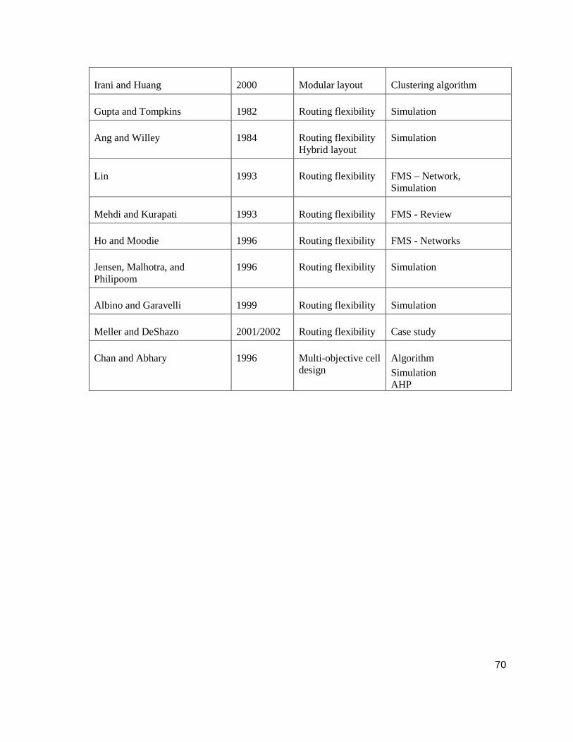
70

Irani and Huang 2000 Modular layout Clustering algorithm

Gupta and Tompkins 1982 Routing flexibility Simulation

Ang and Willey 1984 Routing flexibility

Hybrid layout

Simulation

Lin 1993 Routing flexibility FMS – Network,

Simulation

Mehdi and Kurapati 1993 Routing flexibility FMS - Review

Ho and Moodie 1996 Routing flexibility FMS - Networks

Jensen, Malhotra, and

Philipoom

1996 Routing flexibility Simulation

Albino and Garavelli 1999 Routing flexibility Simulation

Meller and DeShazo 2001/2002 Routing flexibility Case study

Chan and Abhary 1996 Multi-objective cell

design

Algorithm

Simulation

AHP

MULTIPERIOD PLANNING AND UNCERTAINTY ISSUES IN CELLULAR

Documents

Transcript of MULTIPERIOD PLANNING AND UNCERTAINTY ISSUES IN CELLULAR