ExxonMobil

Multiperiod Blend Scheduling ProblemMultiperiod Blend Scheduling Problem

Juan Pablo RuizIgnacio E. Grossmann

Department of Chemical EngineeringCenter for Advanced Process Decision-making

Carnegie Mellon UniversityCarnegie Mellon UniversityPittsburgh, PA 15213

Carnegie Mellon

1

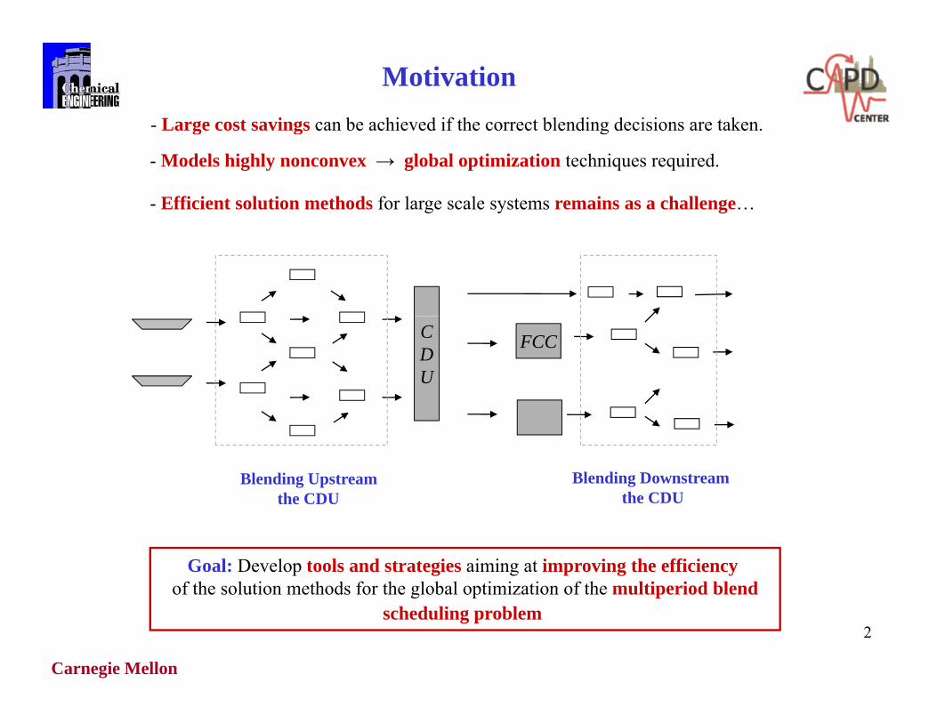
Motivation- Large cost savings can be achieved if the correct blending decisions are taken.g g g

- Models highly nonconvex → global optimization techniques required.

- Efficient solution methods for large scale systems remains as a challenge…

CDU

FCC

Blending Upstreamthe CDU

Blending Downstreamthe CDU

Goal: Develop tools and strategies aiming at improving the efficiencyof the solution methods for the global optimization of the multiperiod blend

the CDU the CDU

Carnegie Mellon

2

of the solution methods for the global optimization of the multiperiod blendscheduling problem

General Problem Topology

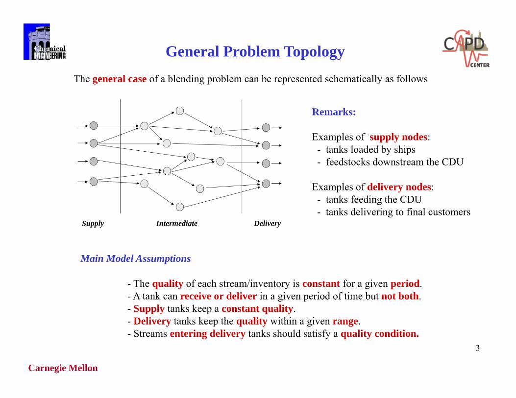
The general case of a blending problem can be represented schematically as follows

Remarks:

Examples of supply nodes: - tanks loaded by ships - feedstocks downstream the CDU

Supply Intermediate Delivery

Examples of delivery nodes: - tanks feeding the CDU - tanks delivering to final customers

Supply Intermediate Delivery

Main Model Assumptions

- The quality of each stream/inventory is constant for a given period.- A tank can receive or deliver in a given period of time but not both.- Supply tanks keep a constant quality.- Delivery tanks keep the quality within a given range.

Carnegie Mellon

3

y p q y g g- Streams entering delivery tanks should satisfy a quality condition.

Work lines - Summary

Alternative FormulationsAlternative Formulations

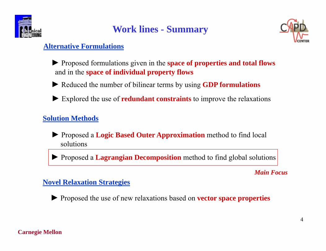
► Proposed formulations given in the space of properties and total flowsand in the space of individual property flows

► Reduced the number of bilinear terms by using GDP formulations

► Explored the use of redundant constraints to improve the relaxations

Solution Methods

► Proposed a Logic Based Outer Approximation method to find locall isolutions

► Proposed a Lagrangian Decomposition method to find global solutions

Main FocusNovel Relaxation Strategies

► Proposed the use of new relaxations based on vector space properties

Main Focus

Carnegie Mellon

4

AlternativeAlternative Formulations

Carnegie Mellon

5

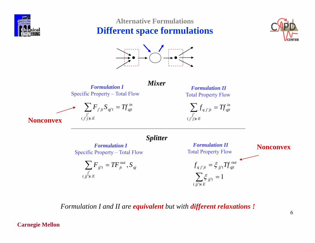
Alternative FormulationsDifferent space formulations

inTfSF

Mixer

inTff

Formulation ISpecific Property – Total Flow

Formulation IITotal Property Flow

qjt

Ejjj

tqjjtj TfSF )'(

'''

S litt

qjt

Ejjj

jtjq Tff )'(

''

Nonconvex

qjoutjttjj STFF ,'

Splitter

outqjttjjjtjq Tff ''

Formulation ISpecific Property – Total Flow

Formulation IITotal Property Flow

Nonconvex

qjjt

Ejjj

tjj ,)'('

Ejj

tjj

qjttjjjtjq ff

)'(' 1

Carnegie Mellon

6Formulation I and II are equivalent but with different relaxations !

Alternative Formulations

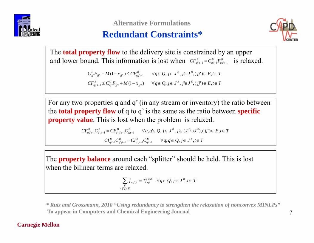
Redundant Constraints*

TtEjjJjJjQqCFxMFC DBBtqjjtjjtjj

Lqj ,)'(,',,)1( 1''''

The total property flow to the delivery site is constrained by an upperand lower bound. This information is lost when is relaxed.B

tqjjBqjt

Btqjj FCCF 1'11'

jjjjQqtqjjtjjtjjqj ,)(,,,)( 1

TtEjjJjJjQqxMFCCF DBtjjtjj

Uqj

Btqjj ,)'(,',,)1( '''1'

For any two properties q and q’ (in any stream or inventory) the ratio between

TtEjjJJjJjQqqCCFCCF BDBBqjt

Btjjq

Bjtq

Btqjj ,)'(),(',,',11''1'1'

y p p q q ( y y)the total property flow of q to q’ is the same as the ratio between specific property value. This is lost when the problem is relaxed.

TtJjQqqCCICCI BBqjt

Bjtq

Bjtq

Bqjt ,,',11'1'1

The property balance around each “splitter” should be held. This is lost when the bilinear terms are relaxed

TtJjQqTff Boutqjt

Ejjj

jtjq

,,)'('

'

when the bilinear terms are relaxed.

Carnegie Mellon

7* Ruiz and Grossmann, 2010 “Using redundancy to strengthen the relaxation of nonconvex MINLPs”To appear in Computers and Chemical Engineering Journal

Alternative Formulations

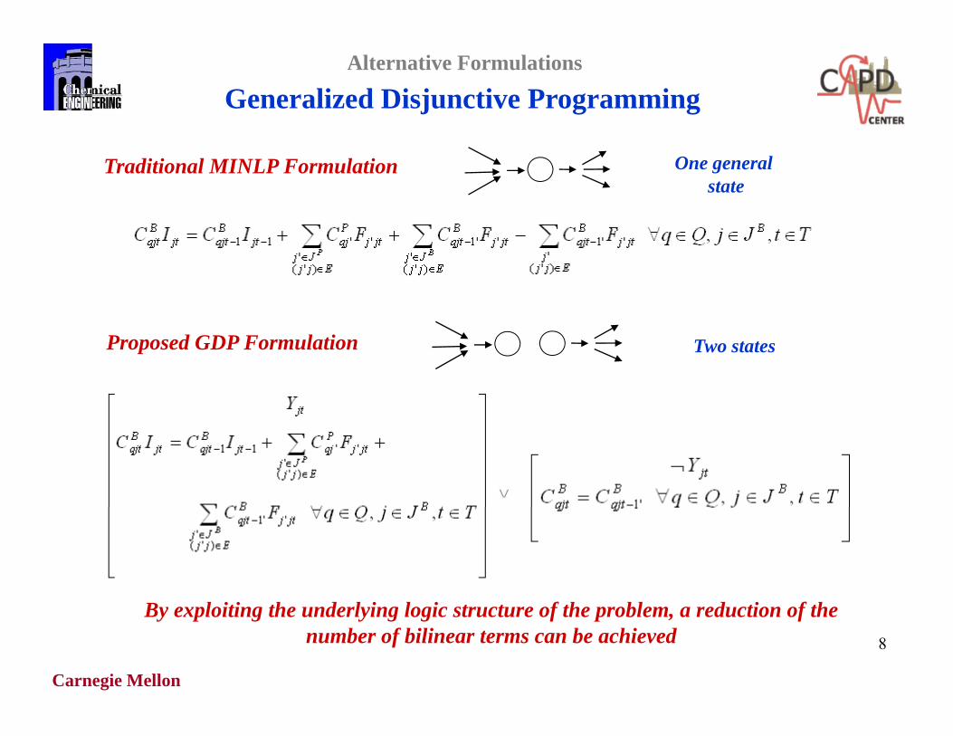
Generalized Disjunctive Programming

Traditional MINLP Formulation One general state

Proposed GDP Formulation Two states

Carnegie Mellon

8

By exploiting the underlying logic structure of the problem, a reduction of thenumber of bilinear terms can be achieved

S l ti M th dSolution Methods

Carnegie Mellon

9

Solution Methods

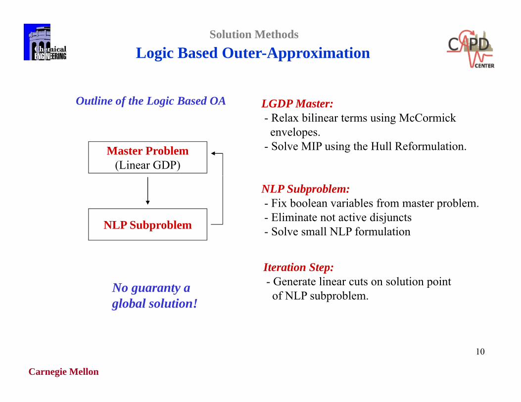
Logic Based Outer-Approximation

Outline of the Logic Based OA LGDP Master:- Relax bilinear terms using McCormick

Master Problem(Linear GDP)

envelopes. - Solve MIP using the Hull Reformulation.

NLP Subproblem

NLP Subproblem:- Fix boolean variables from master problem.- Eliminate not active disjuncts NLP Subproblem - Solve small NLP formulation

Iteration Step:li l i i- Generate linear cuts on solution point

of NLP subproblem.No guaranty a global solution!

Carnegie Mellon

10

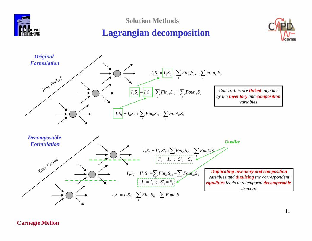
Lagrangian decompositionSolution Methods

iii SFoutSFinSISI 33332233

Original Formulation

i

ii

ii SFoutSFinSISI 22221122

i

ii

ii 33332233

Constraints are linked togetherby the inventory and composition

variables

i

ii

ii SFoutSFinSISI 11110011

D bl

i

ii

ii SFoutSFinSISI 33332233 ''

2222 ';' SSII

DualizeDecomposable Formulation

i

ii

ii SFoutSFinSISI 22221122 ''

iii SFoutSFinSISI 11110011

Duplicating inventory and compositionvariables and dualizing the correspondent

equalities leads to a temporal decomposablestructure

1111 ';' SSII

Carnegie Mellon

11

i

ii

ii 11110011

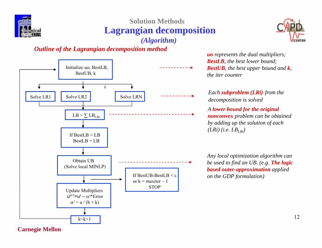
Lagrangian decomposition(Algorithm)

Solution Methods

Initialize uo, BestLB,BestUB, k

Outline of the Lagrangian decomposition methoduo represents the dual multipliers; BestLB, the best lower bound; BestUB, the best upper bound and k, the iter counter

Solve LR1 Solve LR2 Solve LRNEach subproblem (LRi) from the decomposition is solved

A lower bound for the originalLB = ∑ LBLRi

If BestLB < LBB tLB LB

A lower bound for the original nonconvex problem can be obtained by adding up the solution of each (LRi) (i.e. LBLRi)

BestLB = LB

Obtain UB(Solve local MINLP)

Any local optimization algorithm canbe used to find an UB. (e.g. The logic based outer-approximation applied

Update Multipliersut+1=ut – t*Errort = a / (b + k)

If BestUB-BestLB < or k = maxiter – 1

STOP

based outer approximation applied on the GDP formulation)

Carnegie Mellon

12

t = a / (b + k)

k=k+1

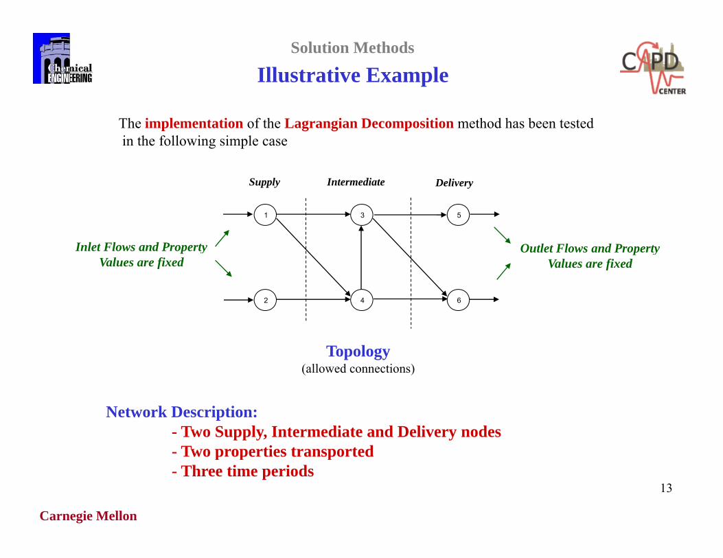
Illustrative ExampleSolution Methods

The implementation of the Lagrangian Decomposition method has been testedin the following simple case

3 51

Supply Intermediate Delivery

I l t Fl d P t O l Fl d P

42 6

Inlet Flows and PropertyValues are fixed

Outlet Flows and PropertyValues are fixed

Topology(allowed connections)

Network Description:- Two Supply, Intermediate and Delivery nodes- Two properties transported

Carnegie Mellon

13

Two properties transported- Three time periods

Lagrangian Decomposition

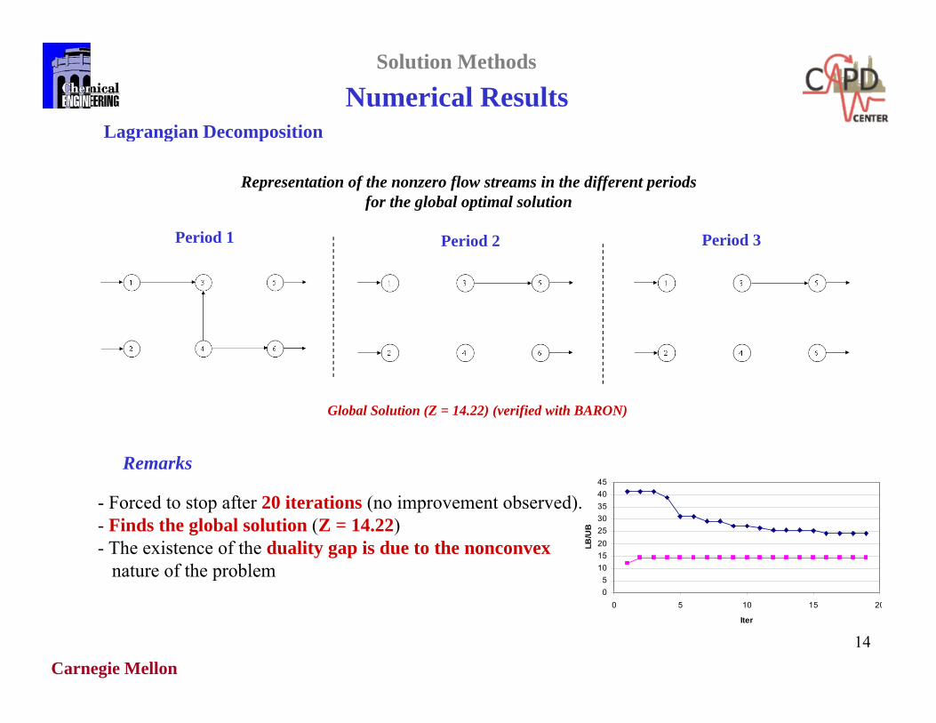
Numerical ResultsSolution Methods

Lagrangian Decomposition

Representation of the nonzero flow streams in the different periodsfor the global optimal solution

Period 1 Period 2 Period 3

Gl b l S l ti (Z 14 22) ( ifi d ith BARON)

F d t t ft 20 it ti ( i t b d) 4045

Global Solution (Z = 14.22) (verified with BARON)

Remarks

- Forced to stop after 20 iterations (no improvement observed). - Finds the global solution (Z = 14.22)- The existence of the duality gap is due to the nonconvex

nature of the problem 05

101520253035

LB/U

B

Carnegie Mellon14

00 5 10 15 20

Iter

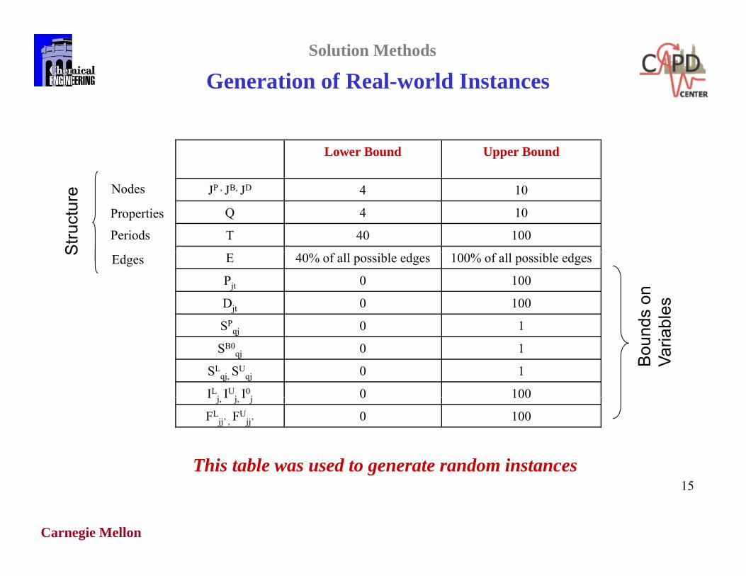
Generation of Real-world InstancesSolution Methods

Lower Bound Upper Bound

JP , JB, JD 4 10

Q 4 10

T 40 100

Nodes

Properties

Periods

Stru

ctur

e

E 40% of all possible edges 100% of all possible edges

Pjt 0 100

Djt 0 100

SP 0 1

EdgesS

ds o

nbl

es

SPqj 0 1

SB0qj 0 1

SLqj, SU

qj 0 1

ILj IU

j I0j 0 100

Bou

ndVa

riab

I j, I j, I j 0 100

FLjj’ , FU

jj’ 0 100

This table was used to generate random instances

Carnegie Mellon

15This table was used to generate random instances

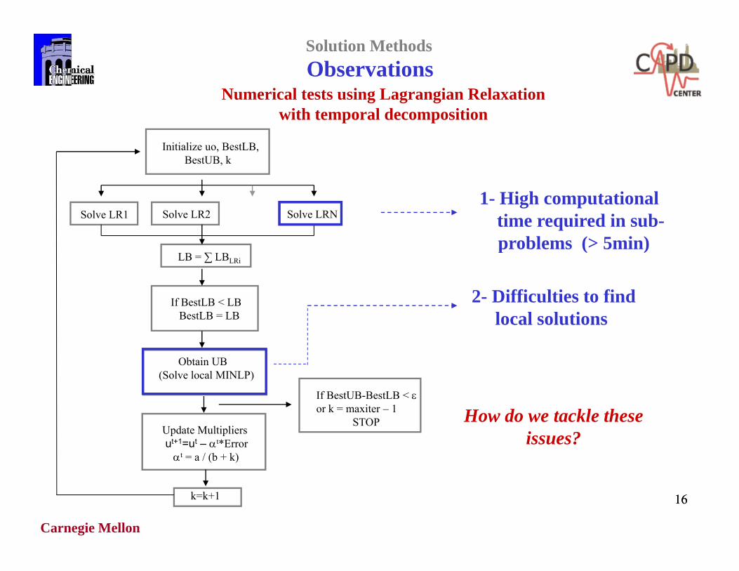
Numerical tests using Lagrangian RelaxationObservationsSolution Methods

with temporal decomposition

Initialize uo, BestLB,BestUB, k

Solve LR1 Solve LR2 Solve LRN1- High computational

time required in sub-problems (> 5min)

LB = ∑ LBLRi

If BestLB < LBBestLB = LB

p ( )

2- Difficulties to findlocal solutions

Obtain UB(Solve local MINLP)

If BestUB BestLB <

local solutions

Update Multipliersut+1=ut – t*Errort = a / (b + k)

If BestUB-BestLB < or k = maxiter – 1

STOP How do we tackle theseissues?

Carnegie Mellon

1616k=k+1

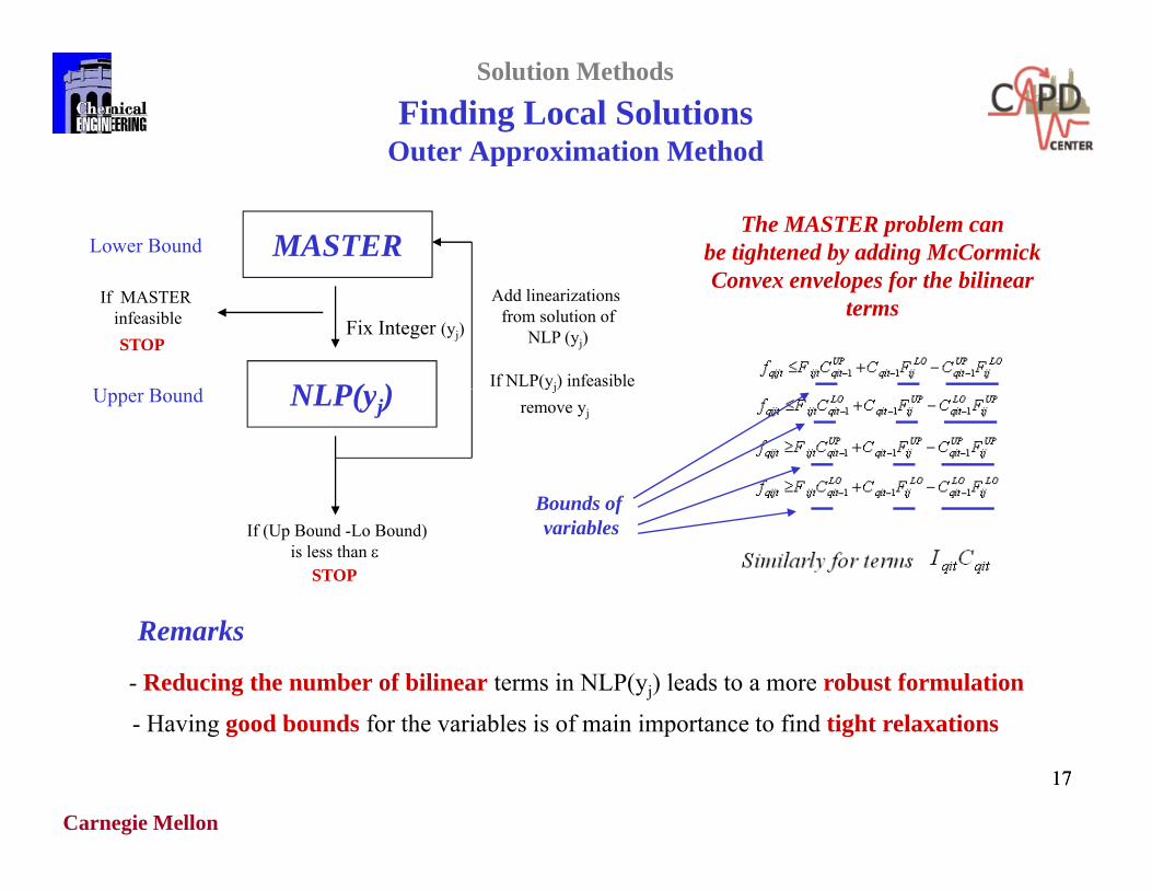
Finding Local SolutionsOuter Approximation Method

Solution Methods

pp

MASTERLower BoundThe MASTER problem can

be tightened by adding McCormickC l f th bili

NLP( )

Fix Integer (yj)

Add linearizations from solution of

NLP (yj)

U B d

If MASTER infeasibleSTOP

If NLP(yj) infeasible

Convex envelopes for the bilinearterms

NLP(yj)Upper Bound(yj)

remove yj

Bounds ofIf (Up Bound -Lo Bound)

is less than STOP

Bounds of variables

- Reducing the number of bilinear terms in NLP(yj) leads to a more robust formulation

Remarks

- Having good bounds for the variables is of main importance to find tight relaxations

Carnegie Mellon

1717

- Having good bounds for the variables is of main importance to find tight relaxations

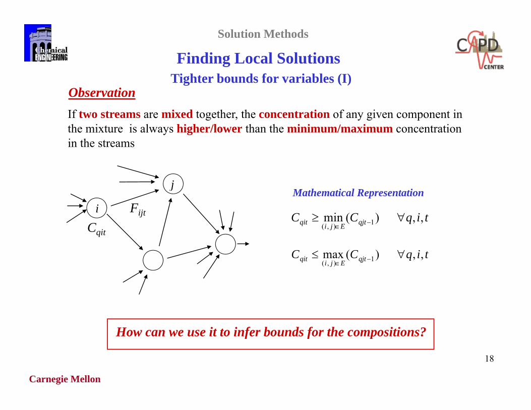
Finding Local SolutionsTi ht b d f i bl (I)

Solution Methods

ObservationIf two streams are mixed together, the concentration of any given component in the mixture is always higher/lower than the minimum/maximum concentration

Tighter bounds for variables (I)

the mixture is always higher/lower than the minimum/maximum concentration in the streams

i

j

Fijt

C ittiqCC qjtEjiqit ,,)(min 1),(

Mathematical Representation

Cqit

tiqCC qjtEjiqit ,,)(max 1),(

How can we use it to infer bounds for the compositions?

Carnegie Mellon

18

How can we use it to infer bounds for the compositions?

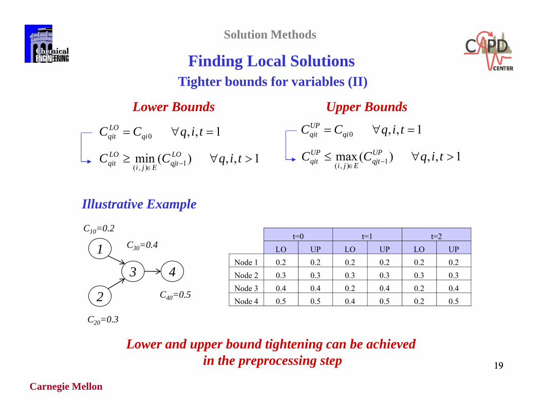
Finding Local SolutionsTi h b d f i bl (II)

Solution Methods

1 tiqCC LO 1 tiqCCUP

Lower Bounds Upper Bounds

Tighter bounds for variables (II)

1,,)(min 1),(

tiqCC LOqjtEji

LOqit

1,,0 tiqCC qiqit

1,,)(max 1),(

tiqCC UPqjtEji

UPqit

1,,0 tiqCC qiqit

Illustrative Example

t=0 t=1 t=2C10=0.2

1

3 4

t=0 t=1 t=2LO UP LO UP LO UP

Node 1 0.2 0.2 0.2 0.2 0.2 0.2Node 2 0.3 0.3 0.3 0.3 0.3 0.3Node 3 0 4 0 4 0 2 0 4 0 2 0 4

C30=0.4

2Node 3 0.4 0.4 0.2 0.4 0.2 0.4Node 4 0.5 0.5 0.4 0.5 0.2 0.5

L d b d ti ht i b hi d

C20=0.3

C40=0.5

Carnegie Mellon

1919

Lower and upper bound tightening can be achieved in the preprocessing step

Finding Local SolutionsTi ht b d f i bl (III)

Solution Methods

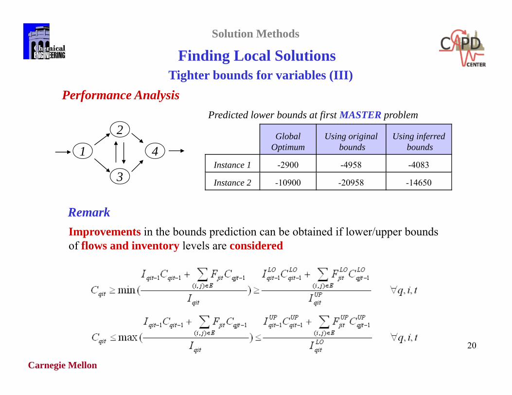
Tighter bounds for variables (III)Performance Analysis

Predicted lower bounds at first MASTER problem2

1 4

3

Global Optimum

Using originalbounds

Using inferredbounds

Instance 1 -2900 -4958 -40833 Instance 2 -10900 -20958 -14650

RemarkImprovements in the bounds prediction can be obtained if lower/upper bounds of flows and inventory levels are considered

Carnegie Mellon

20

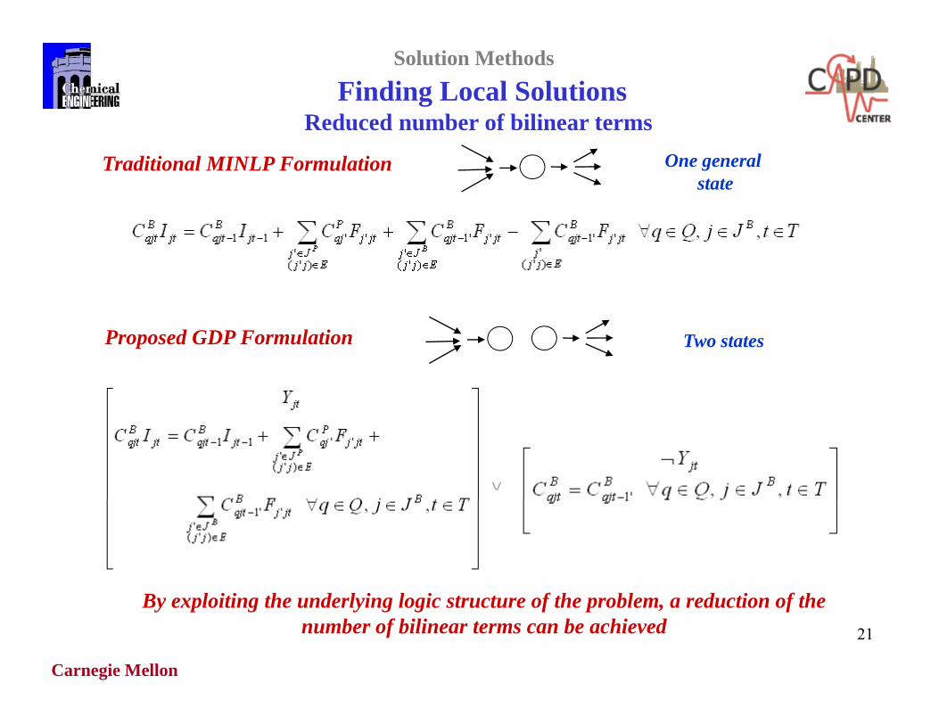
Finding Local SolutionsReduced number of bilinear terms

Solution Methods

Traditional MINLP Formulation One general state

Proposed GDP Formulation Two states

Carnegie Mellon

21

By exploiting the underlying logic structure of the problem, a reduction of thenumber of bilinear terms can be achieved

Finding Local Solutionsl

Solution Methods

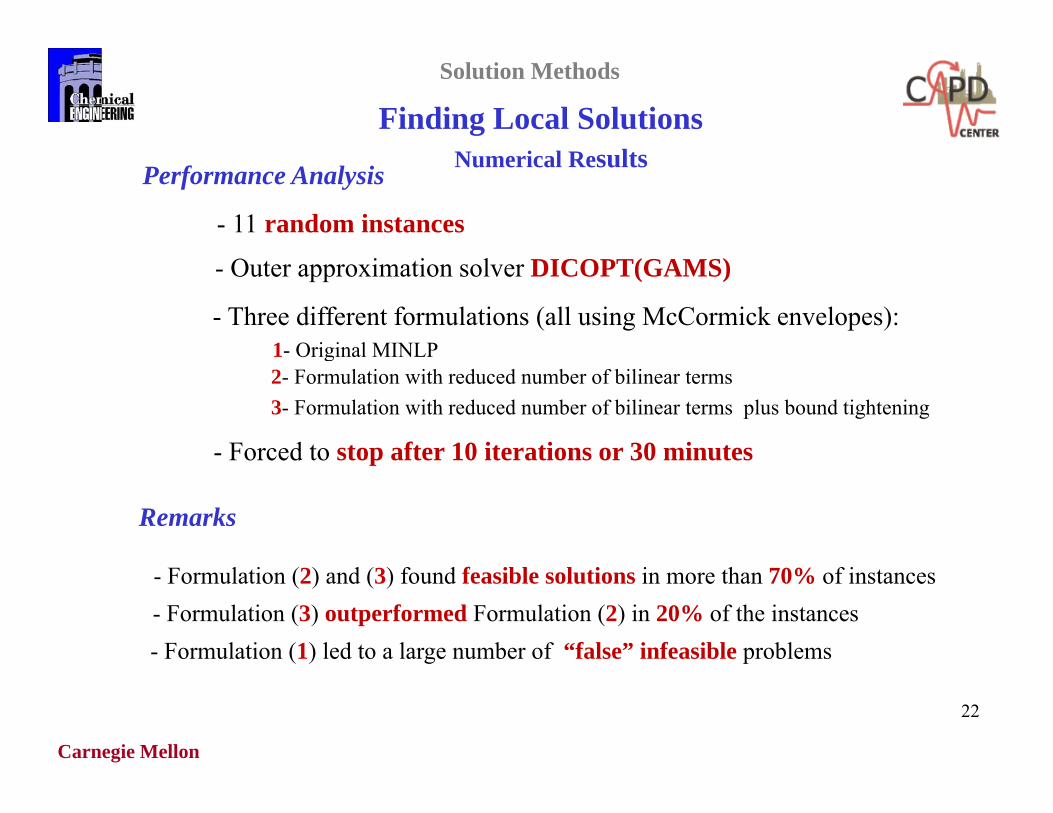
Numerical ResultsPerformance Analysis

- 11 random instances

- Outer approximation solver DICOPT(GAMS)

- Three different formulations (all using McCormick envelopes):1- Original MINLP1 Original MINLP 2- Formulation with reduced number of bilinear terms3- Formulation with reduced number of bilinear terms plus bound tightening

- Forced to stop after 10 iterations or 30 minutes

Remarks

Forced to stop after 10 iterations or 30 minutes

- Formulation (3) outperformed Formulation (2) in 20% of the instances - Formulation (1) led to a large number of “false” infeasible problems

- Formulation (2) and (3) found feasible solutions in more than 70% of instances

Carnegie Mellon

22

( ) g p

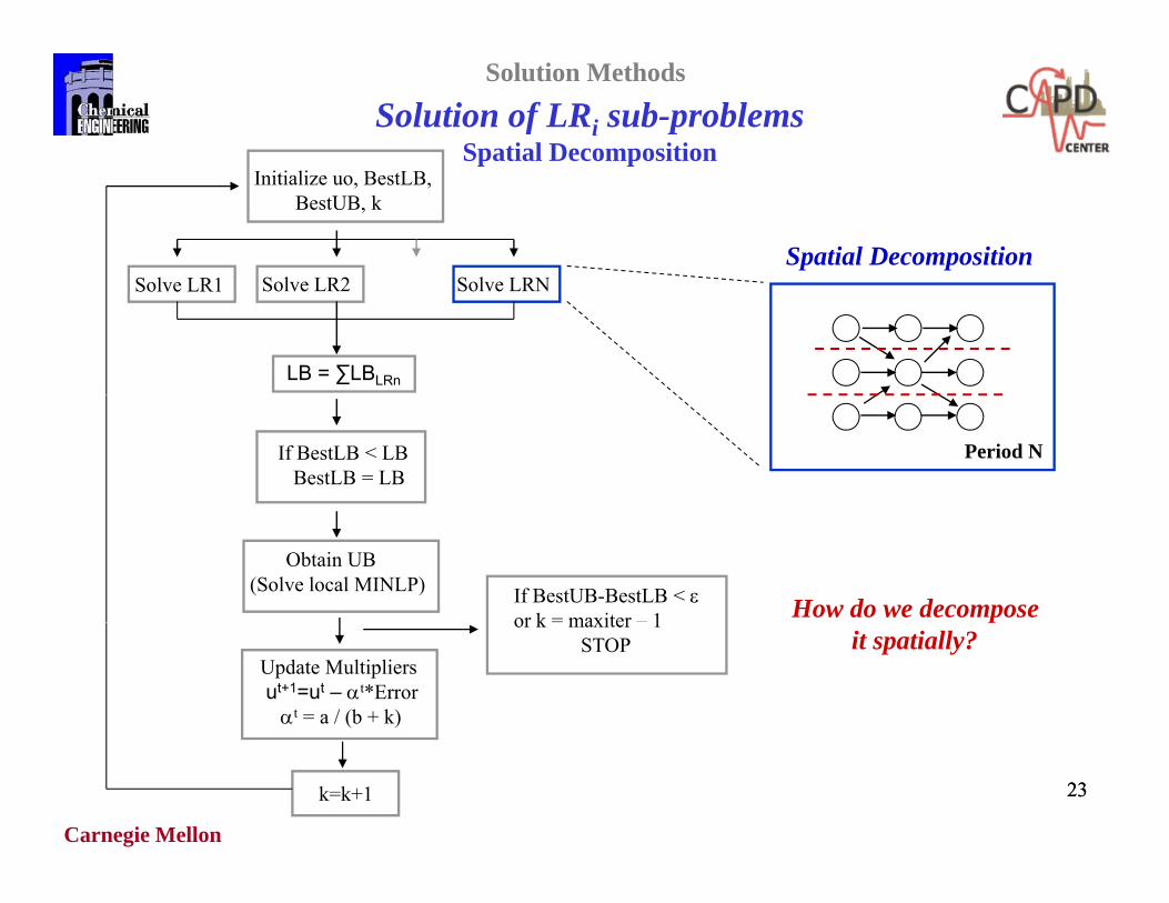
Solution of LRi sub-problemsSpatial Decomposition

Solution Methods

Initialize uo, BestLB,BestUB, k

S l LR1 S l LR2 S l LRNSpatial Decomposition

Solve LR1 Solve LR2 Solve LRN

LB = ∑LBLRn

If BestLB < LBBestLB = LB

Period N

Obtain UB(Solve local MINLP) If BestUB-BestLB <

or k = maxiter – 1 How do we decompose

Update Multipliersut+1=ut – t*Errort = a / (b + k)

or k maxiter 1 STOP

pit spatially?

Carnegie Mellon

2323k=k+1

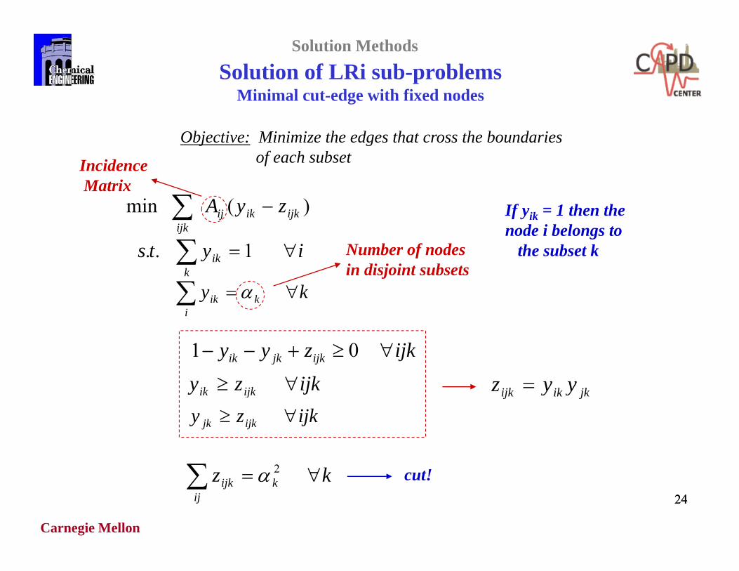
Solution of LRi sub-problemsMinimal cut-edge with fixed nodes

Solution Methods

Incidence

Objective: Minimize the edges that cross the boundariesof each subset

)(min ijkikijijk

zyA iyts 1 Number of nodes

MatrixIf yik = 1 then thenode i belongs to

the subset kiytsk

ik 1..

kyi

kik

Number of nodesin disjoint subsets

the subset k

ijkzyy ijkjkik 01ijkzy ijkik jkikijk yyz jy ijkik

ijkzy ijkjk

2

jkikijk yy

Carnegie Mellon

2424

kzij

kijk 2 cut!

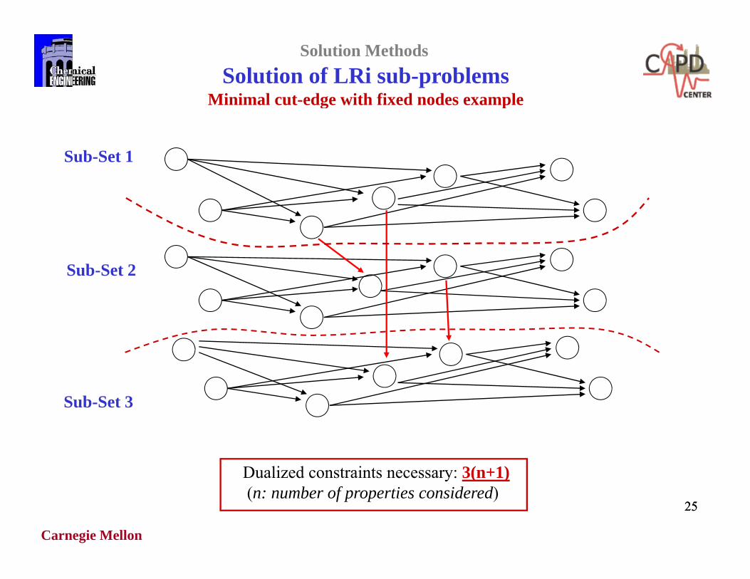
Solution of LRi sub-problemsMinimal cut-edge with fixed nodes example

Solution Methods

Sub-Set 1

g p

Sub-Set 2

S b S t 3Sub-Set 3

Dualized constraints necessary: 3(n+1)

Carnegie Mellon

2525

Dualized constraints necessary: 3(n+1)(n: number of properties considered)

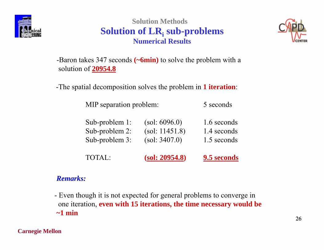
Solution of LRi sub-problemsNumerical Results

Solution Methods

-Baron takes 347 seconds (~6min) to solve the problem with a solution of 20954.8

-The spatial decomposition solves the problem in 1 iteration:

MIP separation problem: 5 seconds

Sub-problem 1: (sol: 6096.0) 1.6 secondsSub-problem 2: (sol: 11451.8) 1.4 secondsSub-problem 3: (sol: 3407 0) 1 5 secondsSub problem 3: (sol: 3407.0) 1.5 seconds

TOTAL: (sol: 20954.8) 9.5 seconds

Remarks:

- Even though it is not expected for general problems to converge inone iteration even with 15 iterations the time necessary would be

Carnegie Mellon

2626

one iteration, even with 15 iterations, the time necessary would be~1 min

NovelNovel Relaxations

Carnegie Mellon

27

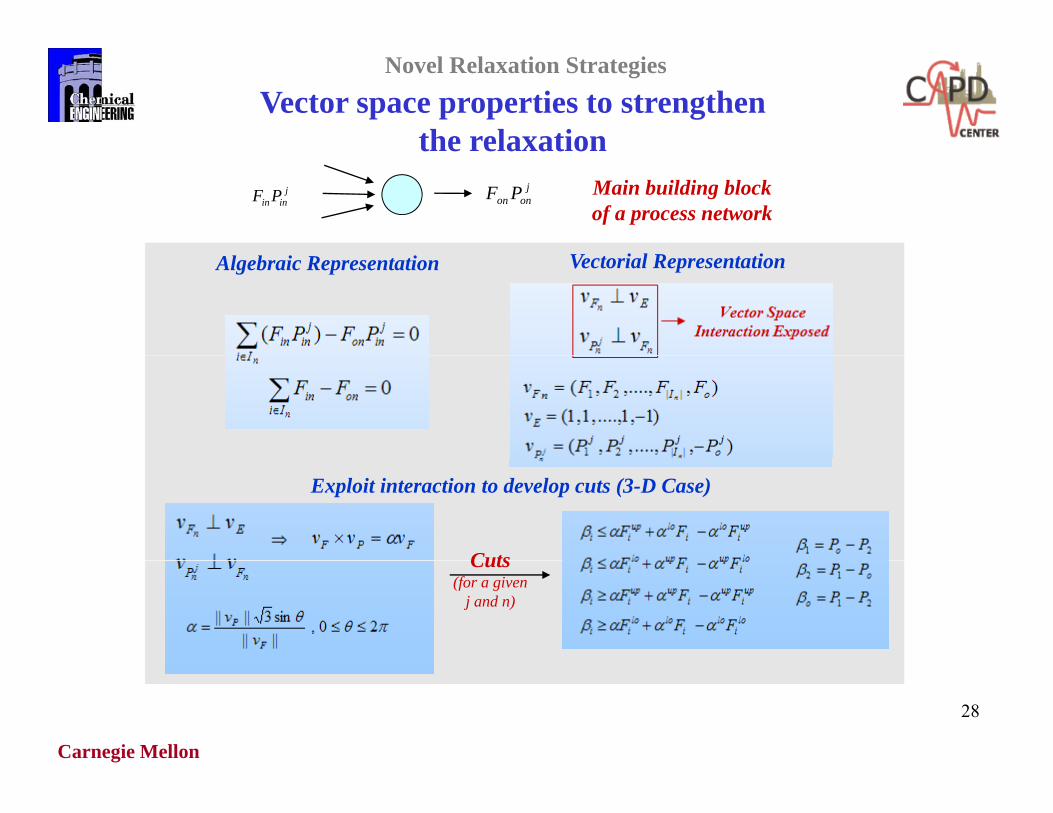
Vector space properties to strengthen the relaxation

Novel Relaxation Strategies

jinin PF j

onon PF Main building blockof a process network

the relaxation

Algebraic Representation Vectorial Representation

Exploit interaction to develop cuts (3-D Case)

CutsCuts(for a given

j and n)

Carnegie Mellon

28

Numerical Results*Novel Relaxation Strategies

Proposed ApproachTraditional Approach

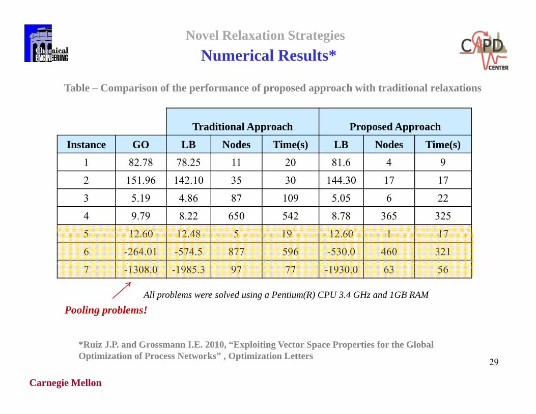
Table – Comparison of the performance of proposed approach with traditional relaxations

1717144 303035142 10151 962

9481.6201178.2582.781

Time(s)NodesLBTime(s)NodesLBGOInstance

Proposed ApproachTraditional Approach

17112 6019512 4812 605

3253658.785426508.229.794

2265.05109874.865.193

1717144.303035142.10151.962

17112.6019512.4812.605

321460-530.0596877-574.5-264.016

5663-1930.07797-1985.3-1308.07

All problems were solved using a Pentium(R) CPU 3.4 GHz and 1GB RAM

Pooling problems!

Carnegie Mellon

29

*Ruiz J.P. and Grossmann I.E. 2010, “Exploiting Vector Space Properties for the Global Optimization of Process Networks” , Optimization Letters

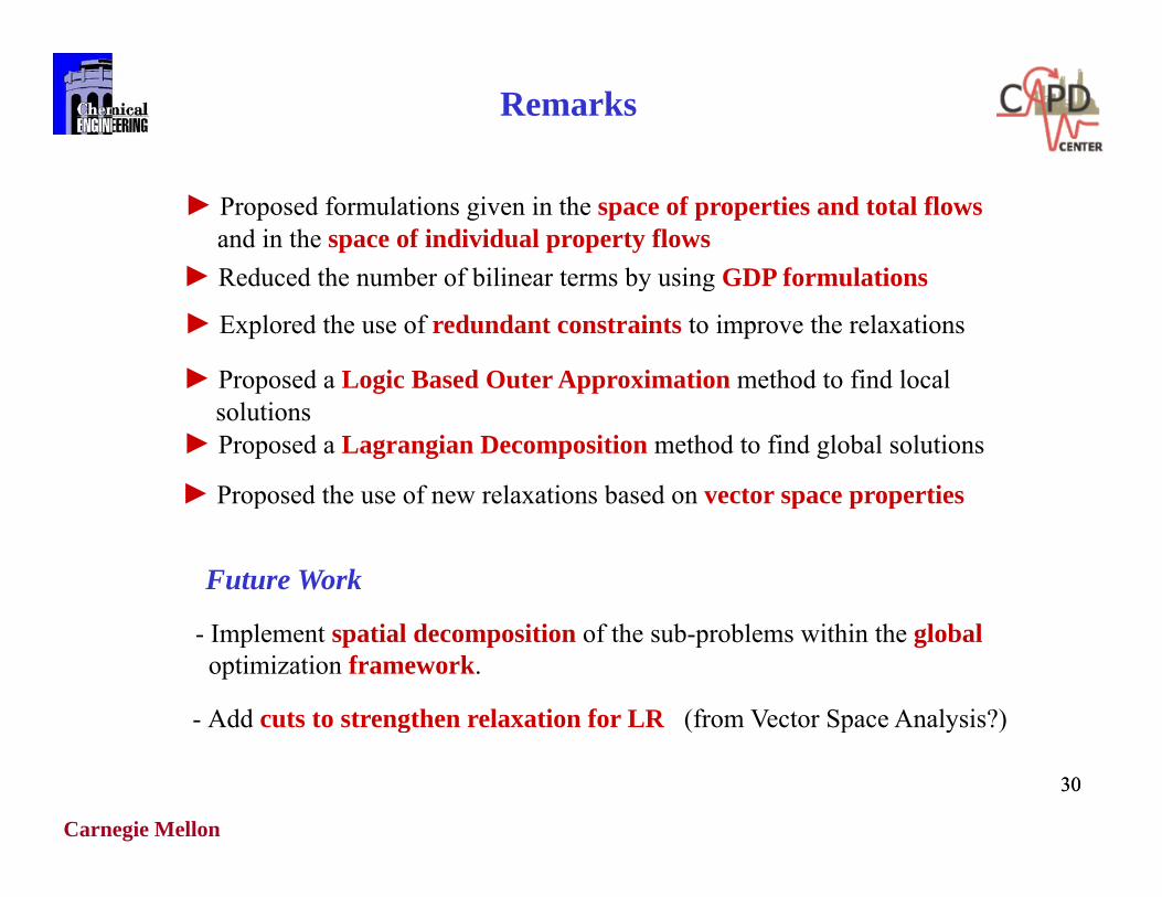
Remarks

► Proposed formulations given in the space of properties and total flowsand in the space of individual property flows

► Reduced the number of bilinear terms by using GDP formulations► Reduced the number of bilinear terms by using GDP formulations

► Proposed a Logic Based Outer Approximation method to find local

► Explored the use of redundant constraints to improve the relaxations

p g ppsolutions

► Proposed a Lagrangian Decomposition method to find global solutions

► Proposed the use of new relaxations based on vector space propertiesp p p p

Future Work

- Implement spatial decomposition of the sub-problems within the globaloptimization framework.

- Add cuts to strengthen relaxation for LR (from Vector Space Analysis?)

Carnegie Mellon

3030

g ( p y )