MULTILEVEL MODELING MULTILEVEL MODELING · PDF fileMULTILEVEL MODELING MULTILEVEL MODELING...

MULTILEVEL MODELING MULTILEVEL MODELING MULTILEVEL MODELING MULTILEVEL MODELING WORKSHOPWORKSHOPWORKSHOPWORKSHOP

APRIL 1, 2005APRIL 1, 2005APRIL 1, 2005APRIL 1, 2005

Presented by: Robert F. Dedrick, PhD John M. Ferron, PhD

Department of Measurement and Research

Sponsored by: College of Education

Contents of Workshop Packet

Content

Page

Purpose and Objectives 1

Slides Used in Workshop 2

Resource List 18

Key Figures in Multilevel Modeling 27

Software Examples—SAS 28

Software Examples—HLM6 31

Workshop Contributors 60

1

Multilevel Modeling Workshop

April 1, 2005 Overall Purpose of the Workshop: This workshop is designed to present an introduction to the uses and application of Multilevel Modeling in Educational Research and related fields. Objectives

� Present the logic behind Multilevel modeling

� Provide a description of the main types of Multilevel Modeling

� Introduce the general modeling approaches possible in Multilevel Modeling

� Discuss the advantages of Multilevel Modeling

� Present an overview of design issues to be considered when using Multilevel Modeling

� Describe the types of research questions and hypotheses that are appropriate to be answered through Multilevel Modeling

� Review approaches to the design of inquiry that use Multilevel Modeling

2

Slides Used in Workshop

Multilevel Modeling1. Overview

2. Application #1: Growth Modeling

Break

3. Application # 2: Individuals Nested Within Groups

4. Questions?

What is Multilevel or Hierarchical Linear Modeling?

Nested Data Structures

Overview

1. What is multilevel modeling?2. Examples of multilevel data structures3. Brief history4. Current applications5. Why multilevel modeling?6. What types of studies use multilevel

modeling?7. Computer Programs (HLM 6

SAS Mixed8. Resources

Several Types of Nesting

� 1. Individuals Nested Within Groups

Multilevel Question

� What effects do the following variables have on 3rd grade reading achievement?

School SizeClassroom ClimateStudent Gender

Individuals Undivided

Unit of Analysis = Individuals

3

Individuals Nested Within Groups

Unit of Analysis = Individuals + Classes

Examples of Multilevel Data Structures

� Schools are nested within districts

� Classes are nested within schools

� Students are nested within classes

… and Further Nested

Unit of Analysis = Individuals + Classes + Schools

Multilevel Data Structures

Level 4 District (l)

Level 3 School (k)

Level 2 Class (j)

Level 1 Student (i)

Examples of Multilevel Data Structures

� Neighborhoods are nested within communities

� Families are nested within neighborhoods

� Children are nested within families

2nd Type of Nesting

� Repeated Measures Nested Within Individuals

Focus = Change or Growth

4

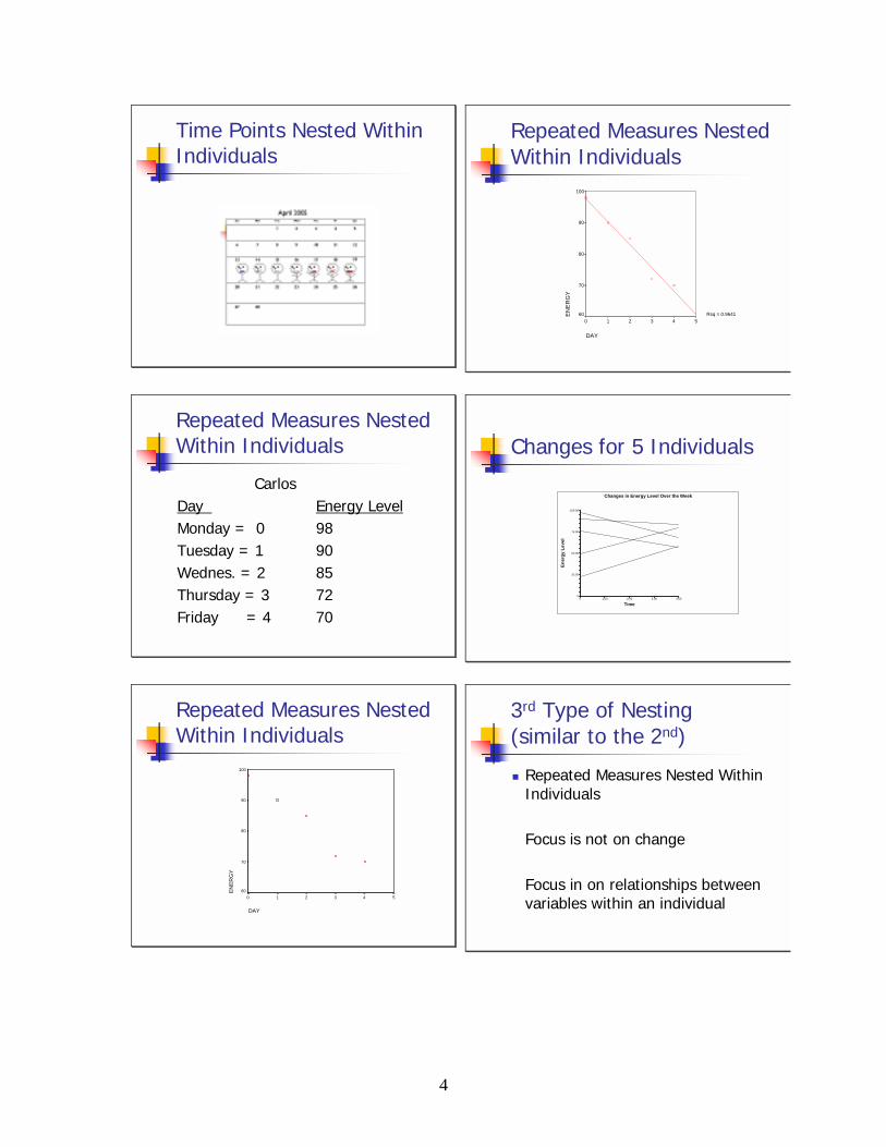
Time Points Nested Within Individuals

Repeated Measures Nested Within Individuals

DAY

543210

EN

ER

GY

100

90

80

70

60 Rsq = 0.9641


CarlosDay Energy LevelMonday = 0 98Tuesday = 1 90Wednes. = 2 85Thursday = 3 72Friday = 4 70

Changes for 5 Individuals

0 1.00 2.00 3.00 4.000

25.00

50.00

75.00

100.00

Time

Ener

gy L

evel

Changes in Energy Level Over the Week


DAY

543210

ENER

GY

100

90

80

70

60

3rd Type of Nesting (similar to the 2nd)

� Repeated Measures Nested Within Individuals

Focus is not on change

Focus in on relationships between variables within an individual

5


CarlosDay Hours of Sleep Energy LevelMonday 9 98Tuesday 8 90Wednesday 8 85Thursday 6 72Friday 7 70


2.00 4.50 7.00 9.50 12.000

25.00

50.00

75.00

100.00

Hours of Sleep

Ener

gy L

evel

Repeated Measures Nested Within Individuals (3 Individuals)

Repeated Measures Nested Within Individuals (Not Change)

HOURS

9.59.08.58.07.57.06.56.05.5

ENER

GY

100

90

80

70

60

Repeated Measures Within Persons

Level 2 Student (i)

Level 1 Repeated Measures Over Time (t)

Repeated Measures Nested Within Individuals (Not Change)

HOURS

9.59.08.58.07.57.06.56.05.5

ENER

GY

100

90

80

70

60

Nested Data

� Data nested within a group tend to be more alike than data from individuals selected at random.

� Nature of group dynamics will tend to exert an effect on individuals.

6

Nested Data

� Intraclass correlation (ICC) provides a measure of the clustering and dependence of the data

0 (very independent) to 1.0 (very dependent)

Details discussed later

Multilevel Articles

Frequency of Studies Employing HLM in Education or Related Journals

0

25

50

1999 2000 2001 2002 2003

Year

Freq

uenc

y

Total for 19 Journals ReviewedJournal of Personality and Social PsychologyChild Development Journal of Educational Research

Brief Historyof Multilevel Modeling

Robinson, W. S. (1950). Ecological correlations and the behavior of individuals. Sociological Review, 15, 351-357.

Burstein, Leigh (1976). The use of data from groups for inferences about individuals in educational research. Doctoral Dissertation, Stanford University.

Some Current Applications of Multilevel Modeling

� Growth Curve Analysis� Value Added Modeling of Teacher

and School Effects� Meta-Analysis

Table 1

Frequency of HLM application evidenced in Scholarly Journals

~1684939402020Total by Year

1112521Sociology of Education

101000Reading Research Quarterly

000000Journal of Research in Mathematics Education

000000Journal of Reading Behavior/Literacy Research

32135644Journal of Personality and Social Psychology

110000Journal of Experimental Education

000000Journal of Experimental Child Psychology

1353302Journal of Educational Research

1316321Journal of Educational Psychology

000000Journal of Educational Computing Research

300120Journal of Counseling Psychology

2067511Journal of Applied Psychology

000000Educational Technology, Research and Development

1222512Educational Evaluation and Policy Analysis

1775212Developmental Psychology

000000Contemporary Educational Psychology

100001Cognition and Instruction

29135623Child Development

~15?3453American Educational Research Journal

Total by journal20032002200120001999Journal

Multilevel Modeling Seems New But….

Extension of General Linear Modeling

Simple Linear RegressionMultiple Linear Regression

ANOVAANCOVA

Repeated Measures ANOVA

7

Multilevel Modeling

� Our focus will be on observed variables (not Latent Variables as in Structural Equation Modeling)

Problems withTraditional Approaches

1. Group level analysis (aggregate data and ignore individuals)

Aggregation bias = the meaning of a variable at Level-1 (e.g., individual level SES) may not be the same as the meaning at Level-2 (e.g., school level SES)

Why Multilevel Modelingvs. Traditional Approaches?

Traditional Approaches – 1-Level

1. Individual level analysis (ignore group)

2. Group level analysis (aggregate data and ignore individuals)

Multilevel Approach

� 2 or more levels can be considered simultaneously

� Can analyze within- and between-group variability

Problems withTraditional Approaches

1. Individual level analysis (ignore group)

Violation of independence of data assumption leading to misestimated standard errors (standard errors are smaller than they should be).

What Types of Studies Use Multilevel Modeling?

Quantitative

Experimental *Nonexperimental

(Survey, Observational)

8

How Many Levels Are Usually Examined?

2 or 3 levels very common

15 students x 10 classes x 10 schools= 1,500

HLM 6

Types of Outcomes

� Continuous Scale (Achievement, Attitudes)

� Binary (pass/fail)� Categorical with 3 + categories

Software to do Multilevel Modeling

SAS Users

Proc Mixed

Software to do Multilevel Modeling

SPSS Users2 SAV Files: Level 1

Level 2

HLM 6 (Menu Driven) (Raudenbush, Bryk, Cheong, & Congdon,

2004)

Resources (Sample…see handouts for more complete list)

� Books� Hierarchical Linear Models: Applications and

Data Analysis Methods, 2nd ed.Raudenbush & Bryk, 2002.

� Introducing Multilevel Modeling. Kreft & DeLeeum, 1998.

� Journals� Educational and Psychological Measurement� Journal of Educational and Behavioral

Sciences� Multilevel Modeling Newsletter

9

Resources (cont)(Sample…see handouts for more complete list)

� Software� HLM6� SAS (NLMIXED and PROC MIXED)� MLwiN

� Journal Articles� See Handouts for various methodological and

applied articles� Data Sets

� NAEP Data� NELS:88; High School and Beyond

Self-Check 2

� A researcher randomly selected 50 elementary schools and randomly selected 30 teachers within each school. The researcher was interested in the relationships between 2 predictors (school size and teachers’ years experience at their current school) and teachers’job satisfaction.

Self-Check 1

� A teacher with 1 classroom of 24 students used weekly curriculum-based measurements to monitor reading over a 14 week period. The teacher was interested in individual students’ rates of change and differences in change by male and female students.

Self-Check 2

� How would you classify this situation?

(a) not multilevel(b) 2-level(c) 3-level

Self-Check 1



Self-Check 3� 60 undergraduates from the research participant

pool volunteered for a study that used written vignettes to manipulate the interactional style (warm, not warm) of a professor interacting with a student. 30 randomly assigned students read the vignette depicting warmth and 30 randomly assigned students read the vignette depicting a lack of warmth. After reading the vignette students used a questionnaire to rate the likeability of the professor.

10

Self-Check 3



(Select ONLY one)

Research Questions

� What is an individual’s initial status on the outcome of interest?

Growth Curve Modeling

� Studying the growth in reading achievement over a two year period

� Studying changes in student attitudes over the middle school years

Run

Research Questions

� How much does an individual change during the course of the study?

Rise RisebRun

=

Research Questions

� What is the form of change for an individual during the study?

Research Questions

� What is the average initial status of the participants?

11

Research Questions

� What is the average change of the participants?

Research Questions

� To what extent does initial status relate to growth?

Research Questions

� To what extent do participants vary in their initial status?

Research Questions

� To what extent is initial status related to predictors of interest?

Research Questions

� To what extent do participants vary in their growth?

Research Questions

� To what extent is growth related to predictors of interest?

12

Design Issues

� How many waves a data collection are needed?� >2� Depends on complexity of growth curve

Design Issues

� How many participants are needed?

� More is better� Power analyses� > 30 rule of thumb

Design Issues

� Can there be different numbers of observations for different participants?

Examples� Missing data� Planned missingness

Design Issues

� How should participants be sampled?

� What you have learned about sampling still applies

Design Issues

� Can the time between observations vary from participant to participant?

Example: Students observed � 1, 3, 5, & 7 months� 1, 2, 4, & 8 months� 2, 4, 6, & 8 months

Design Issues

� What is the value of random assignment?

� What you have leaned about random assignment still applies

13

Design Issues

� How should the outcome be measured?

� What you have learned about measurement still applies

Example

� Level-1 model specification

β β= + +0 1 1* ( )fluencyY Time error

Example

� Context description

A researcher was interested in changes in verbal fluency of 4th grade students, and differences in the changes between boys and girls.

Example

� Level-2 model specification

ββ

= + +

= +0 00 01 2

1 10 11

* ( )* ( )

G G Gender errorG G Gender

ID Gender Time______

t0 t4 t7

1 0 20 30 302 0 40 44 493 0 45 40 604 0 50 55 595 0 42 48 536 1 45 52 617 1 39 55 638 1 46 58 689 1 44 49 59

Example

� Combined Model

= + + +

+ +00 01 10

11 2 1

* ( ) * ( )* ( ) * ( )

fluencyY G G Gender G TimeG Gender Time error error

14

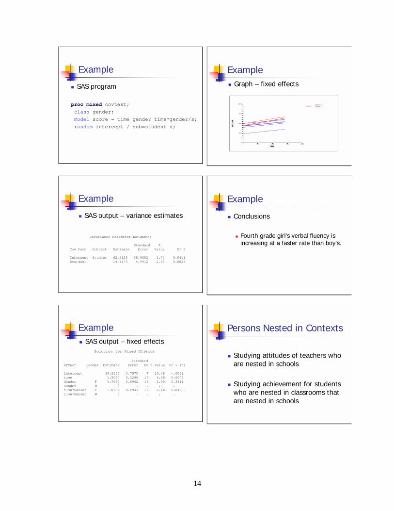
Example

� SAS program

proc mixed covtest;

class gender;

model score = time gender time*gender/s;

random intercept / sub=student s;

Example� Graph – fixed effects

0

25.00

50.00

75.00

100.00

SCO

RE

0 2.50 5.00 7.50 10.00

TIME

GENDER = 0GENDER = 1

Example

� SAS output – variance estimates

Covariance Parameter Estimates

Standard ZCov Parm Subject Estimate Error Value Pr Z

Intercept Student 62.5125 35.9682 1.74 0.0411Residual 14.1173 4.9912 2.83 0.0023

Example

� Conclusions

� Fourth grade girl’s verbal fluency is increasing at a faster rate than boy’s.

Example� SAS output – fixed effects

Solution for Fixed Effects

StandardEffect Gender Estimate Error DF t Value Pr > |t|

Intercept 39.8103 3.7975 7 10.48 <.0001time 1.5077 0.3295 16 4.58 0.0003Gender F 5.7090 5.6962 16 1.00 0.3311Gender M 0 . . . .time*Gender F 1.0692 0.4943 16 2.16 0.0460time*Gender M 0 . . . .

Persons Nested in Contexts

� Studying attitudes of teachers who are nested in schools

� Studying achievement for students who are nested in classrooms that are nested in schools

15

Research Questions

� How much variation occurs within and among groups?

� To what extent do teacher attitudes vary within schools?

� To what extent does the average teacher attitude vary among schools?

Research Questions

� To what extent is the relationship among selected within group factors and an outcome moderated by a between group factor?

� To what extent does the within schools relationship between student achievement and SES depend on the school adopted curriculum?

Research Questions

� What is the relationship among selected within group factors and an outcome?

� To what extent do teacher attitudes vary within schools as function of years experience?

� To what extent does student achievement vary within schools as a function of SES?

Design Issues

� Consider a design where students are nested in schools

� How should schools should be sampled?

� How should students be sampled within schools?

Research Questions

� What is the relationship among selected between group factors and an outcome?

� To what extent do teacher attitudes vary across schools as function of principal leadership style?

� To what extent does student math achievement vary across schools as a function of the school adopted curriculum?

Design Issues

� Consider a design where students are nested in schools

� How many schools should be sampled?

� How many students should be sampled per school?

16

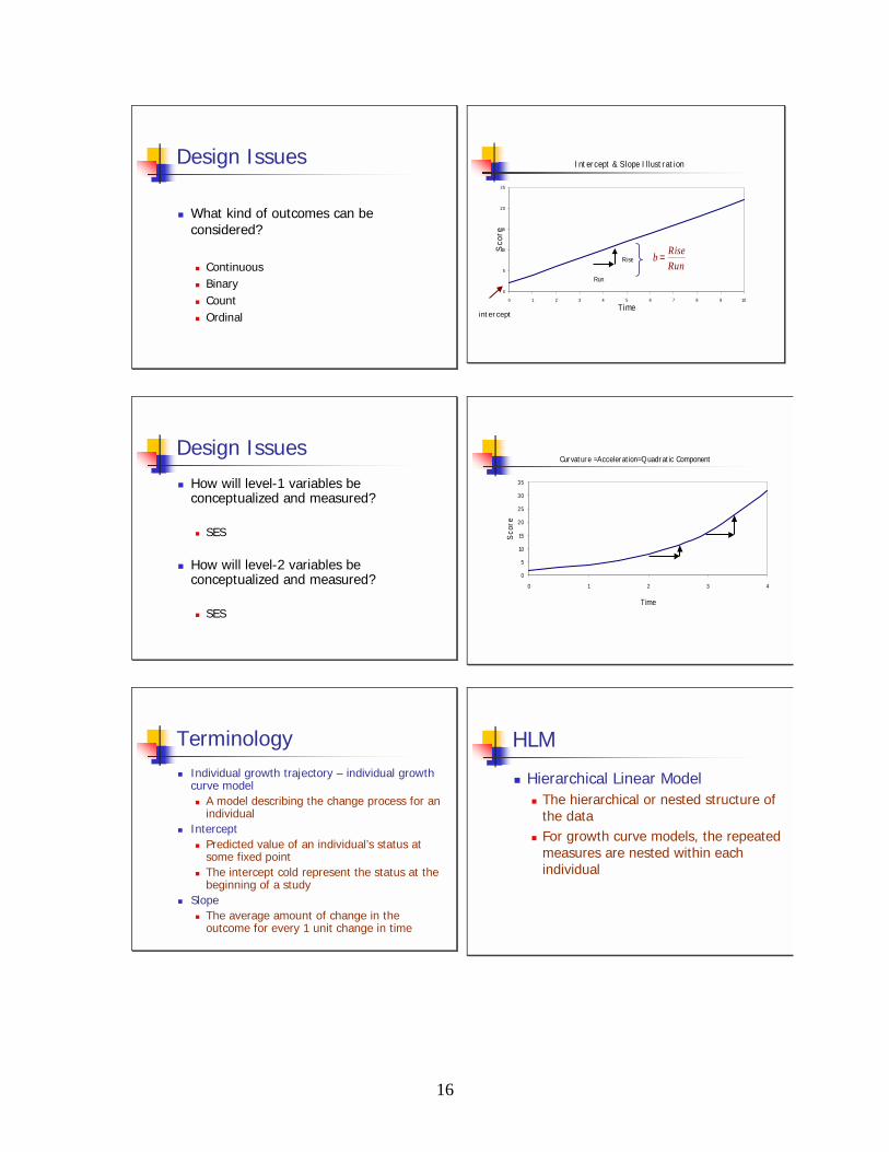
Design Issues

� What kind of outcomes can be considered?

� Continuous� Binary� Count� Ordinal

Intercept & Slope Illustration

0

5

10

15

20

25

0 1 2 3 4 5 6 7 8 9 10

Time

Sco

re

RiseRisebRun

=

Run

intercept

Design Issues

� How will level-1 variables be conceptualized and measured?

� SES

� How will level-2 variables be conceptualized and measured?

� SES

Curvature =Acceleration=Quadratic Component

0

5

10

15

20

25

30

35

0 1 2 3 4

Time

Scor

e

Terminology� Individual growth trajectory – individual growth

curve model� A model describing the change process for an

individual� Intercept

� Predicted value of an individual’s status at some fixed point

� The intercept cold represent the status at the beginning of a study

� Slope� The average amount of change in the

outcome for every 1 unit change in time

HLM

� Hierarchical Linear Model� The hierarchical or nested structure of

the data� For growth curve models, the repeated

measures are nested within each individual

17

Levels in Multilevel Models

� Level 1 = time-series data nested within an individual

0 1 *( )Y Time errorβ β= + +

More terminology� Balanced design

� Equal number of observations per unit� Unbalanced design

� Unequal number of observation per unit� Unconditional model

� Simplest level 2 model; no predictors of the level 1 parameters (e.g., intercept and slope)

� Conditional model� Level 2 model contains predictors of level 1

parameters

Levels in Multilevel Models

� Level 2 = model that attempts to explain the variation in the level 1 parameters

0 00 01

1 10 11

* ( )* ( )

G G Sessions errorG G Sessions error

ββ

= + +

= + +

Estimation Methods

� Empirical Bayes (EB) estimate� “optimal composite of an estimate

based on the data from that individual and an estimate based on data from other similar individuals” (Bryk, Raudenbush, & Condon, 1994, p.4)

More terminology

� Fixed coefficient� A regression coefficient that does not

vary across individuals

� Random coefficient� A regression coefficient that does vary

across individuals

Estimation Methods

� Expectation-maximization (EM) algorithm� An iterative numerical algorithm for

producing maximum likelihood esitmates of variance covariance components for unbalanced data.

18

Resource List

Books

Bryk, A., & Raudenbush, S.W. (1992). Hierarchical Linear Models for Social and Behavioral Research: Applications and Data Analysis Methods. Newbury Park, CA: Sage Publications.

Collins, L.M. & Horn, J.L. (Eds) (1991). Best Methods for the analysis of change. Washington, DC: American Psychological Association.

Hox, J. (2002). Multilevel Analysis: Techniques and Applications. Mahwah, N.J.: Lawrence Erlbaum Associates.

Kreft, I. & DeLeeum, J (1998). Introducting multilevel modeling. Newbury Park, CA: Sage Publications.

Raudenbush, S.W. & Bryk, A.S. (2002). Hierarchical Linear Models: Applications and Data Analysis Metods, 2nd Ed. Newbury Park, CA: Sage Publications.

Rogosa, D.R. & Saner, H. (1995). Questions and answers in the measurement of change. In E. Rothkopf (Ed.), Review of research in education (1988-89) (pp.345-422). Washingtonm DC: American Educational Research Associaiton.

Singer, J.D. & Willett, J.B. (2003). Applied Longitudinal Data Analysis: Modeling Change and Event Occurrence. Oxford University Press.

Skrondal, A. (2004). Generalized Latent Variable Modeling: Multilevel, Longitudinal, and Structural Equation Models. CRC Press.

Journals Journal of Educational and Behavioral Statistics

Multivariate Behavioral Research

Psychological Methods

Psychometrica

Sociological Methods and Research

Sociological Methodology

Articles General/Methodological Berkhof, J. & Snighder, T.A.B. (2001). Variance component testing in multilevel

models. Journal of Educational and Behavioral Statistics, 26, 133-152.

19

Bray, M. & Murray, T.R. (1995). Levels of comparison in educational studies: Different insights from different literatures and the value of multilevel analyses. Harvard Educational Review, 65, 472-490.

Bryk, A.S. & Raudenbush, S.W. (1987). Application of hierarchical linear models to assessing change, Psychological Bulletin, 101, 147-158.

Cohen, M. P. (1998). Determining sample sizes for surveys with data analyzed by hierarchical linear models. Journal of Official Statistics, 14, 267-275.

Ferron, J. (1997). Moving between hierarchical modeling notations. Journal of Educational and Behavioral Statistics, 119-123.

Francis, D.J., Fletcher, J.M., Stuebing, K.K., Davidson, K.C., & Thompsons, N.M. (1991). Analysis of change: Modeling individual growth. Journal of Consulting and Clinical Psychology, 59, 27-37.

Gibson, N.M. & Olejnik, S. (2003). Treatment of missing data at the second level of hierarchial linear models, Educational and Psychological Measurement. 63, 204-238.

Hedeker, D., & Gibbons, R.D. (1997). Application of random-effects pattern-mixture models for missing data in longitudinal studies. Psychological Methods, 2, 64-78.

Hill, P.W. & Goldstein, H. (1998). Multilevel modeling of educational data with cross-classification and missing identification for units, Journal of Educational and Behavioral Statistics, 23, 117-128.

Keselman, H.J., Algina, J., Kowalchuk, R.K., & Wolfinger, R.D. (1999). A comparison of recent approaches ot the analysis of repeated measurements. British Journal of Mathematical and Statistical Psychology, 52, 63-78.

Lawrence, F.R., & Hancock, G.R. (1998). Assessing change over time using latent growth modeling. Measurement and Evaluation in Counseling and Development, 30, 211-224.

MacCallum, R.C., Kim, C., Malarkey, W.B., & Kiecolt-Glaser, J.K. (1997). Studing multivariate change using multilevel models and latent curve analysis. Multivariate Behavioral Research, 32, 215-254.

Meredith, W. & Tisak, J. (1990). Latent curve analysis. Psychometrika, 55, 107-122.

Moerbeek, J., Breukelen, G.J.P., Berger, M.P.F. (2000). Design issues for experiments in multilevel populations, 25, 271-284.

Mok, M. (1995) Sample size requirements for 2-level designs in educational research. Multilevel Modeling Newsletter, 7, 11-15.

Morrell, C.H., Pearson, J.D., & Brant, L.J. (1997) Linear transformations of linear mixed-effects models. The American Statistician, 51(4), 338-343.

Osborne, J.W. (2001). Advantages of Hierarchial Linear Modeling. Practical Assessment, Research, & Evaluation, 7(1). (available at: http://pareonline.net/getvn.asp?v=7&n=1 )

20

Rasbash, J. & Goldstein, H. (1994). Efficient analysis of mixed hierarchical and cross-classified random structures using a multilevel model. Journal of Educational and Behavioral Statistics, 19, 337-350.

Rogosa, D.R. & Saner, H. (1995). Longitudinal data analysis examples with random coefficient models, Journal of Educational and Behavioral Statistics, 20, 149-170.

Singer, J.D. (1999). Using SAS PROC MIXED to fit multilevel models, hierarchila models, and individual growth models. Journal of Educational and Behavioral Statistics.

Snijders, T.A.B. & Bosker, R.J. (1993). Standard Error and sample sizes for two-level research. Journal of Educational Statistics, 18, 237-259.

Tate, R.L. & Wongbundhit, Y. (1983). Random versus nonrandom coefficient models for multilevel analysis. Journal of Educational Statistics, 8(2), 103-120.

Van Den Noortgate, W. & Onghena, P (2003). Multilevel Meta-Analysis: A comparison with traditional meta-analytical procedures. Educational and Pyuschological Measurement, 63 (765-790.

Willett, J.B., & Sayer, A.G. (1994). Using covariance structure analysis to detect correlates and predictors of individual change over time. Psychological Bulletin, 116, 363-381.

Willett, J.B., Singer, J.D., & Martin, N.C. (1998). The design and analysis of longitudinal studies of development and psychopathology in contest: Statistical models and methodological recommendations. Development and Psychopathology, 10, 395-426.

Woodhouse, G. Yang, M., Godstein, H., & Rasbash, J. (1996) Adjusting for measurement error in multilvevel analysis. Journal of Royal Statistical Society, 159 (2), 210-212.

Yann-yann,S. & Fouladi, R.T. (2003). The effect of multicollinearity on multilevel modeling parameter estimates and standard errors, Educational and Psychological Measurement, 63, 951-985.

Examples of Application in Educational Research Bradley, R. H., Corwyn, R. F., Burchinal, M., McAdoo, H. P., & Coll, C. G. (2001). The

home environments of children in the United States part II: Relations with behavioral development through age thirteen. Child Development, 72, 1868-1886.

Burchinal, M.R., Roberts, J.E., Riggins Jr., R.R., Zeisel, S.A., Neebe, E., and Bryant, D. (2000). Relating quality of center-based child care to early cognitive and language development longitudinally. Child Development, 71, 339-357.

21

Burns, R.B. and Mason, D.A. (2002). Class composition and student Achievement in elementary schools. American Educational Research Journal, 39, 207-233.

Dearing, E., McCartney, K., & Taylor, B. A. (2001). Change in family income-to-needs matters more for children with less. Child Development, 72, 1779-1793.

Greenhoot, A.F. (2000). Remembering and understanding: The effects of changes in underlying knowledge on children’s recollections. Child Development, 71, 1309-1328.

Hauser-Cram, P., Warfield, M. E., Shonkoff, J. P., Krauss, M. W., Upshur, C. C., & Sayer, A. (1999). Family influences on adaptive development in young children with down syndrome. Child Development, 70, 979-989.

Kochenderfer-Ladd, B., & Wardrop, J. L. (2001). Chronicity and instability of children’s peer victimization experiences as predictors of loneliness and social satisfaction trajectories. Child Development, 72, 134-151.

Lee, V.E. (2000). Using hierarchical linear modeling to study social contexts: The case of school effects. Educational Psychologist, 35, 125-141.

Ma, X. (2001). Bullying and being bullied: To what extent are bullies also victims? American Educational Research Journal, 38, 351-370.

Marsh, H.W., Koller, O., & Baumert, J. (2001). Reunification of East and West German school systems: Longitudinal multilevel modeling study of the Big-Fish-Little-Pond effect on academic self-concept. American Educational Research Journal, 38, 321-350.

Muller, C. and Schiller, K.S. (2000). Leveling the playing field? Students’ educational attainment and states’ performance testing. Sociology of Education, 73, 196-218.

NICHD Early Child Care Research Network, (2002). Early child care and children’s development prior to school entry: Results from the NICHD study of early child care. American Educational Research Journal, 39, 133-164.

Pituch, K.A. (2001). Using multilevel modeling in large-scale planned variation educational experiments: Improving understanding of intervention effects. The Journal of Experimental Education, 69, 347-372.

Roberts, J. E., Burchinal, M., & Durham, M. (1999). Parents’ report of vocabulary and grammatical development of African American preschoolers: Child and environmental associations. Child Development, 70, 92-106.

Rumberger, R.W. and Thomas, S.L. (2000). The distribution of Dropout and turnover rates among urban and suburban high schools. Sociology of Education, 73, 39-67.

Turner, J.C., Midgley, C., Meyer, D.K., Gheen, M., Anderman, E., Kang, Yongjin, & Patrick, H. (2002). The classroom environment and students’ reports of avoidance strategies in mathematics: A multimethod study. Journal of Educational Psychology, 94, 88-106.

Von Secker, C. (2002). Effects of inquiry-based teacher practices on science excellence and equity. Journal of Educational Research, 95, 3, 151-160.

22

Wang, J. (2000). Relevance of the hierarchical linear model to TIMSS data analyses. (Education (Chula Vista, Calif), 120, 787-789.

Wilkings, J. L. M., & Ma, X. (2002). Predicting student growth in mathematical content knowledge. Journal of Educational Research, 95, 5, 288-298.

Websites

Missing Data http://www.missingdata.org.uk

Teaching Resources and Materials for Social Scientists http://tramss.data-archive.ac.uk

Multilevel Modeling Resources at UCLA Academic Technology Services http://www.ats.ucla.edu/stat/mlm/default.htm

Resources to help you learn and use MLwiN at UCLA Academic Technology Services http://www.ats.ucla.edu/stat/mlwin/default.htm

UCLA MLwiN portal at UCLA Academic Technology Services http://statcomp.ats.ucla.edu/mlwin

www.scholar.google.com This is the beta version of the google scholar search engine. The following keywords (and derivations thereof) may be used to assist in searching this engine as well as libraries and other search engines:

- Multilevel Modeling

- Hierarchical Linear Model (s) (ing)

- Growth Curve Analysis

- Mixed Models

Software GLLAMM (for more information go to: http://www.gllamm.org/install.html)

HLM6 (free student version download at: http://www.ssicentral.com/other/hlmstu.htm)

NOTE: Other helpful links as well for multilevel modeling resources MLwiN (for more information go to: http://multilevel.ioe.ac.uk/features/index.html )

NOTE: Other helpful links as well for multilevel modeling resources SAS PROC MIXED (SAS Institute, for more information, go to: www.sas.com)

SAS PROC NLMIXED (SAS Institute, for more information, go to: www.sas.com)

23

Data Sets The following website has 11 different data sets available for download for learning and using multilevel modeling techniques. Achknowledgement information is contained on the website.

http://multilevel.ioe.ac.uk/intro/datasets.html

Multilevel Modelling Newsletter The Multilevel Modelling Newsletter is generally published twice yearly. Please send any comments to the Editor, Ian Plewis. To subscribe to the newsletter and have copies sent directly to your e-mail address, e-mail Amy Burch requesting newsletter subscription. Please supply your e-mail address, name and postal address.

Sample titles of articles appearing in the Multilevel Modelling Newsletter

Retrieved from the website: http://multilevel.ioe.ac.uk/publref/newsletters.html

Volume/No.��

� Title of Article��

� Authors��

�

The Role of the Hausman Test and whether Higher Level Effects should be treated as Random or Fixed�

A. Fielding�Volume 16 No. 2 December 2004� Multiple Imputation using MLwiN� J. Carpenter and H.

Goldstein�

Volume 15 No. 2 December 2003�

Bootstrapping the Effects of Measurement Errors� D. Hutchison�

Volume 15 No. 1 September 2003�

Some Design Problems with Multilevel Data� T. Lewis�

Modelling ordinal data using MLwiN� I. Plewis�Volume 14 No. 1 July 2002� Fitting multilevel models under

informative probability sampling�D. Pfefferman, F. Moura and P. Nascimento Silva�

Volume 13 No. 2 December

The effect on variance component estimates of ignoring a level in a multilevel model�

D. Hutchison and M. Healy�

24

2001� A non-parametric random coefficient approach: the latent class regression model�

J. K. Vermunt and L. A. van Dijk�


Using ordinal multilevel models to assess the comparability of examinations�

J. F. Bell & T. Dexter�

A Non-parametric bootstrap for multilevel models�

J. Carpenter, H. Goldstein & J. Rasbash�

Random effects meta-analysis of trials with binary outcomes using multilevel models in MLwiN�

R. Turner, R. Z. Omar, M. Yang, H. Goldstein & S. G. Thompson�


Standard errors in multilevel analysis� N. Longford�

Fitting multilevel models using SAS PROC MIXED�

J. D. Singer�

Multilevel Modeling in Windows; a review of MLwiN�

J. Hox�

Volume 10 No. 2 November 1998�

Numerical integration via High-Order, Multivariate LaPlace Approximation with Application to Multilevel Models�

S. W. Raudenbush & M. Yang�

Multilevel models where the random effects are correlated with the fixed predictors: a conditioned iterative generalised least squares estimator (CIGLS)�

N. Rice, A. Jones & H. Goldstein �

Volume 10 No. 1 February 1998�

Random effects for event data - evaluating effectiveness of universities through the analysis of student careers�

E. Gori & M. Montagni�


Using MLn for repeated measures with missing data�

T. A. B. Snijders & C. J. M. Maas�

Consistent estimators for multilevel generalised linear models using an iterated bootstrap�

H. Goldstein�Volume 8 No. 1 April 1996�

Multilevel models for longitudinal growth norms�

H. Pan, H. Goldstein & J. Rasbash�

25

Multilevel Unit Specific and Population Average Generalised Linear Models�

H. Goldstein�

The Effects of Centering in multilevel Analysis : is the public school the loser or the winner? A new Analysis of an Old Question�

I. Kreft�


The Use of Multilevel Models for Screening Data Accumulated from Number of Studies�

V. Simonite�

Detecting Outliers in Multilevel Models: an overview�

I. Langford & T. Lewis�

Implementing the Bootstrap Multilevel Models�

E. Meijer, R. Leeden & F. M. T. A. Busing�

Sample Size Requirements for 2-Level Designs in Educational Research�

M. Mok�

Volume 7 No. 2 June 1995�

Meta-Analysis Using Multilevel Models� P. Lambert & K. Abrams�

A Crossed Random Effects Model for Studying Social Context Effects on Individual Growth�

S. W. Raudenbush�

Explained variance in Two-level Models� T. Snijders & R. Bosker�

Improved Estimation for Logit and Loglinear Multilevel Models�

H. Goldstein�

Modelling the Accuracy and Precision of Portable Peak Exploratory Flow Meters�

P. Burton�

Multilevel Logistic Regression Models in Educational Research: GCSE Estimated Grades�

M. R. Delap�

Random-Effects Regression Models a) with Autocorrelated Errors and b) for Ordinal Outcomes�

D. Hedeker & R. Gibbons�

Volume 6 No. 1 March 1994�

Using Multilevel Multinomial Regression to Analyse Line-up Data�

D. Wright & A. Sparks�

26

A Three Level Growth Model for Educational Achievement: effects of holidays, social-economic background and absenteeism�

H. Bergh & K. Kuhlemeier�Volume 4 No. 2 June 1992�

Multilevel Models for Comparing Schools� H. Goldstein et al�

Volume 4 No. 1 January 1992�

Multilevel Modelling and Segregation Indices�

L. Paterson�

Health Information Research Services and Multilevel Models�

K. Jones & G. Moon�Volume 3 No. 1 October 1991�

New Statistical Methods for Analysis Social Structures: an introduction to multilevel models�

L. Paterson & H. Goldstein�

Examining Missingness in Hierarchically Structured Data with a Multilevel Logistic Regression Model�

R. Prosser�

Grafted Polynomials Useful for Cross-Sectional Growth Analysis�

H. Q. Pan, H. Goldstein & R. Prosser�

Volume 2 No. 3 November 1990�

Multilevel Covariance Structure Work� B. Muthén�

Volume 2 No. 2 June 1990�

Multilevel Models with Known Level 1 Variance Structures�

S. W. Raudenbush�

Fitting Log-linear ML Models� H. Goldstein�Volume 2 No. 1 January 1990� Multilevel Models for Data with a Non-

normal Distribution�N. Longford�

A Response to Longford & Plewis� S. W. Raudenbush�

Comment on ‘Centering’ Predictors in Multilevel Analysis�

I. Plewis�

Contextual Effects and Group Means� N. Longford�

Multilevel Models Useful for Examining Interviewer Effects in Surveys�

R. Wiggins, C. O’Muircheartaigh & N. Longford�

Volume 1 No. 3 October 1989�

To Center or Not to Center� N. Longford�

27

Key Figures in Multilevel Modeling

Author Year of Degree

University Title of Dissertation

Burstein, Leigh 1976 Stanford The use of data from groups for

inferences about individuals in educational research

Bryk, Anthony S. 1977 Harvard An investigation of the effectiveness of

alternative statistical adjustment strategies in the analysis of quasi-experimental growth data.

Willms, Jon Douglas

1983 Stanford Achievement outcomes in public and private high schools

Singer, Judith Donna

1983 Harvard An intraclass correlation approach to modeling the effects of group composition on individual outcomes in studies of hierarchical data (unit-of-analysis, multi-level)

Raudenbush, Stephen Webb

1984 Harvard Applications of a hierarchical linear model in educational research

Willett, John Barry 1985 Stanford Investigating systematic individual

differences in academic growth (change, correlates)

28

EXAMPLES

SAS Example SAS Code for Nested Model

title1 'Exanoke SAS Code for Nested Model;proc format;value ifmt 1='Programmed Inst' 2='CAI';

data one;input instruct 1 teacher $ 3-7 Student 10-11 Score 19-20;label instruct='Type of Instruction'

teacher='Individual Teacher';format instruct ifmt.;

cards;1 Jones 1 91 Jones 2 71 Jones 3 101 Jones 4 81 Smith 5 101 Smith 6 141 Smith 7 81 Smith 8 121 Wills 9 81 Wills 10 31 Wills 11 31 Wills 12 72 Benny 13 122 Benny 14 142 Benny 15 102 Benny 16 142 Wundt 17 112 Wundt 18 132 Wundt 19 92 Wundt 20 92 Lunnt 21 142 Lunnt 22 102 Lunnt 23 92 Lunnt 24 14;proc glm; class instruct;model score = instruct;means instruct;title2 'Analysis of Individual Scores: Student as Unit of Analysis';

proc glm; class instruct teacher;model score = instruct teacher(instruct);test h=instruct e=teacher(instruct);means instruct;title2 'Hierarchical Analysis';

* +-----------------------------------------+Use proc means to obtain the mean scorefor each class of students. Then conductANOVA on class means.

+-----------------------------------------+;

29

proc sort data=one;by instruct teacher;

proc means noprint data=one;by instruct teacher;var score;output out=q mean=mnscore;

proc glm; class instruct;model mnscore = instruct;means instruct;title2 'Analysis of Class Means';

run;proc mixed data=one noclprint covtest;class instruct teacher;model score = / s;random intercept / sub=teacher s;title2 'Baseline Model';

run;proc mixed data=one noclprint covtest;class instruct teacher;model score = instruct / s;random intercept / sub=teacher(instruct) s;title2 'Multilevel Model';

run;

Example SAS Code for Growth Curve Model

Data one;Input Student Gender $ September November April;

Cards;1 M 20 30 302 M 40 44 493 M 45 40 604 M 50 55 595 M 42 48 536 F 45 52 617 F 39 55 638 F 46 58 689 F 44 49 59;proc glm;class gender;model September November april = gender / nouni;repeated time 3;title ' Example SAS Code for Longitudinal Data’;

data two;set one;

array meas[3] September November april;do time = 1 to 3;score = meas[time];output;

end;data three;set two;

if time = 1 then time = 0;if time = 3 then time = 7;

30

proc mixed data=three noclprint covtest;class gender;model score = time / s;random intercept / sub=student s;title 'Baseline Model';

run;proc mixed data=three noclprint covtest;class gender;model score = time gender time*gender / s;random intercept / sub=student s;title 'Growth Curves';

run;

31

HLM6

Growth Curve Example in LM6

Level 1 File (Measures Within Persons)Each person was measured 3 times at 0, 2 and 7 months. The data needto be arranged so that each person has a unique ID and each score forthe separate time points is on a separate line. Although everyone inthis dataset had 3 scores measured at exactly the same 3 times, this isnot necessary. If someone was measured at 0, 3, and 8, these would bethe 3 numbers that would be input under the Time column for thisindividual. If someone was measured at 2 time points (2 and 7 months)that person would only have 2 lines of data.

The ID is important because it is used to link the Level 1 File withthe Level 2 file.

ID Time Score1 0 201 2 301 7 302 0 402 2 442 7 493 0 453 2 403 7 604 0 504 2 554 7 595 0 425 2 485 7 536 0 456 2 526 7 617 0 397 2 557 7 638 0 468 2 588 7 689 0 449 2 499 7 59

Level 2 File (Person Data)ID Gender (0=Male, 1=Female)1 02 03 04 05 06 17 18 19 1

32

HLM 6 Screen Shots

HLM 6 Menu Driven Program

(Raudenbush, S., Bryk, A., Cheong, Y. F., & Congdon, R., 2004)

If you are an SPSS user, you would, prior to entering the HLM 6 Program, have your Level 1 SAV file and Level 2 SAV file created.

33

To run HLM Models you need to create an MDM file (multivariate data matrix). Assume you are an SPSS user and you have created your Level 1 SAV file and your Level 2 SAV file (2 files are needed even though you may have all of the information in one file). Stat Package Input will allow you to select SPSS as an option for input.

34

Click HLM2 to do a 2 Level Model There are 2 types of 2 level models: persons within groups measures within persons

35

The Browse buttons allow you to locate your SPSS Level 1 SAV file and your SPSS Level 2 SAV file

36

A name has to be inserted in the MDM File box (this MDM file will be used for any future models you would run – you don’t have to go through all the previous steps every time you want to run HLM).

37

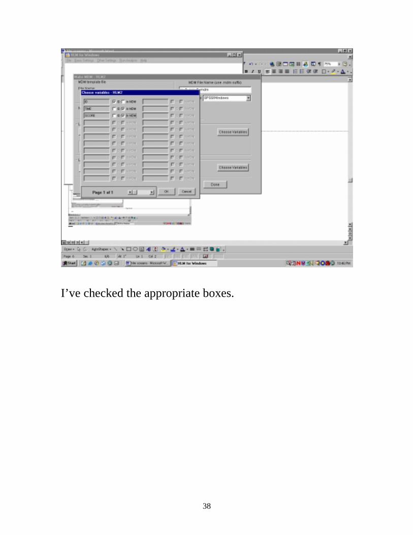
This screen lists all of the variables that are coming from your SPSS Level 1 SAV file. Sometimes you don’t want to analyze all of your variables so here is the place you can check which ones you want to analyze and put into your MDM file. The names of your variables that you created in SPSS are the ones that appear in this screen. To link this Level 1 file with the Level 2 file you will need to check the common ID variable in the Level 1 and Level 2 files. I have called my ID, ID but the name doesn’t have to be that.

38

I’ve checked the appropriate boxes.

39

As with the Level 1 file, you need to check which variable is used to link the Level 1 and Level 2 files and which variables you want to include in the analyses. This example doesn’t have many variables but you could have 100s of variables, all of which you may not want to analyze in HLM.

40

I’ve checked the appropriate boxes.

41

HLM 6 provides some descriptive statistics for the Level 1 and Level 2 variables. These statistics are important to check to make sure your data from SPSS correctly made it over to HLM 6. As a note, I would not rely on HLM 6 to do data management functions like combining items to get a Total score, reversing response scales on items, transforming variables, etc. I would do these analyses in SPSS prior to the HLM analyses. Notice the N for each level. The N at Level 1 is not the number of people – it is the number of total observations (9 x 3 = 27). The N at Level 2 is the number of individuals.

42

Once the MDM file is created you are ready to begin the modeling process. The >>Level-1<< tells you what variables are available. By default the models will have an intercept. You can delete the intercept by clicking it and clicking delete.

43

First step is selecting the outcome. If you accidentally selected Time as the Outcome you could fix this by selecting Time again. Since the variable is already in the model it will give you the option to delete variable from the model.

44

The initial model is an intercepts only model.

45

Time needs to be added in order to examine how the scores are changing as a function of time (in months). Centering impacts the interpretation of the Level 1 intercept. Since it is meaningful to think of Time = 0 there is no need to center (Time can be added uncentered)

46

The Level 1 equation is produced that consists of an intercept (π 0i), slope (π 1i), and a random effect. The intercept and slope from Level 1 become outcomes at Level 2 to be explained by Level 2 variables.

47

Once the model is specified, Run Analysis.

48

Level 2 variables (in this case Gender) can then be used to predict Intercept and / or Slope.

51

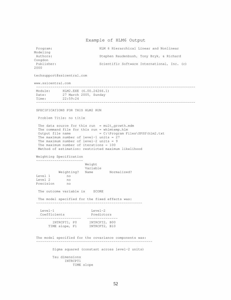
Example of HLM6 Growth Curve Output

52

Example of HLM6 Output

Program: HLM 6 Hierarchical Linear and NonlinearModelingAuthors: Stephen Raudenbush, Tony Bryk, & Richard

CongdonPublisher: Scientific Software International, Inc. (c)

2000

[email protected]

www.ssicentral.com------------------------------------------------------------------------------Module: HLM2.EXE (6.00.24266.1)Date: 27 March 2005, SundayTime: 22:59:24------------------------------------------------------------------------------

SPECIFICATIONS FOR THIS HLM2 RUN

Problem Title: no title

The data source for this run = mult_growth.mdmThe command file for this run = whlmtemp.hlmOutput file name = C:\Program Files\SPSS\hlm2.txtThe maximum number of level-1 units = 27The maximum number of level-2 units = 9The maximum number of iterations = 100Method of estimation: restricted maximum likelihood

Weighting Specification-----------------------

WeightVariable

Weighting? Name Normalized?Level 1 noLevel 2 noPrecision no

The outcome variable is SCORE

The model specified for the fixed effects was:----------------------------------------------------

Level-1 Level-2Coefficients Predictors

---------------------- ---------------INTRCPT1, P0 INTRCPT2, B00

TIME slope, P1 INTRCPT2, B10

The model specified for the covariance components was:---------------------------------------------------------

Sigma squared (constant across level-2 units)

Tau dimensionsINTRCPT1

TIME slope

53

Summary of the model specified (in equation format)---------------------------------------------------

Level-1 Model

Y = P0 + P1*(TIME) + E

Level-2 ModelP0 = B00 + R0P1 = B10 + R1

Level-1 OLS regressions-----------------------

Level-2 Unit INTRCPT1 TIME slope------------------------------------------------------------------------------

1 23.20513 1.153852 40.64103 1.230773 40.83333 2.500004 51.08974 1.192315 43.28205 1.461546 46.08974 2.192317 43.10256 3.076928 48.56410 2.923089 44.32051 2.11538

The average OLS level-1 coefficient for INTRCPT1 = 42.34758The average OLS level-1 coefficient for TIME = 1.98291

Least Squares Estimates-----------------------

sigma_squared = 89.34245


Least-squares estimates of fixed effects----------------------------------------------------------------------------

StandardFixed Effect Coefficient Error T-ratio d.f. P-value

----------------------------------------------------------------------------For INTRCPT1, P0

INTRCPT2, B00 42.347578 2.597158 16.305 25 0.000For TIME slope, P1

INTRCPT2, B10 1.982906 0.617904 3.209 25 0.004----------------------------------------------------------------------------


Least-squares estimates of fixed effects(with robust standard errors)----------------------------------------------------------------------------


----------------------------------------------------------------------------For INTRCPT1, P0


INTRCPT2, B10 1.982906 0.237255 8.358 25 0.000----------------------------------------------------------------------------

54

The robust standard errors are appropriate for datasets having a moderate tolarge number of level 2 units. These data do not meet this criterion.

The least-squares likelihood value = -96.005002Deviance = 192.01000Number of estimated parameters = 1

STARTING VALUES---------------

sigma(0)_squared = 19.26496

Tau(0)INTRCPT1,B0 50.16581 4.30883

TIME,B1 4.30883 -0.17102

New Tau(0)INTRCPT1,B0 12.65122 0.00000

TIME,B1 0.00000 0.11399


Estimation of fixed effects(Based on starting values of covariance components)----------------------------------------------------------------------------

Standard Approx.Fixed Effect Coefficient Error T-ratio d.f. P-value

----------------------------------------------------------------------------For INTRCPT1, P0


INTRCPT2, B10 1.982906 0.308211 6.434 8 0.000----------------------------------------------------------------------------

The value of the likelihood function at iteration 1 = -9.130511E+001The value of the likelihood function at iteration 2 = -8.567580E+001The value of the likelihood function at iteration 3 = -8.456389E+001The value of the likelihood function at iteration 4 = -8.430565E+001The value of the likelihood function at iteration 5 = -8.419899E+001

.

.

.

The value of the likelihood function at iteration 1935 = -8.393974E+001The value of the likelihood function at iteration 1936 = -8.393974E+001The value of the likelihood function at iteration 1937 = -8.393974E+001The value of the likelihood function at iteration 1938 = -8.393974E+001Iterations stopped due to small change in likelihood function

******* ITERATION 1939 *******

Sigma_squared = 14.89641

TauINTRCPT1,B0 55.31009 3.16901

TIME,B1 3.16901 0.18275

Tau (as correlations)

55

INTRCPT1,B0 1.000 0.997TIME,B1 0.997 1.000

----------------------------------------------------Random level-1 coefficient Reliability estimate

----------------------------------------------------INTRCPT1, B0 0.845

TIME, B1 0.242----------------------------------------------------

The value of the likelihood function at iteration 1939 = -8.393974E+001


Final estimation of fixed effects:----------------------------------------------------------------------------


----------------------------------------------------------------------------For INTRCPT1, P0


INTRCPT2, B10 1.982906 0.289768 6.843 8 0.000----------------------------------------------------------------------------


Final estimation of fixed effects(with robust standard errors)----------------------------------------------------------------------------


----------------------------------------------------------------------------For INTRCPT1, P0


INTRCPT2, B10 1.982906 0.237255 8.358 8 0.000----------------------------------------------------------------------------


Final estimation of variance components:-----------------------------------------------------------------------------Random Effect Standard Variance df Chi-square P-value

Deviation Component-----------------------------------------------------------------------------INTRCPT1, R0 7.43708 55.31009 8 49.99534 0.000

TIME slope, R1 0.42749 0.18275 8 7.95809 >.500level-1, E 3.85959 14.89641

-----------------------------------------------------------------------------

Statistics for current covariance components model--------------------------------------------------Deviance = 167.879480Number of estimated parameters = 4

56

Program: HLM 6 Hierarchical Linear and NonlinearModelingAuthors: Stephen Raudenbush, Tony Bryk, & Richard

CongdonPublisher: Scientific Software International, Inc. (c)

2000

[email protected]

www.ssicentral.com------------------------------------------------------------------------------Module: HLM2.EXE (6.00.24266.1)Date: 27 March 2005, SundayTime: 23: 3:57------------------------------------------------------------------------------

SPECIFICATIONS FOR THIS HLM2 RUN

Problem Title: no title

The data source for this run = mult_growth.mdmThe command file for this run = whlmtemp.hlmOutput file name = C:\Program Files\SPSS\hlm2.txtThe maximum number of level-1 units = 27The maximum number of level-2 units = 9The maximum number of iterations = 100Method of estimation: restricted maximum likelihood

Weighting Specification-----------------------

WeightVariable

Weighting? Name Normalized?Level 1 noLevel 2 noPrecision no


The model specified for the fixed effects was:----------------------------------------------------

Level-1 Level-2Coefficients Predictors

---------------------- ---------------INTRCPT1, P0 INTRCPT2, B00

GENDER, B01TIME slope, P1 INTRCPT2, B10

GENDER, B11

The model specified for the covariance components was:---------------------------------------------------------

Sigma squared (constant across level-2 units)

Tau dimensionsINTRCPT1

TIME slope

57

Summary of the model specified (in equation format)---------------------------------------------------

Level-1 Model

Y = P0 + P1*(TIME) + E

Level-2 ModelP0 = B00 + B01*(GENDER) + R0P1 = B10 + B11*(GENDER) + R1

Level-1 OLS regressions-----------------------Level-2 Unit INTRCPT1 TIME slope------------------------------------------------------------------------------

1 23.20513 1.153852 40.64103 1.230773 40.83333 2.500004 51.08974 1.192315 43.28205 1.461546 46.08974 2.192317 43.10256 3.076928 48.56410 2.923089 44.32051 2.11538

The average OLS level-1 coefficient for INTRCPT1 = 42.34758The average OLS level-1 coefficient for TIME = 1.98291

Least Squares Estimates-----------------------

sigma_squared = 71.19392


Least-squares estimates of fixed effects----------------------------------------------------------------------------


----------------------------------------------------------------------------For INTRCPT1, P0

INTRCPT2, B00 39.810256 3.110478 12.799 23 0.000GENDER, B01 5.708974 4.665717 1.224 23 0.234

For TIME slope, P1INTRCPT2, B10 1.507692 0.740031 2.037 23 0.053

GENDER, B11 1.069231 1.110046 0.963 23 0.346----------------------------------------------------------------------------


Least-squares estimates of fixed effects(with robust standard errors)----------------------------------------------------------------------------


----------------------------------------------------------------------------For INTRCPT1, P0



GENDER, B11 1.069231 0.311769 3.430 23 0.003----------------------------------------------------------------------------

58


The least-squares likelihood value = -89.040213Deviance = 178.08043Number of estimated parameters = 1

STARTING VALUES---------------

sigma(0)_squared = 19.26496

Tau(0)INTRCPT1,B0 48.85560 2.66898

TIME,B1 2.66898 -0.45254

New Tau(0)INTRCPT1,B0 12.38918 0.00000

TIME,B1 0.00000 0.05768


Estimation of fixed effects(Based on starting values of covariance components)----------------------------------------------------------------------------


----------------------------------------------------------------------------For INTRCPT1, P0



GENDER, B11 1.069231 0.599491 1.784 7 0.117----------------------------------------------------------------------------

The value of the likelihood function at iteration 1 = -8.355985E+001The value of the likelihood function at iteration 2 = -8.017255E+001The value of the likelihood function at iteration 3 = -7.916977E+001The value of the likelihood function at iteration 4 = -7.890406E+001The value of the likelihood function at iteration 5 = -7.882790E+001

.

.

.

The value of the likelihood function at iteration 2270 = -7.866254E+001The value of the likelihood function at iteration 2271 = -7.866254E+001The value of the likelihood function at iteration 2272 = -7.866254E+001The value of the likelihood function at iteration 2273 = -7.866254E+001Iterations stopped due to small change in likelihood function

59

******* ITERATION 2274 *******Sigma_squared = 13.81622

TauINTRCPT1,B0 55.27048 1.18597

TIME,B1 1.18597 0.02609

Tau (as correlations)INTRCPT1,B0 1.000 0.988

TIME,B1 0.988 1.000----------------------------------------------------Random level-1 coefficient Reliability estimate

----------------------------------------------------INTRCPT1, B0 0.855

TIME, B1 0.047----------------------------------------------------

The value of the likelihood function at iteration 2274 = -7.866254E+001

The outcome variable is SCOREFinal estimation of fixed effects:----------------------------------------------------------------------------


----------------------------------------------------------------------------For INTRCPT1, P0



GENDER, B11 1.069231 0.500866 2.135 7 0.070----------------------------------------------------------------------------

The outcome variable is SCOREFinal estimation of fixed effects(with robust standard errors)----------------------------------------------------------------------------


----------------------------------------------------------------------------For INTRCPT1, P0



GENDER, B11 1.069231 0.311769 3.430 7 0.013----------------------------------------------------------------------------


Final estimation of variance components:-----------------------------------------------------------------------------Random Effect Standard Variance df Chi-square P-value

Deviation Component-----------------------------------------------------------------------------INTRCPT1, R0 7.43441 55.27048 7 46.18915 0.000

TIME slope, R1 0.16152 0.02609 7 3.79932 >.500level-1, E 3.71702 13.81622

-----------------------------------------------------------------------------

Statistics for current covariance components model--------------------------------------------------Deviance = 157.325079Number of estimated parameters = 4

60

Workshop Contributors: This workshop was developed and delivered by a team from the College of Education:

Robert Dedrick, PhD, Associate Professor, Educational Measurement and Research, [email protected]

John Ferron, PhD, Associate Professor, Educational Measurement and Research, [email protected]

Melinda Hess, PhD, Director, Center for Research, Evaluation, Assessment and Measurement, [email protected]

Kristine Hogarty, PhD, Director of Assessment, Dean’s Office, [email protected]

Jeffrey Kromrey, PhD, Professor and Chair, Educational Measurement and Research, [email protected]

Tom Lang, Research Assistant, Educational Measurement and Research, [email protected]

John Niles, PhD, Visiting Professor, Educational Measurement and Research, [email protected]

Organizational Support for the workshop was provided by:

Lisa Adkins, Educational Measurement and Research, [email protected]

MULTILEVEL MODELING MULTILEVEL MODELING · PDF fileMULTILEVEL MODELING MULTILEVEL MODELING...

Documents

Transcript of MULTILEVEL MODELING MULTILEVEL MODELING · PDF fileMULTILEVEL MODELING MULTILEVEL MODELING...