Multilevel modeling in the presence of outliers: A ...Multilevel Modeling and Outliers 61 Multilevel...
36
Psicológica (2017), 38, 57-92. Multilevel modeling in the presence of outliers: A comparison of robust estimation methods Holmes Finch * Ball State University, USA Multilevel models (MLMs) have proven themselves to be very useful in social science research, as data from a variety of sources is sampled such that individuals at level-1 are nested within clusters such as schools, hospitals, counseling centers, and business entities at level-2. MLMs using restricted maximum likelihood estimation (REML) provide researchers with accurate estimates of parameters and standard errors at all levels of the data when the assumption of normality is met, and outliers are not present in the sample. However, if outliers at either levels 1 or 2 occur, the parameter estimates and standard errors produced by REML can both be compromised. Two estimation approaches for use when outliers are present have been proposed recently in the literature. Although the two methods, one based on ranks and the other on heavy tailed distributions of model errors, show promise, neither has heretofore been studied comprehensively across a wide variety of data conditions, nor have they been compared with one another. Thus, the purpose of the current study was to compare the rank and heavy tailed based estimation techniques with one another, and with REML, in terms of their ability to estimate level-1 fixed effects, under a variety of data conditions. Results of the study revealed that the rank based and heavy tailed method provide less biased estimates than REML when outliers are present, and that the rank approaches yield smaller standard errors than the heavy tailed approach in the presence of outliers. Implications of these results are discussed. Frequently in psychological and social science research, data are collected whereby individuals are sampled within clusters, such as schools, hospitals, therapists, states, or nations. Standard statistical models (e.g. linear regression, logistic regression, and analysis of variance) do not properly account for the nested structure of such data, and can yield biased * Corresponding author: Holmes Finch PHD. Department of Educational Psychology. Ball State University, USA. E-mail: [email protected]
Transcript of Multilevel modeling in the presence of outliers: A ...Multilevel Modeling and Outliers 61 Multilevel...
Psicológica (2017), 38, 57-92.
Multilevel modeling in the presence of outliers: A comparison of robust estimation methods
Holmes Finch*
Ball State University, USA
Multilevel models (MLMs) have proven themselves to be very useful in social science research, as data from a variety of sources is sampled such that individuals at level-1 are nested within clusters such as schools, hospitals, counseling centers, and business entities at level-2. MLMs using restricted maximum likelihood estimation (REML) provide researchers with accurate estimates of parameters and standard errors at all levels of the data when the assumption of normality is met, and outliers are not present in the sample. However, if outliers at either levels 1 or 2 occur, the parameter estimates and standard errors produced by REML can both be compromised. Two estimation approaches for use when outliers are present have been proposed recently in the literature. Although the two methods, one based on ranks and the other on heavy tailed distributions of model errors, show promise, neither has heretofore been studied comprehensively across a wide variety of data conditions, nor have they been compared with one another. Thus, the purpose of the current study was to compare the rank and heavy tailed based estimation techniques with one another, and with REML, in terms of their ability to estimate level-1 fixed effects, under a variety of data conditions. Results of the study revealed that the rank based and heavy tailed method provide less biased estimates than REML when outliers are present, and that the rank approaches yield smaller standard errors than the heavy tailed approach in the presence of outliers. Implications of these results are discussed.
Frequently in psychological and social science research, data are collected whereby individuals are sampled within clusters, such as schools, hospitals, therapists, states, or nations. Standard statistical models (e.g. linear regression, logistic regression, and analysis of variance) do not properly account for the nested structure of such data, and can yield biased
* Corresponding author: Holmes Finch PHD. Department of Educational Psychology. Ball State University, USA. E-mail: [email protected]
H. Finch 58
parameter estimates, and incorrect standard errors (Bryk & Raudenbush, 2001). In order to address such problems, researchers must make use of multilevel models, which are designed to deal with this data structure by accounting for sources of variance in the dependent variable from the different levels (e.g. students and schools). Such models have been shown to yield accurate parameter estimates and standard errors at each level of the data structure (Snijders & Bosker, 2012). Given their great utility in many research contexts, these multilevel models have become increasingly popular in social science research, and are available in a variety of widely used software packages, such as R, HLM, SAS, SPSS, and Mplus.
Although they have been shown to be quite useful, multilevel models are susceptible to outliers occurring at each level of the data, leading to parameter estimation bias and inflated standard errors (e.g. Kloke, McKean, & Rashid, 2009; Seltzer & Choi, 2003). In turn, outliers occur frequently in social science research (Finch, 2012; Osborne & Overbay, 2008), and thus cannot be ignored. The purpose of this simulation study was to examine the performance of two methods for dealing with outliers in the context of multilevel data, including an approach based on ranks, and another based on heavy tailed data distributions. These alternatives to the standard maximum likelihood estimation of model parameters were selected for the current study because one of them (the heavy tailed method) has been suggested for use in a variety of contexts, including multilevel and latent variable models, whereas the other (rank based) is relatively new in the context of multilevel modeling. In addition, these methods have not been compared with one another, nor has either been thoroughly studied with multilevel data under a variety of conditions. It should be noted, however, that the heavy tailed approach has been the subject of several studies focused on latent variable and standard linear models. Following is a brief description of multilevel models, and methods for estimating the parameters, including those based on ranks and heavy tails. Next is a review of prior research on the performance of these methods, followed by a description of the goals of the current study, and the method used to address these goals. The simulation results are then presented and discussed, including their implications for practice, as well as directions for future research.
Multilevel models Multilevel models (MLMs), sometimes also referred to as mixed
effects models, are used in the analysis of data in which individuals (level-1) are nested within clusters (level-2), and the clusters could themselves be nested within higher order clusters (level-3). MLMs can also be used in the
Multilevel Modeling and Outliers 59
case of longitudinal data, where measurements taken at different points in time are nested within the individuals on whom they were made. In these situations, modeling of the dependent variable must account for the nested data structure in order to ensure that standard errors and model parameters are accurately estimated (Snijders & Bosker, 2012). One of the most common such MLMs is the random intercept model linking an independent variable, x, with a dependent variable y, which takes the form:
𝑦!" = 𝛽!! + 𝛽!𝑥!" + 𝜀!" (1) where
𝑦!" =Dependent variable value for individual i in cluster j 𝛽!! =Intercept for cluster j 𝛽! =Slope relating independent variable x to dependent variable y 𝑥!" =Value of x for individual i in cluster j 𝜀!" =Random error for individual i in cluster j In model (1), 𝛽!! can be expressed as
𝛽!! = 𝛾!! + 𝑈!! (2) where
𝛾!! =Mean intercept across clusters 𝑈!! =Unique effect of cluster j on the intercept
The parameter 𝛾!! is a fixed effect, meaning that it takes the same
value for all clusters, and it is estimated in a separate step. On the other hand, 𝑈!! is a random effect that varies across clusters. In the context of students nested within schools, this would mean that model intercepts would differ across schools, with part of the intercept including a common component across schools (𝛾!!), as well as a component unique to the individual school (𝑈!!). In model (1), 𝛽! is a fixed effect meaning that it is constant across clusters. Again, in the school research context, this would mean that the relationship between the independent and dependent variables is the same for all schools. It is also possible to fit a random coefficients model in which 𝛽! has both fixed and random components, just as we have here for 𝛽!!. This random coefficients model would thus allow for differing relationships between the independent and dependent variables across schools. The error term, 𝜀!", is a random effect and assumed to be normally and independently distributed across individuals with 𝜀!"~𝑁(𝟎,Λ!).
H. Finch 60
Likewise, 𝑈!!~𝑁(𝟎,Ψ), and is assumed to be independent across clusters. It should be noted that the assumption of normally distributed errors applies only to the maximum likelihood (ML) estimator, and not to the rank based approach that is described below.
The model parameters in (1) and (2) are typically estimated by maximum likelihood (ML) or restricted ML (REML) estimation. With regard to estimating the model parameters themselves ( 𝛽!, 𝛾!!), ML and REML provide essentially identical results. However, they differ in terms of how the standard errors of these parameters are calculated. Specifically, the degrees of freedom used in ML do not account for the fact that the parameters themselves are being estimated, leading to a negative bias in the standard error estimates (Kreft & de Leeuw, 1998). In contrast, REML standard error estimates do use degrees of freedom that account for the estimation of the model parameters, thereby producing unbiased estimates (Snijders & Bosker, 2012; Lindstrom & Bates, 1988). REML was used in the current study.
Outliers and multilevel model parameter estimation When outliers are present in the data, REML and ML estimates can be
adversely impacted (Pinheiro, Liu, and Wu, 2001). In the context of MLM, outliers can occur at each level of the data. So, for example, it is possible to have outliers among the individuals, and among the clusters within which the individuals are nested. Prior work has shown that the presence of outliers has a detrimental impact particularly on the estimation of standard errors of parameters in the 2-level MLM (e.g. Kloke, et al., 2009; Pinheiro, et al., 2001). A more thorough review of this prior research on the impact of outliers on each of several MLM estimation methods is presented below. At this point, it is important to note that outliers do lead to estimation problems for ML/REML based MLM estimation algorithms, and as such researchers have developed alternative estimators for when such outliers are present in the data. These approaches can be considered in two broad categories of estimators, one based on nonparametric R estimators, and the other on multivariate heavy tailed distributions, such as the t, the Cauchy, or the slash distribution. Following is a description of each of these two families of MLM estimators, followed by a description of the simulation study designed to compare their performance in estimating fixed effects parameters and their associated standard errors. Results of the simulation study are then presented, and discussed in light of previous literature, with recommendations for practice.
Multilevel Modeling and Outliers 61
Multilevel modeling using heavy tailed distributions There is a great deal of literature with respect to the fitting of models
using data containing outlying observations. Much of this work has focused on single level models, such as linear regression (see Fox, 2016 for a thorough discussion of dealing with outliers in the single level linear regression context). One approach for handling outliers with multilevel models suggested by Lange, Little, and Taylor (1989) involves adjusting the distributions of error terms (e.g., 𝜀!" and 𝑈!!) from multivariate normal to a heavy tailed distribution such as the multivariate t with 𝜐 degrees of freedom. Very simply, modeling the error terms using a heavy tailed distribution such as the multivariate t, rather than the multivariate normal which has lighter tails, better accommodates more extreme values (i.e. outliers). The result of using such a distribution for errors should be more accurate parameter and standard error estimates (Lange, et al., 1989). Pinheiro, et al (2001) extended the work of Lange, et al (1989) by describing a ML algorithm for estimating the parameters in the model expressed in equations (1) and (2), using the multivariate t distribution. A number of authors have considered the performance of models based on heavy tailed distributions, particularly in the context of latent variable and growth curve modeling, and found that when outliers are present, such approaches yielded more accurate parameter estimates and smaller standard errors than did standard ML based methods assuming normally distributed errors (Tong & Zhang, 2012; Song, Zhang, & Qu, 2007; Yuan, Bentler, & Chan, 2004; Yuan & Bentler, 1998).
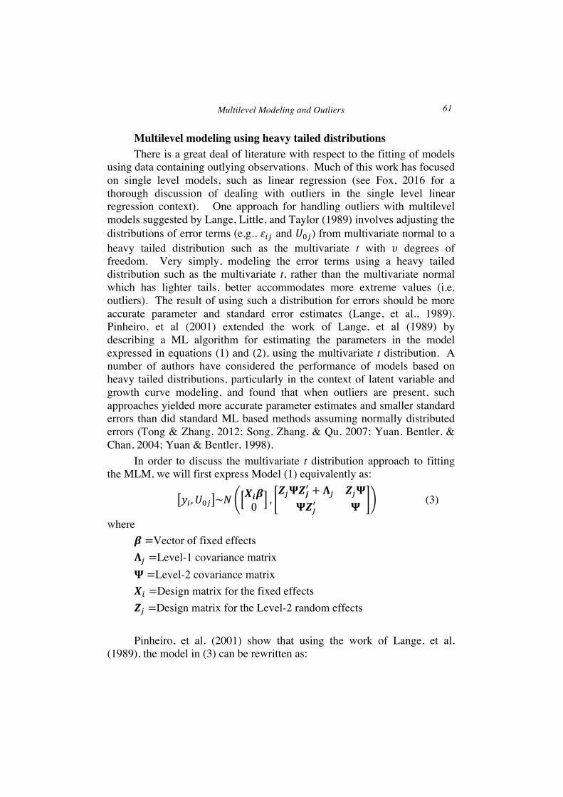
In order to discuss the multivariate t distribution approach to fitting the MLM, we will first express Model (1) equivalently as:
𝑦! ,𝑈!! ~𝑁𝑿𝒊𝜷0 ,
𝒁!𝚿𝒁𝒋! + 𝚲! 𝒁!𝚿𝚿𝒁!! 𝚿 (3)
where 𝜷 =Vector of fixed effects 𝚲! =Level-1 covariance matrix 𝚿 =Level-2 covariance matrix 𝑿! =Design matrix for the fixed effects 𝒁! =Design matrix for the Level-2 random effects Pinheiro, et al. (2001) show that using the work of Lange, et al.
(1989), the model in (3) can be rewritten as:
H. Finch 62
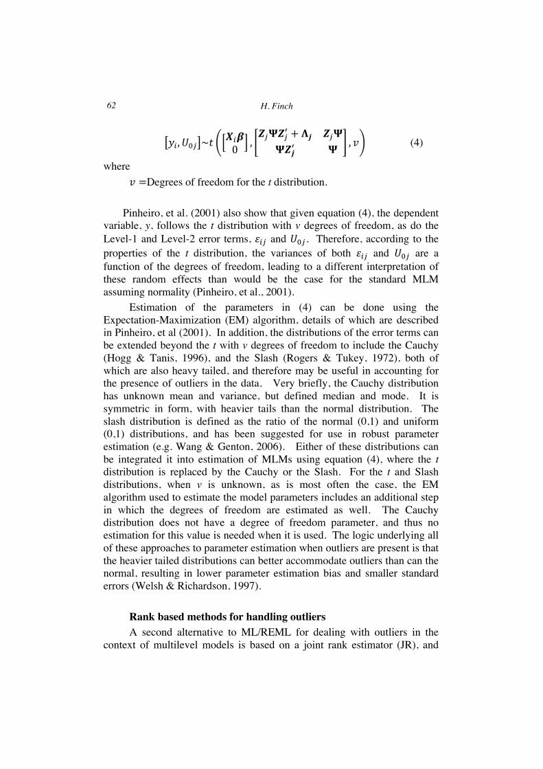
𝑦! ,𝑈!! ~𝑡𝑿!𝜷0 ,
𝒁!𝚿𝒁!! + 𝚲𝒋 𝒁!𝚿𝚿𝒁𝒋! 𝚿 , 𝑣 (4)
where 𝑣 =Degrees of freedom for the t distribution.
Pinheiro, et al. (2001) also show that given equation (4), the dependent
variable, y, follows the t distribution with v degrees of freedom, as do the Level-1 and Level-2 error terms, 𝜀!" and 𝑈!!. Therefore, according to the properties of the t distribution, the variances of both 𝜀!" and 𝑈!! are a function of the degrees of freedom, leading to a different interpretation of these random effects than would be the case for the standard MLM assuming normality (Pinheiro, et al., 2001).
Estimation of the parameters in (4) can be done using the Expectation-Maximization (EM) algorithm, details of which are described in Pinheiro, et al (2001). In addition, the distributions of the error terms can be extended beyond the t with v degrees of freedom to include the Cauchy (Hogg & Tanis, 1996), and the Slash (Rogers & Tukey, 1972), both of which are also heavy tailed, and therefore may be useful in accounting for the presence of outliers in the data. Very briefly, the Cauchy distribution has unknown mean and variance, but defined median and mode. It is symmetric in form, with heavier tails than the normal distribution. The slash distribution is defined as the ratio of the normal (0,1) and uniform (0,1) distributions, and has been suggested for use in robust parameter estimation (e.g. Wang & Genton, 2006). Either of these distributions can be integrated it into estimation of MLMs using equation (4), where the t distribution is replaced by the Cauchy or the Slash. For the t and Slash distributions, when v is unknown, as is most often the case, the EM algorithm used to estimate the model parameters includes an additional step in which the degrees of freedom are estimated as well. The Cauchy distribution does not have a degree of freedom parameter, and thus no estimation for this value is needed when it is used. The logic underlying all of these approaches to parameter estimation when outliers are present is that the heavier tailed distributions can better accommodate outliers than can the normal, resulting in lower parameter estimation bias and smaller standard errors (Welsh & Richardson, 1997).
Rank based methods for handling outliers A second alternative to ML/REML for dealing with outliers in the
context of multilevel models is based on a joint rank estimator (JR), and
Multilevel Modeling and Outliers 63
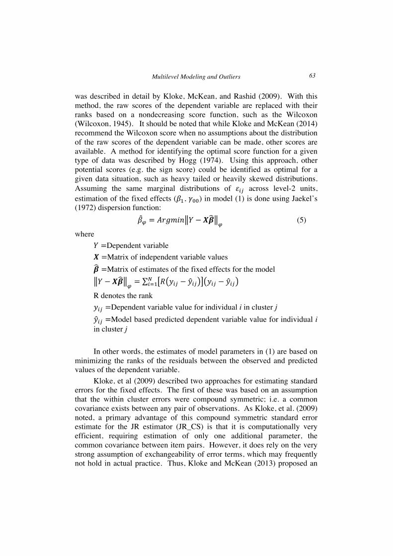
was described in detail by Kloke, McKean, and Rashid (2009). With this method, the raw scores of the dependent variable are replaced with their ranks based on a nondecreasing score function, such as the Wilcoxon (Wilcoxon, 1945). It should be noted that while Kloke and McKean (2014) recommend the Wilcoxon score when no assumptions about the distribution of the raw scores of the dependent variable can be made, other scores are available. A method for identifying the optimal score function for a given type of data was described by Hogg (1974). Using this approach, other potential scores (e.g. the sign score) could be identified as optimal for a given data situation, such as heavy tailed or heavily skewed distributions. Assuming the same marginal distributions of 𝜀!" across level-2 units, estimation of the fixed effects (𝛽!, 𝛾!!) in model (1) is done using Jaekel’s (1972) dispersion function:
𝛽! = 𝐴𝑟𝑔𝑚𝑖𝑛 𝑌 − 𝑿𝜷!
(5)
where 𝑌 =Dependent variable 𝑿 =Matrix of independent variable values 𝜷 =Matrix of estimates of the fixed effects for the model 𝑌 − 𝑿𝜷
!= 𝑅 𝑦!" − 𝑦!" 𝑦!" − 𝑦!"!
!!!
R denotes the rank 𝑦!" =Dependent variable value for individual i in cluster j 𝑦!" =Model based predicted dependent variable value for individual i in cluster j
In other words, the estimates of model parameters in (1) are based on
minimizing the ranks of the residuals between the observed and predicted values of the dependent variable.
Kloke, et al (2009) described two approaches for estimating standard errors for the fixed effects. The first of these was based on an assumption that the within cluster errors were compound symmetric; i.e. a common covariance exists between any pair of observations. As Kloke, et al. (2009) noted, a primary advantage of this compound symmetric standard error estimate for the JR estimator (JR_CS) is that it is computationally very efficient, requiring estimation of only one additional parameter, the common covariance between item pairs. However, it does rely on the very strong assumption of exchangeability of error terms, which may frequently not hold in actual practice. Thus, Kloke and McKean (2013) proposed an
H. Finch 64
alternative method for calculating standard errors based on the well-known sandwich estimator approach (JR_SE). The primary advantage of JR_SE is that it does not require any additional assumptions about the data beyond those of ML/REML, unlike JR_CS. Kloke and McKean (2013) conducted a simulation study comparing the performance of JR_CS and JR_SE, and found that JR_SE worked well for larger sample sizes (e.g. greater than or equal to 50 level-2 units). However, for situations with fewer level-2 units, JR_SE yielded somewhat larger standard error estimates than JR_CS, thereby leading to more conservative inference with regard to the statistical significance of the parameter estimates. On the other hand, Kloke and McKean (2013) also found that when the exchangeability assumption was violated, JR_CS standard error estimates were inflated. The final recommendation from the Kloke and McKean paper was that JR_SE should be used as the default, but that when the level-2 sample size is small, researchers should consider using the JR_CS estimator, unless they know that the exchangeability assumption has been violated. Given this pattern of mixed results, both approaches for estimating standard errors were used in the current study.
Prior research on alternatives for MLM estimation with outliers There has been relatively little in the way of empirical simulation
research examining the performance of either the heavy tailed or the rank based methods with MLMs, with no work comparing these approaches to one another. As noted above, research has examined performance of the heavy tailed method with outliers in the context of latent variable and single level models, and found that they work well under many conditions in these contexts. With respect to MLMs, Pinheiro, et al. (2001) conducted a simulation study comparing the heavy tailed approach using the t distribution with v estimated by the EM algorithm with REML. The researchers manipulated a variety of factors including magnitude of the outlier at both levels 1 and 2, and the proportion of data at each level that were outliers. The results of the study demonstrated that for data with outliers, the heavy tailed t approach provided more accurate model parameter estimates than did the normal based method, particularly for a greater magnitude of contamination. As with the heavy tailed methods, some simulation work has been conducted comparing the performance of the rank based MLM estimators with REML (Kloke, et al., 2009). In this study, outliers were simulated at level-1 only, with one set of conditions for magnitude of the outlier effect, and percent of observations simulated to be outliers. The results of this study demonstrated that when no outliers were
Multilevel Modeling and Outliers 65
present, REML produced somewhat more efficient estimates than did the rank approach. However, in the presence of outliers this pattern was reversed, with the rank based estimates being much more efficient than those yielded by REML. Coverage rates for both methods over all simulation conditions were essentially at the nominal 95% level. As discussed above briefly, in a second simulation study designed to compare the compound symmetry (JR_CS) and sandwich estimator (JR_SE) methods for estimating standard errors of the rank based estimators, Kloke and McKean (2013) found that the two estimators produced similar results under many conditions. However, for larger Level-2 sample sizes, JR_SE yielded somewhat more accurate Type I error and power results than did JR_CS. For this reason, they concluded that researchers are essentially always safe using JR_SE, but may not always be so with JR_CS, depending upon the sample size (Kloke & McKean, 2013). Interested readers are encouraged to review Pinheiro, et al. (2001), Kloke, et al., (2009), and Kloke and McKean, (2013) for details of the simulation study designs used.
Study goals The purpose of this study was to investigate and compare the
performance of heavy tailed and rank based methods for handling outliers at both levels 1 and 2 in a multilevel data context. The heavy tailed estimation procedure was selected for inclusion in this study because it has been shown to be effective for dealing with outliers, particularly in the context of latent variable models. It should be noted that some of this earlier research has shown that when no outliers are present in the data, the standard errors of heavy tailed estimates tended to be larger than those of the REML based estimates (Pinheiro, 2001). The rank based methods for parameter estimation in the context of MLMs are much newer, and have not been investigated over a wide range of conditions. In addition, prior research in this area has involved relatively small simulation studies comparing only one of the alternatives to the standard REML estimation approach (e.g. Tong & Zhang, 2012; Kloke, et al., 2009; Pinheiro, et al, 2001; Staudenmayer, Lake & Wand, 2009), but not comparing them all with one another, nor examining them under a variety of conditions with respect to sample size, and type and magnitude of outliers. Given the combination of their promise with the need for direct comparisons of the methods under a wider array of conditions, the current study adds four new pieces to the existing literature: (1) It simultaneously compared the impact of outliers on fixed effects estimation for the rank based, heavy tailed, and REML estimation methods, which has not been done heretofore, (2) It included a
H. Finch 66
wider array of simulation conditions than was the case in previous research, (3) It examined the impact of level-2 outliers on level-1 fixed effect parameter estimation, which was not done with the heavy tailed methods in prior research, and which was done with the rank based methods for just a small number of conditions, and (4) It included two additional heavy tailed estimation approaches that haven’t been studied before (Cauchy and Slash), and examined standard error estimates for all of the methods, which hadn’t been done previously for the heavy tailed estimators.
Results of prior research provide some information that can be used in constructing hypotheses about outcomes in the present study. First of all, given results in Pinheiro, et al. (2001) and Kloke, et al. (2009), it was anticipated that in the presence of outliers, the rank and heavy tailed estimation techniques would provide less biased estimates of fixed effects than would the standard REML based approach. Furthermore, it was hypothesized that a greater magnitude of outliers would affect all of the methods deleteriously, but REML the most. In addition, it was expected that for smaller sample sizes JR_SE would produce somewhat larger standard error estimates than JR_CS, but that with larger samples this difference would be diminished. Finally, it was not clear what results to expect in regards to the comparative performance of the rank and heavy tailed estimators, given that they have not been compared with one another previously, and both have performed better than REML with outliers.
METHODS A Monte Carlo simulation with 1000 replications per combination of
conditions was used to address the study goals outlined above. A total of 288 different combinations of simulation conditions (described below) were used, leading to 288,000 replications for each of the estimation methods included in the study. Data were generated and analyzed using the R software package, version 3.02 (R Core Development Team, 2015) for a two level model with equal numbers of level-1 units within each level-2 unit. The data generating model was based on equations (6) and (7):
𝑦!" = 𝛽!! + 𝛽!𝑥!!" + 𝛽!𝑥!!" + 𝜀!" (6) 𝛽!! = 𝛾!! + 𝑈!! (7)
where 𝛾!! =1
𝜀!"~𝑁 0,𝜎!!"!
Multilevel Modeling and Outliers 67
𝑈!!~𝑁 0,𝜎!!!!
𝑥!!"~𝑁 0,1 𝑥!!"~𝑁 0,1 𝛽! =1 𝛽! = 0.5 The variables 𝑥! and 𝑥! were simulated to have a correlation of 0.5. Focus on this study was on the estimation of the fixed effects 𝛾!!, 𝛽!,
and 𝛽!. This focus was of primary interest for two reasons. First, in practice, researchers are most frequently interested in the fixed effects when interpreting results from multilevel modeling, as they want to know which of the independent variables are associated with the dependent variable. Second, as noted by Pinheiro, et al. (2001) the random effects obtained from the heavy tailed methods are not directly comparable to those obtained using REML, and thus do not lend themselves to comparison in the simulation context. This does not mean that random effect estimation is not an important issue, but rather only that the current study focused on fixed effects estimation for ease of interpretation, and comparison of the methods with one another. In addition, the data generating model did not include random effects for 𝛽! or 𝛽!. The decision was made to simulate them only as fixed effects simply to keep the scope of the study manageable. It is definitely of interest to examine estimation of these parameters when their values can vary across clusters, and future research should do so. However, given the fairly large number of conditions that were manipulated in the study, and the fact that the heavy tailed and rank based methods have not been previously compared with one another, it was felt that generating 𝛽! and 𝛽! as fixed effects was best in this case. Other study conditions were manipulated as described below.
Level-1 and Level-2 sample size Level-1 sample sizes (N1) were 5, 15, 25, or 50 within each level-2
unit. Level-2 sample sizes (N2) were 5, 15, 25, and 50 units as well, leading to total samples sizes ranging from 25 to 2500. These values were selected to represent a range from very small to fairly large samples, and are representative of values that have been seen in practice, and in prior simulation studies (e.g. Hastings, Helm, Mills, Serbin, Stack, & Schwartzman, 2015; Qian, Ticha, Larson, Stancliffe, & Wuorio, 2015; Simons, Wills, & Neal, 2014; Kloke, et al, 2009; Pinheiro, et al., 2001). In
H. Finch 68
addition, Maas and Hox (2005) reported that with N2 as small as 20, estimates for the fixed effects will be accurate for REML estimates. Thus, values for N2 above and below 20 were selected in order to assess the performance of the heavy tailed and rank based methods, which have not been as thoroughly investigated as has ML/REML.
Intraclass correlation The unconditional intraclass correlation (ICC) reflects the strength of
relationship of dependent variable values for individuals within the same level-2 unit, and was manipulated to be 0.1 and 0.25. These values have been used in prior simulation studies (e.g. French & Finch, 2012), and represent a range of values seen in practice with respect to clusters of individuals (e.g. Kivlighan, Coco, & Gullo, 2015; Thompson, Fernald, & Mold, 2012; Hedges & Hedberg, 2007). The ICC values are obtained through manipulation of 𝜎!!"
! and 𝜎!!!! .
Percentage and Magnitude of outlying observations Outliers were simulated at level-1 and level-2 by manipulating the
variance of the error terms, 𝜀!" and 𝑈!!, respectively. To simulate level-1outliers, 0%, 10%, and 20% of observations was generated such that 𝜀!"~𝑁 0,𝜎! , where 𝜎! took the values 5, 10, 25, and 50 times larger than 𝜎! for the other level-1 units. Similarly, for level-2 outliers, 0%, 10%, and 20% of the data was generated with 𝑈!"~𝑁 0,𝜎! , where 𝜎! also took the values 5, 10, 25, and 50 larger than 𝜎! for the other level-2 units. These variance values were taken from prior resarch using similar methods and magnitudes for generating outliers in multilevel models (e.g. Kloke, et al.2009; Pinheiro, et al., 2001). In addition, there was a set of simulations for which no outliers were present. When outliers were simulated to be present, the level-1 and level-2 conditions were not crossed with one another. This decision to examine the two types of outliers separately was made because the focus of this study was on studying the impact of Level-1 and Level-2 outliers, respectively, and as Pinheiro, et al. (2001) noted, the two types of outliers can be difficult to disentangle from one another when they appear together. In addition, a small number of simulations were conducted in which both level-1 and level-2 outliers were simulated to be present simultaneously. The results were generally similar to those for the level-1 outliers, which are presented below. Therefore, it was felt that including results for the Level-1 and Level-2 outliers together would be
Multilevel Modeling and Outliers 69
somewhat redundant with the level-1 outlier results, and would unnecessarily lengthen the manuscript.
Model parameter estimation methods The parameter estimation methods used in this study included REML
with the R lmer package. The maximum number of iterations for REML estimation was set at 100, with a tolerance value of 1e-6. Across all simulation conditions in the current study, REML converged for all replications. Rank based estimation using both JR_CS and JR_SE standard error estimation was conducted with the R jrfit package (Kloke & McKean, 2013). Estimation using heavy tailed distributions was done using the heavy package in R. For the heavy tailed approaches, Student’s t with degrees of freedom estimated by the EM algorithm, the Cauchy distribution, and the Slash distribution with degrees of freedom estimated by the EM algorithm were all used. The maximum number of iterations for each distribution was set at the default of 4000, with tolerance of 1e-6. As was true of both REML and the rank based methods, the convergence rate was 100% across all replications under all simulation conditions. Finally, outliers were also identified using studentized residuals (e.g. Fox, 2016) for the level-1 observations. For each simulated data point, the studentized residuals based on the REML estimated model were calculated, and individuals with absolute values greater than or equal to 2 were removed, after which the model was estimated again using REML. This aspect of the simulation study was included to represent the practice whereby a researcher would attempt to identify and then remove any outlying observations. The R package HLMdiag was used in conjunction with lmer to identify the outliers, and lmer was used to estimate the model after the outliers were removed.
Study outcomes One primary study outcome was absolute estimation bias for the fixed
effects 𝛾!!, 𝛽!, and 𝛽!, which was calculated for each parameter at each replication as:
|𝜃 − 𝜃| (8) where
𝜃 =Data generating value at each replication 𝜃 =Model estimated value at each replication
H. Finch 70
A second study outcome of interest was the empirical standard error, which was calculated as the standard deviation of the parameter estimates across the 1000 replications for each combination of conditions. The final outcome to be examined in this study were the 95% coverage rates for 𝛾!!, 𝛽!, and 𝛽!. For each simulation replication, the 95% confidence interval was calculated for each of the model parameter estimates, after which it was determined whether the data generating value was within the interval. The coverage rates were then calculated as the proportion of replications for which the data generating value was within the 95% confidence interval. In order to ascertain which of the manipulated factors and their interactions contributed most to parameter estimation bias, analysis of variance (ANOVA) was used, in conjunction with the 𝜂! effect size. The ANOVA models treated estimation bias of the model parameters as the dependent variable, and the manipulated study factors and their interactions as the independent variables. The purpose behind using the ANOVA in this case was to identify the main effects and interactions of the factors manipulated in the simulation study that were associated with parameter estimation bias. In this way, the factors and interactions that were not identified as statistically significant using the ANOVA could be ignored, so that focus would only be on those that actually influenced estimation bias. Results in the tables are described only for those main effects and interactions that were identified as statistically significantly related to absolute bias, and were averaged across those main effects and interactions that were not identified by ANOVA as being related to bias. The effect size value was also included in the reporting of results in order to provide some information regarding the relative magnitude of the effect of the significant manipulated factors and interactions on estimation bias. Use of inferential techniques such as ANOVA in Monte Carlo simulation research has been suggested for this purpose of highlighting only those main effects and interactions that are related to the outcome variables of interest (e.g., Paxton, Curran, Bollen, Kirby, & Chen, 2001).
RESULTS No outliers ANOVA results showed that when there were no outliers present (0%
contamination) in the population, the interaction of ICC by method of estimation was significantly related to the estimation bias for 𝛾!! (𝐹!,!" = 5.883,𝑝 = 0.037, 𝜂! = 0.455). With regard to estimation bias for 𝛽!, only the main effect of method was statistically significant (𝐹!,!" =
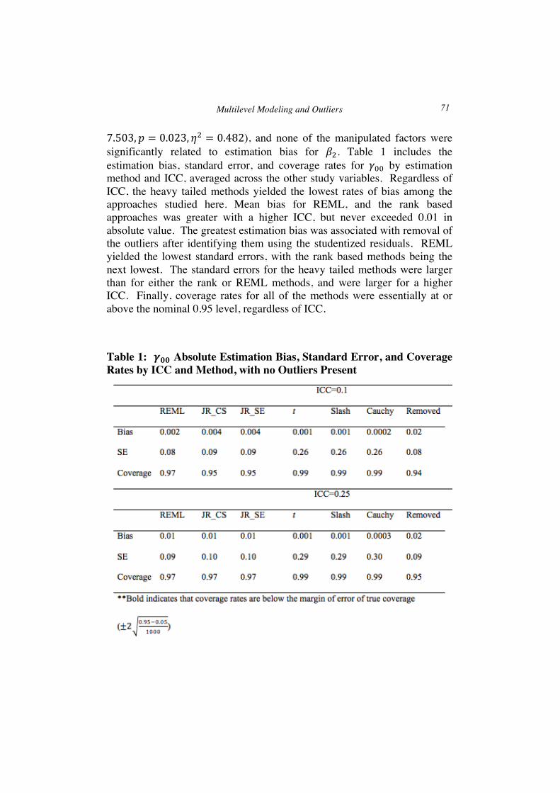
Multilevel Modeling and Outliers 71
7.503,𝑝 = 0.023, 𝜂! = 0.482), and none of the manipulated factors were significantly related to estimation bias for 𝛽!. Table 1 includes the estimation bias, standard error, and coverage rates for 𝛾!! by estimation method and ICC, averaged across the other study variables. Regardless of ICC, the heavy tailed methods yielded the lowest rates of bias among the approaches studied here. Mean bias for REML, and the rank based approaches was greater with a higher ICC, but never exceeded 0.01 in absolute value. The greatest estimation bias was associated with removal of the outliers after identifying them using the studentized residuals. REML yielded the lowest standard errors, with the rank based methods being the next lowest. The standard errors for the heavy tailed methods were larger than for either the rank or REML methods, and were larger for a higher ICC. Finally, coverage rates for all of the methods were essentially at or above the nominal 0.95 level, regardless of ICC.
Table 1: 𝜸𝟎𝟎 Absolute Estimation Bias, Standard Error, and Coverage Rates by ICC and Method, with no Outliers Present
H. Finch 72
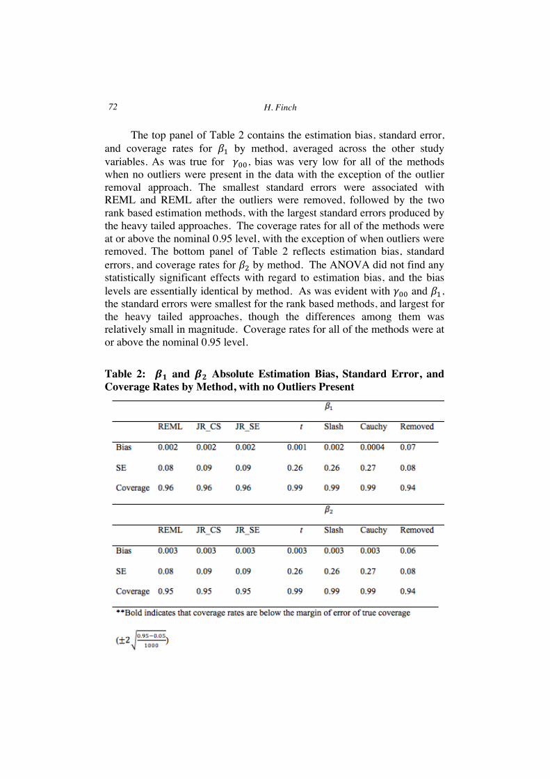
The top panel of Table 2 contains the estimation bias, standard error, and coverage rates for 𝛽! by method, averaged across the other study variables. As was true for 𝛾!!, bias was very low for all of the methods when no outliers were present in the data with the exception of the outlier removal approach. The smallest standard errors were associated with REML and REML after the outliers were removed, followed by the two rank based estimation methods, with the largest standard errors produced by the heavy tailed approaches. The coverage rates for all of the methods were at or above the nominal 0.95 level, with the exception of when outliers were removed. The bottom panel of Table 2 reflects estimation bias, standard errors, and coverage rates for 𝛽! by method. The ANOVA did not find any statistically significant effects with regard to estimation bias, and the bias levels are essentially identical by method. As was evident with 𝛾!! and 𝛽!, the standard errors were smallest for the rank based methods, and largest for the heavy tailed approaches, though the differences among them was relatively small in magnitude. Coverage rates for all of the methods were at or above the nominal 0.95 level.
Table 2: 𝜷𝟏 and 𝜷𝟐 Absolute Estimation Bias, Standard Error, and Coverage Rates by Method, with no Outliers Present
Multilevel Modeling and Outliers 73
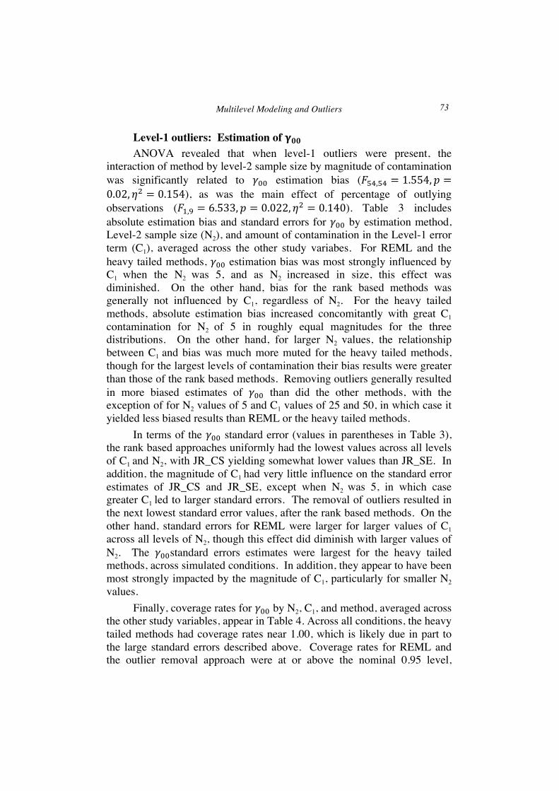
Level-1 outliers: Estimation of 𝛄𝟎𝟎 ANOVA revealed that when level-1 outliers were present, the
interaction of method by level-2 sample size by magnitude of contamination was significantly related to 𝛾!! estimation bias (𝐹!",!" = 1.554,𝑝 =0.02, 𝜂! = 0.154), as was the main effect of percentage of outlying observations (𝐹!,! = 6.533,𝑝 = 0.022, 𝜂! = 0.140). Table 3 includes absolute estimation bias and standard errors for 𝛾!! by estimation method, Level-2 sample size (N2), and amount of contamination in the Level-1 error term (C1), averaged across the other study variabes. For REML and the heavy tailed methods, 𝛾!! estimation bias was most strongly influenced by C1 when the N2 was 5, and as N2 increased in size, this effect was diminished. On the other hand, bias for the rank based methods was generally not influenced by C1, regardless of N2. For the heavy tailed methods, absolute estimation bias increased concomitantly with great C1 contamination for N2 of 5 in roughly equal magnitudes for the three distributions. On the other hand, for larger N2 values, the relationship between C1 and bias was much more muted for the heavy tailed methods, though for the largest levels of contamination their bias results were greater than those of the rank based methods. Removing outliers generally resulted in more biased estimates of 𝛾!! than did the other methods, with the exception of for N2 values of 5 and C1 values of 25 and 50, in which case it yielded less biased results than REML or the heavy tailed methods.
In terms of the 𝛾!! standard error (values in parentheses in Table 3), the rank based approaches uniformly had the lowest values across all levels of C1 and N2, with JR_CS yielding somewhat lower values than JR_SE. In addition, the magnitude of C1 had very little influence on the standard error estimates of JR_CS and JR_SE, except when N2 was 5, in which case greater C1 led to larger standard errors. The removal of outliers resulted in the next lowest standard error values, after the rank based methods. On the other hand, standard errors for REML were larger for larger values of C1 across all levels of N2, though this effect did diminish with larger values of N2. The 𝛾!!standard errors estimates were largest for the heavy tailed methods, across simulated conditions. In addition, they appear to have been most strongly impacted by the magnitude of C1, particularly for smaller N2 values.
Finally, coverage rates for 𝛾!! by N2, C1, and method, averaged across the other study variables, appear in Table 4. Across all conditions, the heavy tailed methods had coverage rates near 1.00, which is likely due in part to the large standard errors described above. Coverage rates for REML and the outlier removal approach were at or above the nominal 0.95 level,
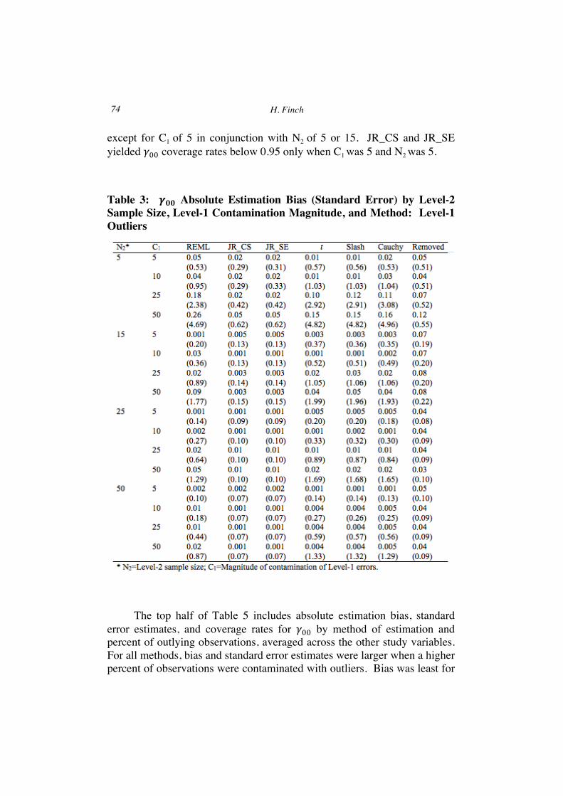
H. Finch 74
except for C1 of 5 in conjunction with N2 of 5 or 15. JR_CS and JR_SE yielded 𝛾!! coverage rates below 0.95 only when C1 was 5 and N2 was 5.
Table 3: 𝜸𝟎𝟎 Absolute Estimation Bias (Standard Error) by Level-2 Sample Size, Level-1 Contamination Magnitude, and Method: Level-1 Outliers
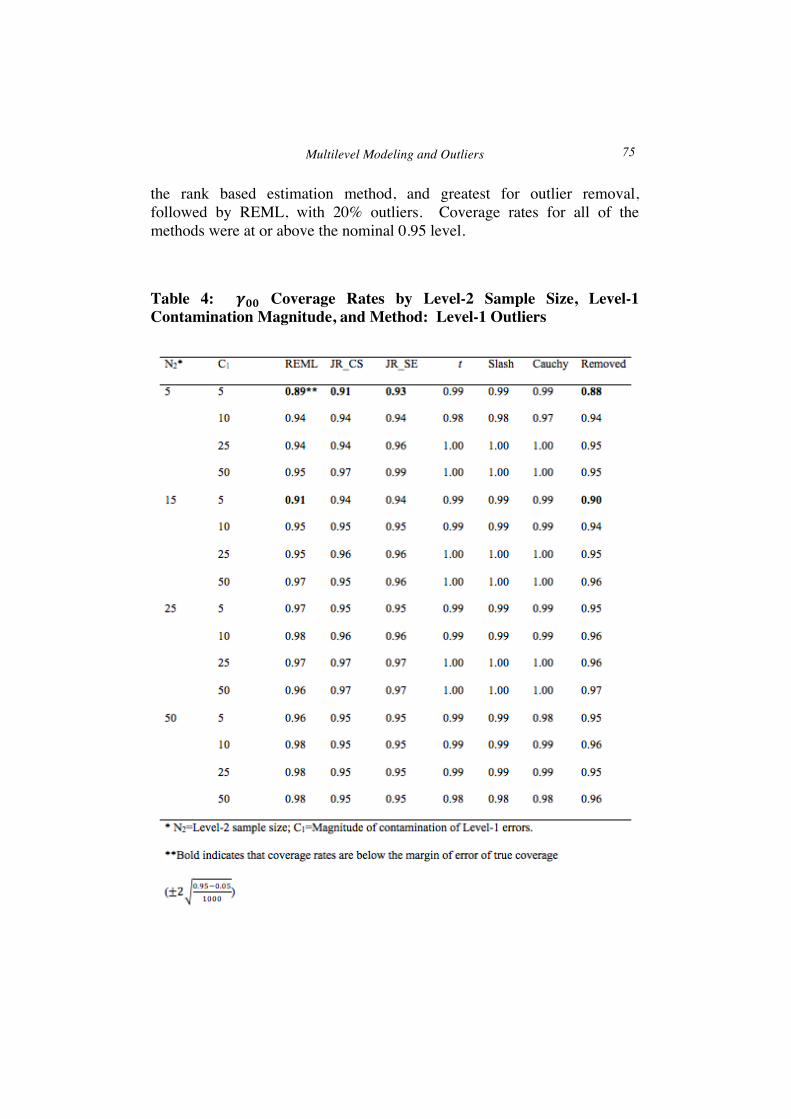
The top half of Table 5 includes absolute estimation bias, standard
error estimates, and coverage rates for 𝛾!! by method of estimation and percent of outlying observations, averaged across the other study variables. For all methods, bias and standard error estimates were larger when a higher percent of observations were contaminated with outliers. Bias was least for
Multilevel Modeling and Outliers 75
the rank based estimation method, and greatest for outlier removal, followed by REML, with 20% outliers. Coverage rates for all of the methods were at or above the nominal 0.95 level.
Table 4: 𝜸𝟎𝟎 Coverage Rates by Level-2 Sample Size, Level-1 Contamination Magnitude, and Method: Level-1 Outliers
H. Finch 76
Table 5: 𝜸𝟎𝟎 and 𝜷𝟏 Absolute Estimation Bias (Standard Error), and Coverage Rates by Percentage of Outlying Observations and Method of Parameter Estimation: Level 1 Outliers
Multilevel Modeling and Outliers 77
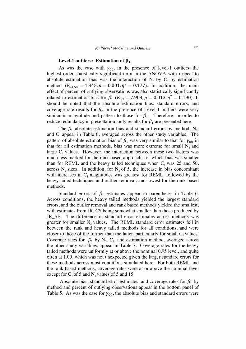
Level-1 outliers: Estimation of 𝛃𝟏 As was the case with 𝛾!!, in the presence of level-1 outliers, the
highest order statistically significant term in the ANOVA with respect to absolute estimation bias was the interaction of N2 by C1 by estimation method (𝐹!",!" = 1.845,𝑝 = 0.001, 𝜂! = 0.177). In addition, the main effect of percent of outlying observations was also statistically significantly related to estimation bias for 𝛽! (𝐹!,! = 7.904,𝑝 = 0.013, 𝜂! = 0.190). It should be noted that the absolute estimation bias, standard errors, and coverage rate results for 𝛽! in the presence of Level-1 outliers were very similar in magnitude and pattern to those for 𝛽!. Therefore, in order to reduce redundancy in presentation, only results for 𝛽! are presented here.
The 𝛽! absolute estimation bias and standard errors by method, N2, and C1 appear in Table 6, averaged across the other study variables. The pattern of absolute estimation bias of 𝛽! was very similar to that for 𝛾!! in that for all estimation methods, bias was more extreme for small N2 and large C1 values. However, the interaction between these two factors was much less marked for the rank based approach, for which bias was smaller than for REML and the heavy tailed techniques when C1 was 25 and 50, across N2 sizes. In addition, for N2 of 5, the increase in bias concomitant with increases in C1 magnitudes was greatest for REML, followed by the heavy tailed techniques and outlier removal, and lowest for the rank based methods.
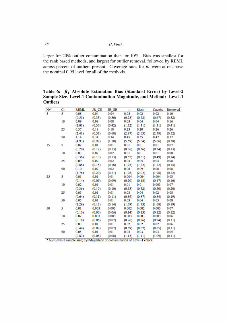
Standard errors of 𝛽! estimates appear in parentheses in Table 6. Across conditions, the heavy tailed methods yielded the largest standard errors, and the outlier removal and rank based methods yielded the smallest, with estimates from JR_CS being somewhat smaller than those produced by JR_SE. The difference in standard error estimates across methods was greater for smaller N2 values. The REML standard error estimates fell in between the rank and heavy tailed methods for all conditions, and were closer to those of the former than the latter, particularly for small C1 values. Coverage rates for 𝛽! by N2, C1, and estimation method, averaged across the other study variables, appear in Table 7. Coverage rates for the heavy tailed methods were uniformly at or above the nominal 0.95 level, and quite often at 1.00, which was not unexpected given the larger standard errors for these methods across most conditions simulated here. For both REML and the rank based methods, coverage rates were at or above the nominal level except for C1 of 5 and N2 values of 5 and 15.
Absolute bias, standard error estimates, and coverage rates for 𝛽! by method and percent of outlying observations appear in the bottom panel of Table 5. As was the case for 𝛾!!, the absolute bias and standard errors were
H. Finch 78
larger for 20% outlier contamination than for 10%. Bias was smallest for the rank based methods, and largest for outlier removal, followed by REML across percent of outliers present. Coverage rates for 𝛽! were at or above the nominal 0.95 level for all of the methods.
Table 6: 𝜷𝟏 Absolute Estimation Bias (Standard Error) by Level-2 Sample Size, Level-1 Contamination Magnitude, and Method: Level-1 Outliers
Multilevel Modeling and Outliers 79
Table 7: 𝜷𝟏 Coverage Rates by Level-2 Sample Size, Level-1 Contamination Magnitude, and Method: Level-1 Outliers
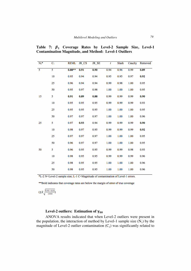
Level-2 outliers: Estimation of 𝛄𝟎𝟎 ANOVA results indicated that when Level-2 outliers were present in
the population, the interaction of method by Level-1 sample size (N1) by the magnitude of Level-2 outlier contamination (C2) was significantly related to
H. Finch 80
𝛾!! absolute estimation bias (𝐹!",!" = 1.455,𝑝 = 0.033, 𝜂! = 0.133), as was the main effect of percent of outlying observations (𝐹!,! = 5.888,𝑝 =0.028, 𝜂! = 0.165). Table 8 contains absolute estimation bias and standard errors for 𝛾!!, averaged across the other study variables. When C2 was 5, the least absolute estimation bias was present for the heavy tailed approaches, across levels of N1, whereas the greatest bias was associated with the outlier removal approach. For N1 of 5 and C2 of 25 or 50, the outlier removal approach was not able to yield estimates at all, due to a lack of convergence for the model estimator. In addition, the increase in bias concomitant with increases in C2 was greater for REML than for the other methods. The rank based approach yielded lower bias than the heavy tailed when C2 was 25 or 50, except when N1 was 5, in which case they were comparable to one another. On the other hand, for lower outlier contamination the heavy tailed methods generally yielded less biased estimates than the rank based approach.
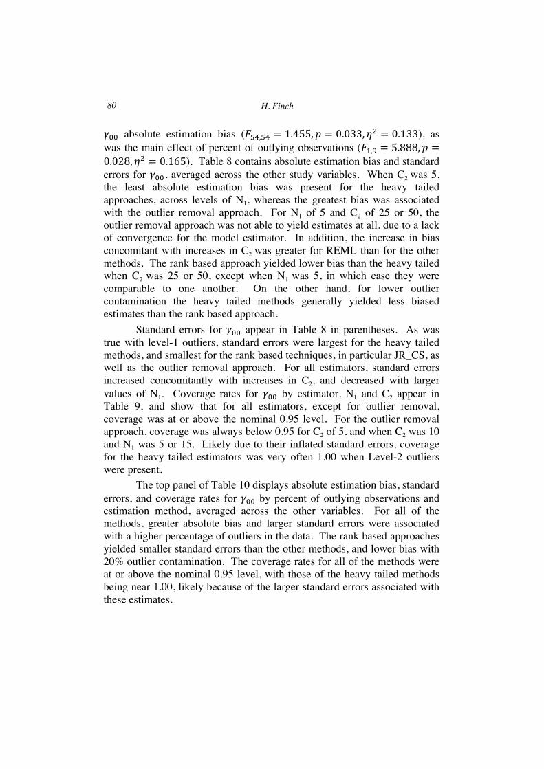
Standard errors for 𝛾!! appear in Table 8 in parentheses. As was true with level-1 outliers, standard errors were largest for the heavy tailed methods, and smallest for the rank based techniques, in particular JR_CS, as well as the outlier removal approach. For all estimators, standard errors increased concomitantly with increases in C2, and decreased with larger values of N1. Coverage rates for 𝛾!! by estimator, N1 and C2 appear in Table 9, and show that for all estimators, except for outlier removal, coverage was at or above the nominal 0.95 level. For the outlier removal approach, coverage was always below 0.95 for C2 of 5, and when C2 was 10 and N1 was 5 or 15. Likely due to their inflated standard errors, coverage for the heavy tailed estimators was very often 1.00 when Level-2 outliers were present.
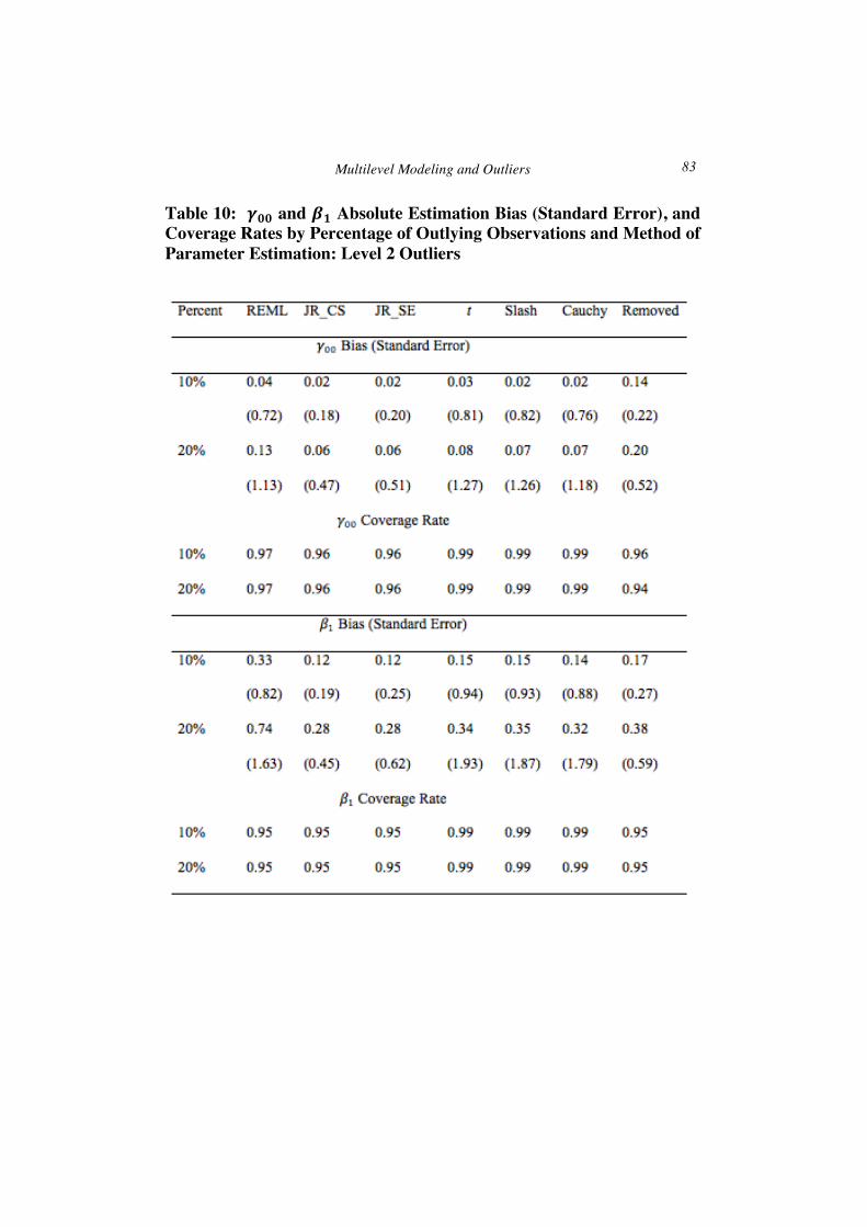
The top panel of Table 10 displays absolute estimation bias, standard errors, and coverage rates for 𝛾!! by percent of outlying observations and estimation method, averaged across the other variables. For all of the methods, greater absolute bias and larger standard errors were associated with a higher percentage of outliers in the data. The rank based approaches yielded smaller standard errors than the other methods, and lower bias with 20% outlier contamination. The coverage rates for all of the methods were at or above the nominal 0.95 level, with those of the heavy tailed methods being near 1.00, likely because of the larger standard errors associated with these estimates.
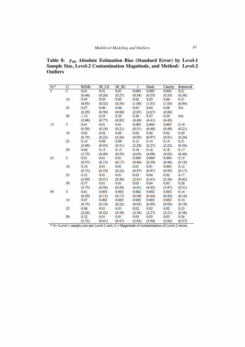
Multilevel Modeling and Outliers 81
Table 8: 𝜸𝟎𝟎 Absolute Estimation Bias (Standard Error) by Level-1 Sample Size, Level-2 Contamination Magnitude, and Method: Level-2 Outliers
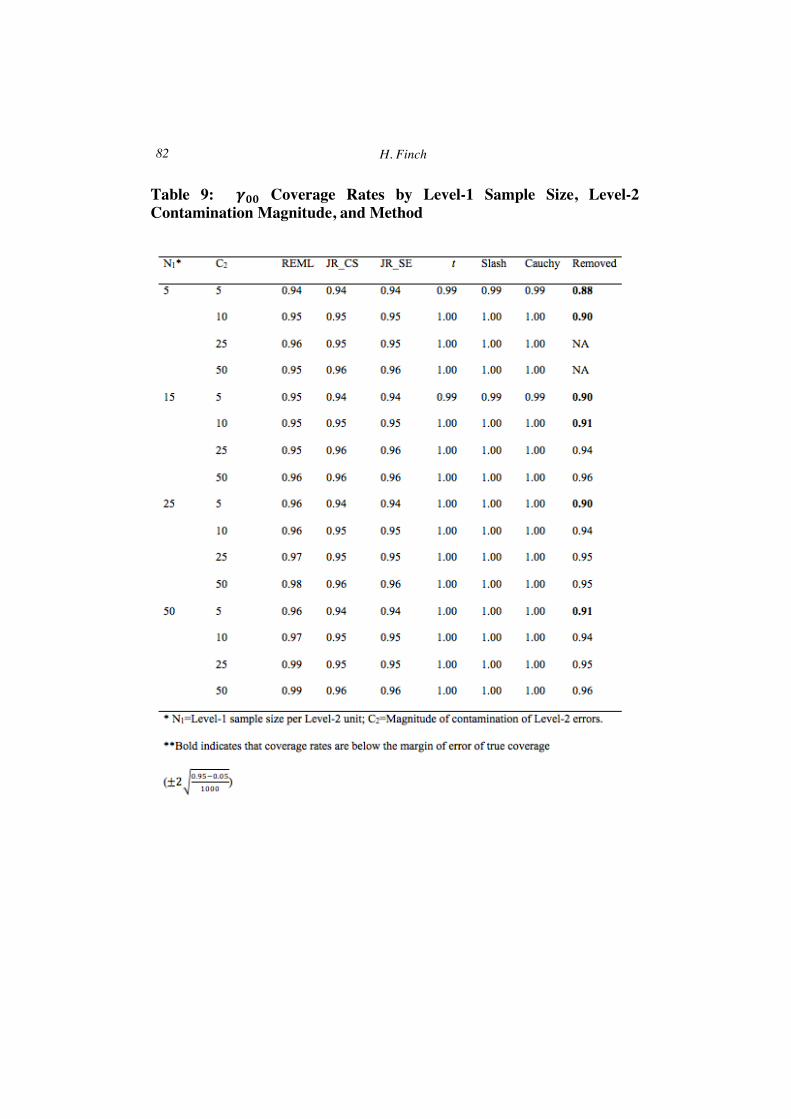
H. Finch 82
Table 9: 𝜸𝟎𝟎 Coverage Rates by Level-1 Sample Size, Level-2 Contamination Magnitude, and Method
Multilevel Modeling and Outliers 83
Table 10: 𝜸𝟎𝟎 and 𝜷𝟏 Absolute Estimation Bias (Standard Error), and Coverage Rates by Percentage of Outlying Observations and Method of Parameter Estimation: Level 2 Outliers
H. Finch 84
Level-2 outliers: Estimation of 𝛃𝟏 ANOVA revealed that the interaction of ICC by C2was statistically
significantly related to absolute estimation bias of 𝛽! (𝐹!,!" = 1.699,𝑝 =0.001, 𝜂! = 0.212), as was the main effect of percent of outlying observations (𝐹!,! = 7.002,𝑝 = 0.018, 𝜂! = 0.176). Results for 𝛽! were very similar to those for 𝛽!, and therefore only results for 𝛽! are presented here in order to save space. Estimation bias by ICC, C2, and estimation method appear in Table 11, averaged across the other variables. Across estimation methods, 𝛽! absolute estimation bias was larger in the presence of higher C2 values. In addition, bias was most pronounced for REML regardless of ICC and C2, and was comparable for the rank based and three heavy tailed estimation methods when the ICC was 0.10. However, when the ICC was 0.25, bias for the rank estimators was lower than for the heavy tailed methods at the two largest C2 values. Across most conditions, bias for the outlier removal approach was lower than that of REML, but greater than for the other methods studied here.
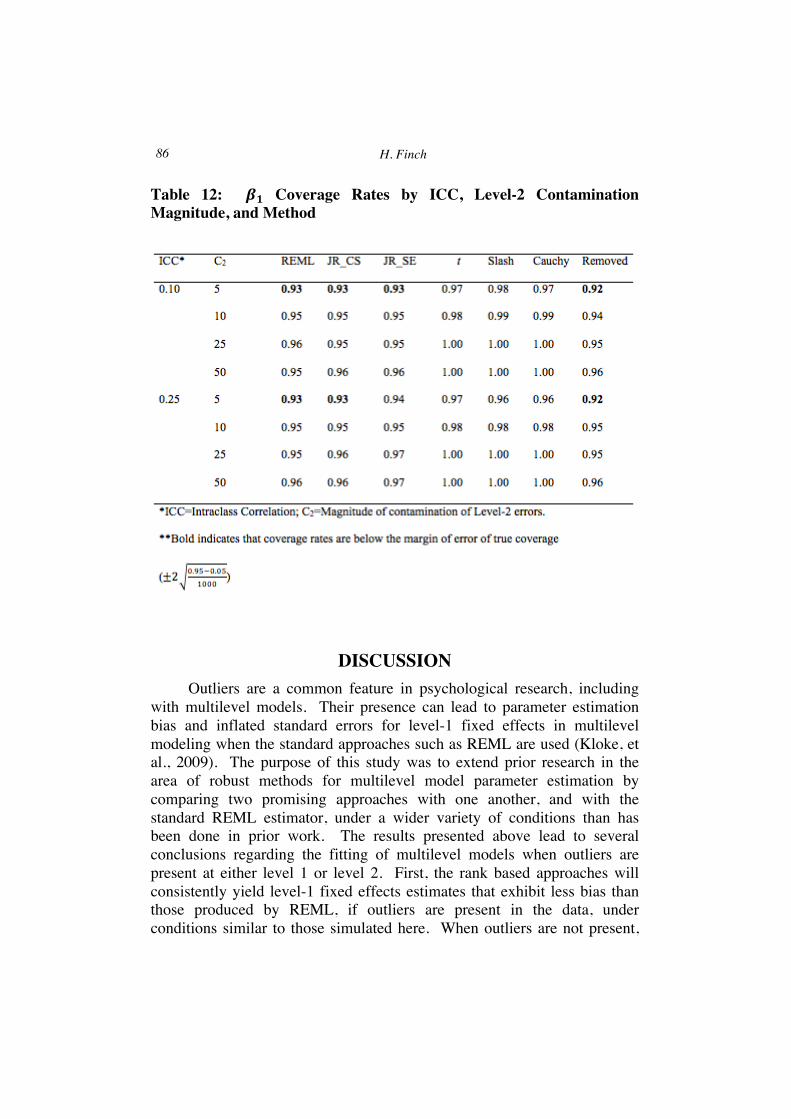
Standard errors by ICC and C2 appear in parentheses in Table 11. JR_CS and the outlier removal approach yielded the lowest standard errors across all conditions, followed by JR_SE. The largest standard errors were associated with the heavy tailed estimation methods, with the Cauchy producing somewhat smaller values than the other heavy tailed approaches. For all estimators, standard errors increased concomitantly with increases in C2. Coverage rates for 𝛽! by ICC and C2 appear in Table 12, averaged across the other study variables. For REML and the rank based methods, 𝛽! coverage rates were just below (0.93) to slightly above the nominal 0.95 level, across values of the ICC and the C2 values. The heavy tailed methods produced coverage rates above the 0.95 level, likely due to the larger standard errors associated with these methods. Outlier removal led to the lowest coverage rates for C2 of 5, regardless of the ICC.
The absolute bias, standard errors, and coverage rates for 𝛽! by the percentage of outlying observations and method of estimation for level-2 outliers are presented in the bottom panel of Table 10. As was true with other results presented above, the estimation bias and standard errors were larger for all methods with a larger percentage of outlying data, and coverage rates were at or above the nominal 0.95 level. The rank based methods yielded slightly less biased estimates than did the heavy tailed approaches, and the REML estimates displayed the greatest bias. Removing outliers resulted in more biased estimates of 𝛽! than was the case for either the rank or heavy tailed methods, but less bias than for REML. The standard errors associated with the heavy tailed methods were the
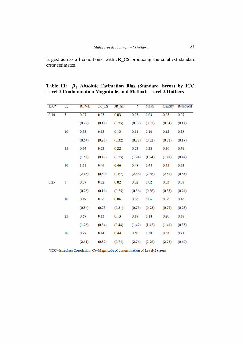
Multilevel Modeling and Outliers 85
largest across all conditions, with JR_CS producing the smallest standard error estimates.
Table 11: 𝜷𝟏 Absolute Estimation Bias (Standard Error) by ICC, Level-2 Contamination Magnitude, and Method: Level-2 Outliers
H. Finch 86
Table 12: 𝜷𝟏 Coverage Rates by ICC, Level-2 Contamination Magnitude, and Method
DISCUSSION Outliers are a common feature in psychological research, including
with multilevel models. Their presence can lead to parameter estimation bias and inflated standard errors for level-1 fixed effects in multilevel modeling when the standard approaches such as REML are used (Kloke, et al., 2009). The purpose of this study was to extend prior research in the area of robust methods for multilevel model parameter estimation by comparing two promising approaches with one another, and with the standard REML estimator, under a wider variety of conditions than has been done in prior work. The results presented above lead to several conclusions regarding the fitting of multilevel models when outliers are present at either level 1 or level 2. First, the rank based approaches will consistently yield level-1 fixed effects estimates that exhibit less bias than those produced by REML, if outliers are present in the data, under conditions similar to those simulated here. When outliers are not present,
Multilevel Modeling and Outliers 87
the rank based methods work as well as REML, producing estimates with little bias. The heavy tailed methods studied here also generally produce estimates of the level-1 fixed effects with less bias than REML estimates when outliers are present at either level and indeed, in many instances they exhibited less bias than did the rank based approach, as well. On the other hand, the heavy tailed estimators were also characterized by much larger standard error estimates than the rank based methods. These larger standard errors were in evidence across all simulated conditions, including when no outliers were present, but were most marked with greater levels of outlier contamination either in the form of a higher percentage of outliers, or when the magnitude of the outlying values was larger. Among all of the methods, JR_CS had the lowest standard errors in most cases, followed by JR_SE. Regardless of any other conditions, all of the methods exhibited coverage rates at or above the nominal 0.95 level used here, except for the REML and rank based methods when the level of contamination and the sample sizes were both small. Removing outliers from the dataset generally appears to result in more biased estimates than using one of the alternative estimators, such as the rank or heavy tailed approaches. In addition, when outliers appear at level-2, convergence of the estimators may not be possible when the level-1 sample size is small and contamination at level-2 is large.
One result of some interest is the pattern of somewhat larger standard errors for the heavy tailed than the rank based procedures, even though estimation bias is often quite similar. One possible explanation for this result is that, as noted by Pinheiro, et al. (2001), the estimation of asymptotic standard errors and confidence intervals for the fixed effects involves using MLE under the assumption that in the population the fixed effects follow a multivariate normal distribution, with variance equal to the Fisher information matrix of the marginal log-likelihood of the estimates. However, in the presence of outliers, this assumption may not be tenable, particularly as the magnitude of the outliers increases, resulting in a distortion of the distribution of the fixed effects. While speculative at this point, this hypothesis does match with the results described above, in which the standard errors of the heavy tailed fixed effects estimates increased in value concomitantly with a greater magnitude of the outlying observations. Clearly more research into this question is needed. In addition, the positive performance of the rank based methods in terms of both low bias and small standard errors, would suggest that by retaining the order of dependent variable values but not the relative magnitudes, ranking serves to greatly diminish the impact of outliers leading to low estimation bias, and relatively small standard errors.
H. Finch 88
Study limitations and directions for future research As with any study, the current work has limitations that must be
acknowledged, and which should lead to future work in this area. First, the conditions simulated here are a subset of all that could be examined. In particular, only two ICC values were included in the simulation, as were only two levels for percent of contamination. Future work should expand upon these in order to determine whether higher values of either would lead to substantive differences in the pattern of performance exhibited in this study. Second, the focus of the current work was on estimation of fixed effects. This decision was made both because researchers using multilevel models are most frequently interested in the fixed effects estimates, and because the methods examined here, particularly those based on ranks, do not produce readily reviewable output for the random effects. Nonetheless, future work needs to include estimation of random effects because they are of substantive interest in some studies, so that researchers need to know both the impact of outliers on their estimation, and the relative performance of the robust approaches in estimating them. In addition, estimation of level-2 fixed effects should also be undertaken in order to determine the impact of outliers on each of the estimation methods. With regard to the standard errors of the heavy tailed estimators, it might be beneficial to explore other methods for estimating them, such as the bootstrap. Given their inflated standard errors, coupled with the relatively low bias of the heavy tailed methods, an alternative standard error estimation technique might be of particular interest for these approaches, making them a more viable alternative for researchers to use in practice. Furthermore, future research should include an examination of parameter estimation for random slopes models. Finally, while not viewed as a limitation, it is acknowledged that the larger outlier magnitude values (e.g. 25 and 50) do represent extreme cases. They were included in the current study both because in some instances such extreme outliers may be present in the data, and also because a goal of this research was to determine how well the various methods performed at the bounds of what might be seen in practice.
Conclusions Researchers using MLMs must be cognizant of estimation problems
caused by outliers at levels-1 and 2. It is hoped that this study will help them select appropriate methods for use when outliers are present with multilevel data, thereby leading to improved data analysis and more accurate results. Based on these results, it appears that the rank based methods may hold great promise in this regard, yielding estimates that are
Multilevel Modeling and Outliers 89
less biased than those produced by the standard REML approach in many instances, and no more biased than the heavy tailed alternatives. Even when there are not outliers, the rank approach yields estimates that exhibit very little bias, and standard errors that are comparable to those produced by REML. Further, the rank methods yield smaller standard errors than their heavy tailed counterparts, and produce coverage rates near the nominal level in most situations. Finally, all of the methods studied here, including those based on ranks, are easy to employ with the R software package. It must be noted that the conditions simulated here represent only a subset of all possible cases in which a researcher may find themselves working. For example, these results do not inform situations in which the dependent variable is highly skewed, the data are heterogeneous, or when missing data are present. Future research should focus on these conditions. Considering results of the current study, however, it is recommended that if outliers are present in the context of MLM parameter estimation under conditions similar to those simulated here, the researcher consider using the rank based estimation method.
REFERENCES Bryk, A.S. & Raudenbush, S.W. (2001). Hierarchical Linear Models: Applications and
Data Analysis Methods. Thousand Oaks, CA: Sage Publications. Finch, W.H. (2012). Distribution of Variables by Method of Outlier Detection. Frontiers
in Quantitative Psychology, 3, 1-12. Fox, J. (2016). Applied Regression Analysis and Generalized Linear Models. Thousand
Oaks, CA: Sage. French, B.F. & Finch, W.H. (2012). Extensions of Mantel-Haenszel for Multilevel DIF
Detection. Educational and Psychological Measurement, 73, 648-671. Hastings, P.D., Helm, J., Mills, R.S.L., Serbin, L.A., Stack, D.M., & Schwartzman, A.E.
(2015). Dispositional and Environmental Predictors of the Development of Internalizing Problems in Childhood: Testing a Multilevel Model. Journal of Abnormal Child Psychology, 43(5), 831-845.
Hedges, L.V. & Hedberg, E.C. (2007). Intraclass Correlation Values for Planning Group-Randomized Trials in Education. Educational Evaluation and Policy Analysis, 29(1), 60-87.
Hogg, R.V. (1974). Adaptive Robust Procedures: A Partial Review and Some Suggestions for Future Applications and Theory. Journal of the American Statistical Association, 69, 909-923.
Hogg, R.V. & Tanis, E.A. (1996). Probability and Statistical Inference. New York: Prentice Hall.
Jaekel, L.A. (1972). Estimating Regression Coefficients by Minimizing the Dispersion of Residuals. Annals of Mathematical Statistics, 43, 1449-1458.
Jedidi, K. & Ansari, A. (2001) Bayesian Structural Equation Models for Multilevel Data. Invited Chapter in New Developments and Techniques in Structural Equation
H. Finch 90
Modeling Edited By George A. Marcoulides and Randall E. Schumacker, Lawrence Erlbaum Associates, Inc, NJ.
Kivlighan, D.M., Coco, G.L., & Gullo, S. (2015). Is There a Group Effect? It Depends on How You Ask the Question: Intraclass Correlations for California Psychotherapy Alliance Scale-Group Items. Journal of Counseling Psychology, 62(1), 73-78.
Kloke, J. & McKean, J.W. (2013). Small Sample Properties of JR Estimators. Paper presented at the annual meeting of the American Statistical Association, Montreal, QC, August.
Kloke, J.D., McKean, J.W., & Rashid, M. (2009). Rank-Baseed Estimation and Associated Inferences for Linear Models with Cluster Correlated Errors. Journal of the American Statistical Association, 104, 384-390.
Kreft, I.G.G. & de Leeuw, J. (1998). Introducing Multilevel Modeling. Thousand Oaks, CA: Sage.
Lange, K.L., Little, R.J.A., & Taylor, J.M.G. (1989). Robust Statistical Modeling using the t Distribution. Journal of the American Statistical Association, 84, 881-896.
Lindstrom, M.J. & Bates, D.M. (1988). Newton-Raphson and EM Algorithms for Linear Mixed-Effects Models for Repeated-Measures Data. Journal of the American Statistical Association, 83,1014-1022.
Maas, C.J.M. & Hox, J.J. (2005). Sufficient Sample Sizes for Multilevel Modeling. Methodology, 1, 127-137.
Osborne, J.W. & Overbay, A. (2008). Best Practices in Data Cleaning: How Outliers and “Fringeliers” can Increase Error Rates and Decrease the Quality and Precision of your Results. In Osborne, J.W. (Ed.). Best Practices in Quantitative Methods. Thousand Oaks, CA: Sage.
Paxton, P., Curran, P.J., Bollen, K.A., Kirby, J., & Chen, F. (2001). Monte Carlo Experiments: Design and Implementation. Structural Equation Modeling, 8, 287-312.
Pinheiro, J., Liu, C., & Wu, Y.N. (2001). Efficient Algorithms for Robust Estimation in Linear Mixed-Effects Models using the Multivariate-t Distribution. Journal of Computational and Graphical Statistics, 10, 249-276.
Qian, X., Ticha, R., Larson, S.A., Stancliffe, R.J., & Wuorio, A. (2015). The Impact of Individual and Organisational Factors on Engagement of Individuals with Intellectual Disability Living in Community Group Homes: A Multilevel Model. Journal of Intellectual Disability Research, 59(6), 493-505.
R Core Development Team. (2015). R: A Language and Environment for Statistical Computing. Vienna, Austria: R Foundation for Statistical Computing.
Rogers, W.H. & Tukey, J.W. (1972). Understanding some Long-Tailed Symmetrical Distributions. Statistica Neerlandica, 26(3), 211-226.
Seltzer, M. & Choi, K. (2003). Sensitivity Analysis for Hierarchical Models: Down Weighting and Identifying Extreme Cases using the t-distribution. In S.P. Reise and N. Duan (Eds.). Multilevel Modeling Methodological Advances, Issues and Applications. London: Lawrence Erlbaum Associates, Publishers.
Simons, J.S., Wills, T.A., & Neal, D.J. (2014). The Many Faces of Affect: A Multilevel Model of Drinking Frequency/Quantity and Alcohol Dependence Symptoms among Young Adults. Journal of Abnormal Psychology, 123(3), 676-694.
Snijders, T.A.B. & Bosker, R.J. (2012). Multilevel Analysis: An Introduction to Basic and Advanced Multilevel Modeling. London: Sage Publications.
Multilevel Modeling and Outliers 91
Song, P. X-K., Zhang, P., & Qu, A. (2007). Maximum Likelihood Inference in Robust linear Mixed-Effects Models using Multivariate t Distributions. Statistica Sinica, 17, 929-943.
Staudenmayer, J., Lake, E.E., & Wand, M.P. (2009). Robustness for General Design Mixed Models using the t-distribution. Statistical Modeling, 9, 235-255.
Thompson, D.M., Fernald, D.H., & Mold, J.W. (2012). Intraclass Correlation Coefficients Typical of Cluster-Randomized Studies; Estimates from the Robert Wood Johnson Prescription for Health Projects. Annals of Family Medicine, 10(3), 235-240.
Tong, X. & Zhang, Z. (2012). Diagnostics of Robust Growth Curve Modeling using Student’s t Distribution. Multivariate Behavioral Research, 47(4), 493-518.
Wang, J. & Genton, M.G. (2006). The Multivariate Skew-Slash Distribution. Journal of Statistical Planning and Inference, 136, 209-220.
Welsh, A.H. & Richardson, A.M. (1997). Approaches to the Robust Estimation of Mixed Models. In G. Maddala and C.R. Rao (Eds.), Handbook of Statistics, Vol 15, pp. 343-384. Amsterdam: Elsevier Science B.V.
Wilcoxon, F. (1945). Individual Comparisons by Ranking Methods. Biometrics Bulletin, 1(6), 80-83.
Yuan, K-H., Bentler, P.M., & Chan, W. (2004). Structural Equation Modeling with Heavy Tailed Distributions. Psychometrika, 69(3), 421-436.
Yuan, K.-H. & Bentler, P.M. (1998). Structural Equation Modeling with Robust Covariances. Sociological Methodology, 28, 363-396.
H. Finch 92
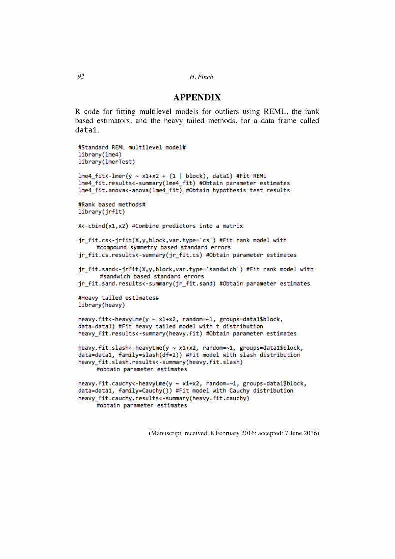
APPENDIX R code for fitting multilevel models for outliers using REML, the rank based estimators, and the heavy tailed methods, for a data frame called data1.
(Manuscript received: 8 February 2016; accepted: 7 June 2016)