Multibody dynamics simulation of geometrically exact … · 2012-08-13 · multibody dynamics...

multibody dynamics simulation of geometrically exact cosserat rods 1

Multibody dynamics simulation of geometrically exactCosserat rods

Holger Lang, Joachim Linn, Martin Arnold♯

Fraunhofer Institute for Industrial MathematicsFraunhofer Platz 1, 67663 Kaiserslautern, Germany

[email protected], [email protected],

♯ Institute for Mathematics, Martin-Luther-Universitat Halle-Wittenberg06099 Halle (Saale), Germany

[email protected]

Abstract

In this paper, we present a viscoelastic rod model that is suitable for fast and accurate dynamicsimulations. It is based on Cosserat’s geometrically exact theory of rods and is able to representextension, shearing (‘stiff’ dof), bending and torsion (‘soft’ dof). For inner dissipation, a consistentdamping potential proposed by Antman is chosen. We parametrise the rotational dof by unit quater-nions and directly use the quaternionic evolution differential equation for the discretisation of theCosserat rod curvature.

The discrete version of our rod model is obtained via a finite difference discretisation on a staggeredgrid. After an index reduction from three to zero, the right-hand side function f and the Jacobian∂f/∂(q, v, t) of the dynamical system q = v, v = f(q, v, t) is free of higher algebraic (e. g. root)or transcendental (e. g. trigonometric or exponential) functions and therefore cheap to evaluate. Acomparison with Abaqus finite element results demonstrates the correct mechanical behaviour of ourdiscrete rod model. For the time integration of the system, we use well established stiff solvers likeRadau5 or Daspk. As our model yields computational times within milliseconds, it is suitable forinteractive applications in ‘virtual reality’ as well as for multibody dynamics simulation.

Keywords. Flexible multibody dynamics, Large deformations, Finite rotations, Constrained mechanical systems,

Structural dynamics.

1 Introduction

For rods — i. e. slender one dimensional flexible structures — the overall deformation as response tomoderate external loads may become large, although locally the stresses and strains remain small. TheCosserat rod model [1, 3, 61, 62] is an appropriate model for the geometrically exact simulation ofdeformable rods in space (statics) or space-time (quasistatics or dynamics). A Cosserat rod can beconsidered as the geometrically nonlinear generalisation of a Timoshenko-Reissner beam. In contrast to aKirchhoff rod, which can be considered as a geometrically nonlinear generalisation of an Euler-Bernoullibeam, a Cosserat rod allows to model not only bending and torsion — these are ‘soft dof’ —, but as wellextension and shearing — these are ‘stiff dof’.This article is concerned with a discrete finite difference (FD) Cosserat rod model that is firmly based onstructural mechanics and applicable to compute dynamical deformations of rods very fast and sufficientlyaccurate. We continue the work [40, 41] presented at Eccomas 2007, which considered the fast simula-tion of geometrically exact Kirchhoff rods in the quasistatic case, and complement recent investigations[33] of discrete FD type Cosserat rods within the framework of Discrete Lagrangian Mechanics.

The paper is structured as follows: In section 2, we describe the basic equations for a Cosserat rod in thecontinuum, where we formulate the rotational dof of the rod directly in terms of unit quaternions. Ofcourse, other possibilities such as Rodriguez parameters, rotation vectors, Euler or Cardan angles, exist[6, 14, 24, 50, 56]. All of them have their pros and cons. So as a pro, gimbal locking can be avoided withquaternions. A con is that they must be kept at unity length.In section 3, we present our discrete numerical model of the Cosserat rod, based on finite differences. Incontrast to a displacement based discretisation by the finite element method (FEM), where the primary

2 multibody dynamics simulation of geometrically exact cosserat rods

unknowns are situated at the nodes (= vertices), we suggest a discretisation on a staggered grid. Thismeans that the translatory resp. the rotatory dof are ordered in an alternating fashion and that thetrapezoidal resp. midpoint quadrature formulas form the basis for the approximation of the internalenergy integrals.This construction allows to interpret the discrete Cosserat rod as a sequence of (almost) rigid cylinderswith the primary rotatory dof situated at the cylinder centers of mass. Likewise, the discretised energyterms may be interpreted as bushings which connect the rigid body dof of adjacent cylinders by appropri-ate springs and dampers. Here the parameters of these ‘springs’ and ‘dampers’ are rigorously derived fromthe continuous Cosserat strain and curvature relations. Whereas the extensional and shearing strains,which belong to such cylinders, are discretised via finite differences in the one and only one canonicalstandard fashion, several choices for the discrete bending and torsion curvature measures are possible.These curvatures belong to the vertices between the cylinders and result from various possible rotationinterpolations of varying accuracy and computational costs.We formulate the final discrete model as a constrained mechanical system, resulting in the well knownLagrangian DAE system of index three. Index reduction to zero plus introduction of Baumgarte penaltyaccelerations yields a universal ODE formulation, suitable for any ODE solver. As an alternative tothe Baumgarte method, stabilisation by projection is as well convenient and cheap. For our approach,the inverse mass-constraint matrix is explicitly known, and multiplication with the latter is exactly asexpensive as multiplication with the mass-constraint matrix itself. The model can be implemented usingalgebraic expressions free of trigonometric and square root functions, which permits extremely cheapright hand side function and Jacobian evaluations. Moreover, both extensible and inextensible Kirchhoffrod models can be conveniently fed into this framework as well.In section 4, we present accurate numerical results, compared to Abaqus FE solutions. In view of appli-cations in robotics and assembly simulation as well as interactive deformations of flexible 1D structuresin virtual reality environments we are especially interested in moderately fast motions dominated ratherby the internal forces and moments associated to bending and twisting than inertial effects. In such caseswe propose to impose strong damping on extension and shearing, which are of subordinate importance,and to solve the resulting stiff system via well established methods [28, 29, 49]. As our model allowsfor accurate computations within milliseconds, it is likewise adequate for multibody dynamics simulations.

Where can this work be situated within the state of the art rod models?The handling of flexible objects in multibody dynamics simulations has been a long term field ofresearch until today [10, 11, 14, 54, 57, 58, 60]. The classical approach in industrial applications, whichis supported by today’s commercial software packages such as SimPack, Adams or VirtualLab, rep-resents flexible structures by vibrational modes, e. g. of Craig /Bampton type [18, 19], that are obtainedfrom numerical modal analysis within the range of linear elasticity. Such methods are suitable andaccurate to represent oscillatory response that results from linear response of the flexible structure.Unlike that, our approach is not of modal kind, but based on a geometrically nonlinear structural model.However, our method of discretisation contrasts the usual one in computational continuum mechanics,where the finite element approach is favored [10, 11, 13, 14, 20, 31, 32, 61, 62] due to its generalapplicability for arbitrarily complex geometries. While the geometrical complexity of 2D and 3D domainsoften implies practical limitations for the applicability of the conceptually simple FD approach, this isnot the case for the 1D domain of a rod model.A general problem in geometrically nonlinear FE is the proper interpolation of the finite rotations [7,20, 52] such that objectivity of the strain measures is maintained, i. e. invariance under rigid bodymotions. In multibody dynamics, this problem is successfully addressed by the absolute nodal coordinateformulation (ANCF) [57, 58].However, especially FE of higher order require sophisticated and technically intricate interpolation pro-cedures that lead to models with expensive right hand side functions and Jacobians. In contrast tothese rather general approaches, the finite difference based method being presented below is tailored tononlinear rod models resulting in a very straightforward solution scheme that maintains objectivity byconstruction.Our approach is inspired by FD type discretisations of inextensible Kirchhoff rods using insights fromDiscrete Differential Geometry (DDG) [8, 12]. The comparison to physical experiments shown in [8]


demonstrate that such discretisation techniques yield a physically correct model behaviour even at verycoarse discretisations. We refer to [33] for a brief discussion of the DDG aspects for a FD type discretisa-tion of the strain measure of Cosserat rods and its relation to low order FE using piecewise linear shapefunctions.

2 Geometrically exact Cosserat rods in the continuum

Our starting point for the continuous Cosserat rod model is Simo’s exposition [61, 62] of the modelproposed earlier by Antman and Reissner [1, 51]. For the constitutive material behaviour, we choosea simple linear viscoelastic one [2, 3]. The elastic parameters can be straightforwardly deduced frommaterial and geometric parameters [42]. Concerning the damping model, we note that it is macroscopicand phenomenological, it comprises not only pure material damping, but also miscellaneous dampingmechanisms. We assume both the elastic and viscoelastic parts as diagonal. The generalisation to non-diagonal, symmetric and positively definite constitutive Hookean tensors or to nonlinear hyperelasticmaterials is straightforward. We concentrate on the description of the internal potential, dissipation andkinetic energies in sections 2.1, 2.2 and 2.3 respectively, as these will be the basis for the discrete modellater. In section 2.4 we give a detailed exposition of the dynamic equations of motion with the rotatorypart formulated in terms of quaternions.We start with the kinematics for the Cosserat rod. The Cosserat rod is completely determined by itscenterline of mass centroids

x : [0, L] × [0, T ] → R3, (s, t) 7→ x(s, t)

and its unit quaternion field

p : [0, L] × [0, T ] → S3 = ∂BH

1 (0) → H, (s, t) 7→ p(s, t),

see also [21, 39]. For our purposes, the set of unit quaternions S3 = ∂BH

1 (0) = p ∈ H : ‖p‖ = 1 ⊂ H,which is a subgroup of the multiplicative quaternionic group H, provides a convenient representationof — non-commutative — spatial rotations of orthonormal frames, which are elements of the groupSO(3) = Q ∈ R3×3 : QQ⊤ = Q⊤Q = I, detQ = 1. The quaternion field uniquely determines itsorthonormal frame field

R p : [0, L]× [0, T ]p−→ S

3 = ∂BH

1 (0)R−→ SO(3), (s, t) 7→ R

(

p(s, t))

.

The situation is depicted in Figure 1. Any point of the deformed rod in space s and time t is addressedby the map [0, L] × [0, T ] × A ∋ (s, t, (ξ1, ξ2)) 7→ x(s, t) + ξ1d

1(p(s, t)) + ξ2d2(p(s, t)). The parameter

s ∈ [0, L] is the arc length of the undeformed rod centerline, where L > 0 is the total arc length ofthe undeformed centerline and A ⊂ R2 is a bounded, connected coordinate domain for the coordinates(ξ1, ξ2) in the cross section, which is assumed to remain rigid and plane throughout the deformation. Inclassical differential geometry, the object (x(·, t), (R p)(·, t)) constitutes a so-called ‘framed curve’. Fora quaternion p = p0 + p = ℜ(p) + ℑ(p) = (p0; p1, p2, p3)

⊤ ∈ H the frame R(p) is given by the Euler map

R : H → RSO(3), p 7→ R(p) =(

d1(p) | d2(p) | d3(p))

=(

2p20 − ‖p‖2

)

I + 2p ⊗ p + 2p0E(p) (1)

with the alternating skew tensor E , which identifies skew tensors in so(3) with their corresponding axialvectors in R3 via

E : R3 = ℑ(H) → so(3), E(u) =

0 −u3 u2

u3 0 −u1

−u2 u1 0

, E(u)v = u × v for u, v ∈ R3.

We write u ≃ E(u) for u ∈ R3. It is convenient to identify ℑ(H) = R3, i. e. vectors are treated as purelyimaginary quaternions and vice versa. The directors d1(p) and d2(p) span the rigid cross section of therod. The third director d3(p) is always normal to the cross section, and its deviation from the direction


Figure 1: The kinematical quantities of a continuous Cosserat rod.

of the centerline tangent ∂sx indicates transverse shearing. As R(λp) = λ2R(p) holds for each p ∈ H andλ ∈ R, the Euler map p 7→ R(p) given by (1) is sensitive w. r. t. stretching of p. In particular, (1) mapsS3 into SO(3), where R(−p) = R(p) holds, such that p and its antipode −p describe the same rotation.Conversely for each rotation Q in SO(3) there exist exactly two unit quaternions — necessarily antipodes— that produce Q. So the unit sphere S3 covers SO(3) exactly twice [23, 25, 34] via the Euler map.Stretched rotation can be expressed via quaternions as

R(p)v = pvp (forward) and R(p)⊤v = pvp (backward) (2)

for p ∈ H and v ∈ ℑ(H) = R3, especially di(p) = peip = R(p)ei for each of the space fixed Euclidean basevectors e1, e2 and e3 (classically denoted by ‘i’, ‘j’ and ‘k’) of ℑ(H) = R3. Recall that the quaternionproduct is defined by

pq = p0q0 − 〈p, q〉 + p0q + q0p + p × q for p, q ∈ H.

We use the symbols p0 = ℜ(p) resp. p = ℑ(p) to denote the real resp. the imaginary (=vector) partand p = p0 − p to denote the conjugate of a quaternion p ∈ H. Note that p = ‖p‖2p−1, where p−1 is themultiplicative inverse of p. Thus unit quaternions yield pure rotations without stretching. For details onthe Hamilton quaternion division algebra, see [23].In summary, the configuration of a Cosserat rod is determined by six degrees of freedom, all functions ofthe material coordinate s and time t: three translatory ones x(s, t) ∈ R

3 locating the position of the crosssection centroid on the centerline of the rod in space, and three rotatory ones p(s, t) ∈ S3 which fix theorientation of the material frame within the corresponding cross section of the rod. Correspondingly, thereexist six objective strain measures which monitor the local change of these kinematical dof and determinethe rod configuration up to an overall rigid body motion. From the viewpoint of the differential geometry,these are precisely the six differential invariants of a framed curve (see ch. III on moving frames in Cartan’sbook [15]).

Remark 2.1 (Kirchhoff rod models) In the structural mechanics of rods, also the classical modelvariants of Kirchhoff and Love [22, 36, 37, 42] have received considerable interest [16, 35, 44, 45, 48].These variants may be obtained from the more general Cosserat model as described above by imposingadditional kinematical constraints on the deformed rod configuration. An ‘extensible Kirchhoff rod’additionally satisfies the pair of constraints 〈d1, ∂sx〉 = 〈d2, ∂sx〉 = 0, which inhibits transverse shearingof the rod by confining the cross sections to remain normal to the centerline tangent. This reduces thenumber of dof from six to four. An ‘inextensible Kirchhoff rod’ additionally satisfies ‖∂sx‖ = 1, which


implies that the centerline remains parametrised by arc length and inhibits longitudinal stretching (orcompression) of the rod. Combining these constraints forces the centerline tangent to coincide with thecross section normal, i. e. d3 = ∂sx, which reduces the number of dof to three.

2.1 Continuous potential energies and strain measures

The total potential energy V = VSE +VBT is additively decomposed into extensional and shearing energyVSE and bending and torsion energy VBT . In V , we include only the internal elastic energies, otherconservative forces such as the gravitational force can simply be added as additional external forces onthe right hand side of the balance equations. The potential extensional and shearing energy is givenby

VSE =1

2

∫ L

0

Γ⊤CΓΓds, CΓ =

0GA1

GA2

EA

, (3)

where the material strains are defined by

Γ = R(p)⊤∂sx − e3 = p∂sxp − e3. (4)

Γ1 resp. Γ2 are the strains corresponding to shearing in d1- resp. d2-direction, Γ3 is the strain corre-sponding to extension in d3-direction. In components, we have

Γ1 = 〈d1(p), ∂sx〉, Γ2 = 〈d2(p), ∂sx〉, Γ3 = 〈d3(p), ∂sx〉 − 1. (5)

E > 0 denotes Young’s modulus and G > 0 the shear modulus of the material, A =∫∫

Ad(ξ1, ξ2) is the

area of the rigid cross section, A1 = κ1A and A2 = κ2A are some effective cross section areas with someTimoshenko shear correction factors 0 < κ1, κ2 ≤ 1, cf. [17]. Note that Γ is a vector (= purely imaginaryquaternion) in R3, which we identify with ℑ(H). The potential bending and torsion energy is

VBT =1

2

∫ L

0

K⊤CKK ds, CK =

0EI1

EI2

GJ

, (6)

where the material curvature vector is given by

K ≃ E(K) = R(p)⊤∂sR(p). (7)

K1 resp. K2 are the curvatures corresponding to bending around the d1- resp. d2-axis, K3 is thecurvature corresponding to torsion around the d3-axis. Again, note that K ∈ R3 = ℑ(H).The ‘Darboux’ vector k = RK =

∑

j Kjdj is the spatial counterpart of the material curvature vector

and appears in the generalised Frenet equations ∂sdj = k × dj , which describe the spatial evolution of

the frame directors dj along the centerline of the rod at fixed time.The geometric moments of inertia of the rigid cross section I1 =

∫∫

Aξ22 d(ξ1, ξ2) and I2 =

∫∫

Aξ21 d(ξ1, ξ2)

and the polar moment J = I3 =∫∫

A(ξ2

1 + ξ22) d(ξ1, ξ2) = I1 + I2 encode the geometrical properties of

the cross section that enter into the stiffness constants of the potential energy (6). If the cross sectionis symmetric, then we have I1 = I2 and J = I3 = 2I1 = 2I2. The conservative elastic forces FΓ andmoments MK are derived from the potential energy as FΓ = CΓΓ = 1

2∂Γ(Γ⊤CΓΓ) and MK = CKK =12∂K(K⊤CKK). Clearly, any other more general form of hyperelastic constitutive material behaviourcould be used instead [26, 61]. If the rod possesses non-vanishing precurvature K0 : [0, L] → R3 in theundeformed configuration, K can simply be replaced by K − K0 in (6) throughout the model [61].

Remark 2.2 (Hard and soft degrees of freedom) The slenderness of a typical rod geometry is char-acterised by the smallness of the parameter ε =

√A/L which measures the ratio of the linear dimension

of the cross section to the length of a rod. As I =√

I21 + I2

2 ≃ A2, an estimate of the relative order ofmagnitude of the potential energy terms (3) and (6) yields VBT /VSE ≃ I/(AL2) ≃ ε2. This explains therelative stiffness of a rod w. r. t. shearing and extension compared to bending and twisting deformationsas a geometrical effect, independent of the material properties.


It is well known that the strain measures (4) and (7) are objective (or frame-indifferent) quantities[38, 61]. It is likewise known [25, 39] that (7) is equivalent to

K = 2p∂sp (8)

provided that the quaternion p is of unit length. Identity (8) will turn out to be especially useful later, aswe will use it to discretise the curvature directly on the level of quaternions. The geometry of S3 is usedfor interpolation purposes: Concerning rotations, cf. (1), it is completely ’isotropic’ in the sense that nospecial direction is preferred. This property will make our discrete curvature measures frame-indifferent.

2.2 Continuous dissipation energies and strain rates

Our approach to model dissipation follows [2, 3]. We choose friction forces resp. moments that areproportional to the strain rates resp. curvature rates. The total dissipation energy D = DSE + DBT

consists of dissipative extensional and shearing energy DSE plus dissipative bending and torsion energyDBT . The dissipative extensional and shearing energy is

DSE =

∫ L

0

Γ⊤CΓΓds, CΓ =

0

cΓ1

cΓ2

cΓ3

(9)

with the material strain rates Γ = ∂tR(p)⊤∂sx + R(p)⊤∂2stx. The dissipative bending and torsion

energy is given by

DBT =

∫ L

0

K⊤CKK ds, CK =

0

cK1

cK2

cK3

(10)

with the material curvature rates K ≃ ∂tE(K) = ∂tR(p)⊤∂sR(p) + R(p)⊤∂2stR(p). The nonnegative

constants cΓi and cK

i for i = 1, 2, 3 denote some viscoelastic material parameters. The dissipative damping

forces F Γ and moments M K are derived from the dissipation potential as F Γ = 2CΓΓ = ∂Γ(Γ⊤CΓΓ)

and M K = 2CKK = ∂K(K⊤CKK). Of course, any other more general form of consistent viscoelasticconstitutive material behaviour could replace these assumptions.

2.3 Continuous kinetic energies

The total kinetic energy T = TT + TR consists of two parts, the translatory TT and the rotatory TR

kinetic energy, given by

TT =A

2

∫ L

0

‖x‖2ds, TR =

2

∫ L

0

Ω⊤IΩ ds, I =

0I1

I2

J

. (11)

Here the material angular velocity vector (or the ‘vorticity’ vector) is

Ω ≃ E(Ω) = R(p)⊤∂tR(p). (12)

In (11), > 0 is the mass density per volume, I1, I2 and J = I3 are as above, and we identify Ω ≃ E(Ω).Note again that Ω ∈ R3 = ℑ(H). The kinetic energy takes on the special form (11), since it is assumedthat the rod centerline x passes through the centers of mass and the directors d1, d2 are aligned in parallelto the geometric principal directions of inertia of the cross sections [61].


We rewrite the rotatory kinetic energy with the identity Ω⊤IΩ = p⊤µ(p)p and the p dependent 4 × 4quaternion mass matrix

µ(p) = 4Q(p)IQ(p)⊤, Q(p) =

(

p0 −p⊤

p p0I + E(p)

)

=

p0 −p1 −p2 −p3

p1 p0 −p3 p2

p2 p3 p0 −p1

p3 −p2 p1 p0

(13)

Details are carried out in [9, 39, 56] and the references cited therein. In that context, Q(p) is sometimescalled the ‘quaternion matrix’ corresponding to p ∈ H, since it allows to express the product of p withanother quaternion q ∈ H as a matrix-vector product, i. e. pq = Q(p)q. The mass matrix satisfies thesymmetry property µ(−p) = µ(p), which is a consequence of the fact that both p and −p describe thesame rotation R(p) = R(−p). The kernel of µ(p) is given by kerµ(p) = Rp, consequently we have rkµ(p)equal to three. The matrix µ(p) is positively semi-definite with the one singular dimension in directionp.Similarly as for the curvature, equation (12) for the angular velocity can be rewritten directly in termsof the unit quaternion p, namely,

Ω = 2p∂tp, (14)

see [38, 63]. The reader should note that the situation for K and Ω is completely analogous from atwo dimensional field view. For our discrete model, evolution (8) is the basis for spatial discretisation.Evolution (14) is solved ‘continuously’ in time, of course.

2.4 Continuous equations of motion

It can be shown [39] that the unknowns x(s, t) and p(s, t) of a Cosserat rod, for given exterior materialforce densities F = F (t) (per length) and given exterior material moment densities M = M(t) (perlength), satisfy the following nonlinear system of partial differential-algebraic equations,

Ax = ∂s(pF p) + pF p

[

µp − 1

2∂p

(

p⊤µp)

+ ∂p

(

µp)

p

]

= 2(

x′pF + ∂s(pM) + p′M + pM)

− λp

0 = ‖p‖2 − 1

. (15)

The first equation (151) corresponds to the balance of linear momentum, the second one (152) to thebalance of angular momentum. Here ′ = ∂s, ˙ = ∂t, µ = µ(p) from (13) and λ : [0, L] × [0, T ] → R,(s, t) 7→ λ(s, t) denote some Lagrange multipliers, which must be introduced as additional unknownsbecause of the presence of the normality condition for the quaternions [39]. Together with appropriateinitial and boundary conditions, this is the system that has to be solved for the unknowns x, p and λ.

In (15), the viscoelastic forces and moments are given by F = CΓΓ + 2CΓΓ and M = CKK + 2CKKdue to the constitutive assumptions. Hence, in the undamped — purely elastic and conservative — case,the shearing forces F 1, F 2, the extensional force F 3, the bending moments M1, M2 and the torsionalmoment M3 are related to the shearing strains Γ1, Γ2, the extensional strain Γ3, the bending curvaturesK1, K2 and the torsional curvature K3 via

F 1 = GA1Γ1, F 2 = GA2Γ

2, F 3 = EAΓ3, M1 = EI1K1, M2 = EI2K

2, M3 = GJK3. (16)

Originally in [61, 62], averaging the normal Piola-Kirchhoff tractions and corresponding torques over thecross section of the deformed rod, it was shown that the Cosserat rod must satisfy the following spatialform of the balance equations of motion, namely

A x = ∂sf + f(

iω + ω × iω)

= ∂sm + ∂sx × f + m. (17)

This original formulation of the equations of motion, which is probably more familiar to the reader, canas well be found in [2, 3]. Here the spatial quantities

γ = RΓ, k = RK, ω = RΩ, i = RIR⊤, f = RF, m = RM, f = RF , m = RM (18)


are obtained from the corresponding material ones by a ‘push forward ’ rotation via R. The componentsof any of these spatial quantities in the moving coordinate system (d1, d2, d3) are identical to the compo-nents of the corresponding material quantities, measured in the fixed global coordinate system (e1, e2, e3).

It can be shown that the systems (15) and (17) are equivalent. As the reader might feel unfamiliar with(15), we briefly sketch the simplest way, how (15) can be derived from the common system (17). Thesimplest way to show this is to insert (18) into (17) in order to obtain the material form

A x = ∂s(RF ) + RF

R(

IΩ + Ω × IΩ)

= ∂s(RM) + ∂sx × (RF ) + RM(19)

from the spatial form (17) of the balance equations, to let R = R(p) with the Euler map (1) and touse the basic properties (2), the angular velocity expression (14), the hidden constraints 〈p, p〉 = 0 and〈p, p〉 = −‖p‖2 and straightforward quaternion algebra. The details are not difficult, but rather lengthy.They are carried out step-by-step in [39]. Alternatively, the quaternionic formulation (15) of the balanceequations (17) can be derived from a two-dimensional variational principle in the variable (s, t). This isnot topic of the present paper, but the interested reader is referred to [39] for a detailed exposition.

Before finishing this section, let us briefly explain, how (15) can be solved for the quaternionic accelerationp. To that end, let µ(p)♯ for p ∈ H denote the matrix

µ(p)♯ = 4Q(p)I♯Q(p)⊤, I♯ =

0

I−11

I−12

J−1

.

The matrix µ(p)♯ is ‘almost’ an inverse of the radially singular mass µ(p): Actually, it satisfies theproperty µ(p)♯µ(p) = I − p ⊗ p, this is µ(p)♯µ(p)π = π − 〈p, π〉p for each p ∈ S3 and π ∈ H. This meansthat µ♯µ extracts the tangential part of π. Now, if we left-multiply (152) with µ(p)♯, the d’Alembertconstraint forces λp at the right-hand side are eliminated, since kerµ(p)♯ = Rp. If we use the constraint〈p, p〉 = −‖p‖2 for the quaternionic normal acceleration, we end up in the system

x =1

A

(

∂s(pF p) + pF p)

p =2

µ(p)♯

(

4pI ˙pp + x′pF + ∂s(pM) + p′M + pM)

− ‖p‖2p. (20)

Here as well the helpful identity 12∂p(p

⊤µ(p)p) − ∂p(µ(p)p)p = 8pI ˙pp, see [39, 56], was used. In fact,system (20) is equivalent to (15). Hence, it is also equivalent to (17). In section 3.4, we will demonstratethat the finite difference discretisation schemes, which we propose, are consistent to (20).

3 Discrete Cosserat rods via finite differences and quotients

Here we present our discrete version of the Cosserat model. Sections 3.1, ..., 3.4 are the discrete counter-parts of sections 2.1, ..., 2.4 respectively.Contrasting the more frequently applied finite element approach (see e.g. [64]), we propose the followingstaggered grid discretisation. We subdivide the arc length interval [0, L] into N segments [sn−1, sn] withthe vertices 0 = s0 < s1 < . . . < sN−1 < sN = L. Together with the segment midpoints sn−1/2 =(sn−1 + sn)/2 we obtain the staggered grid 0 = s0 < s1/2 < s1 < . . . < sN−1 < sN−1/2 < sN = L, onwhich the various kinematical quantities of our discrete Cosserat rod model reside.We associate the discrete translatory degrees of freedom xn : [0, T ] → R

3, i. e. the cross sectioncentroids, to the vertices, x0(·) ≈ x(s0, ·), ..., xN (·) ≈ x(sN , ·), and the discrete rotatory degrees offreedom pn−1/2 : [0, T ] → H, i. e. the quaternions specifying the frame orientations, on the segmentmidpoints, p1/2(·) ≈ p(s1/2, ·), ..., pN−1/2(·) ≈ p(sN−1/2, ·), so the corresponding frames R(pn−1/2) and


directors di(pn−1/2) likewise live on the midpoints. In order that the quaternions remain in S3, we have tointroduce the discrete Lagrange multipliers λn−1/2 : [0, T ] → R, situated on the midpoints, λ1/2(·) ≈λ(s1/2, ·), ... λN−1/2(·) ≈ λ(sN−1/2, ·) and N constraints 0 = gn−1/2(q) with 2gn−1/2(q) = ‖pn−1/2‖2−1,which are situated here as well.A staggered grid discretisation using quaternionic dof was already proposed in [21] for the case of aninextensible Kirchhoff rod formulated as a Hamiltonian system. We extend this idea to shearable andextensible Cosserat rods in the Lagrangian setting. Due to the relative stiffness of the extensional andshearing dof (cf. remark 2.2), the staggered grid approach permits an interpretation of the rod as asequence of almost rigid cylinders, connected with appropriate ‘bushings’ for bending and torsion. Weconsequently use the notation ·n for quantities at the vertices sn; here n ranges from 0 to N . We use thenotation ·n−1/2 for quantities that are situated on the midpoints sn−1/2; here n ranges from 1 to N , ifnot otherwise explicitly stated. The situation is depicted in Figure 2.In the sequel, we discretise the continuous internal Cosserat energy integrals V , T and D by the use ofeither midpoint or trapezoidal quadrature, depending on where which quantity ist ‘at home’. The weightfactors for the midpoint rule are the segment lengths ∆sn−1/2 = sn − sn−1. Likewise, the weights for thetrapezoidal rule are the lengths of the bucked segments 2δs0 = ∆s1/2, 2δsn = ∆sn−1/2 + ∆sn+1/2 and2δsN = ∆sN−1/2. Then, with the discrete degrees of freedom q = (x0, p1/2, x1, . . . , xN−1, pn−1/2, xN ), thediscrete potential energy V , the discrete kinetic energy T , the discrete dissipation energy D, the discreteconstraints g = (g1/2, . . . , gn−1/2), the discrete Lagrange multipliers λ = (λ1/2, . . . , λN−1/2), the discrete

Lagrange function L = T − V − g⊤λ and given discrete exterior forces F(t), the variational principle

δ

∫ T

0

Ldt −∫ T

0

∂qD δq dt +

∫ T

0

F δq dt = 0

yields the Euler-Lagrange equations as the well-known index three differential algebraic system of equa-tions

M(q)q = F(q, q, t) − G(q)⊤λ0 = g(q)

(21)

with the right hand side forces given by F(q, q, t) = F(t) − ∂qV(q, t) − ∂qD(q, q, t) + 12∂q(q

⊤M(q)q) −∂q(M(q)q)q, cf. [4, 29].Throughout the remainder of this section, we address the discrete counterparts of the corresponding con-tinuous quantities of the preceding section, and consistently drop the adjective ‘discrete’ from now on. Forboth a continuous quantity and its (spatially) discrete version, we use the same symbol: So for example,the continuous Lagrange multiplier λ of the preceding section is a function defined on the rectangulardomain [0, L]× [0, T ], whereas its discretisation is represented by the vector λ = (λ1/2, . . . , λN−1/2), witheach component λ· being a function defined on the interval [0, T ].Next we discuss the adequate formulation of the dynamical equations in view of the methods we intendto apply for their numerical integration. One method is to use eight local charts pk = ±(1−∑

j 6=k p2j)

1/2

for k = 0, . . . , 3 that cover the unit sphere S3 = ∂BH

1 (0) ⊂ H. Numerical approaches using local chartsexist [29], however, changing charts is a tedious task and it is much easier to formulate the equationsof motion as a system of differential algebraic equations, where we keep the quaternion unity condition2g = ‖p‖2 − 1 = 0 as a hard algebraic constraint. It is well known that the numerical solution of theindex three system involves difficulties such as poor convergence of Newton’s method [4, 24, 27, 29, 60],so we reduce the index to one

(

qλ

)

=

(

M(q) G(q)⊤

G(q) 0

)−1 (

F(q, q, t)−∂2

qqg[q, q]

)

(22)

and solve the index zero subsystem q = q(q, q, t). Stabilisation of the quaternion unity constraints in theindex one/zero case is especially easy and cheap.

Remark 3.1 (Boundary conditions) In order to apply clamped boundary rotations properly, i. e.p0 = p0(t) and pN = pN (t), we introduce virtual ghost quaternions p−1/2 and pN+1/2, which is a standardtechnique [47]. They are situated beyond the boundary and defined as the spherical linear extrapolation of


Figure 2: The ‘staggered grid’ finite difference discretisation of a Cosserat rod.

p1/2 via p0(t) or pN−1/2 via pN (t) respectively. The handling of free boundary conditions with vanishingboundary curvature and moment is clear.

3.1 Discrete potential energies and strain measures

We start with the discrete version of the potential extensional and shearing energy. As the strainsΓn−1/2 are located on the midpoints, we approximate the integral (3) using the midpoint rule,

VSE =1

2

N∑

n=1

∆sn−1/2Γ⊤n−1/2C

ΓΓn−1/2, Γn−1/2 = R(pn−1/2)⊤

∆xn−1/2

∆sn−1/2− e3, (23)

where Γn−1/2 denote the discrete material strains. They locally depend on ∆xn−1/2 = xn − xn−1 andpn−1/2, see Figure 2.We continue with the discrete version of the potential bending and torsion energy. The curvaturesKn are located on the vertices, so we approximate (6) with the trapezoidal rule

VBT =1

2

N∑

n=0

δsnK⊤n CKKn, Kn = Kn(δsn, pn−1/2, pn+1/2), (24)

where the discrete material curvatures Kn depend on R(pn−1/2) and R(pn+1/2), see Figure 2. The choiceKn of an appropriate curvature measure is by no means unique. To simplify matters, we restrict ourselvesto the equidistant case in the following. Frame indifference requires that the discrete curvature Kn isfunction of the ‘finite quotient’ R(pn−1/2)

⊤R(pn+1/2) or — equivalently — pn−1/2pn+1/2 [12, 33]. Nextwe have to consider the problem how to interpolate the two quaternions pn−1/2 resp. pn+1/2 located atthe segment midpoints sn−1/2 resp. sn+1/2 to obtain a quaternion pn defined at the vertex at sn, and howto choose an appropriate finite difference expression δpn/δsn in order to approximate the quaternioniccurvature expression K = 2p ∂p/∂s, see (8), at the vertex sn by an expression of the type

K(sn) = 2p∂p

∂s

∣

∣

∣

∣

s=sn

≈ 2pnδpn

δsn= Kn . (25)

Below we present five possible choices, which are inspired by expressions appearing in an identical or asimilar form elsewhere in the literature [6, 12, 20, 53, 59, 63]. All of them have in common that they lead


to the following ‘finite quotient’ expression

Kn =2

δsnζ(θn)ℑ(Wn), θn = arccosℜ(Wn), Wn = pn−1/2pn+1/2 (26)

with different scalar characteristic weighting functions ζ = ζ(θ),

(i) ζ(θ) = 1, (ii) ζ(θ) =

√

2

1 + cos θ, (iii) ζ(θ) =

1

cos θ,

(iv) ζ(θ) =2

1 + cos θ, (v) ζ(θ) =

θ

sin θ

In (26), Wn is the quotient quaternion, i.e. pn+1/2 left-divided by pn−1/2, and θn is the angle betweenpn−1/2 and pn+1/2 in the quaternionic space H. Note that θn = arccos〈pn−1/2, pn+1/2〉. It is easy to seethat Wn is frame indifferent; this can be done exactly in the same way as in the continuous case [38].Consequently, ℜ(Wn), ℑ(Wn) and thus θn and Kn are frame indifferent. In fact, ‘finite quotients’ are thenatural ‘finite differences’ on the quaternionic unit sphere S3 ⊂ H, since that subgroup is of multiplicativenature (non-commutative rotations!).As 2ℑ(Wn) = Wn − Wn = pn−1/2pn+1/2 − pn+1/2pn−1/2 and cos(θn) = ℜ(Wn) = (Wn + Wn)/2, onelikewise recognises that all of the above variants of the weighting function ζ(θ) lead to simple algebraicexpressions of the discrete curvature Kn as given by (26) in terms of the adjacent midpoint quaternionspn±1/2.It can be shown that each of the above variants (i) to (v) of (26) may be obtained by inserting aspecific choice of the interpolated vertex quaternion pn combined with a suitable FD expression δpn interms of the midpoint quaternions pn±1/2 into the FD approximation (25), such that (26) constitutes aconsistent FD approximation of the curvature at the vertices. For details, see the appendix. The proposedcurvatures can be interpreted in terms of so-called ‘vectorial parametrisations’ [6] of the quotient Wn. Inthe terminology of [6], curvatures (i), (iii), (iv) resp. (v) are related to the ‘reduced Euler-Rodrigues’,‘Cayley-Gibbs-Rodrigues’, ‘Wiener-Milenkovic’ resp. ‘rotation vector’ parametrisations of Wn.

3.2 Discrete dissipation energies and strain rates

The discretisation of the dissipation potential has to be consistent with the discretisation of the potentialenergies. We start with the dissipative extensional and shearing energy. The strain rates Γn−1/2

are located at the midpoints. Thus, the continuous integral (9) is approximated with the midpoint rule,

DSE =

N∑

n=1

∆sn−1/2Γ⊤n−1/2C

Γ Γn−1/2, Γn−1/2 =∂

∂tΓn−1/2,

where the discrete material strain rates are given by the time derivative of (23). They depend both onthe positions xn−1, xn, pn−1/2 and the velocities xn−1, xn, pn−1/2. Concerning the discrete dissipative

bending and torsion energy, the curvature rates Kn are situated — like the curvatures themselves —on the vertices. Thus, (10) is approximated with a trapezoidal sum,

DBT =N

∑

n=0

δsnK⊤n CKKn, Kn =

∂

∂tKn,

where the discrete material curvature rates are the time derivative of (24), depending on pn−1/2, pn+1/2

and pn−1/2, pn+1/2.

3.3 Discrete kinetic energies

As the centroids xn are situated at the vertices sn, we discretise the translatory kinetic energy integralin (11) by the trapezoidal rule and, as the quaternions pn−1/2 are situated on the midpoints sn−1/2, the


rotatory kinetic energy integral (11) is approximated with the midpoint rule,

TT =A

2

N∑

n=0

δsn‖xn‖2, TR =

2

N∑

n=1

∆sn−1/2p⊤n−1/2µ(pn−1/2)pn−1/2. (27)

Thus, the translatory mass is concentrated at the vertices, and the corresponding rotatory inertia termsbelong to the quaternions located at the segment midpoints. The discrete material angular velocitiesΩn−1/2 = 2pn−1/2pn−1/2 as well belong to the midpoints. Since the masses are lumped, the mass matrixM(q) of the system becomes block diagonal with alternating 3 × 3 (translatory, diagonal and constant)and 4 × 4 (rotatory, position-dependent) blocks.Each summand in (27) can be interpreted as the rotatory energy of a rigid body with moments of inertiaequal to I1 = ∆sI1, I2 = ∆sI2 and I3 = ∆sI3, see [50, 56]. These are in fact the physical momentsof inertia of a disc with vanishing thickness. Now we consider the rod as decomposed into N — almostrigid — cylinders with moments of inertia, which we denote by I1, I2 and I3. Comparison shows thatIi − Ii = O(∆s3) for i = 1, 2, and I3 − I3 = 0. For fine discretisations, these defects may be neglected.Otherwise, a more detailed modelling of the rotatory inertia terms may be required.For each centroid xn with mass Aδsn, the translatory mass-matrix block is given by a 3 × 3 diagonal,constant, state independent block AδsnI. For the rotatory part, we fix a segment ∆s = ∆sn−1/2

and its quaternion p = pn−1/2. The constraints of position, velocity and acceleration are written 2g =‖p‖2 − 1 = 0, g = G(p)p = 〈p, p〉 = 0 and g = G(p)p + ∂2

ppg[p, p] = 〈p, p〉 + ‖p‖2 = 0 respectively, where

G(p) = ∂pg(p) = p⊤. Thus, the rotatory quaternion mass-constraint-matrix 5 × 5 block is given by

(

∆sµ(p) G(p)⊤

G(p) 0

)

=

(

∆sµ(p) p

p⊤ 0

)

(28)

with the singular quaternion mass µ(p) from (13). The inverse of (28) exists iff p 6= 0 and can be explicitlyalgebraically computed. It has exactly the same structure as (28), where ∆sµ(p) is simply replaced by

1∆sµ(p)♯, and it can therefore be calculated at exactly the same numerical cost [38, 39].The question arises, why to use pn−1/2 and pn−1/2 as the primary unknowns and not pn−1/2 and Ωn−1/2,as recommended by some authors [56, 63]. The reason is that many standard ODE or DAE solvers such asRadau5, Seulex or Rodas [27, 29, 43] support sparse / banded linear algebra that is specially adaptedto second order systems of the form q = v, v = v(q, v, t). An elaborate discussion on that question canbe found in [38].

Remark 3.2 (Condition) It can be shown that the condition number of the mass-constraint matrix(28) is equal to the ratio maxM/ min M , where M = ∆sI1, ∆sI2, ∆sI3, 1/4. So, for typical materialparameters and discretisations, the system is rather ill-conditioned. By scaling the constraint equation bya factor of c > 0, the condition number of any quaternion mass-constraint block (28) can be influenced.If g is replaced by cg, G has to be replaced by cG and ∂2

ppg by c∂2ppg. For the special case of symmetric

cross sections for example, where I1 = I2 = I, J = I1 + I2 = 2I, any choice c ∈ 4∆s[I, J ] leads to acondition number of two. Note that the Lagrange multiplier λ scales with 1/c, so that the constraintforce G⊤λ, which — in accordance to d’Alembert’s principle — is normal to the unit sphere and keepsthe quaternions on its spherical orbit, remains unchanged. For more sophisticated rescaling techniques,the reader is referred to [5].

Remark 3.3 (Constraint stabilisation) For the index zero/one formulation (22), the position q driftsquadratically from the constraint manifold q : g(q) = 0. Subsequent projection p 7→ p/‖p‖ of thequaternion position and p 7→ p − 〈p, p〉p of the quaternion velocity is especially cheap, it may be appliedeven after each successful integration step. However, easy and efficient implementations of this methodare restricted to one step integration methods, excluding BDF methods with order of at least two.Another stabilisation technique applied already on the model level is the Baumgarte method [29]. Im-posing the linear combinations g + 2rg + ω2g = 0 as constraints with ω, r > 0, the index one Baumgarteformulation is obtained. The equation for the Lagrange multiplier λ remains unchanged. The additionalpenalty accelerations are needed to pull p back to S3, if the velocity constraint 〈p, p〉 = 0 or the position


constraint ‖p‖2 = 1 is violated. The choice r = ω leads to critical damping of the constraint defectg. It is known that the Baumgarte method introduces an artificial dissipation of energy, but this is thecase for projection methods as well [29, 30]. Another objection to the Baumgarte method concerns theintroduction of additional stiffness into the system. As in our case the Cosserat shearing and extensional‘springs’ are already stiff, this does not constitute a drawback from the practical viewpoint [38].

3.4 Discrete equations of motion

Carrying out the details of the preceding sections and plugging all the pieces together, we obtain thediscrete translatory and rotatory balance equations in ODE form. Using the index notation n = 0, . . . , Nand ν = 1/2, . . . , N−1/2 and, to simplify matters, considering the equidistant case, we obtain the system

xn =1

Aδsn

(

pn+ 1

2

Fn+ 1

2

pn+ 1

2

− pn− 1

2

Fn− 1

2

pn− 1

2

)

pν =2

∆sνµ(pν)♯

(

4∆sν pνI ˙pνpν + ∆xνpνFν + pν+1Mν+ 1

2

− pν−1Mν− 1

2

)

− ‖pν‖2pν

(29)

with the internal forces F· = CΓΓ· + 2CΓΓ· and moments M· = CKK· + 2CKK·. The system (29) is ofthe form

u = f(u, t), u = (q, v), q = (x0, p1/2, x1, . . . , xN−1, pN−1/2, xN ), v = q (30)

and constitutes the index zero subsystem, which is obtained by discarding the equations for the Lagrangemultipliers in (22). It can be solved by any ODE integrator, with an appropriate technique to avoidthe drift-off effect. If the Lagrange multipliers are of interest, they can be obtained from (29) as λν =⟨

2pν , 4∆sν pνI ˙pνpν + ∆xνpνFν + pν+1Mν+ 1

2

− pν−1Mν− 1

2

⟩

.

Comparing (29) to its continuum counterpart (20) it can be seen that (29) yields a consistent discretisationof (20) in the equidistant case.We wish to note that, starting from a variational formulation of the model also in the discrete case, ourdiscrete balance equations (29) contain a favourable discretisation of the continuum terms ∂s(pF p) and∂s(pM) in conservation form on the staggered grid.Yet, proofs of stability and convergence are still an open topic that deserve to be studied analytically. Nu-merical experiments [38] confirm that (29) yields a second order accurate discretisation of the continuousequations (20).Note that in (29), exterior material forces F (t) — the gravitational force for example — and materialmoments M(t) can be easily added on the right hand side of these equations. The topological structureof the system results in upper and lower bandwidths of the quadratic Jacobians ∂v/∂q and ∂v/∂q equalto ten [38].The reader should observe that, intrinsically in the model, there are many common terms and — quater-nionic skew — symmetries. This is one reason, why the model can be implemented with very fewarithmetic operations. So, the basic model with curvature (i) needs about 581N basic arithmetic oper-ations — i. e. just additions, subtractions, multiplications and divisions —, where N is the number ofsegments, see Table 1. All in all, the evaluation cost for f and ∂f/∂u is thus extremely small.

Remark 3.4 (Kirchhoff rod models) In certain applications one is interested solely in the propermodeling of bending and torsion. Also, stiff extensional and shearing springs deteriorate the computa-tional performance considerably. If possible, such stiff components should be avoided by model reduction[60]. In our case, extensible as well as inextensible Kirchhoff rods can be incorporated easily by intro-ducing additional constraints gi

n−1/2 = Γin−1/2, i = 1, 2(, 3). For the boundary conditions, the handling

of t-dependent constraints is explained in [4, 38]. The advantage is, that for coarse discretisations, asignificant increase in step size can be achieved.Nevertheless, this approach also has some disadvantages. First, an easy ODE formulation u = f(t, u)is problematic, since the inverse of the mass-constraint matrix is full, so an O(N) multibody formalism[24, 55] has to be applied. As a second point, stabilisation of the constraints is not trivial and in generalnumerically more expensive as in the case of our discrete Cosserat model. The third disadvantage concerns


OPS curv. (i) curv. (ii) curv. (iii) curv. (iv) curv. (v) Baumgarteaccel.

+ 174N+34 +11N+11 +11N+10 +10N+10 +37N+37 +8N+00− 111N+36 +27N+27 +15N+15 +15N+15 +03N+03 +1N+00∗ 289N+90 +36N+36 +40N+39 +39N+39 +72N+72 +2N+00/ 3N+03 +31N+31 +30N+30 +30N+30 +03N+03 +0N+002 4N+00 +00N+00 +00N+00 +00N+00 +01N+01 +4N+00√

0N+00 +01N+01 +00N+00 +00N+00 +01N+01 +0N+00

arccos 0N+00 +00N+00 +00N+00 +00N+00 +01N+01 +0N+00

Table 1: Upper estimates for the total number of operations for the Cosserat dynamic right-hand sidefunction f in ODE form (q, v) = f(q, v, t) for different curvature types.

especially the inextensible Kirchhoff rod model, which theoretically allows for the largest step sizes dueto the absence of all stiff dof: The mass-constraint matrix may become singular in certain configurations.This happens e. g. in the case of straight rod, which in applications is frequently chosen as the initialconfiguration! Therefore, additional inconvenient treatments are necessary in such a case.As a consequence, concerning the treatment of the stiff extensional and shearing springs, we choose adifferent strategy, following another advice given in [60], according to which numerical difficulties maybe alleviated by dissipation in the elastic model. Our numerical tests show that the full Cosserat rodmodel with consistent strong damping on tension and shearing performs significantly better than the(in)extensible Kirchhoff one, with the constraints introduced as sketched above.However, a pure bending and torsion rod model of Kirchhoff type in quaternionic minimal coordinateswill be the topic of further research.

4 Numerical examples

In this section, we compare the solutions of our model to the solutions of finite element models, computedwith Abaqus, modeled both with 1D (shear flexible) beam and 3D continuum/brick elements. Wefurther demonstrate the performance of our model for two simple scenarios with strong damping on theextensional and shearing dof.For all four scenarios in this section, initially at t = 0, the rod is completely straight, not pre-deformed,aligned along the global e2-axis and discretised equidistantly,

xn(0) =n

NLe2 for n = 0, . . . , N, pn−1/2(0) =

1 − e1 − e2 − e3

2for n = 1, . . . , N.

Thus we have d1(0) = e3, d2(0) = e1, d3(0) = e2 at t = 0. In each of the four examples, the gravitationalacceleration g = 9.81ms−2 is acting along the negative e3-direction.

For the following two comparative tests against Abaqus, we employed the discrete curvature type (ii),see section 3.1.

Test 1 vs. Abaqus (dynamic) In a first test, we compare a L = 1.0m long dynamically swingingpendulum rubber rod, subdivided into N = 10 segments, circular cross section with radius r = 5.0e−3mand end centroid x0(t) ≡ x0 = 0 fixed under gravity load with g = 9.81ms−2. Some snapshots of thescenario are depicted in Figure 3. The rubber material parameters are chosen as E = 5.0e+6Nm−2,ν = 0.5, G = E/2(1 + ν) and = 1.1e+3kgm−3. All the examples in this section have been performedwith shear correction factors equal to κ1 = κ2 = 1.Figure 4 shows fine agreement compared to the corresponding Abaqus 1D solution, computed with B31Timoshenko shear flexible beam elements. It is seen that not only the centroid and frame positions, butas well the forces and moments are reflected accurately. The same applies to the (angular) velocities andthe (angular) accelerations, which are not plotted here.


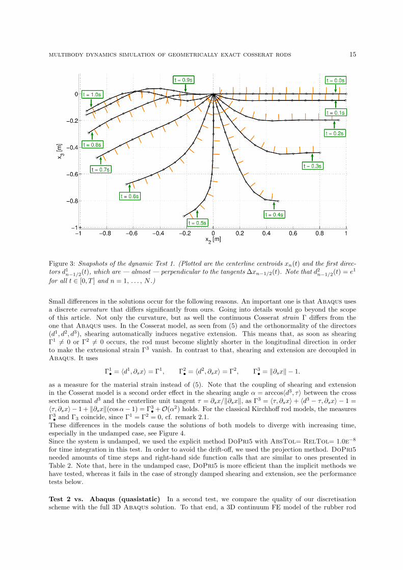
Figure 3: Snapshots of the dynamic Test 1. (Plotted are the centerline centroids xn(t) and the first direc-tors d1

n−1/2(t), which are — almost — perpendicular to the tangents ∆xn−1/2(t). Note that d2n−1/2(t) = e1

for all t ∈ [0, T ] and n = 1, . . . , N .)

Small differences in the solutions occur for the following reasons. An important one is that Abaqus usesa discrete curvature that differs significantly from ours. Going into details would go beyond the scopeof this article. Not only the curvature, but as well the continuous Cosserat strain Γ differs from theone that Abaqus uses. In the Cosserat model, as seen from (5) and the orthonormality of the directors(d1, d2, d3), shearing automatically induces negative extension. This means that, as soon as shearingΓ1 6= 0 or Γ2 6= 0 occurs, the rod must become slightly shorter in the longitudinal direction in orderto make the extensional strain Γ3 vanish. In contrast to that, shearing and extension are decoupled inAbaqus. It uses

Γ1• = 〈d1, ∂sx〉 = Γ1, Γ2

• = 〈d2, ∂sx〉 = Γ2, Γ3• = ‖∂sx‖ − 1.

as a measure for the material strain instead of (5). Note that the coupling of shearing and extensionin the Cosserat model is a second order effect in the shearing angle α = arccos〈d3, τ〉 between the crosssection normal d3 and the centerline unit tangent τ = ∂sx/‖∂sx‖, as Γ3 = 〈τ, ∂sx〉 + 〈d3 − τ, ∂sx〉 − 1 =〈τ, ∂sx〉 − 1 + ‖∂sx‖(cosα− 1) = Γ3

• +O(α2) holds. For the classical Kirchhoff rod models, the measuresΓ3• and Γ3 coincide, since Γ1 = Γ2 = 0, cf. remark 2.1.

These differences in the models cause the solutions of both models to diverge with increasing time,especially in the undamped case, see Figure 4.Since the system is undamped, we used the explicit method DoPri5 with AbsTol= RelTol= 1.0e−8

for time integration in this test. In order to avoid the drift-off, we used the projection method. DoPri5

needed amounts of time steps and right-hand side function calls that are similar to ones presented inTable 2. Note that, here in the undamped case, DoPri5 is more efficient than the implicit methods wehave tested, whereas it fails in the case of strongly damped shearing and extension, see the performancetests below.

Test 2 vs. Abaqus (quasistatic) In a second test, we compare the quality of our discretisationscheme with the full 3D Abaqus solution. To that end, a 3D continuum FE model of the rubber rod


Figure 4: Dynamical comparison with Abaqus 1D finite element solution (Test 1). Plotted are x2(t),x3(t), d1

3(t) = 〈e3, d1(t)〉, M2(t) = EI2K2(t), F 1(t) = GA1Γ

1(t), F 3(t) = EAΓ3(t) according to (16).


of Test 1 has been set up in Abaqus. It is discretised with 160 (in longitudinal direction) × 12 (in thecross section) continuum/brick elements of type C3D8; in total, these are 1920 elements. We considerthe scenario that is plotted in Figure 5. It includes a non-trivial coupling of bending and torsion. Thefully clamped boundary conditions (x0(t), p0(t)) and (xN (t), pN (t)) are chosen in the way that the rodtraverses the shape of the Greek letter ‘γ’ (front view) or the Greek letter ‘Ω’ (side view).To be more precisely, we push the boundary centroids together along the e2-axis,

x0(t) =L

2te2, xN (t) = L

(

1 − t

2

)

e2,

and turn around the boundary quaternions

p0(t) = ℘(

t,1 − e1 − e2 − e3

2,1 − e1 + e2 + e3

2

)

, pN (t) = ℘(

t,1 − e1 − e2 − e3

2,−1 − e1 + e2 + e3

2

)

,

by an angle of π/2. Here the function

℘(t, q0, q1) =1

sin θ

(

sin(

(1 − t)θ)

q0 + sin(tθ)q1

)

, θ = arccos〈q0, q1〉

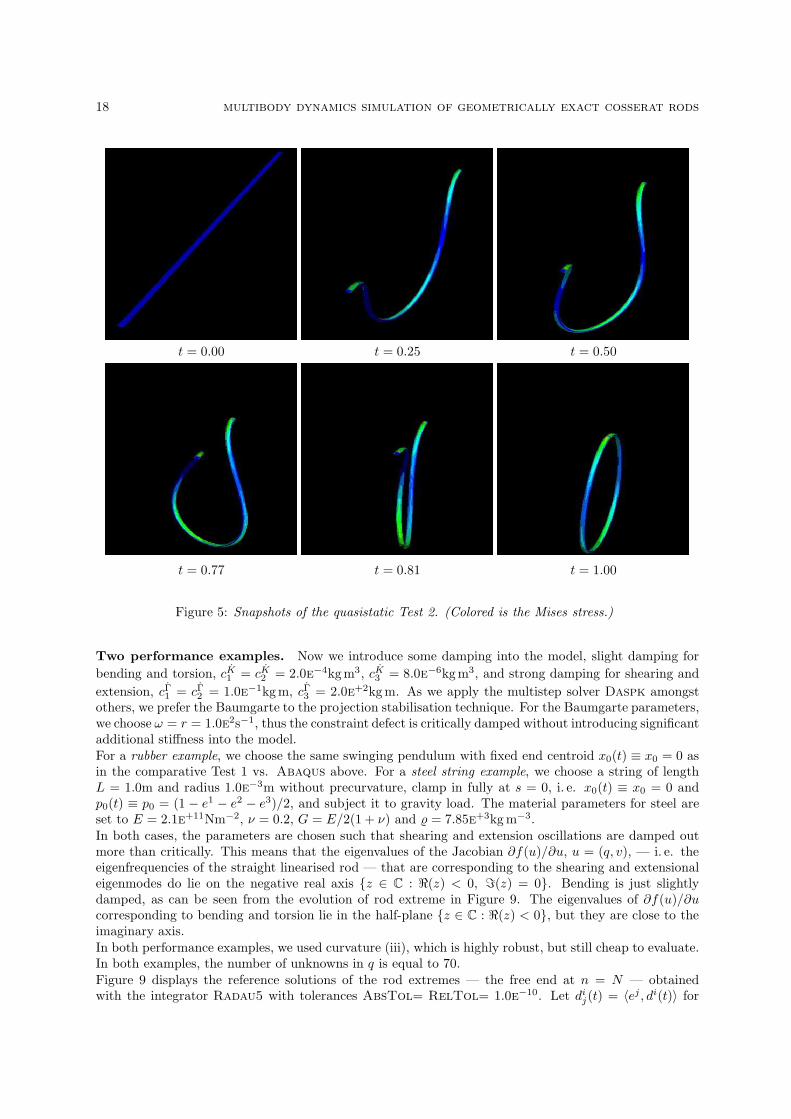
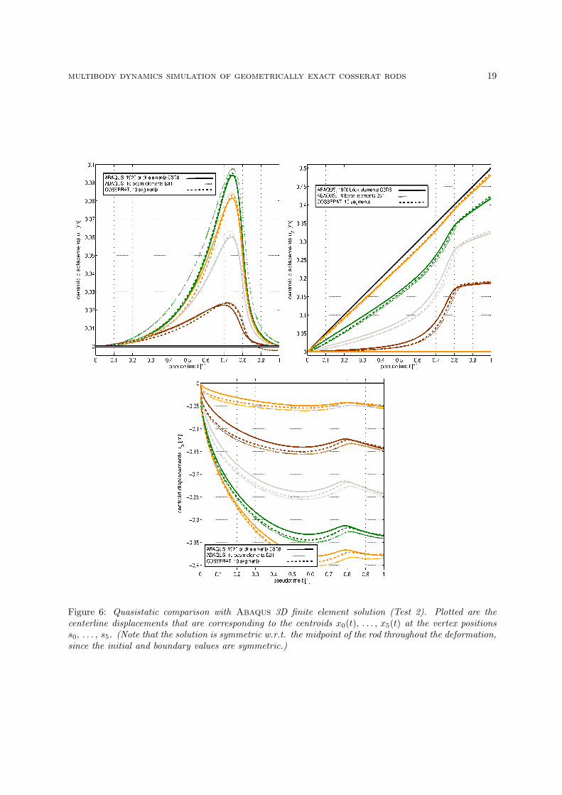
interpolates q0, q1 ∈ S3, such that q0 6= −q1, spherically linearly in the interval t ∈ [0, 1]. In thisexample, t ∈ [0, 1] is a non-dimensional, fictive time, which we prefer to call ‘pseudotime’. Note that theboundary frames R(p0(t)) resp. R(pN(t)) turn around the e2-axis by an angle of π resp. −π and thatR(p0(1)) = R(pN (1)) for t = 1, since p0(1) = −pN(1).Figure 6 shows fine agreement of the results of our discrete Cosserat model. The results are competitiveto the results obtained by Abaqus shear flexible beam elements B31, see Figure 6. We emphasise thatfor our discrete Cosserat rod model, we took only N = 10 segments. Numerical experiments indicatethat the proposed discretisation is a second order approximation of the continuous equations (20) in theequidistant case [38].These results as well confirm that the Cosserat rod theory is an excellent approximation to the fullthree-dimensional theory. Clearly, the thinner the rod, the better the agreement with the 3D solution.Interestingly, the centerline of the 3D solution at t = 1 — after self-intersection — for this scenario liesin the plane x : x1 = 0, see Figure 5. So does ours, in contrast to the Abaqus B31 beam solution. Seethe results for the x1-displacement at t = 1 in Figure 6.

Let us finally give some comments, how we solved the quasistatic problem. The quasistatic balanceequations of forces and moments are obtained from the dynamical ones (21) by letting q = v = 0,q = v = 0, yielding

0 = F(q, t) − G(q)⊤λ0 = g(q)

(31)

with the right hand side forces F(q, t) = F(t) − ∂qV(q, t). We solved this problem, as it is standard innonlinear incremental elastostatics, see e. g. [46] for the unconstrained case. The incremental form of(31) is obtained by time differentiation with respect to the pseudotime t,

(

q

λ

)

=

(

∂2qqV(q, t) + ∂2

qqg[·, λ] G(q)⊤

G(q) 0

)−1 (

∂tF(q, t)0

)

. (32)

This can be interpreted as the index reduced version — the underlying ODE — of the index one (D)AE(31). The inverse of the matrix in (32) constitutes the stiffness-constraint matrix of the system.In our example, 25 equidistant pseudotime steps (= ‘increments’) along [0, 1] were sufficient to solvethe problem. In each step, we applied an explicit Euler step from (32) as a predictor, followed by afull Newton iteration to project the solution back onto the constraint manifold, which is given by (31).Typically about 4 to 6 corrector iterations were sufficient to have the balance of forces and moments (31)satisfied up to roundoff errors. However, we did not focus on a good or an even optimal numerical schemefor quasistatics, including e. g. automatic pseudotime stepsize selection.


t = 0.00 t = 0.25 t = 0.50

t = 0.77 t = 0.81 t = 1.00

Figure 5: Snapshots of the quasistatic Test 2. (Colored is the Mises stress.)

Two performance examples. Now we introduce some damping into the model, slight damping for

bending and torsion, cK1 = cK

2 = 2.0e−4kgm3, cK3 = 8.0e−6kgm3, and strong damping for shearing and

extension, cΓ1 = cΓ

2 = 1.0e−1kgm, cΓ3 = 2.0e+2kgm. As we apply the multistep solver Daspk amongst

others, we prefer the Baumgarte to the projection stabilisation technique. For the Baumgarte parameters,we choose ω = r = 1.0e2s−1, thus the constraint defect is critically damped without introducing significantadditional stiffness into the model.For a rubber example, we choose the same swinging pendulum with fixed end centroid x0(t) ≡ x0 = 0 asin the comparative Test 1 vs. Abaqus above. For a steel string example, we choose a string of lengthL = 1.0m and radius 1.0e−3m without precurvature, clamp in fully at s = 0, i. e. x0(t) ≡ x0 = 0 andp0(t) ≡ p0 = (1 − e1 − e2 − e3)/2, and subject it to gravity load. The material parameters for steel areset to E = 2.1e+11Nm−2, ν = 0.2, G = E/2(1 + ν) and = 7.85e+3kg m−3.In both cases, the parameters are chosen such that shearing and extension oscillations are damped outmore than critically. This means that the eigenvalues of the Jacobian ∂f(u)/∂u, u = (q, v), — i. e. theeigenfrequencies of the straight linearised rod — that are corresponding to the shearing and extensionaleigenmodes do lie on the negative real axis z ∈ C : ℜ(z) < 0, ℑ(z) = 0. Bending is just slightlydamped, as can be seen from the evolution of rod extreme in Figure 9. The eigenvalues of ∂f(u)/∂ucorresponding to bending and torsion lie in the half-plane z ∈ C : ℜ(z) < 0, but they are close to theimaginary axis.In both performance examples, we used curvature (iii), which is highly robust, but still cheap to evaluate.In both examples, the number of unknowns in q is equal to 70.Figure 9 displays the reference solutions of the rod extremes — the free end at n = N — obtainedwith the integrator Radau5 with tolerances AbsTol= RelTol= 1.0e−10. Let di

j(t) = 〈ej , di(t)〉 for


Figure 6: Quasistatic comparison with Abaqus 3D finite element solution (Test 2). Plotted are thecenterline displacements that are corresponding to the centroids x0(t), . . . , x5(t) at the vertex positionss0, . . . , s5. (Note that the solution is symmetric w.r.t. the midpoint of the rod throughout the deformation,since the initial and boundary values are symmetric.)


Figure 7: Computational times and accuracies for different solvers. (The markers correspond to integratortolerances Tol= RelTol= AbsTol= 1.0e−2, . . . , 1.0e−8, cf. as well the corresponding solver statisticsin Tables 2 and 3.)

Figure 8: Step size behaviour for different solvers. (AbsTol= RelTol= 1.0e−3)


Figure 9: The reference solution at the rod extremes at n = N = 10. Here d12(t) = 〈e2, d1(t)〉 denotes the

e2-component of the director d1(t).

Tol Radau5 Seulex Rodas Daspk DoPri5

# f 12 089 2 725 4 050 1 408 331 61010−2 # ∂f/∂u 821 335 600 319 0

# steps 1 645 453 688 478 55 268# f 12 555 8 882 4 764 3 358 331 610

10−3 # ∂f/∂u 877 433 769 458 0# steps 1 714 584 799 1 508 55 268# f 14 679 14 066 7 242 4 403 331 622

10−4 # ∂f/∂u 1 071 463 1 202 427 0# steps 2 050 487 1 208 2 299 55 270# f 21 187 22 311 12 990 6 075 331 694

10−5 # ∂f/∂u 1 507 443 2 165 437 0# steps 2 910 473 2 165 3 263 55 282# f 26 285 38 742 25 440 7 301 332 228

10−6 # ∂f/∂u 1 809 551 4 240 438 0# steps 3 354 628 4 240 3 948 55 371# f 27 463 46 864 54 588 9 659 337 184

10−7 # ∂f/∂u 2 020 654 9 098 443 0# steps 3 224 659 9 098 5 551 56 179# f 33 829 59 751 125 382 12 952 364 376

10−8 # ∂f/∂u 2 584 895 20 897 471 0# steps 3 813 899 20 897 7 703 60 729

Table 2: Solver statistics for rubber rod performance example. (Here T = 10s).


Tol Radau5 Seulex Rodas Daspk DoPri5

# f 30 804 11 450 10 423 6 810 9 211 23210−2 # ∂f/∂u 2 096 1 539 1 568 1 670 0

# steps 4 210 2 667 1 771 1 865 1 535 205# f 31 355 19 073 15 040 6 450 9 211 244

10−3 # ∂f/∂u 2 146 2 136 2 430 1 973 0# steps 4 323 3 062 2 522 1 697 1 535 207# f 35 087 39 904 24 183 10 019 9 211 256

10−4 # ∂f/∂u 2 296 3 669 3 963 2 544 0# steps 5 007 4 190 4 044 3 499 1 535 209# f 44 426 77 994 47 438 30 288 9 211 268

10−5 # ∂f/∂u 2 985 3 374 7 848 9 144 0# steps 6 715 4 428 2 918 11 417 1 535 211# f 74 581 127 326 153 475 81 948 9 211 298

10−6 # ∂f/∂u 4 218 4 247 25 525 33 502 0# steps 12 075 4 342 25 590 26 983 1 535 216# f 107 035 533 384 449 887 69 220 9 211 304

10−7 # ∂f/∂u 6 915 17 868 74 862 20 244 0# steps 15 972 18 010 75 005 31 517 1 535 217# f 129 280 1 720 395 1 146 392 138 874 9 211 310

10−8 # ∂f/∂u 7 853 57 654 190 917 5 961 0# steps 17 272 57 780 191 095 98 652 1 535 218

Table 3: Solver statistics for steel string performance example. (Here T = 10s).

i, j = 1, 2, 3 denote the jth component of the ith director w. r. t. the global system (e1, e2, e3). Since bothexamples are plane scenarios, we have d2(t) ≡ e1, d1

1(t) ≡ d31(t) ≡ 0 and x1(t) ≡ 0 in both cases. Thus,

from the information given in Figure 9 and the orthonormality of the directors, the complete solution —the centroid x(t) and the frame R(t) = (d1(t), d2(t), d3(t)) — can be easily reconstructed.

Figure 7 shows the computational times for the solvers Radau5 (an implicit Runge-Kutta method),Seulex (an extrapolation method), Rodas (a Rosenbrock method), DoPri5 (an explicit Runge-Kuttamethod) from [27, 28, 29, 43] and Daspk (= Dassl, a multistep BDF method) from [49] at severaltolerances. For all the computations we choose Tol= AbsTol= RelTol, discarding the error controlfor the Lagrange multipliers. Clearly, the problem is stiff even for rubber material because of the presenceof the high extensional and shearing frequencies [38]. Thus, DoPri5 fails, the corresponding step sizesin Figure 8 indicate that it runs at the stability limit. In contrast to that, the four stiff solvers revealsatisfactory step size behaviour. We remark that Figure 8 displays just an excerpt of the time stephistories for the five solvers. Clearly, the mean time step sizes of the implicit integrators increase slightlyalong [0, T ], since the internal total energy is dissipated slightly with time. For Radau5, we did notdiscover any significant difference between the classical and the Gustafsson step size strategy.

For the solvers Radau5, Seulex and Rodas, we chose sparse linear algebra, adapted to second orderODEs, with upper resp. lower bandwidths mujac resp. mljac of the Jacobians ∂f/∂q and ∂f/∂v equalto ten. Radau5 spent about 38% of the total computational time in order to evaluate f and ∂f/∂u,Seulex about 43% and Rodas about 61%. The remaining percentage is needed for (non)linear algebra.Roughly, an evaluation of f needs about 1.06e−5s, which is comparable to [63], but with a much morerobust curvature model, an evaluation of ∂f/∂u needs about 1.02e−4s, this is about ten times larger.

Clearly, for coarse discretisations and rough error control during time integration, Rodas performs best.Here, for the rubber pendulum example, the factor to the real physical time is 47, for the steel stringexample 17. The results that are obtained for coarse tolerances AbsTol= RelTol= 1.0e−2 are stillaccurate enough for virtual reality applications such as industrial path planning, the modeling of cablesand hoses. For more stringent tolerances and high accuracy demands, Radau5 performs best, since it isa high order method.


The computations have been performed on a 2.19 GHz Dual Core AMD (Opteron) machine on one CPUand on one core. For further discussions of special numerical topics in time integration for classicalCosserat and Kirchhoff rods, we refer to [38].

5 Conclusions

We presented a numerically stable and efficient method for the dynamical analysis of Cosserat rods thatcomputes within milliseconds numerical results with an accuracy similar to detailed finite element solu-tions. At its heart, this novel approach is based on a coarse grid finite difference approximation that fol-lows from a discrete variational principle taking into account the overall requirement of frame-indifferenceand considering the material damping by Rayleigh damping terms. A consistent semi-discretisation ofthe continuous dynamical Cosserat partial differential equations of motion is achieved combining twostaggered space grids. From the algorithmic viewpoint, the parametrisation of rotations by quaternionsproved to be very useful. For time integration, standard ODE and DAE solvers were applied.All basic components of this approach are not restricted to Cosserat rods and may be extended to plateand shell structures. Further gains in efficiency may be expected from the use of null-space methodsin time integration that are tailored to quaternion representations of the rotational degrees of freedom.The incorporation of geometrical constraints like obstacles in the model is especially interesting from theviewpoint of practical application but yields fundamentally new problems in theory, in space discretisationand in the final full (space-time) integration of the equations of motion. A reference implementation ofthe proposed approach in a virtual reality tool for vehicle design is under development.

A Objective finite difference approximations of curvature

The numerical evaluation of the potential energy (24) as well as the symbolic computation of its variousgradient terms appearing on the r.h.s. of the discrete balance equations (29) requires explicit algebraicexpressions of the discrete curvatures as generally defined by the finite difference ansatz (25) in terms of theadjacent midpoint quaternions pn±1/2. In the following we present several possible choices of the vertexquaternion pn and the corresponding expression δpn which explicitly lead to the FD approximations (26)of the discrete vertex curvature via the finite difference ansatz (25), including a geometrical interpretationof these expressions via trigonometry and spherical geometry. Recall that δsn = sn+1/2 − sn−1/2 in thesequel. Each ansatz is illustrated in Figure 10.

(i) The simplest variant (see e. g. [63]) is obtained by using the secant δpn = pn+1/2 − pn−1/2 andlinear midpoint interpolation pn = (pn−1/2 + pn+1/2)/2, regardless of the fact that this choice of pn

violates the condition of unit length, and results in ζ(θ) = 1. This choice leads to a ‘soft’ behaviourof the curvature with an increasing size of the relative rotation angle between frames, which resultsin poor stability properties for large bending or torsion angles, as we shall see. Phenomena such as‘quaternion flipping’ (= sign change) might be the consequence.

(ii) Here we choose pn = (pn−1/2 + pn+1/2)/(2 + 2〈pn−1/2, pn+1/2〉)1/2, which is the midpoint of thegreat circle that is joining pn−1/2 to pn+1/2, and the secant δpn = pn+1/2 − pn−1/2. Note that pn

is in S3, if pn−1/2 and pn+1/2 are so. Using the identity ‖p + q‖2 = 2 + 2〈p, q〉 for p, q ∈ S3, this

choice leads to ζ(θ) =√

2/(1 + cos θ).

(iii) The third variant, which is identical to the one discussed in [33] and generalises the definitionsof the discrete vertex bending curvature proposed in [8, 12] for inextensible Kirchhoff rods, maybe obtained by choosing either pn = pn−1/2 combined with a tangential forward difference δpn =pn+1/2/ cos θn − pn−1/2, or pn = pn+1/2 combined with a tangential backward difference δpn =pn+1/2−pn−1/2/ cos θn — or the arithmetic mean of both. Straightforward algebra shows that eachof these choices leads to Knδsn = 2ℑ(Wn)/ℜ(Wn), which corresponds to ζ(θ) = 1/ cos(θ). Inter-esting properties of this curvature approximation are its ‘flip invariance’ as well as the singularity— yielding infinite bending and torsional stiffness — at θn → π/2, which prevents the occurrenceof degenerate configurations at finite deformation energy. (See also [33] for a discussion.)


Figure 10: Geometric illustration of the interpolation and finite difference ansatzes used in the discreteapproximations of the vertex curvature Kn

(iv) To obtain the fourth variant, we use pn as in (ii), combined with the tangential central differenceδpn = (pn+1/2 −pn−1/2)/ cos(θn/2). Similarly to (iii), curvature (iv) displays a stiffening behaviourat increasing angles, with a singularity (corresponding to infinite stiffness) occurring at θn → π,i. e. at an angle twice as large as for (iii).

(v) We obtain this last variant on the basis of a geodesic interpolation connecting the pair of unitquaternions pn−1/2 and pn+1/2, assumed to be non-antipodal (i. e. pn+1/2 6= −pn−1/2), on the greatcircle arc parametrised by the spherically linear interpolating function [59]

℘(s) =1

sin θn

(

sin(

(1 − σ)θn

)

pn−1/2 + sin(

σθn

)

pn+1/2

)∣

∣

∣

σ=(s−sn−1/2)/δsn

. (33)

An evaluation of the product ℘(s)∂s℘(s) at any curve parameter s ∈ [sn−1/2, sn+1/2] reveals thewell known fact that ℘(s)∂s℘(s) is completely independent of s and depends solely on the endpointspn−1/2 and pn+1/2, see [20, 59]. This variant, resulting in the expression ζ(θ) in (v), is thus applicablewithout modification in the case of a non-equidistant discretisation as well. Recently this variantwas applied as special case within the so-called ‘geodesic finite element’ approach proposed by [53],where it appears naturally due to the fact that the great circle arcs (33) are the geodesic lines inthe manifold / sphere S3 [59].

Let us translate the five proposed discrete curvature measures from the quaternionic into the settingof rotations in Euclidean space. To that end, we rewrite the material quotient/difference quaternionWn in the form Wn = cos(φn/2) + sin(φn/2)un with a purely imaginary (= vector) unit quaternionun ∈ S3 ∩ ℑ(H), which represents the material unit axis of rotation, and the Euclidean difference angle


φn, which is precisely twice the quaternionic difference angle θn [23, 25], i. e. φn = 2θn. Then, it isstraightforward to see that the five proposed curvature measures correspond to

(i) Kn =2

δsnsin

(φn

2

)

un, (ii) Kn =4

δsnsin

(φn

4

)

un, (iii) Kn =2

δsntan

(φn

2

)

un,

(iv) Kn =4

δsntan

(φn

4

)

un, (v) Kn =φn

δsnun

in the Euclidean representation. It is worth mentioning that the families of Euclidean characteristicgenerating functions

η(φ) = m sin( φ

m

)

, η(φ) = m tan( φ

m

)

, η(φ) = φ (34)

with any integer – or even real – parameter m ≥ 1 all satisfy the conditions η(0) = 0 and η′(0) = 1, whichare essential for the consistency of our finite difference schemes for small bending and torsion angles φn.The functions η(φ) all are strictly increasing on the interval [0, φ∗), where

(i) φ∗ = π, (ii) φ∗ = 2π, (iii) φ∗ = π, (iv) φ∗ = 2π, (v) φ∗ = ∞.

The tangent generators η(φ) of curvatures (iii) and (iv) even become singular at φ∗, i. e. η(φ) → ∞ forφ → φ∗. Note that these singularities, yielding infinite bending and torsional stiffnesses at φ∗, are notthe result of a hyperelastic constitutive material law — we use a linear one — but are caused by differentgeometric approaches in the spatial discretisation. Figure 11 displays the sine and tangent generators(34) for the cases m = 2, 4,∞ corresponding to our discrete curvatures (i) to (v).Curvature (v) can be considered as the limit case of both the sine and tangent generator family for m →∞. Concerning its quaternionic characteristic ζ(θ) = θ/ sin θ, one should remark that the compositionw 7→ (ζ arccos)(w) = arccos(w)/

√1 − w2 is clearly analytical and especially admits Taylor expansion

in a neighbourhood of w = 1, which corresponds to pn−1/2 = pn+1/2.The suggested curvature measures all differ in algebraic complexity (see Table 1) and numerical robustness(e. g. desired singularities for φ → φ⋆). However, from the analytical viewpoint, it is not yet clear, whichof them is ‘the best’. Asymptotically for |φ| ≪ 1, they all coincide, see Figure 11.

References

[1] Antman S. S.: Kirchhoff’s problem for nonlinearly elastic rods. Quarterly of applied mathematics, 32, 221–240, 1974.

[2] Antman S. S.: Dynamical problems for geometrically exact theories of nonlinearly viscoelastic rods. Journal ofnonlinear science, 6, 1–18, 1996.

[3] Antman S. S.: Nonlinear problems of elasticity. Springer, 2005.

[4] Arnold M.: Numerical methods for simulation in applied mechanics. In: Simulation techniques for applied mechanics(Eds: Arnold M., Schiehlen W.), Springer, 191–246, 2008.

[5] Bauchau O.A., Epple A., Bottasso C. L.: Scaling of constraints and augmented Lagrangian formulations inmultibody dynamics simulations. Journal of computational and nonlinear dynamics, 4 (2), 2009.

[6] Bauchau O.A., Trainelli L.: The vectorial parametrization of rotation. Nonlinear dynamics, 32 (1), 71–92, 2003.

[7] Bauchau O.A., Epple A., Heo S.: Interpolation of finite rotations in flexible multi–body dynamics simulations.Proceedings of the institution of mechanical engineers, 222 (4) Part K: Multi-body dynamics, 353–366, 2008.

[8] Bergou M., Wardetzky M., Robinson S., Audoly B., Grinspun E.: Discrete elastic rods. ACM transactionon graphics, 27 (3), 63:1–63:12, 2008.

[9] Betsch P., Siebert R.: Rigid body dynamics in terms of quaternions: Hamiltonian formulation and conservingnumerical integration. International journal for numerical methods in engineering, 79 (4), 444–473, 2009.

[10] Betsch P., Steinmann P.: A DAE approach to flexible multibody dynamics. Multibody system dynamics, 8, 365–389, 2002.


Figure 11: Euclidean characteristic generating functions η(φ) of curvature corresponding to the sin– andtan–family of vectorial rotation parametrisations [6] in the cases m = 2, 4,∞.

[11] Betsch P., Steinmann P.: Frame-indifferent beam finite elements based upon the geometrically exact beam theory.International journal for numerical methods in engineering, 54, 1755–1788, 2002.

[12] Bobenko A. I., Suris Y. B.: Discrete time Lagrangian mechanics on Lie groups with an application to the Lagrangetop. Communications in mathematical physics, 204, 147–188, 1999.

[13] Cardona A., Geradin M.: A beam finite element nonlinear theory with finite rotations. International journal fornumerical methods in engineering, 26, 2403–2434, 1998.

[14] Cardona A., Geradin M.: Flexible multibody dynamics. A finite element approach. Wiley, 2001.

[15] Cartan H.: Differential Forms, Kershaw Publishing, 1971, reprinted by Dover, 2006.

[16] Chouaieb N., Maddocks J.H.: Kirchhoff’s problem of helical equilibria of uniform rods, Journal of elasticity, 77,221–247, 2004.

[17] Cowper G.R.: The shear coefficient in Timoshenko’s beam theory. Journal of applied mechanics, 68 (1), 87–92,1968.

[18] Craig R.R. jr., Kurdila A. J.: Fundamentals of Structural Dynamics. Wiley, 2006.

[19] Craig R.R. jr., Bampton M.C.C.: Coupling of substructures for dynamic analysis. AIAA journal, 6 (7), 1968.

[20] Crisfield M.A., Jelenic G.: Objectivity of strain measures in the geometrically exact three-dimensional beamtheory and its finite element implementation. Proceedings of the Royal Society London, 455, 1125–1147, 1999.

[21] Dichmann D. J., Maddocks J.H.: An impetus-striction simulation of the dynamics of an elastica. Journal ofnonlinear science, 6, 271–292, 1996.

[22] Dill E.H.: Kirchhoff’s Theory of Rods, Archives for history of exact sciences, 44 (1), 1–23, 1992.

[23] Ebbinghaus H. D. et al.: Numbers. Springer, 1992.

[24] Eich-Soellner E., Fuhrer C.: Numerical methods in multibody dynamics. Teubner, 1998.


[25] Hanson A. J.: Visualizing quaternions. Elsevier, 2005.

[26] Hodges D. H.: Nonlinear composite beam theory. Progress in astronautics and aeronautics, 213, 2006.

[27] Hairer E., Lubich C., Roche M.: The numerical solutions of differential-algebraic systems by Runge-Kuttamethods. Springer lecture notes in mathematics, 1409, 1989.

[28] Hairer E., Noersett S. P., Wanner G.: Solving ordinary differential equations I. Springer, 1993.

[29] Hairer E., Wanner G.: Solving ordinary differential equations II. Springer, 1996.

[30] Hairer E., Lubich C., Wanner G.: Geometric numerical integration. Springer, 2002.

[31] Ibrahimbegovic A.: On finite element implementations of geometrically nonlinear Reissner’s beam theory: Threedimensional curved beam elements. Computer methods in applied mechanics and engineering, 112, 11–26, 1995.

[32] Ibrahimbegovic A., Frey F.: Finite element analysis of linear and nonlinear planar deformations of elastic initiallycurved beams. International journal for numerical methods in engineering, 36, 3239–3258, 1992.

[33] Jung P., Leyendecker S., Linn J., Ortiz M.: A discrete mechanics approach to Cosserat rod theory — PartI: Static equilibria, International journal for numerical methods in engineering, in press, DOI: 10.1002/nme.2950.Preprint: Berichte des ITWM Nr. 183, 2010.

[34] Kuipers J. B.: Quaternions and rotation sequences. Princeton university press, 1999.

[35] Kehrbaum S., Maddocks J.H.: Elastic rods, rigid bodies, quaternions and the last quadrature. Philosophicaltransactions of the royal society London A, 355, 2117–2136, 1997.

[36] Kirchhoff G.: Uber das Gleichgewicht und die Bewegung eines unendlich dunnen elastischen Stabes, Journal fur diereine und angewandte Mathematik (Crelle), 56, 285–343, 1859.

[37] Langer J., Singer D.A.: Lagrangian aspects of the Kirchhoff elastic rod, SIAM Review, 38 (4), 605–618, 1996.

[38] Lang H., Arnold M.: Numerical aspects in the dynamic simulation of geometrically exact rods. Accepted forpublication in Applied numerical mathematics. Preprint: Berichte des ITWM Kaiserslautern, 179, 2009.

[39] Lang H., Linn J.: Lagrangian field theory in space-time for geometrically exact Cosserat rods. Preprint: Berichtedes ITWM Kaiserslautern, 150, 2009.

[40] Linn J., Stephan T., Carlsson J., Bohlin R.: Fast simulation of quasistatic cable deformations for Virtual Realityapplications, in: L.L. Bonilla et al. (Eds.): Progress in Industrial Mathematics at ECMI 2006, 247–253, Springer,2007. Preprint: Berichte des ITWM Kaiserslautern, 143.

[41] Linn J., Stephan T.: Simulation of quasistatic deformations using discrete rod models. MULTIBODY DYNAMICS2007, ECCOMAS Thematic Conference. Eds: C. L. Bottasso, P. Masarati, L. Trainelli, Milano, Italy, 25-28 June2007. Preprint: Berichte des ITWM Kaiserslautern, 144.

[42] Love A.E. H.: A Treatise on the Mathematical Theory of Elasticity (4th edition). Cambridge University Press, 1927,reprinted by Dover, 1944.

[43] Lubich C.: Integration of stiff mechanical systems by Runge-Kutta methods. Journal of applied mathematics andphysics, 44, 1022–1053, 1993.

[44] Maddocks J.H.: Stability of nonlinearly elastic rods, Archive for rational mechanics and analysis, 85, 311–354,1984.

[45] Marheineke N., Wegener R.: Fiber Dynamics in Turbulent Flows: General Modeling Framework SIAM journalon applied mathematics, 66 (5), 1703–1726, 2006.

[46] Matthies H., Strang G.: The solution of nonlinear finite element equations. International journal for numericalmethods in engineering, 14, 1613–1626, 1967.

[47] Richtmyer R.D., Morton K.W.: Difference methods for initial value problems. Interscience publishers, New York,1967.

[48] Nizette M., Goriely A.: Towards a classification of Euler–Kirchhoff filaments, Journal of mathematical physics,40 (6), 2830–2866, 1999.

[49] Petzold L.R.: A description of DASSL: A differential algebraic system solver. In: Scientific computing, SteplemanR. S. (Ed.), North-Holland, Amsterdam, 1981.

[50] Rabier P. J., Rheinboldt W.C.: Non-holonomic motion of rigid mechanical systems from a DAE viewpoint. SIAM,2000.


[51] Reissner E.: On one-dimensional large-displacement finite-strain beam theory, Studies in applied mathematics, 52,87–95, 1973.

[52] Romero I.: The interpolation of rotations and its application to finite-element models of geometrically exact rods.Computational mechanics, 34, 121–133, 2004.

[53] Sander O.: Geodesic finite elements for Cosserat rods. International journal for numerical methods in engineering,82 (13), 1645–1670, 2009.

[54] Schiehlen W.O.: Multibody system dynamics: Roots and perspectives. Multibody system dynamics, 1, 149–188,1997.

[55] Schiehlen W., Eberhard P.: Technische Dynamik. Modelle fur Regelung und Simulation. Teubner, 2004.

[56] Schwab A. L., Meijaard P. J.: How to draw Euler angles and utilize Euler parameters. Proceedings of IDETC/CIE,2008.

[57] Shabana A. A.: Flexible multibody dynamics: Review of past and recent developments. Multibody system dynamics,1, 189–222, 1997.

[58] Shabana A. A.: Dynamics of multibody systems. Cambridge, 2005.

[59] Shoemake K.: Animating rotation with quaternion curves. ACM SIGGRAPH Computer Graphics, 19 (3), 245–254,1985.

[60] Simeon B.: Numerical analysis of flexible multibody dynamics. Multibody system dynamics, 6, 305–325, 2001.

[61] Simo J.C.: A finite strain beam formulation. The three dimensional dynamic problem. Part I. Computer methodsin applied mechanics and engineering, 49, 55–70, 1985.

[62] Simo J.C., Vu-Quoc L.: A three dimensional finite strain rod model. Part II. Computer methods in appliedmechanics and engineering, 58, 79–116, 1986.

[63] Spillmann J., Teschner M.: CoRdE. Cosserat rod elements for the dynamic simulation of one-dimensional elasticobjects. Eurographics/ACM SIGGRAPH, 1–10, 2007.

[64] Zupan E., Maje M., Zupan D.: The quaternion–based three–dimensional beam theory. Computer methods inapplied mechanics and engineering, 198, 3944–3956, 2009.

Multibody dynamics simulation of geometrically exact … · 2012-08-13 · multibody dynamics...

Documents

Transcript of Multibody dynamics simulation of geometrically exact … · 2012-08-13 · multibody dynamics...