Multi-Period Planning, Design and Strategic Models for...
62
1 Multi-Period Planning, Design and Strategic Models for Long-Term, Quality-Sensitive Shale Gas Development Markus G. Drouven & Ignacio E. Grossmann Department of Chemical Engineering Carnegie Mellon University Pittsburgh, PA, 15213, USA In this work we address the long-term, quality-sensitive shale gas development problem. This problem involves planning, design and strategic decisions such as where, when and how many shale gas wells to drill, where to lay out gathering pipelines, as well as which delivery agreements to arrange. Our objective is to use computational models to identify the most profitable shale gas development strategies. For this purpose we propose a large-scale, nonconvex, mixed-integer nonlinear programming (MINLP) model. We rely on generalized disjunctive programming (GDP) to systematically derive the building blocks of this model. Based on a tailor-designed solution strategy we identify near-global solutions to the resulting large-scale problems. Finally, we apply the proposed modeling framework to two case studies based on real data to quantify the value of optimization models for shale gas development. Our results suggest that the proposed models can increase upstream operators’ profitability by several millions of dollars. Introduction It is expected that by 2040 shale gas will eventually account for at least 50% of total natural gas production in the United States 1 . This is a remarkable development considering the fact that as of 2005 the United States were producing hardly any natural gas from shale formations. However, given the projected production increase virtually all stages of the existing natural gas supply chain will need new, expanded, and/or upgraded infrastructure: gas gathering pipelines, processing facilities, transmission pipelines, storage facilities and many more 2 . The objective of this work is to develop high-level, computational decision-making support tools that allow upstream operators to identify optimal shale gas development strategies. Shale gas extraction involves a combination of vertical drilling, horizontal drilling and hydraulic fracturing. Hydraulic fracturing refers to the injection of a fracturing fluid into a geologically tight formation under high pressure of up to 70 MPa. This well stimulation creates fractures in the sub-surface ________________________________ Correspondence concerning this article should be addressed to I. E. Grossmann at [email protected]
Transcript of Multi-Period Planning, Design and Strategic Models for...
1
Multi-Period Planning, Design and Strategic Models for
Long-Term, Quality-Sensitive Shale Gas Development
Markus G. Drouven & Ignacio E. Grossmann
Department of Chemical Engineering
Carnegie Mellon University
Pittsburgh, PA, 15213, USA
In this work we address the long-term, quality-sensitive shale gas development problem. This problem
involves planning, design and strategic decisions such as where, when and how many shale gas wells to
drill, where to lay out gathering pipelines, as well as which delivery agreements to arrange. Our objective
is to use computational models to identify the most profitable shale gas development strategies. For this
purpose we propose a large-scale, nonconvex, mixed-integer nonlinear programming (MINLP) model.
We rely on generalized disjunctive programming (GDP) to systematically derive the building blocks of
this model. Based on a tailor-designed solution strategy we identify near-global solutions to the resulting
large-scale problems. Finally, we apply the proposed modeling framework to two case studies based on
real data to quantify the value of optimization models for shale gas development. Our results suggest that
the proposed models can increase upstream operators’ profitability by several millions of dollars.
Introduction
It is expected that by 2040 shale gas will eventually account for at least 50% of total natural gas production
in the United States1. This is a remarkable development considering the fact that as of 2005 the United
States were producing hardly any natural gas from shale formations. However, given the projected
production increase virtually all stages of the existing natural gas supply chain will need new, expanded,
and/or upgraded infrastructure: gas gathering pipelines, processing facilities, transmission pipelines,
storage facilities and many more2. The objective of this work is to develop high-level, computational
decision-making support tools that allow upstream operators to identify optimal shale gas development
strategies.
Shale gas extraction involves a combination of vertical drilling, horizontal drilling and hydraulic
fracturing. Hydraulic fracturing refers to the injection of a fracturing fluid into a geologically tight
formation under high pressure of up to 70 MPa. This well stimulation creates fractures in the sub-surface
________________________________
Correspondence concerning this article should be addressed to I. E. Grossmann at [email protected]
2
reservoir that locally increase the permeability of the formation which allows trapped gas to flow into the
wellbore and up to the surface. Hydraulic fracturing requires large amounts of water, oftentimes more than
20 million liters of water per well. In addition, operators add proppant and special additives into the water
to keep fractures open and enhance the gas flow into the wellbore. The typical composition of the
fracturing fluid is 90% water, 9% proppant and 1% chemical additives.
Nowadays, upstream operators have the ability to drill as many as 40 horizontal wells from a single well
pad. Fig. 1 illustrates a well pad with merely eight wells. These multi-well pads allow the operators to
recover large quantities of gas from a single location while reducing the surface disruption to a minimum.
By developing several wells in parallel, operators can also take advantage of economies of scale that lower
the unit cost for drilling a well substantially.
A single well pad is typically developed as follows: Initially, operators construct a temporary well site.
For this purpose the pad is levelled, water impoundments and pits are excavated and an access ramp is
built to the site itself. As soon as the pad construction is concluded, a drilling rig is moved on site and
assembled. Drilling may take several months depending on how many wells are drilled, how deep they
reach vertically and how far they extend horizontally. Next, completion operations begin. These
operations involve the actual fracturing of the formation that can last for up to two annual quarters
depending on the completion technique. Commonly, the lateral sections of the wells are stimulated in
stages which are sealed off temporarily and treated individually. During this development phase the
operators need to have large quantities of water stored on site. Once completed, the wells are connected
to the local gathering system and ready for production. Today it is expected that shale wells will produce
gas for up to 10-25 years.
Shale gas wells are characterized by very high initial production rates of up to 280,000 m3/day that are
followed by drastic declines as high as 65-85% within the first year. A typical shale well may in fact
produce more than half of its total estimated ultimate recovery (EUR) within the first year of production.
The initial peak in production is due to the sudden release of trapped gas after the well stimulation.
Eventually though, the production decline is driven by pressure depletion and the inherently low
permeability of the reservoir. The characteristic shale well production profiles as seen in Fig. 2 present
major challenges to the operators who often enter into long-term take-away agreements with pipeline
companies, and commit to delivering an agreed amount of gas over time. Given the inherent declines in
production rates, it can be difficult to meet these constraints at times, and hence operators are forced to
turn new wells in line continuously to honor these terms.
3
Shale gas wells produce different qualities of natural gas. Operators traditionally distinguish between dry
gas and wet gas. The primary component of both gas qualities is methane. The key difference between
them is that dry gas contains very few so-called natural gas liquids (NGLs). These NGLs are light
hydrocarbons that include ethane, propane, pentane, butane and natural gasoline. In wet gas, on the other
hand, these components can account for up to 15% of the total gas. In addition, the extracted gas may also
contain impurities such as nitrogen, carbon dioxide or hydrogen sulfide. For the operators the distinction
between different gas qualities is important for a number of reasons.
For one, gas that is delivered to interstate transmission pipelines must be within a specific heating value
range (approximately 900 kJ/mol), and it may contain no more than trace components of hydrogen sulfide
or carbon dioxide, for example. A gas stream that meets these specifications is considered pipeline-quality
gas3. In order to meet these specifications the produced raw gas generally needs to be treated, i.e., purified
at dedicated processing plants. The primary purpose of these processing plants is to extract natural gas
liquids and undesirable components from the raw gas stream and return pipeline-quality gas to the
operators. This processing service is typically not performed by the operators themselves, but rather
provided by midstream processors as an independent, contract based businesses.
Generally, dry gas – which contains mostly methane (heating value: 889 kJ/mol) – can be marketed as
pipeline-quality gas and operators do not have to pay for processing. The NGL components contained in
wet gas, however, increase the heating value of the gas mixture significantly above pipeline specifications
(ethane: 1,560 kJ/mol, propane: 2,220 kJ/mol, pentane: 3,507 kJ/mol). Therefore, wet gas always has to
be purified prior to its delivery – which results in non-negligible processing expenses to the upstream
operator. The intriguing tradeoff, though, is that the NGLs contained in wet gas oftentimes trade at a
premium to pipeline-quality gas, i.e., their sales prices are significantly higher. Hence, the distinction
between dry gas and wet gas is very important in terms of the shale gas development problem.
The quality issue of shale gas development is further complicated by the fact that the composition of the
extracted gas may vary spatially within a particular gathering system. Therefore, it is oftentimes
problematic to classify a development area as distinctively wet or dry. Since individual wells will be
feeding different gas qualities into one and the same gathering system at varying production rates, it may
be non-obvious for the decision-makers to determine: a) which wells to develop over time with respect to
a given gas and liquids price forecast, b) when and how to blend gas streams to meet quality specifications,
or c) when and how much processing capacity to procure from a midstream processor. Hence, we postulate
in this work that the shale gas development problem is truly quality-sensitive, i.e., the quality of the
extracted gas determines decisively which development strategies are profitable for the operator, and
which ones may not be feasible.

4
The paper is organized as follows. After presenting a brief literature review on related publications, we
summarize the scope of our work in terms of a general problem statement and list the modeling
assumptions. In the following section we present the proposed models for the long-term shale gas
development problem: one addresses the development project with only one delivery node, and the other
model captures the general, multiple delivery node development problem. While the former can be solved
to global optimality with an MILP model, the general formulation yields a nonconvex MINLP for which
we describe a solution strategy that is designed to identify near-global and optimal solutions. Finally, we
apply the models to two case studies that demonstrate and quantify the value of computational models for
long-term shale gas development.
Literature Review
To date, the long-term shale gas development problem has received little attention in literature. Previous
work has been focused primarily on conventional on- and offshore oil and gas field development planning,
and the body of literature on this topic is extensive. For instance, Iyer and Grossmann4 propose a discrete-
time, multi-period mixed-integer linear programming (MILP) model for the design and planning of
offshore oilfield infrastructure. The design decisions consider the well drilling schedule, the installation
of well and production platforms, and fluid production rates in every time period to maximize the net
present value. Van den Heever and Grossmann5 address the same problem as Iyer and Grossmann, but
include the nonlinear reservoir performance in the formulation, rendering the model a mixed-integer
nonlinear programming (MINLP). Van den Heever et al.6 extend the oil field development problem by
considering complex economic objectives, such as fiscal rules and royalty payments. Goel and
Grossmann7 consider the offshore gas field development planning problem under uncertainty in reservoir
reserves, for which they propose a stochastic programming approach. Selot et al.8 specifically address
natural gas production systems with multiple gas qualities. The authors develop a single-period model for
a limited planning horizon of one week and consider gas quality specifications at delivery nodes. Tavallali
et al.9 integrate critical elements of upstream oil production and spatiotemporal subsurface dynamics in a
multi-period mathematical programming approach. Knudsen and Foss10 consider late-life shale gas wells
producing at low erratic rates due to reservoir depletion and liquid loading. The authors present a shale
gas well reservoir proxy model and a production scheduling model formulated as a generalized disjunctive
program (GDP) that allow for enhanced gas production through cyclic shut-in based production strategies.
In order to address field-wide multi-pad shale gas systems Knudsen et al.11 propose a Lagrangean
relaxation based decomposition scheme to deal with the dimensionality of the resulting large-scale MILPs.
Furthermore, Knudsen et al.12 make use of the proposed well scheduling models to argue that shale gas
wells could be used for natural gas supply in electric power plants. Yang et al.13 focus on optimization
5
models for shale gas water management. Given an uncertain water availability the authors propose a two-
stage stochastic MILP model based on the State-Task Network (STN) representation to minimize the
expected water related expenses for transportation, treatment, storage and disposal, while accounting for
natural gas sales revenues. Also, Yang et al.14 extended their modeling framework to optimize longer-
term investment decisions using a deterministic MILP model for determining the location and capacity of
water impoundments, piping options, treatment technologies and facility locations, as well as the optimal
fracturing schedule. To the best of our knowledge, Cafaro and Grossmann15 are the first to have addressed
the long-term shale gas development problem from a strategic perspective. The authors propose a large-
scale, nonconvex MINLP model to identify the optimal shale gas supply chain. In the proposed model,
nonlinearities arise from concave power law expressions to represent economies of scale. A major
restriction is that the shale gas composition is assumed to be independent of well pad locations. Recently,
Gao and You16 examine the well-to-wire life cycle of electricity generated from shale gas. In this context,
the authors present a multi-objective, nonconvex MINLP model to optimize the design and operation of
shale gas supply chain networks considering economic and environmental factors.
The models proposed in this work are important extensions of the previous work by Cafaro and
Grossmann15. The following paragraphs summarize the major new developments.
1) We present a novel superstructure for the shale gas development problem that is motivated by real-
world gathering systems. This superstructure captures the distinctive “tree”-structure of typical gas
gathering systems. These systems are characterized by trunk lines that “branch” out into the
development area and eventually “ramify” to the well pads through a tight grid of flow pipelines. In
addition, the superstructure explicitly distinguishes between different delivery options in real-world
shale gas development areas, namely processing sales routes and direct delivery sales arcs.
2) As part of the shale gas development problem upstream operators need to size gathering pipelines and
transmission compressors. Oftentimes the corresponding design variables are treated as continuous
decision variables to simplify the synthesis problem. In this work we consider discrete sizes of pipeline
diameters and compressors, which allows us to use mixed-integer linear constraints for equipment
sizing purposes. More importantly, by restricting the design variables to discrete values, we can
capture economies of scale without dealing with continuous concave cost functions.
3) In this work we also extend the scope of the shale gas development problem to explicitly consider
strategic development decisions, which to the best of our knowledge have not been addressed before.
The aforementioned strategic decisions include: a) the selection of delivery nodes, b) the arrangement
of delivery agreements, and c) the procurement of delivery capacity. These downstream decisions have
6
a major impact on the upstream development of a particular shale gas gathering system and add to the
complexity of the overall development problem.
4) Lastly, we specifically address the general shale gas development problem with multiple delivery
nodes while explicitly considering spatial gas composition variations. These composition variations
are common in real-world gas gathering systems and complicate shale gas development in practice.
On the one hand, upstream operators target different gas qualities depending on prevailing price
forecasts. On the other hand, the operators need to ensure that their gas deliveries satisfy gas quality
specifications at the delivery nodes. The consideration of spatial gas quality variations within multiple
delivery node gathering systems yields a nonconvex MINLP for which we propose a tailor-designed
solution strategy.
General Problem Statement
The problem addressed in this paper can be stated as follows. Within a potential shale gas development
area as depicted in Fig. 3, an upstream operator has identified a set of candidate wells pads from which
shale gas may or may not be extracted. Long-term production and gas quality forecasts are given for every
candidate pad. To extract the gas the operator can develop, i.e., drill and fracture, a limited number of
wells at every pad. For the purpose of development, a finite number of drilling rigs and completion crews
are available to the operator. Ultimately, the operator wishes to sell extracted gas at a set of downstream
delivery nodes, which are typically located along interstate transmission pipelines. For this purpose, a
gathering system superstructure has been identified. This superstructure specifies all feasible and
competitive options for laying out gathering pipelines to connect candidate well pads to the given set of
delivery nodes. In addition, the superstructure indicates candidate locations for compressor stations, as
well as the location of existing processing plants within reach of the gathering network. Finally, the
superstructure also reveals available freshwater sources within and outside of the development area*.
The long-term shale gas development problem involves planning, design and strategic decisions. In terms
of planning decisions the operator needs to decide: a) where and when to construct well pads, b) where,
when and how many wells to drill at every candidate well pad, c) whether selected wells should be shut-
in and if so for how long, d) how to allocate drilling rigs and completion crews over time, and e) how
much freshwater to obtain from the available set of water sources. The design decisions involve: a) where
to lay out gathering pipelines, b) what size pipelines to install, c) where to construct compressor stations,
and d) how much compression power to provide. Finally, we consider strategic decisions that include: a)
the selection of preferred downstream delivery nodes, b) the arrangement of delivery agreements, and c)
the procurement of take-away capacity. The upstream operator’s objective is to determine the optimal
________________________________
* Note: In general, the proposed superstructure may also include existing well pads, pipelines and compressor stations.

7
development strategy by making the right planning, design and strategic decisions such that the net present
value is maximized for an extended planning horizon.
Novel Superstructure
The novel superstructure that we rely on in this work is motivated by real-world shale gas gathering
systems. As depicted in Fig. 3 this superstructure consists of a given set of candidate well pads p that
are connected to a potential gathering system through candidate pipelines, i.e., the dashed lines in Fig. 3
represent alternative, feasible options for laying out pipelines in the development area. The individual
pipeline segments are distinguished by the purpose they serve in the network. Well pipelines connect
neighboring well pads with each other along well arcs ˆ)( ,p p . These connections are very common
in practice since several well pads are often clustered in certain areas of a gathering system. Flow pipelines
originate at the well pads p and lead to junctions j in the gathering system along flow arcs
( , )p j . The candidate junctions are interconnected through so-called gathering pipelines along
gathering arcs ˆ)( ,j j . These gathering pipelines reach far into a development area and collect all
the extracted gas within a particular gathering system. Typically, all the gas that is gathered within a
regional development area is fed to a network hub that serves as a splitting node within a particular
gathering system. In Fig. 3 the node 1j serves as such an intermediate splitting node. Here, the gas
flows can be directed to one or more delivery nodes q along delivery arcs ( , )j q . These delivery
nodes are typically located along interstate transmission pipelines that gather extracted gas from multiple
development areas within states or national regions and transmit it to major gas consuming hubs
throughout the nation.
In terms of delivery arcs we differentiate between two particular sales options in this work: processing
sales routes ( , )j q and direct sales routes ( , )j q . By default, gas that is extracted from
unconventional reservoirs needs to be purified before it can be sold to transmission pipelines. For this
purpose, operators will generally deliver extracted raw gas to processing plants. These processing plants
then separate natural gas liquids and undesirable components from the gas stream and return pipeline-
quality gas to the upstream operators. Direct sales routes, on the other hand, allow operators to sell the
extracted raw gas directly to transmission pipelines without intermediate processing. However, in order
to qualify for direct deliveries, the gas must meet strict quality specifications and the operators are
responsible for compressing the gas prior to its delivery.

8
Modeling Assumptions
The major assumptions in this work are:
1) The planning horizon is discretized into a set of time periods, i.e., commonly months or annual
quarters. A long-term natural gas and NGLs price forecast is given for the entire planning horizon.
2) Shale gas is a mixture of ideal gases. However, the composition of the extracted shale gas may vary
spatially within the development area. It is assumed that the composition is known at every candidate
well pad.
3) Long-term production forecasts, i.e., static type-curves, are available for all candidate well pads. Due
to leasing and permitting restrictions, upstream operators can only drill a limited number of wells at
candidate well pads at any point in time. In addition, due to technological constraints and space
limitations, no more than a maximum number of total wells can be drilled at every candidate well pad.
The layout of the individual wells at candidate well pads (total vertical depth, lateral length, number
of stages, etc.) is assumed to be fixed in advance depending on how many wells are to be drilled.
Finally, freshwater demand for hydraulic fracturing is a given total volume for every well.
4) Flow directions within the proposed pipeline superstructure are specified in advance. Wellhead outlet
pressures as well as compressor suction and discharge pressures are fixed. As such fixed pressure
drops are assumed throughout the gathering system. Pipelines are sized based on a given gas velocity
and compression power is determined for a fixed pressure ratio.
5) Investment costs related to well development, pipeline constructions, and compressor installations are
subject to economies of scale. No uncertainty is assumed in any model parameters.
Model Formulations
In this section we describe the proposed mixed-integer programming models for the multi-period, long-
term shale gas development problem. We distinguish between two variations of the development problem
in this work:
1) The single delivery node development problem: the decision-maker is restricted to choose just one
delivery node among a given set of candidate take-away options.
2) The multiple delivery node development problem: the extracted gas may be sent to several delivery
nodes, i.e., “splitting” is explicitly permitted.
Fig. 4 shows a comparison of the two different problems. The key distinction between them is that in the
single delivery node problem (left) all flows converge to no more than one delivery node, whereas the
multiple delivery node problem (right) allows the gas to be directed to more than one sales point. The
differences are most visible at the splitting node (highlighted in orange in Fig. 4).

9
We address the single delivery node problem first and show that it can be formulated as a mixed-integer
linear program (MILP), which can therefore be solved to global optimality. Thereafter, we extend the
proposed model to capture the more general multiple delivery node problem which involves a large
number of bilinear terms that render the optimization problem a nonconvex mixed-integer nonlinear
program (MINLP) for which a method is proposed that yields near optimal solutions.
Model Formulation: Single Delivery Node Problem
In this section we describe the set of constraints for the single delivery node development problem.
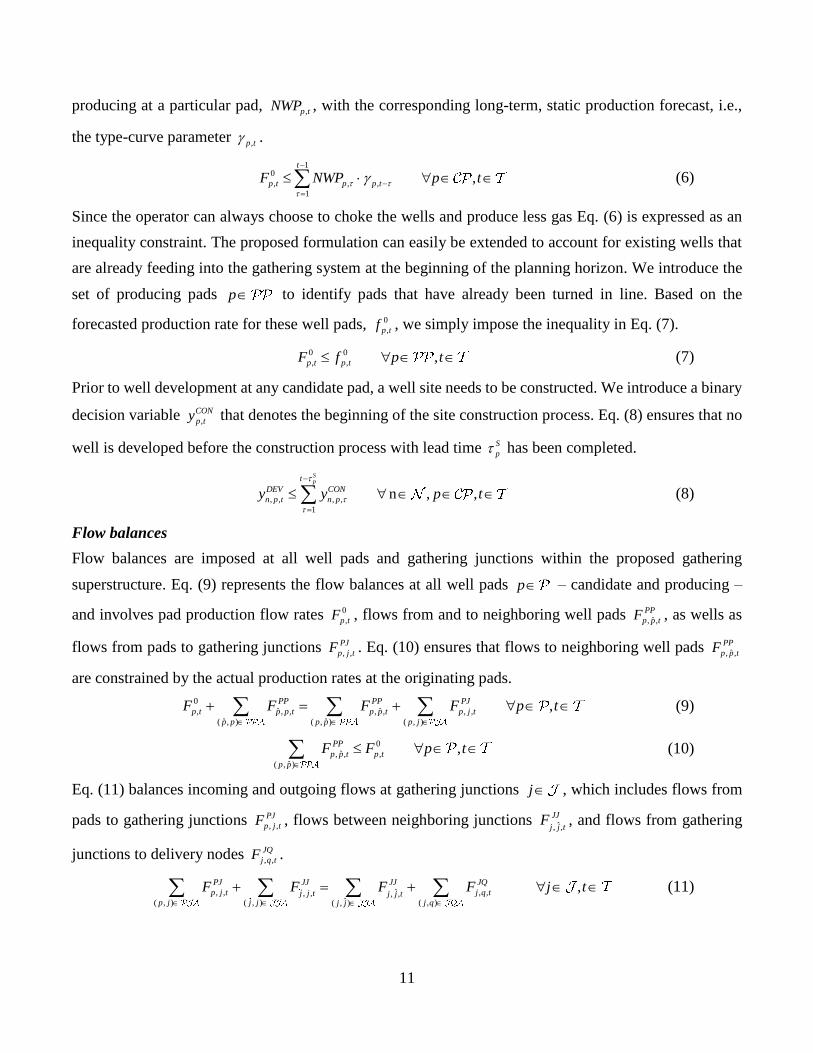
Production constraints
To determine how many horizontal wells n should be developed at every candidate pad p in
any time period t we introduce the binary decision variable , ,n p t
DRILLy . Since the development process
involves drilling, fracturing and completions operations, it will generally take several months after the
beginning of drilling operations until the wells have been completed and are ready for production. Hence,
we define the parameter D
n
W as the development lead time that increases with the number of wells being
developed in parallel. This parameter allows us to formulate Eq. (1), which states that the number of wells
that have been completed at a pad p in time period t , represented by the integer variable ,p tNWD
, depends on how many wells were drilled WD
nt time periods in advance, denoted by the binary variable
, , WDn
DRILL
n p ty
. It is important to note here that the number of wells
0n that can be drilled at a particular pad
location includes the zero-element 0n . Hence, the enforced multiple-choice constraint (2) can be satisfied
even when no wells are drilled.
0
, , ,,WD
n
DRIL
p t n p tn
LNWD n y p t
(1)
0
, ,t 1 ,n p
n
DRILLy p t
(2)
In practice the drilling and fracturing processes require different resources and cannot be performed
simultaneously. During the drilling phase, operators rely on tophole and horizontal rigs to drill the vertical
and lateral sections of the well. In preparation of the fracturing process, however, these rigs need to be
moved off the pad to free up space for roughly 12-18 tractor trailers equipped with high-power water
pumps that are eventually circled around each wellhead to fracture the wells. Hence, due to space
limitations, wells cannot be fractured while other wells are still being drilled and vice versa. This practical
constraint is expressed in Eq. (3) which states that as long any number of wells that have been drilled have
not been completed yet – captured by the development lead time parameter WD
n – no new set of wells can
be drilled.

10
, ,t , ,
1
1
1 ,WDn
DRILL
n p n p
n
tDRILL
n t
ty y p
(3)
The total number of wells that can be drilled and developed at every candidate location throughout the
planning horizon is generally constrained by the operator’s acreage position, permitting constraints, and/or
lease commencement and expiration dates. In the proposed formulation the parameter ,
max
p tn in Eq. (4) limits
how many wells can be developed at every candidate pad location at any point in time.
max
, ,
1
, ,DRILL
n
t
p pn ty n p tn
(4)
Upstream operators generally prefer to develop as many wells as possible at a particular well pad to take
advantage of economies of scale. To quickly recover their development expenses, the operators will
usually turn all completed wells in line as soon as possible, i.e., the extracted gas is fed into the gathering
system to downstream delivery nodes. However, given the characteristic shale well production profiles,
operators are increasingly exploring the option of keeping a subset of the developed wells shut-in
temporarily. The motivation for this strategy is as follows. Initially, shale well production rates are very
high, at times up to 280,000 m3/day. Turning all developed wells in line at the same time requires
substantial downstream capacity in terms of pipeline sizes and compression power. Such investments are
very costly, i.e., in the range of several million U.S. dollars, and within a matter of months the wells’
production rates will decline rapidly, often by as much as 65-85% within the first year after production
begin. At this time the previously installed downstream equipment is over-sized and under-utilized. To
avoid poor equipment utilization, operators may choose to keep a subset of the developed wells shut-in
temporarily and only produce from the remaining set of wells. In Eq. (5) we distinguish between the
number of wells that have been completed at a particular well pad, ,p tNWD , and the number of wells that
are actively producing, t
pNWP , thus allowing for temporary shut-ins.
, ,
1 1
,t t
p pNWP NWD p t
(5)
The implication of Eq. (5) is that the number of (active) wells producing raw gas is indeed an additional
degree of freedom to the optimization. The optimizer can choose to keep a subset of the developed wells
shut-in for any period of time to maximize equipment utilization, i.e., the available pipeline and
compressor capacity.
Based on how many wells are producing, we can calculate the amount of gas 0
,p tF that can be extracted at
every well pad at any point in time. This flow rate is obtained by multiplying the number of wells
11
producing at a particular pad, ,p tNWP , with the corresponding long-term, static production forecast, i.e.,
the type-curve parameter ,p t .
1
,,
0
,
1
,t
pp t p tNWP pF t
(6)
Since the operator can always choose to choke the wells and produce less gas Eq. (6) is expressed as an
inequality constraint. The proposed formulation can easily be extended to account for existing wells that
are already feeding into the gathering system at the beginning of the planning horizon. We introduce the
set of producing pads p to identify pads that have already been turned in line. Based on the
forecasted production rate for these well pads, 0
,p tf , we simply impose the inequality in Eq. (7).
0 0
,, ,p tp t f tF p (7)
Prior to well development at any candidate pad, a well site needs to be constructed. We introduce a binary
decision variable ,
N
p t
COy that denotes the beginning of the site construction process. Eq. (8) ensures that no
well is developed before the construction process with lead time S
p has been completed.
, ,, ,
1
n , ,
Spt
DEV C
n p
ON
n pt py ty
(8)
Flow balances
Flow balances are imposed at all well pads and gathering junctions within the proposed gathering
superstructure. Eq. (9) represents the flow balances at all well pads p – candidate and producing –
and involves pad production flow rates 0
,p tF , flows from and to neighboring well pads ˆ, ,p p
P
t
PF , as wells as
flows from pads to gathering junctions , ,
J
p j t
PF . Eq. (10) ensures that flows to neighboring well pads ˆ, ,p p
P
t
PF
are constrained by the actual production rates at the originating pads.
0
ˆ ˆ, , , , , ,
ˆ ˆ( , ) ( , ) (
,
, )
,p p t p p t p j t
p p p p p j
PP PP PJ
p t F F p tF F
(9)
0
ˆ, ,
ˆ,
,
( )
,PP
p t
p
p
p
p tF F p t
(10)
Eq. (11) balances incoming and outgoing flows at gathering junctions j , which includes flows from
pads to gathering junctions , ,
J
p j t
PF , flows between neighboring junctions ˆ, ,j j
J
t
JF , and flows from gathering
junctions to delivery nodes , ,
Q
j q t
JF .
ˆ
( , )
, , , ,, , , ,ˆ( , ) ( , ) ( , )
,p j t j q tj j t j j
PJ JJ J
t
J JQ
j qj j j jjp
F F F j tF
(11)

12
Equipment sizing constraints
The shale gas development problem requires operators to size necessary equipment such as pipelines and
compressors. In order to simplify the optimization problem the corresponding design variables are often
treated as continuous decision variables15. In practice, however, pipelines and compressors are
standardized in the oil and gas industry. Hence, we enforce discrete equipment sizes throughout this work,
i.e., we assume that only a finite set of pipeline diameters and compressor sizes are commercially
available. Moreover, for modeling purposes we take advantage of discrete equipment sizes by
systematically deriving disjunctive models based on Generalized Disjunctive Programming (GDP) that
generally yield tight continuous relaxations17. Lastly, in section Model Formulation: Objective Function
we show that by only considering discrete equipment sizes we can capture economies of scale without
explicitly having to introduce nonlinear, concave cost expressions into the objective function. We illustrate
the general equipment sizing framework proposed in this work with two examples, namely delivery
pipelines and gathering compressors.
Delivery pipelines are intended to connect gathering junctions j with delivery nodes q , and they
are a crucial part of any shale gas gathering system. Based on the proposed superstructure, the length of
candidate delivery pipelines, ,j ql , is known. Hence, the only remaining degree of freedom for sizing
purposes is the pipeline’s diameter. The more gas , ,
JQ
j q tF flows through a delivery pipeline segment, the
larger the respective pipeline diameter d needs to be to provide the right amount of flow capacity. In this
work we size pipelines based on fluid velocity, since pressure drops are relatively small in typical gas
gathering systems given that the pipeline segments are relatively short (< 15 km) and the operating
pressure is relatively low (< 2.5 MPa). In addition, gas velocity itself is an important design criterion that
is commonly used for preliminary sizing purposes. Operators need to bound the maximum gas velocity to
reduce noise emissions and prevent pipeline corrosion. Based on a pre-specified, maximum gas velocity,
we can calculate a sizing coefficient Pk that allows us to determine the necessary pipeline diameter with
sufficient accuracy. Details regarding the calculation of the sizing coefficient Pk are provided in Appendix
A: Pipeline Sizing.
Within the proposed model we use disjunction (12) to size delivery pipelines.
0
, , ,
20 2
, , ,
, ,d j q t
dP
PIPE
JQ
j q t j q d
jk F
qZ
t
(12)
0 , , , ( , ) ,PIP
d j q t
E
d j q tZ (13)
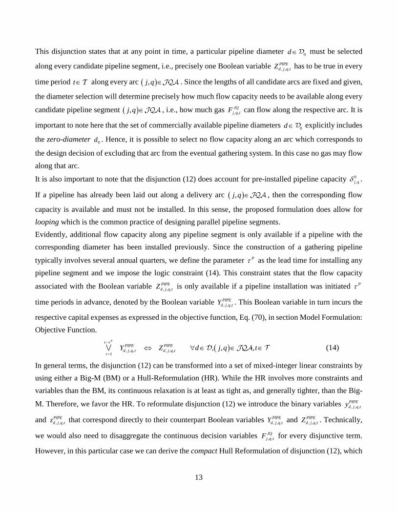
13
This disjunction states that at any point in time, a particular pipeline diameter 0d must be selected
along every candidate pipeline segment, i.e., precisely one Boolean variable , , ,d j q t
PIPEZ has to be true in every
time period t along every arc ,j q . Since the lengths of all candidate arcs are fixed and given,
the diameter selection will determine precisely how much flow capacity needs to be available along every
candidate pipeline segment ,j q , i.e., how much gas , ,
JQ
j q tF can flow along the respective arc. It is
important to note here that the set of commercially available pipeline diameters 0d explicitly includes
the zero-diameter 0d . Hence, it is possible to select no flow capacity along an arc which corresponds to
the design decision of excluding that arc from the eventual gathering system. In this case no gas may flow
along that arc.
It is also important to note that the disjunction (12) does account for pre-installed pipeline capacity 0
,j q .
If a pipeline has already been laid out along a delivery arc ,j q , then the corresponding flow
capacity is available and must not be installed. In this sense, the proposed formulation does allow for
looping which is the common practice of designing parallel pipeline segments.
Evidently, additional flow capacity along any pipeline segment is only available if a pipeline with the
corresponding diameter has been installed previously. Since the construction of a gathering pipeline
typically involves several annual quarters, we define the parameter P as the lead time for installing any
pipeline segment and we impose the logic constraint (14). This constraint states that the flow capacity
associated with the Boolean variable , , ,d j q t
PIPEZ is only available if a pipeline installation was initiated P
time periods in advance, denoted by the Boolean variable , , ,d j q t
PIPEY . This Boolean variable in turn incurs the
respective capital expenses as expressed in the objective function, Eq. (70), in section Model Formulation:
Objective Function.
, , , , , ,1
, , ,
P
d j q d j
tPIPE PIPE
q t d j q tY Z
(14)
In general terms, the disjunction (12) can be transformed into a set of mixed-integer linear constraints by
using either a Big-M (BM) or a Hull-Reformulation (HR). While the HR involves more constraints and
variables than the BM, its continuous relaxation is at least as tight as, and generally tighter, than the Big-
M. Therefore, we favor the HR. To reformulate disjunction (12) we introduce the binary variables , , ,d j q t
PIPEy
and , , ,d j q t
PIPEz that correspond directly to their counterpart Boolean variables , , ,d j q t
PIPEY and , , ,d j q t
PIPEZ . Technically,
we would also need to disaggregate the continuous decision variables , ,
Q
j q t
JF for every disjunctive term.
However, in this particular case we can derive the compact Hull Reformulation of disjunction (12), which

14
does not require disaggregated variables as shown in Appendix B: Compact Hull Reformulation. The
result is shown in Eq. (15).
The logic constraints (13) and (14) are transformed into the mixed-integer linear constraints (16) and (17)
using propositional logic. It should be noted that due to the structure of Eq. (17), either , , ,d j q t
PIPEy or , , ,d j q t
PIPEz
may be specified as continuous decision variables. In the authors’ experience, however, this does not yield
noticeable computational speed-ups.
0
20 2
, , , , , , , ,P
j q t j q d d j
JQ
q t
PIPE
d
k jF z q t
(15)
0
, , , 1 ( , ) ,PIPE
d j q t
d
z j q t
(16)
, , , , , ,
1
, , ,
P
PIPE PIPEt
d j q d j q tz d jy q t
(17)
The pipeline sizing formulation for delivery pipelines represented by Eqs. (15)-(17) is adapted for all
candidate gathering pipelines ˆ,j j , flow pipelines p, j and well pipelines p, p
that are considered in the gathering superstructure. In addition, Eqs. (18) and (19) are redundant constraints
that enforced to strengthen the pipeline sizing formulation.
0 0
, , , , , , , ,( , , ) ,p j d p j t d dj j d j j
PIPE PIPE
dt
d
y j ty p j
(18)
0 0
ˆ ˆ, , , , , , , ,ˆ( , , ) ,PIPE PIPE
d d
d dj j d j j t j j d j j tj j jy y t
(19)
The underlying logic is that prior to solving the shale gas development problem, operators can easily
identify non-decreasing pipeline capacity arcs , , jp j and ˆ,, j jj within the gathering
superstructure. Along these neighboring arcs, the flow capacity – represented by the installed pipeline
capacity – is not allowed to decrease, i.e., a decrease in flow capacity would indicate that the preceding
pipeline segment is over-sized. If two pipelines merge into one segment, for example, it is clear that the
subsequent pipeline may not decrease in terms of flow capacity. In practice, similar constraints are
oftentimes imposed as part of the design problem to allow for “pigging” in gathering pipelines, i.e., the
practice of using so-called “pigs” to clean operational pipelines in regular intervals.
The proposed sizing formulation for pipelines can easily be extended to size gathering compressors. These
compressors need to be installed between regional shale gas gathering systems and interstate transmission
pipelines. Typically, the line pressure of shale gas gathering systems is in the range of 2 MPa, whereas
interstate transmission pipelines are generally operated at well above 7 MPa. Operators are only
responsible for installing gathering compressors along direct delivery sales routes, i.e., when gas
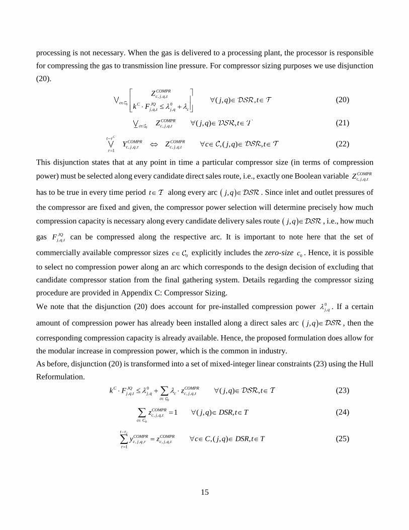
15
processing is not necessary. When the gas is delivered to a processing plant, the processor is responsible
for compressing the gas to transmission line pressure. For compressor sizing purposes we use disjunction
(20).
0
, , ,
0
, , ,
( , ) ,
COMPR
c j q t
c C
j q t c
JQ
j q
j q tk
Z
F
(20)
0 , , , ( , ) ,COMP
c c j q t
R j q tZ (21)
, , , , , ,1
,( , ) ,
Ct
c j q c j q t
COMPR COMPRY cZ j q t
(22)
This disjunction states that at any point in time a particular compressor size (in terms of compression
power) must be selected along every candidate direct sales route, i.e., exactly one Boolean variable c, , ,
C
q
R
j t
OMPZ
has to be true in every time period t along every arc ,j q . Since inlet and outlet pressures of
the compressor are fixed and given, the compressor power selection will determine precisely how much
compression capacity is necessary along every candidate delivery sales route ,j q , i.e., how much
gas , ,
JQ
j q tF can be compressed along the respective arc. It is important to note here that the set of
commercially available compressor sizes 0c explicitly includes the zero-size
0c . Hence, it is possible
to select no compression power along an arc which corresponds to the design decision of excluding that
candidate compressor station from the final gathering system. Details regarding the compressor sizing
procedure are provided in Appendix C: Compressor Sizing.
We note that the disjunction (20) does account for pre-installed compression power 0
,j q . If a certain
amount of compression power has already been installed along a direct sales arc ,j q , then the
corresponding compression capacity is already available. Hence, the proposed formulation does allow for
the modular increase in compression power, which is the common in industry.
As before, disjunction (20) is transformed into a set of mixed-integer linear constraints (23) using the Hull
Reformulation.
0
0
, , , , , , ( , ) ,JQ COMPRC
j q t j q c c j q t
c
k z j qF t
(23)
0
, , , 1 ( , ) ,COM R
c
P
c j q t
C
z j q DSR t T
(24)
, , , , , ,
1
,( , ) ,c
COMPR COMPRt
c j q c j q tz c C j q S t Ty D R
(25)

16
In this case the previously introduced binary variables , , ,
C
c j
R
q t
OMPy and , , ,
C
c j
R
q t
OMPz correspond directly to their
counterpart Boolean variables , , ,
C
c j
R
q t
OMPY and , , ,
C
c j
R
q t
OMPZ . Here, too, the introduction of disaggregated variables
and the corresponding constraints can be avoided as shown in Appendix B: Compact Hull Reformulation.
Thus Eq. (23) represents the compact Hull Reformulation of disjunction (20). The logic constraints (21)
and (22) are transformed into the mixed-integer linear constraints (24) and (25) using propositional logic.
Water management constraints
Hydraulic fracturing of horizontal wells requires large amounts of fracturing fluid, oftentimes several
million liters of water per well. Hence, it must be ensured that the demand for water can be met by the
available set of water supply sources. In this work it is assumed that the water demand for fracturing is
given in terms of the location-specific parameter pfwd .
, , , , ,n p
DEV
t f p t
f
p
n
fwd y Fn WS p t
(26)
Constraint (26) ensures that the water supply , ,f p tFWS from the available set of water sources f
satisfies the water demand at every well pad, depending on how many wells are being developed in
parallel. In turn, constraint (27) balances the water supplied to all well pads with the water availability at
all water sources, given by the parameter ,f tfwa .
, , , ,f p t f t
p
FWS fwa f t
(27)
Rig and crew allocation constraints
In practice upstream operators generally only have a limited set of drilling rigs and completion crews at
their disposal in a particular development area. The allocation of these resources is a challenging and
complicating factor in the planning process. Hence, we introduce a binary decision variable , ,r p
G
t
RIy that is
active if a drilling rig and completion crew r are present at a candidate pad location p in time
period t . Constraint (28) ensures that a drilling rig and completion crew are on site for as long as any
number of wells are being developed at a candidate pad location. A drilling rig and completion crew may
not be assigned to more than one well pad at any time as expressed by Eq. (29).
, , , ,
1
,
nDR
tDRILL
n p r p t
RIG
n rt
y y p t
(28)
, , 1 ,RI
p t
G
r
p
y tr
(29)
Strategic development constraints
In practice, upstream operators oftentimes have the flexibility to choose from a set of candidate delivery
nodes that are within the vicinity of their gathering system. These take-away options range from direct

17
taps into nearby interstate transmission pipelines to processing plants that purify the raw gas prior to its
injection into a transmission system. In addition to selecting the preferred delivery node, the operators
also need to determine what kind of delivery agreements to arrange and how much delivery capacity to
procure. The arrangement of these agreements is a quality-sensitive and nontrivial aspect of the overall
long-term shale gas development problem.
In this section we define the constraints that govern the strategic selection of: a) a preferred delivery node,
b) delivery agreements, and c) necessary delivery or “take-away” capacity. Fig. 5 illustrates these three
levels of strategic decisions and the particular categories of constraints that they involve. The proposed
formulation for the incorporation of strategic development constraints is motivated by Park et al.18 who
include the selection of different types of contracts into existing supply chain optimization models using
disjunctive programming. However, whereas Park et al. focus on generic purchasing and sales contracts
between suppliers and customers, our models are tailored to the unique structure of the natural gas
industry.
In this work we capture the corresponding strategic development constraints using disjunction (30). This
disjunction itself is characterized by a set of embedded disjunctions, and thus exploits the inherent
structure of the strategic decision-making process.
,
max
, , , ,
0 max
, ,
max
, , , ,
min max
, , , , , , , , ,
, ,
,
, ,
,
, , ,
, ,
DEL
j q
j q t j q t
j q t
p
j q t j q t
j q
JQ
p t
JQ KJQ J
t j q k j
Q
k
q t k j q t j q
AGR
da j q
j q
j q t da k j
j q t da
d
PR KJQ
t
EV
a
q
R
f t
f t
REV rev t
F h h F h t
PRE F
Y
F
F
F
Y
f
REV f
t
, , ,
, , , ,
, , , , ,
, , , , , , ,
min max
, , , , , , , , , , , , ,
KJQ
CPTY
JQ
JQ S
JQ KJQ JQ
k j q t
dc da j q t
j q t dc da j q
dcdc da j q j q t j q t
j q t dc da j q k j q t k j q t dc da q
k
j
t
F t
F t
F h h
F
F
F h
Z
F t
(30)
At the highest level, upstream operators have to select their preferred delivery node for a particular
gathering system. This selection is of significant importance as it can vary between two conceptually
disparate delivery options: processing sales routes and transmission sales routes. Whereas processing

18
plants along processing sales routes ( , )j q are designed to purify off-spec raw gas deliveries,
transmission lines along direct sales routes ( , )j q generally only accept pipeline-quality gas
deliveries. This diversity in terms of delivery options can be interpreted as a strategic degree of freedom
to the upstream operator providing the decision-makers with a certain degree of flexibility. On the other
hand, the conditions and terms of each delivery option also complicate long-term strategic commitments
and add to the challenge of the development problem.
The Boolean variable ,
DEL
j qY controls the outermost disjunction (30) and allows for the selection of a
particular delivery arc ( , )j q . This selection bounds the maximum take-away capacity max
, ,j q tf , the
maximum attainable revenues , ,
max
j q trev and it imposes gas quality specification constraints in terms of the
heating value of the gas delivery ,
min
j qh and ,
max
j qh . In this section we assume for simplicity that the delivery
node selection may only be made once throughout the planning horizon. Hence, the logic constraint (31)
applies. The relaxation of this restriction is discussed in section Model Formulation: Multiple Delivery
Node Problem.
,,
DEL
j qj qY
(31)
Besides the selection of a preferred take-away node, upstream operators must also choose from a limited
set of delivery agreement options they are offered. In terms of processing plants, for example, these
contracts range from fee-based to percent-of-proceeds and keep-whole processing agreements19. These
agreements are conceptually different with regards to how the upstream operator compensates the
processor for the processing service, and how revenues are generated for either party. Under fee-based
contracts the operator simply pays a volume-based fee for the processing service, under percent-of-
proceeds contracts the operator and the processor split revenues from marketing the gas and extracted
NGLs, and under keep-whole contracts the processor retains title to all extracted NGLs as a method of
payment. In addition, every possible delivery agreement may involve further specific terms and conditions
regarding contract durations, delivery capacities or gas quality specifications. Delivery agreement options
along direct sales routes are generally limited but may vary as well.
In this work, we embed the selection of the optimal delivery agreement within disjunction (30). For this
purpose we introduce the Boolean variable , ,
AGR
da j qY which is true if a particular delivery agreement da DA
is arranged along a take-away arc ( , )j q . This selection will determine the form of the processing
cost function , , ,( )da k j q t
PR KJQf F and the revenue function , , ,( )da k j q t
REV KJQFf . Constraint (32) ensures that if the
Boolean variable ,
DEL
j qY is true, i.e., a particular take-away node has been selected, then one of the available
19
delivery agreements needs to be arranged, i.e., a corresponding Boolean variable , ,
AGR
da j qY has to be true, too.
The reverse statement holds true as well.
, , , ( , )DEL AGR
j q da jda
qY j qY
(32)
In addition, the logic constraints (33) and (34) are imposed to explicitly distinguish between processing
agreements and transmission agreements that operators may enter into depending on which type of
delivery node is selected. The set of processing agreements pa and transmission agreements
ta complement the set of delivery agreements da DA . Constraint (33) expresses that if a delivery
node among the set of processing sales routes ( , )j q is selected, then one of the available processing
agreements pa has to be arranged. Vice versa, constraint (34) states that deliveries along
transmission sales routes ( , )j q must be governed by one of available the transmission agreements
ta .
, , , ( , )DEL AGR
j q pq jpa
qY j qY
(33)
, , , ( , )DEL AGR
j q ta jta
qY j qY
(34)
Due to the complexity of the bilateral negotiation process between upstream operators and downstream
entities, we assume that the arrangement of any delivery agreement may only be made once throughout
the planning horizon. This is enforced by constraint (35).
, , ( , )AGR
da da j q j qY (35)
Finally, upstream operators have to determine how much delivery capacity to request at a particular
delivery node. Generally, only discrete increments of take-away capacity can be procured, typically
classified as limited, average, or extended delivery capacity. The more delivery capacity an upstream
operator wishes to secure, the longer the duration of an agreement tends to be. Downstream entities,
including processing plants and transmission lines, will specify minimum delivery quantities for the
duration of a delivery agreement to ensure that they can recover their expenses for providing take-away
capacity. Commonly, these minimum delivery clauses involve so-called take-or-pay provisions that
obligate the upstream operator to either deliver the specified quantity, i.e., “take” the capacity, or to
compensate the delivery entity, i.e., “pay” for unutilized capacity. Depending on how much take-away
capacity is requested, additional and more restrictive gas quality specifications may be imposed as well.
A midstream processor, for example, may offer limited processing capacity over a short period of time
provided the delivered gas meets strict quality specifications.

20
Within the embedded, innermost delivery capacity selection disjunction (30) we introduce the Boolean
variable , , , ,
CPTY
dc da j q tZ which is true if delivery capacity dc is available as part of delivery agreement
da along delivery arc ( , )j q in time period t . If this Boolean variable is true, then the
gas flowrate , ,
Q
j q t
JF along the corresponding delivery arc is bounded by the maximum delivery quantity
parameter , , ,dc da j q . In addition, a minimum delivery quantity restriction , , ,dc da j q may apply. Given the
characteristic shale well decline curves these minimum delivery restrictions can be especially challenging
to meet. In order to ensure a steady supply of natural gas, operators will generally try to turn new wells in
line continuously. In this context we account for common take-or-pay provisions by introducing the slack
variable , ,
S
j q tF . This variable closes the gap between the actually delivered gas flow , ,
Q
j q t
JF and the arranged
minimum delivery quantity , , ,dc da j q . As such, the slack variable , ,
S
j q tF represents procured but unutilized
capacity. Finally, the embedded delivery capacity selection disjunction involves the aforementioned gas
quality specifications , , ,
min
dc da j qh and , , ,
max
dc da j qh that may or may not apply.
The logic constraint (36) guarantees that delivery capacity is available whenever a particular delivery
agreement is selected and vice versa. This constraint links the agreement selection disjunction with the
embedded capacity selection disjunction.
, , , , , , ,( , ) ,AGR
da j q dc da j q t
CPTY
dc
Z daY j q t
(36)
Similar to the case of delivery agreements, we distinguish between delivery capacity in terms of
processing capacity and transmission capacity. Increments of processing capacity pc are only
available along processing sales routes ( , )j q as part of processing agreements pa , whereas
transmission capacity increments tc are restricted to transmission agreements ta along
transmission sales routes ( , )j q . The logic constraints (37) and (38) establish these links among the
embedded delivery agreement and delivery capacity selection disjunctions.
, , , , , , ,( , ) ,AGR CPTY
pa j q pc pa j qpc
tZ pa j qY t
(37)
, , , , , , ,( , ) ,AGR CPTY
ta j q tc ta j qtc
tZ ta j qY t
(38)
We define the parameter ,
A
dc da that specifies the agreement length for delivery capacity dc under
delivery agreement da . We also introduce the Boolean variable , , , ,
CPTY
dc da j q tY that represents the selection
of delivery capacity dc as part of delivery agreement da along delivery arc ( , )j q in
time period t , i.e., this Boolean variable marks the beginning of the capacity availability. Based on
this variable declaration, constraint (39) states that delivery capacity, denoted by the Boolean variable
21
, , , ,
CPTY
dc da j q tZ , is only available as long as the beginning of the arrangement occurred within the previous ,
A
dc da
time periods. During this time, all corresponding restrictions including minimum delivery quantities and
gas quality specifications apply.
,
, , , , , , , , , ,( , ) ,Adc da
tCPTY
dc da j q dc da j q
CPTY
tt
Y dc da jZ q t
(39)
Finally, constraint (40) ensures that some increment of delivery capacity is available along every delivery
arc ( , )j q at any point in time. Technically, however, the set of available delivery capacities
dc will always involve a zero-capacity element 0dc .
, , , , ,( , ) ,CPTY
dc dc da j q t da j q tZ (40)
In this work the disjunctions are reformulated as mixed-integer linear constraints using both the big-M
and the Hull Reformulation. For this purpose we introduce the binary variables ,
DEL
j qy , , ,
AGR
da j qy , , , , ,
CPTY
dc da j q ty and
, , , ,
CPTY
dc da j q tz that correspond directly to the respective Boolean variables defined previously.
The outer disjunction (30) capturing the delivery node selection is transformed into a set of mixed-integer
linear constraints using the Hull Reformulation. This disjunction involves the continuous decision
variables , ,
Q
j q t
JF , , , ,k j q
Q
t
KJF , , ,j q tREV and 0
,p tF . In this case only the latter variable needs to be disaggregated as
0
, , ,p j q tF for each disjunctive term ( , )j q as expressed in constraint (41).
,
( , )
0 0
, , , ,p j q tp t
j q
pF F t
(41)
For the special case of the single delivery node problem, we can take advantage of the disaggregated
variable 0
, , ,p j q tF when imposing the component flow balance Eq. (42).
0 0
, , , , j, , , ,( , ) ,k
KJQ
j q t p q t p k
p
F x k j q tF
(42)
The reasoning for this constraint is as follows: by “design” the single delivery node problem forces all
flows to converge to one delivery node eventually, i.e., regardless of the final design of the gathering
system all of the gas that is extracted within the development area will be delivered to one and the same
take-away hub. Since the composition of the extracted gas 0
,p kx is known at every well pad, we can enforce
constraint (42), which balances how much of each component k is produced at all well pads in every
time period with the component flow to all available delivery nodes. This explains why the single delivery
node problem can indeed be solved as a mixed-integer linear program.
In addition, we impose the upper and lower bound constraints (43)-(46) for all decision variables involved
in the outer disjunction.
22
0 max
, , , , , ,0 , ,p j q t j q
L
t
DE
j qf y j q tF (43)
max
, , , , ,0 ( , ) ,DEL
j q t j q t j
J
q
QF f y j q t (44)
max
, , , , , , ,0 ( , ) ,DEL
k j q t k j q t
Q
j
K
q
JF f y j q t (45)
max
, , , , ,0 ( , ) ,DEL
j q t j q t j qREV rev y j q t (46)
We note here that constraints (41) and (43) are not absolutely necessary, but are rather imposed to tighten
the formulation. The gas quality specification constraint is adopted directly as it holds regardless of which
disjunctive term is active.
min max
, , , , , , , , ,j q t j q k j q t k j q t
JQ KJQ JQ
k
j qF h h F h tF
(47)
Constraint (48) ensures that only one node may be selected for delivery, i.e., only one term can be active
in the outer disjunction (30).
,
,
1DEL
j
q
q
j
y
(48)
The logic link (32) between the outer delivery node selection disjunction and the embedded center
disjunction concerning agreement arrangements is reformulated into the algebraic constraint (49). The
same transformation holds for the specialized logic propositions (33) and (34) affecting deliveries along
processing and transmission sales routes.
, , , ( , )DEL AGR
d
j q da j q
a
j qy y
(49)
, , , ( , )DEL AGR
p
j q pa j q
a
j qy y
(50)
, , , ( , )DEL AGR
t
j q ta j q
a
j qy y
(51)
The constraints within the embedded center disjunction itself are converted into mixed-integer linear
constraints using a big-M reformulation. For this purpose we define the big-M parameters , ,
PRE
da j qm and
, ,
REV
da j qm . Depending on which agreement type da is selected, i.e., which binary variable , ,
AGR
da j qy is
active, determines which processing expenses accrue and how revenues are generated. At this point we
review the most common types of delivery agreements in more detail, i.e., fee-based, percent-of-proceeds,
keep-whole, and direct delivery contracts and we present the corresponding processing and revenue
functions.
Fee-based processing agreements (index da FB ) are the most common arrangements between upstream
operators and midstream processors. Under these, operators pay a service fee A
FB to the processor based
on how much gas is processed in terms of throughput volumes. Eq. (52) captures the processing expenses

23
, ,j q tPRE under such a fee-based agreement. In return, the processor receives all pipeline-quality gas and
any natural gas liquids extracted from the raw gas stream to the operator who markets these. Eq. (53)
shows the operator’s revenue function.
, , FB, ,, , , , , ,1 ( , ) ,JQ S PRE
q t j q
A AGR
FB j j q t j q t FB j qF PRE m y j qF t (52)
, , , FB, ,, , , , , ,1 ( , ) ,KJQ REV
k j q t j q
AGR
j q t q k t FB j q
k
p m y j qV F tRE
(53)
Under fee-based processing contracts the processor’s revenues are primarily related to the quantity and
not the quality of the gas that is delivered. To the operators, on the other hand, who market the gas and
liquids exclusively, these arrangements are highly quality-sensitive; when NGL prices are high,
processing can increase the operator’s overall revenues, whereas low NGL prices favor other alternative
agreements or blending strategies to reduce or avoid the need for processing.
Under percent-of-proceeds contracts (index da PP ) processors will generally only charge a small
servicing fee A
PP for their processing service depending on how much gas is received. These processing
expenses are captured by Eq. (54). In addition, however, the processors are entitled to receive an agreed
upon percentage PP of the proceeds from all natural gas and NGLs sales19. Hence, upstream operators
and midstream processors split the overall revenues. Therefore, the operator’s revenues are given by Eq.
(55). Under percent-of-proceeds arrangements both parties, the operators and the processor, share
commodity risks.
, , PP, ,, , , , , ,1 ( , ) ,JQ S PRE
q t j q
A AGR
PP j j q t j q t PP j qF PRE m y j qF t (54)
PP, , , , , , , ,, ,, 1 ( , )1 ,AGR
j q t PP k j q t q k
KJQ REV
j qt PP
k
j qp m y j tE qR V F
(55)
Under keep-whole arrangements (index da KW ) the midstream processor is compensated for the
processing service by retaining title to any NGLs recovered from the raw gas stream. In return, the
upstream operator receives an identical amount of pipeline-quality gas that equals the heating value of the
original raw gas stream. Thus, the operator is “kept whole” on a heating value basis. Since the processors
market the NGLs exclusively under keep-whole agreements, they are directly exposed to NGL price
fluctuations, which presents a severe strategic risk. However, when NGL prices are high, midstream
processors can generate substantial revenues from these contracts. The corresponding constraints are as
follows:
, , KW, ,, , , , , ,1 ( , ) ,JQ S PRE
q t j q
A AGR
KW j j q t j q t KW j qF PRE m y j qF t (56)
, , , , , KW, ,, 4, , ,
4
1 ( , ) ,KJQ REV
j q
k
AGRkj q t k j q t q CH t KW j q
CH
HREV
HF p m y j q t
(57)

24
Direct deliveries contracts (index da DD ) generally do not imply significant processing expenses, and
hence, the processing cost coefficient A
DD in Eq. (58) is usually set to zero. In rare cases, though,
transmission companies may impose a minimum fee for dehydrating the received gas. Either way, the
operator gets to market all gas and natural gas liquids sales individually as depicted in Eq. (59).
, , DD, ,, , , , , ,1 ( , ) ,JQ S PRE
q t j q
A AGR
DD j j q t j q t DD j qF PRE m y j qF t (58)
DD, , , , , 4, , ,,, , 1 ( , ) ,AGR
j q t k j q t q C
KJQ REV
j q
k
H t DD j qRE F p m y j q tV
(59)
Constraint (60) states the general expression for processing expenses where the processing cost coefficient
A
da changes depending on which type of agreement is selected.
, , , , ,, , da ,, , 1 ,( , ) ,JQ S PRE
q t j q
A AGR
da j j q t j q t da j qF PRE m y j q tF da (60)
The functional form of the revenue expression changes depending on which agreement is arranged
between an upstream operator and a processing plant, for example. We note that processing expenses
accrue for delivered gas volumes, , ,
Q
j q t
JF , and for procured, but unutilized processing capacity, , ,
S
j q tF .
Constraint (61) ensures that only one particular delivery agreement can be selected along every delivery
arc ( , )j q .
, , (1 , )AGR
a
da
d j q j qY
(61)
We link the embedded center and innermost disjunctions through constraint (62) that corresponds to the
logical proposition (36). As before, this transformation also holds for the specialized logic propositions
(37) and (38) addressing processing and transmission agreements.
, , , , , , ,( , ) ,AGR CPTY
da j q dc da j
dc
q t da j qy z t
(62)
, , , , , , ,( , ) ,AGR CPTY
pa j q pc pa j
pc
q t pa j qy z t
(63)
, , , , , , ,( , ) ,AGR CPTY
ta j q tc ta j
tc
q t ta j qy z t
(64)
The embedded innermost disjunction in (30) capturing the delivery capacity selection is converted into
algebraic constraints by using a big-M reformulation. The constraints involved in this disjunction address
minimum delivery restrictions, capacity constraints, and gas quality specifications. By introducing
sufficiently large parameters , , ,dc da j qm , , , ,dc da j qm , , , ,
minh
dc da j qm and , , ,
maxh
dc da j qm we can derive the big-M constraints
(65)-(68), respectively.
, , , , , , , , , , , , , ,1
, ,( , ) ,
CPTY
dc da j q j q t j q t dc da j q dc da j q t
JQ SF z
dc da j q
F
t
m
(65)

25
, , , , , , , , , , , ,1
, ,( , ) ,
j q t dc da j q dc da j q dc d
JQ CPTY
a j q tmF z
dc da j q t
(66)
min
, , , , j, , , , , , , , , , ,1
, ,( , ) ,
minh
j q t dc da q k j q t k dc da j q dc da j
JQ KJQ CP
q
k
t
TYF h F h z
dc da j q t
m
(67)
max
, , , , , , , j, , , , , , , ,1
, ,( , ) ,
maxh
k j q t k j q t dc da q dc da j q dc da j
KJQ JQ CP
q
k
t
TYF h h z
dc
F
da q
m
j t
(68)
Finally, the logic proposition (39) governing the length of delivery capacity agreements is reformulated
as constraint (69).
,
, , , , , , , , , ,( , ) ,Ada da
CPTY
dc da j q dc da j q t
tCPT
t
Y z dc da j q ty
(69)
Model Formulation: Objective Function
The objective for shale gas development from the operator’s perspective is to maximize the net present
value (NPV) over an extended planning horizon. The proposed objective function (70) accounts for
revenues from natural gas and natural gas liquids sales tREV , development expenses
tDVE , installation
expenses for flow pipelines tFPE , gathering pipelines
tGPE , delivery pipelines tDPE , compressor
installation expenses tCIE , compressor operating expenses
tCOE , production and maintenance expenses
tPME , water acquisition expenses tFWE , royalty payments
tRRE , rig transition expenses tRTE , rig
downtime expenses tRDE , site construction expenses
tSCE and processing expenses tPRE .
0
, ,T t ,
max (1 ) t
t
t t t t t t
t t t t t t t t
p t p p k
t pT k
k
P K
dr
FPE GPE DPE CIE
COE PME FWE
NPV
REV DVE
RRE RTE RDE SCE PRE
NWP x p
(70)
The last term in the objective function (70) captures the terminal value of the development project. Since
the wells are expected to produce many years beyond the explicit planning horizon these revenues need
to be factored into the net present value. For this purpose we consider the number of wells that are turned
in-line at every pad in every time period ,p tNWP , the expected, discounted, cumulative production of a
well beyond the explicit planning horizon ,p T t , the gas composition 0
,p kx , and an expected price forecast
beyond the explicit planning horizon for every gas component kp . Assuming that the implicit planning

26
horizon extends to time period t T we determine the expected, discounted cumulative production of a
well beyond the explicit planning horizon as follows:
1
, , 1T t
t
p T t p
T t
dr
(71)
The overall revenues tREV are driven by natural gas and NGLs sales along the delivery sales routes
( , )j q as outlined in constraint (72). The explicit expressions for individual revenue streams along
particular sales routes , ,j q tREV are given by constraints (53)-(59) above as they depend on the arrangement
of particular processing agreements.
(
,
, )
,
j q
t j q tREV tREV
(72)
Economies of scale play a crucial role in shale gas development since the major capital investment
expenses for drilling wells, laying out pipelines and installing compressor stations are well-known to obey
these scaling principles20,21,22. Dawson et al.23 go as far as to argue that the success or failure of
unconventional gas development hinges upon the principles of economies of scale.
Commonly, economies of scale are captured by concave investment cost functions of the form,
( 0 1) xf x
where ( )f x are the equipment cost, x represents the equipment size, and finally and are cost
parameters. The design variable x , i.e., the equipment size such as the pipeline diameter or compression
power is commonly treated as a continuous variable15. However, due to the concave nature of the cost
function above, these expressions can give rise to multiple local optima and unbounded gradients at zero
values for equipment sizes ( 0x ), leading to failures in NLP algorithms. Moreover, a posteriori rounding
of equipment sizes can lead to suboptimal or even infeasible solutions.
We overcome these difficulties by taking advantage of the discrete nature of the design variables involved
in the shale gas development problem. Since pipeline diameters and compressor sizes are standardized in
practice, we restrict the respective design variables to a finite set of discrete values 1 2{ , , , }i Nx xx x (as
shown in Fig. 6) and introduce binary variables {0,1}iy to select the optimal equipment sizes. This
allows us to derive the following mixed-integer linear constraints for investment costs that are subject to
economies of scale.
1
)( i i i
N
i
x yf y
1
1N
i
iy

27
The important feature of the proposed reformulation is that it readily allows the consideration of discrete
sizes and that it avoids nonlinear cost terms in the objective function due to economies of scale. However,
depending on the number of discrete sizes, a large number of binary variables may be introduced that
could render the mixed-integer programs expensive to solve. But even though the revised formulation is
significantly larger in terms of discrete variables, it does yield a number of advantages: a) the simplified
treatment of discrete equipment sizes as continuous variables is avoided, b) à posteriori rounding of
equipment sizes is no longer necessary, and c) economies of scale can be accounted for without having to
introduce nonlinear, concave cost functions into the objective function.
In terms of the proposed model, we assume that expenses related to well developments as well as pipeline
and compressor installations are subject to economies of scale. Hence, the respective cost expressions
correspond to the modified cost function. Regarding well development expenses, for instance, the number
of wells that can be drilled at any candidate pad location is an element of the discrete set n . By
defining the cost parameters D and D we can take advantage of the previously introduced binary
variable , ,
DEV
n p ty and express the development expenses using constraint (73). This expression is linear even
though it captures the nonlinear nature of economies of scale.
, ,
DD DRILL
t n p t
p n
DVE n y t
(73)
The same procedure can be applied to investment costs arising from the installation of delivery, gathering,
flow and well pipelines. In all four cases we rely on the corresponding binary variables , , ,d j q t
PIPEy , ˆ, , ,d j j
E
t
PIPy ,
, , ,d p j t
PIPEy and ˆ, , ,d p p
E
t
PIPy to derive the cost expressions (74)-(76).
, , , ,
( , )
PP
t j q d d j
PIPE
q t
j q d
DPE tl y
(74)
ˆ ˆ, , , ,ˆ( , )
PP
t dj j d j j td
PIPE
j j
GPE l y t
(75)
ˆ ˆ, , , , , , , ,
ˆ( , ) ( , )
P PIPP
t d p j d p j t p p d p p t
d p j p p
E PIPEFPE l y l y t
(76)
The constraints involve the cost parameters P and P as well as the lengths of candidate pipeline
segments ,j ql , ˆ,j jl , ,p jl and ˆ,p pl . The parameter
d stands for commercially available pipeline diameters
and is linked to the elements of the set d .
Expenses related to the installation of compression power are captured in a similar fashion. We assume
that compressors only need to be installed along direct sales routes ( , )j q leading to interstate

28
transmission pipelines. We define the parameter c to represent commercially available compressor sizes
c and use the cost parameters C and C to describe the characteristic economies of scale.
Consequently, the selection of a particular compressor size, denoted by the binary variable , , ,
C
c j
R
q t
OMPy ,
determines the compressor installation expenses as given by expression (77).
,
( , )
, ,
CC COMPR
t c c j q t
cj q
CIE y t
(77)
Expenses for the operation of compressors as well as other production and maintenance costs, are captured
by Eqs. (78) and (79). For simplicity we assume that compression expenses are directly proportional to
the gas flow through the respective compressors. Similarly, production and maintenance expenses depend
primarily on how much gas is extracted at all well pads within the development area.
, ,
( , )
JQ
q
j
O
t j t
q
COE F t
(78)
,
0
p t
I
t
p
PME F t
(79)
In many U.S. states minimum royalty rates are prescribed by law and set to approximately 13% of the
value of the extracted oil or gas. In this work we introduce a parameter to represent the royalty rate prr
and impose the expression (80).
0
,
0
,
0
,p t k tt p pk
kp
RRE nd p tx rF r
(80)
Freshwater acquisition expenses for fracturing operations are described by Eq. (81). We define the cost
parameter W and assume that the cost of water acquisition is proportional to the amount of water that is
required, , ,f p tWS , and the distance between a water source and the well pad ,f pl .
, , ,
W
t f p f p t
f p
FWE l WS t
(81)
In practice, significant expenses accrue whenever a drilling rig is moved from one well pad to another.
These are mainly due to the costly assembly and disassembly of the rigs. We define the rig transition cost
parameter R and assume that transition expenses accumulate whenever a drilling rig is either assembled
or disassembled at a well pad. Since the binary variable , ,r p
G
t
RIy identifies whether a drilling rig is located at
a particular well pad or not, we use constraint (82) to anticipate rig transition expenses. The proposed
constraints (82) - (84) are derived from the reformulation of the absolute value , ,r p tRTE .
29
, , , , , , , ,t 1(y - ) , ,R
r p t r p t r p t
RIG RIG
r pRTE RT tE pY r
(82)
, , , ,, 0 , ,r p t r p tRT RTE tE r p (83)
, , , ,t r p t r p t
r p
RTE RTERTE t
(84)
Usually, upstream operators will enter servicing agreements with rig companies and lease drilling rigs
over several years. Under these agreements, the upstream operators are typically required to compensate
the rig companies even when their services are not needed. These so-called rig downtime expenses are on
the order of $50,000 per day, and hence contribute significantly to the overall development expenses. We
account for rig downtime expenses tRDE in Eq. (85).
, , , ,DRn
tRIG DRILL RD
t r p t n
p r p n
p
t
RDE ty y
(85)
For as long as the employed number of rigs are drilling on a well pad – captured by an active binary
variable , ,t
DRILL
n py and the drilling lead time parameter DR
n – no expenses accrue. For any rig that is not
involved in drilling operations in time period t the rig downtime expense RD applies.
The construction of a well site may take place several months prior to the beginning of drilling operations.
Based on the site construction cost coefficient S and the binary variable ,
CON
p ty – which marks the begin
of construction operations – we calculate the site construction expenses tSCE using constraint (86).
, ,
CONS
t n
p
n p t
n
SCE y t
(86)
Processing expenses accrue only along processing sales routes ( , )j q and depend on what type of
processing agreement is arranged. Constraint (87) accounts for processing expenses along all candidate
processing arcs. The individual processing expenses , ,j q tPRE are captured by constraints (52)-(58).
(
,
, )
,
j q
t j q tPRE PRE t
(87)
In conclusion, the proposed model for the single delivery node development problem is composed of
constraints (1)-(87). Since these constraints consist solely of mixed-integer linear constraints, the
suggested formulation corresponds to an MILP that can be solved to global optimality.
Model Formulation: Multiple Delivery Node Problem
The previously proposed formulation for the single delivery node development problem can easily be
extended to account for multiple delivery nodes. In fact, production constraints (1)-(8), water management
constraints (26)-(27), flow balances (9)-(11), equipment sizing constraints (12)-(25), rig and crew
30
allocation constraints (28)-(29), as well as the objective function (70) and the matching expressions used
to capture revenues and expenses (72), (73)-(87) can be adapted directly.
The major differences in terms of the model formulation arise with the strategic development constraints,
previously defined by the disjunction (30) and the corresponding constraints (31)-(69). Before, we
introduced this set of constraints to capture the selection of a) a preferred delivery node, b) delivery
agreements and c) necessary delivery or “take-away” capacity. Since the multiple delivery node problem
explicitly allows for simultaneous gas deliveries to several take-away nodes, these constraints reduce to
two levels of strategic decision-making: delivery agreements and “take-away” capacity. At the same time
the exact distribution of gas deliveries to the given set of candidate delivery nodes, i.e. the ideal split
factor, becomes a key degree of freedom.
Now, the modified strategic disjunction (88) replaces disjunction (30) involved the single delivery node
model. Unlike before, the outer disjunction now governs the selection of a particular delivery agreement,
whereas the inner disjunction is concerned with the procurement of delivery capacity.
, ,
, , ,
, , , , ,
, , , ,
, , , , ,
, , , , , , ,
min
, , , , , , , , , ,
, ,
AGR
da j q
j q t da k j
j q t da k j q t
dc da j q tda
j q
PR KJQ
q t
REV KJQ
CPTY
JQ
J
t dc da j q
dcdc da j q j
Q S
JQ
q t j q t
j q t dc da j q k j q t k j q t d
KJQ JQ
Y
f
REV f F
Z
F
PRE F t
t
F
F
t
F t
F h h F h
max
, , ,
,
c da j q
k
q
t
j
(88)
In addition to disjunction (88), we impose the logic constraints (89)-(91) to ensure that a) no more than
one delivery agreement is selected along every arc ,j q , and b) to distinguish between processing
agreements and transmission agreements.
, , ( , )AGR
da da j qY j q (89)
, , ( , )AGR
pa pa j qY j q (90)
, , ( , )AGR
ta ta j qY j q (91)
As with the single delivery node problem, we include the following logic constraints (92)-(95) for the
delivery capacity selection.
, , , , , , ,( , ) ,AGR
da j q dc da j q t
CPTY
dc
Z daY j q t
(92)
, , , , , , ,( , ) ,AGR CPTY
pa j q pc pa j qpc
tZ pa j qY t
(93)
31
, , , , , , ,( , ) ,AGR CPTY
ta j q tc ta j qtc
tZ ta j qY t
(94)
, , , , ,( , ) ,CPTY
dc dc da j q t da j q tZ (95)
The disjunction (88) itself is reformulated using big-M constraints. However, since these constraints
compare directly to those introduced previously in section Model Formulation: Single Delivery Node
Problem, we do not list them explicitly but merely reference them in the previous section. Eqs. (52)-(59)
show the reformulation of those constraints that determine which processing expenses are incurred and
how revenues are generated for the upstream operator, depending on which delivery agreement is selected.
Eqs. (65)-(66) address minimum delivery requirements and maximum delivery capacities. Lastly, gas
quality specifications that may be imposed along with particular delivery agreements are governed by Eqs.
(67)-(68). Just as with the single delivery node problem, we note that gas quality specifications in terms
of heating values ,
min
j qh and ,
max
j qh may be imposed along candidate delivery arcs ,j q .
The logic constraints (89)-(95) are transformed into the mixed-integer linear constraints (96)-(102) using
propositional logic. These equations capture the logic between the outer and the inner disjunction (88). As
before, we refer to section Model Formulation: Single Delivery Node Problem for further details.
, , ( ,1 )AGR
da
da j qy j q
(96)
, , 1 ( , )AGR
a
pa
p j q j qy
(97)
, , 1 ( , )AGR
a
ta
t j q j qy
(98)
, , , , , , ,( , ) ,AGR CPTY
da j q dc da j
dc
q t da j qy z t
(99)
, , , , , , ,( , ) ,AGR CPTY
pa j q pc pa j
pc
q t pa j qy z t
(100)
, , , , , , ,( , ) ,AGR CPTY
ta j q tc ta j
tc
q t ta j qy z t
(101)
,
, , , , , , , , , ,( , ) ,Ada da
CPTY
dc da j q dc da j q t
tCPT
t
Y z dc da j q ty
(102)
In addition, we explicitly account for the fact that the composition of the extracted gas will generally vary
throughout a shale gas development area. Fig. 7 below depicts a multiple delivery node gathering system
where the shades of grey within the development area indicate qualitatively how the composition of the
extracted gas can vary spatially (each shade of grey indicates a different gas quality). These composition
variations are important to consider for several reasons. For one, the quality of the gas that can potentially
be extracted at every candidate well pad will determine how profitable individual pads may be. Depending

32
on the given forecasts for natural gas and natural gas liquids prices, upstream operators may want to target
particular gas qualities at certain times and refrain from extracting these at other times. Secondly, while it
is assumed that the composition of the gas is known at every candidate pad, the composition of the gas
blend at the splitting node is an unknown since it depends on development decisions that determine which
pads produce how much gas over time.
In fact, the composition of the gas blend at a splitting node will generally change over time since individual
wells feed different gas qualities into the gathering system at varying production rates throughout the
planning horizon. This variation in gas composition adds to the challenge of the overall shale gas
development problem since the operators have to satisfy gas quality specifications at the delivery nodes.
Interstate transmission pipelines, for instance, will only allow pipeline-quality gas into their pipeline
systems. Hence, if operators do not manage to blend the extracted gas such that the gas quality
specifications at the delivery nodes are satisfied, then the pipeline companies have the right to refuse the
deliveries and can therefore shut-in an entire gathering system. Hence, we reemphasize that the shale gas
development problem is quality-sensitive.
We note that the spatial composition variations are just as important to consider in the single delivery node
problem as in the multiple delivery node problem. However, whereas the single delivery node problem
can be modeled as an MILP, we show that in the multiple delivery node problem these gas composition
variations lead to nonlinear and nonconvex expressions, which complicate the solution of this problem.
For this reason, we examine the component flow balances at the splitting node in greater detail. First, we
establish the fact that all gas that is extracted within the development area eventually flows to an
intermediate splitting node from where it is distributed along delivery arcs ,j q to the given set
of take-away hubs as seen in Fig. 8. This configuration is characteristic for most shale gas gathering
systems.
Rather than explicitly balancing all incoming and outgoing component flows at the intermediate splitting
node, we propose Eq. (103) to ensure that the material balance holds. The left-hand side of Eq. (103) sums
up the products of all the produced gas flows 0
,p tF at the given set of well pads p and the (known) gas
composition at the respective pads – captured by the molar fraction parameter 0
,k px . The left-hand side
expression has to balance exactly with the component gas flows , , ,
KJQ
k j q tF that are directed to the given set
of delivery nodes. The advantage of this formulation is that this expression is entirely linear.
,
(
0
)
0
,
, , , , ,KJQ
p t k p t
p q
k j q
j
x F k tF
(103)

33
However, the component gas flow rates , , ,
KJQ
k j q tF in Eq. (103) need to be linked to the total gas flows , ,
JQ
j q tF
along the delivery arcs ,j q through an additional flow balance, Eq. (104).
, , , , , , , ,(j,q) ,KJQ JQ J
k j q t j q t k j tF F X k tF (104)
Since both the gas flow rate , ,
JQ
j q tF and the molar fraction , ,
J
k j tXF characterizing the gas composition at the
splitting node are continuous decision variables, their product is bilinear, and hence nonlinear and
nonconvex. While Eq. (104) may seem deceptively simple, it turns the multiple delivery node
development problem into a nonconvex MINLP problem and as such complicates the solution of the
corresponding optimization problem significantly.
It should be noted here that several alternative formulations for the flow balances at the splitting node can
be explored. In particular, we mention the split flow formulation24 here. However, since it is challenging
to specify tight bounds on split variables that lie between zero and one, we prefer to choose the above
composition flow formulation. This proposed formulation allows us to efficiently impose tight bounds on
the molar fraction variables , ,
J
k j tXF as we outline in detail in the next section titled Solution Strategy.
Solution Strategy
Whereas the single delivery node development problem can be solved to global optimality directly with a
mixed-integer linear solver, the more general MINLP multiple delivery node problem calls for a tailored
solution strategy. As outlined previously, the non-convexities in the shale gas development problem are
due to bilinear terms in the flow balances that arise in the general case of spatial gas composition variations
in the development area and multiple downstream delivery nodes. We propose a solution strategy, see Fig.
9, which yields near-global and optimal solutions given the presence of the bilinear terms.
The first step in the proposed strategy involves the solution of the shale gas development problem
restricted to a single delivery node, which is a special case of the general multiple delivery node shale gas
development problem. As demonstrated previously, this restricted problem can be solved as an MILP even
when considering spatial variations in the shale gas composition. The solution of the single delivery node
problem provides an initial, feasible solution to the general MINLP, i.e. it represents a lower bound to the
full-scale MINLP maximization problem. It is important to note here that the solution of the single delivery
node problem considers gas quality specifications that may be imposed along all candidate delivery nodes.
Hence, the solution of this initialization problem ensures that these constraints are satisfied. Moreover, if
the initial single delivery node problem turns out to be infeasible, then we can conclude that the full-scale
multiple delivery node problem is infeasible as well. This reasoning holds because additional delivery
nodes merely offer opportunities to: a) sell more gas in total, or b) exploit different sales options by, for
instance, targeting predominantly dry gas wells for some time and then producing wet gas at other times.

34
We note that when only a few candidate delivery nodes are considered, it can be computationally
beneficial to explore these options individually, i.e., selecting the delivery nodes “manually” one by one
and determining the most profitable option may take less time than solving for the optimal delivery node
explicitly.
In addition, we perform a composition pre-analysis step to identify tight bounds for the molar fractional
variables involved in the splitting node flow balance. The reasoning for this pre-analysis is as follows:
The composition of the gas at the splitting node is unknown throughout the planning horizon since it
depends on which development strategy is selected, i.e., when wells are turned in line, which quality gas
the pads produce and how the gas flows are distributed within the gathering system. The composition of
the gas at the well pads, on the other hand, is assumed to be known. Hence, this information can be used
to specify tight bounds on the composition at the splitting nodes. For example, if the highest methane
concentration at any well pad throughout the development area is 94%, then this bound may be imposed
on the molar fraction of methane at the splitting node. Regardless of which development strategy is
ultimately selected, the composition of the gas at the splitting node may never exceed 94%. The
specification of these bounds has a positive impact on the performance of the nonlinear programming
(NLP) solver, and is therefore an important step in solving the multiple delivery node development
problem.
Provided a feasible solution to the single delivery node problem exists and tight composition bounds are
identified, the proposed solution strategy aims to solve the full-scale multiple delivery node problem (an
MINLP) next. Technically, we can rely on any MINLP solver capable of solving large-scale problems for
this task. The key idea is to initialize the MINLP solver with the solution obtained from solving the single
delivery node problem and impose the composition bounds identified in the pre-analysis step. We choose
to decompose the MINLP into an NLP subproblem and an MILP master problem in the spirit of the outer
approximation method25 using DICOPT 24.4.126. By default, DICOPT will solve the NLP relaxation of
the MINLP program to obtain an initial solution. Instead, we fix all binary decision variables involved in
the multiple delivery node problem to the solution of the single delivery node problem. This turns the
MINLP into an NLP subproblem. During the first iteration the solution of the subproblem will match the
solution of the single delivery node initialization problem, since no additional degrees of freedom are
available. The next step in the proposed solution strategy consists of deriving outer-approximations, i.e.
linearizations, of all nonlinear constraints at the optimal solution of the preceding NLP subproblem. These
linearizations turn the original MINLP into an MILP master problem. This master problem is then solved
to identify an alternative solution to the shale gas development problem that has the potential of being
optimal, i.e. a set of planning, design and strategic development decisions. Provided the MILP master

35
problem is feasible, the proposed algorithm progresses by fixing all binary variables of the full-scale
MINLP to the solution of the master problem, and once again, solving the resulting NLP subproblem. If
this subproblem is feasible and yields an improved objective function value, i.e. an increased net present
value, the algorithm continues in an iterative fashion to solve a sequence of MILP master problems and
NLP subproblems. If during the course of iterations a subproblem is found to be infeasible, a feasibility
problem is solved instead. The solution strategy terminates on a worsening lower bound.
It is important to note that the proposed solution method does not guarantee convergence to a global
optimum although DICOPT 24.4.1 has provisions to handle non-convexities. The NLP subproblems can
get trapped in local solutions, and the linearizations of the master problem can potentially cut into the
feasible region of the full-space MINLP yielding suboptimal solutions. Yet, the proposed solution strategy
does increase the likelihood of obtaining near-global and optimal solutions, or at least identifying good
feasible solutions to realistic problem instances, which are intractable for existing commercial global
MINLP solvers such as BARON, SCIP or ANTIGONE.
Case Studies
The proposed model is applied to two case studies that demonstrate the value of tactical, computational
decision-making support tools for long-term shale gas development.
Case Study 1
Our first example is concerned with the expansion of an existing shale gas gathering system. The problem
we present is based on a real-world development project that a major upstream operator undertook in the
Appalachian Basin. As part of a “lookback” our analysis goes back in time, and assumes the operator had
access to the proposed modeling and optimization framework several years ago. Our objective is to use
our computational model to identify the most profitable development strategy at the time, and compare it
to the actual historic development. This direct comparison allows us to quantify the economic potential of
the proposed models. For confidentiality reasons we cannot disclose the exact location of the gathering
system nor the particular time period the analysis covers.
Fig. 10 shows the gathering system as it exists at the beginning of the planning horizon (Note: This
schematic is not drawn to scale). The solid orange ovals indicate existing well pads that are already
producing gas, whereas the dashed green ovals represent candidate well pads that are considered for
development. Long-term production and gas quality forecasts are available for all candidate and producing
pads. Based on the given acreage position within the development area, only a certain number of wells
can be developed at every candidate pad. The solid lines in Fig. 10 specify existing pipelines that have
already been laid out in the development area; the numerical figures along the individual segments indicate
the size of those pipelines in inches. Evidently, the size of the installed pipelines constrains the flow
36
capacity along every pipeline segment. In addition, the illustration depicts candidate pipeline routes as
dashed lines. New pipelines may be laid out along these routes or besides existing pipelines. All of the gas
that is extracted within the considered development area is delivered to a single compressor station. In
Fig. 10 this compressor station is represented by a solid grey triangle. At the beginning of the planning
horizon this station provides 3,535 kW of compression power.
It is assumed that the well pads feed into the gathering system at approximately 1.7 MPa, the compressor
suction pressure is set to 1.3 MPa (due to the pressure drop along the gathering lines) and the compressor
discharges gas into the delivery line at roughly 8.3 MPa. The development area produces predominantly
wet gas with a methane concentration between 77% and 83%, i.e., the extracted raw gas needs to be
purified and fractionated at a processing facility outside of the development area (not depicted in Fig. 10).
Hence, gas quality specifications are not imposed at the delivery node. We consider a two year planning
horizon, and assume that the gathering system is not capacity-constrained downstream during this time.
All candidate wells are clear-to-build within the given time frame. Due to the limited planning horizon,
we do not consider the arrangement of delivery agreements as part of this case study.
After discretizing the two year planning horizon into months, the problem involves a total of 30,336 binary
variables, 4,686 continuous variables and 12,817 constraints. Given that this development project
corresponds to a single delivery node problem we can formulate it as an MILP while still considering
variable gas composition at the given set of well pads. Using IBM CPLEX 12.6.0.0 in GAMS 24.2.2 the
problem, which has an LP relaxation gap of 16%, can be solved to a 3.5% optimality gap within 2.5 hours
on an Intel i7, 2.93 Ghz machine with 12 GB RAM exploring a total of 125,000 nodes in the branch and
bound tree. The predicted NPV is 214 million USD. Fig. 11 shows the optimal gathering system at the
end of the planning horizon.
In Fig. 11 the solid red ovals represent candidate well pads that are meant to be developed within the
planning horizon, the solid red lines show newly installed pipelines, and the numbers next to these
segments specify the selected pipeline sizes in inches. Finally, Fig. 11 indicates a proposed expansion of
the available compression power to 12,371 kW. It is interesting to note here that the optimizer chooses
not to develop a total of three candidate pads, namely PAD13, PAD14 and PAD16 – our a posteriori
analysis suggests that this is most likely due to their unfavorable production forecasts. Along with the
gathering system, the solution reveals the optimal development strategy as seen in the left chart in Fig. 12.
This Gantt chart displays the candidate pads on the left axis and the two year planning horizon discretized
by 24 time periods (months) on the bottom axis. The chart shows when pads are built (brown bars), how
many wells are drilled over which period of time (white numbers in red bars), how long it takes to complete
the wells (blue bars), if wells are shut-in temporarily and for how long (white numbers in orange bars),

37
and when the respective pads start to produce gas (gray bars). It is apparent from Fig. 12 that the optimal
development strategy is characterized by a large number of so-called return-to-pad operations, i.e., the
optimizer chooses to drill, complete and turn in-line a relatively small number of wells, but then returns
to the same pad eventually to repeat the process. For instance, rather than developing 9 wells all at once
at candidate pad PAD17, the optimizer “splits the pad”. It proposes to build a pad, move a rig onto location,
drill 4 wells, move the rig off location, complete the 4 wells, turn them in-line, move a rig back onto
location again, drill another 4 wells, move the rig off location again, complete these 4 wells, turn them in-
line, etc. These return-to-pad operations are rarely seen in practice as can be seen from the right chart in
Fig. 12, which depicts the historic development strategy for this system.
The historic development schedule does not involve any return-to-pad operations. In fact, the schedule
gives reason to believe that the development strategy at the time was driven by trying to drill as many
wells as possible at every given candidate location. At PAD17, for instance, the operator decided to drill
and complete 11 wells in one sequence, and eventually turned all of them in-line at once. The chart reveals
that the drilling operation itself lasted over a year. During this time, the pad was not producing any gas.
The optimal development strategy, on the other hand, proposes to drill and complete only 4 wells upfront
– which lasts merely 4 months. Upon completion these 4 wells already start to produce gas and the operator
sees an early return on investment. This observation holds for several other pads as well. In all of these
cases the return-to-pad operations allow the operator to feed gas into the system much sooner than the
historic development strategy.
Furthermore, return-to-pad operations also allow the operators to use smaller size pipelines for their
gathering systems. Usually, when a large number of wells on a pad are turned in-line all at once, the
respective pipelines need to be designed to handle large quantities of gas in a short period of time.
However, considering the characteristic shale gas decline curves, these pipelines are oftentimes oversized
and underutilized in a matter of months. With return-to-pad operations, on the other hand, the flow
pipelines can be sized smaller because only a few wells are turned in-line at one time. Moreover, since
new wells are continuously brought online, the pipelines are also kept “full” over a longer period of time
which improves the overall equipment utilization. In this context return-to-pad operations appear
especially suitable for shale gas development projects.
Fig. 13 shows the production profiles based on the optimal and the historic development strategies. In the
left chart, displaying the optimal production profile, it can be seen that at first, the system produces roughly
1.7 x 10⁶ m3/day until time period 7 when the production is increased to nearly 4.5 x 10⁶ m3/day.
Thereafter, the production profile remains at a relatively steady level, which indicates a fairly high
equipment utilization that should generally benefit the arrangement of downstream delivery agreements.

38
Historically, however, the gathering system was producing merely 2.5 x 10⁶ m3/day within the given time
frame as can be seen in the right chart in Fig. 13.
As indicated earlier, the proposed development strategy yields a positive NPV of 214 million USD. Total
development expenses amount to 360 million USD. Well development expenses, i.e., for drilling,
fracturing and completing the wells, account for 43% of the total expenses, royalties take up 21% and the
compressor expansion requires another 10%. In comparison, the historic development strategy yields an
NPV of merely 81 million USD. Given the overall increase in gas production the proposed development
strategy appears much more favorable economically. Our results suggest that a shift in shale gas
production philosophy could have a major impact on the profitability of shale gas development projects.
Considering the time value of money and the characteristic shale gas decline curves return-to-pad
operations appear very promising and may be much more suitable than previous development strategies
aimed at simply drilling as many wells as possible at any given pad.
Case Study 2
In our second example, we study a greenfield development project over a 6 year planning horizon. In this
case study we explicitly consider the arrangement of processing agreements. Fig. 14 shows the given gas
gathering superstructure including candidate pads, pipeline routes and delivery nodes.
We assume that the operator has already laid out two gathering lines: one 16” line extending to the North
and one 12” line extending to the South. However, it has not been decided yet whether the extracted gas
will: a) be fed directly into a transmission line using an existing compressor station at which 3,700 kW of
compression power are available, or b) delivered to a natural gas processing plant that is operated by an
independent midstream company. Gas deliveries to the compressor station must meet gas quality
specifications, i.e., the heating value of the gas must be at least 34 MJ/m3 (900 Btu/scf) and may not
exceed 45 MJ/m3 (1,200 Btu/scf). Gas deliveries to the processing plant on the other hand require the
arrangement of strategic processing agreements. The operator can choose between one of three different
contract types, either: a) a fee-based, b) a percent-of-proceeds, or c) a keep-whole processing agreement.
For either one the operator may procure a) limited, b) average or c) extensive processing capacity at any
point in time throughout the planning horizon. Table 1 summarizes the conditions of all available
processing agreements in terms of minimum delivery quantities, maximum delivery capacities and
durations of contracts.
For simplicity, we assume that direct gas deliveries via the compressor station are not governed by any
particular transmission agreements. Out of the given ten pads exactly three pads have already been pre-
selected for development, namely PAD01, PAD07 and PAD09 – all other pads are true candidates for
39
development. We assume that the gas composition varies significantly within the considered development
area: the methane concentration, for instance, varies gradually between 79% in the Northeast (PAD05 and
PAD06) and 97% in the South (PAD09, PAD10), i.e., the gas becomes “wetter” in the northeastern
direction. Based on the projected acreage position all pads are subject to clear-to-build constraints, i.e.,
they may not be developed prior to a given start date.
Since this development project considers both variable gas composition and a total of two candidate
delivery nodes (the compressor and the processing plant) our formulation yields a nonconvex MINLP.
Based on a monthly discretization of the planning horizon the problem involves 59,680 binary variables,
21,707 continuous variables, 56,859 constraints and 1,008 bilinear terms. We use the proposed solution
algorithm as described in section Solution Strategy to identify the most profitable development strategy.
For this purpose we solve the single delivery node (SDN) problem first. Using IBM CPLEX 12.6.0.0 in
GAMS 24.2.2 this problem can be solved to a 5% relative optimality gap in slightly under 2 hours on an
Intel i7, 2.93 Ghz machine with 12 GB RAM. This solution yields a positive NPV of 187.2 million USD.
Fig. 15 depicts the optimal gathering system when the optimizer is restricted to select only one delivery
node.
The illustration in Fig. 15 reveals that two candidate well pads (PAD08 and PAD10) remain undeveloped
– most likely due to their unfavorably “dry” gas quality. All other candidate pads are developed by the
end of the planning horizon. The processing plant is selected as the exclusive delivery node, i.e., all the
produced gas is purified and fractionated, which allows the upstream operator to market the extracted
NGLs at favorable prices. In this case the optimizer chooses to select a fee-based processing agreement to
have the raw gas processed. The illustration in Fig. 16 shows which processing agreements need to be
arranged as part of the proposed development strategy: three limited capacity contracts providing no more
than 0.85 x 10⁶ m3/day of processing capacity over 4 months each, and three extensive capacity contracts
spanning 2 years each. The latter extensive agreements require the upstream operator to deliver at least
1.7 x 10⁶ m3/day, but no more than 2.3 x 10⁶ m3/day of raw gas. It is important to note that these are take-
or-pay contracts, meaning that the operator does not necessarily have to meet the minimum delivery
requirements (“take the capacity”) but will have to pay for unutilized processing capacity (“pay for
capacity”). Fig. 16 shows that at the end of the planning horizon the proposed development strategy does
not succeed at delivering enough gas to take full advantage of the procured processing capacity.
As outlined in section Solution Strategy, we use the solution obtained from solving the SDN problem to
initialize the multiple delivery node (MDN) problem. By design, the SDN solution is a feasible solution
to the MDN problem. Using DICOPT 24.2.1, IBM CPLEX 12.6.0.0 and CONOPT 3 24.4.1 in GAMS
24.2.2 on the same computing machine as before, the algorithm terminates after a little less than an hour
40
and reports a positive NPV of 197.4 million USD – a 5% increase compared to the solution of the SDN
problem. DICOPT requires a total of two iterations to identify this solution. The major computational
effort lies in solving the MILP master problems, whereas the NLP subproblems are solved within less
than 15 seconds each.
The illustration on the left in Fig. 17 shows the proposed development strategy for the proposed gathering
system. As seen in the previous case study, the development is characterized by a large number of return-
to-pad operations. The schedule also reveals increased development activity early on in the planning
horizon, which makes economic sense considering the time value of money. The illustration on the right
in Fig. 17 shows the matching gas production profile over time, and highlights which pads contribute how
much gas to the overall production. Fig. 18 shows the proposed gathering system for the multiple delivery
node problem.
The proposed gathering system in Fig. 18 reveals that now all candidate well pads are developed within
the planning horizon - contrary to the solution of the single delivery node problem. Moreover, delivery
pipelines are laid out to both the processing plant and the compressor station, indicating that an additional
delivery node does improve the profitability of the development project.
Fig. 19 shows how much gas is delivered to the processing plant and how much gas is sent to the
compressor station over time. In addition, the illustration also indicates how much processing capacity
needs to be procured to fit the proposed development strategy: one limited capacity arrangement and three
extensive processing capacity contracts. In this case too, the optimizer proposes to arrange a fee-based
processing agreement with the midstream company. We find that the selection of the processing agreement
has a significant impact on the profitability of the development project. Given a keep-whole processing
agreement the NPV for the exact same development problem reduces to 126.8 million USD – a 36%
reduction compared to the solution we obtain with a fee-based agreement. Moreover, for a percent-of-
proceeds processing agreement the NPV diminishes to a mere 102.1 million USD – 95.3 million USD less
than the solution we report.
Upon closer examination it becomes apparent that the direct delivery arc via the compressor station is
used to market “excess” gas that cannot be processed by the processing plant due to capacity constraints.
Since we assume that these gas deliveries are not governed by any particular transmission agreements they
are much easier to arrange – provided the gas quality specifications are satisfied. However, it is important
to note that the NGLs that are marketed along the direct delivery route are sold at the price of methane –
which is far less favorable than typical liquids prices. In this particular case, it is not necessary to install

41
additional compression power at the compressor station since the available 3,700 kW are sufficient.
Finally, we present a breakdown of the overall development expenses in the left illustration of Fig. 20.
The chart on the left in Fig. 20 reveals that well development expenses account for more than half of all
expenses, followed by royalty payments at nearly 20% and pipeline installation expenses at 13%. In total,
the development expenses amount to 441.5 million USD. The chart on the right in Fig. 20 shows the
projected revenues that yield an NPV of 197.4 million USD based on the given gas price forecast. It can
be seen that the revenues are very sensitive to gas price fluctuations and that the solution exploits the
projected peak in price forecasts between time periods 19-37.
Overall, this second case study demonstrates the value of having additional take-away options for shale
gas gathering systems. Chances of being capacity-constrained at some point in time throughout the
development operation diminish significantly when multiple delivery nodes can be selected. In addition,
these configurations allow the operators to exploit fluctuations in natural gas and NGL prices: when NGL
prices are high it makes economic sense to purify and fractionate raw gas, whereas low NGL prices favor
direct deliveries into transmission pipelines such that processing expenses can be avoided.
Conclusions
In this paper, we have presented a large-scale, deterministic, multi-period, MINLP model to address the
long-term shale gas development problem given a superstructure that reflects real world gathering
systems. We exploited the discrete nature of the design variables involved in this problem, i.e.,
standardized pipeline diameters and compressor sizes, to systematically derive disjunctive models using
Generalized Disjunctive Programming (GDP). By enforcing discrete equipment sizes we were able to use
mixed-integer linear constraints to capture economies of scale that are typically expressed by concave
investment cost functions. Furthermore, we extended the scope of the shale gas development problem to
account for the arrangement of processing and transmission agreements, which impose additional
restrictions on shale gas development strategies. Here, too, we relied on disjunctive models which are
characterized by a set of embedded disjunctions that allowed us to exploit the inherent structure of the
strategic decision-making process.
Finally, we emphasized that the shale gas development problem is quality sensitive, i.e., spatial variations
in the composition of the extracted gas need to be taken into consideration. We proposed a nonconvex
MINLP formulation to capture these composition variations, and we developed a solution strategy that
yields the global optimum for the case of a single delivery node, while it yields near-global solutions for
the case of multiple delivery nodes. The two case studies we presented clearly demonstrate that return-to-
pad operations, improved equipment utilization and the arrangement of strategic delivery agreements can
increase the profitability of shale gas development projects by several millions of U.S. dollars. With

42
regards to the arrangement of delivery agreements we note that, in practice, upstream operators evidently
cannot arrange delivery agreements of their own accords. Instead, these agreements are the result of
complex, iterative, and bilateral negotiation processes – between operators and processors or operators
and transmission lines. We did not capture these negotiations in this work. Rather, the objective of this
work was to develop a framework that allows upstream operators to identify the optimal delivery
agreements for their particular gathering systems. In that sense, the proposed extension of the shale gas
development model to account for strategic decisions is intended to be used as a negotiation support tool
for upstream operators.
We conclude that the proposed computational decision-making framework can support upstream operators
significantly in identifying cost-effective development strategies, and that it can help them remain
profitable even in low-price environments. Future work will exploit pressure optimization opportunities
within the gathering system, and address uncertainties and disruptions realizing throughout the planning
horizon.
Acknowledgments
Financial support from the National Science Foundation under grant CBET-1437669 is gratefully
acknowledged. The authors are also most grateful to the EQT Corporation for the case study provided to
us.

43
Nomenclature
Sets
c Compressor sizes
d Pipeline diameters
f Fresh water sources
p Well pads
p Candidate well pads; subset of well pads p
p Producing well pads; subset of well pads p
j Gathering junctions
k Natural gas components
k Natural gas liquids; subset of natural gas components k
n Number of wells
q Delivery nodes
r Drilling rigs
t Time periods
da Delivery agreements
pa Processing agreements; subset of delivery agreements da
ta Transmission agreements; subset of delivery agreements da
dc Delivery capacities
tc Transmission capacities; subset of delivery capacities dc
pc Processing capacities; subset of delivery capacities dc
ˆ)( ,p p Well pipeline arcs
( , )p j Flow pipeline arcs
ˆ)( ,j j Gathering pipeline arcs
( , )j q Delivery pipeline arcs
( , )j q Direct sales routes; subset of delivery pipeline arcs ( , )j q
( , )j q Processing sales routes; subset of delivery pipeline arcs ( , )j q
ˆ)( , , jp j Non-decreasing pipeline capacity arcs
Binary Variables
, ,
DRILL
n p ty Active if n wells drilled at well pad p in time period t
, ,
CON
n p ty Active if well pad p fitting n wells under construction in time period t
, ,r p
G
t
RIy Active if drilling rig r on location at well pad p in time period t
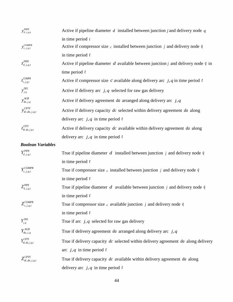
44
, , ,d j q t
PIPEy Active if pipeline diameter d installed between junction j and delivery node q
in time period t
, , ,
C
c j
R
q t
OMPy Active if compressor size c installed between junction j and delivery node q
in time period t
, , ,d j q t
PIPEz Active if pipeline diameter d available between junction j and delivery node q in
time period t
, , ,
C
c j
R
q t
OMPz Active if compressor size c available along delivery arc ,j q in time period t
,
DEL
j qy Active if delivery arc ,j q selected for raw gas delivery
, ,
AGR
da j qy Active if delivery agreement da arranged along delivery arc ,j q
, , , ,dc da j q
Y
t
CPTy Active if delivery capacity dc selected within delivery agreement da along
delivery arc ,j q in time period t
, , , ,dc da j q
Y
t
CPTz Active if delivery capacity dc available within delivery agreement da along
delivery arc ,j q in time period t
Boolean Variables
, , ,d j q t
PIPEY True if pipeline diameter d installed between junction j and delivery node q
in time period t
, , ,
C
c j
R
q t
OMPY True if compressor size c installed between junction j and delivery node q
in time period t
, , ,d j q t
PIPEZ True if pipeline diameter d available between junction j and delivery node q
in time period t
, , ,
C
c j
R
q t
OMPZ True if compressor size c available junction j and delivery node q
in time period t
,
DEL
j qY True if arc ,j q selected for raw gas delivery
, ,
AGR
da j qY True if delivery agreement da arranged along delivery arc ,j q
, , , ,dc da j q
Y
t
CPTY True if delivery capacity dc selected within delivery agreement da along delivery
arc ,j q in time period t
, , , ,dc da j q
Y
t
CPTZ True if delivery capacity dc available within delivery agreement da along
delivery arc ,j q in time period t

45
Continuous Variables
0
,p tF Flow rate produced gas at well pad p in time period t
, j, ,
0
qp tF Flow rate produced gas at well pad p intended for delivery arc ,j q
in time period t (disaggregated variable)
, ,
PJ
p j tF Gas flow rate from well pad p to junction j in time period t
ˆ, ,p p
P
t
PF Gas flow rate from well pad p to well pad p in time period t
ˆ,, j
J
j t
JF Gas flow rate from junction j to junction j in time period t
, ,
Q
j q t
JF Gas flow rate along delivery arc ,j q in time period t
, , ,
KJQ
k j q tF Gas flow rate component k along delivery arc . ,j q .in time period t
, ,
S
j q tF Slack gas flow rate along delivery arc ,j q in time period t
, ,
J
k j tXF Molar fraction gas component k at junction j in time period t
tDVE Development expenses (drilling, fracturing, completion) in time period t
tFPE Flow pipeline construction expenses in time period t
tGPE Gathering pipeline construction expenses in time period t
tDPE Delivery pipeline construction expenses in time period t
tCIE Compressor installation expenses in time period t
tCOE Compressor operating expenses in time period t
tPME Production and maintenance expenses in time period t
tFWE Fresh water acquisition expenses in time period t
tRRE Royalty expenses in time period t
tRDE Drilling rig downtime expenses in time period t
tRTE Drilling rig transition expenses in time period t
, ,r p tRTE Drilling rig transition expenses in time period t (auxiliary variable)
, ,r p tRTE Drilling rig transition expenses in time period t (auxiliary variable)
tSCE Well site construction expenses in time period t
tPRE Processing expenses in time period t
, ,j q tPRE Processing expenses along delivery arc ,j q in time period t
tREV Revenues from natural gas sales in time period t
, ,j q tREV Revenues from natural gas sales along arc ,j q in time period t
,p tNWD Number of wells that have been completed at well pad p in time period t

46
,p tNWP Number of wells producing shale gas at well pad p in time period t
, ,f p tFWS Fresh water supply from fresh water source f to well pad p in time period t
NPV Net present value of the shale gas development project
Parameters
dr Discount rate (annual or monthly depending on time discretization)
nd Number of days per time period
0
,p kx Molar fraction shale gas component k produced gas at well pad p
, ,k q tp Price of natural gas component k at delivery node q in time period t
D Well development cost coefficient
A
da Processing cost coefficient for delivery agreement da
P Pipeline construction cost coefficient
C Compressor installation cost coefficient
I Production cost coefficient
O Compressor operating cost coefficient
W Fresh water acquisition cost coefficient
R Rig transition cost coefficient
RD Rig downtime cost coefficient
S Site construction cost coefficient
D Well development cost exponent
P Pipeline construction cost exponent
C Compressor installation cost exponent
d Commercially available pipeline diameters
0
,j q Pre-installed pipeline capacity (diameter) along arc ,j q
0
,j j Pre-installed pipeline capacity (diameter) along arc ,j j
0
i, j Pre-installed pipeline capacity (diameter) along arc ,i j
0
i,i Pre-installed pipeline capacity (diameter) along arc ,i j
,j ql Pipeline segment length from junction j to delivery node q
ˆ,j jl Pipeline segment length from junction j to junction j
,p jl Pipeline segment length from well pad p to junction j
, ppl Pipeline segment length from well pad p to well pad p

47
,f pl Pipeline segment length from fresh water source f to well pad p
c Commercially available compressor sizes
0
,j q Pre-installed compression power along arc ,j q
prr Royalty rate at well pad p
S
p Site construction lead time well pad p
D
n
W Well development lead time for a total of n wells being developed
R
n
D Drilling lead time for a total of n wells being drilled
F
n
H Fracturing lead time for a total of n wells being fractured (and completed)
P Pipeline construction lead time
C Compressor installation lead time
,
A
dc da Agreement length for delivery capacity dc under delivery agreement da
,
x
p t
man Maximum number of wells permitted at well pad p in time period t
,tp Well productivity at well pad p for a well of age a t time periods
, , ,dc da j q Maximum delivery quantity under delivery capacity dc within delivery
agreement da along delivery arc ,j q
, , ,dc da j q Minimum delivery quantity under delivery capacity dc within delivery agreement
da along delivery arc ,j q
Pk Pipeline capacity coefficient
Ck Compressor capacity coefficient
pfwd Specific fresh water demand per well pad p
,f tfwa Fresh water availability at fresh water source f in time period t
, ,
max
j q tf Maximum molar shale gas flowrate along delivery arc ,j q in time period t
, ,
max
j q trev Maximum revenues along delivery arc ,j q in time period t
max
tcapex Capital expenditures limit
kh Heating value gas component k
min
, , ,dc da j qh Minimum heating value imposed for delivery capacity dc within delivery
agreement da along delivery arc ,j q
max
, , ,dc da j qh Maximum heating value imposed for delivery capacity dc within delivery
agreement da along delivery arc ,j q

48
, ,
PRE
da j qm Big-M parameter for processing expenses under delivery agreement da along
delivery arc ,j q
, ,da j
V
q
REm Big-M parameter for revenues under delivery agreement da along
delivery arc ,j q
, , ,dc da j qm Big-M parameter for minimum delivery quantity under delivery capacity dc
within delivery agreement da along delivery arc ,j q
, , ,dc da j qm Big-M parameter for maximum delivery quantity under delivery capacity dc
within delivery agreement da along delivery arc ,j q
, , ,
minh
dc da j qm Big-M parameter for minimum heating value specification under delivery
capacity dc within delivery agreement da along delivery arc ,j q
, , ,
maxh
dc da j qm Big-M parameter for maximum heating value specification under delivery
capacity dc within delivery agreement da along delivery arc ,j q
References
1. U.S. Energy Information Administration (EIA), 2014. Annual Energy Outlook 2014 with projections to 2040. U.S.
Department of Energy Information. Office of Integrated and International Energy Analysis. Available at:
www.eia.gov/forecasts/aeo/pdf/0383(2014).pdf [last accessed September 2015].
2. Goellner, J.F., 2012. Expanding the shale gas infrastructure. Chemical Engineering Progress 108 (8), 49-52.
3. Tobin, J., Shambaugh, P., Mastrangelo, E., 2006. Natural Gas Processing: The Crucial Link between Natural Gas Production
and Its Transportation to Market. Energy Information Administration, Office of Oil and Gas.
http://www.eia.gov/pub/oil_gas/natural_gas/feature_articles/2006/ngprocess/ngprocess.pdf [last accessed September 2015].
4. Iyer, R.R., Grossmann, I.E., Vasantharajan, S., Cullick, A.S., 1998. Optimal planning and scheduling of offshore oil field
infrastructure investment and operations. Industrial & Engineering Chemistry Research 37 (4), 1380-1397.
5. van den Heever, S.A., Grossmann, I.E., 2000. An iterative aggregation/disaggregation approach for the solution of a mixed-
integer nonlinear oilfield infrastructure planning model. Industrial & Engineering Chemistry Research 39 (6), 1955-1971.
6. van den Heever, S.A., Grossmann, I.E., Vasantharajan, S., Edwards, K., 2001. A Lagrangean decomposition heuristic for
the design and planning of offshore hydrocarbon field infastructures with complex economic objectives. Industrial &
Engineering Chemistry Research 40 (13), 2857-2875.
7. Goel, V., Grossmann, I.E., 2004. A stochastic programming approach to planning of offshore gas field developments under
uncertainty in reserves. Computers and Chemical Engineering 28 (8), 1409-1429.
8. Selot, A., Kuok, L.K., Robinson, M., Barton, P.I., 2008. A short-term operational planning model for natural gas production
systems. AIChE Journal 54 (2), 495-515.
9. Tavallali, M.S., Karimi, I.A., Teo. K.M., Baxendale, D., Ayatollahi, S., 2013. Optimal producer well placement and
production planning in an oil reservoir. Computers & Chemical Engineering 55, 109-125.
10. Knudsen, B.R., Foss, B., 2013. Shut-in based production optimization of shale-gas systems. Comptuers & Chemical
Engineering 58, 54-67.
11. Knudsen, B.R., Grossmann, I.E., Foss, B., Conn, A.R., 2014. Lagrangian relaxation based decomposition for well
scheduling in shale-gas systems. Computers & Chemical Engineering 63, 234-249.
12. Knudsen, B.R., Whitson, C.H., Foss, B., 2014. Shale-gas scheduling for natural-gas supply in electric power production.
Energy 78, 165-182.

49
13. Yang, L., Grossmann, I.E., Manno, J., 2014. Optimization models for shale gas water management. AIChE Journal 60 (10),
3490-3501.
14. Yang, L., Grossmann, I.E., Mauter, M.S., 2015. Investment optimization model for freshwater acquisition and wastewater
handling in shale gas production. AIChE Journal 61 (6), 1770-1782.
15. Cafaro, D.C., Grossmann, I.E., 2014. Strategic planning, design, and development of the shale gas supply chain network.
AIChE Journal 60. 2122-2142.
16. Gao, J., You, F., 2015. Shale gas supply chain design and operations toward better economic and life cycle environmental
performance: MINLP model and global optimization algorithm. ACS Sustainable Chem. Eng. 3, 1282-1291.
17. Grossmann, I.E., and Trespalacios, F., 2013. Systematic modeling of discrete-continuous optimization models through
generalized disjunctive programming. AIChE Journal 59 (9), 3276-3295.
18. Park, M., Park, S., Mele, F. D., Grossmann, I.E., 2006. Modeling of purchase and sales contracts in supply chain
optimization. Industrial & Engineering Chemistry Research 45 (14), 5013-5026.
19. Pan, I., 2013. Natural gas processing contracts and how they affect profits and valuation. Market Realist. Available at:
http://marketrealist.com/2013/01/natural-gas-processing-contracts-and-how-they-affect-profits-and-valuation/ [last accessed
September 2015].
20. Moore, F.T., 1959. Economies of scale: Some statistical evidence. The Quarterly Journal of Economics, 232-125.
21. Haldi, J., Whitcomb, D., 1967. Economies of scale in industrial plants. The Journal of Political Economy, 373-385.
22. Tribe, M.A., Alpine, R.L.W., 1986. Scale economies and the “0.6 rule”. Engineering Costs and Production Economics 10
(4), 271-278.
23. Dawson, M., Howard, P., Salkeld, M., 2012. Improved Productivity in the Development of Unconventional Gas. Technical
Study for Productivity Alberta. Available at: http://www.csur.com/images/news/2012/productivityalbertaquestionnaire.pdf
[last accessed September 2015].
24. Quesada, I., Grossmann, I.E., 1995. Global optimization of bilinear process networks with multicomponent flows.
Computers & Chemical Engineering 19 (12), 1219-1242.
25. Duran, M.A., Grossmann, I.E., 1986. An outer-approximation algorithm for a class of mixed-integer nonlinear programs.
Mathematical Programming 36 (3), 307-339.
26. Viswanathan, J., Grossmann, I.E., 1990. A combined penalty function and outer approximation method for MINLP
optimization. Computers & Chemical Engineering 14, 769-782.
27. Grossmann, I.E., and Lee, S., 2003. Generalized convex disjunctive programming: nonlinear convex hull relaxation.
Computational Optimization and Applications 26, 466-486.
28. Castro, P.M., and Grossmann, I.E., 2012. Generalized disjunctive programming as a systematic modeling framework to
derive scheduling formulations. Industrial & Engineering Chemistry Research 51, 5781-5792.
Appendix A: Pipeline Sizing
As outlined in section Model Formulation: Single Delivery Node Problem we size gathering lines based
on fluid velocity. As a rule of thumb operators strive to ensure that the fluid velocity in gas lines does not
exceed 20 m/s to minimize noise emissions and allow for corrosion inhibition. We rely on this design
specification for preliminary pipeline sizing purposes. The necessary pipeline diameter ,j q is calculated
using Eq. (105).
2
, , , , ,60 J
j q j q t
g
Q
l
Pk
T zF j q t
v p
(105)

50
In Eq. (105), T is the gas temperature in K, z is the gas compressibility factor ( 1z due to the ideal gas
assumption), gv is the maximum gas velocity set to 20 m/s, and lp is the line pressure MPa. For simplicity,
we define the pipeline coefficient Pk as seen in Eq. (105) and use it for pipeline sizing purposes in Eqs.
(12) and (15). For a given gas flow , ,
JQ
j q tF in 106 m3/day and an unknown pipeline diameter ,j q in inches
the pipeline coefficient is 0.0026716Pk .
We note that once the gathering system has been sized using the proposed approach we generally advise
to use standard gas flow equations such as the Weymouth or Panhandle equations to calculate the explicit
pressure drops along individual pipeline segments. If these are beyond tolerable specifications a larger
diameter pipeline may be selected. In our experience, however, the sizing procedure based on gas velocity
provides a sufficiently good estimate of the required pipeline size and, generally, the calculated pressure
drops are reasonably small due to the relatively low line pressure and short lengths of the pipeline
segments.
Appendix B: Compact Hull Reformulation
Disjunctions are usually reformulated using either a Big-M (BM) or a Hull Reformulation (HR)
formulation17. Given disjunction (12) its HR is as follows.
0
, , , , , , ,JQ DJQ
j q t d j q t
Dd
F j q tF
(106)
2
0 2
,, , , , , , 0 , , ,P DJQ PIPE
d j q t d dq j q tj z dk q tF j (107)
, ,
, , , , , , , , , , , , , 0 , , ,JQ LOW PIPE DJQ JQ UP PIPE
j q t d j q t d j q t j q t d j q tF z F F z d j q t (108)
0
, , , 1 , ,PIPE
d
d
j q tz j q t
(109)
Compared to its alternative – the Big-M formulation – the HR requires the introduction of the
disaggregated variables , , ,
DJQ
d j q tF , the corresponding constraints as seen in Eq. (106), as well as two
constraints for each disaggregated variable (to impose lower and upper bounds on these variables) as
captured by Eq. (108). Therefore, the HR generally requires more variables and constraints than the BM.
This increase in model size oftentimes adds to the computational effort of solving the respective problems.
At the same time Grossmann and Lee27 show that the continuous relaxation of the HR formulation is as
least as tight as and generally tighter than the BM when the discrete domain is relaxed.
In the particular case of disjunction (12), however, it is possible to derive a compact HR: if, for a given
,j q and t , we sum up the inequality constraint (107) over all 0d then we get:

51
0 0
20 2
, , ,, , , , , ,j q
P DJQ PIPE
d j q t d q
d
d t
d
jz qF tk j
(110)
Next, we can replace the summation of the disaggregated variables , , ,
DJQ
d j q tF on the left-hand side of Eq.
(110) with their initial definition in Eq. (106) as shown below.
0
20 2
, , , ,, , , ,P JQ PIPE
j q t d d jj q q t
d
k F z j q t
(111)
Since Eq. (111) no longer involves any disaggregated variables, we can now drop Eqs. (106) and (108)
from the reformulation of the disjunction and merely impose regular bounds on the flow variables. Hence,
the compact HR is as follows.
0
20 2
, , , , , , , ,P
j q t j q d d j
JQ
q t
PIPE
d
k jF z q t
(112)
0
, , , 1 ( , ) ,PIPE
d j q t
d
z j q t
(113)
As highlighted by Castro and Grossmann28, the noteworthy property of the compact HR is that it combines
the advantages of the HR and the BM without introducing their respective shortcomings.
Appendix C: Compressor Sizing
The size of a compressor is determined in terms of its maximum power requirement. For this purpose we
assume adiabatic compression and a fixed compression ratio, i.e., suction and discharge pressure
specifications jPd and jPs are fixed. Given these assumptions the power requirement ,
C
j q is linearly
proportional to the gas flow , ,
JQ
j q tF as seen below.
1
, , , , ,1
4.0426 qC
j q j q t
Q
j
z
J
Ck
TF j t
Pdq
Ps
(114)
In Eq. (114) above T is the gas temperature at suction conditions in K (typically 298.15T K ),
represents the heat capacity ratio (typically 1.26 ), stands for the compressor efficiency (we assume
0.9 ), and finally z is the gas compressibility factor which we set to 1z due to the ideal gas
assumption. For simplicity, we define the compression coefficient Ck as seen in Eq. (114) and use it for
compressor sizing purposes in Eqs. (20) and (23). For a given gas flow , ,
JQ
j q tF in 106 m3/day and unknown
compression power ,
C
j q in kW the compression coefficient is 0.0023813Ck .

52
Figures
Fig. 1: Cross section through a typical shale gas well (left) and a multi-well pad configuration (right)
Fig. 2: Production profiles in million cubic feet per year for shale gas wells in major U.S. shale plays,
Source: U.S. Energy Information Administration (EIA), Annual Energy Outlook 2012
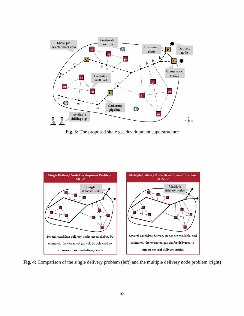
53
Fig. 3: The proposed shale gas development superstructure
Fig. 4: Comparison of the single delivery problem (left) and the multiple delivery node problem (right)

54
Fig. 5: Illustration of the three levels of strategic development constraints
Fig. 6: Illustration of equipment costs subject to economies of scale

55
Fig. 7: Multiple delivery node development problem indicating gas composition variations (grey shades)
Fig. 8: Illustration of gas flows at the intermediate splitting node.
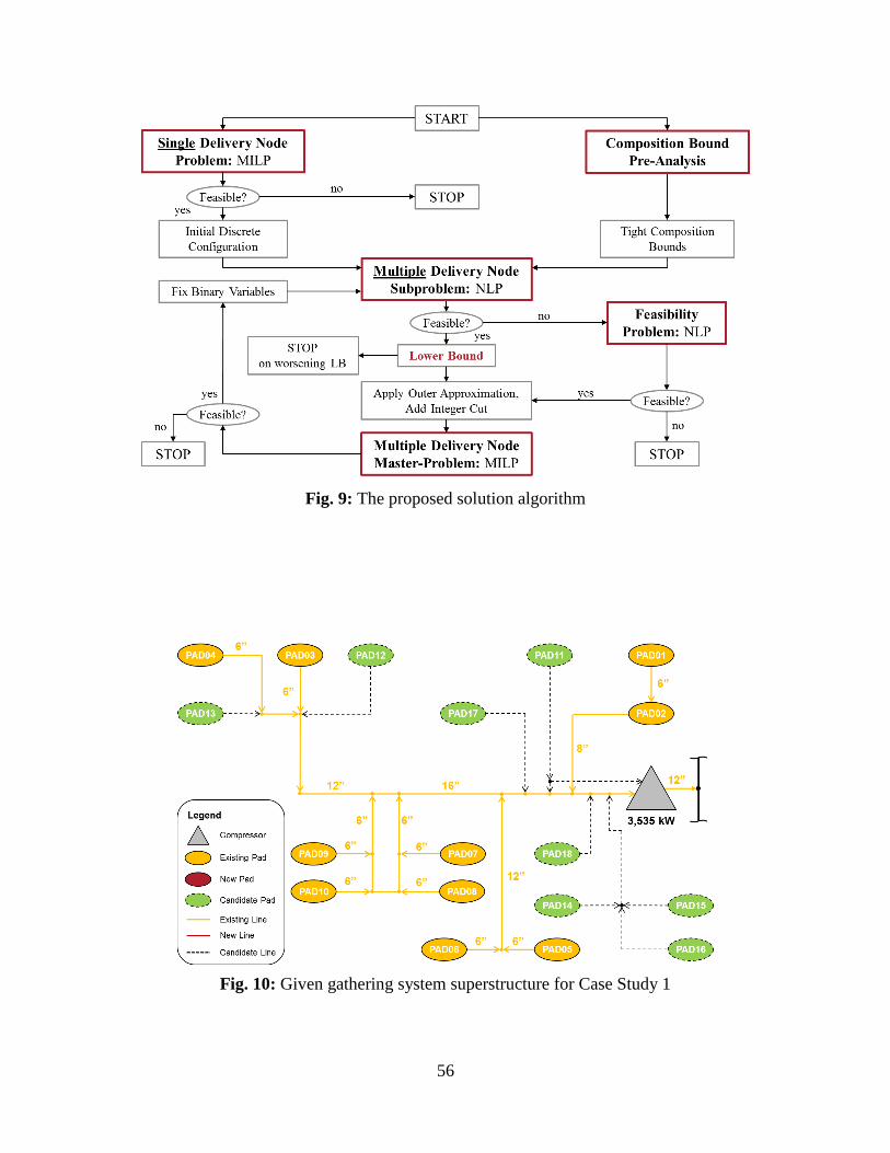
56
Fig. 9: The proposed solution algorithm
Fig. 10: Given gathering system superstructure for Case Study 1

57
Fig. 11: Optimal gathering system at the end of the planning horizon for Case Study 1
Fig. 12: Optimal development schedule (left) and historic development schedule (right)
for Case Study 1

58
Fig. 13: Optimal production profile (left) and historic production profile (right) for Case Study 1
Fig. 14: Given gathering system superstructure for Case Study 2

59
Fig. 15: Optimal gathering system for the SDN problem of Case Study 2
Fig. 16: Gas deliveries and selected processing agreements for the SDN problem of Case Study 2
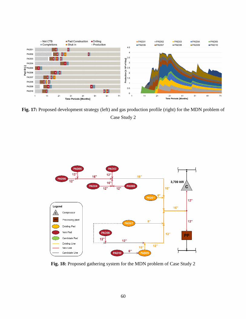
60
Fig. 17: Proposed development strategy (left) and gas production profile (right) for the MDN problem of
Case Study 2
Fig. 18: Proposed gathering system for the MDN problem of Case Study 2

61
Fig. 19: Gas deliveries and selected processing agreements for the MDN problem of Case Study 2
Fig. 20: Breakdown of development expenses (left) and projected revenues (right) for the MDN
problem of Case Study 2

62
Tables
Table 1: Available processing agreements and their conditions for Case Study 2