Accepted Manuscript

Multi-stage multi-product multi-period production planning with sequence-de-pendent setups in closed-loop supply chain

S. Torkaman, S.M.T Fatemi Ghomi, B. Karimi

PII: S0360-8352(17)30457-6DOI: https://doi.org/10.1016/j.cie.2017.09.040Reference: CAIE 4926

To appear in: Computers & Industrial Engineering

Received Date: 27 March 2016Revised Date: 12 March 2017Accepted Date: 23 September 2017

Please cite this article as: Torkaman, S., Fatemi Ghomi, S.M.T, Karimi, B., Multi-stage multi-product multi-periodproduction planning with sequence-dependent setups in closed-loop supply chain, Computers & IndustrialEngineering (2017), doi: https://doi.org/10.1016/j.cie.2017.09.040

This is a PDF file of an unedited manuscript that has been accepted for publication. As a service to our customerswe are providing this early version of the manuscript. The manuscript will undergo copyediting, typesetting, andreview of the resulting proof before it is published in its final form. Please note that during the production processerrors may be discovered which could affect the content, and all legal disclaimers that apply to the journal pertain.

1

Multi-stage multi-product multi-period production planning with sequence-

dependent setups in closed-loop supply chain

S.Torkaman a,b

, S.M.T Fatemi Ghomi a,c*

, B.Karimi a,d

a Department of Industrial Engineering, Amirkabir University of Technology, 424 Hafez

Avenue,1591634311 Tehran, Iran

b E-mail address: s.torkaman@aut.ac.ir

c Corresponding author. Tel.: (+9821) 64545381, Fax: (+9821) 66954569, E-mail address:

fatemi@aut.ac.ir

d Tel.: (+9821) 64545374, E-mail address: b.karimi@aut.ac.ir

2

Multi-stage multi-product multi-period production planning with

sequence-dependent setups in closed-loop supply chain

Abstract

This paper studies multi-stage multi-product multi-period capacitated production

planning problem with sequence dependent setups in closed-loop supply chain. In this

problem, manufacturing and remanufacturing of each product is regarded consequently,

and in addition to the setup for changing products, a setup while changing the processes

is needed. To formulate the problem, a mixed-integer programming (MIP) model is

presented. Four MIP-based heuristic named non-permutation and permutation

heuristics, using rolling horizon are utilized to solve this model. Moreover, a simulated

annealing algorithm using a heuristic to provide initial solution is developed to solve the

problem. To calibrate the parameters of the proposed simulated annealing algorithm,

Taguchi method is applied. The numerical results indicate the efficiency of the proposed

meta-heuristic algorithm against MIP-based heuristic algorithms.

Keywords Production planning, Closed-loop supply chain, Sequence dependent

setup, Rolling horizon, Simulated Annealing algorithm, Flow shop.

1. Introduction

The management of return flows has been increasingly paid attention by researchers

during last two decades. Contrary to traditional supply chain where the products flow

from manufacturers to customers, in closed-loop supply chain, the manufacturers often

collect the used products from the customers and reprocess them for a higher profit or

reduce the negative environmental effects.

In published literature in the field of closed-loop supply chain, numerous studies

have been made and a large number of models have been developed. Stindt and

Sahamie (2014) classified the quantitative studies of closed-loop supply chain in four

groups of network design, production planning, product returns management, and

forecasting. In closed loop supply chain there are different options for recovery such as

reuse, repair, remanufacturing, refurbishing, retrieval and recycling; in which

remanufacturing that transforms the defective products into an as-good-as new

condition is attractive in terms of environmental concerns, legislation and economics

(Stindt & Sahamie, 2014). Ilgin and Gupta (2010) categorized the studies in the field of

remanufacturing into six groups of forecasting, production planning and scheduling,

capacity planning, inventory management, and uncertainty effect.

Production planning in hybrid systems which includes manufacturing and

remanufacturing is an important issue in closed-loop supply chain, the purpose of which

is the optimum usage of production resources to produce the products according to the

demand in the planning horizon. In these problems, remanufacturing is used as well as

manufacturing to satisfy demands.

Production planning has been paid attention by researchers since early twentieth

century. It was first studied by Wagner and Whitin (1958); they solved a single-stage,

single-product, multi-period uncapacitated production planning using a forward

dynamic programming. Research in the field of production planning is vast and contains

3

numerous topics; one of the most complex of them is lot sizing. Bahl et al. (1987)

classified the lot sizing problems into four categories according to the number of levels

and resource capacity. Karimi et al. (2003) classified the lot sizing problems into the

capacitated lot sizing problem (CLSP), the economic lot scheduling problem (ELSP),

the discrete lot sizing and scheduling problem (DLSP), the continuous setup lot sizing

problem (CSLP), the proportional lot sizing and scheduling problem (PLSP) and the

general lot sizing and scheduling problem (GLSP), all of which are NP-hard in case of

capacity constraint. Production planning or specifically lot sizing with remanufacturing

is the focus of the current study.

Lot sizing in hybrid systems including manufacturing and remanufacturing is

considered in many studies of closed-loop supply chain. First, Richter and Weber

(2001) developed reverse Wagner-Whitin model for hybrid lot sizing problem, and

proved that in the case of constant cost and demand, the optimal policy is starting

remanufacturing before exchanging to manufacturing process. Yang et al. (2005)

considered an uncapacitated problem with concave cost functions, and cited that even in

the case of constant costs, the problem would be NP-hard. This problem is modelled as

a network flow type formulation, and a polynomial time heuristic has been utilized to

solve it. Teunter et al.(2006) considered two schemes for setup cost: a common setup

cost for manufacturing and remanufacturing for single production line; or different

setup cost for dedicated lines. In case of common production line, an exact polynomial

time dynamic programming algorithm is presented. For both cases, heuristic methods as

extensions of Silver-Meal method, Least Unit Cost method, and Part Period Balancing

method have been proposed. Li et al. (2006) studied a multi-product problem with

demand substitution, in which a higher quality product can satisfy the demand of a

lower quality one, in case of large amounts of returned products, a dynamic

programming method has been proposed to obtain a near optimal solution. Pan et al.

(2009) investigated the problem with disposal of returned products. This problem has

been analysed under different scenarios and solved using dynamic programming

algorithm. Pineyro and Viera (2010) and Z.-H.Zhang et al. (2012) studied the problem

with different demands for new and remanufactured products. Zhang et al. (2011)

considered the startup cost in the first period among periods with positive production,

Genetic algorithm is developed to solve the problem. Corominas et al. (2012) focused

on overtime, lost demands and the variety of returned products. The proportion of

returned products is a nonlinear function of their paid price. To solve the problem, the

objective function and constraints have been linearized via piecewise functions. Chen

and Abrishami (2014) assumed separate demand for new and remanufactured products

and developed a Lagrangian decomposition based method to solve the problem. Li et al.

(2014) developed a robust tabu search algorithm to solve the problem and evaluated it

using 6480 benchmark instances. Baki et al. (2014) proposed a new MIP formulation

for the problem with better bound when integrality constraints are relaxed. They

developed a dynamic programming based heuristic with some improvement schemes to

solve the problem. Lee et al. (2015) studied a capacity and lot sizing problem and

developed two linear programming relaxation based heuristics to solve it. Sifaleras and

Konstantaras (2015) proposed general variable neighbourhood search (GVNS)

algorithm to solve the problem. Parsopoulos et al. ( 2015) introduced some modification

in the problem formulation and developed a modified differential evolution (DE)

algorithm to solve the problem. Jing et al. (2016) considered the problem with

backorder and multiple factories to produce new products, remanufactured products, or

both. They presented three models to consider different cases and proposed an approach

4

based on self-adaptive genetic algorithm with population division (SAGA-PD) to solve

the problem.

The existing uncertainties in closed-loop supply chain which are due to the

amount and quality of returned products, the reprocessing time, effective yield and

customer demand, incur the planning complexity (Stindt & Sahamie, 2014). Some of

these uncertainties especially uncertain quantity and quality of returned products are

considered in lot sizing with remanufacturing. Li et al. (2013) considered the stochastic

and price-sensitive amount and the uncertain quality of returned products. Kenne et al.

(2012) regarded two machines for manufacturing and remanufacturing with stochastic

failures and repairs. Mukhopadhyay and Ma (2009) considered the uncertainty of

demand and returned products’ quality. Shi et al. (2010), Wei et al. (2011) , Naeem et

al. (2013) and Hilger et al. (2015) considered the uncertainty of the amount of returned

products and demand. Dong et al. (2011) focused on uncertainty of returned products’

quality, the time of returning, and reprocessing time. They regarded inspection,

recovery, and assembly operations for remanufacturing. Macedo et al. (2016)

considered the uncertain demand, return rate and setup cost due to quality of returned

products. They used a two-stage stochastic programming model to deal with the

uncertainties.

One of the most common complexities in lot sizing problems is setup time, which is

usually associated with changing tools and cleaning machines. Sequence-dependent

setup time is one of the most complex setups where the setup time of current product

depends on the previous scheduled product. Sequence-dependent setup time in lot sizing

problem for single machine has been considered by many researchers; Gupta and

Magnusson (2005) developed a heuristic method to solve the lot sizing problem with

sequence dependent setups and proposed a procedure to achieve a lower bound for the

problem. Almada-Lobo et al. (2007) proposed two linear mixed-integer programming

(MIP) models for CLSP with sequence dependent setup time and cost, and developed a

five-step heuristic approach to solve the problem. Kovács et al. (2009) presented a new

approach to model the CLSP with sequence dependent setup time; in which they

introduced a binary variable to indicate whether a product is produced or not, and

consider prespecified efficient sequences. Almada-Lobo and James (2010) proposed a

neighbourhood search algorithm to solve the CLSP with sequence-dependent setup

time. Menezes et al. (2011) studied the problem with non-triangular setups and solved

some examples using CPLEX software. James and Almada-Lobo (2011) considered the

CLSP with sequence-dependent setup in systems with parallel machines. They proposed

an iterative neighbourhood search heuristic based on MIP formulation to solve the

problem.

The multi-stage production system with complex setups in lot sizing problem has

been studied in recent years. Mohammadi et al. (2010) proposed a multi-product, multi-

period lot sizing problem with sequence dependent setups and setup carry-over in a flow

shop. To formulate the problem, for each machine and each period, N (the number of

products) setups are considered, and artificial setups from one product to the same one

are permitted. They used a rolling-horizon and fix-and-relax heuristics to solve the

problem. Mohammadi et al. (2011) proposed a genetic algorithm to solve the lot-sizing

problem with sequence dependent setups in permutation flow shop. Ramezanian et al.

(2013) considered a flow shop system and modelled the problem more efficiently than

Mohammadi et al. (2010) and Mohammadi et al. (2011) using starting and completion

time of production. They solved the problem using rolling horizon framework in

permutation cases. Mohammadi (2010) and Mohammadi and Jafari (2011) considered

the problem in flexible flow shops and developed MIP-based iterative approaches to

5

solve the problem. Ramezanian et al. (2013) considered the problem with uncertain

processing times and demand and developed a hybrid simulated annealing (SA)

algorithm to solve it. Ramezanian et al. (2016) studied the problem in flexible flow

shop environment and used rolling horizon heuristic and particle swarm optimization

algorithm (PSO) to solve the problem. Urrutia et al. (2014) and Wolosewicz et al.

(2015) considered the job shop systems and assumed that schedule of processing

products are predetermined. Although the sequence dependent setups have been

considered in many lot sizing studies, none of them consider remanufacturing.

Considering the real characteristics such as multi-stage production system and

complex setups like sequence dependent setup and setup carry-over makes the lot sizing

problem more complex in terms of modelling and solving, but multi-stage production

system with complex setups is not considered in the previous studies of closed loop

supply chain. Therefore, the motivation for this study is developing a more

comprehensive model considering the multi stage system with complex setups including

sequence dependent setup and setup carry-over, and remanufacturing in order to

implement in complicated industries such as auto car factory.

To the best knowledge of our literature review, the conducted studies of lot sizing in

closed loop supply chain considered a single stage production system with simple

setups. Therefore, the main contribution of the current study is considering a multi-stage

lot sizing problem with sequence dependent setups and setup carry-over in closed loop

supply chain, in which it is required to determine the scheduling and sequencing of

processes beside products. The preservation of setup over idle period is also considered

in this study. A mixed integer programming is introduced to formulate the problem

and the problem is solved by rolling horizon heuristic methods and a SA algorithm.

Moreover, Taguchi method is applied to calibrate the SA parameters.

The paper is organized as follows. Section 2 gives the problem assumptions and the

MIP model to formulate the problem. Heuristic methods, SA and Taguchi methods are

introduced in section 3. Section 4 includes computational results; and eventually,

section 5 is devoted to the conclusions and suggestions for further researches.

2. Problem assumptions and formulation

2.1. Assumptions

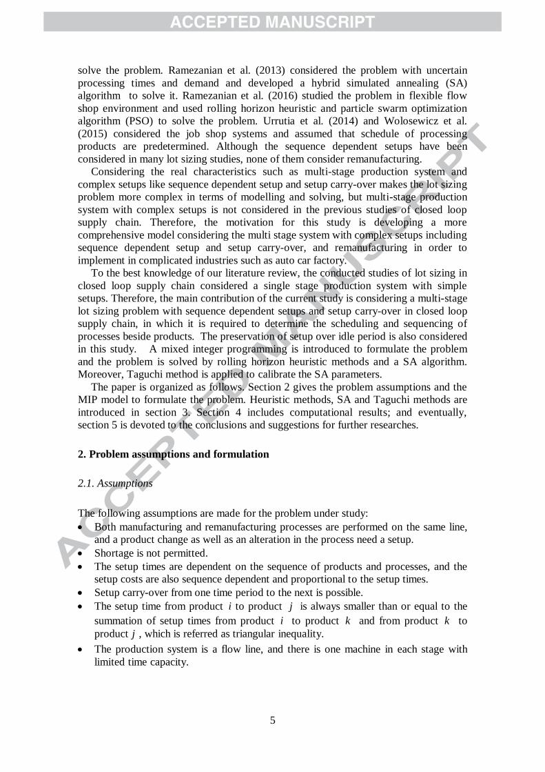
The following assumptions are made for the problem under study:

Both manufacturing and remanufacturing processes are performed on the same line,

and a product change as well as an alteration in the process need a setup.

Shortage is not permitted.

The setup times are dependent on the sequence of products and processes, and the

setup costs are also sequence dependent and proportional to the setup times.

Setup carry-over from one time period to the next is possible.

The setup time from product i to product j is always smaller than or equal to the

summation of setup times from product i to product k and from product k to

product j , which is referred as triangular inequality.

The production system is a flow line, and there is one machine in each stage with

limited time capacity.

6

Processing at a stage could only be started if a sufficient amount of the required

components from the previous stage are available; which is called vertical

interaction.

In the beginning of planning horizon, machines are set up for a specific process of a

specific product.

The final products obtained from both manufacturing and remanufacturing

processes have similar qualities and are named service products, which are utilized

to satisfy demands.

The inventories of intermediate products from manufacturing and remanufacturing

are stored separately.

The returned products are available in the beginning of each period.

Returned products have different quality levels. The remanufacturing time and cost

depend on these quality levels.

Defective products of manufacturing are used for remanufacturing, as well as

returned products.

The initial inventories are all zero.

When machine setup for product j finishes, the machine is ready to perform the

first process of product j .

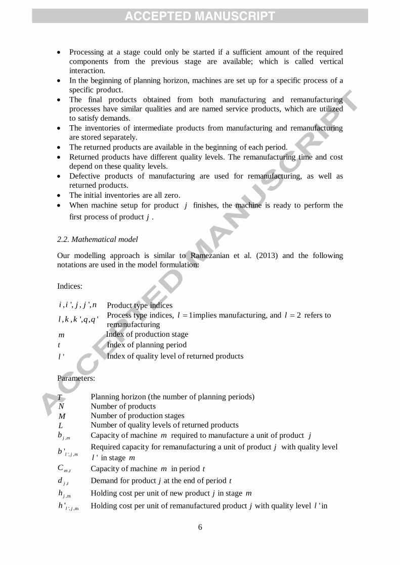
2.2. Mathematical model

Our modelling approach is similar to Ramezanian et al. (2013) and the following

notations are used in the model formulation:

Indices:

Product type indices , ', , ',i i j j n

Process type indices, 1l implies manufacturing, and 2l refers to

remanufacturing , , ', , 'l k k q q

I Index of production stage m

Index of planning period t

Index of quality level of returned products 'l

Parameters:

Planning horizon (the number of planning periods) T Number of products N

Number of production stages M Number of quality levels of returned products L

Capacity of machine m required to manufacture a unit of product j ,j mb

Required capacity for remanufacturing a unit of product j with quality level

'l in stage m ', ,'l j mb

Capacity of machine m in period t ,m tC

Demand for product j at the end of period t ,j td

Holding cost per unit of new product j in stage m ,mjh

Holding cost per unit of remanufactured product j with quality level 'l in ', ,m'l jh

7

stage m

Holding cost per unit of service product j jhs

Holding cost per unit of returned product. j .with quality level 'l ',l jhr

Manufacturing cost per unit of product j in stage m and period t ,m,tjp

Remanufacturing cost per unit of product j with quality level 'l in stage m

and period t ', ,m,t'l jp

Sequence-dependent setup time when switching from product i to product j

in stage m . If i j , , , 0i j mS ; Otherwise,

, , 0i j mS , ,i j mS

Sequence-dependent setup cost when switching from product i to product j

in stage m . If i j , , , 0i j mW ; Otherwise,

, , 0i j mW , ,i j mW

A fraction of new product j which is defective and retains quality level 'l ',l jr

The amount of returned product j with quality level 'l in period t ', ,l j tu

Sequence-dependent setup time when switching from process l of product j

to process k in stage m . If l k , , , , 0l k j mr ;Otherwise,

, , , 0l k j mr , , ,l k j mr

Sequence-dependent setup cost when switching from process l of product j

to process k in stage m . If l k , , , , 0l k j mc ; Otherwise,

, , , 0l k j mc , , ,l k j mc

Machines are set up to produce product 0j in the beginning of planning

horizon 0j

Machines are set up to perform process 0l in the beginning of planning

horizon 0l

A large real number bigM

Continuous decision variables:

Inventory of new product j in stage m at the end of period t , ,j m tI

Inventory of remanufactured product j with quality level 'l in stage m at the

end of period t ', , ,'l j m tI

Inventory of service product j at the end of period t ,j tIs

Inventory of returned product j with quality level 'l at the end of period t ', ,l j tIr

Manufacturing amount of product j in stage m and period t , ,j m tx

Remanufacturing amount of product j with quality level 'l in stage m and

period t ', , ,'l j m tx

Manufacturing starting time for product j on machine m in period t , ,j m tso

Manufacturing completion time for product j on machine m in periodt , ,j m tco

Remanufacturing starting time for product j on machine m in period t , ,' j m tso

Remanufacturing completion time for product j on machine m in period t , ,' j m tco

0, if exactly one product is produced in stage m and period t ; non-negative

value, otherwise. ,m t

0, if exactly one process of product j is performed in stage m and periodt ;

non-negative value, otherwise. , ,' j m t

8

Binary decision variables:

1, if the setup changes from product i to product j in stage m and period t ;

0, otherwise. , , ,i j m ty

1, if the setup changes from process l to process k of product j in stage m

and period t ; 0, otherwise. , , , ,l k j m tz

1, if process l of the product j is performed in stage m and period t ; 0,

otherwise. , , ,l j m tv

1, if product i is processed last in period 1t and product j is processed

first in period t and stage m ; 0, otherwise. , , ,'i j m ty

1, if setup for product j is carried from period 1t to period t in stage m ,

and process l is the last process of product j in period 1t , and process k

is the first process of product j in period t and stage m ; 0, otherwise.

, , , ,'l k j m tz

1, if manufacturing or remanufacturing of product j is performed in stage

m and period t ; 0, otherwise. ,m,j tT

1, if at least one product is produced in stage m and period t ; 0, otherwise. ,m tw

1, if product j is the first product in stage m and periodt ; 0, otherwise. , ,j m t

1, if product j is the last product in stage m and periodt ; 0, otherwise. , ,j m t

1, if process l is the first process of product j in stage m and period t ; 0,

otherwise. , , ,'l j m t

1, if process l is the last process of product j in stage m and period t ; 0,

otherwise. , , ,'l j m t

It should be mentioned that although, , ,'i j m ty ,

, , , ,'l k j m tz , ,m,j tT and

,m tw are defined as

binary variables, they can be relaxed as , , ,0 ' 1i j m ty ,

, , , ,0 ' 1l k j m tz ,,m,0 1j tT

and ,0 1m tw during solving. It means that, even if they are considered as continuous

variables, the value of them would be either one or zero due to structure of the presented

MIP model. Therefore, it is not necessary to restrict them to be integer.

With respect to the above-mentioned assumptions and notations, the MIP model would

be as follows:

Objective function:

(1)

1

, , , , ', , , ', , , , , ,

1 1 1 ' 1 1 1 1 1 1 1

1

', , ', , , ', , ', , , ,

' 1 1 1 1 ' 1 1 1 1

. ' . ' .

h' . ' . .

N M T L N M T N M T

j m t j m t l j m t l j m t j m j m t

j m t l j m t j m t

L N M T L N T T

l j m l j m t l j t l j t j t j t

l j m t l j t j t

Min p x p x h I

I hr Ir hs Is

1

2 2

, , , , , , , , , , , , , , , , , , ,

1 1 1 1 1 1 1 1 1

.( ' ) .( ' )

N

N N M T N M T

i j m i j m t i j m t l k j m l k j m t l k j m t

i j m t l k j m t

w y y c z z

9

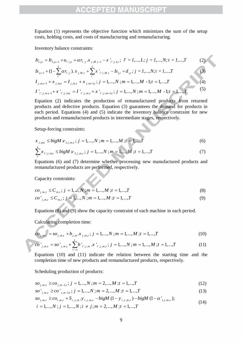
Equation (1) represents the objective function which minimizes the sum of the setup

costs, holding costs, and costs of manufacturing and remanufacturing.

Inventory balance constraints:

(2) l', j,t l', j,t 1 ', j,t ', , , 1 ', ,1,. ' ; l l j j M t l j tIr Ir u r x x l' = 1,...,L; j = 1,...,N; t = 1,...,T

(3) j,t 1 ', , , ' , , j,t j,t

' '

(1 ). 'L L

l j j M t l j M t

l l

Is r x x Is d ; j = 1,...,N;t = 1,...,T

(4) , , -1 ,m, , , ,m 1, ; 1,..., ; 1,..., -1; 1,...,j m t j t j m t j tI x I x j N m M t T

(5)

', , , -1 ', ,m, ', , , ', ,m 1,' ' ' ' ; 1,..., ; 1,..., -1; 1,...,l j m t l j t l j m t l j tI x I x j N m M t T

Equation (2) indicates the production of remanufactured products from returned

products and defective products. Equation (3) guarantees the demand for products in

each period. Equations (4) and (5) indicate the inventory balance constraint for new

products and remanufactured products in intermediate stages, respectively.

Setup-forcing constraints:

(6) ,m, 1, , ,. ; 1,..., ; 1,..., ; 1,...,j t j m tx bigM v j N m M t T

(7) ', ,m, 2, , ,

'

. ; 1,..., ; 1,..., ; 1,...,L

l j t j m t

l

x bigM v j N m M t T

Equations (6) and (7) determine whether processing new manufactured products and

remanufactured products are performed, respectively.

Capacity constraints:

(8) , , , ; 1,..., ; 1,..., ; 1,...,j m t m tco C j N m M t T

(9) , , ,' ; 1,..., ; 1,..., ; 1,...,j m t m tco C j N m M t T

Equations (8) and (9) show the capacity constraint of each machine in each period.

Calculating completion time:

(10) , , , , , , ,. ; 1,..., ; 1,..., ; 1,...,j m t j m t j m j m tco so b x j N m M t T

(11) , , , , ', , ', , ,

' 1

' ' ' . ' ; 1,..., ; 1,..., ; 1,...,L

j m t j m t l j m l j m t

l

co so b x j N m M t T

Equations (10) and (11) indicate the relation between the starting time and the

completion time of new products and remanufactured products, respectively.

Scheduling production of products:

(12) , , , 1, ; 1,..., ; 2,..., ; 1,...,j m t j m tso co j N m M t T

(13) , , , 1,' ' ; 1,..., ; 2,..., ; 1,...,j m t j m tso co j N m M t T

(14) , , , , , , , , , , , , 1, , ,. (1 ) (1 ' );

1,..., ; 1,..., ; ; 2,..., ; 1,...,

j m t i m t i j m i j m t i j m t j m tso co S y bigM y bigM

i N j N i j m M t T

10

(15) , , , , , , , , , , , , 1, , ,' . (1 ) (1 ' );

1,..., ; 1,..., ; ; 2,..., ; 1,...,

j m t i m t i j m i j m t i j m t j m tso co S y bigM y bigM

i N j N i j m M t T

(16) , , , , , , , , , , , , 2, , ,' . (1 ) (1 ' );

1,..., ; 1,..., ; ; 2,..., ; 1,...,

j m t i m t i j m i j m t i j m t j m tso co S y bigM y bigM

i N j N i j m M t T

(17) , , , , , , , , , , , , 2, , ,' ' . (1 ) (1 ' );

1,..., ; 1,..., ; ; 2,..., ; 1,...,

j m t i m t i j m i j m t i j m t j m tso co S y bigM y bigM

i N j N i j m M t T

(18) , , , , 2,1, , , 2,1, , 2,1, , ,' (1 ) . ; 1,..., ; 1,..., ; 1,...,j m t j m t j m t j m j m tso co bigM z r z j N m M t T

(19) , , , , 1,2, , , 1,2, , 1,2, , ,' (1 ) . ; 1,..., ; 1,..., ; 1,...,j m t j m t j m t j m j m tso co bigM z r z j N m M t T

Equations (12) and (13) represent that the processing of product j in stage m could

begin if only the processing of this product has finished in stage 1m . Equations (14)-

(17) represent that if processing of product j is planned after product i on machine m ,

the first process of product j could only begin if the processing of product i has

finished on this machine, and the setup for product j has been performed. Equations

(18) and (19) indicate that the last process of product j on machine m , could only

begin if the first process of product j has been completed on this machine, and setup for

the last process has been performed.

Sequencing the products:

(20) , , , , ,

1 1,i j 1

1; 1,..., ; 1,...,N N N

i j m t j m t

i j j

y T m M t T

(21) 2 2 2

,k, , , , , ,

1 1, 1

1; 1,..., ; 1,..., ; 1,...,l j m t l j m t

l k l k l

z v j N m M t T

(22)

2

, , , , ,

1

2. ; 1,..., ; 1,..., ; 1,...,l j m t j m t

l

v T j N m M t T

(23) , , , , ,

1,i j

; 1,..., ; 1,..., ; 1,...,N

i j m t j m t

i

y T j N m M t T

(24) , , , , ,

1,i j

; 1,..., ; 1,..., ; 1,...,N

j i m t j m t

i

y T j N m M t T

Equations (20) and (21) indicate that changing products and processes require setup.

Equation (22) implies that if at least one process of product j is performed, , ,j m tT would

be 1. Equations (23) and (24) indicate that product j can only be within a sequence of

products if it is produced in stage m and period t .

Set up carry-over of products:

(25) , , ,

1

. ; 1,..., ; 1,...,N

j m t m t

j

T bigM w m M t T

11

(26) , , ,

1

1 ( 1). ; 1,..., ; 1,...,N

j m t m t

j

T N m M t T

(27) , , ,

1

; 1,..., ; 1,...,N

j m t m t

j

w m M t T

(28) , , ,

1

; 1,..., ; 1,...,N

j m t m t

j

w m M t T

(29) , , , , , , ,

1

; 1,..., N; 1,..., ; 1,...,N

j m t j m t i j m t

i

T y j m M t T

(30) , , , , , , ,

1

; 1,..., ; 1,..., ; 1,...,N

j m t j m t j i m t

i

T y j N m M t T

(31) , , , , ,2 ; 1,..., ; 1,..., ; 1,...,j m t j m t m t j N m M t T

(32) 0 , j, ,1

1

' 1; 1,...,N

j m

j

y m M

(33) i, , , , ,

1

' ; 1,..., ; 1,..., ; 1,...,N

j m t j m t

i

y j N m M t T

(34) i, , , , , 1

1

' ; 1,..., ; 1,..., ; 1,...,N

j m t i m t

j

y i N m M t T

(35) i, j, ,

1 1

' 1; 1,..., ; 1,...,N N

m t

i j

y m M t T

(36) ', , , 1 , , , 1 , , , , ', , 1

' 1 1, 1 ' 1, '

' ' ; 1,..., ; 1,..., ; 2,...,N N N N

j j m t i j m t j n m t j i m t

j i i j n i i j

y y y y j N m M t T

Equation (25) states that in case of producing at least one product, ,m tw should be one.

According to Equations (27) and (28), even if ,m tw is relaxed as ,0 1m tw , it would

be either one or zero; since ,m tw equals the summation of several binary variables, it

retains an integer value, on the other hand, since it is defined as ,0 1m tw , it cannot

be of a value more than 1. Equation (26) states that if more than one product is

produced within a period, ,m t should be positive. Equations (27) and (28) indicate that

if production is performed in one stage and one period, only one product can be the first

or last produced product. According to Equations (29) and (30), if a product is not the

first or last product, the corresponding or would be zero, respectively. Equation

(31) states that if only one product is produced in a period, would be zero. Equations

(32) indicate that machines are setup in the beginning of the planning horizon for

product 0j . Regarding Equations (33) and (34), if product j is the first product in stage

m and period t , and product i is the last product in stage m and period 1t , the

, , ,'i j m ty variable would equal 1. Equation (35) claims that the setup for exactly one

product is carried over from period 1t to period t . Equation (36) guarantees the

preservation of setup related to products over idle period.

12

Set up carry-over of processes:

(37) 0 0 0 0

2

, , , ,1 , , ,1

1

' ' ; 1,...,l l j m j j m

l

z y m M

(38)

2

, , , , ,

1

' ; 1,..., N; 1,..., ; 1,...,l j m t j m t

l

T j m M t T

(39)

2

, , , , ,

1

' ; 1,..., N; 1,..., ; 1,...,l j m t j m t

l

T j m M t T

(40)

2

, , , , ,

1

1 ' ; 1,..., N; 1,..., ; 1,...,l j m t j m t

l

v j m M t T

(41) , , , , , , , ,' ' 2 ' ; 1,2; 1,..., ; 1,..., ; 1,...,l j m t l j m t j m t l j N m M t T

(42) , , , , , , , , , ,' ; 1,2; 1,2; ; 1,..., ; 1,..., ; 1,...,l j m t l j m t k l j m tv z l k l k j N m M t T

(43) , , , , , , , , , ,' ; 1,2; 1,2; ; 1,..., ; 1,..., ; 1,...,l j m t l j m t l k j m tv z l k l k j N m M t T

(44)

2

, , , , , , , , , ,

1

' .(1 ' ) ' ; 1,2; 1,..., ; 1,..., ; 1,...,k l j m t j j m t l j m t

k

z bigM y l j N m M t T

(45)

2

, , , , , , , , , , 1

1

' .(1 ' ) ' ; 1,2; 1,..., ; 1,..., ; 1,...,k l j m t j j m t k j m t

l

z bigM y k j N m M t T

(46)

, , , , , , , l,1, , ,1, , , 1, , ,

1 1

. ' . ' (1 ' );

1,..., ; 1,..., ; 1,...,

N L

j m t i j m i j m t j m l j m t j m t

i l

so S y r z bigM

j N m M t T

(47) , , , , , , , ,2, , ,2, , , 2, , ,

1 1

' . ' . ' (1 ' );

1,..., ; 1,..., ; 1,...,

N L

j m t i j m i j m t l j m l j m t j m t

i l

so S y r z bigM

j N m M t T

(48)

2 2

k,l, , , j, j, ,

1 1

' ' ; 1,..., ; 1,..., ; 1,...,j m t m t

l k

z y j N m M t T

(49)

2 2

, , , , 1 , , , 1 , , , , 1 , ', , , , , , , ', , , 1

1 ' 1

' (1 ' ) ' (1 ' ) ;

1,2; 1,2; ' 1,2; ; '; 1,..., ; 1,..., ; 2,...,

k l j m t j j m t q l j m t l q j m t j j m t l k j m t

k q

z bigM y z z bigM y z

l q k q l l k j N m M t T

Equations (37) indicate that machines are setup in the beginning of the planning horizon

for process 0l of product 0j . Similarly to ,m tw , if , ,j m tT is relaxed as continuous variable

between zero and one, it retains the value zero or one, according to Equations (38) and

(39). Additionally, according to these equations, only one of the processes of a

produced product in one period and in a specific stage could be the first or last process.

Equation (40) states that if both processes of manufacturing and remanufacturing are

performed in one period, , ,' j m t should be positive. Equation (41) indicates that if

exactly one of the processes is performed, ' would be zero. Equations (42) and (43)

show that if a process is not the first or last process of produced product j , the

13

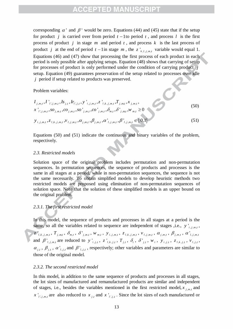
corresponding ' and ' would be zero. Equations (44) and (45) state that if the setup

for product j is carried over from period 1t to period t , and process l is the first

process of product j in stage m and period t , and process k is the last process of

product j at the end of period 1t in stage m , the , , , ,'k l j m tz variable would equal 1.

Equations (46) and (47) show that processing the first process of each product in each

period is only possible after applying setups. Equation (48) shows that carrying of setup

for processes of product is only performed under the condition of carrying product j

setup. Equation (49) guarantees preservation of the setup related to processes over idle

j period if setup related to products was preserved.

Problem variables:

(50) , , ', , , , ', , , , , , , , , ,m, , ,

', , , , , , , , , , , , ,m, ,

, ' , , , ' , ' , , ,

' , , , ' , ' , , ' , 0

j m t l j m t j t l j t i j m t l k j m t j t j m t

l j m t j m t j m t j m t j m t m t j t m t

I I Is Ir y z T x

x so co so co w

(51) , , , , , , , , , , , , , , , , , , , ,, , , , , ' , ' 0,1i j m t l k j m t l j m t j m t j m t l j m t l j m ty z v

Equations (50) and (51) indicate the continuous and binary variables of the problem,

respectively.

2.3. Restricted models

Solution space of the original problem includes permutation and non-permutation

sequences. In permutation sequences, the sequence of products and processes is the

same in all stages at a period, while in non-permutation sequences, the sequence is not

the same necessarily. To obtain simplified models to develop heuristic methods two

restricted models are proposed using elimination of non-permutation sequences of

solution space. Note that the solution of these simplified models is an upper bound on

the original problem.

2.3.1. The first restricted model

In this model, the sequence of products and processes in all stages at a period is the

same, so all the variables related to sequence are independent of stages ,i.e., , , ,'i j m ty ,

, , , ,'l k j m tz , ,m,j tT , ,m t , , ,' j m t , ,m tw , , , ,i j m ty , , , , ,l k j m tz , , , ,l j m tv , , ,j m t , , ,j m t , , , ,'l j m t

and , , ,'l j m t are reduced to , ,'i j ty , , , ,'l k j tz , ,j tT , t , ,' j t , tw , , ,i j ty , , , ,l k j tz , , ,l j tv ,

,j t , ,j t , , ,'l j t and , ,'l j t , respectively; other variables and parameters are similar to

those of the original model.

2.3.2. The second restricted model

In this model, in addition to the same sequence of products and processes in all stages,

the lot sizes of manufactured and remanufactured products are similar and independent

of stages, i.e., besides the variables mentioned in the first restricted model, , ,j m tx and

', , ,'l j m tx are also reduced to ,j tx and ', ,'l j tx . Since the lot sizes of each manufactured or

14

remanufactured product at different stages are the same, there is no intermediate

inventory, therefore the variables , ,j m tI,

', , ,'l j m tI and Equations (4) and (5) are

eliminated. The remaining variables and parameters are similar to those of the original

model.

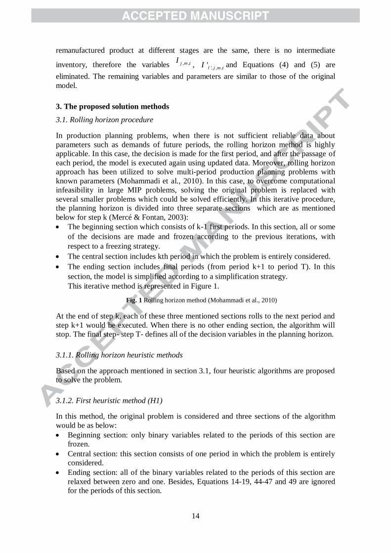
3. The proposed solution methods

3.1. Rolling horizon procedure

In production planning problems, when there is not sufficient reliable data about

parameters such as demands of future periods, the rolling horizon method is highly

applicable. In this case, the decision is made for the first period, and after the passage of

each period, the model is executed again using updated data. Moreover, rolling horizon

approach has been utilized to solve multi-period production planning problems with

known parameters (Mohammadi et al., 2010). In this case, to overcome computational

infeasibility in large MIP problems, solving the original problem is replaced with

several smaller problems which could be solved efficiently. In this iterative procedure,

the planning horizon is divided into three separate sections which are as mentioned

below for step k (Mercé & Fontan, 2003):

The beginning section which consists of k-1 first periods. In this section, all or some

of the decisions are made and frozen according to the previous iterations, with

respect to a freezing strategy.

The central section includes kth period in which the problem is entirely considered.

The ending section includes final periods (from period k+1 to period T). In this

section, the model is simplified according to a simplification strategy.

This iterative method is represented in Figure 1.

Fig. 1 Rolling horizon method (Mohammadi et al., 2010)

At the end of step k, each of these three mentioned sections rolls to the next period and

step k+1 would be executed. When there is no other ending section, the algorithm will

stop. The final step- step T- defines all of the decision variables in the planning horizon.

3.1.1. Rolling horizon heuristic methods

Based on the approach mentioned in section 3.1, four heuristic algorithms are proposed

to solve the problem.

3.1.2. First heuristic method (H1)

In this method, the original problem is considered and three sections of the algorithm

would be as below:

Beginning section: only binary variables related to the periods of this section are

frozen.

Central section: this section consists of one period in which the problem is entirely

considered.

Ending section: all of the binary variables related to the periods of this section are

relaxed between zero and one. Besides, Equations 14-19, 44-47 and 49 are ignored

for the periods of this section.

15

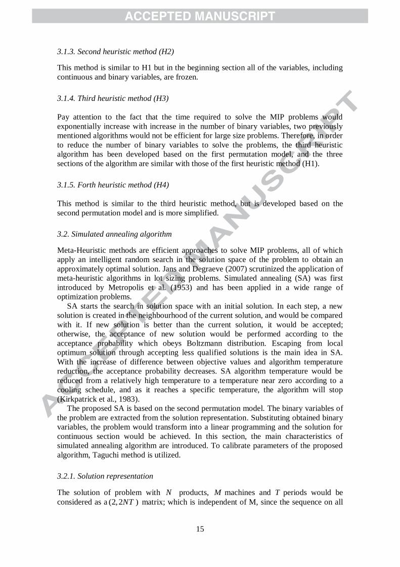
3.1.3. Second heuristic method (H2)

This method is similar to H1 but in the beginning section all of the variables, including

continuous and binary variables, are frozen.

3.1.4. Third heuristic method (H3)

Pay attention to the fact that the time required to solve the MIP problems would

exponentially increase with increase in the number of binary variables, two previously

mentioned algorithms would not be efficient for large size problems. Therefore, in order

to reduce the number of binary variables to solve the problems, the third heuristic

algorithm has been developed based on the first permutation model, and the three

sections of the algorithm are similar with those of the first heuristic method (H1).

3.1.5. Forth heuristic method (H4)

This method is similar to the third heuristic method, but is developed based on the

second permutation model and is more simplified.

3.2. Simulated annealing algorithm

Meta-Heuristic methods are efficient approaches to solve MIP problems, all of which

apply an intelligent random search in the solution space of the problem to obtain an

approximately optimal solution. Jans and Degraeve (2007) scrutinized the application of

meta-heuristic algorithms in lot sizing problems. Simulated annealing (SA) was first

introduced by Metropolis et al. (1953) and has been applied in a wide range of

optimization problems.

SA starts the search in solution space with an initial solution. In each step, a new

solution is created in the neighbourhood of the current solution, and would be compared

with it. If new solution is better than the current solution, it would be accepted;

otherwise, the acceptance of new solution would be performed according to the

acceptance probability which obeys Boltzmann distribution. Escaping from local

optimum solution through accepting less qualified solutions is the main idea in SA.

With the increase of difference between objective values and algorithm temperature

reduction, the acceptance probability decreases. SA algorithm temperature would be

reduced from a relatively high temperature to a temperature near zero according to a

cooling schedule, and as it reaches a specific temperature, the algorithm will stop

(Kirkpatrick et al., 1983).

The proposed SA is based on the second permutation model. The binary variables of

the problem are extracted from the solution representation. Substituting obtained binary

variables, the problem would transform into a linear programming and the solution for

continuous section would be achieved. In this section, the main characteristics of

simulated annealing algorithm are introduced. To calibrate parameters of the proposed

algorithm, Taguchi method is utilized.

3.2.1. Solution representation

The solution of problem with N products, M machines and T periods would be

considered as a (2,2 )NT matrix; which is independent of M, since the sequence on all

16

machines is assumed the same. The first row would represent the sequence of products

and processes; while the second row indicates whether the processes of a product in

each period have been executed. For product j , 2 1j and 2 j imply manufacturing

and remanufacturing, respectively. The value 1 in the second row represents the

execution of the corresponding process; while otherwise, it indicates that it is not

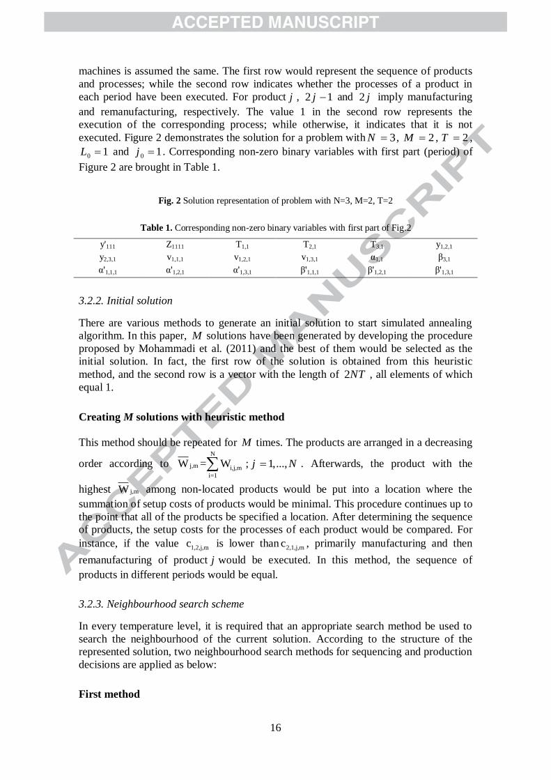
executed. Figure 2 demonstrates the solution for a problem with 3N , 2M , 2T ,

0 1L and 0 1j . Corresponding non-zero binary variables with first part (period) of

Figure 2 are brought in Table 1.

Fig. 2 Solution representation of problem with N=3, M=2, T=2

Table 1. Corresponding non-zero binary variables with first part of Fig.2

y1,2,1 T3,1

T2,1 T1,1

Z1111

y'111

β3,1 α1,1

v1,3,1 v1,2,1

v1,1,1 y2,3,1

β'1,3,1

β'1,2,1

β'1,1,1

α'1,3,1

α'1,2,1

α'1,1,1

3.2.2. Initial solution

There are various methods to generate an initial solution to start simulated annealing

algorithm. In this paper, M solutions have been generated by developing the procedure

proposed by Mohammadi et al. (2011) and the best of them would be selected as the

initial solution. In fact, the first row of the solution is obtained from this heuristic

method, and the second row is a vector with the length of 2NT , all elements of which

equal 1.

Creating M solutions with heuristic method

This method should be repeated for M times. The products are arranged in a decreasing

order according to N

j,m i,j,m

i=1

W = W ; 1,...,j N . Afterwards, the product with the

highest j,mW among non-located products would be put into a location where the

summation of setup costs of products would be minimal. This procedure continues up to

the point that all of the products be specified a location. After determining the sequence

of products, the setup costs for the processes of each product would be compared. For

instance, if the value 1,2,j,mc is lower than 2,1,j,mc , primarily manufacturing and then

remanufacturing of product j would be executed. In this method, the sequence of

products in different periods would be equal.

3.2.3. Neighbourhood search scheme

In every temperature level, it is required that an appropriate search method be used to

search the neighbourhood of the current solution. According to the structure of the

represented solution, two neighbourhood search methods for sequencing and production

decisions are applied as below:

First method

17

In this method which is utilized to improve the sequence of products and processes,

period t is first randomly selected. Thereafter, a ( , , )l j t and a ( , , )k i t are randomly

chosen, and would be swapped in a column form.

Second method

This method is applied to determine decisions about execution of manufacturing and

remanufacturing of products. A ( , , )l j t would be randomly chosen. If the value of the

selected array is 1, it would change to zero, and vice versa.

In each temperature, neighbourhood search would be repeated for 2N times. If the

number of accepted solutions in any temperature exceeds a specific value, the search in

that temperature would stop. The first and the second methods would be applied with

specific probabilities P and 1-P, respectively.

3.2.4. Cooling schedule

Temperature would gradually decrease through the progress of the algorithm from a

high value

( iT ) to a temperature near zero with a specific pattern which is defined as bellow:

1i iT T (52)

where α (0,1) is a constant value.

3.2.5. Termination criterion

If fT< T , or the specific number of accepted solutions in several consecutive

temperatures equals zero, the SA algorithm will stop.

3.2.6. Attitude of encountering constraints

In the proposed model, manufacturing and remanufacturing of each product are planned

to be performed consecutively. To create a feasible solution, it is required that the arrays

corresponding to manufacturing and remanufacturing of each product be consecutive in

each solution. Regarding the act of first neighbourhood search method, this order might

not be obeyed. Consequently, to create a feasible solution a repair procedure has been

applied to modify the obtained solution. In this approach for each array, if the array

relates to the manufacturing (remanufacturing) process of a product, the array

corresponding to the remanufacturing (manufacturing) process of the same product

would be located right after that, and the rest arrays between these two arrays, would

move to the right. To encounter the demand and capacity constraints, a penalty attitude

has been considered. In this regard, Equations (3), (8) and (9) are replaced with

Equations (53), (54) and (55), respectively.

, 1 ', , ' , , , ,

' '

1 ( (1 ). ' ) / ;

1,..., ; 1,...,

L L

j t l j j t l j t j t j t j t

l l

Is r x x Is d dr

j N t T

(53)

18

, , , , ,( / ) 1 ; 1,..., ; 1,..., ; 1,...,j m t m t j m tco C vr j N m M t T

(54)

, , , , ,( ' / ) 1 ' ; 1,..., ; 1,..., ; 1,...,j m t m t j m tco C vr j N m M t T

(55)

where ,j tdr is a positive variable which indicates the violation of the demand constraint

and , ,j m tvr and

, ,' j m tvr are positive variables to demonstrate violation of the capacity

constraints.

By considering significant penalty in objective function for violation of demand and

capacity constraints as mentioned in Equation (56), algorithm will lead toward finding

feasible solutions.

'

, , , , ,

1 1 1 1 1

* *N M T N T

j m t j m t j t

j m t j t

bigM vr vr bigM dr

(56)

where bigM indicates the penalty cost per unit of constraint violation.

3.2.7. Parameter calibration

Design of parameters of meta-heuristic algorithms is a fundamentally factor on the

efficiency of the algorithm, since an inappropriate selection of algorithm parameters

would lead to its weak performance. In this paper, Taguchi method has been applied to

calibrate the proposed algorithm parameters. Orthogonal arrays in Taguchi method

permit the analysis of numerous factors with a small number of experiments. In this

method, performance measure called signal-to-noise (S/N) ratio is maximized to obtain

the optimum level of factors. The term ‘signal’ represents the desirable value (response

variable) and ‘noise’ represents the undesirable value (standard deviation). The S/N

ratio indicates the mean-square deviation present in the response variable (Taguchi et

al., 2000). Taguchi method acts as mentioned below, to calibrate the parameters (Wu &

Hamada, 2011):

For each experiment, S/N ratio is calculated.

For factors which have a significant impact on S/N ratio, the level that maximizes

the S/N ratio is optimum.

For factors which do not have a noticeable impact on S/N ratio but affect response

variable mean, the best level retains the best objective function.

For factors which affect neither S/N ratio, nor the response variable mean, a level

with the lowest calculation time would be selected.

The utilized response variable in this paper is Relative Percentage Deviation (RPD)

which is preferred to be minimized and defined as below:

min

min

100ii

OF OFRPD

OF

(57)

where minOF is the best found objective value for a specific problem, and iOF is the

obtained objective value for ith

trial. Since the lower values of response variable are

preferred, S/N ratio is defined as below:

2

1

1/ 10log( )

n

i

i

S N RPDn

(58)

where n is the number of replications.

19

By recognizing the effective parameters on the efficiency of simulated annealing

algorithm, calibration of following parameters are considered:

Cooling rate : two levels (0.95, 0.975)

Initial temperature: three levels (75, 100, 125)

Final temperature: three levels (0.05Ti, 0.075Ti, 0.1Ti)

Number of neighborhood search: three levels (20, 35, 50)

Probability of neighborhood search change: (0.4, 0.5, 0.6)

Number of accepted solutions in each temperature to stop the search: three levels (6,

8, 10)

According to the considered levels and factors, the full factorial experiment design

for mentioned six factors requires 35×2

1=486 experiments. But, regarding statistical

theories, it is not necessary to perform all the experiments. Therefore, fractional

replicated designs are used in this study. To select proper orthogonal array, it is needed

to calculate the degree of freedom. In the current study, 1 degree of freedom for total

mean, 1 degree of freedom for the factor with 2 levels and 2 degrees of freedom for

each factor with three levels (2×5=10) are required. Thus, the sum of required degree of

freedom would be 1+1+2×5=12. Hence, the appropriate array must have at least 12

rows. The selected orthogonal array should be able to incorporate the factor level

combinations in the experiment. Therefore, orthogonal array L18 (21*3

7) is appropriate

to implement in this study. Orthogonal arrays layout for parameter design can be seen in

study conducted by Wu and Wu (2000).

Since there are five factors with 3 levels in the current study, according to Taguchi

experimental design procedure, two columns could be remained empty. For each

experiment of orthogonal array L18, each of the problems given in Table 2 has been

created using parameters introduced in Table 3, and has been solved for 5 times. Thus, a

total number of 18×5×5= 450 problems have been solved.

Table 2. The size of problems used in calibration of parameters

Table 3. The parameters of the problem

dj,t ~ U(0,180), ul’,j,t ~ U(0,90/L), bj,m ~ U(1.5,2),b’l’,j,m ~ (0.4+(l’-1)p)× U(1.5,2), hj,m ~ U(0.2,0.4), h’l’,j,m ~ U(0.15,0.3), hrl’,j ~ U(0.1,0.2),hsj ~ U(0.4,0.8), pj,m,t ~ U(1.5,2),p’l’,j,m ~ (0.4+(l’-1)p)× U(1.5,2),

Wi,j,m ~ U(35,70), Si,j,m ~ U(35,70),rl,k,j,m ~ U(5,10), cl,k,j,m ~ U(5,10),αrl’,j ~ U(0.01,0.02), Cm,t ~ U(am,bm);

p=(0.6-0.4)/(L-1), am= 300N+ 200(m-1),bm =300N+ 300(m-1)

S/N ratio and RPD mean value for SA are demonstrated in Figure 3 and Figure 4,

respectively.

Fig.3 The mean of S/N ratio at each level of the SA parameters

Fig. 4 The mean of RPD at each level of the SA parameters

According to these figures, Table 4 gives the best levels of factors for this algorithm.

Table 4. Best levels of the factors for proposed SA

The optimum level Parameter

0.975 Cooling rate (α )

100 Initial temperature (Ti)

15×15×15 10×10×10 7×7×7 5×5×5 3×3×3

20

0.05Ti

Final temperature (Tf)

50 Number of neighborhood search (NS length)

0.6 Probability of neighborhood search change (P)

8 The number of accepted solutions in each

temperature to stop searching in that temperature

(NA)

4. Numerical experiments

To evaluate the efficiency of proposed SA to solve the considered problem,

computational experiments have been conducted. To compare the performance of

heuristic methods and SA about solution quality and solution time, 24 problems with

sizes from 3 3 3N M T to 15 15 15N M T are solved. The number

of quality level is considered as 3 in all instances. The proposed model and MIP-based

heuristics are coded by GAMS IDE (ver. 24.1.3) software, using CPLEX solver, and SA

is coded by MATLAB 2013. The required parameters of the problem have been

obtained by Uniform distributions and are as given in Table 3. All of the problems have

been executed on a PC with a Core i5 2.53 GHz CPU and a 4GB RAM.

To obtain trustworthy solutions, each problem has been solved for 5 times with

proposed SA method and the best results have been reported. The computational results

including objective value and solution time obtained by algorithms for all instances

have been cited in Table 5. Moreover, the objective values of algorithms are compared

with the exact solutions for small instances.

Table 5. Computational results for proposed algorithms

SA H4 H3 H2 H1 Exact solution Problem

size

(N.M.T)

CPU

time obj

CPU

time obj

CPU

time obj

CPU

time obj

CPU

time obj

CPU

time obj

9.037 4871.86

(1.06%) 10.9

4871.86

(1.06%) 11.57

4866.93

(0.95%) 8.54

4948.26

(2.64%) 251.26

4821.00

(0%) 386.56 4821.00 3×3×3

10.96 5137.14

(1.48%) 11.46

5143.41

(1.60%) 12.07

5133.7

(1.41%) 10.86

5338.72

(5.46%) 267.59

5062.20

(0%) 411.67 5062.20 3×4×3

12.68 5003.96

(0.35%) 11.87

5003.96

(0.35%) 13.66

5003.47

(0.34%) 11.04

5199.08

(4.26%) 342.87

4986.55

(0%) 487.15 4986.55 3×3×4

16.96 4787.43

(0.70%) 12.96

4770.46

(0.34%) 18.33

4769.28

(0.32%) 10.68

5033.23

(5.87%) 306.99

4754.19

(0%) 466.55 4754.19 3×3×4

25.27 9008.39

(0.12%) 133.18

9008.39

(0.12%) 133.39

9008.34

(0.12%) 92.44

9389.92

(4.36%) 5504.56

9204.28

(2.3%) 7200* 8997.38 4×4×4

15.43 6768.17

(1.80%) 14.95

6723.23

(1.13%) 22.02

6702.75

(0.82%) 14.92

6999.45

(5.28%) 1258.45

6648.47

(0%) 1284.63 6648.47 3×5×3

17.13 7064.26

(1.04%) 13.27

7064.26

(1.04%) 16.38

7036.81

(0.65%) 11.05

7093.84

(1.47%) 383.05

6991.35

(0%) 538.50 6991.35 3×3×5

22.57 6920.7

(0.50%) 20.25

6920.7

(0.50%) 24.11

6918.17

(0.46%) 11.7

7240.04

(5.13%) 570.56

6886.54

(0%) 690.99 6886.54 3×3×5

46.43 17433.09

(0.83%) 126.05

17447.04

(0.91%) 414.82

17437.3

(0.86%) 2898.97

18362.71

(6.21%) 7200*

18082.6

(4.59%) 7200* 17289.3 5×5×5

76.01 27935.43 5770.2 28489.51 5771.53 28535.81 7200* 29348.98 - - -- 7×5×5

90.36 28643.25 424.45 28777.21 1740.73 28711.11 3382.73 29654.28 - -- 5×7×5

57.72 29853.43 3736.67 29711.00 5117.56 29958.18 3288.28 31048.24 - - -- 5×5×7

123.08 50308.88 6184.2 50371.95 6190.10 50347.99 - - - - -- 7×7×7

83.1 39868.76 5773.28 40048.4 5773.66 39834.49 - - - - -- 10×5×5

111.99 39926.76 2952.71 40344.79 4595.03 40329.29 - - - - -- 5×10×5

66.88 37160.67 5105.58 36968.74 5222.82 37233.20 - - - - -- 5×5×10

252.05 78533.52 6189.16 82673.58 6194.2 87320.8 - - - - -- 10×7×7

214.27 77125.21 6187.24 80626.737 6192.68 84602.45 - - - - -- 7×10×7

21

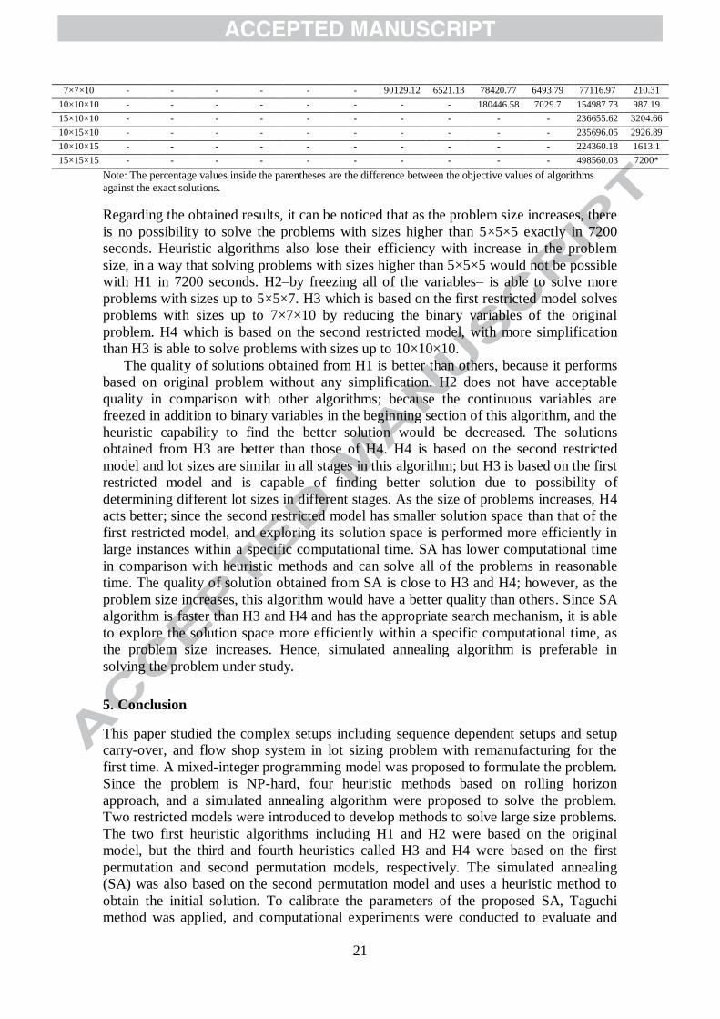
210.31 77116.97 6493.79 78420.77 6521.13 90129.12 - - - - -- 7×7×10

987.19 154987.73 7029.7 180446.58 - - - - - - -- 10×10×10

3204.66 236655.62 - - - - - - - - -- 15×10×10

2926.89 235696.05 - - - - - - - - -- 10×15×10

1613.1 224360.18 - - - - - - - - -- 10×10×15

7200* 498560.03 - - - - - - - - -- 15×15×15

Note: The percentage values inside the parentheses are the difference between the objective values of algorithms against the exact solutions.

Regarding the obtained results, it can be noticed that as the problem size increases, there

is no possibility to solve the problems with sizes higher than 5×5×5 exactly in 7200

seconds. Heuristic algorithms also lose their efficiency with increase in the problem

size, in a way that solving problems with sizes higher than 5×5×5 would not be possible

with H1 in 7200 seconds. H2–by freezing all of the variables– is able to solve more

problems with sizes up to 5×5×7. H3 which is based on the first restricted model solves

problems with sizes up to 7×7×10 by reducing the binary variables of the original

problem. H4 which is based on the second restricted model, with more simplification

than H3 is able to solve problems with sizes up to 10×10×10.

The quality of solutions obtained from H1 is better than others, because it performs

based on original problem without any simplification. H2 does not have acceptable

quality in comparison with other algorithms; because the continuous variables are

freezed in addition to binary variables in the beginning section of this algorithm, and the

heuristic capability to find the better solution would be decreased. The solutions

obtained from H3 are better than those of H4. H4 is based on the second restricted

model and lot sizes are similar in all stages in this algorithm; but H3 is based on the first

restricted model and is capable of finding better solution due to possibility of

determining different lot sizes in different stages. As the size of problems increases, H4

acts better; since the second restricted model has smaller solution space than that of the

first restricted model, and exploring its solution space is performed more efficiently in

large instances within a specific computational time. SA has lower computational time

in comparison with heuristic methods and can solve all of the problems in reasonable

time. The quality of solution obtained from SA is close to H3 and H4; however, as the

problem size increases, this algorithm would have a better quality than others. Since SA

algorithm is faster than H3 and H4 and has the appropriate search mechanism, it is able

to explore the solution space more efficiently within a specific computational time, as

the problem size increases. Hence, simulated annealing algorithm is preferable in

solving the problem under study.

5. Conclusion

This paper studied the complex setups including sequence dependent setups and setup

carry-over, and flow shop system in lot sizing problem with remanufacturing for the

first time. A mixed-integer programming model was proposed to formulate the problem.

Since the problem is NP-hard, four heuristic methods based on rolling horizon

approach, and a simulated annealing algorithm were proposed to solve the problem.

Two restricted models were introduced to develop methods to solve large size problems.

The two first heuristic algorithms including H1 and H2 were based on the original

model, but the third and fourth heuristics called H3 and H4 were based on the first

permutation and second permutation models, respectively. The simulated annealing

(SA) was also based on the second permutation model and uses a heuristic method to

obtain the initial solution. To calibrate the parameters of the proposed SA, Taguchi

method was applied, and computational experiments were conducted to evaluate and

22

compare the developed heuristic methods and SA algorithm. According to the

numerical experiments, the problems with sizes higher than 5×5×5 could not be solved

exactly in 7200 seconds. H1 is not possible to solve the problems with sizes higher than

5×5×5 in 7200 seconds. H2 is able to solve problems with sizes up to 5×5×7. H3 solves

the problems with sizes up to 7×7×10 and H4 is able to solve problems with sizes up to

10×10×10. The quality of H1 solutions is better than other heuristics, and H2 has the

worst quality among others. H3 performs better than H4; but as the size of problems

increases, H4 acts better. SA is faster in comparison with heuristic methods and can

solve all of the problems in reasonable time. The quality of SA solution is close to H3

and H4; however, SA performs better for large instances. Therefore, SA algorithm is

suggested to solve the problem under study.

This study could be implemented in complicated industries such as car factories.

Remanufacturing is important from an economic point of view; additionally it could be

reduce the usage of raw material and is interesting environmentally. Performing

remanufacturing using returned products is possible by improving reverse logistic and

using incentive policies such as refunds to gather returned products. It should be noted

that these activities have their own special considerations and may cause additional

costs which should be concerned.

The issue of uncertainties in remanufacturing such as the quality, amount of returned

products, and processing time could be a development to the current study.

Additionally, modelling and solving this problem as a multi-objective problem,

considering scheduling objectives such as minimizing the maximum completion time

(makespan) besides the cost minimization, is suggested for further research.

References

Almada-Lobo, B. and James, R.J. (2010). Neighbourhood search meta-heuristics for capacitated lot-sizing with sequence-dependent setups. International Journal of Production

Research, 48(3), 861-878.

Almada-Lobo, B., Klabjan, D., Antónia carravilla, M. and Oliveira, J.F. (2007). Single machine multi-product capacitated lot sizing with sequence-dependent setups. International

Journal of Production Research, 45(20), 4873-4894.

Bahl, H.C., Ritzman, L.P. and Gupta, J.N. (1987). OR Practice—Determining Lot Sizes and Resource Requirements: A Review. Operations Research, 35(3), 329-345.

Baki, M.F., Chaouch, B.A. and Abdul-Kader, W. (2014). A heuristic solution procedure for the

dynamic lot sizing problem with remanufacturing and product recovery. Computers &

Operations Research, 43, 225-236. Chen, M. and Abrishami, P. (2014). A mathematical model for production planning in hybrid

manufacturing-remanufacturing systems. The International Journal of Advanced

Manufacturing Technology, 71(5-8), 1187-1196. Corominas, A., Lusa, A. and Olivella, J. (2012). A manufacturing and remanufacturing

aggregate planning model considering a non-linear supply function of recovered

products. Production Planning & Control, 23(2-3), 194-204.

Dong, M., Lu, S. and Han, S. (2011). Production planning for hybrid remanufacturing and manufacturing system with component recovery. In: Advances in Electrical

Engineering and Electrical Machines (pp. 511-518): Springer.

Gómez Urrutia, E.D., Aggoune, R. and Dauzère-Pérès, S. (2014). Solving the integrated lot-sizing and job-shop scheduling problem. International Journal of Production Research,

52(17), 5236-5254.

Gupta, D. and Magnusson, T. (2005). The capacitated lot-sizing and scheduling problem with sequence-dependent setup costs and setup times. Computers & Operations Research,

32(4), 727-747.

23

Hilger, T., Sahling, F. and Tempelmeier, H. (2015). Capacitated dynamic production and

remanufacturing planning under demand and return uncertainty. OR Spectrum, 1-28.

Ilgin, M.A. and Gupta, S.M. (2010). Environmentally conscious manufacturing and product

recovery (ECMPRO): a review of the state of the art. Journal of environmental management, 91(3), 563-591.

James, R.J. and Almada-Lobo, B. (2011). Single and parallel machine capacitated lotsizing and

scheduling: New iterative MIP-based neighborhood search heuristics. Computers & Operations Research, 38(12), 1816-1825.

Jans, R. and Degraeve, Z. (2007). Meta-heuristics for dynamic lot sizing: A review and

comparison of solution approaches. European Journal of Operational Research, 177(3), 1855-1875.

Jing, Y., Li, W., Wang, X. and Deng, L. (2016). Production planning with remanufacturing and

back-ordering in a cooperative multi-factory environment. International Journal of

Computer Integrated Manufacturing, 29(6), 692-708. Karimi, B., Fatemi Ghomi, S.M.T. and Wilson, J. (2003). The capacitated lot sizing problem: a

review of models and algorithms. Omega, 31(5), 365-378.

Kenne, J.-P., Dejax, P. and Gharbi, A. (2012). Production planning of a hybrid manufacturing–remanufacturing system under uncertainty within a closed-loop supply chain.

International Journal of Production Economics, 135(1), 81-93.

Kirkpatrick, S., Gelatt, C.D. and Vecchi, M.P. (1983). Optimization by simmulated annealing. science, 220(4598), 671-680.

Kovács, A., Brown, K.N. and Tarim, S.A. (2009). An efficient MIP model for the capacitated

lot-sizing and scheduling problem with sequence-dependent setups. International

Journal of Production Economics, 118(1), 282-291. Lee, C.-W., Doh, H.-H. and Lee, D.-H. (2015). Capacity and production planning for a hybrid

system with manufacturing and remanufacturing facilities. Proceedings of the

Institution of Mechanical Engineers, Part B: Journal of Engineering Manufacture, 229(9), 1645-1653.

Li, X., Baki, F., Tian, P. and Chaouch, B.A. (2014). A robust block-chain based tabu search

algorithm for the dynamic lot sizing problem with product returns and remanufacturing.

Omega, 42(1), 75-87. Li, X., Li, Y. and Saghafian, S. (2013). A hybrid manufacturing/remanufacturing system with

random remanufacturing yield and market-driven product acquisition. Engineering

Management, IEEE Transactions on, 60(2), 424-437. Li, Y., Chen, J. and Cai, X. (2006). Uncapacitated production planning with multiple product

types, returned product remanufacturing, and demand substitution. OR Spectrum, 28(1),

101-125. Macedo, P.B., Alem, D., Santos, M., Junior, M.L. and Moreno, A. (2016). Hybrid

manufacturing and remanufacturing lot-sizing problem with stochastic demand, return,

and setup costs. The International Journal of Advanced Manufacturing Technology,

82(5-8), 1241-1257. Menezes, A.A., Clark, A. and Almada-Lobo, B. (2011). Capacitated lot-sizing and scheduling

with sequence-dependent, period-overlapping and non-triangular setups. Journal of

Scheduling, 14(2), 209-219. Mercé, C. and Fontan, G. (2003). MIP-based heuristics for capacitated lotsizing problems.

International Journal of Production Economics, 85(1), 97-111.

Metropolis, N., Rosenbluth, A.W., Rosenbluth, M.N., Teller, A.H. & Teller, E. (1953). Equation of state calculations by fast computing machines. The journal of chemical

physics, 21(6), 1087-1092.

Mohammadi, M. (2010). Integrating lotsizing, loading, and scheduling decisions in flexible

flow shops. The International Journal of Advanced Manufacturing Technology, 50(9-12), 1165-1174.

Mohammadi,M.,Fatemi Ghomi,S.M.T.,and Jafari, N. (2011). A genetic algorithm for

simultaneous lotsizing and sequencing of the permutation flow shops with sequence-

24

dependent setups. International Journal of Computer Integrated Manufacturing, 24(1),

87-93.

Mohammadi, M., Fatemi Ghomi, S.M.T., Karimi, B. and Torabi, S.A. (2010). Rolling-horizon

and fix-and-relax heuristics for the multi-product multi-level capacitated lotsizing problem with sequence-dependent setups. Journal of Intelligent Manufacturing, 21(4),

501-510.

Mohammadi, M. and Jafari, N. (2011). A new mathematical model for integrating lot sizing, loading, and scheduling decisions in flexible flow shops. The International Journal of

Advanced Manufacturing Technology, 55(5-8), 709-721.

Mukhopadhyay, S.K. and Ma, H. (2009). Joint procurement and production decisions in remanufacturing under quality and demand uncertainty. International Journal of

Production Economics, 120(1), 5-17.

Naeem, M.A., Dias, D.J., Tibrewal, R., Chang, P.-C. and Tiwari, M.K. (2013). Production

planning optimization for manufacturing and remanufacturing system in stochastic environment. Journal of Intelligent Manufacturing, 24(4), 717-728.

Pan, Z., Tang, J. and Liu, O. (2009). Capacitated dynamic lot sizing problems in closed-loop

supply chain. European Journal of Operational Research, 198(3), 810-821. Parsopoulos, K.E., Konstantaras, I. and Skouri, K. (2015). Metaheuristic optimization for the

single-item dynamic lot sizing problem with returns and remanufacturing. Computers &

Industrial Engineering, 83, 307-315. Pineyro, P. and Viera, O. (2010). The economic lot-sizing problem with remanufacturing and

one-way substitution. International Journal of Production Economics, 124(2), 482-488.

Ramezanian, R. and Saidi-Mehrabad, M. (2013). Hybrid simulated annealing and MIP-based

heuristics for stochastic lot-sizing and scheduling problem in capacitated multi-stage production system. Applied Mathematical Modelling, 37(7), 5134-5147.

Ramezanian, R., Saidi-Mehrabad, M. and Teimoury, E. (2013). A mathematical model for

integrating lot-sizing and scheduling problem in capacitated flow shop environments. The International Journal of Advanced Manufacturing Technology, 66(1-4), 347-361.

Ramezanian, R., Sanami, S.F. and Nikabadi, M.S. (2016). A simultaneous planning of

production and scheduling operations in flexible flow shops: case study of tile industry.

The International Journal of Advanced Manufacturing Technology, 1-15. Richter, K. and Weber, J. (2001). The reverse Wagner/Whitin model with variable

manufacturing and remanufacturing cost. International Journal of Production

Economics, 71(1), 447-456. Shi, J., Zhang, G., Sha, J. and Amin, S.H. (2010). Coordinating production and recycling

decisions with stochastic demand and return. Journal of Systems Science and Systems

Engineering, 19(4), 385-407. Sifaleras, A. and Konstantaras, I. (2015). General variable neighborhood search for the multi-

product dynamic lot sizing problem in closed-loop supply chain. Electronic Notes in

Discrete Mathematics, 47(1), 69-76.

Stindt, D. and Sahamie, R. (2014). Review of research on closed loop supply chain management in the process industry. Flexible Services and Manufacturing Journal, 26(1-2), 268-293.

Taguchi, G., Chowdhury, S. and Taguchi, S. (2000). Robust engineering: McGraw-Hill

Professional. Teunter, R.H., Bayindir, Z.P. and Den Heuvel, W.V. (2006). Dynamic lot sizing with product

returns and remanufacturing. International Journal of Production Research, 44(20),

4377-4400. Wagner, H.M. and Whitin, T.M. (1958). Dynamic version of the economic lot size model.

Management science, 5(1), 89-96.

Wei, C., Li, Y. and Cai, X. (2011). Robust optimal policies of production and inventory with

uncertain returns and demand. International Journal of Production Economics, 134(2), 357-367.

Wolosewicz, C., Dauzère-Pérès, S. & Aggoune, R. (2015). A Lagrangian heuristic for an

integrated lot-sizing and fixed scheduling problem. European Journal of Operational Research, 244(1), 3-12.

25

Wu, C.J. & Hamada, M.S. (2011). Experiments: planning, analysis, and optimization (Vol.

552): John Wiley & Sons.

Wu, Y. & Wu, A. (2000). Taguchi methods for robust design: American Society of Mechanical

Engineers.

Yang, J., Golany, B. & Yu, G. (2005). A concave‐cost production planning problem with

remanufacturing options. Naval Research Logistics (NRL), 52(5), 443-458.

Zhang, J., Liu, X. & Tu, Y. (2011). A capacitated production planning problem for closed-loop supply chain with remanufacturing. The International Journal of Advanced

Manufacturing Technology, 54(5-8), 757-766.

Zhang, Z.-H., Jiang, H. & Pan, X. (2012). A Lagrangian relaxation based approach for the capacitated lot sizing problem in closed-loop supply chain. International Journal of

Production Economics, 140(1), 249-255.

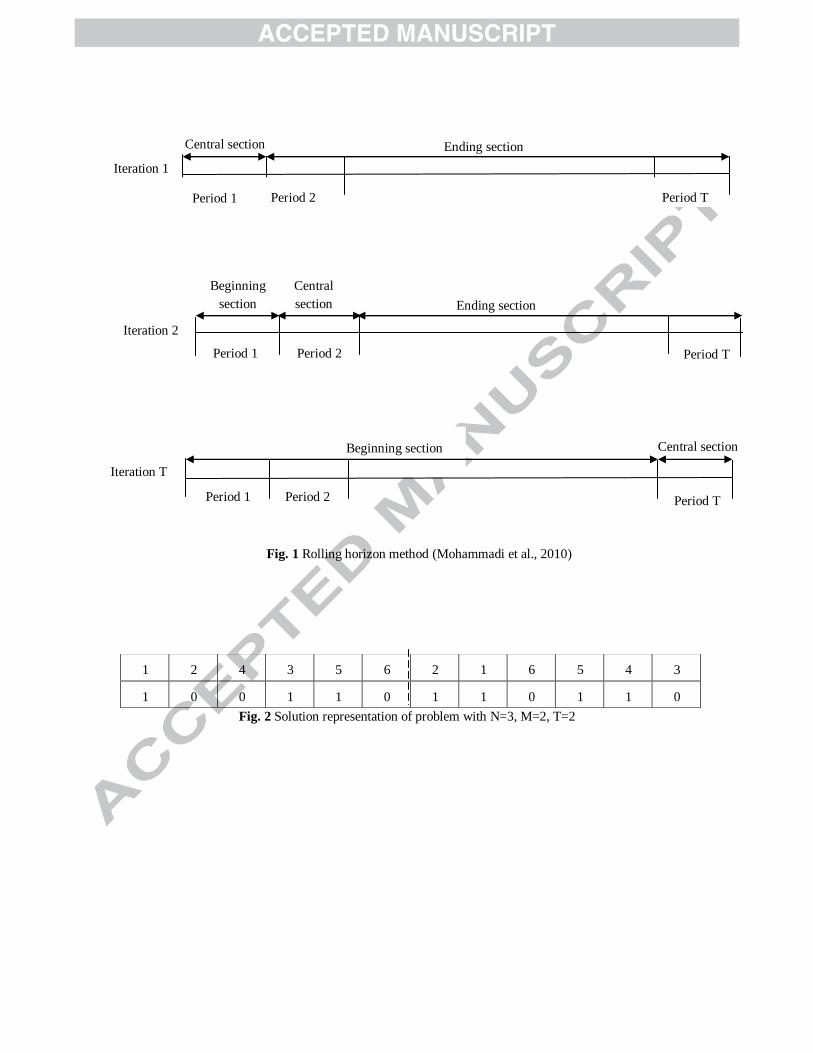
Fig. 1 Rolling horizon method (Mohammadi et al., 2010)

Fig. 2 Solution representation of problem with N=3, M=2, T=2

3 4 5 6 1 2 6 5 3 4 2 1

0 1 1 0 1 1 0 1 1 0 0 1

Period 1 Period 2 Period T

Beginning section

Iteration T

Central section

Period T Period 2 Period 1

Iteration 2

Central

section

Beginning

section Ending section

Central section

Iteration 1

Ending section

Period 2 Period T Period 1

Fig.3 The mean of S/N ratio at each level of the SA parameters

Fig.4 The mean of RPD at each level of the SA parameters

26

Research highlights

A multi-stage lot sizing problem with remanufacturing is modeled.

Sequence dependent setups and setup carry-over in a flow shop are considered.

A mixed integer programming is introduced to formulate the problem.

Rolling horizon heuristics and a SA algorithm are proposed to solve the model.

For large size problems SA algorithm would have better solutions than heuristics.