MSH3 Generalized Linear model (Part 1) · MSH3 Generalized Linear model (Part 1) Jennifer S.K. CHAN...

MSH3 Generalized Linear model (Part 1)

Jennifer S.K. CHAN

Course outline

Part I: Generalized Linear Model

1. Maximum Likelihood Inference

Newton-Raphson and Fisher Scoring methods, Expectation Max-imization (EM), Monte Carlo EM and Expectation ConditionalMaximization (ECM) algorithms

2. Exponential Family

Generalized linear models; Exponential family, Weighted leastsquares; ML estimation, Quasi-likelihood, Random effects mod-els.

3. Model Selection

Deviance for Likelihood Ratio Tests, Wald Tests, Akaike’s in-formation criterion (AIC) and Bayesian information criterion(BIC), Examples.

4. Survival Analysis

Kaplan-Meier estimator, Proportional hazards models, Cox’sproportional hazards models.

MSH3 Generalized linear model

Contents

§1 Maximum likelihood Inference 2§1.1 Motivating examples . . . . . . . . . . . . . . . . . . . 2§1.2 Likelihood function . . . . . . . . . . . . . . . . . . . . 6§1.3 Score vector . . . . . . . . . . . . . . . . . . . . . . . . 8§1.4 Information matrix . . . . . . . . . . . . . . . . . . . . 9§1.5 Newton-Raphson and Fisher Scoring methods . . . . . 12§1.6 Expectation Maximization (EM) algorithm . . . . . . 16

§1.6.1 Basic EM algorithm . . . . . . . . . . . . . . . 16§1.6.2 Monte Carlo EM Algorithm . . . . . . . . . . . 26§1.6.3 Expectation Conditional Maximization (ECM)

algorithm . . . . . . . . . . . . . . . . . . . . . 30§1.7 Appendix for EM algorithm . . . . . . . . . . . . . . . 37

SydU MSH3 GLM (2013) Second semester Dr. J. Chan 1

MSH3 Generalized linear model Ch.1 Max. likelihood inf.

§1 Maximum likelihood Inference

§1.1 Motivating examples

AIDS deaths (counts)

The numbers of death Yi from AIDS in Australia for three-monthperiods from 1983 to 1986 are shown below.

The Poisson regression model

Yi ∼ Poisson(µi), with µi = exp(a+ bti) > 0

is fitted and the maximum likelihood (ML) estimates are a = 0.376and b = 0.254. For each 3-month period, there will be a 29.3%(exp(0.254) = 1.293) increase in expected AIDS deaths. Note thatthe variance increases with the mean and the log link function g(µi) =ln(µi) = β′xi is used.

> no=c(0,1,2,3,1,5,10,17,23,31,20,25,37,45)

> time=c(1:14)

> poi=glm(no~time, family=poisson(link=log))

> summary(poi)

Call:

glm(formula = y ~ x, family = poisson(link = log))

Deviance Residuals:

Min 1Q Median 3Q Max

-2.2502 -0.9815 -0.6770 0.2545 2.6731

Coefficients:

Estimate Std. Error z value Pr(>|z|)

(Intercept) 0.37571 0.24884 1.51 0.131

x 0.25365 0.02188 11.60 <2e-16 ***

---

Signif. codes: 0 ’***’ 0.001 ’**’ 0.01 ’*’ 0.05 ’.’ 0.1 ’ ’ 1



(Dispersion parameter for poisson family taken to be 1)

Null deviance: 203.549 on 13 degrees of freedom

Residual deviance: 28.169 on 12 degrees of freedom

AIC: 85.358

Number of Fisher Scoring iterations: 5

> par=poi$coeff

> names(par)=NULL

> par

[1] 0.3757110 0.2536485

> beta0=par[1]

> beta1=par[2]

> par(mfrow=c(2,2))

> c1=function(time) exp(beta0+beta1*time)

> plot(time,no,pch=20,col=’blue’ )

> curve(c1,1,14,add=TRUE)

> title("Poisson regression")

Mice data

Twenty six mice were given different level xi of drug. Outcomes Yi arewhether they responded to the drug (Yi = 1) or not (Yi = 0).

The logistic regression model for binary data is

Yi ∼ Bernoulli(µi), with logit(µi) = ln

(µi

1− µi

)= a+ bxi.

Note that

ln

(µi

1− µi

)= a+ bxi ⇒ µi =

ea+bxi

1 + ea+bxi.

> y=c(0,0,0,0,0,1,0,0,0,0,1,0,1,0,0,1,1,1,1,1,1,1,1,1,1,1)



> dose=c(0:25)/10

> log=glm(y~dose, family=binomial(link=logit))

> summary(log)

Call:

glm(formula = y ~ dose, family = binomial(link = logit))

Deviance Residuals:

Min 1Q Median 3Q Max

-1.5766 -0.4757 0.1376 0.4129 2.1975

Coefficients:

Estimate Std. Error z value Pr(>|z|)

(Intercept) -4.111 1.638 -2.510 0.0121 *

dose 3.581 1.316 2.722 0.0065 **

---

Signif. codes: 0 ’***’ 0.001 ’**’ 0.01 ’*’ 0.05 ’.’ 0.1 ’ ’ 1

(Dispersion parameter for binomial family taken to be 1)

Null deviance: 35.890 on 25 degrees of freedom

Residual deviance: 17.639 on 24 degrees of freedom

AIC: 21.639

Number of Fisher Scoring iterations: 6

> par=log$coeff

> names(par)=NULL

> par

[1] -4.111361 3.581176

> beta0=par[1]

> beta1=par[2]

> c1=function(dose) exp(beta0+beta1*dose)/(1+exp(beta0+beta1*dose))

> plot(dose,y, pch=20,col=’red’)

> curve(c1,0,2.5,add=TRUE)

> title("Logistic regression")

For parameter estimation, the nonparametric LSE , the parametricmaximum likelihood (ML, PML, QML, GEE, EM, MCEM, etc) andBayesian methods methods will be discussed. Kernel smoothing andother semi-parametric methods are not included. Model selection is



based on Akaike Information criterion (AIC), Bayesian Informationcriterion (BIC) and the Deviance information criterion (DIC).

For application, the two examples analyse counts data with Pois-son distribution and binary data with Bernounill distribution respec-tively. Others include categorial data with multinominal distributionand positive continuous data with Weibull distribution. These illus-trate different data distributions under the Exponential Family. Themean of the data distribution is linked to a linear function of covari-ates with possibly random effects but the variance is NOT modelled.Popular time series models with heteroskedastic variance and longmemory such as Generalized autoregressive conditional heteroskedas-tic (GARCH) model and stochastic volatility (SV) model will not beconsidered.



§1.2 Likelihood function

Let Y1, . . . , Yn be n independent random variables (rv) with probabilitydensity functions (pdf) f(yi,θ) depending on a vector-value parameterθ. The joint density of y = (y1, . . . , yn)′

f(y|θ) =n∏i=1

f(yi|θ) = L(θ;y)

as a function of unknown parameter θ given y is called the likeli-hood function. We often work with the logarithm of f(y,θ), the log-likelihood function:

`(θ;y) = lnL(θ;y) =n∑i=1

ln f(yi|θ).

The maximum-likelihood (ML) estimator θ maximzes the log-likelihoodfunction given the data y, that is,

`(θ;y) ≥ `(θ;y) for all θ.

In other words, they make the observed data as likely as possible underthe model.

Example: The log-likelhood function for Geometric Distribution.Consider a series of independent Bernoulli trials with a common prob-ability of success π. The distribution for the number of failures Yibefore the first success has a pdf

Pr(Yi = yi) = (1− π)yiπ

for yi = 0, 1, . . . . Direct calculation shows that E(Yi) = (1 − π)/π.The log-likelihood function given y is

`(π;y) = lnL(π;y) =n∑i=1

[yi ln(1− π) + ln π]

= n[y ln(1− π) + ln π],



where y = 1n

n∑i=1

yi is the sample mean. The fact that the log-likelihood

function depends on the observations only through y shows that y isa sufficient statistic for the unknown probability π.

Figure: Log-likelihood function for geometric dist. when n = 20 and y = 3.

> n=20

> ym=3

> pi=c(1:100)/100

> logl=function(pi) n*(ym*log(1-pi)+log(pi))



§1.3 Score vector

The first order derivative of the log-likelihood function, called Fisher’sscore function, is a vector of dimension p where p is the number ofparameters and is denoted by

u(θ) =∂`(θ;y)

∂θ.

For example, when Yi ∼ N (µ, σ2), u(θ) =

(∂`

∂µ,∂`

∂σ2

)′.

If the log-likelihood function is concave, the ML estimates θ can beobtained by solving the system of equations:

u(θ) = 0.

Example: The score function for the geometric distribution.The score function for n observations from a geometric distribution is

u(π) =d`

dπ=

d

dπn(y ln(1− π) + ln π) = n

(1

π− y

1− π

).

Setting this equation to zero and solving for π gives the ML estimate:

1

π=

y

1− π⇒ yπ = 1− π ⇒ π =

1

1 + yand y =

1− ππ

.

Note that the ML estimate of the probability of success is the recip-rocal of the average number of trials. The more trials it takes to geta success, the lower is the estimated probability of success.

For a sample of n = 20 observations and with a sample mean of y = 3,the ML estimate is π = 1/(1 + 3) = 0.25.



§1.4 Information matrix

It can be shown that

Ey

[∂`(θ)

∂θ

]= 0 and Ey

[∂2`(θ)

∂θ ∂θ′

]+ Ey

[(∂`(θ)

∂θ

) (∂`(θ)

∂θ

)′]= 0.

Proof: Since∫f(y,θ)dy = 1, differentiating both sides with respect to θ gives

∫∂f(y,θ)

∂θdy = 0⇒

∫ ∂f(y,θ)

∂θf(y,θ)

f(y,θ)dy = 0

⇒∫∂ ln f(y,θ)

∂θf(y,θ)dy = 0⇒

∫∂`(θ)

∂θf(y,θ)dy = 0

⇒ Ey

[∂`(θ)

∂θ

]= 0 and differentiating with respect to θ again∫

∂

∂θ′

[∂`(θ)

∂θf(y,θ)

]dy = 0

⇒∫ [

∂2`(θ)

∂θ∂θ′f(y,θ) +

∂`(θ)

∂θ

∂f(y,θ)

∂θ′

]dy = 0

⇒∫ [

∂2`(θ)

∂θ∂θ′+∂`(θ)

∂θ

∂`(θ)

∂θ′

]f(y,θ)dy = 0

⇒ Ey

[∂2`(θ)

∂θ ∂θ′

]+ Ey

[(∂`(θ)

∂θ

) (∂`(θ)

∂θ

)′]= 0. (1)

Hence the score function is a random vector such that it has a zeromean

Ey[u(θ)] = Ey

[∂`(θ)

∂θ

]= 0

and a variance-covariance matrix which is given by the informativematrix:

var[u(θ)] = Ey[u(θ)u′(θ)] = Ey

[(∂`(θ)

∂θ

) (∂`(θ)

∂θ

)′]= I(θ).



Under mild regularity conditions, the information matrix can also beobtained as minus the expected value of the second derivatives of thelog-likelihood from (1):

var[u(θ)] = I(θ) = −Ey[∂2`(θ)

∂θ ∂θ′

].

Note that the Hessian matrix is

H(θ) = −Io(θ) =∂2`(θ)

∂θ∂θ′=∂u(θ)

∂θ(2)

and Io(θ) = −∂2`(θ)

∂θ ∂θ′= −H(θ) is sometimes called the observed

information matrix. Io(θ) indicates the extent to which `(θ) is peakedrather than flat. If it is more peaked, Io(θ) is more positive. Forexample, when Yi ∼ N (µ, σ2),

∂2`(θ)

∂θ ∂θ′=

(∂2`∂µ2

∂2`∂µ∂σ2

∂2`∂σ2∂µ

∂2`∂(σ2)2

).

Example: Information matrix for geometric distribution.Differentiating the score, we find the observed information to be

Io(π) = −d2`(π)

dπ2= −du(π)

dπ= − d

dπn

(1

π− y

1− π

)= n

[1

π2+

y

(1− π)2

].

To find the expected information, we subsitute y by E(Y ) = E(Yi) =(1− π)/π in Io(π) to obtain

Ie(π) = n

[1

π2+

(1− π)/π

(1− π)2

]= n

[1

π2+

1

π(1− π)

]= n

[1− π + π

π2(1− π)

]=

n

π2(1− π).

Note that Ie(π) depending on the sharpness of the peak increases withthe sample size n since larger sample size provides more informationand hence the loglikelihood function is more sharp at the peak. Whenn = 20 and π = 0.15, the expected information is

Ie(0.15) =n

π2(1− π)=

20

0.152(1− 0.15)= 1045.8.



If the sample mean y = 3, the observed information is

Io(0.15) = n

[1

π2+

y

(1− π)2

]= 20

[1

0.152+

3

(1− 0.15)2

]= 971.9.

Substituting the ML estimate π = 0.25, the expected and observedinformation are Io(0.25) = Ie(0.25) = 426.7 since y = (1− π)/π.

> score=function(pi) n*(1/pi-ym/(1-pi))

> Ie=function(pi) n/(pi^2*(1-pi))

> Io=n*(1/pi^2+ym/(1-pi)^2)

>

> logl1=n*(ym*log(1-pi)+log(pi))

> score1=n*(1/pi-ym/(1-pi))

> Ie1=n/(pi^2*(1-pi))

> c(pi[logl1==max(logl1)],pi[score1==0],max(logl1))

[1] 0.25000 0.25000 -44.98681

> c(Io[pi==0.15],Ie1[pi==0.15],Io[pi==0.25],Ie1[pi==0.25])

[1] 971.9339 1045.7516 426.6667 426.6667

>

> par(mfrow=c(2,2))

> plot(logl, col=’red’,xlab="pi",ylab="logl(pi)")

> points(pi[score1==0],logl1[pi==pi[score1==0]],pch=2,col="red",cex=0.6)

> title("log-likelihood function")

> plot(score, col=’red’,xlab="pi",ylab="score(pi)")

> abline(h = 0)

> points(pi[score1==0],0,pch=2,col="red",cex=0.6)

> title("score function")

> plot(Ie, col=’red’,xlab="pi",ylab="Ie(pi)")

> title("Expected information function")



§1.5 Newton-Raphson and Fisher Scoring meth-ods

Calculation of the ML estimate often requires iterative procedures.Expanding the score function u(θ) evaluated at the ML estimate θaround a trial value θ0 using a first order Taylor series gives

u(θ) = u(θ0)+∂u(θ0)

∂θ(θ−θ0)+higher order terms in (θ−θ0). (3)

Ignoring higher order terms, equating (3) to zero and solving for θ,we have

θ ≈ θ0 −(∂u(θ0)

∂θ

)−1

u(θ0) (4)

since u(θ) = 0. Then the Newton-Raphson (NR) procedure to ob-tain an improved estimate θ(k+1) using the estimate θ(k) at the k-thiteration is

θ(k+1) = θ(k) −(∂2`(θ)

∂θ∂θ′

)−1∂`(θ)

∂θ

∣∣θ=θ(k) . (5)

The iterative procedure is repeated until the difference between θ(k+1)

and θ(k) is sufficiently close to zero. Then (proof as exercise)

var(θ) = Io(θ)−1 = −

(∂2`(θ)

∂θ∂θ′

)−1

.

For ML estimates, the second order derivative H(θ) is concave down-wards and negative. The sharper the curvature (more information)

of `(θ), the more negative H(θ) is and hence the estimates have

smaller variance var(θ) = Io(θ)−1 = −H(θ)−1. The NR proceduretends to converge quickly if the log-likelihood is well-behaved (close to

quadratic) in a neighborhood of the ML estimate θ and if the starting

value θ0 is reasonably close to θ.



An alternative procedure first suggested by Fisher is to replace theinformation matrix Io(θ) by its expected value Ie(θ). The procedureknwon as Fisher Scoring (FS) is

θ(k+1) = θ(k) − E(∂2`(θ)

∂θ∂θ′

)−1∂`(θ)

∂θ

∣∣θ=θ(k) . (6)

For multimodal distributions, both methods will converge to a local(not global) maximum.

Example: NR and FS methods for geometric distribution.Setting the score to zero leads to an explicit solution for the ML esti-

mate π =1

1 + yand no iteration is needed. For illustrative purpose,

the iterative procedure is performed. Using the previous results,

d`

dπ= n

(1

π− y

1− π

),

d2`

dπ2= −n

[1

π2+

y

(1− π)2

], E

(d2`

dπ2

)=

−nπ2(1− π)

.

The Fisher scoring procedure leads to the updating formula

π(k+1) = π(k) − E(d2`

dπ2

)−1d`

dπ|π=π(k)

= π(k) +(π(k))2(1− π(k))

n× n

(1

π(k)− y

1− π(k)

)= π(k) + (π(k))2(1− π(k))× 1− π(k) − π(k)y

π(k)(1− π(k))

= π(k) + (1− π(k) − π(k)y)π(k).

If the sample mean is y = 3 and we start from π0 = 0.1, say, theprocedure converges to the ML estimate π = 0.25 in four iterations.

> n=20

> ym=3

> pi=0.1

> result=matrix(0,10,7)

>



> for (i in 1:10) {

+ dl=n*(1/pi-ym/(1-pi))

+ dl2=-n/(pi^2*(1-pi))

+ pi=pi-dl/dl2

+ #pi=pi+(1-pi-pi*ym)*pi

+ se=sqrt(-1/dl2)

+ l=n*(ym*log(1-pi)+log(pi))

+ step=(1-pi-pi*ym)*pi

+ result[i,]=c(i,pi,se,l,dl,dl2,step)

+ }

> colnames(result)=c("Iter","pi","se","l","dl","dl2","step")

> result

Iter pi se l dl dl2 step

[1,] 1 0.1600000 0.02121320 -47.11283 1.333333e+02 -2222.2222 5.760000e-02

[2,] 2 0.2176000 0.03279024 -45.22528 5.357143e+01 -930.0595 2.820096e-02

[3,] 3 0.2458010 0.04303862 -44.99060 1.522465e+01 -539.8628 4.128512e-03

[4,] 4 0.2499295 0.04773221 -44.98681 1.812051e+00 -438.9114 7.050785e-05

[5,] 5 0.2500000 0.04840091 -44.98681 3.009750e-02 -426.8674 1.989665e-08

[6,] 6 0.2500000 0.04841229 -44.98681 8.489239e-06 -426.6667 1.582068e-15

[7,] 7 0.2500000 0.04841229 -44.98681 6.661338e-13 -426.6667 0.000000e+00

[8,] 8 0.2500000 0.04841229 -44.98681 0.000000e+00 -426.6667 0.000000e+00

[9,] 9 0.2500000 0.04841229 -44.98681 0.000000e+00 -426.6667 0.000000e+00

[10,] 10 0.2500000 0.04841229 -44.98681 0.000000e+00 -426.6667 0.000000e+00

Alternatively the Newton-Raphson procedure is

π(k+1) = π(k) −(d2`

dπ2

)−1d`

dπ|π=π(k)

= π(k) +1

n

[1

(π(k))2+

y

(1− π(k))2

]−1

× n(

1

π(k)− y

1− π(k)

)= π(k) +

[(π(k))2(1− π(k))2

1− 2π(k) + (π(k))2 + y(π(k))2

](1− π(k) − π(k)y

π(k)(1− π(k))

)= π(k) +

π(k)(1− π(k))(1− π(k) − π(k)y)

1− 2π(k) + (1 + y)(π(k))2.

> n=20

> ym=3

> pi=0.1 #starting value

> result=matrix(0,10,7)



>

> for (i in 1:10) {

+ dl=20*(1/pi-ym/(1-pi))

+ dl2=-20*(1/pi^2+3/(1-pi)^2)

+ pi=pi-dl/dl2

+ #pi=pi+(1-pi)*(1-pi-pi*ym)*pi/(1-2*pi+4*pi^2)

+ se=sqrt(-1/dl2)

+ l=n*(ym*log(1-pi)+log(pi))

+ step=(1-pi)*(1-pi-pi*ym)*pi/(1-2*pi+4*pi^2)

+ result[i,]=c(i,pi,se,l,dl,dl2,step)

+ }

> colnames(result)=c("Iter","pi","se","l","dl","dl2","step")

> result

Iter pi se l dl dl2 step

[1,] 1 0.1642857 0.02195775 -46.89107 1.333333e+02 -2074.0741 6.039726e-02

[2,] 2 0.2246830 0.03477490 -45.13029 4.994426e+01 -826.9292 2.344114e-02

[3,] 3 0.2481241 0.04490170 -44.98756 1.162661e+01 -495.9916 1.866426e-03

[4,] 4 0.2499905 0.04816876 -44.98681 8.044145e-01 -430.9919 9.453797e-06

[5,] 5 0.2500000 0.04841107 -44.98681 4.033823e-03 -426.6882 2.383524e-10

[6,] 6 0.2500000 0.04841229 -44.98681 1.016970e-07 -426.6667 0.000000e+00

[7,] 7 0.2500000 0.04841229 -44.98681 0.000000e+00 -426.6667 0.000000e+00

[8,] 8 0.2500000 0.04841229 -44.98681 0.000000e+00 -426.6667 0.000000e+00

[9,] 9 0.2500000 0.04841229 -44.98681 0.000000e+00 -426.6667 0.000000e+00

[10,] 10 0.2500000 0.04841229 -44.98681 0.000000e+00 -426.6667 0.000000e+00

For both algorithms π, u(π) and u′(π) converge to 0.25, 0 (slope) and-426.6667 (curvature) respectively. Note that the NR method, usingexact Io(π), may converge faster than the FS method.

The maximization can also be done using a maximizer:

> logl = function(pi) -20*(3*log(1-pi)+log(pi))

> pi.hat = optimize(logl, c(0, 1), tol = 0.0001)

> pi.hat

$minimum

[1] 0.2500143

$objective

[1] 44.98681



§1.6 Expectation Maximization (EM) algorithm

§1.6.1 Basic EM algorithm

The Expectation-Maximization (EM) algorithm was proposed by Demp-ster et al. (1977). It is an iterative approach for computing the max-imum likelihood estimates (MLEs) for incomplete-data problems.

Let y be the observed data, z be the latent or missing data and θ bethe unknown parameters to be estimated. The functions f(y|θ) andf(y, z|θ) are called the observed data and complete data likelihoodfunctions respectively. The observed data likelihood Lo(θ) = f(y|θ)is the expectation of f(y|z,θ) w.r.t. f(z|θ), that is,

f(y|θ) =

∫ ∞−∞

f(y, z|θ) dz =

∫ ∞−∞

f(y|z,θ)f(z|θ) dz = Ez|θ[f(y|z,θ)].

To find the ML estimate, one should maximize

`o(θ) = ln f(y|θ) = ln

∫ ∞−∞

f(y|z,θ)f(z|θ) dz = lnEz|θ[f(y|z,θ)].

The EM algorithm maximizes `∗o(θ|θ(k)) (the proof is given in theappendix) which is equivalent to maximize

Ez|y,θ(k){ln f(y, z|θ(k))} =

∫ ∞−∞

ln f(y, z|θ(k))f(z|y,θ(k)) dz (7)

given θ(k) in an iterative procedure. Note that it takes into accountthe posterior distribution of z, i.e. f(z|y,θ(k)) and so it provides aframework for estimating z in the E-step. With the estimated z, theM-step is simplified whereas the classical ML method requires directmaximization of `o(θ) which may involve integration over f(z|θ), aprior distribution for z.

The EM algorithm consists of two steps: The E-step and the M -step.

1. E-step: Evaluate the conditional expectation of the completedata log-likelihood function, ˆ

c(θ) = ln f(y, z(k)|θ) by replacingz by z(k) = E(z|y,θ(k)).



2. M-step: Maximize ˆc(θ) = ln f(y, z(k)|θ) w.r.t. θ to obtain

θ(k+1). Return to the E-step with θ(k+1).

3. Stopping rule: Iterations (expectation of z given θ(k)) withiniterations (maximization of θ given z(k) for each k) arises andthey should stop when ||θ(k+1) − θ(k)|| is sufficiently small.

Remarks

1. The EM algorithm makes use of the Principle of Data Augmen-tation which states that:

EM inference: Augment the observed data y with latent dataz so that the likelihood of the complete data f(y, z|θ) is “sim-ple” and then obtain the MLE of θ based on this complete like-lihood function.

Bayesian inference: Augment the observed data y with la-tent data z so that the augmented posterior density f(θ|y, z)is “simple” and then use this simple posterior distribution insampling the parameters θ.

2. Bayesian approach simply treats z as another latent variable andso the distinction between the E and M steps disappears. Bothθ and z are optimized through a (Markov) chain one at a time.

3. The EM algorithm can be applied to different missing or incomplete-data situations, such as censored observations, random effectsmodel, mixtures model, and models with latent class or latentvariable.

4. The EM algorithm has a linear rate of convergence which de-pends on the proportion of information about θ in f(y|θ) whichis observed. The convergence is usually slower than the NRmethod.



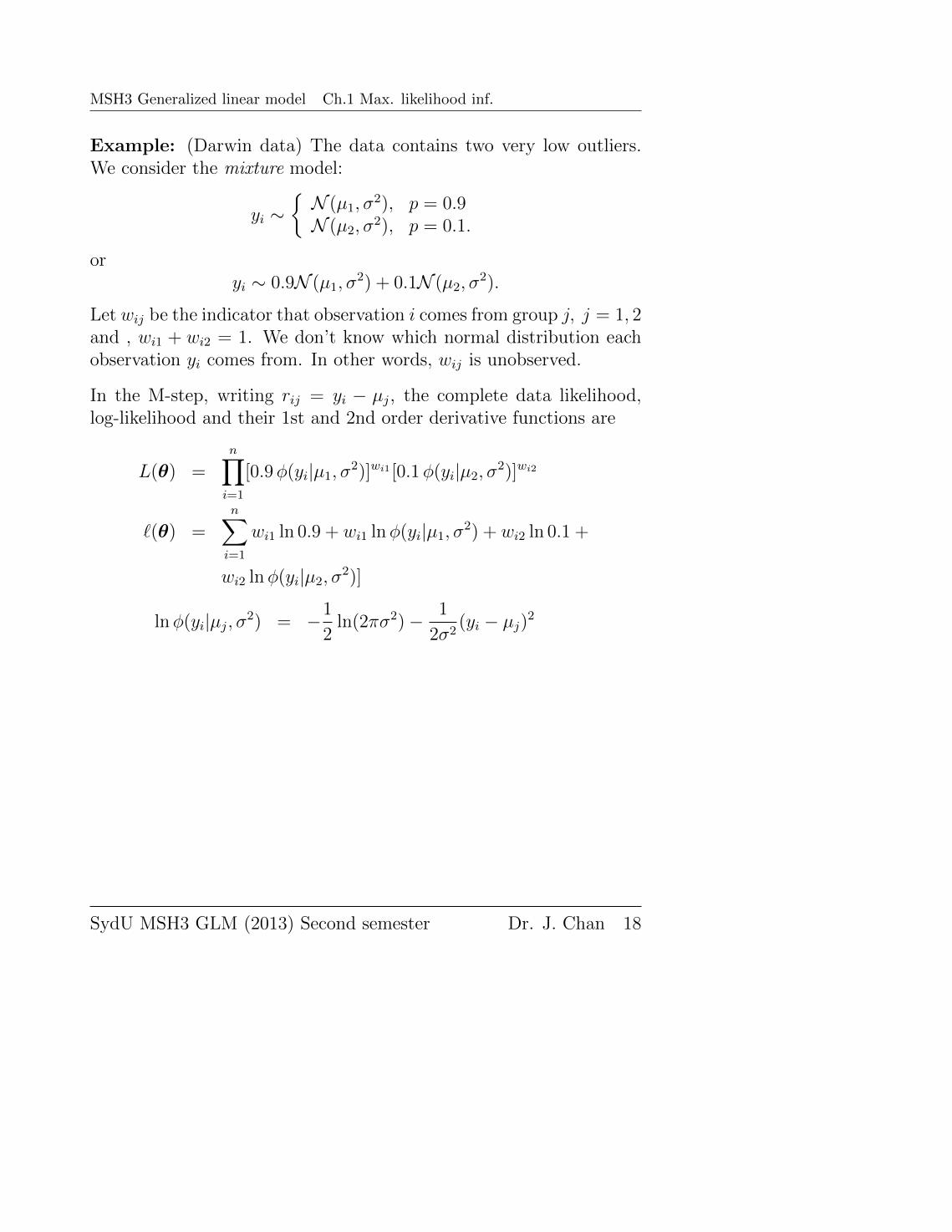
Example: (Darwin data) The data contains two very low outliers.We consider the mixture model:

yi ∼{N (µ1, σ

2), p = 0.9N (µ2, σ

2), p = 0.1.

oryi ∼ 0.9N (µ1, σ

2) + 0.1N (µ2, σ2).

Let wij be the indicator that observation i comes from group j, j = 1, 2and , wi1 + wi2 = 1. We don’t know which normal distribution eachobservation yi comes from. In other words, wij is unobserved.

In the M-step, writing rij = yi − µj, the complete data likelihood,log-likelihood and their 1st and 2nd order derivative functions are

L(θ) =n∏i=1

[0.9φ(yi|µ1, σ2)]wi1 [0.1φ(yi|µ2, σ

2)]wi2

`(θ) =n∑i=1

wi1 ln 0.9 + wi1 lnφ(yi|µ1, σ2) + wi2 ln 0.1 +

wi2 lnφ(yi|µ2, σ2)]

lnφ(yi|µj, σ2) = −1

2ln(2πσ2)− 1

2σ2(yi − µj)2

∂

∂µjlnφ(yi|µj, σ2) =

1

σ2(yi − µj) =

rijσ2

∂

∂σ2lnφ(yi|µj, σ2) = − 1

2σ2+

1

2σ4(yi − µj)2 =

1

2σ4(r2ij − σ2)

∂`(θ)

∂µj=

∂

∂µj

n∑i=1

wij lnφ(yi|µj, σ2) =1

σ2

n∑i=1

wijrij, j = 1, 2

∂`(θ)

∂σ2=

∂

∂σ2

n∑i=1

2∑j=1

wij lnφ(yi|µj, σ2) =1

2σ4

n∑i=1

2∑j=1

wij(r2ij − σ2)



∂`2(θ)

∂µ2j

=−1

σ2

n∑i=1

wij

∂`2(θ)

∂(σ2)2=−1

σ6

n∑i=1

2∑j=1

wij(r2ij − σ2)− n

2σ4

∂`2(θ)

∂µj∂σ2= − 1

σ4

n∑i=1

wijrij

∂`2(θ)

∂µ1∂µ2= 0

In the E-step, the conditional expectation of wi1 is

wi1 = 1 Pr(Wi1 = 1|yi) + 0 Pr(Wi1 = 0|yi) = Pr(Wi1 = 1|yi)

=Pr(Wi1 = 1, yi)

Pr(yi)=

Pr(Wi1 = 1) Pr(yi|Wi1 = 1)

Pr(yi)

=Pr(Wi1 = 1) Pr(yi|Wi1 = 1)

Pr(Wi1 = 1) Pr(yi|Wi1 = 1) + Pr(Wi1 = 0) Pr(yi|Wi1 = 0)

=0.9φ(yi|µ1, σ

2)

0.9φ(yi|µ1, σ2) + 0.1φ(yi|µ2, σ2)

> y=c(-67,-48,6,8,14,16,23,24,28,29,41,49,56,60,75)

> n=length(y)

> p=3 #no. of par.

> iterE=5

> iterM=10

> dim1=iterE*iterM

> dim2=2*p+3

> dl=c(rep(0,p))

> result=matrix(0,dim1,dim2)

> theta=c(30,-37,729) #starting values

>

> for (k in 1:iterE) { # E-step

+ ew1=0.9*exp(-0.5*(y-theta[1])^2/theta[3])

+ ew2=0.1*exp(-0.5*(y-theta[2])^2/theta[3])

+ w1=ew1/(ew1+ew2)

+ w1m=mean(w1)



+ w2=1-w1

+ sw1=sum(w1)

+ sw2=sum(w2)

+

+ for (i in 1:iterM) { # M-step

+ r1=y-theta[1]

+ r2=y-theta[2]

+ s1=r1^2-theta[3]

+ s2=r2^2-theta[3]

+ dl[1]=sum(w1*r1)/theta[3]

+ dl[2]=sum(w2*r2)/theta[3]

+ dl[3]=0.5*(sum(w1*s1)+sum(w2*s2))/theta[3]^2

+ dl2=matrix(0,p,p)

+ dl2[1,1]=-sw1/theta[3]

+ dl2[2,2]=-sw2/theta[3]

+ dl2[3,3]=-(sum(w1*s1)+sum(w2*s2))/theta[3]^3-0.5*n/theta[3]^2

+ dl2[3,1]=dl2[1,3]=-sum(w1*r1)/theta[3]^2

+ dl2[3,2]=dl2[2,3]=-sum(w2*r2)/theta[3]^2

+ dl2i=solve(dl2)

+ theta=theta-dl2i%*%dl

+ se=sqrt(diag(-dl2i))

+ l=log(0.9)*sw1+log(0.1)*sw2-n*log(2*pi*theta[3])/2

-(sum(w1*r1^2)+sum(w2*r2^2))/(2*theta[3])

+ row=(k-1)*10+i

+ result[row,]=c(k,i,theta[1],se[1],theta[2],se[2],theta[3],se[3],l)

+ }

+ }

> colnames(result)=c("iE","iM","mu1","se","mu2","se","sigma2","se","logL")

> result

iE iM mu1 se mu2 se sigma2 se logL

[1,] 1 1 33.48204 7.556567 -61.29223 20.36936 314.5368 333.38359 -74.72050

[2,] 1 2 32.67069 4.932458 -55.63190 12.80706 426.8732 92.08656 -75.11445

[3,] 1 3 32.28547 5.732025 -52.94443 14.65295 488.9407 144.09522 -74.00812

[4,] 1 4 32.22150 6.132491 -52.49817 15.64174 500.6744 176.38060 -73.88313

[5,] 1 5 32.21993 6.205593 -52.48720 15.82744 500.9943 182.76204 -73.88041

[6,] 1 6 32.21993 6.207575 -52.48719 15.83249 500.9945 182.93721 -73.88041

[7,] 1 7 32.21993 6.207576 -52.48719 15.83250 500.9945 182.93734 -73.88041

[8,] 1 8 32.21993 6.207576 -52.48719 15.83250 500.9945 182.93734 -73.88041

[9,] 1 9 32.21993 6.207576 -52.48719 15.83250 500.9945 182.93734 -73.88041

[10,] 1 10 32.21993 6.207576 -52.48719 15.83250 500.9945 182.93734 -73.88041

[11,] 2 1 33.13424 6.215236 -58.27681 15.93154 360.3297 207.03231 -72.33713

[12,] 2 2 32.95097 5.265502 -57.11632 13.42523 391.1934 125.81277 -72.12760

[13,] 2 3 32.93394 5.485894 -57.00847 13.98082 394.3075 142.27392 -72.09124

[14,] 2 4 32.93380 5.507683 -57.00761 14.03630 394.3344 143.97586 -72.09096

[15,] 2 5 32.93380 5.507870 -57.00761 14.03678 394.3344 143.99055 -72.09096

[16,] 2 6 32.93380 5.507870 -57.00761 14.03678 394.3344 143.99055 -72.09096

[17,] 2 7 32.93380 5.507870 -57.00761 14.03678 394.3344 143.99055 -72.09096



[18,] 2 8 32.93380 5.507870 -57.00761 14.03678 394.3344 143.99055 -72.09096

[19,] 2 9 32.93380 5.507870 -57.00761 14.03678 394.3344 143.99055 -72.09096

[20,] 2 10 32.93380 5.507870 -57.00761 14.03678 394.3344 143.99055 -72.09096

[21,] 3 1 32.99249 5.507838 -57.40463 14.03871 384.9492 145.69396 -71.91673

[22,] 3 2 32.99113 5.441860 -57.39541 13.86992 385.1901 140.51959 -71.91425

[23,] 3 3 32.99113 5.443563 -57.39540 13.87426 385.1903 140.65153 -71.91425

[24,] 3 4 32.99113 5.443564 -57.39540 13.87426 385.1903 140.65162 -71.91425

[25,] 3 5 32.99113 5.443564 -57.39540 13.87426 385.1903 140.65162 -71.91425

[26,] 3 6 32.99113 5.443564 -57.39540 13.87426 385.1903 140.65162 -71.91425

[27,] 3 7 32.99113 5.443564 -57.39540 13.87426 385.1903 140.65162 -71.91425

[28,] 3 8 32.99113 5.443564 -57.39540 13.87426 385.1903 140.65162 -71.91425

[29,] 3 9 32.99113 5.443564 -57.39540 13.87426 385.1903 140.65162 -71.91425

[30,] 3 10 32.99113 5.443564 -57.39540 13.87426 385.1903 140.65162 -71.91425

[31,] 4 1 32.99290 5.443541 -57.41186 13.87464 384.8527 140.71323 -71.90744

[32,] 4 2 32.99290 5.441156 -57.41185 13.86856 384.8531 140.52829 -71.90744

[33,] 4 3 32.99290 5.441158 -57.41185 13.86857 384.8531 140.52848 -71.90744

[34,] 4 4 32.99290 5.441158 -57.41185 13.86857 384.8531 140.52848 -71.90744

[35,] 4 5 32.99290 5.441158 -57.41185 13.86857 384.8531 140.52848 -71.90744

[36,] 4 6 32.99290 5.441158 -57.41185 13.86857 384.8531 140.52848 -71.90744

[37,] 4 7 32.99290 5.441158 -57.41185 13.86857 384.8531 140.52848 -71.90744

[38,] 4 8 32.99290 5.441158 -57.41185 13.86857 384.8531 140.52848 -71.90744

[39,] 4 9 32.99290 5.441158 -57.41185 13.86857 384.8531 140.52848 -71.90744

[40,] 4 10 32.99290 5.441158 -57.41185 13.86857 384.8531 140.52848 -71.90744

[41,] 5 1 32.99296 5.441157 -57.41245 13.86859 384.8414 140.53061 -71.90720

[42,] 5 2 32.99296 5.441074 -57.41245 13.86837 384.8414 140.52421 -71.90720

[43,] 5 3 32.99296 5.441074 -57.41245 13.86837 384.8414 140.52421 -71.90720

[44,] 5 4 32.99296 5.441074 -57.41245 13.86837 384.8414 140.52421 -71.90720

[45,] 5 5 32.99296 5.441074 -57.41245 13.86837 384.8414 140.52421 -71.90720

[46,] 5 6 32.99296 5.441074 -57.41245 13.86837 384.8414 140.52421 -71.90720

[47,] 5 7 32.99296 5.441074 -57.41245 13.86837 384.8414 140.52421 -71.90720

[48,] 5 8 32.99296 5.441074 -57.41245 13.86837 384.8414 140.52421 -71.90720

[49,] 5 9 32.99296 5.441074 -57.41245 13.86837 384.8414 140.52421 -71.90720

[50,] 5 10 32.99296 5.441074 -57.41245 13.86837 384.8414 140.52421 -71.90720

> w=cbind(w1,w2)

> w

w1 w2

[1,] 2.315067e-05 9.999768e-01

[2,] 2.004754e-03 9.979952e-01

[3,] 9.984605e-01 1.539495e-03

[4,] 9.990371e-01 9.629220e-04

[5,] 9.997646e-01 2.353932e-04

[6,] 9.998528e-01 1.471616e-04

[7,] 9.999716e-01 2.842587e-05

[8,] 9.999775e-01 2.247488e-05

[9,] 9.999912e-01 8.782696e-06

[10,] 9.999931e-01 6.944001e-06

[11,] 9.999996e-01 4.143677e-07

[12,] 9.999999e-01 6.327540e-08

[13,] 1.000000e+00 1.222089e-08

[14,] 1.000000e+00 4.775591e-09

[15,] 1.000000e+00 1.408457e-10

> mean(w1)

[1] 0.866605

From (wi1, wi2), the first two observations belong to group 2 while theothers all group 1. Hence EM method enables classification like clusteranalysis, an advantage over the classical likelihood method where themissing data wij are integrated out as the observed data likelihood

Lo(θ) =n∏i=1

[0.9φ(yi|µ1, σ2) + 0.1φ(yi|µ2, σ

2)] (8)



is a marginal mixture of two distributions and contains no missingobservations.

> x=rep(-0.001,n)

> x1=seq(-120,100,0.1)

> fx1=dnorm(x1,theta[1],sqrt(theta[3]))

> fx2=dnorm(x1,theta[2],sqrt(theta[3]))

> fx=0.9*fx1+0.1*fx2

> plot(x1, fx1, xlab="x", ylab="f(x)", ylim=c(-0.001,0.025),

xlim=c(-120,100), pch=20, col="red",cex=0.5)

> points(x1,fx2,pch=20,col=’blue’,cex=0.5)

> points(x1,fx,pch=20,cex=0.5)

> points(y,x,pch=20,cex=0.8)

> title("Mixture of normal distributions for Darwin data")

Note that this is a mixture model where the two model densities arerepresented by the blue and red lines. The mixed density in (8) isrepresented by the black line.



Example: (Right-Censored Data) with Darwin dataSuppose that the first four observations (ci, i = 1, . . . , 4) are rightcensored (yi > ci) and we assume that

zi, i = 1, . . . , 4; yi, i = 5, . . . , n ∼ N (µ, σ2).

Let θ = (µ, σ)′, z = (z1, . . . , z4) and y = (y5, . . . , yn). Then

`c(θ) = ln f(z,y|θ) = −n2

lnσ2 − 1

2σ2

4∑i=1

(zi − µ)2 − 1

2σ2

n∑i=5

(yi − µ)2

For the censored observations zi > ci, i = 1, . . . , 4, the conditionaldistribution is a truncated normal on (ci,∞), with the density function

f(z|µ, σ, ci) =φ(z|µ, σ2)

1− Φ(ci−µσ

) , z > ci (9)

where φ and Φ are the pdf and cdf functions for normal. Let θ(k) =(µ(k), σ2 (k)) be the current estimates of θ.

In the E-step, the conditional expectation of zi, i = 1, . . . , 4 given y,θ(k) and ci is

z(k)i = E(zi|y,θ(k), ci) =

∫ ∞ci

z f(z|µ(k), σ(k), ci) dz = µ(k) + σ(k)

∫ ∞c′i

tφ(t|0, 1)

1− Φ (c′i)dt

= µ(k) +φ(ci−µ(k)

σ(k)

)σ(k)

1− Φ(ci−µ(k)

σ(k)

)since for standardized normal variable ti = zi−µ(k)

σ(k) and c′i = ci−µ(k)

σ(k) ,

1√2π

∫ ∞c′

t exp

(−1

2t2)dt =

−1√2π

∫ ∞c′

exp

(−1

2t2)d

(−1

2t2)

=1√2π

exp

[−1

2(c′)2

]In the Monte Carlo approximation, the conditional expectation

z(k)i ' 1

S

S∑j=1

z(k)ij where z

(k)ij , j = 1, . . . , S is simulated from

f(z|µ(k), σ2 (k), ci) in (9) .



In the M-step, the z(k)i is substituted for the censored observation zi.

With the complete data (z(k),y), µ and σ2 of the normal data distri-bution are given by their sample mean and sample variance. Henceno iteration is required for the M-step.

> library("msm")

> cy=c(6,8,14,16,23,24,28,29,41,49,56,60,75) #first 4 obs are censored

> w=c(0,0,0,0,1,1,1,1,1,1,1,1,1)

> n=length(cy)

> S=10000 #sim 10000 z for z hat

> m=4 #first 4 censored

> p=2 #2 parmeters

> cen=cy[1:m] #censored obs

> y=cy[(m+1):n] #uncensored obs

> iterE=10

> dim=p+m+1

> result=matrix(0,iterE,dim)

> simz=matrix(0,m,S)

> z=rep(0,m)

> theta=c(mean(cy),var(cy)) #starting value for mu & sigma2

>

> for (k in 1:iterE) { #E-step

+

+ for (j in 1:m) {

+ # simz[j,]=rtnorm(S,mean=theta[1],sd=sqrt(theta[2]),lower=cen[j],

upper=Inf) #monte carlo approx. of E(Z|Z>c)

+ # z[j]=mean(simz[j,])

+

+ cz=(cen[j]-theta[1])/sqrt(theta[2])

+ z[j]=theta[1]+dnorm(cz)*sqrt(theta[2])/(1-pnorm(cz)) #exact

+ }

+ yr=c(z,y)

+ theta[1]=mean(yr) #M-step

+ theta[2]=(sum(yr^2)-sum(yr)^2/n)/n

+ result[k,]=c(k,theta[1],theta[2],z[1],z[2],z[3],z[4])

+

+ }

> colnames(result)=c("iE","mu","sigma2","ez1","ez2","ez3","ez4")

> print(result,digit=5) #monte carlo approx. of E(Z|Z>c)

iE mu sigma2 ez1 ez2 ez3 ez4



[1,] 1 41.630 211.67 37.262 37.842 40.054 41.036

[2,] 2 42.647 208.03 41.943 42.259 42.455 42.755

[3,] 3 42.921 208.09 42.540 43.007 43.614 43.810

[4,] 4 43.017 208.11 43.281 43.385 43.655 43.900

[5,] 5 43.040 208.17 43.154 43.441 43.733 44.188

[6,] 6 43.048 208.21 42.985 43.371 44.071 44.201

[7,] 7 43.046 208.18 43.158 43.473 43.689 44.277

[8,] 8 43.036 208.14 43.393 43.317 43.721 44.039

[9,] 9 43.061 208.19 43.375 43.298 43.968 44.156

[10,] 10 43.071 208.22 43.336 43.364 43.810 44.411

> print(result,digit=5) #exact E(Z|Z>c)

iE mu sigma2 ez1 ez2 ez3 ez4

[1,] 1 41.659 211.47 37.377 37.996 40.180 41.018

[2,] 2 42.660 208.05 41.948 42.062 42.638 42.932

[3,] 3 42.930 208.06 42.889 42.983 43.478 43.737

[4,] 4 43.006 208.12 43.148 43.239 43.718 43.969

[5,] 5 43.027 208.14 43.221 43.311 43.785 44.035

[6,] 6 43.033 208.15 43.242 43.332 43.805 44.054

[7,] 7 43.035 208.15 43.248 43.337 43.810 44.059

[8,] 8 43.035 208.15 43.249 43.339 43.812 44.061

[9,] 9 43.036 208.15 43.250 43.339 43.812 44.061

[10,] 10 43.036 208.15 43.250 43.340 43.812 44.061

The convergence using Monte Carlo approx. is subjected to randomerror in the simulation. Parameter estimates are given by the averagesover iterations.



§1.6.2 Monte Carlo EM Algorithm

Given the current guess to the posterior mode, θ(k), the conditional ex-pectation in the E-step may involve integration and can be calculatedusing Monte Carlo (MC) approximation. Similarly the complete datalog-likelihood function `c(θ) = ln f(y, z|θ) can also be approximatedusing MC approximation:

ˆc(θ) = ln f(y, z|θ) =

1

S

S∑j=1

ln f(y, z(k)j |θ) (10)

where z(k)1 , . . . ,z

(k)S ∼ f(z|θ(k),y) as required in the E-step. This

maximizes an average of log-likelihood ln f(y, z|θ) based on simulatedvalues which is different from maximizing ln f(y, z|θ) where z is theaverage of simulated values. Then, in the M-step, we maximize ˆ

c(θ)in (10) to obtain a new guess, θ(k+1).Monitoring the convergence: Plot each component of θ(k) against theiteration number k.

Example: (Right-Censored Data) Consider the Darwin data again.In the E-step, the conditional expectation of zi given y, θ(k) and ci isestimated by drawing sample z

(k)i1 , z

(k)i2 , . . . , z

(k)iS from the truncated nor-

mal f(zi|µ(k), σ(k), ci) in (9) at the current estimates θ(k) = (µ(k), σ(k)).

In the M-step, one obtains a MC approximation to ln f(y, z|θ) by

ˆc(θ) =

1

S

S∑j=1

[−n

2ln(2πσ2)− 1

2σ2

4∑i=1

(z(k)ij − µ)2 +

n∑i=5

(yi − µ)2

]

= −n2

ln(2πσ2)− 1

2σ2

[4∑i=1

(1

S

S∑j=1

(z(k)ij − µ)2

)+

n∑i=5

(yi − µ)2

]

and maximizes it w.r.t. θ to obtain θ(k+1) through iterations insteadof close-form solution. Write ri = yi − µ, i = 5, . . . , n, rij = z

(k)ij − µ,



zi = 1S

S∑j=1

z(k)ij and ri = zi − µ, i = 1, . . . , 4,

∂ ˆ(θ)

∂µ=

1

σ2

4∑i=1

1

S

S∑j=1

(z(k)it − µ)

+

n∑i=5

(yi − µ)

=1

σ2

n∑i=1

ri,

∂ ˆ(θ)

∂σ2=

1

2σ4

4∑i=1

1

S

S∑j=1

(z(k)ij − µ)2

+

n∑i=5

(yi − µ)2 − nσ2

=

1

2σ4

4∑i=1

1

S

S∑j=1

r2ij

− σ2

+

n∑i=5

(r2i − σ2)

Since

1

S

S∑j=1

r2ij =1

S

S∑j=1

(z(k)it − µ)2 6=

1

S

S∑j=1

(z(k)it − µ)

2

=

1

S

S∑j=1

rij

2

= r2i ,

closed-form solution using sample mean and sample variance can not be used.

∂ ˆ2(θ)

∂µ2=−nσ2

∂ ˆ2(θ)

∂(σ2)2=−1

σ6

4∑i=1

1

S

S∑j=1

(z(k)ij − µ)2

+n∑i=5

(yi − µ)2

+n

2σ4

=−1

σ6

4∑i=1

1

S

S∑j=1

r2ij

− σ2

+

n∑i=5

(r2i − σ2)

− n

2σ4

∂ ˆ2(θ)

∂µ∂σ2= − 1

σ4

n∑i=1

ri

> library("msm")

> cy=c(6,8,14,16,23,24,28,29,41,49,56,60,75) #first 4 obs are censor time

> w=c(0,0,0,0,1,1,1,1,1,1,1,1,1)

> mean(cy)

[1] 33

> n=length(cy)

> T=10000 #sim 10000 z for z hat

> m=4 #first 4 censored obs

> p=2 #2 pars



> cen=cy[1:m] #censored obs

> y=cy[(m+1):n] #uncensored obs

> iterE=5

> iterM=10

> dim1=iterE*iterM

> dim2=2*p+7

> dl=c(rep(0,p))

> dl2=matrix(0,p,p)


> simz=matrix(0,m,T)

> z=matrix(0,m,1)

> rz=rep(0,m)

> r2z=rep(0,m)

> theta=c(40,400) #starting values for mu & var

>

> for (k in 1:iterE) { #E-step

+ for (j in 1:m) {

+ simz[j,]=rtnorm(T,mean=theta[1],sd=sqrt(theta[2]),lower=cen[j],

upper=Inf)

+ z[j]=mean(simz[j,])

+ }

+

+ for (i in 1:iterM) { #M-step

+ rz=z-theta[1]

+ ry=y-theta[1]

+ r=c(rz,ry)

+ r2z=apply((simz-theta[1])^2,1,mean)

+ r2=c(r2z,ry^2)

+ s2=r2-theta[2]

+ dl[1]=sum(r)/theta[2]

+ dl[2]=0.5*sum(s2)/theta[2]^2

+ dl2[1,1]=-n/theta[2]

+ dl2[2,2]=-sum(s2)/theta[2]^3-0.5*n/theta[2]^2

+ dl2[2,1]=dl2[1,2]=-sum(r)/theta[2]^2

+ dl2i=solve(dl2)

+ theta=theta-dl2i%*%dl

+ se=sqrt(diag(-dl2i))

+ l=-n*log(2*pi*theta[2])/2-sum(r^2)/(2*theta[2]) #pi=3.141593

+ row=(k-1)*10+i

+ result[row,]=c(k,i,theta[1],se[1],theta[2],se[2],l,z[1],z[2],



z[3],z[4])

+ }

+ }

> colnames(result)=c("iE","iM","mu","se","sigma2","se","logL","ez1",

"ez2","ez3","ez4")

> print(result,digit=5)

iE iM mu se sigma2 se logL ez1 ez2 ez3 ez4

[1,] 1 1 43.745 5.6699 288.50 160.37 -53.653 42.163 42.427 44.008 44.473

[2,] 1 2 42.965 4.7218 301.25 113.42 -53.557 42.163 42.427 44.008 44.473

[3,] 1 3 42.929 4.8139 301.86 118.16 -53.547 42.163 42.427 44.008 44.473

[4,] 1 4 42.929 4.8187 301.86 118.40 -53.547 42.163 42.427 44.008 44.473

[5,] 1 5 42.929 4.8187 301.86 118.40 -53.547 42.163 42.427 44.008 44.473

[6,] 1 6 42.929 4.8187 301.86 118.40 -53.547 42.163 42.427 44.008 44.473

[7,] 1 7 42.929 4.8187 301.86 118.40 -53.547 42.163 42.427 44.008 44.473

[8,] 1 8 42.929 4.8187 301.86 118.40 -53.547 42.163 42.427 44.008 44.473

[9,] 1 9 42.929 4.8187 301.86 118.40 -53.547 42.163 42.427 44.008 44.473

[10,] 1 10 42.929 4.8187 301.86 118.40 -53.547 42.163 42.427 44.008 44.473

[11,] 2 1 43.280 4.8205 287.03 118.44 -53.460 43.734 43.914 44.876 44.900

[12,] 2 2 43.263 4.6989 287.16 112.58 -53.458 43.734 43.914 44.876 44.900

[13,] 2 3 43.263 4.6999 287.16 112.63 -53.458 43.734 43.914 44.876 44.900

[14,] 2 4 43.263 4.6999 287.16 112.63 -53.458 43.734 43.914 44.876 44.900

[15,] 2 5 43.263 4.6999 287.16 112.63 -53.458 43.734 43.914 44.876 44.900

[16,] 2 6 43.263 4.6999 287.16 112.63 -53.458 43.734 43.914 44.876 44.900

[17,] 2 7 43.263 4.6999 287.16 112.63 -53.458 43.734 43.914 44.876 44.900

[18,] 2 8 43.263 4.6999 287.16 112.63 -53.458 43.734 43.914 44.876 44.900

[19,] 2 9 43.263 4.6999 287.16 112.63 -53.458 43.734 43.914 44.876 44.900

[20,] 2 10 43.263 4.6999 287.16 112.63 -53.458 43.734 43.914 44.876 44.900

[21,] 3 1 43.320 4.6999 284.71 112.63 -53.446 44.105 43.867 44.783 45.399

[22,] 3 2 43.320 4.6799 284.72 111.67 -53.446 44.105 43.867 44.783 45.399

[23,] 3 3 43.320 4.6799 284.72 111.68 -53.446 44.105 43.867 44.783 45.399

[24,] 3 4 43.320 4.6799 284.72 111.68 -53.446 44.105 43.867 44.783 45.399

[25,] 3 5 43.320 4.6799 284.72 111.68 -53.446 44.105 43.867 44.783 45.399

[26,] 3 6 43.320 4.6799 284.72 111.68 -53.446 44.105 43.867 44.783 45.399

[27,] 3 7 43.320 4.6799 284.72 111.68 -53.446 44.105 43.867 44.783 45.399

[28,] 3 8 43.320 4.6799 284.72 111.68 -53.446 44.105 43.867 44.783 45.399

[29,] 3 9 43.320 4.6799 284.72 111.68 -53.446 44.105 43.867 44.783 45.399

[30,] 3 10 43.320 4.6799 284.72 111.68 -53.446 44.105 43.867 44.783 45.399

[31,] 4 1 43.325 4.6799 284.61 111.68 -53.446 43.945 43.878 45.109 45.295

[32,] 4 2 43.325 4.6790 284.61 111.63 -53.446 43.945 43.878 45.109 45.295

[33,] 4 3 43.325 4.6790 284.61 111.63 -53.446 43.945 43.878 45.109 45.295

[34,] 4 4 43.325 4.6790 284.61 111.63 -53.446 43.945 43.878 45.109 45.295

[35,] 4 5 43.325 4.6790 284.61 111.63 -53.446 43.945 43.878 45.109 45.295

[36,] 4 6 43.325 4.6790 284.61 111.63 -53.446 43.945 43.878 45.109 45.295

[37,] 4 7 43.325 4.6790 284.61 111.63 -53.446 43.945 43.878 45.109 45.295

[38,] 4 8 43.325 4.6790 284.61 111.63 -53.446 43.945 43.878 45.109 45.295

[39,] 4 9 43.325 4.6790 284.61 111.63 -53.446 43.945 43.878 45.109 45.295

[40,] 4 10 43.325 4.6790 284.61 111.63 -53.446 43.945 43.878 45.109 45.295

[41,] 5 1 43.343 4.6790 284.06 111.63 -53.443 44.072 44.284 44.957 45.149

[42,] 5 2 43.343 4.6745 284.06 111.42 -53.443 44.072 44.284 44.957 45.149

[43,] 5 3 43.343 4.6745 284.06 111.42 -53.443 44.072 44.284 44.957 45.149

[44,] 5 4 43.343 4.6745 284.06 111.42 -53.443 44.072 44.284 44.957 45.149

[45,] 5 5 43.343 4.6745 284.06 111.42 -53.443 44.072 44.284 44.957 45.149

[46,] 5 6 43.343 4.6745 284.06 111.42 -53.443 44.072 44.284 44.957 45.149

[47,] 5 7 43.343 4.6745 284.06 111.42 -53.443 44.072 44.284 44.957 45.149

[48,] 5 8 43.343 4.6745 284.06 111.42 -53.443 44.072 44.284 44.957 45.149

[49,] 5 9 43.343 4.6745 284.06 111.42 -53.443 44.072 44.284 44.957 45.149

[50,] 5 10 43.343 4.6745 284.06 111.42 -53.443 44.072 44.284 44.957 45.149



§1.6.3 Expectation Conditional Maximization (ECM) algo-rithm

What if the M-step is computationally intensive?Meng and Rubin (1993) suggested to replace the complicated M-stepwith several computationally simple conditional maximization stepsand developed the Expectation Conditional Maximization (ECM) al-gorithm.

Let θ = (θ1, . . . , θp)′.

The M-steps of the ECM algorithm are proceeded as follows:

Maximize f(y|z∗k,θ) w.r.t. θ1, to obtain θk+11 , keeping θ2 = θk2 , . . . , θp = θkp .

Maximize f(y|z∗k,θ) w.r.t. θ2, to obtain θk+12 , keeping θ1 = θk+1

1 , θ3 = θk3 , . . . , θp−1 =θkp−1....

Maximize f(y|z∗k,θ) w.r.t. θp, to obtain θk+1p , keeping θ1 = θk+1

1 , . . . , θp = θk+1p .

Hence θk+1 = (θk+11 , . . . , θk+1

p ) is a new guess of the posterior mode.For further details about ECM, see Meng & Rubin (1993, 1994) andLiu & Rubin (1994, 1995).

Motivating example: Suppose Yi ∼ tν(µ, σ2). Using the scale mix-

ture of normals (SMN) representing of Student-t distribution, we have

Yi ∼ N(µ,σ2

λi

), λi ∼ G

(ν2,ν

2

),

or equivalently,

ft(yi|µ, σ2, ν) =

∫ ∞0

fN

(yi

∣∣∣µ, σ2

λi

)fG

(λi

∣∣∣ν2,ν

2

)dλ (11)

where ft(·|µ, σ2, ν) is the pdf of t distribution, fN(·|µ, σ2) is the pdf ofnormal distribution and fG(·|a, b) is the pdf of gamma distribution ofthe form

fG(λ|a, b) =ba

Γ(a)λa−1e−bλ, λ, a, b > 0



with E(λ) = ab, E(log λ) = ψ(a)+log(b) and ψ(x) = ∂

∂xln Γ(x) = Γ′(x)

Γ(x)

is a digamma function.

Condition on the mixing or state parameter λi, Yi follow a normaldistribution where µ is estimated by sample mean and σ2 by samplevariance. The mixing parameter λi can be used to detect outliers (if1λi> 2.5 say).

E-step for λi: To find the conditional expectation, it is easy to seethat the conditional density of f(λi|yi) is given by

λi|yi ∼ G(ν + 1

2,ν + y2

i

2

).

To show this, it is sufficient to find the functional form of the condi-tional density.

f(λi|yi) ∝ f(λi, yi)

∝√λi exp

(−λi

2z2i

)λν2−1

i exp(−ν

2λi

)∝ λ

ν2

+ 12−1

i exp

[−λi

2

(z2i + ν

)]∼ G

(ν + 1

2,ν + z2

i

2

).

where zi = yi−µσ

. Thus

E [λi|yi] =ν + 1

ν + z2i

, (12)

E [log λi|yi] = ψ

(ν + 1

2

)− log

(ν + z2

i

2

). (13)

(14)

CM-step for µ and σ:



Since the conditional distribution of Yi|λi is N (µ, σ2/λi), the condi-tional likelihood and loglikelihood are

L =n∏i=1

√λi√

2πσ2exp

[− λi

2σ2(yi − µ)2

],

`N =− n

2log 2π − n

2log σ2 +

1

2

n∑i=1

log λi −1

2σ2

n∑i=1

λi(yi − µ)2,

and the first derivatives are:

∂`N∂µ

= − 1

2σ2

n∑i=1

λi(yi − µ) · −2 =1

σ2

n∑i=1

λi(yi − µ)

∂`N∂σ2

= − n

2σ2− −1

2σ4

n∑i=1

λi(yi − µ)2 =1

2σ2

(−n+

1

σ2

n∑i=1

λi(yi − µ)2

).

Setting∂`

∂µ= 0 and

∂`

∂σ2= 0, we have

1

σ2

n∑i=1

λi(yi − µ) = 0 ⇒ µ =

n∑i=1

λiyi

n∑i=1

λi

−n+1

σ2

n∑i=1

λi(yi − µ)2 = 0 ⇒ σ2 =1

n

n∑i=1

λi(yi − µ)2

CM-step for ν:Since λi follows G(ν

2, ν

2), the conditional likelihood and loglikelihood

are given by

L =n∏i=1

(ν2

) ν2

Γ(ν2

)λ ν2−1

i exp(−ν

2λi

),

` =nν

2log(ν

2

)− n log Γ

(ν2

)+(ν

2− 1) n∑i=1

log λi −ν

2

n∑i=1

λi



and the first and second order derivatives are:

∂`

∂ν=

n

2log(ν

2

)+n

2− n

2ψ(ν

2

)+

1

2

n∑i=1

(log λi − λi),

∂2`

∂ν2=

n

2

[1

ν− 1

2ψ′(ν

2

)].

where estimates of λi and log λi are given by E(λi) and E(log λi) in(12) and (13) respectively. Then NR algorithm can be used to solve for∂`

∂ν= 0. If one more expectation is inserted between the estimation of

(µ, σ2) and ν, the method is called MCECM. Furthermore, if the truelikelihood using t instead of gamma distributions is adopted for theestimation of ν, the method is called ECME. In this case, the actuallog-likelihood and their derivatives are

` ∝ n log Γ

(ν

2+

1

2

)− n

2log ν − n log Γ

(ν2

)− ν + 1

2

n∑i=1

log

(1 +

z2iν

)∂`

∂ν=

n

2ψ

(1

2+ν

2

)− n

2ψ(ν

2

)− n

2ν− 1

2

n∑i=1

log

(1 +

z2iν

)+ν + 1

2ν2

n∑i=i

z2i

1 +z2iν

∂2`

∂ν2=

n

2ν2+ν + 1

2ν4

n∑i=i

z4i(1 +

z2iν

)2 − 1

ν3

n∑i=i

z2i

1 +z2iν

+n

4ψ′(

1

2+ν

2

)− n

4ψ′(ν

2

)

Example (Darwin data) The R program for fitting a t distributionto the data using the MCECM and ECME methods is

> y=c(-67,-48,6,8,14,16,23,24,28,29,41,49,56,60,75)

> n=length(y)

> p=3 #no. of par

> iterE = 1000

> iterM = 20

> dim1=iterE

> dim2=p+3


> tol=1E-7



>

> ECM.method="MCECM"

> mu=mean(y) #starting values

> sig2=var(y)

> df=5

>

> #### start ECM algorithm #####

>

> for (k in 1:iterE) {

+

+ ### E-step ###

+ z2={y-mu}^2/sig2

+ elam={df+1}/{z2+df}

+

+ slamy <- sum(y*elam)

+ slam <- sum(elam)

+

+ ### CM-step 1 ###

+ mu=slamy/slam

+ sig2=sum(elam*{y-mu}^2)/n

+

+ ### E-step ###

+ z2={y-mu}^2/sig2

+ elam={df+1}/{z2+df}

+ eloglam=digamma({df+1}/2) - log({df+z2}/2)

+

+ slam=sum(elam)

+ sloglam=sum(eloglam)

+

+ ### CM-step2 ###using Newton Rapson method

+ if (ECM.method == "MCECM"){

+

+ for (i in 1:iterM) {

+ dl=n/2*{log(df/2) + 1 - digamma(df/2)} + 0.5*{sloglam - slam}

+ dl2=n/2*{1/df - 0.5*trigamma(df/2)}

+ df=df - dl/dl2

+

+ }

+ }

+



+ if (ECM.method == "ECME"){

+

+ for (i in 1:iterM) {

+ dl=n/2*{digamma({1+df}/2)-digamma(df/2)-1/df}-0.5*sum(log(1+z2/df))

+{1+df}/2/df^2*sum(z2/{1+z2/df})

+ dl2=n/4*{2/df^2+trigamma({1+df}/2)-trigamma(df/2)}+{df+1}/2/df^4*

sum(z2^2/{1+z2/df}^2)-1/df^3*sum(z2/{1+z2/df})

+ df=df-dl/dl2

+ }

+ }

+

+ l=n*{lgamma(df/2+0.5)-lgamma(df/2)-log(pi*df*sig2)/2}

-{df/2+0.5}*sum(log(1+z2/df))

+ result[k,]=c(k,i,mu,sig2,df,l)

+

+ if (k > 1){if(max(abs(result[k,3:{2+p}]-result[k-1,3:{2+p}])) < tol) break}

+

+ }

>

> colnames(result) <- c("iE","iM","mu","sigma2","df","logL");

> print(result[1:k,])

iE iM mu sigma2 df logL #MCECM

[1,] 1 20 24.13682 997.6178 5.059856 -74.88605

[2,] 2 20 25.22351 866.2626 4.961330 -74.76863

[3,] 3 20 25.67029 810.3751 4.801414 -74.73389

[4,] 4 20 25.89719 779.6043 4.623208 -74.71350

[5,] 5 20 26.04214 758.1033 4.444446 -74.69631

[6,] 6 20 26.15324 740.2754 4.272297 -74.68035

[7,] 7 20 26.24766 724.0743 4.109642 -74.66528

[8,] 8 20 26.33155 708.7673 3.957593 -74.65111

[9,] 9 20 26.40703 694.1197 3.816490 -74.63790

[10,] 10 20 26.47483 680.0846 3.686292 -74.62574

...

[171,] 171 20 26.83978 515.0666 2.500910 -74.54620

[172,] 172 20 26.83978 515.0666 2.500910 -74.54620

[173,] 173 20 26.83978 515.0666 2.500910 -74.54620

[174,] 174 20 26.83978 515.0666 2.500910 -74.54620

[175,] 175 20 26.83978 515.0666 2.500910 -74.54620

> elam

[1] 0.1786403 0.2617460 1.0468932 1.0974573 1.2410240 1.2828370 1.3840132

[8] 1.3911453 1.3983932 1.3948015 1.2113025 1.0134842 0.8432270 0.7551933

[15] 0.4998422

> iE iM mu sigma2 df logL #ECME

[1,] 1 20 24.13682 997.6178 5.618581 -74.88150

[2,] 2 20 25.07158 887.6227 4.504478 -74.77776

[3,] 3 20 25.72984 799.4537 3.863545 -74.69887

[4,] 4 20 26.16745 731.3709 3.463950 -74.64377

[5,] 5 20 26.44556 679.7935 3.200413 -74.60741

[6,] 6 20 26.61652 640.9790 3.019233 -74.58423

[7,] 7 20 26.71890 611.7496 2.890701 -74.56971



[8,] 8 20 26.77875 589.6431 2.797309 -74.56072

[9,] 9 20 26.81283 572.8284 2.728192 -74.55516

[10,] 10 20 26.83156 559.9637 2.676312 -74.55174

...

[84,] 84 20 26.83978 515.0666 2.500910 -74.54620

[85,] 85 20 26.83978 515.0666 2.500910 -74.54620

[86,] 86 20 26.83978 515.0666 2.500910 -74.54620

[87,] 87 20 26.83978 515.0666 2.500910 -74.54620

[88,] 88 20 26.83978 515.0666 2.500910 -74.54620

[89,] 89 20 26.83978 515.0666 2.500910 -74.54620

The first two observations are identified as outliers since1λi

= 10.1786

= 5.5978 or 1/0.2617 = 3.8205.

References

Dempster, A.P., Laird, N. & Rubin, D.B. (1977) Maximum likelihood from incom-plete data via the EM algorithm. Journal of the Royal Statistical Society,Series B, 39, 1-38. (with discussion).

McLachlan, G.J. & Krishnan, T (1997) The EM Algorithm and Extensions. Wi-ley.



where in the diagram, θ(k+1) ≡ θ, θn+1, `∗o(θ(k+1)|θ(k)) ≡ `(θ|θn) and

ò(θ(k+1)) ≡ L(θn+1). The function `∗o(θ|θ(k)) is bounded above by

the log-likelihood function ò(θ).

Next we show (ii) that `∗o(θ|θ(k)) and ò(θ) are equal at θ = θ(k).

`∗o(θ(k)|θ(k)) = ò(θ

(k)) + ∆(θ(k)|θ(k))

= ò(θ(k)) +

∫ ∞−∞

f(z|y,θ(k)) lnf(y|z,θ(k))f(z|θ(k))

f(z|y,θ(k))f(y|θ(k))dz

= ò(θ(k)) +

∫ ∞−∞

f(z|y,θ(k)) lnf(y, z|θ(k))

f(y, z|θ(k))dz

= ò(θ(k)).

Hence any θ(k+1) which increases `∗o(θ(k+1)|θ(k)) also increases ò(θ

(k+1)).

Lastly, we show (iii) that the EM algorithm chooses θ(k+1) for which`∗o(θ|θ(k)) is a maximum. Since ò(θ) ≥ `∗o(θ|θ(k)), increasing `∗o(θ|θ(k))ensures that ò(θ) is increased at each step.

To achieve the greatest increase in ò(θ(k+1)), EM algorithm selects

θ(k+1) which maximize `∗o(θ|θ(k)), i.e.

θ(k+1) = arg maxθ

[`∗o(θ|θ(k))] = arg maxθ

[ò(θ(k)) + ∆(θ|θ(k))]

= arg maxθ

[ò(θ

(k)) +

∫ ∞−∞

f(z|y,θ(k)) lnf(y|z,θ)f(z|θ)

f(z|y,θ(k))f(y|θ(k))dz

]= arg max

θ

[∫ ∞−∞

f(z|y,θ(k)) ln[f(y|z,θ)f(z|θ)] dz

](drop the constant term w.r.t. θ)

= arg maxθ

[∫ ∞−∞

ln f(y, z|θ)f(z|y,θ(k)) dz]

= arg maxθ

[Ez|y,θ(k){ln f(y, z|θ)}

]and hence proved (7).


MSH3 Generalized Linear model (Part 1) · MSH3 Generalized Linear model (Part 1) Jennifer S.K. CHAN...

Documents

Transcript of MSH3 Generalized Linear model (Part 1) · MSH3 Generalized Linear model (Part 1) Jennifer S.K. CHAN...