Introduction to Generalized Linear Models · Generalized linear models extend the general linear...

Introduction to Generalized Linear Models

Heather Turner

ESRC National Centre for Research Methods, UKand

Department of StatisticsUniversity of Warwick, UK

WU, 2008–04–22-24

Copyright c© Heather Turner, 2008


Introduction

This short course provides an overview of generalized linear models(GLMs).

We shall see that these models extend the linear modellingframework to variables that are not Normally distributed.

GLMs are most commonly used to model binary or count data, sowe will focus on models for these types of data.


Outlines

Plan

Part I: Introduction to Generalized Linear Models

Part II: Binary Data

Part III: Count Data


Outlines

Part I: Introduction to Generalized Linear Models

Part I: Introduction

Review of Linear Models

Generalized Linear Models

GLMs in R

Exercises


Outlines



Binary Data

Models for Binary Data

Model Selection

Model Evaluation

Exercises


Outlines



Count Data

Modelling Rates

Modelling Contingency Tables

Exercises

Introduction

Part I


Introduction


Structure

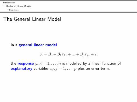
The General Linear Model

In a general linear model

yi = β0 + β1x1i + ...+ βpxpi + εi

the response yi, i = 1, . . . , n is modelled by a linear function ofexplanatory variables xj , j = 1, . . . , p plus an error term.

Introduction


Structure

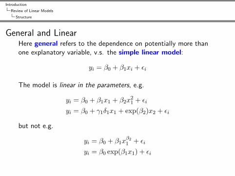
General and LinearHere general refers to the dependence on potentially more thanone explanatory variable, v.s. the simple linear model:

yi = β0 + β1xi + εi

The model is linear in the parameters, e.g.

yi = β0 + β1x1 + β2x21 + εi

yi = β0 + γ1δ1x1 + exp(β2)x2 + εi

but not e.g.

yi = β0 + β1xβ21 + εi

yi = β0 exp(β1x1) + εi

Introduction


Structure

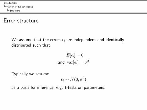
Error structure

We assume that the errors εi are independent and identicallydistributed such that

E[εi] = 0

and var[εi] = σ2

Typically we assumeεi ∼ N(0, σ2)

as a basis for inference, e.g. t-tests on parameters.

Introduction


Examples

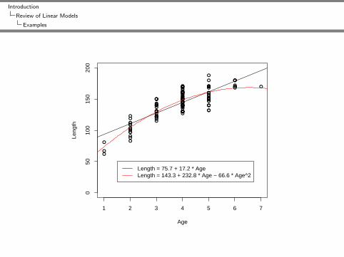
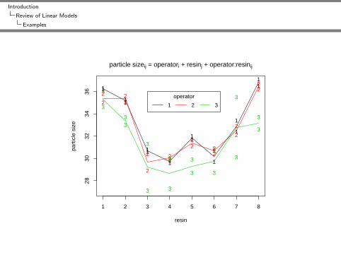
Some Examples

abdomin

6080100120140160

biceps

2530

3540

45

bodyfat

0

20

40

60

bodyfat = −14.59 + 0.7 * biceps − 0.9 * abdomin

Introduction


Examples

●●

●

●

●●

●●

●●●●

●

●●

● ●

●●

●●●●●●

●●●●●●●●●●●● ●

●

●●

●

●

●

●

●

●

●

●●

●●

●

●● ●

●

●

●

●

● ●●●● ●

●

●

●

●

●

●

● ●

●

●

●

●

●

●

●

●●

●

●

●

●

●

●

●●

●

●

●

●

●

●

●

●

●●

●

●

●●●●●

●●

●●●● ●

●●●●● ●●

●●●●●

●● ●●● ●●

●

●

●

●

●●

1 2 3 4 5 6 7

050

100

150

200

Age

Leng

th

Length = 75.7 + 17.2 * AgeLength = 143.3 + 232.8 * Age − 66.6 * Age^2

Introduction


Examples

1 2 3 4 5 6 7 8

2830

3234

36

particle sizeij = operatori + resinj + operator:resinij

resin

part

icle

siz

e

11

11

11

11

11

1

1

1

1

11

2

222

2

2

22

22

22

2

2

223

3

33

3

3

3

3

3

3

3

3

3

3

3

3

operator

1 2 3

Introduction


Restrictions

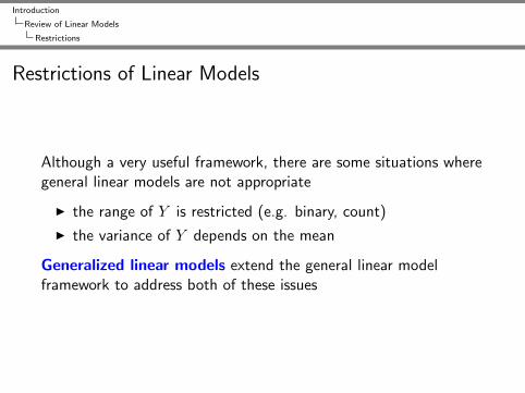
Restrictions of Linear Models

Although a very useful framework, there are some situations wheregeneral linear models are not appropriate

I the range of Y is restricted (e.g. binary, count)

I the variance of Y depends on the mean

Generalized linear models extend the general linear modelframework to address both of these issues

Introduction


Structure

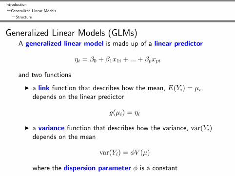
Generalized Linear Models (GLMs)A generalized linear model is made up of a linear predictor

ηi = β0 + β1x1i + ...+ βpxpi

and two functions

I a link function that describes how the mean, E(Yi) = µi,depends on the linear predictor

g(µi) = ηi

I a variance function that describes how the variance, var(Yi)depends on the mean

var(Yi) = φV (µ)

where the dispersion parameter φ is a constant

Introduction


Structure

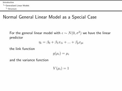
Normal General Linear Model as a Special Case

For the general linear model with ε ∼ N(0, σ2) we have the linearpredictor

ηi = β0 + β1x1i + ...+ βpxpi

the link functiong(µi) = µi

and the variance function

V (µi) = 1

Introduction


Structure

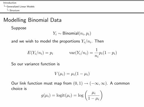
Modelling Binomial Data

SupposeYi ∼ Binomial(ni, pi)

and we wish to model the proportions Yi/ni. Then

E(Yi/ni) = pi var(Yi/ni) =1nipi(1− pi)

So our variance function is

V (µi) = µi(1− µi)

Our link function must map from (0, 1)→ (−∞,∞). A commonchoice is

g(µi) = logit(µi) = log(

µi1− µi

)

Introduction


Structure

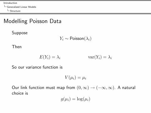
Modelling Poisson Data

SupposeYi ∼ Poisson(λi)

Then

E(Yi) = λi var(Yi) = λi

So our variance function is

V (µi) = µi

Our link function must map from (0,∞)→ (−∞,∞). A naturalchoice is

g(µi) = log(µi)

Introduction


Structure

Transformation vs. GLM

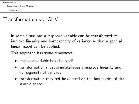
In some situations a response variable can be transformed toimprove linearity and homogeneity of variance so that a generallinear model can be applied.

This approach has some drawbacks

I response variable has changed!

I transformation must simulateneously improve linearity andhomogeneity of variance

I transformation may not be defined on the boundaries of thesample space

Introduction


Structure

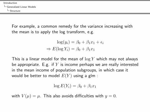
For example, a common remedy for the variance increasing withthe mean is to apply the log transform, e.g.

log(yi) = β0 + β1x1 + εi

⇒ E(log Yi) = β0 + β1x1

This is a linear model for the mean of log Y which may not alwaysbe appropriate. E.g. if Y is income perhaps we are really interestedin the mean income of population subgroups, in which case itwould be better to model E(Y ) using a glm :

logE(Yi) = β0 + β1x1

with V (µ) = µ. This also avoids difficulties with y = 0.

Introduction


Structure

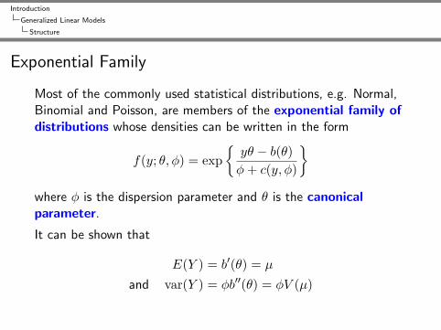
Exponential Family

Most of the commonly used statistical distributions, e.g. Normal,Binomial and Poisson, are members of the exponential family ofdistributions whose densities can be written in the form

f(y; θ, φ) = exp{yθ − b(θ)φ+ c(y, φ)

}where φ is the dispersion parameter and θ is the canonicalparameter.

It can be shown that

E(Y ) = b′(θ) = µ

and var(Y ) = φb′′(θ) = φV (µ)

Introduction


Structure

Canonical Links

For a glm where the response follows an exponential distributionwe have

g(µi) = g(b′(θi)) = β0 + β1x1i + ...+ βpxpi

The canonical link is defined as

g = (b′)−1

⇒ g(µi) = θi = β0 + β1x1i + ...+ βpxpi

Canonical links lead to desirable statistical properties of the glmhence tend to be used by default. However there is no a priorireason why the systematic effects in the model should be additiveon the scale given by this link.

Introduction


Estimation

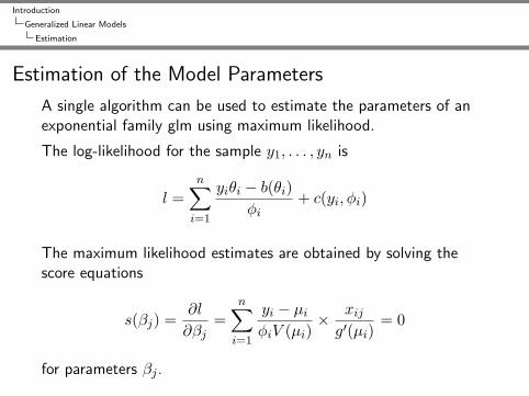
Estimation of the Model Parameters

A single algorithm can be used to estimate the parameters of anexponential family glm using maximum likelihood.

The log-likelihood for the sample y1, . . . , yn is

l =n∑i=1

yiθi − b(θi)φi

+ c(yi, φi)

The maximum likelihood estimates are obtained by solving thescore equations

s(βj) =∂l

∂βj=

n∑i=1

yi − µiφiV (µi)

× xijg′(µi)

= 0

for parameters βj .

Introduction


Estimation

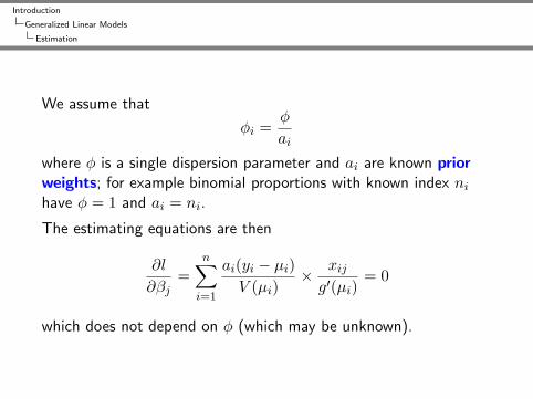
We assume that

φi =φ

ai

where φ is a single dispersion parameter and ai are known priorweights; for example binomial proportions with known index nihave φ = 1 and ai = ni.

The estimating equations are then

∂l

∂βj=

n∑i=1

ai(yi − µi)V (µi)

× xijg′(µi)

= 0

which does not depend on φ (which may be unknown).

Introduction


Estimation

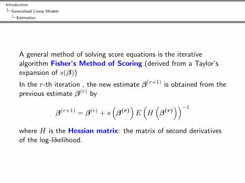
A general method of solving score equations is the iterativealgorithm Fisher’s Method of Scoring (derived from a Taylor’sexpansion of s(β))

In the r-th iteration , the new estimate β(r+1) is obtained from theprevious estimate β(r) by

β(r+1) = β(r) + s(β(r)

)E(H(β(r)

))−1

where H is the Hessian matrix: the matrix of second derivativesof the log-likelihood.

Introduction


Estimation

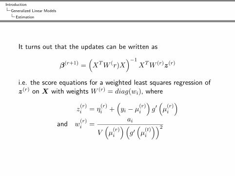
It turns out that the updates can be written as

β(r+1) =(XTW (r)X

)−1XTW (r)z(r)

i.e. the score equations for a weighted least squares regression ofz(r) on X with weights W (r) = diag(wi), where

z(r)i = η

(r)i +

(yi − µ(r)

i

)g′(µ

(r)i

)and w

(r)i =

ai

V(µ

(r)i

)(g′(µ

(t)i

))2

Introduction


Estimation

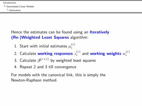
Hence the estimates can be found using an Iteratively(Re-)Weighted Least Squares algorithm:

1. Start with initial estimates µ(r)i

2. Calculate working responses z(r)i and working weights w

(r)i

3. Calculate β(r+1) by weighted least squares

4. Repeat 2 and 3 till convergence

For models with the canonical link, this is simply theNewton-Raphson method.

Introduction


Estimation

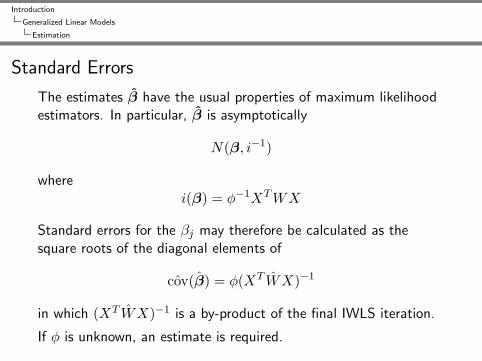
Standard Errors

The estimates β have the usual properties of maximum likelihoodestimators. In particular, β is asymptotically

N(β, i−1)

wherei(β) = φ−1XTWX

Standard errors for the βj may therefore be calculated as thesquare roots of the diagonal elements of

ˆcov(β) = φ(XT WX)−1

in which (XT WX)−1 is a by-product of the final IWLS iteration.

If φ is unknown, an estimate is required.

Introduction


Estimation

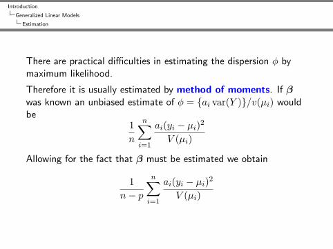
There are practical difficulties in estimating the dispersion φ bymaximum likelihood.

Therefore it is usually estimated by method of moments. If βwas known an unbiased estimate of φ = {ai var(Y )}/v(µi) wouldbe

1n

n∑i=1

ai(yi − µi)2

V (µi)

Allowing for the fact that β must be estimated we obtain

1n− p

n∑i=1

ai(yi − µi)2

V (µi)

Introduction

GLMs in R

glm Function

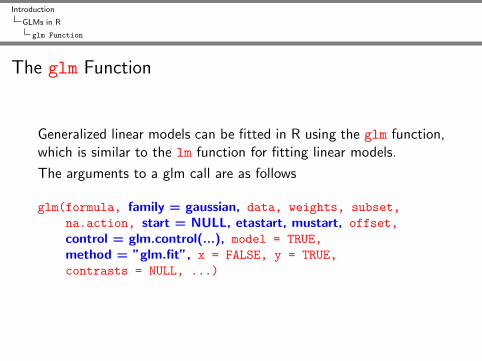
The glm Function

Generalized linear models can be fitted in R using the glm function,which is similar to the lm function for fitting linear models.

The arguments to a glm call are as follows

glm(formula, family = gaussian, data, weights, subset,na.action, start = NULL, etastart, mustart, offset,control = glm.control(...), model = TRUE,method = ”glm.fit”, x = FALSE, y = TRUE,contrasts = NULL, ...)

Introduction

GLMs in R

glm Function

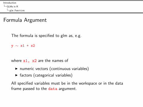
Formula Argument

The formula is specified to glm as, e.g.

y ∼ x1 + x2

where x1, x2 are the names of

I numeric vectors (continuous variables)

I factors (categorical variables)

All specified variables must be in the workspace or in the dataframe passed to the data argument.

Introduction

GLMs in R

glm Function

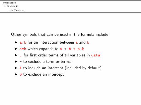
Other symbols that can be used in the formula include

I a:b for an interaction between a and b

I a*b which expands to a + b + a:b

I . for first order terms of all variables in data

I - to exclude a term or terms

I 1 to include an intercept (included by default)

I 0 to exclude an intercept

Introduction

GLMs in R

glm Function

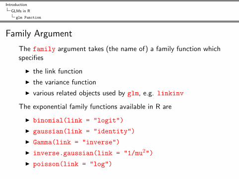
Family Argument

The family argument takes (the name of) a family function whichspecifies

I the link function

I the variance function

I various related objects used by glm, e.g. linkinv

The exponential family functions available in R are

I binomial(link = "logit")

I gaussian(link = "identity")

I Gamma(link = "inverse")

I inverse.gaussian(link = "1/mu2")

I poisson(link = "log")

Introduction

GLMs in R

glm Function

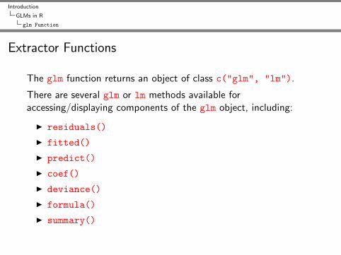
Extractor Functions

The glm function returns an object of class c("glm", "lm").

There are several glm or lm methods available foraccessing/displaying components of the glm object, including:

I residuals()

I fitted()

I predict()

I coef()

I deviance()

I formula()

I summary()

Introduction

GLMs in R

Example with Normal Data

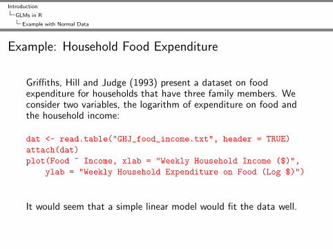
Example: Household Food Expenditure

Griffiths, Hill and Judge (1993) present a dataset on foodexpenditure for households that have three family members. Weconsider two variables, the logarithm of expenditure on food andthe household income:

dat <- read.table("GHJ_food_income.txt", header = TRUE)attach(dat)plot(Food ~ Income, xlab = "Weekly Household Income ($)",

ylab = "Weekly Household Expenditure on Food (Log $)")

It would seem that a simple linear model would fit the data well.

Introduction

GLMs in R


We will first fit the model using lm, then compare to the resultsusing glm.

foodLM <- lm(Food ∼ Income)summary(foodLM)foodGLM <- glm(Food ∼ Income)summary(foodGLM)

Introduction

GLMs in R


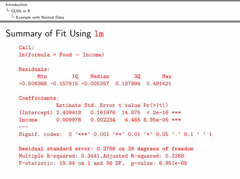
Summary of Fit Using lm

Call:

lm(formula = Food ∼ Income)

Residuals:

Min 1Q Median 3Q Max

-0.508368 -0.157815 -0.005357 0.187894 0.491421

Coefficients:

Estimate Std. Error t value Pr(>|t|)

(Intercept) 2.409418 0.161976 14.875 < 2e-16 ***

Income 0.009976 0.002234 4.465 6.95e-05 ***

---

Signif. codes: 0 ’***’ 0.001 ’**’ 0.01 ’*’ 0.05 ’.’ 0.1 ’ ’ 1

Residual standard error: 0.2766 on 38 degrees of freedom

Multiple R-squared: 0.3441,Adjusted R-squared: 0.3268

F-statistic: 19.94 on 1 and 38 DF, p-value: 6.951e-05

Introduction

GLMs in R


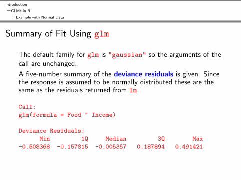
Summary of Fit Using glm

The default family for glm is "gaussian" so the arguments of thecall are unchanged.

A five-number summary of the deviance residuals is given. Sincethe response is assumed to be normally distributed these are thesame as the residuals returned from lm.

Call:glm(formula = Food ~ Income)

Deviance Residuals:Min 1Q Median 3Q Max

-0.508368 -0.157815 -0.005357 0.187894 0.491421

Introduction

GLMs in R


The estimated coefficients are unchanged

Coefficients:Estimate Std. Error t value Pr(>|t|)

(Intercept) 2.409418 0.161976 14.875 < 2e-16 ***Income 0.009976 0.002234 4.465 6.95e-05 ***---Signif. codes: 0 ’***’ 0.001 ’**’ 0.01 ’*’ 0.05 ’.’ 0.1 ’ ’ 1

(Dispersion parameter for gaussian family taken to be 0.07650739

Partial t-tests test the significance of each coefficient in thepresence of the others. The dispersion parameter for the gaussianfamily is equal to the residual variance.

Introduction

GLMs in R


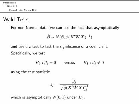
Wald Tests

For non-Normal data, we can use the fact that asymptotically

β ∼ N(β, φ(X ′WX)−1)

and use a z-test to test the significance of a coefficient.

Specifically, we test

H0 : βj = 0 versus H1 : βj 6= 0

using the test statistic

zj =βj√

φ(X ′WX)−1jj

which is asymptotically N(0, 1) under H0.

Introduction

GLMs in R


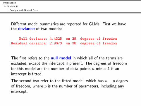
Different model summaries are reported for GLMs. First we havethe deviance of two models:

Null deviance: 4.4325 on 39 degrees of freedomResidual deviance: 2.9073 on 38 degrees of freedom

The first refers to the null model in which all of the terms areexcluded, except the intercept if present. The degrees of freedomfor this model are the number of data points n minus 1 if anintercept is fitted.

The second two refer to the fitted model, which has n− p degeesof freedom, where p is the number of parameters, including anyintercept.

Introduction

GLMs in R


Deviance

The deviance of a model is defined as

D = 2φ(lsat − lmod)

where lmod is the log-likelihood of the fitted model and lsat is thelog-likelihood of the saturated model.

In the saturated model, the number of parameters is equal to thenumber of observations, so y = y.

For linear regression with Normal data, the deviance is equal to theresidual sum of squares.

Introduction

GLMs in R


Akiake Information Criterion (AIC)

Finally we have:

AIC: 14.649

Number of Fisher Scoring iterations: 2

The AIC is a measure of fit that penalizes for the number ofparameters p

AIC = −2lmod + 2p

Smaller values indicate better fit and thus the AIC can be used tocompare models (not necessarily nested).

Introduction

GLMs in R


Residual Analysis

Several kinds of residuals can be defined for GLMs:

I response: yi − µiI working: from the working response in the IWLS algorithm

I Pearson

rPi =yi − µi√V (µi)

s.t.∑

i(rPi )2 equals the generalized Pearson statistic

I deviance rDi s.t.∑

i(rDi )2 equals the deviance

These definitions are all equivalent for Normal models.

Introduction

GLMs in R


Deviance residuals are the default used in R, since they reflect thesame criterion as used in the fitting.

For example we can plot the deviance residuals against the fittedvalues ( on the response scale) as follows:

plot(residuals(foodGLM) ~ fitted(foodGLM),xlab = expression(hat(y)[i]),ylab = expression(r[i]))

abline(0, 0, lty = 2)

Introduction

GLMs in R


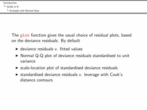
The plot function gives the usual choice of residual plots, basedon the deviance residuals. By default

I deviance residuals v. fitted values

I Normal Q-Q plot of deviance residuals standardised to unitvariance

I scale-location plot of standardised deviance residuals

I standardised deviance residuals v. leverage with Cook’sdistance contours

Introduction

GLMs in R


Residual Plots

For the food expenditure data the residuals do not indicate anyproblems with the modelling assumptions:

plot(foodGLM)

Introduction

Exercises

Exercises

1. Load the SLID data from the car package and attach the dataframe to the search path. Look up the description of the SLIDdata in the help file.

In the following exercises you will investigate models for the wagesvariable.

2. Produce appropriate plots to examine the bivariate relationshipsof wages with the other variables in the data set. Which variablesappear to be correlated with wages?

3. Use lm to regress wages on the linear effect of the othervariables. Look at a summary of the fit. Do the results appear toagree with your exploratory analysis? Use plot to check theresiduals from the fit. Which modelling assumptions appear to beinvalid?

Introduction

Exercises

4. Repeat the analysis of question 3 with log(wages) as theresponse variable. Confirm that the residuals are more consistentwith the modelling assumptions. Can any variables be droppedfrom the model?

Investigate whether two-way and three-way interactions should beadded to the model.

Introduction

Exercises

In the analysis of question 4, we have estimated a model of theform

log yi = β0 +p∑r=1

βrxir + εi (1)

which is equivalent to

yi = exp

(β∗0 +

p∑r=1

βrxir

)× ε∗i (2)

where εi = log(ε∗i )− E(log ε∗i ).

Introduction

Exercises

Assuming εi to be normally distributed in Equation 1 implies thatlog(Y ) is normally distributed. If X = log(Y ) ∼ N(µ, σ2), then Yhas a log-Normal distribution with parameters µ and σ2. It can beshown that

E(Y ) = exp(µ+

12σ2

)var(Y ) =

{exp(σ2)− 1

}{E(Y )}2

so thatvar(Y ) ∝ {E(Y )}2

An alternative approach is to assume that Y has a Gammadistribution, which is the exponential family with thismean-variance relationship. We can then model E(Y ) using aGLM. The canonical link for Gamma data is 1/µ, but Equation 2suggests we should use a log link here.

Introduction

Exercises

5. Use gnm to fit a Gamma model for wages with the samepredictor variables as your chosen model in question 4. Look at asummary of the fit and compare with the log-Normal model – Arethe inferences the same? Are the parameter estimates similar?Note that t statistics rather than z statistics are given for theparameters since the dispersion φ has had to be estimated.

6. (Extra time!) Go back and fit your chosen model in question 4using glm. How does the deviance compare to the equivalentGamma model? Note that the AIC values are not comparable here:constants in the likelihood functions are dropped when computingthe AIC, so these values are only comparable when fitting modelswith the same error distribution.

Introduction to Generalized Linear Models · Generalized linear models extend the general linear...

Documents

Transcript of Introduction to Generalized Linear Models · Generalized linear models extend the general linear...