Mount Campbell Choueiki Long-Run Marginal Cost
163
A METHOD TO ESTIMATE LONG-RUN MARGINAL COST OF SWITCHING FOR BASIC TELEPHONE SERVICE CUSTOMERS Clark A. Mount-Campbell Associate Professor Industrial & Systems Engineering Hisham M. Choueiki Graduate Research Associate THE NATIONAL REGULATORY RESEARCH INSTITUTE 1080 Carmack Road Columbus, Ohio 43210 September 1987 NRRI 87-17 This report was prepared by The National Regulatory Research Institute under contract to the Public Utilities Commission of Ohio (PUCO). The views and opinions of the authors do not necessarily state or reflect the views, opinions, or policies of PUCO or The National Regulatory Research Institute. Reference to trade names or specific commercial products, commodities or services in this report does not represent or constitute an endorsement, recommendation, or favoring by PUCO or The National Regulatory Research Institute of the specific commercial product, commodity or service.
Transcript of Mount Campbell Choueiki Long-Run Marginal Cost
A METHOD TO ESTIMATE LONG-RUN MARGINAL COST OF SWITCHING FOR BASIC TELEPHONE SERVICE CUSTOMERS
Clark A. Mount-Campbell Associate Professor Industrial & Systems Engineering
Hisham M. Choueiki Graduate Research Associate
THE NATIONAL REGULATORY RESEARCH INSTITUTE 1080 Carmack Road
Columbus, Ohio 43210
September 1987
NRRI 87-17
This report was prepared by The National Regulatory Research Institute under contract to the Public Utilities Commission of Ohio (PUCO). The views and opinions of the authors do not necessarily state or reflect the views, opinions, or policies of PUCO or The National Regulatory Research Institute.
Reference to trade names or specific commercial products, commodities or services in this report does not represent or constitute an endorsement, recommendation, or favoring by PUCO or The National Regulatory Research Institute of the specific commercial product, commodity or service.

EXECUTIVE SUMMARY
In this study we develop and examine a method to estimate a cost of "plain old telephone service" (POTS) that would be helpful in setting prices. POTS is defined to consist of an access line to a local network switch that will connect, on demand, the access line with other local access lines. In addition, POTS should provide the capability of connecting with a nationwide network switch, but the act of making that connection and the telephone call that would ensue is not part of POTS.
The main issues in the study are: What are the appropriate costs? Can the appropriate cost for POTS be separated from the costs for other services? What methods can be used to compute a cost figure for each part of the local network and aggregate them for the entire company? How can the cost figures be annualized?
Long-run marginal cost l is a most useful and appropriate item of information for setting prices. It is an important input for a number of pricing methods although not the only input. Demand information is also an important input to the pricing decision. The problem was also viewed from a decision theoretic point of view. In this alternative approach we examine the level of revenues that would provide adequate economic motivation to cause a telephone company to decide to add capacity. Such a method can derive a cost by applying engineering economic principles routinely used in the telephone industry for making capacity and configuration decisions.
The decision theoretic approach yields a cost that, in theory, is the same as a long-run marginal cost. In reality, because the equipment is available only in "lumps" which are added to existing facilities the decision theoretic approach results in an estimate of a constrained, average incremental cost and is considered here to be the superior method.
A telephone system consists of three distinct components: switching facilities, interswitch network facilities, and subscriber loop. The costs of expanding each of these facilities was assumed to be separably determinable with a total cost obtained by adding the individual component costs. While no empirical data exists to support or refute this assumption, the separability of the engineering function, and the separability of the activities for expanding these facilities suggest that the assumption is reasonable. However, the method of determining expansion costs must be
1 Long-run marginal costs may be thought of as the current (not historical) cost of serving one additional customer where all resources are optimally varied to provide that service. If only a few inputs are varied then it is a short-run marginal cost.
iii
uniquely developed for each facility type. In this report we developed a method for switching facilities and tested it in a pilot test with one actual switching machine.
A first goal of the method is to model the incremental costs. The model is then used to simulate those costs that a firm would compare with incremental revenues in order to economically justify the addition of new plant. The per-unit average incremental cost developed by the method will mathematically approximate a constrained long-run marginal cost. The constraint is that the modelled'costs represent those for expanding existing facilities rather than those for constructing new facilities. Finally, an annual equivalent of the incremental cost is recommended so as to take tax effects and fill-rate forecasts into account and to move the one-time incremental cost closer to a rental price. The steps of the method are:
1. Select a sample of switches.
2. Establish an ESS lA equivalent switch design for the non-ESS switches in the sample.
3. Have the company design expansions for the sample switches according to an experimental plan.
4. Organize the equipment lists for the expansion plans and examine for inconsistent patterns -- request revised designs when needed.
5. Fit a spline function regression model to four different sized expansions.
6. Compute an average annual unit cost for each output variable.
7. Compute an average annual cost per customer for residential and business customers.
The key step in the method is step 3. Rather than examine actual switch expansions where capacity to perform both POTS and non-POTS functions have been added, step 3 asks the telephone company engineers to use their computer aided design methods to design switch expansions according to an experimental plan that will allow separate estimation of the costs of the POTS functions. This approach unconfounds the costs of POTS and non-POTS functions that are generally confounded in data from actual expansions. The approach may be likened to performing controlled laboratory experiments. When an expansion is planned, it is described in terms of the following variables:
.. access lines 01> intraswitch busy-hour usage & interswitch busy-hour usage 01> DID trunks
The models in step 5 give expansion costs as a function of these variables. In the pilot study, interexchange busy-hour usage was also a variable. Its cost was found to be linearly separable from the other costs making it possible to hold it fixed in subsequent experiments. In some
iv

cases, DID trunk cost was not linearly separable from the other costs and was therefore retained as an experimental variable. The addition of a POTS customer is thought to affect only the first three variables listed above. Thus, given usage patterns for a POTS customer, it is known how the first three variables are affected by the addition to the system of POTS customers. Then from the cost models one can determine the construction costs of the added capacity.
Step 6 converts the construction costs to annual equivalent costs; taking into account income taxes, capital structure, depreciation rates, allowed rate of return, the rate at which customers are forecasted to fill the capacity, and (when available) operation and maintenance costs. The result is an annual cost for each of the variables listed above for each switch in the sample of switches selected in step 1. These costs per switch are then averaged across sample switches ~~ such a way as ~n account for differential rates of growth in POTS customers at these offices.
Finally, step 7 computes the long-run marginal (or its practical equivalent--average incremental) cost for POTS customer based on their usage pattern.
A pilot study of the method was performed on a single Ohio Bell office. This pilot consisted of steps 2 through 5 and a part of 6 on that one office rather that a sample of several offices as prescribed in step 1. Steps 6 and 7 were demonstrated by simulating them using the results from the actual pilot office augmented with hypothetical (but plausable) data for two other offices to complete a sample of size 3. The result of app-lying steps 1 through 5 and part of 6 to the pilot switch was obtained under the following assumptions: capital structure is 40% debt with an average return of 9% on debt and a composit cost of capital of 13.2%; income tax rate was 46%; regulatory book life was 10 years and tax life was 5 years using an ACRS depreciation schedule. With these assumed values and actual cost values for the proposed expansion the optimal plan called for building three years worth of additional capacity at the beginning of year 1. This resulted in an annual cost of $3.24 per access line, $1.10 per intraswitch busy-hour CCS (centrum call seconds) and $22.18 per interswitch busy-hour CCS. These costs do not include operation and maintenance costs for the new facility nor do they include a fixed cost of $135,000 per switch expansion. This latter figure annualizes (under the above assumptions) to $23.13 per line. For a hypothetical POTS customer requiring 1 access line, 0.6 CCS of busyhour intraswitch usage, and 1.3 CCS of busy-hour interswitch usage, the annual cost of that customer to the system would be $32.73, excluding the $23.13 fixe'd cost per line. If the fixed cost is allocated on the basis of lines, the total cost would be $55.86 of annual switching cost per customer .7
While the method developed in this study does involve some expense for the telephone company in responding to step 3, it does not appear to be an excessive cost nor does it require an activity that is not ordinarily engaged in by telephone company engineers. It does provide data that are absent of confounding and allows the determination of costs for POTS separately from other services. Furthermore, it provides a cost figure representing the annual revenues needed for economic motivation to decide to
v
expand facilities, and provides practical means to treat the problems of "lumpyll investment, forecasted growth rates, and expansions that are constrained by existing facilities.
vi
TABLE OF CONTENTS
LIST OF FIGURES . . LIST OF TABLES. FOREWORD. . . . ACKNOWLEDGEMENTS.
Chapter
1
2
3
4
Appendix
A
B
C
D
INTRODUCTION ..
Definition of Plain Old Telephone Service .. The Problem ......... -Organization of the Report
APPROPRIATE COSTS . .
Introduction Production Functions and Marginal Costs ... Summary and Conclusion . . . . . . . '.'
A METHOD FOR ESTIMATING THE MARGINAL CAPITAL COST IN A CENTRAL OFFICE SWITCH .
Introduction . . . . . . . Total Marginal Cost. . . . . Cost Study Method for COE. . Method Rationale . . . . . Detail Analysis of Steps . . Summary and Findings . . . .
CONCLUSIONS AND RECOMMENDATIONS .
TECHNICAL DISCUSSION ... 4-1
2 FRACTIONAL FACTORIAL EXPERIMENTAL CONSTRUCTION PLAN ...... '.' .. .
3-1 2 FRACTIONAL FACTORIAL EXPERIMENTAL CONSTRUCTION PLAN . . . . . . .
THE CAPCOST PROGRAM DESCRIPTION .
vii
viii ix xi
xiii
1
1 3 3
5
5 8
13
15
15 15 18 21 25 60
63
65
107
125
135
Figure
3-1
3-2
3-3
LIST OF FIGURES
Analysis of Cost . . .
Contribution of Access Lines to Expansion Costs.
Contribution of Intraoffice Traffic to Expansion Costs . . . . . . . . . .
3-4 Contribution of Interoffice Traffic to
3-5
3-6
3-7
3-8
3-9
Expansion Costs . . . . . . . . . .
Average Interoffice Traffic Contribution to Expansion Costs . . . . . . .
Contribution of Access Lines to Total Expansion Costs . . . . . . .
Contribution of Intraoffice Traffic to Expansion Costs . . . . . . . . . .
Contribution of Interoffice Traffic to Total Expansion Costs . . . . . . . .
Average Interoffice Traffic Contribution to Total Expansion Costs . . . . . . . .
viii
17
28
29
29
30
30
31
31
32
LIST OF TABLES
Page
3-1 Equipment Required for Size 1 Expansion 37
3-2 Equipment Required for Size 2 Expansion 38
3-3 Equipment Required for Size 3 Expansion 39
3-4 Equipment Required for Size 4 Expansion 40
3-5 Differential Equipment Required for Size 2 Expansion . . . . .. ............ 41
3-6 Differential Equipment Required for Size 3 Expansion . . . . .. ............ 42
3-7 Differential Equipment Required for Size 4 Expansion . . . . .. ............ 43
3-8 Example of Flawed Differential Size 3 Expansion 44
3-9 Data Set for Size 1 Expansion 46
3-10 Data Set for Size 2 Expansion 46
3-11 Data Set for Size 3 Expansion 47
3-12 Data Set for Size 4 Expansion 47
3-13 The Coefficients of the Capital Cost (y ) c Model of Switch Expansions .............. 49
3-14 The Coefficients of the Total Cost (Yt) Model of Switch Expansions . . . . . . . . . . 50
3-15 Three Cases for the Value of X4 While Computing x 2 's Cost .. 51
3-16 Forecasted Growth By Office: Hypothetical Data. . . 53
3-17 Capital Cost Model ..... 55
3-18 The Average Annual Per Unit Cost for Three Variables in Three Switches ............... 58
ix

FOREWORD
This report was done under contract to the Public Utilities Commission
of Ohio. PUCO has generously allowed us to publish it for general
distribution. Its subject--determining the marginal cost of Plain Old
Telephone Service--is timely and of wide interest.
xi
Douglas N. Jones Director, NRRI Columbus, Ohio
December 30, 1987

1
1
1
1
1
1
1
1
1
1
1
1
1
1
1
1
1
1
1
. 1
1
1
1
1
1
1
1
1
1
1
1
1
1
1
1
1
1
1
1
ACKNOWLEDGEMENTS
The authors would like to express their appreciation to the Ohio Bell
Telephone Company and especially the engineers and regulatory affairs staff
members who gracefully accepted the onerous task of responding to our data
requests.
In addition, we thank the Public Utilities Commission of Ohio for
funding the project. It was invaluable having the personal interest and
support of John Borrows and Diane Hockman for this project. It was through
their efforts that information could pass from Ohio Bell to us, A debt is
owed to Roger Montgomery who offered many helpful suggestions.
We are especially grateful to Carole Prutsman and Wendy Windle, who. in
the eleventh hour, cheerfully bore the task of converting and correcting our
word processor files to the NRRI system.
xiii

CHAPTER I
INTRODUCTION
Definition of POTS <Plain Old Telephone Service)
The break-up of AT&T, the Computer I and II inquiries, and the Access
Charge ruling are among the recent significant events in the evolution of
national communications policy. These macro policy changes have been an
enormous force for change in the way state governments can and should
regulate the telephone companies in their jurisdictions. Additionally,
technological advances in fiber optics, digital communications, and
satellite communications have resulted in reduced costs for these
technologies, making them competitive with, and in many cases superior to
the older communications technologies that dominate the existing
communications infrastructure in this country. These newer technologies
also increase the variety of ancillary communication services that can be
offered at reasonable prices. The main thrust of this evolving national
policy has been to encourage competition in those markets where competition
appears feasible because of technological advances.
One market that thus far seems to have been relatively unaffected by
the changes in policy and technology is the market for "plain old telephone
service" (POTS). POTS is normally thought to consist of an access line to a
local network switch that will connect, on demand,. the access line with
other local access lines. Generally, the public would also expect POTS to
provide the capability of connecting with a nationwide network switch, but
the act of connecting to the nationwide network and the telephone call that
would ensue is not part of POTS; instead, it is a part of the interexchange
communication market that national policy intends to make competitive. This
capability of connecting to a nationwide network is the part of POTS that
causes us to refer to POTS as being " re l a tively" unchanged by policy and
technology. The fact is, this part of POTS has been opened up to
competition for large users of interexchange services. This competition is
characterized by a user electing to connect to an interexchange carrier
I
without using the POTS capability. When this happens the term "bypass" is
applied.
It has been argued that the main reason bypass is economically feasible
and, therefore, competitive with POTS, is that there is incorrect pricing of
the interexchange calls made through POTS lines. Others argue that, even if
interexchange calls made through POTS lines were priced correctly, some
IIbypass ll would still occur. The reason is that a user may need to increase
his capacity to make and receive interexchange calls, but does not need to
increase his capacity to make or receive local calls. If the user's
interexchange capacity is increased by adding POTS lines, then he would get
and pay for an increase in capacity for both local and interexchange
calling. In fact, some users may already have more POTS lines than needed
for their local calls simply because they are needed for interexchange
calls. Such users could also benefit from bypassing the local network.
All this brings into question whether it makes sense to include as a
part of POTS the capability of connecting to a nationwide switch network.
Our conclusion is that POTS should include this capability, primarily
because as long as interexchange carriers have access to an exchange there
is no cost to the POTS subscribers associated with having the capability of
accessing them, but given the presently used telecommunications technology,
there would be additional cost incurred if the telephone company had to
provide a "local call only" type of POTS service. Of course, in the
unlikely event that no interexchange carrier desired access to a particular
exchange, then presumably the local telephone company would be obligated to
invest in interexchange equipment in order to provide the "capability" to
its POTS users. Such costs would be passed to the POTS users only if the
use of the interexchange facility was not sufficient to cover its cost.
Since this latter case would be a most unusual situation we prefer to
discard it as a possibility. Thus, for purposes of this study, POTS, which
is also the focus of the study, is defined to include the capability of
connecting to a nationwide network, and that any competition that capability
may have from lIinterexchange service only" types of bypass services is an
irrelevant factor.
2
The Problem
The problem is that there are many services offered by a telephone
company besides POTS. Many of these services are subject to competition
whether or not they are actively regulated. It is also the case that the
design of present-day central office equipment integrates into one machine
many functions that are used in a variety of ways to offer both competitive
services and POTS. If a commission is to move towards cost-based rates for
POTS, the question is how can one determine the appropriate costs? The
purpose of this study is to explore that question, to develop an approach
for computing appropriate costs, and to assess the feasibility of the
approach.
The main issues in this study are: What are the appropriate costs?
Can the appropriate cost for 'POTS be separated from the costs for other
services? What methods can be used to compute a cost figure for each part
of the local network and aggregate them for the entire company? How can the
cost figures be annualized? What are the pros and cons of the methods?
While some of these issues are pursued, the main empirical work is focused
on central office equipment (COE) of the electronic switching system (ESS)
type. This represents a common and current technology, although telephone
companies are beginning to move toward digital technology. As we examine
the details of the issues we will find a number of additional subissues such
as "lumpiness of investment," and how or whether to consider forecasts.
Organization of the Report
In chapter 2 there is a theoretical discussion of what costs might be
appropriate and useful in setting rates for POTS services approached from
two points of view. One is based on rudimentary economic theory, while the
other is a decision theoretic viewpoint. Sufficient conditions for the
equivalence of these two views of the problem are given. Chapter 3 presents
a method for acquiring data and computing the types of costs defined in
chapter 2. To illustrate the method, actual results from the empirical
study of one Ohio Bell office are used. While this empirical work has been
a major part of the study, the purpose is to derive a method to determine
long-run marginal costs and it is in the context of the method itself that
3

the empirical results are presented. In addition, there is a technical
appendix that gives the empirical results. Chapter 4 contains conclusions
and recommendations.
Appendix A contains a description of the analysis method used on data
obtained in the pilot study of one Ohio Bell office. The data request for
acquiring the Ohio Bell data is also found in appendix A. Appendix B is
comprised of a data request form similar to the one used in the pilot study,
but reduced to reflect a more efficient experimental plan than the one used
in the pilot study. Appendix C presents the same sort of data request as
appendix B but the experimental plan has been 'further reduced to an ultra
efficient form with respect to the amount of data it requests. Finally, as
part of the project a Lotus spreadsheet program was developed to convert
investment costs into annual equivalent costs. These annual equivalent
costs include the effect of income taxes, probabilistic lives, equipment
fill rates, and operation and maintenance expenses. Appendix D is a
description of the program and instructions on its use.
4
CHAPTER 2
APPROPRIATE COSTS
Introduction
According to economic theory, a profit maximizing firm that sells its
product in competitive markets will determine its production level such that
the long-run marginal cost of one more unit of product is equal to its
market price. If the same firm enjoys a monopoly in the market place then
it will sell its product at its long-run marginal cost plus an adjustment
that is based on the rate of change of the price with respect to a change in
the quantity produced. In another approach, Baumol and Bradford have
suggested the use of Ramsey prices for monopoly enterprises. 1 The Ramsey
prices are selected to maximize the welfare of both producers and consumers.
Like the monopoly prices, they are equal to adjusted long-run marginal
costs. In this case, the adjustment is proportional to the inverse of the
price elasticity for the product. The cornmon factor in all these approaches
is clearly long-run marginal cost. This does not mean that long-run
marginal cost is the best cost figure on which to base prices, but is a
useful cost to compute.
In the decision theoretic approach, we ask the question "what revenues
would be sufficient to motivate the firm to add the capacity to produce
additional units of a product?" Ignoring for the moment the uncertainty
inherent in such a decision making situation, the answer to the question can
be found in the engineering economy literature which is mainly concerned
with the analysis of decision problems of this type. 2 One notes that the
network and facilities planning activities in a telephone company are mainly
1 Baumol, W.J., and D.F. Bradford, "Optimal Departures from Marginal Cost Pricing," American Economic Review 60 (June 1970), pp. 265-283. 2 See, for example, Grant, E.L., W.G. Ireson, and K.S. Leavenworth, Principles of Engineering Economy, Seventh Edition, John Wiley & Sons, Inc., New York, 1982.
5
concerned with the analysis of decision problems of this type. If the
present worth of the incremental revenues derived from the additional
product is equal to or greater than the present worth of the minimum
incremental cost of producing the additional product, the decision would be
to add the capacity and increase production. In these problems the "cost of
capital" is normally the interest rate used to discount the prospective cash
flows to their present worth. Several different definitions for cost of
capital can apply, but a composite cost of capital based on the weighted
average cost of capital from all sources is the usual definition for a
large, widely-held corporation. Instead of present worth, an annualizing
calculation is sometimes used, and the comparison then is between the annual
equivalent revenue increase and the annual equivalent cost.
Regardless which calculation is used to make the decision, if the
increment of added capacity is one unit of product, then (under certain
conditions which are discussed later) the decision criteria given above is
really based on a long-run marginal cost. Since the calculations used in
the decision theoretic approach include discounting the incremental cash
flows at the cost of capital, it is easy to show that if the incremental
product is priced below its long-run marginal cost, the present worth of the
incremental revenues would be less than the present worth of the incremental
costs, and the company would decide not to add the capacity. If the firm)
did decide to disregard its decision criteria and add the capacity anyway,
the rate of return earned on the incremental investment would be less than
the cost of the capital needed to finance the capacity expansion.
Such an exercise is incomplete, of course, in the case of a regulated
utility. The regulated utility has an obligation to serve, and there are
service standards that include maximum time intervals that subscribers
should be made to wait before service is provided. Thus, if the service is
priced below marginal cost and there is enough demand that additional
capacity is needed, then to satisfy service standards the company is forced
to either: (1) add the capacity and earn less than the cost of capital, or
(2) find a short term way of satisfying the demand. In POTS service the
short-term way to satisfy demand would be to connect the subscribers to the
existing plant. This would cause its performance, as measured by blocked
calls (or lost calls), to deteriorate. Eventually, the repeated application
of the short-term solution would cause a decline in the quality of service.
6
Finally, enforcement of quality of service standards by a public service
commission would force the company to add the needed capacity at a rate of
return that is lower than the cost of capital.
If the cost of capital is the rate allowed by the regulatory commission
and if the commission sets a price below the long-run marginal cost, then,
in effect the commission will have contradicted itself. The contradiction
comes from allowing a certain rate of return and then, through service
standards, forcing the company to add capacity on which it will earn less
than the prescribed rate of return.
Thus, the decision theoretic approach ha~ appeal because it leads to a
pricing principle without making assumptions about markets or about the
profit maximizing objectives of the firm. That principle is that if a price
stimulates enough demand to require additional capacity, the revenues
generated from the demand at that price should be just sufficient to cause
the company (while using standard engineering economy decision analysis
techniques) to decide to add the capacity. Another way to express it is
that the price makes it economically attractive for the company to meet
service standards, thereby making it unnecessary to separately enforce the
service standards in a long-run situation. Short-run enforcement of service
standards is still needed to ensure that the timing of the company's long
run decision making does not unnecessarily inconvenience the subscriber,
that is, to ensure that the company takes the short-run steps necessary to
provide service until such time as the additional capacity becomes
available.
Although the principle stated above can be supplied with assumptions
that allow tracing the associated decision making back to a profit
maximizing firm, the absence of such assumptions does not prevent us from
being able to predict the economic behavior of the firm, whether or not it
is able to maximize profits. In fact, prices would have to be very
carefully set in order for the firm to maximize profits while following the
principle. Even when prices are different from those that maximize profit,
a firm is still better off following the principle.
Our conclusion is that long-run marginal cost is indeed a useful figure
to compute, and in view of the decision theoretic approach and the typical
service standards employed, the application of the above principle suggests
7
that long-run marginal cost is also an appropriate quantity to compute for
rate-making purposes.
Production Functions and Marginal Costs
In this section we summarize the relevant parts of the basic economic
theory of the firm presented by Intrilligator,3 and we relate this theory
to the decision theoretic ideas mentioned earlier. Also discussed are the
particular problems inherent in applying this theory to a real world
situation.
A key to the economic theory of the firm is the production function
which, in the single product firm, is the relationship between the maximum
quantity that can be produced in a given period of time and the quantities
of the factors of production that are inputs to the production process. The
exact nature of the function is dependent on the technology employed by the
industry in its production process. In its simplest form there are usually
two factors of production considered--labor and capital. In its more
complicated form the two factors can be disaggregated into many separate
factors. Examples are dividing labor into unskilled labor, skilled labor,
managerial labor, and dividing capital into land, production equipment, and
transport equipment. For our purposes here we shall consider the simpler
form of the function. Symbolically, the production function may be
represented as follows:
q = f(x, y)
where q is the quantity produced, f is the production function, x is the
amount of labor, and y the amount of capital input to the process. In the
event the firm is a multi"product firm, the production function is a vector
valued function rather than a scalar-valued function, and q then becomes a
vector. It is usually assumed that the production function is
differentiable and that the derivative is continuous.
To develop the theory, it is supposed that a firm will adjust its
output to some optimal level in the short-run by varying only one of the
3 Intrilligator, Michael D., Mathematical Optimization and Economic Theory, Prentice-Hall, Englewood Cliffs, N.J. (1971), pp. 178-219.
8
inputs (usually labor, since it is easiest to vary in the short run). As we
shall see, this idea will correspond to short-run marginal cost. In the
long-run a firm is able to optimally adjust all its inputs in order to
achieve an optimal production level. This situation will be seen to pertain
to a long-run marginal cost.
Beginning the definitions of marginal costs, we assume that the firm
does not have sufficient power in the supply side markets to affect the wage
rates for labor or the "rental" rates for capital. Let p and p represent, x y
respectively, the cost of one unit of labor for one period and the cost of
one unit of capital for one period, and suppose that q is a given level of
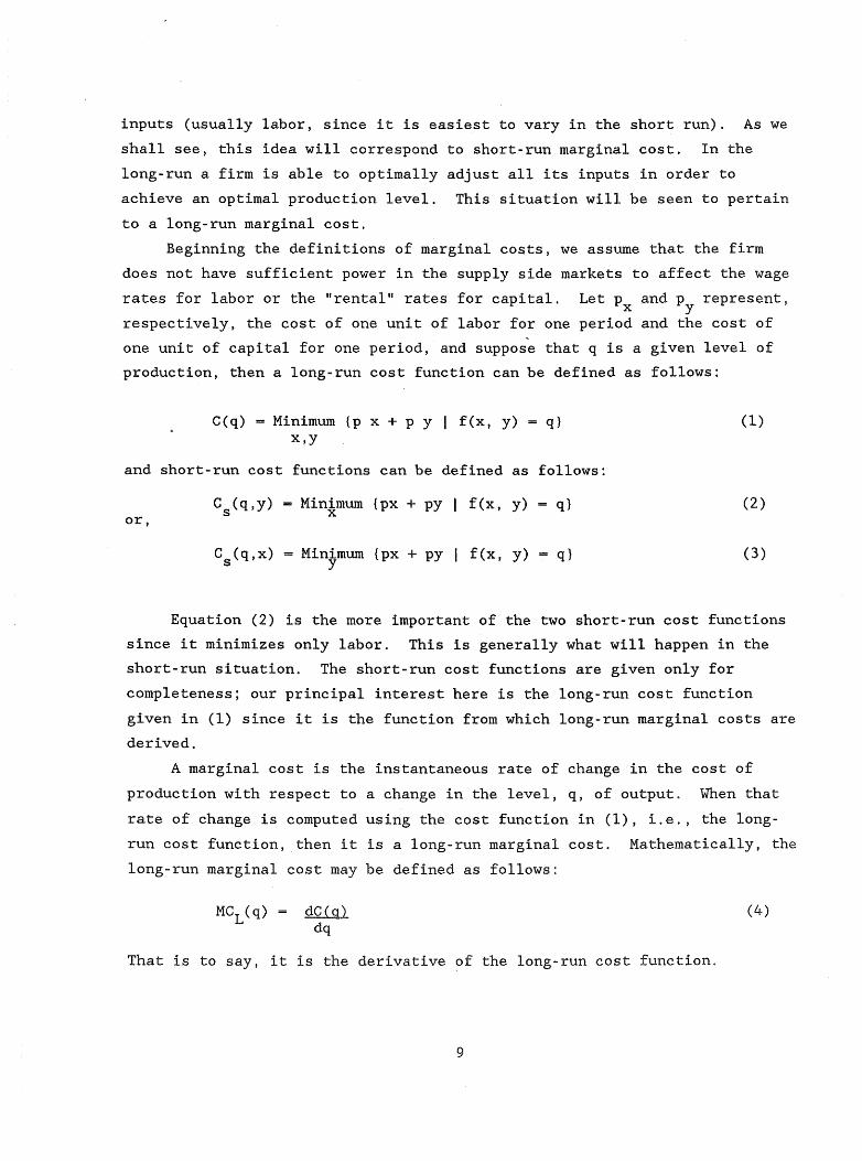
production, then a long-run cost function can be defined as follows:
C(q) Minimum {p x + p y I f(x, y) x,y
q}
and short-run cost functions can be defined as follows:
or, Minimum (px + py I f(x, y) = q} x
Minimum (px + py I f(x, y) y q}
(1)
(2)
(3)
Equation (2) is the more important of the two short-run cost functions
since it minimizes only labor. This is generally what will happen in the
short-run situation. The short-run cost functions are given only for
completeness; our principal interest here is the long-run cost function
given in (1) since it is the function from which long-run marginal costs are
derived.
A marginal cost is the instantaneous rate of change in the cost of
production with respect to a change in the level, q, of output. When that
rate of change is computed using the cost function in (1), i.e., the long
run cost function, then it is a long-run marginal cost. Mathematically, the
long-run marginal cost may be defined as follows:
flQ.Lgl dq
That is to say, it is the derivative of the long-run cost function.
9
(4)

Thus far, all the cost functions have depended on q which is as yet
undetermined, but Intrilligator shows that if the product of the firm is
sold in a competitive market at price p, then the firm will produce a
quantity q that makes the marginal cost equal to p. This is shown by
selecting a q that will optimize the following expression of profit:
Maximize pq - C(q) q
(5)
To examine how this theory relates to the decision theoretic approach
we first observe that if the q is a large enough value, then C(q+l) - C(q)
is a close mathematical approximation to the derivative of the long-run cost
function (i.e. t it approximates the long-run marginal cost),4 Second, we
observe that C(q+l) - C(q) is the incremental cost of one more unit of
production and p is the incremental revenue derived from that additional
unit of production. According to the decision theoretic approach, if p is
greater than or equal to C(q+l) - C(q), then the production should be
expanded the one additional unit; and as long as the incremental revenue is
greater or equal to the incremental cost, the capacity should be expanded
until a point is reached that the incremental cost exceeds the incremental
revenue. When this happens the last extra unit of production would not be
added. Thus, we see that the decision theoretic approach yields the same
solution as the classical economic theory.
In the case of a monopoly firm, the assumption is that the market price
of the product is influenced by the quantity that the firm decides to
produce, In such a situation the profit maximizing firm will choose a
quantity q to produce such that the long-run marginal costs are equal to the
marginal revenues. s Here again, the decision theoretic approach works to
maximize profits if the incremental revenues are estimated to be something
other than just p. In this case, the firm would consider the change in
revenues resulting from a price change that would be necessary to stimulate
demand for the incremental unit of production along with the revenues
generated by the incremental unit. The total revenue change would be the
4
S Other approximations could be C(q) - C(q-l) or [C(q+l) - C(q-I)]/2. Marginal revenue is the derivative of the price-quantity function.
10
incremental revenues that would then be compared with the incremental cost
in order to make the production capacity decision. The decision rule to
expand or not to expand is exactly the same as before.
We conclude that while the basic economic theory defines the problem of
the firm and specifies necessary conditions for maximizing profit, the
decision theoretic approach developed in the engineering economy literature
clearly applies the same concept in a mathematically approximate and
realistic manner. We also note that in the decision theoretic view, C(q+l)
-C(qi provides a useful and adequate definition of marginal cost, even
though it is really an incremental cost. There remain a number of
difficulties that must be resolved.
Not minor among the difficulties is the fact that in reality one does
not measure C(q+l) - C(q) in order to decide whether or not to add capacity.
The actual cost functions are highly constrained by the already existing
plant so that what is measured is the cost of supplementing the existing
plant, rather than the difference in cost of building two differently sized
facilities. This difficulty is due more to the inadequacy of the economic
theory discussed above (we deliberately chose a simple version of the
theory) than it is a measurement problem. In these more complex and more
realistic capacity determination problems, we find that the basic question
is: "Does one build the extra capacity now, does one build it later, or does
one not build it at all?" Here again, decision theoretic approaches are
well suited to making such decisions and would optimally trade-off the cost
of idle capacity built now with the present worth of incurring some extra
fixed construction costs later caused by adding to an existing facility.
In considering the timing of the expansion decision, the difficulty is
that the incremental costs and revenues that the decision would be based on
are dependent upon a forecast of the need for service. The Long-Run
Incremental Cost (LRIC) method developed by AT&T ran into difficulties at
the Federal Communication Commission (FCC) for a number of reasons, and one
of them was that it depended on forecasts. The view was that forecasts can
be manipulated to show virtually any cost desired, thus the FCC rejected the
11

LRIC in favor of a fully distributed cost method. 6 While we have been
unable to avoid the use of demand forecasts in the method presented in this
paper, our rule was to keep costs and forecasts separated as much as
possible. This allows us to clearly identify when and how the forecast has
an effect on the costs.
Still another difficulty occurs when we recognize that most investment
in telephone office equipment is "lumpy." By this we mean that the
productio!l function does not vary continuously, as is generally assumed in
economic theory. Indeed, expensive items like central processing units, or
line link networks each cause large jumps in dapacity when they are added to
a system. Thus, the production function that economic literature assumes to
have continuous derivatives has instead discontinuous derivatives, and at
perhaps a large number of points it has no derivative at all. Furthermore,
many whole sections of the curve that represents the cost function will have
a derivative of zero. These problems do not mean that the theory does not
apply. They do mean, as is the case with all theory, that it serves as a
guide and cannot be expected to lead directly to methods to estimate some
real quantity.
A continuous derivative is not a needed assumption when using the
decision theoretic approach, but again forecasting may playa role when we ~
compute an incremental cost. Instead of letting the increment equal to only
one unit of output as was suggested earlier, some of the lumpiness can be
smoothed out by consiaering larger increments and then computing a per unit
average incremental cost as an approximation. The problem is knowing how
many units to average over. When considering revenues the problem is
knowing at what rate revenues are produced. For example, in the first year
it may be that only 50% of the added capacity is utilized, while the second
and third years the figure may be 75% and 100%. This "fill rate," as we
shall call it, is dependent on the forecasts of demand, while the revenue
depends on the fill rate and incremental revenues per customer. Any
decision to expand facilities must take the fill rate into account in order
6 Revision to Tariff FCC No. 260 Private Line Service, Series 5000 CTELPAK), Memorandum Opinion and Order, 61 F.C.C. 2d 587 (1976).
12

to know whether the new facility will achieve revenue levels that would make
adding the equipment the economically correct decision.
It should be pointed out that the economic theory and the decision
theoretic approach discussed earlier have focused on the single product
firm. The fact is, telephone companies are multi-product firms although
this study is concerned with only one service--POTS. POTS itself may be
viewed as at least three products according to our earlier discussion of the
service. These are local access, toll access, and local busy-hour usage.
In this study we have further separated local busy-hour usage into
intraoffice local busy-hour usage and interoffice local busy-hour usage,
since the capacities for these two parts of the usage service are mainly
provided by different parts of the lA switch. In any case, if we find that
the structure of incremental costs is largely additive, then the separation
of the incremental costs into pieces for each IIsubproduct" is possible. The
major empirical work in this study was intended to identify and model the
structure of the incremental central office equipment costs in order to
determine if separation of costs is possible. That work is presented in the
next chapter.
Summary and Conclusion
In this chapter we have discussed the usefulness of long-run marginal
cost as an input to the pricing decision. The basic economic theory that
was reviewed provided a clear definition of long-run marginal costs as well
as a rationale for its role in establishing the behavior of the firm, given
either competitive or monopoly markets for the firm~s product. While the
theory is presented in terms of a firm determining production levels, the
relationship developed in the theory between price and long-run marginal
cost offers clear guidance on setting prices. The presentation of the
decision theoretic approach and its discussion seemed to more clearly
connect prices with costs in that it demonstrated which relationship between
the two would elicit the desired behavior of the firm with respect to
whether or not it provides additional service to additional customers. It
was also shown that under certain conditions (i.e., if incremental costs and
incremental revenues are measured correctly in the decision theoretic
approach), the decision theoretic approach is fully compatible with the
13
economic theory. The decision theoretic approach may also overcome some of
the potential difficulties that are present in the real world--difficulties
that usually foil the direct application of certain basic economic theory.
Our fundamental conclusion is that the decision theoretic approach
offers the greatest potential to be a practical tool for developing cost
based prices of POTS. The goal of the approach is to model the incremental
costs. The model is then used to simulate those costs that a firm would
compare with incremental revenues in order to economically justify the
addition of new plant. The per-unit average incremental cost developed by
the method will mathematically approximate a constrained long-run marginal
cost. The constraint is that the modeled costs represent those for
expanding existing facilities, rather than those for constructing new
facilities. Finally, an annual equivalent of the incremental cost is
recommended so as to take tax effects and fill-rate forecasts into account,
and to move the one-time incremental costs closer to a rental price.
14
CHAPTER 3
A METHOD FOR ESTIMATING THE MARGINAL CAPITAL
COST IN A CENTRAL OFFICE SWITCH
Introduction
Of particular interest is the potential the ideas presented in the
previous chapter hold for the development of a practical method to estimate
marginal costs in a real system. We begin with a general discussion of all
the components of a total marginal cost of POTS. The discussion is then
narrowed to the particular components of the marginal cost to which the
study method applies. A method is then presented in a brief step-by-step
form followed by a section giving the rationale for each step. Next is
included a presentation and analysis of alternative means for accomplishing
each step. Using data from Ohio Bell, the empirical results of an
examination of the critical step in the method are presented through
examples, and they appear to justify streamlining some of the more difficult
procedures. In addition, a technical discussion of these empirical results
may be found in appendix A.
Total Marginal Cost
For a typical customer POTS requires a number of physical components of
equipment that when connected for all customers into an integrated system
form a telecommunications network. At the system level, the individual
components for the typical customer can be grouped into categories of
equipment that are relatively independent with respect to their contribution
to cost. For example, central office equipment (COE) and local distribution
plant (loop) are relatively independent. A customer needs both COE and
loop, and with present technology options in designing the loop plant, has
little or no effect on how the COE would be designed or vice-versa.
15

In the very long-run, we could not claim this "relative independence II
because one cannot assume technology will be fixed. However, by assuming a
fixed technology an upper bound on cost is established, since there are only
two legitimate reasons to introduce new technology. One is to provide the
technical capability to jointly offer new services, and the other is to be
able to provide existing services at lower cost. If the first of these two
is the reason for introducing new technology, then it has nothing to do with
POTS, and it would not be permissible to allow such new technology to
increase the cost of POTS.
Other categories of plant are not so independent. An example of such a
category is land and buildings whicQ are clearly dependent on the sizing of
COE and to some extent on the routing of loop. Land and building costs are
also extremely lumpy and will most likely need to be spread, rather than
treated in a pure marginal cost fashion.
To summarize, the categorization of both plant investment costs and
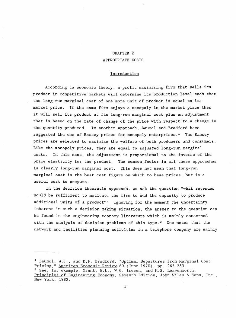
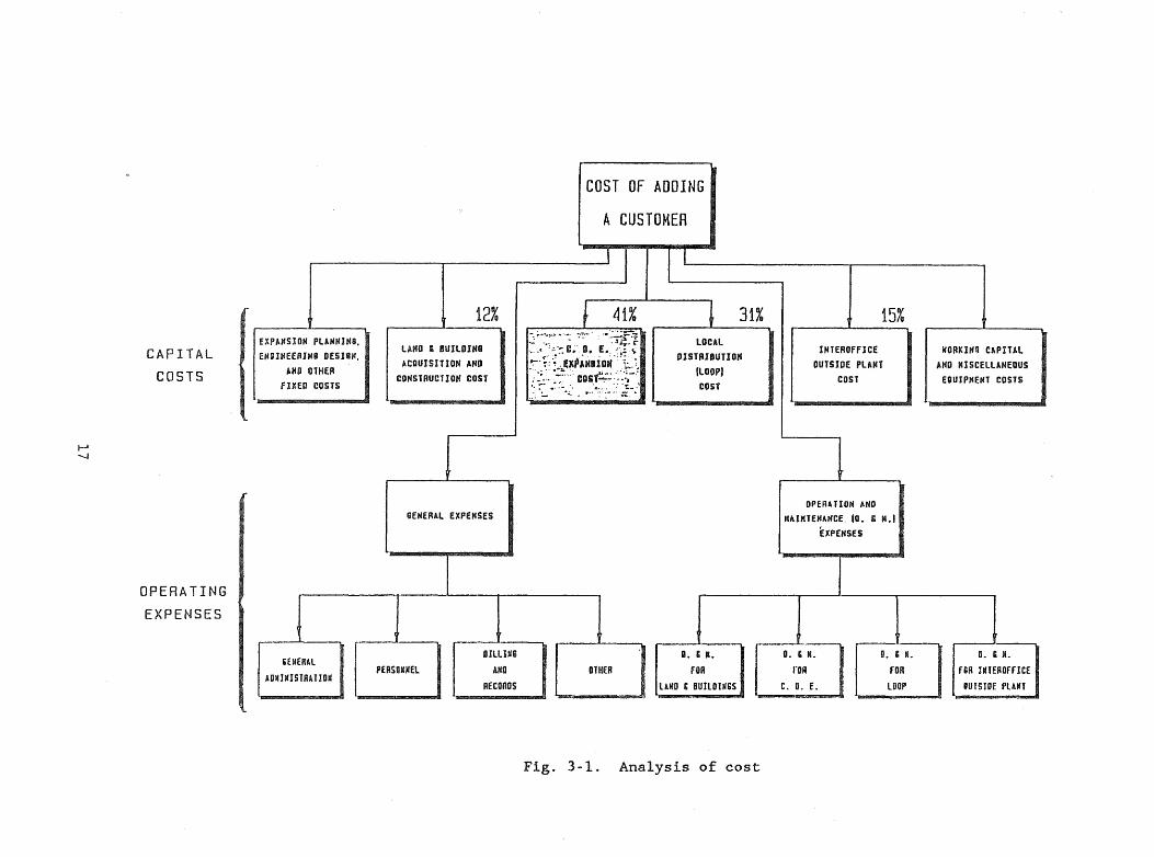
expenses is shown in figure 3-1. We propose a practical method of
determining a total marginal cost that addresses each block in the figure
using an estimation method developed especially for that block. Thus, for
example, one would determine a marginal cost for COE, a separate marginal
cost for loop, one for interoffice outside plant, etc. Assuming these
categories are relatively independent leads to a completely additive model
for combining these costs into a total. If there are any categories where
costs are not independent of others, a different model for combining them
into the total will be needed. For now, it is assumed that the capital cost
categories shown in figure 3-1 have an additive cost structure.
For the present study our attention has been focused almost exclusively
on COE which is represented by the shaded block in figure 3-1. There are
two reasons for focusing on COE. First, of all the system components it is
one of the most difficult to estimate as to its contribution to the marginal
cost of POTS. Therefore, it is the best area to focus research on the
feasibility of ,the approach. Second, the amount of investment in the four
major categories of imbedded plant owned by Ohio Bell in 1985 represented
41% of the total. The other percentages, as shown in fig. 3-1, are
approximately 31% for loop, 15% for interoffice outside plant and 12% for
land and buildings. If we assume that marginal costs will occur in
16
I-' -....J
CAPITAL COSTS
OPERATING EXPENSES
COST OF ADDING
A CUSTOMER
~~~~~~Il-~I--I-~~' ~~~~~~~
EXP~~SION PLA~NINQ.
E"SINEEAIHO OESIS~ AHIl DTHER
fIXED COSTS
I ;[lIEnAL
r""'IRUlOi
I
12%
UNO I: BUILDING ACIlUISlnON "NO
CONSTRUCTIOH COST
GENERAL EXPEHSES
PERSONnEL
ULLING AND
RECORDS
t 41%
f;g~:f1~~~~
OTlIER
31% LOCAL
OISTRJBUUOH IlOOPI COST
II. Ii JI.
fOR
llllO I: BUILDINGS
Fig. 3-1. Analysis of cost
15%
[
INTEROffICE OUTSIDE PLAtH
COST
I '
[
OPERATION AKO "AIHTE~ANCE 10. I: M.I
EXPENSES
I
II. & II.
rOR
C. O. E.
II. 6: II.
fOR
lDIlP
ItORIWf!l CAPITAL AHD MISCELLANEOUS
EIWJPHENT COSTS
D. & It.
f OR INTEROffICE
OUTSIDE PLUT

approximately the same proportions as the present embedded costs, then CaE
is the largest piece of the total. The expansion planning, engineering
design, and other fixed costs are not separately determina?le and are
generally accounted for as part of the investment in plant accounts.
The second largest piece of the total is loop and some attempts were
made in this project to extend our work to loop. However, Ohio Bell has had
an ongoing study of loop costs for well over a year and their
representatives were reluctant to release the basic data gathered in their
study until it is in a final form. As a result, we were unable to obtain
any data relative to loop plant. However, should Ohio Bell's loop study
prove useful for our purposes (and it appears that it will) then
approximately 72% of the total capital costs will have been accounted for in
the two studies. Thus, these two studies address the major parts of the
problem as defined by dollar amounts.
We now present the general method for estimating the contribution of
CaE to the marginal cost of POTS customers.
Cost Study Method for COE
As was discussed in Chapter 1, the typical POTS customer requires an
access line and imposes busy-hour traffic on the system. The busy-hour
traffic is both intraswitch and interswitch if the community has more than
one office. Even when a community has only one office there may be more
than one switching machine in the office. The usual arrangement is to
connect the machine with trunking much like separate offices would be so
that a call from a customer on one switch to a customer on the other switch
involves much of the same type of equipment as would a call across town.
Hence, when we refer to interoffice traffic we also include interswitch
traffic.
The two main customer classes that receive POTS service are business
and residence classes. In our framework, the only significant differences
between these two customer classes are the amounts of the two types of busy
hour traffic they .impose on the system. We shall determine the incremental
cost of adding a number of customers to a switch. With the decision
theoretic framework, such a cost is the threshold value for deciding to
invest in the expansion. However, the incremental cost is expressed as a
18

function of the components of POTS (i.e., access lines and busy-hour traffic
of both types), rather than as a function of the number of customers added.
Procedures are given for then computing the customer cost.
One of the major difficulties with this approach, as mentioned in
chapter 2, is the lumpiness of the investment. It was suggested there that
this would require forecasting the fill rate of new equipment. We also
suggest averaging results over a large number of switches as a means of
minimizing the effect of lumpiness, as well as a means of achieving a
company-wide figure.
From a theoretical point of view, an average marginal cost (or
incremental cost) is not very useful. The reason is that both the economic
theory approach and the decision theoretic approach are based on the idea of
the firm making optimal decisions about its needed capacity. These
decisions are made on a project-by-project basis, and if the service is
priced at the average marginal cost, and if an expansion project is proposed
in an above average cost switch, it would be rejected. However, customers
are not charged differentially if they are connected to different switches.
It is also the case that while a switch may be an above average cost switch
to expand at a particular time, it very well may become a below average cost
switch to expand a second time at a later date. In other words, there is
both temporal averaging of costs of expansions to a given switch and an
averaging of expansion costs across switches. It should be noted that
normal econometric methods of estimating production functions also achieve
average marginal costs. Thus, we believe that as a practical matter
averaging is unavoidable.
The overall philosophy of our study method is as follows: An industry
wide marginal cost is not our goal, nor is it our goal to determine what the
marginal cost should be for a given company. Our view is that in a given
company's territory that company has the "franchise ll to provide service, and
it is their skill and expertise that determines what the service will cost.
Thus, our approach is to use the company as an experimental apparatus on
which we will conduct carefully designed and controlled "experiments" (or
simulations). This consists of having the company engineers develop
expansion plans to satisfy demand scenarios that we specify. These
scenarios are specified in such a way that we are able to estimate the
contribution of access lines, intraswitch busy-hour traffic, and interswitch
19

busy-hour traffic to the cost of the expansion. We then annualize these
costs to determine the annual incremental revenue that is needed to
economically justify the implementation of the expansion plan. These we
will call the marginal cost of the three components of POTS service. Pilot
work with Ohio Bell indicates that these contributions are additive so that
a marginal cost model for any particular customer is easily constructed once
the usage pattern of that customer. is known.
We conclude this section by presenting in step-by-step form a general
outline of the method for experimenting with the company and determining the
marginal cost. This is followed by a brief discussion of the rationale of
these several steps in the method. Following the rationale, a section is
presented in which we examine alternate ways of accomplishing these steps.
Note that each step in the list below is followed by a short title in square
brackets.
1.
2.
3.
4.
5.
6.
7.
Select a sample of switches.
Establish an ESS lA equivalent switch design for the non-ESS switches in the sample.
Have the company design expansions for the sample switches according to an experimental plan.
Organize the equipment lists for the expansion plans and examine for inconsistent patterns -- request revised designs when needed.
Fit a spline function regression model to four different sized expansions.
Compute an average annual unit cost for each output variable.
Compute an average annual cost per customer for residential and business customers.
[Select sample]
[Standardize technology]
[Design expansions]
[Audit designs]
[Analyze]
[Average]
[Compute]
It should be noted that step 2 is an Ohio Bell specific task. If the
company under study is not Ohio Bell, the technology to which all switches
in the sample should be II s tandardized" is the predominant modern technology
for that company. Step 3 also deserves comment in that, for Ohio Bell it is
20

a relatively easy step to perform because of the availabililty of a
computer-aided design package for its lA ESS switch. It is assumed that
other companies have similar design aides that will facilitate their
performance of step 3.
Method Rationale
Before proceeding with details of the steps of the method, it is
appropriate to discuss the rationale for the several steps of the method. -
Among the first five steps, steps 3 and 5 are key to the problem. These two
steps have the goal of establishing, for each switch in the sample, a
relationship between variables that define POTS customers' demands on the
system and the cost of expanding an office in order to satisfy that demand.
In our case here, a POTS customer, as defined in chapter 1, is represented
by a vector of demands with components consisting of a line (Xl)'
interswitch busy-hour usage (x2 ), and intraswitch busy-hour usage (xs )'
The non-operating cost of an expansion built to serve a POTS customer
consists of all cash flows associated with expanding the switch. This
includes one time expenses to cover removal and rearrangement of existing
equipment items, and the installation of additional equipment items.
Because these cash flows have components that receive different tax
treatments we seek to establish the relationship mentioned above separately
for capitalized and expensed items. We designate these two components as
capital costs (y ), and expansion related expenses or simply expenses (y ). c e
Total cash flow at time zero is designated Yt and and is related to its
components by the relationship: Yt= y + Y , where we have made the e c
simplifying assumption that all expansion cash flows occur at one point in
time designated as time zero.
Because of the relationship given immediately above, only two of the
three cash flows Yt' y , and y need to be modeled in steps 3 and 5. For e c
purposes of exposition, the ideal relationship established by steps three
and five would take the form:
(1)
(2)
21
where ai' and b i are model parameters established by the method. The
marginal cost of adding a customer with, for example, one line, one
intraswitch busy-hour CCS of use, and three interswitch busy-hour CCS of use
would be the vector product:
(3)
The vector product,
(;) \1/
(4)
is needed only to transform the one-time lump-sum marginal cost in (3) into
an annualized rental rate.
Unfortunately, one cannot expect actual cost structures to be as simple
as (1) and (2). Instead, in a preliminary part of this study, it seemed
that costs for the different components of POTS interacted with one another
as well as with other non-POTS variables such as DID trunks (x4 , which also
acts as a proxy for DID trunks). The results suggested the possibility of
interaction of some POTS variables with.interexchange busy-hour CCS (xs ) as
well. Furthermore, there are fixed costs associated with expansions, and
due to lumpiness of equipment, costs depend on the size of the expansion and
the present state of the office being expanded. The effect of the size of
an expansion on its cost is dealt with by developing four cost models rather
than just one. Each cost model represents the costs of one of four
differently sized expansions. The effect of the present state of a switch
could be treated by constructing a cost model for every switch the company
owns. This approach would be enormously expensive and time consuming. This
is the reason a sample of switches is chosen in step 1 of the method. The
sample should, of course, be representative of the popUlation of all
switches.
Interactive effects on costs and fixed costs require a more complex
function to reflect the cost structure. The form these models now take is
as follows:
22
Yts aOs + a ls xIs + a 2s x 2s + ... + aSs xSs + a12 ,s xIs x2s
+ a l3,s xIs x3x + . . . + a IS,s xIs xSs + ...
+ a 45,s x4s xSs
for lIs oS x. :S u. ; i 1, ... , 5 . and s 1, • " lit , 4 (5)
~s ~s ,
Ycs bas + b ls xIs + b 2s x 2s + ... + b Ss x5s + b12 ,s x. x2s ~s
+ b l3,s xIs x3x + . . . + b x 15, s_ Is xSs + ...
+ b /. c: X /._ xc:_ .... ..;,5 .... :::; ..;:::;
for 1. :S x. :S u~s ; i-I, ... , 5; and s = 1, ... , 4 ~s ~s ...
(6)
where the subscript s indexes the model and variables for a size s
expansion, and where aOs' bOs are intercept terms that represent fixed costs
when s = 1. Terms such as a13 ,s and b45 ,s are the coefficients for two
variable cross product terms. These models could each include up to 10 such
crossproduct terms. Finally, 1. and u. are lower and upper bounds giving ~s ~s
the ranges of variable values over which the size s expansion is defined.
The important finding of our examination of the specific nature of
functions (5) and (6) for the one switch studied in the pilot is that only
four cross-product terms in all eight models and only one of the two fixed
cost terms are different from zero. The four cross-product terms that were
nonzero always involved x2s (interswitch busy-hour CCS) and x4s (DID
trunks). Two of these terms were present in size 1 and size 3 versions of
the total cost models (equations 5) while the other two were also size 1 and
3 versions of the capitalized cost model (equation 6). The fixed cost term
was nonzero only in the total cost model, indicating that it results mainly
from expense type items. Once the nonsignificant terms in these models are
eliminated, they become nearly as simple as the ideal models given in
equations (1) and (2). The lack of any cross-product terms that include Xs
(interexchange busy-hour CCS) implies an additive switching cost structure
between POTS and toll services. This allows Xs to be held fixed for the
experimental plans as proposed for step 3.
23
The analysis procedure used to establish the models in step 5 was to
treat the four size models as four segments of a spline function and
estimate all parameters simultaneously with constrained least squares. This
approach permits one to accurately model the observed data points while
retaining a simple mathematical structure for each size range. In reality,
these models should not be viewed as having some theoretically justifiable
structure; instead, they may be viewed as models to interpolate at points
between actual observations. These interpolation models fit the actual
observations extremely well, which cannot generally be said fo.r ordinary
regression with a single given model form.
The audit step (step 4) is, of course,
are received in response to a data request.
for face validity will often reveal errors.
always necessary whenever data
An examination of a response
In the case of this study, the
balance of experimental design used in the data request provides a way to
organize the data in order to greatly strengthen a face validity test.
Step 2, the calibration step, is needed to make the expansion planning
process begin with a switch which conforms with the switch in the actual
office. The conformance is with respect to the current status of demand and
capacity at the sample switch. The conformance with respect to technology
is not necessarily achieved unless the expansion planning process can be
done on any variety of switch for all the experiments that are requested in
step 3. At Ohio Bell, only the 1 and lA ESS switches could have expansion
plans developed and costs estimated by a computer aided design package.
Without such a package the response to step 3 may impose unduly high study
costs on the company. There is even some doubt that calibration of a non
ESS switch is a practical step. If it must be avoided, step 1 may be
modified by selecting the sample from only the switches with the qualifying
technology.
Steps 6 and 7 use the cost models developed in steps 1 through 5 to
compute an estimate of the company-wide annualized marginal cost of a POTS
customer. Since the cost function of an expansion is dependent on its size,
the first question is how large an expansion should be assumed. In one
sense, the larger the better, since this allows averaging lumpiness of
investment over a greater number of units, thereby mitigating its effect.
However, building a large expansion may create excess capacity for a
significant period of time (depending on growth rate) and thereby cause an
24
overestimation of marginal costs. This is where demand forecasts have their
direct effect on the estimate of marginal costs. Given these demand
forecasts these steps seek to determine how large an expansion should be
where the annual equivalent cost of the expansion is minimized on a per line
basis. This should represent a reasonably good economic sizing of the switch
expansion.
Thus, a cost model is determined for each office in the sample in steps
1 through 5 and averaged in step 6 using a weighted average calculation.
These cost models are then converted to a per customer cost (depending on
customer class) in a fashion similar to the idealized calculations shown in
equations (3) and (4). The weighted average referred to above weights each
cost model with the probability that a customer will join the corresponding
office. This provides a means of recognizing that the actual costs incurred
with growth in customers is very much a function of which offices actually
need expansion, and not just a simple average of expansion costs.
The next section will discuss in detail each of the steps listed
earlier. Many of the details are appropriate for Ohio Bell where computer
aided design is routinely used. Also included are evaluations of
alternative methods of accomplishing these steps.
Detail Analysis of Steps
Step 1: Select sample
All switching machines owned by the company within the Ohio
jurisdiction should be available for possible selection into the sample.
The purpose of the sample is to provide the objects on which an experimental
plan will be implemented so as to obtain a company-wide estimate of the
marginal costs of access lines and local usage. Two basic sampling methods
are considered:
1) random sampling, and
2) stratified random sampling.
The first of these, random sampling, is the simplest and is performed
by selecting switches one-by-one in such a way that each switch has an
equally likely chance of being selected.
25

The second plan, stratified random sampling, divides the population of
switches into groups called strata and allocates a certain portion of the
entire sample to each stratum. Each within-stratum sample is then drawn
randomly as described above. Stratified random sampling has a benefit when
the switches can be grouped into strata in such a way that the
uncontrollable factors which influence the cost of expansions occur in a
relatively homogeneous fashion within each stratum. Since our empirical
work involved only one switch, we can only speculate as to how one should
stratify the Ohio Bell switches. The leading candidate criteria for
defining strata would have to be whether or not the switch is found in a
single switch exchange, and whether or not the population surrounding the
switch is growing rapidly, slowly, not at all, or decreasing. Another
reasonable candidate might be the number of access lines.
One can achieve a significant benefit from a stratified random sampling
plan only if some estimate of the within-stratum variance is available.
Such knowledge would permit an "optimal" allocation of the sample size to
each stratum.
Step 2: Standardize technology
A random sample of switches is likely to contain switches with several
different switching technologies. Some of those technologies may be quite
outdated in that they are not the technology of choice in present day
practice. Examples are step-by-step and crossbar. When such switches need
more capacity a number of design alternatives may be considered that avoid
increasing the investment in the older technology. The only case in which
the older technology would be selected is when it is economically
competitive with solutions using the new technology. We assume that is
roughly equivalent (on a marginal cost basis) to replacing the switch with
the newer technology and then expanding that new switch. Therefore, when a
sample switch employs an outdated technology, this step asks the company
engineers to design a replacement switch that would use the newer
technology. This ilhypothetical li switch should have the same service
characteristics as the real switch, and it will replace the actual switch in
the sample of switches that were selected in step 1.
26
Since the sample switches are the ones that will be used to estimate
expansion costs, the disadvantage of the standardization process is that it
minimizes the range variation likely to be found. The purpose of this
standardization is to be able to take advantage of the computer aided
design packages that are readily available for switches that use the ESS
equipment. This greatly reduces the cost of the data and increases
reliability and consistency of results. One might also argue that costs
that are related to present day technology are the only costs relevant to
present day decisions. An alternative to this standardization step would
corne from modifying step 1 so that the universe from which the sample is
drawn would include only 1 and lA ESS switches. This would obviate the need
for step 2.
Step 3: Design expansions
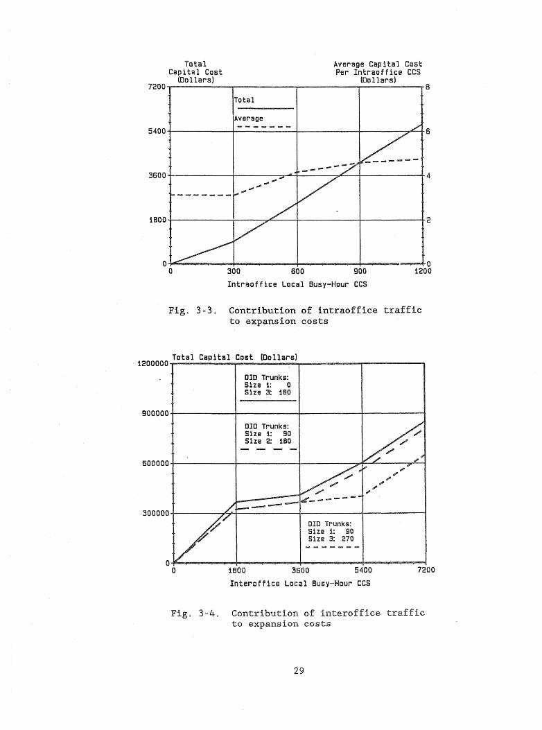
The cost of expanding each switch in the sample must be investigated in
much the same way as has been done in the pilot work of this project. The
type of results to be obtained for each switch is depicted in figures 3-2
through 3-9. These figures give the results that were obtained in the study
of one Ohio Bell switch. In that study there were five variables used to
describe an expansion. These variables were: access lines, intraswitch
busy-hour centrum call seconds (CCS), interswitch local busy-hour CCS,
direct inward dial (DID) trunks, and interexchange busy-hour CCS. Four
different sizes of expansion were considered, and within each size two
levels of capacity additions in each of the above variables were considered.
The four sizes are designated size I through size 4, and an analytical model
was fit to the data from each size. The reason for including in the study
the two variables that do not pertain to POTS, i.e., DID trunks and
interexchange busy-hour CCS, was that we were concerned with the possibility
of a joint effect on cost of these variables with those that do pertain to
POTS. Such joint effects turned out to be virtually non-existent. The only
joint effect of significant magnitude was a cost savings that occurred when
both interswitch local busy-hour CCS and DID trunks are added to the switch
simultaneously. This joint effect occurred in the size 1 and size 3
expansions but not the size 2 or size 4 expansions. As a general rule, one
27

cannot predict which size expansions will exhibit this joint effect because
it is dependent on the existing structure of the switch being expanded, as
well as on the size of the expansion.
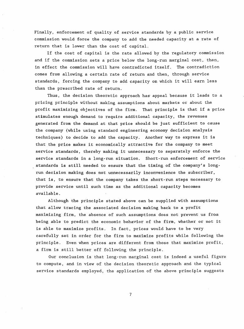
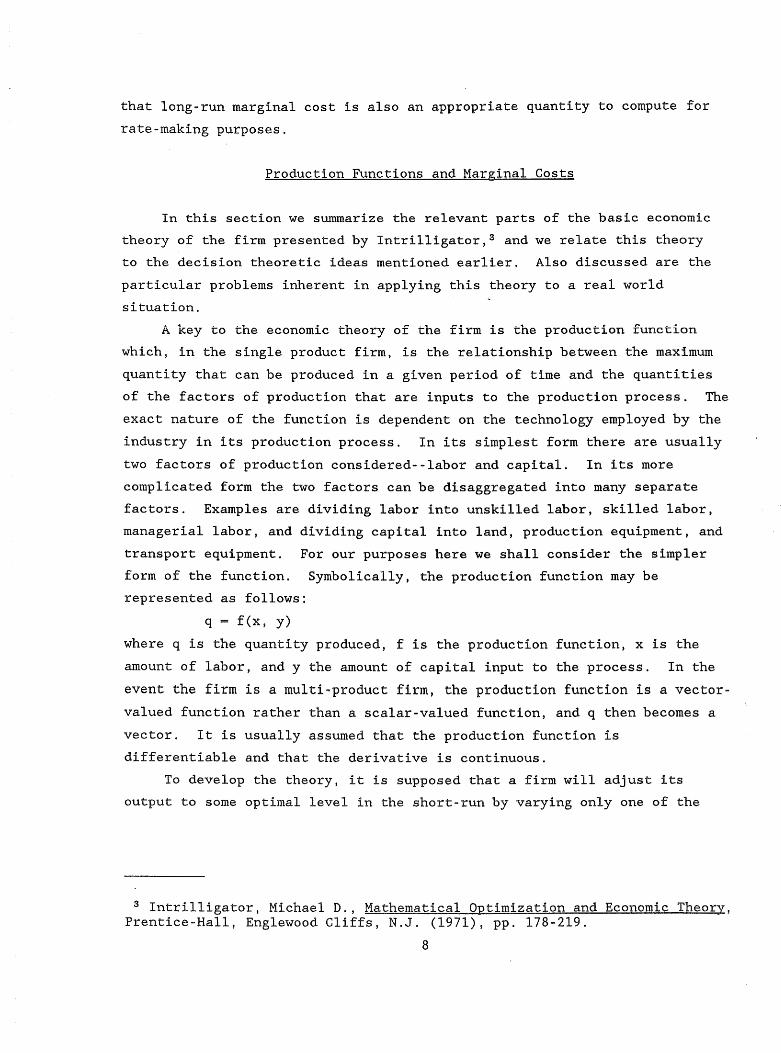
Figures 3-4, 3-5, 3-8 and 3-9 show the effect of the joint cost savings
on both the total cost, capital cost and the average costs when the entire
benefit of the joint cost savings is allocated to the interswitch local
busy-hour CCS.l
Total Capital Cost
(Ool1arsj
Average Cap ital Cost Per Line
(Dollarsj 20000?----..--------F---------~------------_r----------~20
I
15000~--------------+-------~/~/-+------~~-+~~----------~i5 I
I I
I I
iOOOO~--------------~----T_----~_4----------_+----------------~iO
Average
5000+---------------~~~----_4----------------_+------------------~5
O~~--------~--------~----------_+--------~~O o 350 700 1050 1400
Access Lines
Fig. 3-2. Contribution of access lines to expansion costs
1 The issue of how much should be allocated is more a pricing and/or policy question than it is a cost study question.
28
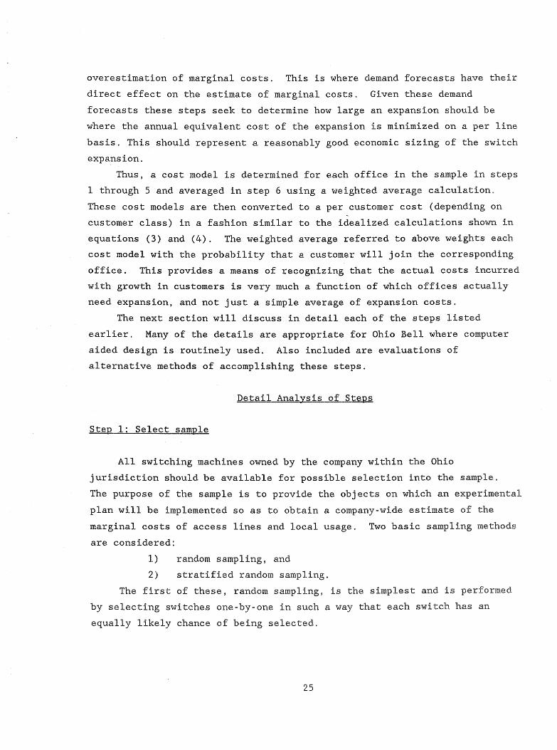
Total Average Capital Cost Capital Cost Per Intraoffice CCS
(Dollars) (Dollars) 7200~--------~~--------~----------~----------~8
Total
Average
5400+-----------+-----------+-----------~------_7~6
3600+-----------+-------~~+-----~~--~--------__+4
1BOO+-----------+_----~----+_----------~--------_+2
Intraoffice Local Busy-Hour CCS
Fig. 3-3. Contribution of intraoffice traffic to expansion costs
Total Capital Cost (Dollars) i200000~-----------~~--------~----------~--------~
DID Trunks: Size 1: 0 Size 3: 1BO
900000+------------+_-----------~----------r_--------_4
Ole Trunks: Size 1: 90 Size 2: 180
600000+---------~~--------_4--------~~~----~~
300000+-------~~~--------_4----------~--------~
1800
DID Trunks: Size 1: 90 Size 3: 270
3600 5400
Interoffice Local Busy-Hour CCS
7200
Fig. 3-4. Contribution of interoffice traffic to expansion costs
29

240 Average Capital Cost Per CCS (Dollars)
DID Trunks: Size 1: a Size 3: 180
~
~'~ OlD Trunks: Size 1: 90 Size 3: 160
...- - - -"
180
120 - -- -~ - - -....... ... ............ ------.... _-60 -
DID Trunks: Size 1: 90
a 1800 3600 5400 7200
Interoffice Local Busy-Hour CCS
Fig. 3-5. Average interoffice traffic contribution to expansion costs
Total Cost (Dollars)
Average Total Cost Per Line
(Dollars) 20000~----------~--------~------------r----------~20
I .... I ....
1S000 I is I I
I I
I I
10000 10 Total
Average """*------
5000 5
O~~------~----------~----------~---------+O a 350 700 1050 1400
Access Lines
Fig. 3-6. Contribution of access lines to total expansion costs
30

Total Cost (Dollars)
Average Total Cost Per Intraoffice CCS
(Dollars) 7200~----------~--------~-----------r----------~B
Total
Average
5400+-----------+-----------+-----------~~~------+6
3600 +--------+-----."..:;---+---:::J.c-----+------__+ 4
1BOo+-----------~--~~---4----------~----------~2
O~~--~~--~--------~----------~----------~O a 300 600 900 1200
Intraoffice Local Busy-Hour CCS
Fig. 3-7. Contribution of intraoffice traffic to total expansion costs
Total Cost (Dollars) 1200000T---------------------~----------_F--------__,
DID Trunks: Size 1: 0 Size 3: 180
900000+-----------~---------4----------~--------~
DID Trunks: Size 1: 90 Size 2: 180
600000+-----------+-----~----+_---~~--~-----~~~~ ~
~ ~
~
.------ ~
300000+-------~~~--------_4----------~--------__;
1800
DID Trunks: Size 1: 90 Size 3: 270
3600 5400
Interoffice Local Busy-Hour CCS
7200
Fig. 3-8. Contribution of interoffice traffic to total expansion costs
31
280 Average Total Cost Per CCS (Dollars)
DID Trunks: Size 1: 0 Size 3: 180
140
'" ~---
'~ OlD Trunks: Size i: 90 Size 3: 180
" - - - -" '- -
210
,~ .::- ...... - -- -- -- -........ - --~ ........ ---------..... 70 -
n'?n ,.~ .. _ ... _.
Size 1: 90 Size 3: 270
I I
UJ.U II UIlI'i.::'U·
o-+--~~~---~----o 1800 3600 5400 7200
Interoffice Local Busy-Hour CCS
Fig. 3-9. Average interoffice traffic contribution to total expansion costs
The fact that most joint effects on costs are not present is a
desirable result because it indicates that the cost structure is relatively
simple. The simplicity is evident when one compares figures 3-2, 3-3, 3-6
and 3-7 with the other figures. This result also means that a simpler
experimental design can be used when the method is applied to a sample of
several switches. In the pilot, 16 experimental observations were necessary
to examine the individual cost effects and the joint cost effects of the
five variables. These 16 observations yielded 64 data points that were
separated into 4 sets of 16 points each in order to establish a model of
each of the 4 size expansions. Thus, 64 data points are actually necessary,
but only 16 experimental runs are needed to obtain the 64 points because of
the inherent features of the computer aided design package being used and
because of our ability to take advantage of those features in the
experimental plan.
When the method is applied to a sample of switches, the interexchange
busy-hour CCS variable can be eliminated (held fixed at value zero) since it
is not a POTS variable and since it has no interactive effect on cost with
32
the POTS variables. Unfortunately, DID trunks cannot be similarly
eliminated. However, elimination of the one variable reduces the number of
data points needed to 32 from 64 and consequently reduces the number of
experimental runs to 8 from 16. The resulting experimentation plan is given
in appendix B in the format used in the pilot study. This is referred to as
a 24
- 1 fractional factorial design (each of the 4 sets of 8 points result in
such a design.)
A second experimentation plan is given in appendix C. This plarl
achieves a further reduction in the number of experimental runs needed by
essentially eliminating the DID trunk variable. In this case, we do not
fully experiment with the DID trunk variable so that its effects cannot be
measured, but we also do not hold it fixed to value zero. Instead, 45 DID
trunks are added in all size 1 expansions, and that value is increased by 90
each time we shift to a new size. Since the DID trunk variable is not
varied within each size, the number of required data points is again reduced
to 16 from 32, and the number of runs needed to obtain those points is
reduced from 8 to 4. The effect of this approach is to pass all of the
savings that result from the joint addition of DID trunks and interswitch
busy-hour traffic on to the interswitch busy-hour traffic variable. While
this seems inequitable, it must be remembered that, if in reality many more
DID trunks are added than were assumed in the experimental plan, more actual
savings would occur than would be accounted for. The model would allocate
all the accounted for savings to interswitch busy-hour traffic and those
savings not accounted for would be left to the DID trunks. Thus, a form of
sharing would take place.
Our recommendation is that in initial studies the 8 run
plan be used so that a more precise picture of the interaction between DID
trunks and the interswitch traffic can be drawn. This will allow a
procedure to allocate the cost savings according to a reasonable
rather than being hidden in the mathematics of a model. Once it is learned
how to make the mathematics of the model accomplish the same allocation that
would be made if the principle was applied, one could use the
plan in appendix B and reduce the data
study method.
33
and the cost of the

Step 4: Audit designs
Once the telephone company engineers have designed the expansions for
the sample switches, it is necessary to examine the results for ertors or
inconsistencies. While we cannot expect to be able to discover all errors,
we can discover results that do not appear to make sense. This type of
reasonableness check is facilitated by the fractional factorial experimental
plan that defined the expansions to be examined. These plans are known for
balance and symmetry so that when the data are systematically organized in a
particular format, one can examine for balance and symmetry in the expansion
designs developed by the company. ~~en there is imbalance and as}~T.etry
noted, the company can be asked for an explanation.
In the pilot study this process was very effective and proved to be an
essential step in the acquisition of reliable data. The results of the
pilot study will be used to illustrate the audit process.
In factorial experiments there is an ordering of the observations that
is referred to as the natural ordering. Arranging fractional factorial
observations into a natural ordering is a bit more complicated but is always
possible. 2 The designs we recommend consist of four different sized
expansions, with each size incorporating a series of expansions in which
each variable assumes one of two values--called a high level and a low
level. An observation within a given size expansion is then designated with
a lettering system employing lower case letters to represent each particular
variable. For example, in our pilot work "aU stood for access lines, lib"
for DID trunks, "c" for intraswitch busy-hour CCS, lid" was interswitch local
busy-hour CCS, and "elf represented interexchange busy-hour CCS. The
lettering system referring to a particular combination of variables that
corresponds to an observation uses a letter to represent each variable that
is at its high level, and excludes letters for variables that are at their
low level in the observation. Thus, for example, Ita" refers to an
observation in which variable "a" is set to its high level and all other
variables are low, and "abel! denotes an observation in which variables "a,n
2 See for example, Montgomery, D.C., and E.A. Peck, Introduction to Linear Regression Analysis, John Wiley & Sons, 1982.
34
lib," and "e" are at their high levels while IIC" and "d lt are at their low
levels. (1) is used to denote an observation in which all variables are at
their low levels. Because of the experimental plan specified for each size
expansion, the all high observation, abcde, for one size is exactly the same
observation as the all low observation, (1), for the next larger size.
The natural ordering for a full factorial involving the five variables
listed above is as follows: (1), a, b, ab, c, ac, bc, abc, d, ad, bd, abd,
cd, acd, bcd, abed, e, ae, be, abe, ce, ace, bce 7 abce, de, ade, bde, abde,
cde, acde, bcde, abcde.
Our experimental plan was a one-half fraction of the above plan and has
the natural ordering as follows: e, a, b, abe, c, ace, bee, abc, d, ade,
bde, abd, cde, acd, bcd, abcde. In this one-half fraction, the all low
observation is not part of the plan but'the all high is included. Even
though the all low is not part of the design for a given size, it is
available as the all high observation in the smaller size, since adjacent
size expansions have the all low and all high observations in common. The
size I expansion has, by default, the all low observation available as well,
since it represents no expansion at all and, therefore, has no cost and no
equipment added.
It is this natural ordering that is the systematic format needed to
examine the data for errors. Tables 3-1 through 3-4 show, respectively, a
matrix of equipment numbers for the size I through size 4 expansions. Each
column represents a particular expansion plan described in terms of the five
variables listed at the top of the column. The first five rows of these
tables give the actual amounts of increased capacity in the expansion. The
sixth line gives the factorial letter codes for the observation (expansion).
Note there are a total of 16 expansions for each size and all are displayed
in the corresponding table in the natural order from left to right.
The main bodies of these tables contain the number of items of equipment, by
type, that would be deleted or added in an expansion. The bottom rows of
the tables give the capital costs and the total costs of the various
expansions in thousands of dollars.
There are very recognizable in the of
the numbers in the main body of table 3-1. Similar are found in
the main bodies of tables 3-2 through 3-4, but they are much harder to
recognize. For that reason, tables 3-5 3-7 were created by
35
subtracting the amounts of equipment needed for the all low expansions for a
given size from the equipment lists of all expansions in the size. These
new tables for sizes 2, 3, and 4 now appear very similar to table 3-1 for
size 1, where the patterns in the numbers of equipment are more easily
recognized. The audit process consists of examining for breaks in the
patterns, or unexplainable shifts in the patterns. The two cost rows are
included in this examination. To consider a specific case, table 3-8 has
been constructed to simulate several of the situations encountered during
the pilot study. Some of these situations required new expansion plans from
the telephone company. Table-to-table comparisons should also be made. In
table 3-8, areas of the table have been circled where questions of validity
of the data should be raised.
In addition, an examination of the costs in table 3-8, which are
actually incremental costs between size 2 and size 3 expansions, reveals an
inexplicable shift in cost. For example, the "e ll expansion in table 3-8
differs from the ilabcde" expansion in size 2 by only a few more small items
of equipment and yet the costs are significantly higher. It was discovered
that errors had been made in several size 3 expansions. Comparisons across
tables 3-1, 3-5 to 3-6 show a jump in costs when interswitch busy-hour ccs capacity is added in size I and size 4 expansions but not size 2 and size 3
expansions. This particular result was not an error and could be explained
by the addition of a very "lumpy" piece of equipment in the size I and size
4 expansions. s That equipment was a line-link network (LLN). A small LLN
was first added in the size 1 expansion with no change in the size 2 and
size 3 expansions, but it was replaced with a larger LLN in the size 4
expansion.
Finally, we found that an electronic spreadsheet, such as Lotus 1-2-3,
was an excellent tool to organize the data as described above. Other
techniques were tried, such as numerical analysis of the equipment lists,
but were found to be no more effective than the simpler pattern-recognition
technique.
3 In the study we were given the description of the equipment added under a protective agreement. In the tables we have expunged the equipment names to prevent revealing what Ohio Bell considers to be proprietary data.
36
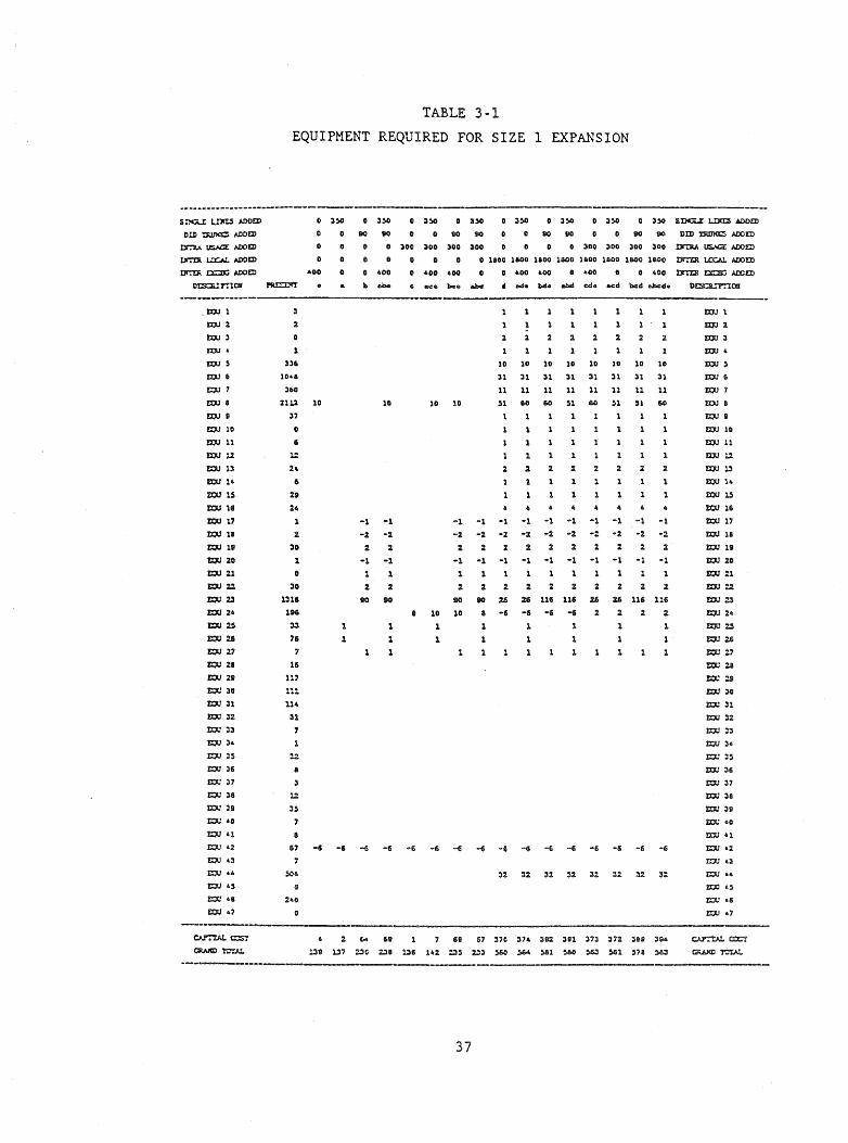
s ~ lnrtS ADDED
DID ':]1.11I(CS ADOfl)
tr.'1l.A u:.s...a AOOfl)
Ir.Di. ~ ADDC>
tr.'C\ tx::lJj ADD£:)
TABLE 3-1
EQUIPMENT REQUIRED FOR SIZE 1 EXPANSION
o 3)0
o o
400 0
o 3)0 (I 3 ~ S DG...E um:::s A.OOfl)
110 110 DID nuna::s AOOC>
)00 300 )00 o )00 300 300 300 o 300
o o 1II0C 1500 11100 1&00 11100 1&00 1500 111100
o 400 400 o "00"'00 11 .. 00 0 400 nrn:R c::::lJIj A.DC1:ll
D~rnOll ~
o 400
Ii> ..0.. III ...:I.. We mbd eel.. ....d bed a.bc:d.. DCSO"n''':'lOlill
. tOJ 1
tOJ a tOJ 3
tQU 6
EClI 5
tOJ Iii
~ 7
EClI 8
EClI Il
£OlI 10
rcu 11
J:X)U U
£OlI 13
J:X)U 14
J:X)U 15
£OlI 16
J:X)U 17
&QU 111
J:X)U 19
&QU 20
E:IU :1 E:IU 22
&QU 2!1
CJU 2"
CJU :s &QU 215
E:IU :7 E:QU 211
f1JIJ 211
t::lC 30
f1JIJ 31.
E:QU 3: CJU 33
EClI 3.
rou :!s !:.lIJ 36
rr:x: :17
E:IU 38
£OlI 39
t::IU 60
EClI 41
EClI 42
mu 43
mu u
£OlI 6S
rr:x: .e £OlI 167
336
10-.
360
:UU
37
o 6
1.:
2,
.. :9 24
: 30
1
16
117 1!1
11"
31
7
1.:
:IS
7
II
10
1
10
-1 -1
-2
: -1
-: 2.
-1
1
Z
to
1
1
1
1&1 10
1.
2
1
:t
1
2.
1.
10 10 10 10 10 10
31 31
11 11 51 60
31 31 :n 31
11 11 11 11
60 51 60 51
1 1 1
1
1
2 :t
1.
1
-2 -:
:: 2
-1 -1
1 1
2 2
90 26
8 -6
1
-: -2 -:
Z 2 ::
-1 -1 -1
1 1
:% :%
26 116 116
-6 -6 -f!
1 1
1
1
-: -: -: -2
:% 2 2
-1 -1 -1
1 1 1
% : :I
26 116 116
:: 2 2.
1 1
1 1
1 1
» ~ ~ ~ ~ ~ ~ ~ ~ ~ ~ ~ ~ ~ ~ ~ ~
::: "" 6111 Ii II 67 3'Il 374 3sa 391 )7:1 372 :111111 )1).4
!.3f1 1.:17 ~C ::Iii 1.:18 14: :::IS :t:l) :!6Il 564 51111 $&0 :,I.tI.:I 561 578 )a:I
37
toU 1
IlJO 2
IlJO 3
IlJO •
IlJO 5
roJ 6
IlJO 7
tOJ II
tOJ II
toU 10
EClI 11
EOU 1.2
EOU 13
EOU 14
tOJ 13
EOU 16
rcu 17
tOJ 11
EOU 19
tOJ :0 EOU :1
EOU :.:t Et.1l1 :3
£OlI 2'
EOU :s tOJ .:a IOU =7
IOU 2JI
EtC :lI
EOU 30
rr:x: :ll
tcU :12
tcU ~3
t::JIJ 3.
t::JIJ :!S
toU 36
r::::c.J 37
mt: 31
Et.1l1 :lSI
rr:x: 60
EOU 41
rou 42

TABLE 3·2
EQUIPMENT REQUIRED FOR SIZE 2 EXPANSION
-----------------------------_.------------------------$:!G...l um::s ADDED
D Ul 'Olma:s ADDED
t-vnv. USAGE ADDED
3~ 700 3)0 700 3)0 700 3~ 700 3~ 700 3~ 700 3~ 700 3~ 700 S'l.'G.L um::s ADID!l:I
eo 90 lao lAO 110 IilO 180 lAO 110 90 110 1&0 eo 110 1110 180 DID tJ!llICICS A.DOm
300 300 300 :)GO 6(10 1100 &00 600 300 300 )00 300 6(10 iOO &00 .00 :tr.:lIA USIa ADDm
~ t.OC.t.!. ADDED 1&00 1100 1800 11Il00 1800 11Il00 1800 11100 3600 3600 3600 :J.oo 3600 3600 )&00 3600 IJr':l:ll lJX..tJ. ADDED
tJr:'"£i\ c:::::I!G AOOC> 800 400 600 800 400 800 11"0 600 400 800 800 liDO 1100 400 400 800 IJr':l:ll:oc::llC.wem
Dts::IUr."lOli rru:::;::orr iii abe C .... Of)c... eba: d...d" W. No4 eel. _01 bed &bed. Dt:s:::Il.ll":'
too 1
lOU :I
lOU 3
too 4
too ,
roo &
roo 7
too e too
too 10
r:ou 11
too 1.:
too 13
too 14
mu 15
mu 16
too 17
too 18
too 111
too 20
roo n roo .u roo 23
too 24
mu ~ EQU :u;
too 27
too 211
too 2S1
roo 30
too 31
too ::Ill
too 33
too 34
rou :IS
too :31, too 37
to:: 31
too Jill
too "0
too 41
too 42
EOU 43
rou 44
too 4S
too 4' too 47
360
:u.:.:t 37
10
:U 11
70
1
2
10
:)1
11
.0
2
1
2
1
10
:n. 11
f50
2
1
10
31
11
70
1
2
2
1 10
31
11
60
: 1
:1
1
10
31
11 70
a 1
10
:n 11
70
:1
1
1
2 2
1
2
1
10 20 20 20 20
31 63 63 63 III
1.1 .u :tl :.2 :.:l
60 111 121 121 111
1
1
2
2 2 2 2
1
:&
1
2
2
1
l
1
2
1 1
:t :t l
1 20 20 20 20
6J 63 6J 63
:tl :.2 .u .u 1.:1 111 111 121
2 2 l
1 1 1
2
1
:
2
1
2
2
1
2
:t
1
2
-1 -1 -1 -1 -1 -1 -1 -1 -1 -1 -1 -1 -1 -1 -1 -1
2 -2 -2 -2 -2 -2 -2 -2 -2 -1 -2 -2 -2 -2 -2 -2 -a 30 2 l 2 a :: a 2 2 :: 2 :. a 2 2 2 2
-1 -1 -1 -1 -1 -1 -1 -1 -1 -1 -1 -1 -1 -1 -1 -1
01 1 1 111 1 11 1
30 2 2 : 2 : 2 2 :. 2 2 2 2 2 2 2 2
1318 116 111 206 206 116 115 206 206 111::1 143 233 233 143 143 233 233
1S1S 2 2 10 12 12 10 6 II 6 6 14 14 14 14
~ ~ ~ ~ ~ ~ ~ ~ ~ ~ ~ ~ ~ ~ ~ ~ ~
76 fI 10 III 10 II 10 II 10 10 10 10 II 10
, 1 1 1 1 1 1 1 1 1 1 111
16 2 2 2 2 2 2 2 2
1:'7 ::\ ::\ :I
1~ :I :I 3
l.~oto l. l. 1
31 -z -1 -1 -2 -a -:t -a -2 -% -2 -Z -2 -Z -: -: -lL
'l
-8 -II
-e -CI
-II
-6
-ID -a -a -I -I -a ~ -I ... -I -i ...
1101 '07 618 1.:31 :IN 411 42,3 621 43111 4:11 46.3 469 .'3 449 _60 47:1
S9C :196 608 I!I2C s,u 601 61.2 1111 I!I2Jl 641 ISs.: II~ 632 6311 6~ 66:t
38
11;10 1
11;10 2
11;10 3
J:OO •
11;10'
WJ II
11;10 7
11;10 II
WJ II
EQO 111
WJ 11
11;10 :.:z J:OO u J:OO 14
11;10 U
J:OO 15
J:OO 17
Il:lO 111
J:OO 111
J:OO 2U
Il:lO 21
J:OO n J:OO :3
Il:lO ::toto
11;10~
1:002.5
EtC V
Il:lO :t.I
D:IC 2S
Il:lO 30
r:cu :'11
Il:lO 32
WJ 13
WJ 3.
JXI1 :,
J:OO 35
D:IC 37
D:IC 311
r::JO ::It
r.tl1~
WJ 61
JJ::X1 1.2
11;10 .. 3
IJ:jlJU
11;10 to' !CO ~
Et)!.; .. 'I
S L'G..t LDtI:S ADOm
DIn llUl!O:S ADOm
tJmi.A. I.lS.A.GE ADO£:!)
lJITDl ~ ADO£:!)
IJrl"tIi c:oo ADOI'J)
DE:SCILIl"rIOlll
WJ 1.
WJ 2
WJ ;)
D:JU ..
D:JU 5
WJ 6 WJ ,
D:JU 8
WJ II
D:JU 10
D:JU 11
EOU 12
D:JU13
D:JU 14
EOU 1.S
:tQU 115
WJ 17
tOU 111
tOU 19
E:l:)U 20
WJ 21
WJ 2.%
WJ %3
WJ 24
J:OJ U
tOU 26
l':J\l 27
tOO 28
tOO 29
tOO 3D
!Xlt1 ::11
t::7J :12
WJ :13
tOO 34
l':J\l :15
tOO 36
t::U ::17
WJ 3. t::U :III
tOO .0
tOO 41
l':J\l 42
tOO 43
tOO u
l':J\l 45
tOO .4\
tOO .7
TABLE 3-3
EQUIPMENT REQUIRED FOR SIZE 3 EXPANSION
700 lOse 700 lOse 700 lOse '00 lOse 700 to!>\) 700 10!>\) 700 105011 11)-0 lOse SDG.J: t.:l:'!II:S .woOl
180 180 270 :170 180 1110 :170 170 1114 1M! :nO 270 1M! 160 270 270 DID ~ IJliCIal
600 600 600 604) 000 1i00 900 1100 600 600 II\(JoQ fi,DO 000 000 000 000 IJr'!:laJ\ tlS.<Gt AllOIal
3f>OO 3600 315000 3600 3600 :1600 3600 3600 ~oo ~OO ~OO 540(1 ~OO 5400 ~OO 5400 Dr":l!J!. t.o::.IIL AllOCl
1200 600 800 UOO aoo 1200 1200 11011 aoo 1200 1.:00 1100 1200 1100 1100 1200 Ilif1Dt o::::::l!!:i AOOCl
2
1.
2
1
336 20 20 20
10.8 153 10 IU
1.
1
1.
:w 20 20 30 30 30 30
D 153 10 \\14 94 94 94
:u %l 22 31 31 32 32 360 2.2 22 2.2
211.2 130 U1 121 130 1)0 121 171 101 i61 171 181 171 171 1111
37 2 :1 2
2. 1
:1 :I. :I. :I. :I. :I. 2 :I. 2 :I.
1 1 1 1 1.
6 1
1.2
24
1 -1 -1
1
1
:I.
::I.
2
2 -2 -2 -2 -1
30 2 :I." :1.:1
2. -1 -1 -1 -:I..
1.
1
2.
2
1
2
€I 1 1 1 1 1 1
30 2:1. "2:1
1318 %33 213 32.:1 32.:1 2.33 2.3:1 :12:1 32:1 :!511 259 349 3d 2.$9 2.$9 :1 .. 9 369
"" 14 110 14> 14 2.2 :u 24 :u 11 11 U 111 as 2e 2.!1 2lS
33 -u -10 -u -10 -U -10 -12 -10 -12 -10 -U -10 -U -10 -U -11'.1
n 1.S U 1.S 111 1.S H 1.S Hun u nun u H 7 "1," 1 1 1 1 1 1 " 1 1 1
16 a : :1 :it :. :1 2 :: :1 :t :It 2 :it 2 :t :1
117:1 3:» :t
l!1 :t;):J:I:I :1:1:1
U4 1 1 1 1 1 ,,:1. 1
n '1
1
1
-m -9 -I -5 -I -8 -8 -. of of -i!I -e .... of of of
1
:I.
:I.
1
un 11>/1.0 6:>:1 6~ 419 11>64 657 6sa 1570 Gi7~ 1i!I::t 1591 11174 67::1 15$1lO l!ilil:\
671 G71:1 &40 845 U9 814 $1>4 1>43 856 1162 878 an 361 !Il5f1 i!I1~ M2
39
I'lJIJ 1
lIJU :&
I'lJIJ :t
II)U •
tQ!J S
lIJU ,
lIJU ,
I'lJIJ e rou 11
II)U 10
!XlO 11
rou u toU 1.:1
tOO 14
tCU lS
ma 111
1'lJIJ17
roI llil
I'lJIJ UI
1'lJIJ2Il
Wl 11
1XJ!1:%
ma ::ll
I'lJIJ 2~
I'lJIJ ::;
ma :1$
tOO 11
m: :s m: 2$
=::Il:l !DJ :Jl
m: :tt
Wl3:s
tOO 34
I'lJIJ J:'
rn:l )IS
l%jO 37
Wl :us !I;lC ;'1
m: ~II
~ .1
m: &2
Wl 43
WJ .~
SItG.L I..::lQ::S ,&,OOEJ)
Dro ~ ADDCO
I lmU. I.!SAGt ADDEJ)
[Jr.'t'R. !..CCAl. AOOt:D
[lfT'Dt cc::::so ADD CO
DCSOUPnOll
tOJ ~
EIlU IS EIlU ,.
EIlU e EIlU II
EIlU 10
EIlU 11
t::JIJ 12
tOJ 1.3
1I'1J 14
t::JIJ :.S
tOJ 1fi
tOO 11
EIlU 111
!X)lJ 111
mu 2.0
mu 2.1
EIlU 22
mu :u, tOO 24
tOO :.:s to:J :us 1I'1J 27
C;V :z.a !:)J 211
t::l.1 30
t::l.1 :'11
t::l.1 :2 C;V ~:I
tel: :14
t::l.1 :l!l
C;V :lIS
t::JIJ :17
f.:OU :III
C;V 311
C;V .0
!:)J 41
!:)J 42
toll 43
E:OU ..
toll 4' &:;;lO 4li
t::JIJ 47
TABLE 3-4
EQUIPMENT REQUIRED FOR SIZE 4 EXPANSION
10)0 1400 10)0 HOO 10:10 1400 10)0 1400 10)0 1400 10)0 1400 10)0 1400 10)0 1400 Sna::u: I.!lII:S ADOt:D
270 :no 36.0 360 270 2'0 360 360 2.70 270 31500 )60 a70 :1.10 360 31500 DIll IliIll:!tI:S AOOED
900 Il100 900 1100 1200 1200 UOO UOO 900 _ 900 000 UOO Utlo 1200 1200 ~ tI:S.i>a ADDED
~oo )400 ,""DO $400 ~OO :1400 ~oo ,",,00 7200 7'%041 7200 noD 1200 7200 7:tOo 7200 DI1"D:.cc..6l. AOOE:D
1600 uoo 1200 115000 UOO It.:O 1600 UDO UOO 111iOO 1600 UOO 1600 1200 UOO 115000 IJI'Tn o::::::a::; AOOE:D
336
1041
360
:nu 37
::t :so
1
o 30
1.
2.
1.
2.
30
94
32
1111
l
30 :10 30
liM> 114 94
32 :sa )2.
181 1111 1111
2. 2 2.
1.
2.
1.
2.
13111 3411 349 439 431i1
11\16 :us :u :u 2.&
33 -lIS -~ -16 -lS
715 :u 7
1111
117
1:'1
114
:11 -1 -1
1
:I
1.
"
30 30
114 liM>
:12 :u 1111 1111
2 2.
:1 2.
1.
;)0 40 40 40 100 100 40 40 40
114l.:uU£l.:ul.:uUSU.6Wl.2.II
3: 43 43 43 43 43 63 113 43
le1 :t:l: :U2 2 .. 2 :t:l2 2"2 %32 :02 242
2 3
1
1. 1.
2.
1
2.
4
2. 2. 2. 2. 2. 2.
34. 431'1 4:19 375 :l7S lIIIi5 4fi5 37S 375 IofiS 41iS
:US 315 )4 -U -lil -115 -115 -It -S -II ••
-lS -u -lS -u -lS -lIII -lS -1111 -U -lIII -lS = ~ = n = n = :u = :u = 1. 1 1 1 1
2. :I :: 2. 2.
II
6
1. -1 -1
1
-1 -1
1
1.
1
-1
1. 1
1.
1 1. 1.
-8 -8 -@ -e -e -8 -a -4 -e -a -8 -I -e -e -s ~ ~ ~ ~ ~ ~ ~ ~ ~ ~ ~ ~ ~ ~ ~
:;04 32 :12 3: :l% :12 :% :3: ~% :I: :12 :I: 3% l:t :u :12 :12
11.1 1.
702 700 Mil IIU 700 704 Ill) 810 944 1141 10:\6 11:1$4 947 11<15 10!\.:! 1057
fllHI 1187 "' 9'91i 887 1191 100() 197 l~ ~ U.66 U$4 llS7 n':5 :.2.£J :.u7
40
EOO 1
roo a mu 3
%IJO ~
roo :I
roo , EOO 7
tOO I!
roo II
roo 10
IX:U 11
IX:U U
EX:Xl 1.3
roo "' EX:Xl lS roo Iii
f.:OU 17
!X)lJ 18
EX:Xl lS
roo 20
tOO 2.1
roo :.2
roo :3
roo 24
%lX! 2.5
Il:C 2.&
I:lU :1
EX:Xl :u to:J :zs to:J 30
D:X1 :a t::X1 l:t
t::JIJ l;)
I:t'C 3"
t::1J 3S
!:::;c 31&
tOO :17
roo 36
roo :se I:lU 40
EOO 41
roo 42
I:lU 63
t::JIJ ...
t::l!J .,
t:::i!J _iii
r:::;s; 47

TABLE 3-5
DIFFERENTIAL EQUIPMENT REQUIRED FOR SIZE 2 EXPANSION
S:JCU: J..DQ:S AlJOIJ)
llID ~'IU:S .I.OOI!D
nrrsu. as...::z ADDf:D
nm::a LCCAI. ADDf:D
350 700 l)o 700 l)o 700 :U4 700 3:l1l 700 350 700 3)() 700 :I!)4 700 SDG..E u:m:s AOOtD
IIiIO IIiIO lao 180 Il1O IIiIO 110 110 IIiIO flO 110 180 110 90 110 1114 DID 'J:IUnOI::S 1IOOfl)
lOO 300 300 300 600 1lf,00 Ilf,OO IW)O 300 300 300 300 600 &00 600 1lf,00 DI'"l:&I. ll:S.t.GI: AOOfl)
1&00 11100 11100 laoo 1600 11100 laoo lli100 lWiG 36000 3604 36004 3600 3600 36000 3600 IJrTJ!:3l J..O:.A.:. ADOfl)
~ ca::s:; A.OOf:D aoo 400 400 &00 400 IlOO e.oo 400 400 Il000 100 1100 Il000 400 400 300 Il'I"'rDt o:::::BC ADOI!JJ
Cl:SC'UM":OW 1'JU:SDI'l .. &boa c _.. bee abc d od.e bel.. 6boI eel.. ..c4 bed abcd.. 1)~0lII
tOO 1
tOO 1
tOO 3
tOO ..
tOO :I
tOO II
tOO 7
J:Xl /I
I:::;;Q II
tOO 10
&:;10 11
tOO 12
tOO 13
tOO 1-
J:Xl 1.S
&:;10 16
t::lO 17
t::lO 18
J:Xl 19
!:XI l.O
tOO Z1
tOO ::
t::lO :u t:JD 2'
t::lO :s t::lO 2.6
r.x: :7
CO 2.6
t:JD a.9
CO 30
CO :a t::lO 31
t::lO 3:1
r.x: 34
t::.:C :35
tOO 36
tOO 37
CO 311
tOO :III
E:XJ 40
t::lO 41
t:::IO 4%
CO '3
J:Xl 44
t::lO 45
J:Xl 4' J:Xl 47
2111
24
:I.
:: )0
1
30
:.31111
1M
3:1
76
"I
llili
U7
111 114
31
7
1
32
10
2:
-II
a -7
II
-a
•
10
:I
" -z
-0
II
-2
10
10
-7
II
10
10
:u 11
51
111 10
:u :u 1.1 U 61 61
1 ,.
10 10
3: 3:t
11 11
51 61
1 1
:'L7 117 117
-7 -8 -7
t III
" -2 -2 -2
10
3:
11
51
1
1
10
:u 11
51
10
:u 11
61
2:7 117 1:.7
12 12 12
-7 -II -7
til II
3S 1
7
-s -I -II -II -0 -II -. -8 -e -S -S -I -g -I -II -m
l' 2S :h 45 ~7 69 7!1 49 SS 66 "9
18 :t9 :15 6 S 5.&1 611 7S 49 !IS 67 79
41
l1lJU 1
l1lJU 2
mo ;, mo ~
mo s rJJU I;
I:::;;Q ,
IOU III
mo III
mo 10
l1lJU 11
IOU 12
l1lJU 13
II:lU l~
l1lJU 1.S
l1lJU 1111
l1lJU 17
EQO 13
J:Xl 19
l1lJU :w l1lJU Z1
WJ :t2
IOU %.3
IOU 24
l1lJU :.s l1lJU 2.6
l1lJU :'7
l1lJU :u t:::iJ 2liJ
IOU 30
l1lJU 31
l1lJU :I:'L
l1lJU 33
IOU :14
IOU 35
l1lJU 36
7.::1J ::17
mo :s.Il
mo :1111
It'Il1 40
l1lJU 41
co 42
l1lJU 43
IOU 44
l1lJU 01.5
l1lJU ~II
l1lJU 47
TABLE 3-6
DIFFERENTIAL EQUIPMENT REQUIRED FOR SIZE 3 EXPANSION
S nG..E 1..Da:S ADO£D
PID ~ ADOCD
~~ADOCD
Il'C'I'U L.CX:A!. ADOEll
nr.n o::::::a; ADOCD
P~QI
700 lO!loC 700 lO~ 700 lo~ 700 ID~ 700 10~ 700 10~ 700 10~ 700 1C'~ SDlCt.Z l..!l!!::S ADOflI
110 180 :t70 :no lao 180 :170 :po lao lao 270 :no 110 110 270 2.'0 DID ~ ADO&P
600 Il>OO Il100 Il100 900 900 SOO IiIOO 600 GoOO 1000 1000 900 000 900 IlOO Dr.:Ii!J. D:S.AG:I: ADO£D
360() lflil:lO :sr.OO 31000 3600 3600 3600 3600 )400 )400 !k00 )400 !k00 5400 $400 5400 IJr'TDl ux:..u. ADDED
1.200 BOO 100 1200 800 1200 UOO 100 100 1200 1200 100 UOO 100 000 1200
-------------------, EOO " EOO 2.
EOO l
EOO 4
COO ,
!:::Xl 15
trXJ 7
COO •
EOO 9
COO 10
r.oo 11
CJ 1.2
tOO 13
toO' 14
EOO U
E:OO 111
z::;o 17
l!:OtIU
t:XI 19
t:XI :to
EOO 21
EOO :t2
EOO 2.3
EOO 24.
E:X7 2.S
!OO :t5
EOO 2.1
t:XI :.a EOO :z.g
c::::a 30
toO' :11. CO :sa r.:::B:l 33
E:XJ 34
t:::1'J 3:1
E:X7 36
:c:x: 37
!:::;a :)8
E:X7 311
!:::;a It-O
J:::'C -1
J:::XI .:r. c:l ":l
t::::IO u
:t::::I'J 45
J:::XI -«11
toO 47
2
30
1
lO
ll11
196 33
7.
"I
11
117
1ll
ll,1o
n '1
1
32.
U
3S
'1
157
1
1
2.
Z
2
00
: :I
1
10 111 10 10 10
31 n :n :11 :U 10 10 10 10 10
:100 100 10 ~ 100
1
::. :1
2..6 116 116 2..6
12.
-4 -f -4 -f
, S e s
1
1.
1
10 10 10
:n 31 :n 10 10 10
:10 !loC ao
1
Z Z Z 2 1 1
!l ::. Z 2..6 UG 116
1.2 12. 12.
-40 -6 -4 . "
1
1
11 11104 1&:1 197 ~~.. 2U :na 201 :too :17 :t:.2
l.2 18.2 1l!1 111-1 200 %lIii ::..5 1!11'9 197 2U %.21'1
42
!'l:lO 1
lOIJ 2
lXlO :3
VJo •
WJ S
~ 5
lXlO 7
tI;,tJ II
UJlJ 9
toO 10
x:oa 11
toO 1.2
x:oa l.:I
x:oa 14
mo l.S
toO 16
E::lU :''1
r.oo 11
toO 1t1
mo :0
toU :u
x:oa ::I
mo 24
~ as EtlIJ 2t>
EOO rJ
1:00 :.tI
!::Xl~
t::rJ 30
!::Xl 31
!::Xl :12
EOO 33
WJ 34
tOO 3S
J:::XI III
to': 37
to': :sa r.::::o :II
%:OC 40
toO 41
!::Xl .2,
toU 43
toU u
l!nJ ~s
toU ~6
El:lIJ 67

TABLE 3-7
DIFFERENTIAL EQUIPMENT REQUIRED FOR SIZE 4 EXPANSION
--------------------SL"G.!: :..na:s ADOElI 10)0 1_00 10)0 1400 lC~ 1"00 10~ 1400 1:500 1400 10500 1400 10500 HOO 10500 HOG SDG..! l.DIl::S £ODEll
DID 'tIZ.l1Ia:S AOOElI %70 :na )&0 360 270 270 )60 360 :70 270 )60 360 210 :no 360 3M bID ~ A002:D
~ ~ .r.DOm 900 11100 900 1IlO0 UOO UOO UOO UOO IlOO 900 IlOO Il100 UOO UDO UOO UOC D"'llU ~ A002:D
IllTIJI. LOCAL AOOElI )400 )400 S400 S400 )400 S400 )400 $400 7200 1200 7200 7%00 1200 7200 1200 7200 Dr"!'Di. ~ AOOIIJ'J
0ITDiI. o:ca::; ADOt:D 1600 UOO 1.200 16.00 UOO 1600 1600 UOO 1200 1600 UOO 1.200 1&C(J 1200 UOO 1600 l)I"'l"J;;i o:::::a::; AOOElI
Dt::e:lUPTlo( ~ lo a..bo& c ooc:.. be.. abc cI M.. 1001.. ...,.,. cd.. ...,04 li>cd~" n~QI(
n;o 3
m:J ..
mo 5 n;o II
COO 7
COO II
EOOII
COO 10
!:CO 11
r:;o 12
l:Xl 13
EOO l~
ICC 1.S
roo 16
EOO l' Et10 111
IOO 111
IOO :Ul
EOO %1
EOO Z2
IOO 2.3
z::;rJ 24
IOO :t5
IOO 2.6
z::;rJV
IOO 2.B
IOO %SI
z:::;c 30
IOO 31
r:;o 32
EOO 33
IOO 3A
!::o 35
!::o )6
r.:::;u 37
ICC 38
IOO 311
!::o 40
IOO 41
IOO 42
IOO 43
IOO 44
r::;IiIJ 45
IOO 416
z::;rJ ,,7
3311
lOU
360
1112
37
o 1&
12
24 e;
29
:14
:I.
1
30
2.
:SO
1:3111 196
33
76
7
16
117 111 114
31
"I
10 10 10 10
10
32
11
!l1
1
-1
10 10
3% )2
11 11
til n 1
-1 -1
2.
111 111 lO 10
32 31 32 ::u n 11 11 11
!Ii 51 !l1 !l1
1 1 1
-1 -1 -1 -1
10
32
11
51
1
-1
1
1
flO :tIS 2.6 116 116 ~
II -4% -42 -4% -"2 -34
~ 116 lUi
-)4 -)4 -34
-5 -6 -S -11 -5 -II -S -6 -S
!I I IS
9 US 1:..5 24li1 2..:S.3 361 J!l1I 2!12 ::t.:>O ::~ :162.
, 118 1:.5 :n 271!1 :J/:l.4 Jt:l :15 27'3 :Uil )as
43
WJ :;
!lOU 4
I'O!J !I
mu i
[QU 1
WJ II
WJ t
WJ HI
WJ 11
mu 12
WJ l.J
tOO 14
W11..!!
tOO 141;
WJ 11
EOO 111
tOO 111
WJ 20
WJ 2.l
Wl 2%
W.I 2:l
mu 2~ rou :.s mu 2£ = 2" =211 r.:::;u 2t
r.:::;u 30
J:::lO :n. WJ ::u mu 33
t::;C )4
tOO 3S
mu 36
t::;C :li'
1'.:00 311
E:.;I:1 :lIB
toJ 40
!::xrH
t::lU 41
t:::/(.! 43
E:OO u,
mu 45
!::xr 4111
mo 4"
OIL ~ ADOC:>
l)t'1"M tJS.A,j[ II.OOCl
tl'"T!:$ I.:r.....:.. /.!lOCI)
If1":"''):. r..u::::!lC AIlOCl
Ot:::.:::FJ!"'flOl'l
t:::IO 1
CJ :
!:);J l
I::,lO 4
r:::c !>
CJ 6
c::u 7
t:JC e t::XJ II
CO 10
OJ 11
t::C U
t::XJ l:l
x:::x: 1-
c::u 15
t::XJ ~E
E::JU 17
t::IIJ 111
CO :Il
t::IO :to
co :: I:X' :.:I
t:JC 2.
ex- :.5
t::r; :til
:c:x ::7
t::XJ ::s ~::IC
E::JC' II
t::lC :I: t::lC :~
t::lC )6
t::;I:." ••
TABLE 3-8
EXAMPLE OF FLAWED DIFFERENTIAL SIZE 3 EXPANSION
'00 10~ 700 10~ 700 ID!>O '00 10~ 700 :I)~ 700 10:;.0 70() 10~ 7..0 10)0
111>0 1&Cl :no :no lac 11\.0 :170 :no 11000 IN) :no :UO 111>0 1a.o %70 :::70
f,OO .00 .00 600 OOC !iOO 000 DOe f>OO c.oo c.oo c.oO 5000 _ ~ 1100
)bQO 3f>OO )1>00 )600 )bOC .FoOe ::IbOO 3bQO !\o4O() ).0.00 !\o40D !\o4O() :;"00 )400 !\o400 )400
s~uru::s...oolJl
"Ill 'DtIJI<C AIlOCD
l'Jmu'. ~ AIlOCD
IJm:k 1D:.4!.. ADOm
u~o e.oo .00 1200 aoe :';01) UOO ICO a.oo ~O 1200 e.oo uou IlOO Il001.:).%00 l.IO"TIl\ ~ AJIC'O
~ .. II>i.oa c ... ". loco -.: cI _. bel.. aobd ..... a.od l>ruI ...a...... &lESOU1"'rlClR
:,)
2.
::17
'1
1
67
o :. :.
:.
::
::t
1
lC 10 10 10 10 111 10
): :n :U :Il :n )1 ::11
~ ~ 10 ~ 10 ~ 11) IO
)0 c.o 60 @@)Il )0 e.o
:.
:tIS 2JS 116 2.111 26 1:
-ti .,. -ti ... "'"
6 S 6
1
:. a 1
2JS 1111 116
1: 1: 12 DII -6 ....
S ,
1
WJ 1
WJ :!
WJ :I
to.! •
to.! ~
WJ ~
me 7
toO e WJ II
WJ 11)
r:::JU U
JX)C 12
toll ::J
WJ 1.
toll :.s WJ 16
r:ou 17
r:ou HI
too 19
z::::lU 20
WJ 21
WJ ::
WJ ::::s !:lU 2.
c: ~ z::r.: :til
WJ :7 WJ :.II
c: :.II J::C )1)
too ::. t::)1J :lJ
t::lU ).
to:.! :l~
toU :lIS
t::)I.; ~,
to:.! ::II
t::)1J 19
WJ 01)
WJ 41
I:::X .)
t:X! M
WJ 4:\
r:ou .. , WJ .7
-------------------------------------------------------------------------------------------------------:o~ :Will ::l::l :::l4!l %tl' :.:.: :::I~ :::lGl :.!l>C :.55 ='2 2n ~ :s.:l ve :'75
:~t ;t.Of/ ::! ::l6 :oe ::.;, =~ :;::)4 21>1 :.5::1 2.66 2U :5: :!ldl 2lOG an ------------------
44

Step 5: Analyze
Regardless which experimental plan is used, four sets of data are
obtained, as shown in tables 3~9 through 3-12 for the pilot study. Each set
follows a fractional factorial format for each of the four sizes of
expansions. One analysis approach is to combine all four sets of data into
a composite set and fit a general linear model to the data. When one
examines the costs over the entire range represented by all four sizes,
considerable curvature is found. In the pilot study attempts were made to
account for the curvature by using quadratic models and by using logarithm
transformations. The most successful of these models used quadratic terms
in the five variables and no linear terms. It used an indicator variable to
account for the addition of the LLN in the size 1, 2, and 3 expansions, and
another indicator variable to account for the addition of the larger LLN in
the size 4 expansions.
A much more successful approach to treat the curvature in the data was
to fit a piecewise model (also called spline function) to the data with each
piece being fit to the fractional factorial data that is obtained for each
size expansion. The spline functions that best fit the pilot study data
contained four pieces, each consisting of linear terms for each variable.
In the size 1 and size 3 pieces a two variable cross-product term was also
needed. Standard least squares procedures are modified for use in fitting
spline functions to estimate the parameters of the model. The reason spline
function models were the preferred models is that they can fit well a rather
complex surface with several functional pieces with each having a very
simple mathematical structure. This makes them easy to use. It was also
the case in the pilot that they resulted in extremely small mean square
errors.
Recall that the expansion plan for a size 1 expansion denoted iiabcde"
is exactly the same expansion plan that is denoted 11(1)" in the size 2
expansions. The same occurs at the boundary point between the size 2 and
size 3 expansions and between the size 3 and size 4 expansions. When spline
functions are used these cornman points are called knot points. Each knot
point results in a constraint being added to the ordinary least squares
problem that is typically used to fit models to data. Basically, these
45
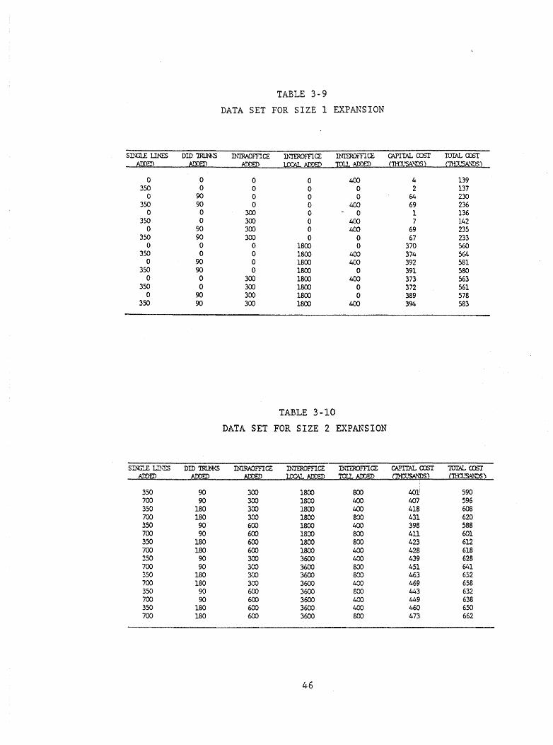
TABLE 3-9
DATA SET FOR SIZE 1 EXPANSION
srn:;u: UNES DID'lRlN!'S D\1RADITlCE ll.'TEROmCE INll.ROffiCE CAPITAL cnsr 1UIAl.. cnsr ADDED ADDED AOOED l1X'Al. AIDED :mu. ADDED (J1!2.'SA~) !1Hl~~}
0 0 0 0 400 4 139 350 0 0 0 0 2 137
0 90 0 0 0 64 230 350 90 0 0 400 69 236
0 0 300 0 0 1 136 350 0 300 0 400 7 142
0 90 300 0 400 69 235 350 90 300 0 0 67 233
0 0 0 1800 0 370 560 350 0 0 1800 400 374 564
0 90 0 1800 400 392 581 350 90 0 1800 0 391 580
0 0 300 1800 400 373 563 350 0 300 1800 0 372 561
0 90 300 1800 0 389 578 350 90 300 1800 400 394 583
TABLE 3-10
DATA SET FOR SIZE 2 EXPANSION
sm:;u: U!\ES DID '.IRJ.N<S INmAOrnCE mrEroma: Jl.."'I'ERDFFlc:e: CA.'Pl'IAL OJS! 'IOIAL CDS! .@Qm pmF!) /-J)'J--:D l.OCl\l.. ADD::D :m'~~ (~1$II.NDS) Crn::tlS.A...lOS '\
350 90 300 1800 800 401 i 590 700 90 300 1800 400 407 596 350 180 300 1800 400 418 608 700 180 300 1800 800 431 620 350 90 600 1800 "-00 398 588 700 90 600 lS::JO 800 411 601 350 180 600 1800 800 423 612 700 180 600 1800 400 428 618 350 90 300 3600 400 439 628 700 90 300 3600 800 451 641 350 180 300 3600 800 463 652 700 180 300 3600 400 469 658 350 90 600 3600 800 443 632 700 90 600 3600 400 449 638 350 180 600 3600 400 ~ 650 700 180 600 3600 800 473 662
46

TABLE 3-11
DATA SET FOR SIZE 3 EXPANSION
SIl'Q..E LINES OlD 1RlN~ D'ffit6Dma: nrroomCE mrOOFTIa: CAPITAL CDS! 'IUW. CDST ADDED @~ ADDED lOCAL ADDED 'ID~ ADDED nIDJSANDS} {n-n:rs.t>,.\"OS )
700 180 600 3600 1200 481 671 1050 180 600 3600 800 480 670
700 270 600 3600 800 653 8!.0 1050 270 600 3600 1200 658 845 700 180 900 3600 800 479 669
1050 180 900 3600 1200 4S4 674 700 270 900 3600 1200 657 844
1050 270 900 3600 800 656 843 700 180 600 ~ 800 670 856
1050 180 600 5400 1200 675 862 700 270 600 5400 1200 692 878
1050 270 600 5400 800 691 877 700 180 900 5400 1200 674 861
1050 180 900 5400 800 673 859 700 270 900 5400 800 690 875
1050 270 900 5400 1200 695 882
TABLE 3-12
DATA SET FOR SIZE 4 EXPANSION
sm;u: l..INES DID 1'Rl.N~ J:'.l\'"lRAOmCE Th"'I'ERDFFla:: nrrmomCE CAPITAL COS! TOTAL OJS'I ADOrn flm~ ADDm ~;.rom N..L fi1)J2:JJ ClJ-rxJSA~2 (1HJtJS~\1DS)
1050 270 900 5400 1600 702 889 1400 270 900 5400 l.2OO 700 887 1050 360 900 5400 l.2OO 808 995 1400 360 900 5400 1600 812 999 1050 270 1200 5400 1200 700 8S7 1400 270 1200 5400 1600 704 891 1050 360 1200 5400 1600 813 lCXXI 1400 360 1200 5400 1200 810 997 1050 270 900 7200 1200 9.!.4 1154 1400 270 900 7200 1600 948 1J.58 1050 360 900 7200 1600 1056 1266 1400 360 900 7200 1200 1054 1164 1050 270 1200 7200 1600 947 1157 1400 270 1200 7200 1200 945 1155 1050 360 1200 7200 1200 1053 1263 1400 360 1200 7200 1600 1057 1267
47
constraints force all adjacent size pieces of the spline model to agree at
their common boundary points.
An alternative to using the constrained least squares approach is to
fit the models independently and igtl0re any model disagreements at their
boundaries. In fact these disagreements were very small. In this approach
one would use the model for the smaller size expansions to evaluate a point
that is common to two adjacent sizes. Our preference is to add restriction
to the procedures that fit the models rather than add restrictions to how
the models may be used. -
The pilot data presented in tables 3-9 to 3-12 were analyzed using a
constrained least squares technique closely related to (but not the same as)
that defined for spline functions. The procedure was developed to use
existing software to approximate the spline function calculations. It has
subsequently been found that some versions of the SAS statistical analysis
system contain procedures that will allow direct computation of the spline
functions. When the direct calculation method has been applied to the pilot
data, the results differed from those presented here by insignificant
amounts.
The models derived from the pilot data using the constrained least
squares approach are given in tables 3-13 and 3-14. In these models the
following variable definitions are used:
Xl is the number of access lines added,
x 2 is the number of interswitch local busy-hour CCS added,
xs is the number of intraswitch busy-hour CCS added,
x 4 is the number of DID trunks added,
X5 is the number of interexchange busy-hour CCS added,
Yc is the capital cost (defined for income tax purposes) of an expansion, and
Yt is the total cost of an expansion.
The figures 3-2 through 3-9 were obtained by summing across the four pieces
of each model only those terms involving the variable being graphed. For
48
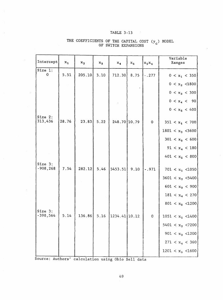
TABLE 3-13
THE COEFFICIENTS OF THE CAPITAL COST (y ) MODEL OF SWITCH EXPANSIONS c
Variable Intercept xl X 2 Xs X4 Xl) x 2 x 4 Ranges
Size 1: 0 5.51 205.10 3.10 712.30 8.75 -.277 0 < Xl < 350
0 < X2 <1800 -
0 < Xg < 300
0 < X 4 < 90
o < xl) < 400
Size 2: 313,436 28.76 23.83 5.22 248.70 10.79 0 351 < xl < 700
1801 < x 2 <3600
301 < Xs < 600
91 < x 4 < 180
401 < xl) < 800
Size 3: -908,268 7.54 282.12 5.46 5453.51 9.10 -.971 701 < Xl <1050
3601 < X2 <5400
601 < Xs < 900
181 < x 4 < 270
801 < xl) <1200
Size 3: -398,564 5.14 136.86 5.16 1234.41 10.12 0 1051 < xl <1400
5401 < x 2 <7200
901 < Xs <1200
271 < x4, < 360
1201 < xI) <1600
Source: Authors' calculation using Ohio Bell data
49
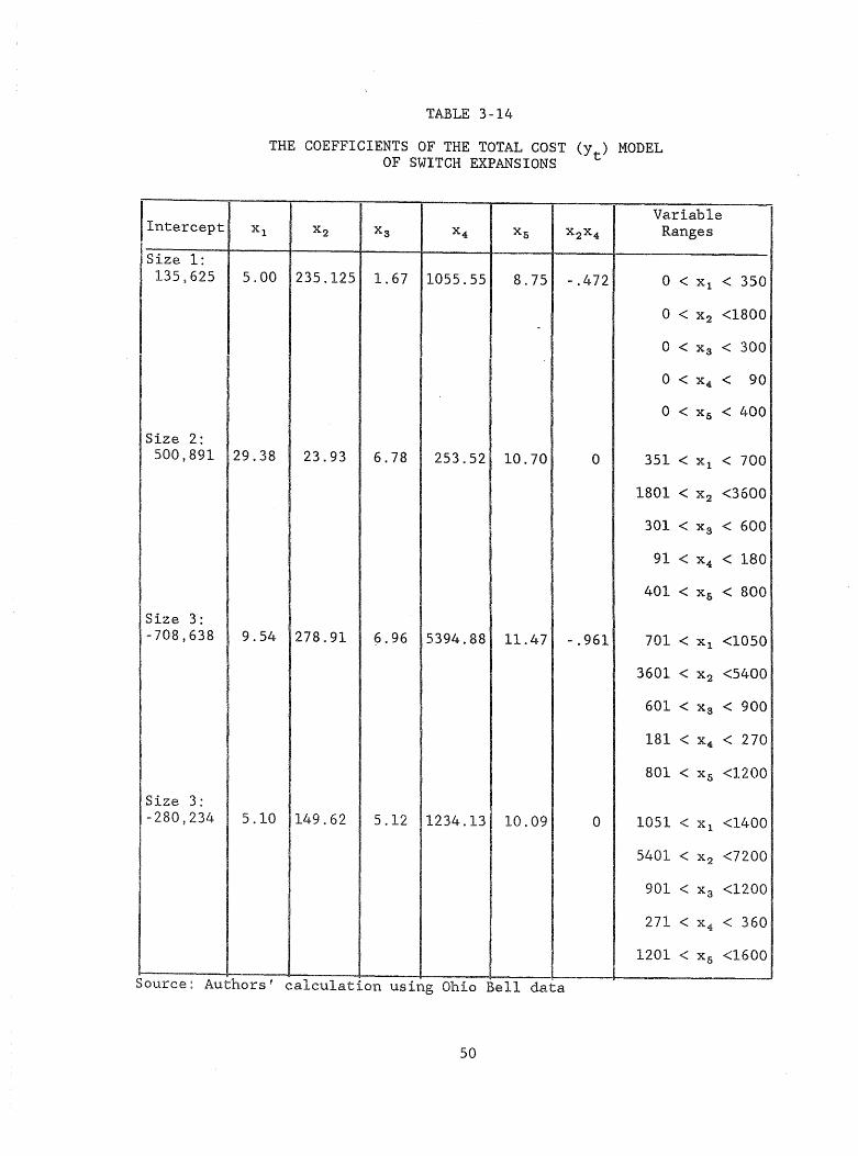
Intercept
Size 1: 135,625
Size 2: 500,891
Size 3: -708,638
Size 3: -280,234
TABLE 3-14
THE COEFFICIENTS OF THE TOTAL COST (Yt
) MODEL OF SWITCH EXPANSIONS
Variable Xl X2 Xs X4 Xs x 2x 4 Ranges
5.00 235.125 1.67 1055.55 8.75 -.472 o < Xl < 350
0 < X2 <1800 -
0 < Xs < 300
o < X" < 90
o < Xs < 400
29.38 23.93 6.78 253.52 10.70 0 351 < Xl < 700
1801 < x 2 <3600
301 < Xs < 600
91 < x 4 < 180
401 < Xs < 800
9.54 278.91 6.96 5394.88 11.47 -.961 701 < Xl <1050
3601 < X2 <5400
601 < Xg < 900
181 < x 4 < 270
801 < Xs <1200
5.10 149.62 5.12 1234.13 10.09 0 1051 < Xl <1400
5401 < x 2 <7200
901 < Xg <1200
271 < x 4 < 360
1201 < Xs <1600
Source: Authors' calculation using Ohio Bell data
50

Case
1
2
3
TABLE 3-15
THREE CASES FOR THE VALUE OF x 4
WHILE COMPUTING x 2 'S COST
Size
1 2- 1
0 90 180
90 90 180
90 90 270
Source: Authors' assumption
fl
270
270
270
example, consider access lines which was the variable of interest for figure
3-2. The contribution to cost of access lines is computed at $5.51 for each
of the first 350 lines, at $28.76 for each of the next 350 lines, at $7.54
for each line over 700 lines added but less than 1051 lines, and the
contribution of the last 350 lines added is computed at $5.14 each. A
similar calculation is made for the interswitch local busy-hour traffic, but
due to the cross product term, x2x4, in the size 1 and size 3 pieces of the
model, its contribution to cost is calculated under three cases given in
table 3-15.
Because the coefficient for the X 2 X 4 term is negative in the size 1 and
size 3 pieces of the models, a savings occurs when both DID trunks and
capacity for interswitch local busy-hour are added to the switch. The
calculations made for figures 3-4, 3-5, 3-8, and 3-9 B.llocated the entire
savings to the interswitch traffic variable. An alternate calculation could
have allocated the savings in some manner to both. An argument that favors
the former method is that a business customer adds DID trunks beca.use he
51

needs to pass more traffic through the system, including the interswitch
trunking. Thus, a cost savings resulting from a lower cost on the traffic
variable benefits the business customer when the total cost of all his
services is computed.
Some variables have an inconsistent effect on costs, both the capital
cost and the total cost. This is primarily due to the "lumpiness" of some
items of equipment as discussed earlier. One should also note that the
average cost curves tend to stabilize toward the right side of the graphs.
This is because as one moves to the right on the average cost curves,the
average is being taken over a larger and larger number of units. This has
the effect of smoothing out the lumpiness. When a sample of several
switches is used, an average over the switches should have the same effect.
Turn now to a process of averaging over the several switches in a sample,
and to the computation of a customer cost.
Step 6: Average
The computation of an average incremental cost 4 for a customer class
is relatively complicated. It requires the use of the CAPCOST model that
was developed as part of this project. The CAPCOST model is described in
Appendix D. The averaging technique also requires growth forecasts for each
switch in the sample. We shall explain the method by working through an
example in which we assume a hypothetical sample of three switches. One of
the three switches will be the one used in the pilot work but its growth
forecast is hypothetical. In the calculations that follow, any savings from
the joint addition of DID trunks and interswitch busy-hour traffic capacity
is all allocated to the interswitch busy-hour traffic capacity expansion.
One switch in the sample will be losing customers while the other two will
be gaining customers. For those switches gaining customers an initial step
is to "optimize" the expansion size. An average cost per unit for that size
4 Average incremental cost is the quantity that we estimate and then use as a proxy for marginal cost. In fact, increments of ca.pacity are added in a switch expansion rather than marginal units because the equipment is not infinitely divisible, thus a true marginal-cost calculation is not possible.
52
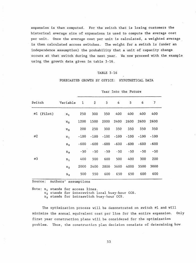
expansion is then computed. For the switch that is losing customers the
historical average size of expansions is used to compute the average cost
per unit. Once the average cost per unit is calculated, a weighted average.
is then calculated across switches. The weight for a switch is (under an
independence assumption) the probability that a unit of capacity change
occurs at that switch during the next year. We now proceed with the example
using the growth data given in table 3-16.
TABLE 3-16
FORECASTED GROWTH BY OFFICE: HYPOTHETICAL DATA
Year Into the Future
Variable 1 2 3 4 5
#1 (Pilot) xl 250 300 350 400 400
x 2 1200 1500 2000 2400 2600
xa 200 250 300 350 350
#2 Xl -100 -100 -100 -100 -100
x 2 -600 -600 -600 -600 -600
xa -50 -50 -50 -50 -50
#3 Xl 400 500 600 500 400
x 2 2000 2400 2800 3600 4000
xa 500 550 600 650 650
Source: Authors' assumptions
Note: Xl stands for access lines. x2 stands for interswitch local busy-hour ccs. Xg stands for intraswitch busy-hour CCS.
6
400
2600
350
-100
-600
-50
300
3500
600
7
400
2600
350
-100
-600
-50
200
3000
600
The optimization process will be demonstrated on switch #1 and will
minimize the annual equivalent cost per line for the entire expansion. Only
first year construction plans will be considered for the optimization
problem. Thus, the construction plan decision consists of determining how
53
many years of growth should be satisfied by the plant added in the first
year. The total cost of each construction plan can be determined from the
models given in table 3-14, or more easily by adding component costs read
from the curves given in figures 3-6 through 3-9. Figures 3-2 to 3-5 can be
used to obtain the corresponding capital cost, or the models in table 3-13
can be used for the same purpose. It should be noted that in figures 3-4
and 3-8 there are several curves to consider. We based the cost
contribution of interswitch traffic on two situations. In the first, we
assumed an annual demand for new DID trunks that was large enough to gain
the economies that are possible from the joint addition of trunks and
capacity for interswitch busy-hour traffic (i.e., we used the lower most
curve), In the second, we assumed no such economies because of insufficient
demand for DID trunks (i.e., we used the uppermost curve). The resulting
values can then be weighted with either their historical or their forecasted
probabilities of occurring, and added together to obtain a composite figure.
For this example, the weights we used were 0.5 and 0.5.
In this step the CAPCOST model is now run for each construction plan
using the capital cost as an input for the initial investment, and the
difference between the total cost and the capital cost as the entry for a
special expense in the first year. The fill rate will vary depending on
which plan is assumed, but it will be based on the number of lines added.
As a result, the one year plan uses a fill rate of 1 in each year, while the
two year plan will be filled to (250/550)ths of its capacity the first year
and will have a fill rate of 1 in all subsequent years. The three year plan
will have fill rates of 250/900 the first year, 550/900 the second year, and
1 each year thereafter. At the present time, operation and maintenance (0 &
M) costs have not been determined in this study so that they should be set
to zero for this step. It is unlikely that 0 & M costs will have an effect
on the optimal first year construction plan, although they will affect the
cost that must be recovered. Construction plans that go beyond four or five
years should not be considered because of the extreme uncertainty about
forecasts that far into the future. The CAPCOST solution is divided by the
number of lines added in the corresponding construction plan.
Table 3-17 gives the result of a CAPCOST run on the one year expansion
plan. The solution is divided by 250 to obtain an average annual per line
54

TABLE 3·17
CAPCOST MODEL OUTPUT
Capital Structure: Percentage composed of debt - 40.0% A'verage interest rate on debt - 9.0% Percent corrposed of equity - 60 . 0% Avg rate of retJ.u:n on equity - 16.0%
Composite Cost of Capital 13.2% Composite In:.ane Tax Rate - 46.0%
Solution: lower Bound: $65,614.04 Mid Point: $65,614.31 Upper Bound: $65,614.57
Width: $ 0.531426
FIll. SP£Cl.AL \'EAR ltAJt ~ EXPENSES
A :s c D
1 1 $65,614 $150,040 2 1 65.614 0 3 1 65,614 0 4 1 65,614 0 5 1 65.614 0 6 1 65,614 0 7 1 65.614 0 8 1 65,614 0 9 1 65,614 0
10 1 65,614 0 11 1 65,614 0 12 1 65,614 0 13 1 65,614 0 14 1 65,614 0 15 1 65,614 0
E NPV m: ($0.7634)
Req'd \.,lidth: $1.000000
O&M BXJK CDS'l'S DE:P
E r
$0 $25,716 0 25,716 0 25,716 0 25,716 0 25,716 0 25,716 0 25,il6 0 25,716 0 25,716 0 25,716 0 0 0 0 0 0 0 0 0 0
55
Other Infonnation: Horizon - 15 Initial .a.rtOLIl1t i.nvested - $257,160 Regulatory book life 10 Tax life 5 Tax depreciation method - ACPS OSM grO\o,'th rate 0.0% 05M gradient change $0.00 OSM ini tia! cost $0.00 Gorrpertz -Makeham pararreters:
s - 0 g - 0 c - 0
NX !CQ{ TAX D~ AtX TAX DEl' DEP W:ES ~ ).'FAR
G Ii I J K
$ 25,716 $51,432 $11,829 $11,829 1 51,432 82,291 26,025 37,854 2 77,148 61,718 16,561 54,415 :3
102,864 41,146 7,098 61,513 4 128,580 20,573 ( 2,366) 59,147 5 154,296 0 ( 11,829) 47,317 6 180,012 0 ( 11,829) 35,488 7 205,728 0 ( 11,829) 23,659 a 231,444 0 ( 11,829) 11,829 9 257,160 0 ( 11,829) 0 10 257,160 0 0 0 11 257,160 0 0 0 12 257,160 0 0 0 13 237.160 0 0 0 14 257,160 0 0 0 15
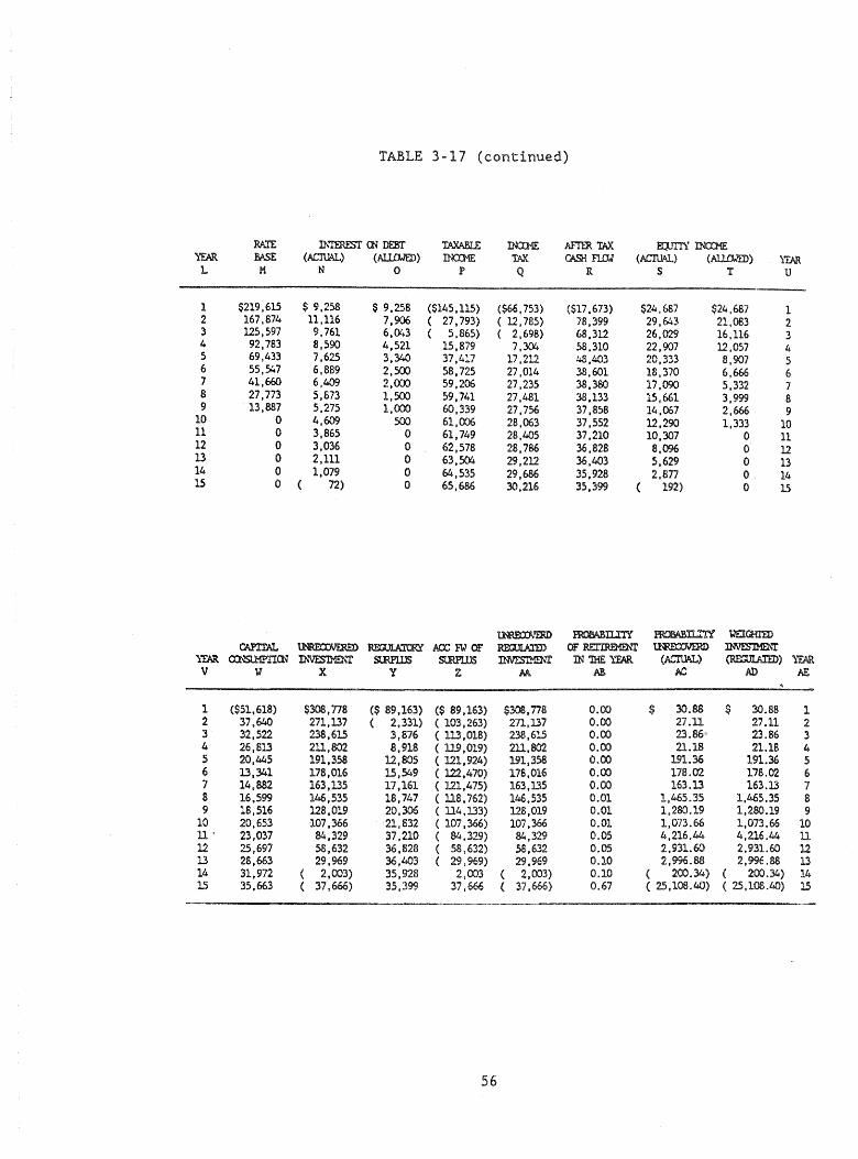
TABLE 3-17 (continued)
RATE ll\"TEREST rn DE8I' TAXABl.E llm'IE AFTI.'R TAX F.QJITY IN:X'ME i'fAR BASE (ACTllAL) (Al.l.DJfD ) IN:Jl1E !AX CASH F'11J.J (ACIUAL) (AJJ..D...'ED ) \'EAR L M N 0 r Q R S T U
1 $219,615 $ 9,2SS $ 9,258 ($145,115) ($66,753) ($17,673) $24,687 $24,687 1 2 167,874 11,116 7,906 ( 27,793) ( 12,785) 78,399 29.643 21,083 2 3 ill ,597 9,761 6,043 ( 5,865) ( 2,698) 68,312 26,029 16,116 :3 4 92.783 8,590 4,521 15.879 7,304 58,310 22.907 12,057 4 5 69,433 7.625 3,340 37,417 '"'I '1' ') J.O J.I'\':I 20.333 o ""., 5 ..&.1,4....L.4 ...-u,""'V.J 0, :lV1 6 55,547 6,889 2,500 58,725 27,014 38,601 18,370 6,666 6 7 41,660 6,409 2,000 59,206 27,235 38,380 17,090 5,332 7 8 27,773 5,873 1,500 59,741 27,481 38,133 15,661 3,999 8 9 13,887 5,275 1,000 60,339 27,756 37,SSS 14,067 2,666 9
10 0 4,609 500 61,006 28,063 37,552 12,290 1,333 10 11 0 3,865 0 61.749 28,405 37,210 10,307 0 11 12 0 3,036 0 62.578 28,786 36,828 8,096 0 12 13 0 2,111 0 63,504 29,212 36,403 5,629 0 13 14 0 1,079 0 64.535 29,686 35,928 2,877 0 14 15 0 72) 0 65.686 30,216 35,399 192) 0 15
'I.N'{£O'j\'mD PRCfJABII...!1Y PRClBASD....."'"'!Y WEIGmD CAPl'rAL ~ Rm.ll.A.l'C:RY MX FW or :Rm.l1.Al1D or RErDIDID,'r ~ ~"l'
i'EAR cmst.MPl1c:N ll\~"I' SLRPl.lJS SUiU'llJS ~'T IN '!HE l.'EAR (A.."'.nW..) (RmJl.Al"fD) i'EAR. V \3 X Y Z M M- AC MJ M..
1 ($51.618) $308,778 ($ 89,163) ($ 89,163) $308.778 0.00 $ 30.88 $ 30.88 1 2 37,640 271,137 ( 2,331) ( 103,263) 271,1.37 0.00 27.11 27.11 :2 :3 32.522 238.615 3,676 ( m,OIS) 238,6!.5 0.00 23.86 23.86 3 4 26,813 211,802 8,918 ( 119,019) 2U,802 0.00 21.18 21.18 4 5 20,445 191,358 12,805 ( 121,924) 191,358 0.00 191.36 191.36 5 6 13,341 178,016 15,549 ( 122,470) 176,016 0.00 178.02 178.02 (,
7 14,882 163,135 17,161 ( 121,475) 163.135 0.00 163.13 163.13 7 S 16,599 146,535 18,747 ( 118,762) 146,535 0.01 1,465.35 1,465.35 8 9 18,516 128,019 20,306 ( 114,133) 128,019 0.01 1,280.19 1,280.19 9
10 20,653 107,366 21,832 ( 107,366) 107,366 0.01 1,073.66 1,073.66 10 U' 23,037 84,329 37,210 ( 84,329) 84,329 0.05 4,216.44 4,216.44 II 12 25,697 58,632 36,828 ( 58,632) 58,632 O.OS 2.931.60 2,931.60 12 13 28,663 29,969 36,403 ( 29,969) 29,969 0.10 2.996.88 2,9%.88 13 14 31,972 2,00:3) 35,928 2,003 2,003) 0.10 ( 200.34) ( 200.34) 14 15 35,663 37,666) 35,399 37,666 37,666) 0.67 ( 25,108.40) ( 25,108.40) 15
56
cost of $262. Similar results for the two year, three year and four year
plans give average annual per line costs of $178, $142, and $176,
respectively. From these figures we see that the plan producing the lowest
annual cost per line is the three year plan.
Once the optimal size expansion is determined, the CAPCOST model is run
for each of the three components of cost corresponding to access lines,
intraswitch busy-hour traffic, and interswitch busy-hour local traffic.
Thus, a per-unit annual cost is determined for each variable.
Switch #2, which is losing customers, is treated differently than the
others. Here we use a company-wide historical average size expansion as a
standard and use the CAPCOST model to solve for the annual cost of this
average expansion but with a declining fill rate. For example, suppose the
average number of lines added during past switch expansions has been 400.
We determine the capital cost and total cost of such expansions from either
the models or figures 3-2 and 3-6 as before. These are entered in th~
CAPCOST model as usual. The fill rate, however, is set to 1 in the first
year, and using the data in table 3-16 where 100 lines are lost annually,
the fill rate is 300/400 in the second year, 200/400 the third year, 160/400
the fourth year, and 0 the fifth and all successive years. The CAPCOST
solution is divided by 400 lines to get the average cost per line. This
figure represents the cost per line of having those 400 lines available
while they are being placed out of service. The fact that 400 lines was
used as the base is perhaps of little significance, but using historical
data to determine the base number will certainly pass a reasonableness test.
In the sample calculations, it was assumed that no equipment is
salvaged as customers leave the switch. This assumption was made to
simplify the example but should not be carried over to a study of actual
switches that are losing customers. The reason is that much of the
expensive electronic equipment in these switches consists of plug-in modules
that can be removed from one switch and plugged into another. The computer
aided design system used by Ohio Bell to configure their 1 and lA ESS
switches can provide estimates of the value of salvaged equipment. Such
information could be used to adjust the cost of the switches that are losing
customers. One may need also to consider the average vintage of the most
recent additions to switches that now have negative growth, rather than
assume (as we have done here) that the expansion occurs and is fully filled
57

immediately before customers begin leaving the switch. Given the
appropriate data, the requisite adjustments to the analysis can be
accomplished with the CAPCOST model.
In the case of switch #2, the result for access lines was $5.05; for
the intraswitch busy-hour CCS, $1.48 was the solution with an assumed
average expansion size of 400 CCS; and the interswitch busy-hour CCS figure
was $126.46 with an average expansion size of 2000 CCS. All the average
expansion sizes are hypothetical values for illustrative purposes only,
since the required historical data have not been scientifically gathered as
part of the pilot study. These values are plausible, however.
Table 3-18 summarizes the values obtained from the CAPCOST analyses
described above for switches #1 and #2, and it gives hypothetical, but
plausible, corresponding values for switch #3.
The final step is to average the cost of each variable across the three
switches. This average is a weighted average where the weight for a switch
is the proportional amount of the first year's activity in all switches that
takes place in the particular switch. An activity is defined to be either a
reduction or an increase in the number of units of the variable. If the
activities that take place are all independent events, then these weights
TABLE 3-18
THE AVERAGE, ANNUAL, PER-UNIT COST FOR THREE VARIABLES IN THREE SWITCHES
Variable Switch
Symbol Description #1 #2 #3
Access lines $ 3.24 $ 5.05 $ 1.55
Interswitch local busy-hour ees 22.18 126.46 23.90
Intraswitch busy-hour ees 1.10 1.48 0.82
Source: Authors' calculations with pilot cost data in switches and #2, and authors' assumed growth data for all switches and assumed model coefficients for switch #3
58
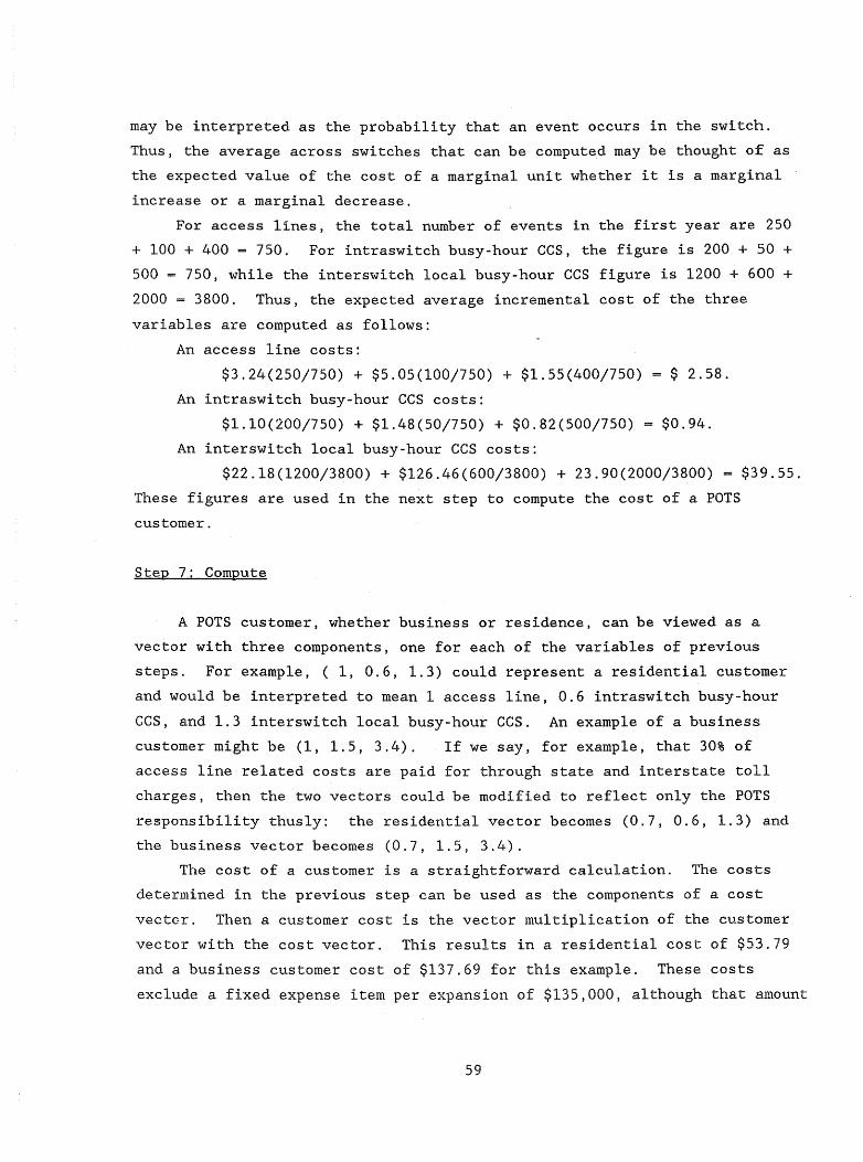
may be interpreted as the probability that an event occurs in the switch.
Thus, the average across switches that can be computed may be thought of as
the expected value of the cost of a marginal unit whether it is a marginal
increase or a marginal decrease.
For access lines, the total number of events in the first year are 250
+ 100 + 400 = 750. For intraswitch busy-hour CCS, the figure is 200 + 50 +
500 = 750, while the interswitch local busy-hour CCS figure is 1200 + 600 +
2000 = 3800. Thus, the expected average incremental cost of the three
variables are computed as follows:
An access line costs:
$3.24(250/750) + $5.05(100/750) + $1.55(400/750)
An intraswitch busy-hour CCS costs:
$1.10(200/750) + $1.48(50/750) + $0.82(500/750)
An interswitch local busy-hour CCS costs:
$ 2.58.
$0.94.
$22.18(1200/3800) + $126.46(600/3800) + 23.90(2000/3800) = $39.55.
These figures are used in the next step to compute the cost of a POTS
customer.
Step 7: Compute
A POTS customer, whether business or residence, can be viewed as a
vector with three components, one for each of the variables of previous
steps. For example, ( 1, 0.6, 1.3) could represent a residential customer
and would be interpreted to mean 1 access line, 0.6 intraswitch busy-hour
CCS, and 1.3 interswitch local busy-hour CCS. An example of a business
customer might be (1, 1.5, 3.4). If we say, for example, that 30% of
access line related costs are paid for through state and interstate toll
charges, then the two vectors could be modified to reflect only the POTS
responsibility thusly: the residential vector becomes (0.7, 0.6, 1.3) and
the business vector becomes (0.7, 1.5, 3.4).
The cost of a customer is a straightforward calculation. The costs
determined in the previous step can be used as the components of a cost
vector. Then a customer cost is the vector multiplication of the customer
vector with the cost vector. This results in a residential cost of $53.79
and a business customer cost of $137.69 for this example. These costs
exclude a fixed expense item per expansion of $135,000, although that amount
59

was included in the optimization step. Since it is a fixed expense, it does
not vary with the amount of capacity for lines or traffic added in an
expansion. For the optimal size expansion, this fixed expense item
annualizes to $23.13 per line. Allor a portion of this cost may be spread
to the two POTS customer classes on the basis of lines or some other
reasonable factor. For purposes of example, suppose that 70% is to be
spread on the basis of lines, and that in the sample switches three quarters
of all lines added are expected to go to residential POTS customers while
one quarter will go to business POTS customers. This increases the cost for
residential customers to $65.93 per year or $5.49 per month. The cost for
business customers increases to $141.73 per year or $11.81 per month.
Summary and Findings
A method has been presented that computes, as a final result, the
marginal cost of a marginal customer whose service is provided by adding
capacity to an existing switch. The method is also applicable, with some
modification, to estimating costs for customers whose service is provided by
a totally new facility. Such modified estimates would need to include the
cost of the central processing unit (CPU) and related equipment. The
expansion costs computed in this chapter do not include any CPU costs. The
particular problem with the CPU cost is that it is a very lumpy piece of
equipment whose cost is probably unrelated to the variables we have used to
describe the customer vector. Lumpiness can be handled by averaging over
incremental additions of plant, but being unrelated to the variables that
describe customers is a fixed-cost problem. Fixed costs will have to be
allocated. This study has not addressed the problem of allocating fixed
costs other than those arising as part of a switch expansion. Some of the
ideas expressed could apply to fixed costs resulting from the installation
of a new CPU.
The critical question with respect to our method is whether it is
possible to apply it to derive at least part of the marginal cost of a
customer. Certainly the computations prescribed in the method are possible
if the data needed for the calculations can be obtained. Since the method
works with a sample of switches, the question of data availability pertains
to each switch in the sample. Since the pilot study involved developing the
60
requisite data for an actual switch, it serves to demonstrate that, indeed,
such data can be acquired to perform the specified calculations. The only
assumed data for the pilot switch was the forecasted growth in service
requirements. Such forecasts are routinely made in the Ohio Bell system and
are certainly necessary for every telephone company in order to make
informed capacity decisions. Thus, the forecasted data should be readily
available and could be provided independently by the PUCO, given available
historical data on customer use of telephone services.
A second favorable disclosure of the pilot study was the result that
the cost structure for the variables that describe a customer was a very
simple structure, making it easy to use. Moreover, it was almost completely
separable from the costs for interexchange traffic. The only non"separable
part was the fixed expense associated with an expansion but which was also
unrelated to the nature of the expansion. While we did suggest methods for
allocating the fixed costs, our basic view is that a cost study should
generally not allocate costs but should estimate and identify the various
components of cost including fixed costs and variable costs. The problem of
how all the costs should be recovered is a pricing matter, the solution to
which must be based on cost information as well as the objectives being
sought by a pricing policy.
61


CHAPTER 4
CONCLUSIONS AND RECOMMENDATIONS
In the first chapter a number of questions were raised. Included among
these was what are the appropriate costs and what methods can be used to
compute a cost figure for each part of the local network? The first step in
developing methods to compute the costs of the different parts of POTS
service is to develop a method for one part. This was done for one of the
major parts of the system, COE. Procedures have been included to provide
some optimization of costs vis-a-vis forecasted service requirements and to
annualize these costs. Both of these steps (optimization and annualization)
bring the results of the method close to what has been demonstrated to be,
on theoretical grounds, the appropriate cost.
What has not been fully addressed as yet is the usefulness of the
marginal cost values to solve actual pricing problems. While the long-run
marginal cost or its practical equivalent, the average incremental cost, was
discussed in chapter 2 where it was concluded that such costs are
theoretically the most useful in setting prices, the question remains as to
how such costs can be used as a practical matter. Perhaps the best way to
answer that is with an example. We quote from a recent monograph by Park
and Mitchell who were reporting on an assessment of peak-load pricing for
telephone calls: 1
Capacity costs will vary with the number of calls (or minutes) that the telephone switching equipment and trunk lines are designed to serve. We are interested1 in the additional cost of serving one additional call per hour and use the annual equivalent of the incremental investment cost, reflecting such factors as yearly interest, depreciation, maintenance, and taxes.
Because the equipment is available only in IIlumps ,1I
the cost must actually be estimated as the average incremental cost over some wider range of alternative capacities.
1 Park, Rolla E" and Mitchell, Bridger, M., Optimal Peak-Load Pricing for Local Telephone Calls, The Rand Corporation, Santa Monica, CA (1986), p. 14.
63

Park and Mitchell could not have performed their analysis of a peak
load pricing policy without the cost figure described by them in the above
excerpt. We point out that the type of cost figure that they have described
is exactly the type that the method in this report will determine. The
actual number that they used came from a 1980 Mountain Bell filing for
measured rates in Arizona. In addition, their analysis required usage data
and price elasticities which they obtained from the 1976 Illinois
experiments conducted by GTE.2 Park and Mitchell concluded that feasible
peak-load pricing schedules would at best result in only modest efficiency
gains, and would more likely result in small efficiency losses.
The key point is that if economic efficiency is at least one of the
pricing goals, then it is of fundamental importance to acquire the type of
cost data obtainable by the method in our report as well as data about usage
patterns of the various customer classes and their price elasticities. If
there is no goal of economic efficiency, but instead the goal is to simply
cover the booked costs, then approximate long-run marginal costs are not
needed.
Our recommendation is that the method described in chapter 3 be
undertaken with a sample of from 10 to 15 offices in the Ohio Bell
territory, and that-simultaneously with that effort procedures be found to
incorporate 0 & M expenses and the investment cost of the CPU. We reiterate
the recommendation that the 8 point experimental plan be used on these
sample offices so that a better understanding can be gained of the cost
savings that occur when DID trunks and interoffice traffic capacity are
added in the same expansion. The average costs obtained from such a study
can be directly applied in the next rate case when combined with usage data
and loop costs presently being gathered by Ohio Bell.
2 Cohen, G., "Measured Rates Versus Flat Rates: A Pricing Experiment," presented at the Fifth Annual Telecommunciations Policy Research Conference, Airlie, VA, March 1977.
64

APPENDIX A
TECHNICAL DISCUSSION
Problem Analysis
This study is a continuation of research begun by Constas. 1 Constas
expressed the cost of expanding an existing office as a function of the
growth of single lines, DID trunks, intraoffice usage and interoffice local
usage. In his model Constas assumed that the total interoffice toll usage
in a central office is constant, but recommended that this factor be
examined in a future study. The research described in this report follows
up on Constas' earlier work and incorporates interoffice toll usage into a
model that estimates the capital cost of a capacity expansion in a IA ESS
central office. This appendix presents a detailed description of the
experimental design as well as the technical terms and procedures.
Factorial Design
There are five variables that affect the cost of a capacity expansion
in a central office.
(1) Growth of single lines (2) Gro~th of direct in dial (DID) business trunks (3) Growth of intraoffice usage (4) Growth of interoffice local usage (5) Growth of interoffice toll usage
The traffic measures, items 3, 4 and 5, are in (CCS) hundred call
seconds units. The same four sizes, found in the Constas thesis, are used
here. There are no structural differences among the four sizes. These four
1 Constas, Anthonios (1985). Incremental Capital Costs of Local Telephone Service. Masters' thesis, unpublished. Columbus, Ohio: The Ohio State University.
65
sizes differ only in the size of the various expansion scenarios used to
obtain the data for estimating the parameters of the model.
Design of Experiment
1. Factorial design: Factorial designs are widely used in
experiments involving several factors where it is necessary to study both
the individual and joint effects of these factors on a response. A
particular case might involve k factors; each at two levels, "high" and
"low." These levels may be quantitative or qualitative. A complete
replicate of such a design requires 2*2* ... *2 = 2k observations, and is
called a 2k factorial design.
The main effect of a factor may be defined as the change in response
produced by the change in the level of the factor. A factor is usually
denoted by a capital letter. The high level of a factor in a treatment
combination is denoted by- the presence of the respective lower case letter,
while the low level is denoted by the absence of the corresponding letter.
As an example, suppose that three factors, A, B, and C, each at two 3
levels, are under study. The design is called a 2 factorial, and eight
treatment combinations are displayed in standard order as (1), a, b, ab, c,
ac, bc, and abc. An observation taken under the high level of A and C and 3
the low level of B is represented by ac. The observations of a 2 factorial
design that involve quantitative factors may be equivalently described by
the following linear regression model:
where fio is the overall average effect, fil' fi2 and fis are the main effects,
and fi4' fisl fi6 and fi1 are interaction effects.
As the number of factors increase in an experiment, the number of runs
required for a complete replicate of the design rapidly outgrows the
resources of most experimenters. In this research there are five factors.
66
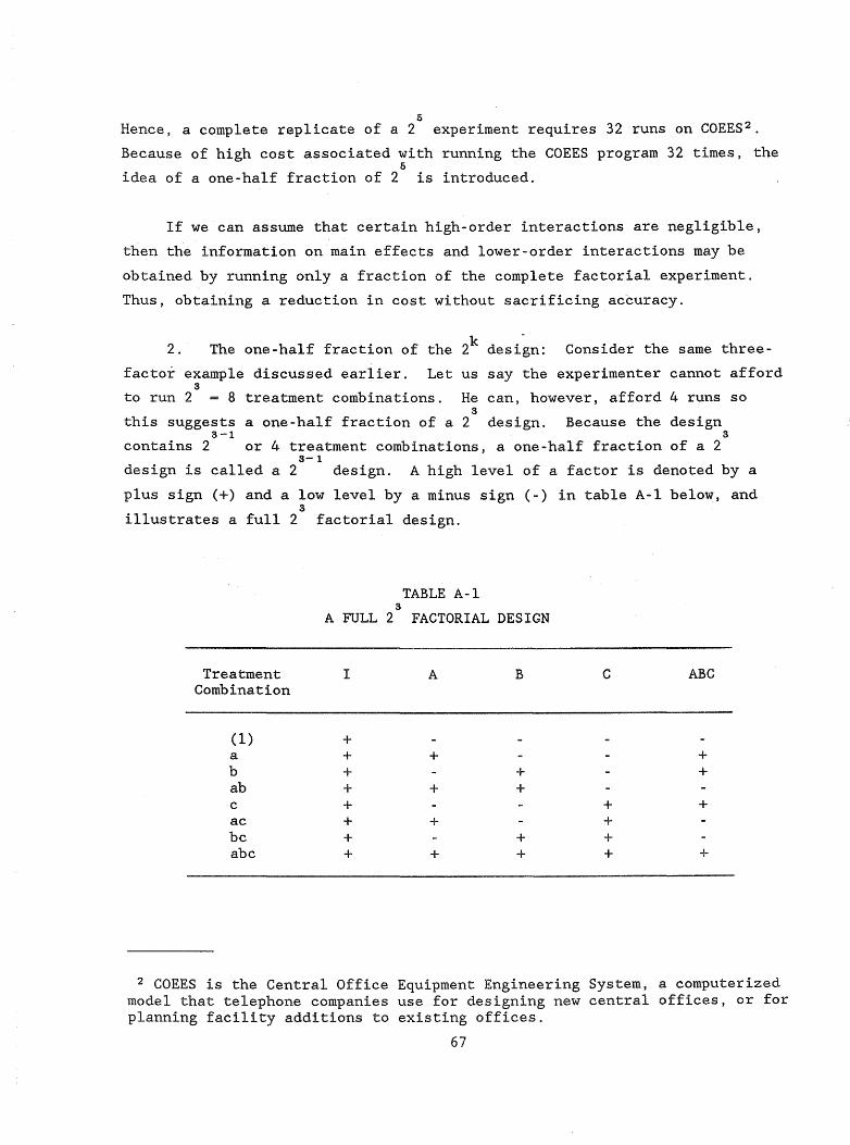
5 Hence, a complete replicate of a 2 experiment requires 32 runs on COEES2.
Because of high cost associated with running the COEES program 32 times, the 5
idea of a one-half fraction of 2 is introduced.
If we can assume that certain high-order interactions are negligible,
then the information on main effects and lower-order interactions may be
obtained by running only a fraction of the complete factorial experiment.
Thus, obtaining a reduction in cost without sacrificing accuracy.
2.· The one-half fraction of the 2k design: Consider the same three
factor example discussed earlier. Let us say the experimenter cannot afford 3
to run 2 = 8 treatment combinations. He can, however, afford 4 runs so 3
this suggests a one-half fraction of a 2 design. Because the design 3-1
contains 2 3
or 4 treatment combinations, a one-half fraction of a 2 3-1
design is called a 2 design. A high level of a factor is denoted by a
plus sign (+) and a low level by a minus sign (-) in table A-I below, and 3
illustrates a full 2 factorial design.
TABLE A-I 3
A FULL 2 FACTORIAL DESIGN
Treatment I A B C ABC Combination
(1) + a + + + b + + + ab + + + c + + + ac + + + bc + + + abc + + + + +
2 COEES is the Central Office Equipment Engineering System, a computerized model that telephone companies use for designing new central offices, or for planning facility additions to existing offices.
67

3-1 The 2 design is formed by selecting only those treatment
combinations that yield a plus sign on the ABC effect. The ABC term is
called the generator of this particular fraction. Furthermore, the identity
element I is always plus, so I = ABC is called the defining relation for the
design. S-l
To avoid making 32 runs on the COEES, a 2 design may be used. This
implies that the number of runs has decreased from 32 to 16. To decide
which 16 out of the 32 treatment combinations to select, the following
defining relation for the design is chosen:
where
I ABCDE
A Single lines added B DID trunks added C Intraoffice usage added D Interoffice local usage added E Interoffice toll usage added
The selection criterion is based on selecting the 16 scenarios
(treatment combinations) that yield a plus sign on the ABCDE effect (see
tables A-2, A-3).
68

TABLE A-2
FULL FACTORIAL DESIGN
Treatment I A B C D E ABCDE Combination
(1) + a + + + b + + + ab + + + e + + + ae + + + be + + + abc + + + + + d + + + ad + + + bd + + + abd + + + + + cd + + + aed + + + + + bed + + + + + abed + + + + + e + + + ae + + + be + + + abe + + + + + ee + + + ace + + + + + bee + + + + + abee + + + + + de + + + ade + + + + + bde + + + + + abde + + + + + ede + + + + + aede + + + + + bede + + + + + abede + + + + + + +
69
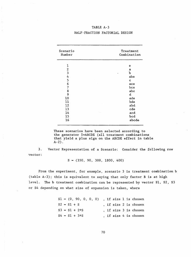
TABLE A-3
HALF-FRACTION FACTORIAL DESIGN
Scenario Treatment Number Combination
1 e 2 a 3 b 4 abe ~ c ;;)
6 ace 7 bce 8 abc 9 d
10 ade 11 bde 12 abd 13 cde 14 acd 15 bcd 16 abcde
These scenarios have been selected according to the generator I=ABCDE (all treatment combinations that yield a plus sign on the ABCDE effect in table A-2) .
3. Vector Representation of a Scenario: Consider the following row
vector:
S (350, 90, 300, 1800, 400)
From the experiment, for example, scenario 3 is treatment combination b
(table A-3); this is equivalent to saying that only factor B is at high
level. The b treatment combination can be represented by vector Sl, S2, S3
or S4 depending on what size of expansion is taken, where
Sl (0, 90, 0, 0, 0) if size 1 is chosen
S2 Sl + S if size 2 is chosen
S3 Sl + 2*S if size 3 is chosen
S4 Sl + 3*S if size 4 is chosen
70
Similar analyses were done to find the vector representation of all 15
remaining scenarios in the four different sizes. It shall be noted here
that one run of COEES will produce a solution for a scenario in all four
size expansions.
Regression Analysis
Data Request
A data request was sent to Ohio Bell in November of 1985 (exhibit 1,
found at the end of this appendix). This request contained the sixteen
scenarios (treatment combinations) that the one-half fraction design
selected. Each scenario was made up of eight alternatives. These
alternatives depended on the size of expansion that might be decided in a
specific year. In addition, each alternative had up to four possible jobs.
A job is an actual task of adding capacity in a given year. Since the study
was to examine the cost of an expansion made now, rather than an expansion
made a year or more from now, only the first job (job 1) was considered.
The output of each of the 16 runs contained an equipment list for every
alternative and its corresponding costs (capital, expense, removal, grand
total). An equipment list itemized the amount and type of equipment present
before the expansion, and the number and type added or "removed to satisfy a
given scenario.
Because of the balance in the experiment achieved with factorial
designs, the data are arranged in a special form. This form helps in
searching for patterns in the data that are useful in error checking and for
explaining discrete jumps in capital costs due to lumpiness. Four tables
are formed since four sizes of expansion are possible (tables 3-1, 3-2, 3-3
and 3-4 in chapter 3). To construct each table, all 16 scenarios are listed
as column headings and an exhaustive list of all equipment as row headings.
The data from the 16 output runs for the four tables are summarized in table
A-4.
71
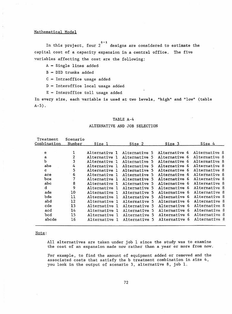
Mathematical Model
5-1 In this project, four 2 designs are considered to estimate the
capital cost of a capacity expansion in a central office. The five
variables affecting the cost are the following:
A Single lines added
B DID trunks added
C Intraoffice usage added
D Interoffice local usage added
E Interoffice toll usage added
In every size, each variable is used at two levels, "high" and "low" (table
A-5) .
Treatment Combination
e a b abe c ace bce abc d ade bde abd cde acd bcd abcde
Note:
Scenario Number
I 2 3 4 5 6 7 8 9
10 11 12 13 14 15 16
TABLE A-4
ALTERNATIVE AND JOB SELECTION
Size I Size 2
Alternative I Alternative 5 Alternative I Alternative 5 Alternative 1 Alternative 5 Alternative 1 Alternative 5 Alternative 1 Alternative 5 Alternative I Alternative 5 Alternative 1 Alternative 5 Alternative 1 Alternative 5 Alternative 1 Alternative 5 Alternative 1 Alternative 5 Alternative 1 Alternative 5 Alternative 1 Alternative 5 Alternative 1 Alternative 5 Alternative 1 Alternative 5 Alternative 1 Alternative 5 Alternative 1 Alternative 5
Size 3 Size 4
Alternative 6 Alternative Alternative 6 Alternative Alternative 6 Alternative Alternative 6 Alternative Alternative 6 Alternative Alternative 6 Alternative Alternative 6 Alternative Alternative 6 Alternative Alternative 6 Alternative Alternative 6 Alternative Alternative 6 Alternative Alternative 6 Alternative Alternative 6 Alternative Alternative 6 Alternative Alternative 6 Alternative Alternative 6 Alternative
All alternatives are taken under job 1 since the study was to examine the cost of an expansion made now rather than a year or more from now.
For example, to find the amount of equipment added or removed and the associated costs that satisfy the b treatment combination in size 4, you look in the output of scenario 3, alternative 8, job 1.
72
8 8 8 8 8 8 8 8 8 8 8 8 8 8 8 8
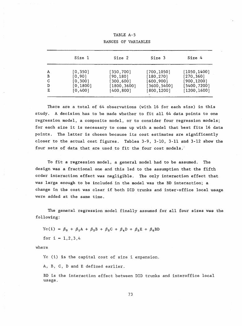
Size 1
A [0,350] B [0,90] C [0,300] D [0,1800] E [0,400)
There are a total of
study. A decision has to
TABLE A-5
RANGES OF VARIABLES
Size 2 Size 3 Size 4
[350,700] [700,1050] [1050,1400] [90,180] [180,270] [270,360] [300,600] [600,900] [900,1200] [1800,3600] [3600,5400] [5400,7200] [400,800] [800,1200] [1200,1600]
64 observations (with 16 for each size) in this
be made whether to fit all 64 data points to one
regression model, a composite model, or to consider four regression models;
for each size it is necessary to come up with a model that best fits 16 data
points. The latter is chosen because its cost estimates are significantly
closer to the actual cost figures. Tables 3-9, 3-10, 3-11 and 3-12 show the
four sets of data that are used to fit the four cost models.
To fit a regression model, a general model had to be assumed. The
design was a fractional one and this led to the assumption that the fifth
order interaction effect was negligible. The only interaction effect th.at
was large enough to be included in the model was the BD interaction; a
change in the cost was clear if both DID trunks and inter-office local usage
were added at the same time.
The general regression model finally assumed for all four sizes was the
following:
Yc(i)
for i 1,2,3,4
where
Yc (i) is the capital cost of size i expansion.
A, B, C, D and E defined earlier.
BD is the interaction effect between DID trunks and interoffice local usage.
73

EXHIBIT 1 OF APPENDIX A
25 FRACTIONAL FACTORIAL EXPERIMENTAL CONSTRUCTION PLAN PROJECT NAME: MARGINAL COST OF PLAIN OLD TELEPHONE SERVICE (POTS)
by
Clark A. Mount-Campbell Associate Professor of Industrial and
Systems Engineering
Baumin Lee Graduate Research Associate
THE NATIONAL REGULATORY RESEARCH INSTITUTE Columbus, Ohio
November, 1985
74
SCENARIO 1
TABLE 1A
Busy Season 1 - 2 3 4
Variables
Grow:th of single lines 350 350 350 350
Growth of DID trunk 0 90 90 90
. , Growth of intraoffice busy hour usage (CCS) 0 300 300 300
Growth of interoffice busy hour local usage
(CCS) 0 1800 1800 1800
Growth of inter exchange busy hour traffic (CCS )' 0 400 400 400
75
SCENARIO 1 TABlE 1B * Alternative 1 * Alternative 2 * Alternative 3 * Alternative 4 *
*------------------------*---------------*--------------*~-------------*--------------~* Busy Season 1: 2 3 : 4 : 1 : 2 3 : 4 : 1 2 3:4 1 2 3:4
Variables
: GrCMth of single lines 350: 350' 350: 350' 350: 350: 700' 350:1050' 350: 700: - 350:
: GrCMth of DID trunk 0' 90: 90: 90: 0: 90: 180: - 0' 270: - 0' 180: - 90:
: GrONth of intraoffice . , , , , ,
0: 600' - 300' ! : bus.Y hour usage (0:$) 0: 300: 300: 300: 0' 300' 600' 0: 900' -
: GrCMth of interoffice : buS'\' hem" local uSage ( 0:$) • 0:1800:1800:1800: 0'1800'3600: 0:5400: - 0:3600: - :1800'
: Growth of interexchange , , , busy hem" traffic (0:$) 0: 400: 400: 400: 0' 400: 800' - 0'1200: - 0' 800: - 400' , ! !
TABLE 1B conti.rued * Alternative 5 * Alternative 6 * Altemative 'J * Alternative 8 * * * * * * *
Busy Season : 1 : 2 : 3 : 4 : 1 : 2 : 3 : 4 : 1 2 : 3 : 4 : 1 : 2 : 3 : 4
Variables : : : : : : : : :
Growth of single lines : 700' 700; :1050' - 350' 700; - 350' 350'1400' -: : : :
GrcJv;rth of DID t:runk 90' lSO' lSO' 90' 99: - 90' 90' 270: -, ,
: Growth of intraoffice , b'.lsV hour usage (o:s) 300: 600' 600' 300' 300: - 300'300: 900: -! ,
: Growth of interoffice : , busy hour local usage (0:$) :1800: :3600: :3600: :1800:1800: - : 1800: 1800: 5400: -: Growth of interexcha:nge , busv hour traffic (0:$) : 400: BOO' BOO: : 400: 400' . : 400:400 :1200 -,
76
SCENARIO 2
TABLE 2A
Busy Season 1 2 3 4
Variables
: Growth of single lines 0 350 350 350
Growth of DID trunk 90 90 90 90
Growth of intraoffice busy hour usage (CCS) 0 300 300 300
Growth of interoffice busy hour local usage
(CCS) 0 1800 1800 1800
Growth of interexchange busy hour traffic (CCS) 0 400 400 400
77
*
SCENARIO 2 TABLE2B
Busy
* Alternative 1 * Alternative 2 * Alternative 3 * Alternative 4 * * * * * *
Season 1 2 3 : 4 123 412 3 : 4 : 1 2 3 : 4 Variables
; Growth of single lines 0: 350'350 : 350: 0: 350: 700: 0:1050: 0' . 350: 350:
: GrCYWth of DID trunk 90: 90: 90' . 90-. 90: 90: 180- 90' . 270' 90: 180: 90' .
o· 300: 300: 300: O· 300: 600' - 0: 900' 0: 600- 300' . . ; busy hour usage (o:s)
: GrCYWth of interoffice : busy hour local usage (CCS) 0'1800:1800:1800: 0:1800: 3600: - 0:5400: 0:3600: :1800:
: GrCYWth of interexchange : 0: 400' 400: 400' 0: 400' 800: - 0:1200: 0: 800' : 400-, , , ; busy hour traffic (o:s)
TABlE 2B contin.Jed * Alternative 5 * Alternative 6 * Alternative 7 * Alternative 8 * * * * * * * Busy
Season 1 : 2 3 : 4 : 1 : 2 : 3 : 4 :1 : 2 : 3 :4 : 1 2 3 : 4 Variables
; Growth of single lines 350: : 700: : 700: 350: 350: : 350: 350:1050: -: Growth of DID trunk : 180: 180: : 270: 90: 180: 90: 90: 360: -: GrCMth of intraoffice : busy hour ~e (O:S) 300: 600: : 600: 300: 300' 300: 300: 900:
: Growth of interoffice : busy hour local us5!ge (O:S2 '1800: :3600: :3600: :1800:1800: : 1800: 1800: 5400:
: GrCYWth of interexchange : busy hour traffic (O:S) 400: 800 - 800: 400 4000 - : 400: 400: 1200
78
SCENARIO 3
TABLE 3A
Busy Season 1 - 2 3 4
Variables
Growth of single lines 350 350 350 350
Growth of DID trunk 90 90 90 90
Growth of intraoffice busy hour usage (eeS) 0 300 300 300
Growth of interoffice busy hour local usage
(eeS) 0 1800 1800 1800
Growth of inter exchange busy hour traffic (eGS) 400 400 400 400
79

SCJ:NARlO 3 TABlE 3B
*
... Variables
: GrCM"""J1 of single lines
: Growth of DID t:rI..trUc
: Growu.''"l of intraoffice : busy hour usage
: Growth of interoffice : busy hour local usage
Busy Season
(D:S)
(D:S)
* Alternative 1 * Alternative 2
* * 1 : 2 3 4 1 2 3 : 4
350: 350- 350: 350: 350: 350: 700:
90: 90: 90: 90: 90- 90: 180: -
0: 300: 300: 300: 0: 300: 600:
0: 1800:1800; 1800- 0:1800: 3600'
.. . . . . . . . . . . .
* Alternative 3 * Alternative 4 * * * * : 1 2 3 : 4 : 1 2 3 : 4
350-1050: 350: 700: 350:
90: 270: - 90: 180: • 90;
0- 900: • 0: 600: 300:
0:3600- :1800;
: Growth of interexchange : busv hour traffic (D:S) : 400: 400; 400: 400: 400: 400: 800: - - 400:1200- - - : 400: 800: - : 400;
TABlE 3B contirued * Alternative 5 * Alternative 6 * Alternative 7 * Alternative 8 * * * * * * *
Busy Season 1 : 2 : 3 : 4 ; 1 : 2 3 : 4 : 1 : 2 3 :4 : 1 : 2 : 3 : 4
Variables :
; Growth of single lines 700- : 700- ;1050; 350: 700; - 350; 350-1400: -; Growth of DID trunk 180: : 180: : 270; 90: 180- 90: 90: 360: -: Growth of intraoffice : busv hour ~e (D:S) 300: 600: 600: 300: 300: 300: 300: 900: -; Growth of interoffice : busv hoI.l,r local usS!ge (D:S2 :1800: :3600: ;3600: :1800:1800: : 1800: 1800: 5400:
Growth of interexchange bJ.s\' hour traffic (D:S) 800: 800: :1200: : 400: 800: : 400: 400 1600:
80

SCENARIO 4
TABLE 4A
Busy Season 1 - 2 3 4
Variables
Growth of single lines 0 350 350 350
Growth of DID trunk 0 90 90 90
Growth of intraoffice busy hour usage (CCS) 300 300 300 300
Growth of interoffice busy hour local usage
(CCS) 0 1800 1800 1800
Growth of interexchange busy hour traffic (CCS) 0 400 400 400
81

*
SCENARIO 4 TABlE 4B
Busy
* Alternative 1 * Alternative 2 * Alternative 3 * Alternative 4 * * * * * *
Season : 1 : 2 : 3 : 4 : 1 : 2 : 3 : 4 1: 2 3: 4 : 1 2 3 : 4 Variables
: Gror.-'th of single lines 0: 350: 350: 350: 0' 350' 700: 0:1050: 0: 700: 350;
: Growth of DID trunk 0: 90' 90: 90' 0- 90: 1SO: 0' 270' 0' lSO: 90' ,
: GrOw'th of L"itrooffice , busv hoor usage ( CX::S) 300 - 300 - 300: 300: 300 - 300: 600- 300' 900' , 300: 600: 300' ,
: Growth of interoffice , busy hoor local usage (cx::s) 0; 1800: 1800'1800: 0: 1800; 3600: 0'5400: - 0:3600: - :1800:
: Growth of interexchange : busy hoor traffic (cx::s) 0: 400: 400- 400- 0: 400: 800: 0:1200' . 0: 800: - : 400'
TABLE 4B contirued * Alternative 5 * Alternative 6 * Alternative 7 * Alternative 8 * * * * * * *
Busy Season 1 : 2 3 : 4 : 1 : 2 3 : 4 : 1 : 2 3 : 4 : 1 : 2 3 : 4
Variables : : : : : :
. Growth of ~~le lines 350- 700: 700; 350- 350; 350: 350;1050; -: :
: Growth of DID trunk 90: 1SO: lSO' . 90- 90' . : 90 90 270: -, ,
: Growth of intraoffice : busv hour usage (cx::s) 600' 600: 900' 300- 600' - 300- 300- 1200: -, , , ,
: Growth of interoffice : : : : : : : : : busy hour local usage (CX::S) -1800; -3600' :3600' :1800'1800' '1800; 1800: 5400: -: Growth of interexchange , busy hoor traffic (CX::S) 400' 800 - 800 . : 400 400 - 400: 400: 1200: .
82

SCENARIO 5
TABLE SA
Busy Season 1 2 3 4
Variables
Growth of single lines 350 350 350 350
Growth of DID trunk 0 90 90 90
Growth of intraoffice busy hour usage (CCS) 300 300 300 300
Growth of interoffice busy hour local usage
(CCS) 0 1800 1800 1800
Growth of interexchange busy hour traffic (CCS) 400 400 400 400
83

*
SCENARIO 5 TABLE 5B
Variables
: Gr~ of si.n&le lines
: Gr~ of DID trunk
: Growth of L,traoffice
Busy Season
* Alternative 1 * Alternative 2 * Alternative 3 * Alternative 4 * * * * * *
1 2 3 : 4 1 2 3 : 4 1 2 3 4 1 2 3 4
350' 350' 350' 350' 350' 350: 700' 350:1050: 350' 700' 350: , ,
0: 90: 90: 90' 0; 90' 100: 0: 270: 0; 180: 90:
, busy hour usage (o::s) 300: 300: 300: 300: 300: 300: 600: 300: 900: - 300: 600: - 300 , ,
: Gr~ of interoffice , h.lsv hour local usage
: Growth of interexchange
0'1800:1800'1800' 0:1800:3600: 0:5400: - 0:3600: - '1800'
: lm.Y hom- traffic (o::s) - 400: 400: 400: 400- 400: 400- 800: ; 400-1200' - - : 400: 800' - ; 400;
TABLE 5B contirued * Altemative 5 * Alternative 6 * Altemative ·7 * Altemative 8 * * * * * * *
Busy Season : 1 : 2 3 : 4 : 1 2 : 3 :4 1 : 2 3 :4 1 2 3 : 4
Variables
: Growth of single lines 700: - 700; - , 700: - 350: 700: - 350- 350:1400: -; Gr~ of DID trunk 90' - 180' 180: 90- 90- - 90- 90' 270: -, ,
: Growth of intraoffice - h.lsv hom- usage (o::s) 600' - 600- : 900: 300: 600: - 300: 300:1200: -,
: Growth of interoffice : : : h.lsv hom- local usage (o::s) :1800: :3600: :3600: :1800:1800: - -1800: 1800' 5400: -: Gr~ of int.erexchange , busv hour traffic (o::s) 800: 800; -1200: 400: 800: 400: 400-1600: -
84

SCENARIO 6
TABLE 6A
Busy Season 1 2 3 4
Variables
Growth of single lines 0 350 350 350
Growth of DID trunk 90 90 90 90
--.--
Growth of intraoffice busy hour usage (CCS) 300 300 300 300
Growth of interoffice busy hour local usage
(CCS) 0 1800 1800 1800
Growth of interexchange busy hour traffic (CCS) 400 400 400 400
'.
85

*
SCENARIO 6 TABlE 6B
Busy
* Alternative 1 * Alternative 2 * Alternative 3 * Alternative 4 * * * * * *
Season 1:2:3:4:1:2:3:4:123:4123:4 Variables
; Growth of single lines
; Growth of DID trunk
: Growth of L'1traoffice ; l::usy hoor usage
: Growth of interoffice ; busy hoor local usage
: Growth of interexchange
0: 350: 350' 350: O· 350: 700: o :1050:
90: 90: 90' 90: 90: 90: 180: 90: 270:
. . .. . . . .. . (rol) 300' 300; 300' 300' 300' 300' 600' 300; 900'
(rol) 0:1800'1800:1800; 0:1800:3600: 0:5400: •
, bus,y hoor traffic (rol) : 400: 400' 400' 400' 400: 400: 800' - :400 '1200: •
TABLE 6B continued * Alternative 5 * Alternative 6 * Alternative
* * * * Busy
o : 700: 350:
90: 1SO' 90'
300' 600: 300· ,
0:3600: - ;1800:
- . 400: 800; - ; 400:
7 * Alternative 8 * * *
Season : 1 : 2 : 3 :4 : 1 : 2 : 3 :4 : 1 : 2 : 3 :4 : 1 : 2 : 3 : 4 Variables
, Growth of single lines 350: - : 700: : 700: : 350: 350: - : 350' 350:1050: -:
: Growth of DID trunk : 180: : 180: 270: 90: lSO: 90: 90: 360: -: Growth of intraoffice ; Wsy hoor usage (rol) : 600: : 600: : 900: : 300: 600' : 300: 300:1200: -
: : Growth of interoffice ; Wsy hoor local usage (rol) :1800: :3600; :3600; : 1800; 1800: :1800:1800:5400: -: Growth of interexchange ; Wsy hoor traffic (rol) 800; : 800: 1200 - : 400: 800 400: 400:1600
86

SCENARIO 7
TABLE 7A
Busy Season 1 2 3 4
Variables
Growth of single lines 350 350 350 350
Growth of DID trunk 90 90 90 90
Growth of intraoffice busy hour usage (CCS) 300 300 300 300
Growth of interoffice busy hour local usage
(CCS) 0 1800 1800 1800
Growth of interexchange busy hour traffic (CCS) 0 400 400 400
87

*
SCENARIO 7 TABlE 7B
Busy
* Alternative 1 * Alternative 2 * Alternative 3 * Alternative 4 * * * * * *
Season 1 2 3 : 4 1 2 3 : 4 1 2 3: 4 1 2 3 : 4 Variables
: Growth of single lines 350' 350' 350: 350: 350' 350' 700: 350:1050: - 350' 700: 350'
90: 270: - 90' 180: . 90-, , : Growth of DID trunk 90: 90: 90: 90: 90: 90: 1SO:
: Growth of intraoffice , busy hour usage (a::5) 300: 300: 300: 300: 300: 300' 600' 300: 900' , 300' 600: - 300'
: Growth of interoffice : busy hour local usage (a::5)
: Growth of interexchange : busy hour traffic (a::5)
TABlE 7B cont:irued
* Busy
0: 1800: 1800: 1800: 0: 1800' 3600: 0:5400: 0:3600: :1800:
o 0 0 o 0 0
0'1200: 0' 800: - 400' , , , 0 0 400: 400: 400: 0: 400: 800-
* Alternative 5 * Alternative 6. * Alternative 7 * Alternative 8 * * * * * *
Season 1:2:3:4:1:2:3:4:1:2:3:4:1 2 3: 4 Variables
: : : Growth of single lines 700: 700: :1050: 350: 700: ~50: 350:1400: -
: : : Growth of DID trunk 180; 180: : 270: 90: 180: 90: 90: 360: -
: Growd1 of intraoffice : busv hour usage (a::5) 600: 600: : 900: 300: 600: 300: 300:1200:
,0
: GrOlVth of interoffice : : : : busv hour local usage (a::5) :1800: :3600: :3600: :1800:1800: :1800:1800:5400: -: Growd1 of interexchange • busv hour traffic (a:s) : 400: 800: 800: : 400: 400: : 400: 400:1200: -
88
SCENARIO 8
TABLE 8A
Busy Season 1 2 3 4
Variables
Growth of single lines 0 350 350 350
Growth of DID trunk 0 90 90 90
Growth of intraoffice busy hour usage (CCS) 0 300 300 300
Growth of interoffice busy hour local usage
(CCS) 1800 1800 1800 1800
Growth of interexchange busy hour traffic (CCS) 0 400 400 400
89
*
SCENARIO 8 TABlE 8B
Busy
* Alternative 1 * Alternative 2 * Alternative 3 * Alternative 4 * * * * * *
Season 1 2 3 : 4 1 2 3 : 4 1 2 3 : 4 1 2 3 : 4 Variables
: Growth of single lines
: Growth of DID t:rt.trk
: Growth of intraoffice : l¥!y hcllr usage
0: 350: 350: 350: 0: 350: 700:
0: 90: 90: 90: 0: 90' 180:
(m;) 0' 300' 300' 300: 0; 300' 600:
0:1050: 0: 700: 350:
0: 270' 0' 180' 90:
0: 900: 0' 600' 300;
: Growth of interoffice : l¥!y hcllr local usage (m;) :1800'1800:1800'1800:1800:1800'3600' - '1800'5400:- - :1800'3600; M :1800:
: Growth of interexchange : busy hour traffic (<X:S) 0: 400: 400: 400: 0; 400' 800: - 0:1200: - 0' 800: - : 400:
TABlE SB contirued * Alternative 5 * Alternative 6 * Alternative 7 * Alternative 8 * * * * * * * Busy
Season : 1 : 2 3 : 4 : 1 : 2 : 3 :4 : 1 : 2 : 3 :4 : 1 2 3 : 4 Variables
: : : : : Growth of single lines 350: 700: 700: 350: 350: - 350: 350:1050: . ; Growth of DID trunk 90: 180: 180: 90: 90: - 90: 90: 270:
: Growth of intraoffice ; busy hour usage (<X:S) 300: - 600: 600: 300: 300' - 300' 300: 900: -,
: Gro;vth of interoffice : busy hour local usage (m;) :3600: :3600: :5400: : 1800: 3600; - : 1800 1800: 7200:
Growth of interexchange busv hour traffic (m;) : 400: 800: 800 - : 400 400 - : 400 400:1200:
90

SCENARIO 9
TABLE 9A
Busy Season 1 2 3 4
Variables
Growth of' single lines 350 350 350 350
Growth of DID trunk 0 90 90 90
Growth of intraoffice busy hour usage (CCS) 0 300 300 300
Growth of interoffice busy hour local usage
(CCS) 1800 1800 1800 1800
Growth of interexchange busy hour traffic (CCS) 400 400 400 400
91
*
SCENARIO 9 TABlE 9B
Variables
: Growth of single lines
: Growth of DID trunk
: GrO'#t.~ of i11t:raoffice , busy hour usage
: Growth of interoffice : busy hour local uSage
: Growth of interexchange : busy hour traffic
TABLE 9B contirlued
*
* Alternative 1 * Alternative 2 * Alternative 3 * Alternative 4 * * * * * *
Busy Season 1 2 3 : 4 1 2 3 : 4 1 2 3 : 4 1 2 3 : 4
350: 350: 3:,!: 350: 350: 350- 700: 350:1050: 350: 700: . 350:
0: 90: 90: 90: 0- 90: 180; 0- 270: 0: 180: 90' ,
(a::s) 0: 300: 300- 300: 0: 300: 600' 0: 900: 0-, 600-, 300:
(a::s) :1800:1800'1800:1800:1800:1800:3600: '1800:5400: - : 1800: 3600: :1800:
: : : : . .. .. . . .. .. . 400'1200: - - 400: 800' - : 400' , , , (a::s) : 400' 400: 400: 400' 400' 400- 800:
* Alternative 5 * Alternative 6 * Alternative 7 * Alternative 8 * * * * * * Busy
Season : 1 2 3 : 4 : 1 : 2 3 : 4 : 1 2 : 3 :4 : 1 2 : 3 :4 Variables
: , Growth of single lines , 700: - , 700: :1050: 350' 700: - 350: 350:1400: . , Growth of DID t::runk 90: - : 180: , 180: 90: 90: 90: 90: 270: -: Growth of intraoffice : busy hour usage (a::s) : 300: : 600: 600: 300: 300: : 300: 300: 900' -: Growth of interoffice : : : : : busy hour local usage (a::s) :3600: :3600: :5400: : 1800: 3600: : 1800: 1800: 7200: -: Growth of interexchange : busy hour traffic (<X:S) 800: 800: :1200: : 400: 800: : 400: 400:1600: -
92

SCENARIO 10
TABLE lOA
Busy Season 1 2 3 4
Variables
Growth of single lines 0 350 350 350
Growth of DID trunk 90 90 90 90
Growth of intraoffice . , busy hour usage (CCS) 0 300 300 300
Growth of interoffice busy hour local usage
(CCS) 1800 1800 1800 1800
Growth of interexchange busy hour traffic (CCS) 400 400 400 400
93

*
SCENARIO 10 TABlE lOB
Busy
* Alternative 1 * Alternative 2 * Alternative 3 * Alternative 4 * * * * * *
Season : 1 : 2 3 : 4 : 1 2 3 : 4 1 2 3 : 4 1 2 3 : 4 Variables
: GrCMth of single lines 0: 350:350 : 350: 0: 350: 700: 0:1050: 0: 700: 350: . . . : GrCMth of DID trunk 90' 90' 90: 90: 90; 90; 1'80; 90: 270: 90: 180: - 90:
: Gr(M-tr. of L"1t:raoffice : 1:YuSv hour usage (ees) 0: 300: 300' 300' O' 300: 600' 0: 900: • 0: 600: - 300 · ,
: Growth of interoffice : h..tsy hour local Usage (ees) :1800:1800:1800:1800:1800:1800:3600: : 1800: 5400: - :1800:3600: - :1800'
: GrCMth of interexchange , busy hour traffic (ees) : 400: 400: 400: 400: 400: 400: 800: : 400:1200; - '400: 800; - : 400:
TABlE lOB conthued * Alternative 5 * Alternative 6 * Alternative 7 * Alternative 8 * * * * * * *
Busy Season :1 : 2 3 : 4 : 1 : 2 3 : 4 : 1 2 3 :4 : 1 : 2 3 : 4
Variables
: GrCMth of single lines 350: 700: 700: 350: 350: 350: 350:1050: -:
• Growth of DID trunk , 180: 180' 270: 90: 180: 90: 90: 360: . : Growth of intraoffice : busy hour usage (ees) 300: 600: 600: 300: 300: 300: 300: 900:
: Growth of interoffice : 00sv hour local usage (ees) :3600: :3600: :5400: :1800:3600: : 1800: 1800: 7200: -
: : Growth of interexchange : h..tsy hour traffic (ees) 800: 800: 1200: : 400 800: 400 400:1600: -
94

SCENARIO 11
TABLE llA
Busy Season 1 2 3 4
Variables
Growth of single lines 350 350 350 350
Growth of DID trunk 90 90 90 90
Growth of intraoffice busy hour usage (CCS) 0 300 300 300
Growth of interoffice busy hour local usage
(CCS) 1800 1800 1800 1800
Growth of inter exchange busy hour traffic (CCS) 0 400 400 400
95
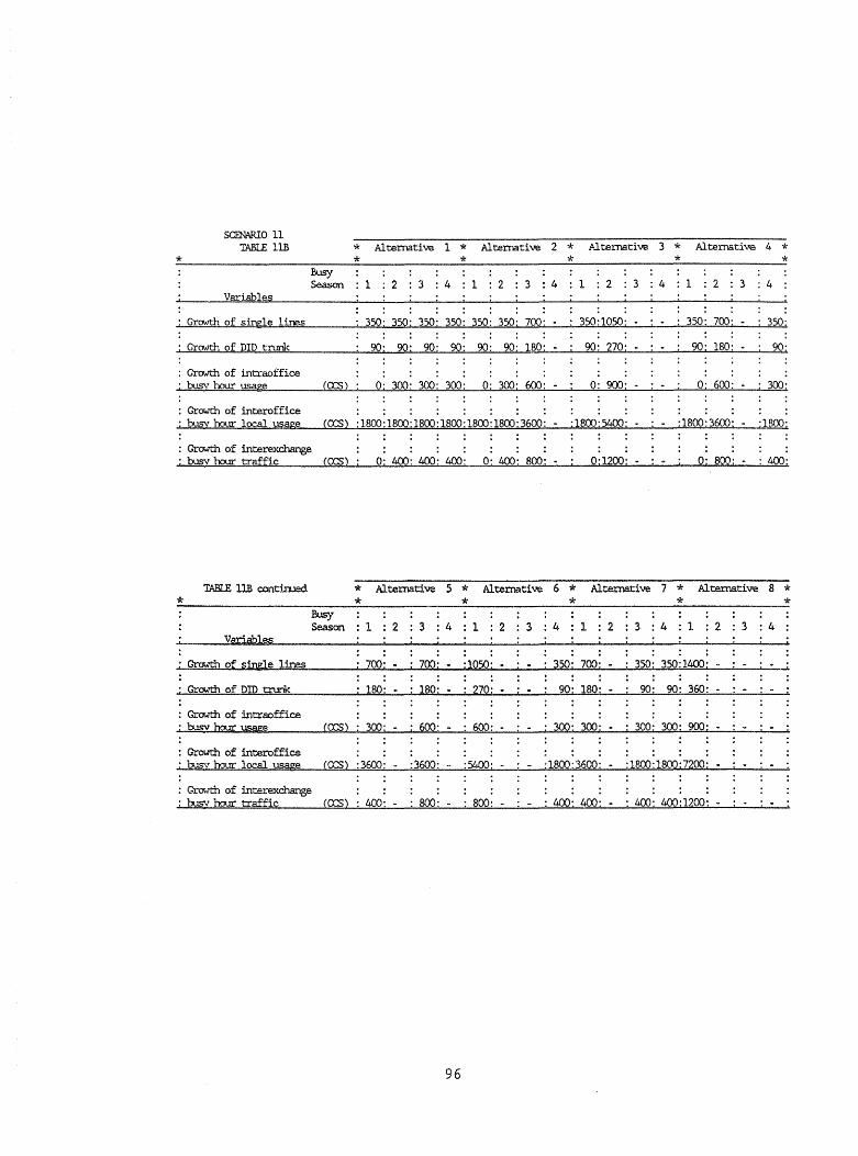
*
SCENARlOll TABlE IlB
Busy
* Alternative 1 * Alternative 2 * Alternative 3 * Alternative 4 * * * * * *
Season 1 2 3 : 4 1: 2 3 : 4 1 2 3 : 4 : 1 2 3: 4 Variables
: GrCMth of single lines 350' 350: 350' 350: 350: 350: 700: 350:1050; 350: 700: . 350:
; GrCMth of DID trunk 90: 90: 90: 90: 90: 90: 1~0; 90: 270' 90' , 180: 90' ,
: GrCMth of intraoffice 0' 300: 300' 300: O· 300' 600; 0: 900' 0' 600: Q 300' ! , ! , , , busy hour usage ( <XS)
; GrcM:h of interoffice : busy hour local usage (<XS) :1800:1800:1800:1800:1800:1800:3600: - :1800:5400:· - :1800:3600: - :1800:
: GrcM:h of interexchange : busy hour traffic (<XS) 0; 400: 400: 400; 0' 400: 800; 0'1200: 0: 800: : 400:
TABLE 1lB cont:irued * Alternative 5 * Alternative 6 * Alternative 7 * Alternatiw 8 * * * * * * *
Busy Season : 1 : 2 : 3 : 4 : 1 2 3 : 4 1 2 : 3 : 4 :1 : 2 3 : 4
.. Variab1~
, Growth of single lines , 700: 700: :1050: 350: 700; - 350: 350:1400' -: : : :
, Growth of DID trunk 180: 180: . 270; 90' 180' - 90: 90: 360: . , ,
: GrcM:h of intraoffice ; busy hour usage (<XS) 300' 600' 600: 300: 300' 300: 300' 900: -, , ,
: Growth of interoffice : : : busy hour local usage (<XS) :3600: :3600 :5400: '1800:3600; : 1800: 1800: 7200: .
: Growth of interexchange : busy hour traffic (<XS) 400: : 800 800: 400: 400: : 400: 400:1200: -
96
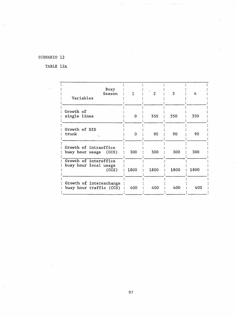
SGENARIO 12
TABLE 12A
Busy Season 1 2 3 4
Variables
Growth of single lines 0 350 350 350
Growth of DID trunk 0 90 90 90 ,
Growth of intraoffice busy hour usage (GGS) 300 300 300 300
Growth of interoffice busy hour local usage
(GGS) 1800 1800 1800 1800
Growth of interexchange busy hour traffic (eGS) 400 400 400 400
97

*
SCffiARIO 12 TABLE 12B
Variables
: Growth of single lines
: Growth of DID trunk
: erowt:h of intraoffice : bo.J.ay hour usage
: GrCMth of interoffice
* Alternative 1 * Alternative 2 * Alternative 3 * Alternative 4 * * * * * *
Busy Season : 1 2 3 : 4 1 2 3 : 4 : 1 : 2 3 : 4 1 : 2 3 : 4
O' 350: 350; 350; O' 350; 700; 0;1050- 0; 700; 350: - - -
0: 90: 90- 90: 0; 90; 180; 0: 270- 0: 180: 90:
(cx:s) 300: 300: 300: 300: 300- 300: 600: 300: 900; 300: 600: g 300 --
: busy hour local usage (o::::s) :1800:1800-1800:1800:1800:1800:3600: :1800:5400: :1800;3600: :1800;
: GrCMth of mterE!XChange : busy hour traffic (cx:s) : 400: 400: 400: 400: 400: 400- 800: ; 400:1200: 400: 800:· : 400~
TABLE l2B contirued
* Busy
* Alternative 5 * Alternative 6 * Alternative 7 * Alternative 8 * * * * * *
Season 1 2 3:4:1:23:412 3 : 4 1 : 2 3 : 4 Variables
: Growth of single lines 350: - : 700: : 700: 350: 350: . 350: 350:1050: -: Growth of DID trunk 90: : 180: : 180: 90: 90: - 90: 90: 270:
: GrCMth of intraoffice : busy hour USage (cx:s) 600: - : 600: 900: 300: 600: . 300: 300:1200: .
: GrOW'f.il of interoffice : : busy hour local usage <cx:s) :3600: . :3600: :.5400: : 1800: 3600: :1800:1800:7200: -
Growth of interexchange busy hour traffic (cx:s) 800: 800: :1200: : 400: 800 : 400 400:1600:
98

SCENARIO 13
TABLE 13A
Busy Season 1 2 3 4
Variables
Growth of single lines 350 350 350 350
Growth of DID trunk 0 90 90 90
Growth of intraoffice busy hour usage (CCS) 300 300 300 300
Growth of interoffice busy hour local usage
(CCS) 0 1800 1800 1800
Growth of interexchange busy hour traffic (CCS) 0 400 400 400
99

'*
SCENARIOl3 T.tilllE l3B
Variables
: Growth of single lines
: GrCMth of DID trunk
: G-row1::h of intraoffice : bJsy hour ysage
: Growth of interoffice : bJsy hour local usage
: Growth of interexchange
* Alternative 1 * Alternative 2 * Alternative 3 * Alternathwe 4 * * * * * *
Busy Season 1 2 3 : 4 : 1 2 3 : 4 1 2 3 : 4 1 2 3 : 4
350' 350: 350: 350: 350: 350: 700; 350;1050: 350: 700: 350; , - , - - ,
0- 90- 90: 90: 0: 90 : lBO' 0: 270; 0: 180: 90:
( CX::S) 300 : 300' 300' 300 ' 300 : 300 - 600 : 300: 900' 300: 600; 300;
(OCS) :1800;1800'1800:1800:1800:1800;3600: ; 1800: 3600: :1800:
; 00sy hour traffic (D:S) 0; 400; 400; 400: 0: 400; 800: 0:1200: 0: 800: ; 400;
TABLE DB contirued * Alternative 5 '* Alternative 6 '* Alternative 7 * Altemati ve 8 '* '* '* '* * '* * Busy
Season 1 2 3 :4 : 1 : 2 3 : 4 1 : 2 3 :4 : 1 : 2 : 3 :4 .. Variables
: : GrCMth of sim;le lines 700: - 700: :1050: ~50: 700: 350; 350:1400: -: GrCYWth of DID trunk 90: 180: 180: 90; 90: 90: 90: 270: -; Growth of intraoffice : hlsv hour ~e {CX::S} 600: 600: 900: 300: 600: 300: 3OO:l200: -: Growth of interoffice : ~ hour local usage ecx::s) :3600: :3600: 54CX): : 1800: 3600: - : 1800: 1800: 7200: -
: GrCMth of interexchange ; busv hour traffic (D:S) 400 - 800 - 800 - 400 400: : 400 400 1200: -
100

SCENARIO 14
TABLE 14A
Busy Season 1 2 3 4
Variables
Growth of single lines 0 350 350 350
Growth of DID trunk 90 90 90 90
Growth of intraoffice busy hour usage (CCS) 300 300 300 300
Growth of interoffice busy hour 10.ca1 usage
(CCS) 1800 1800 1800 1800
Growth of interexchange busy hour traffic (CCS) 0 400 400 400
101
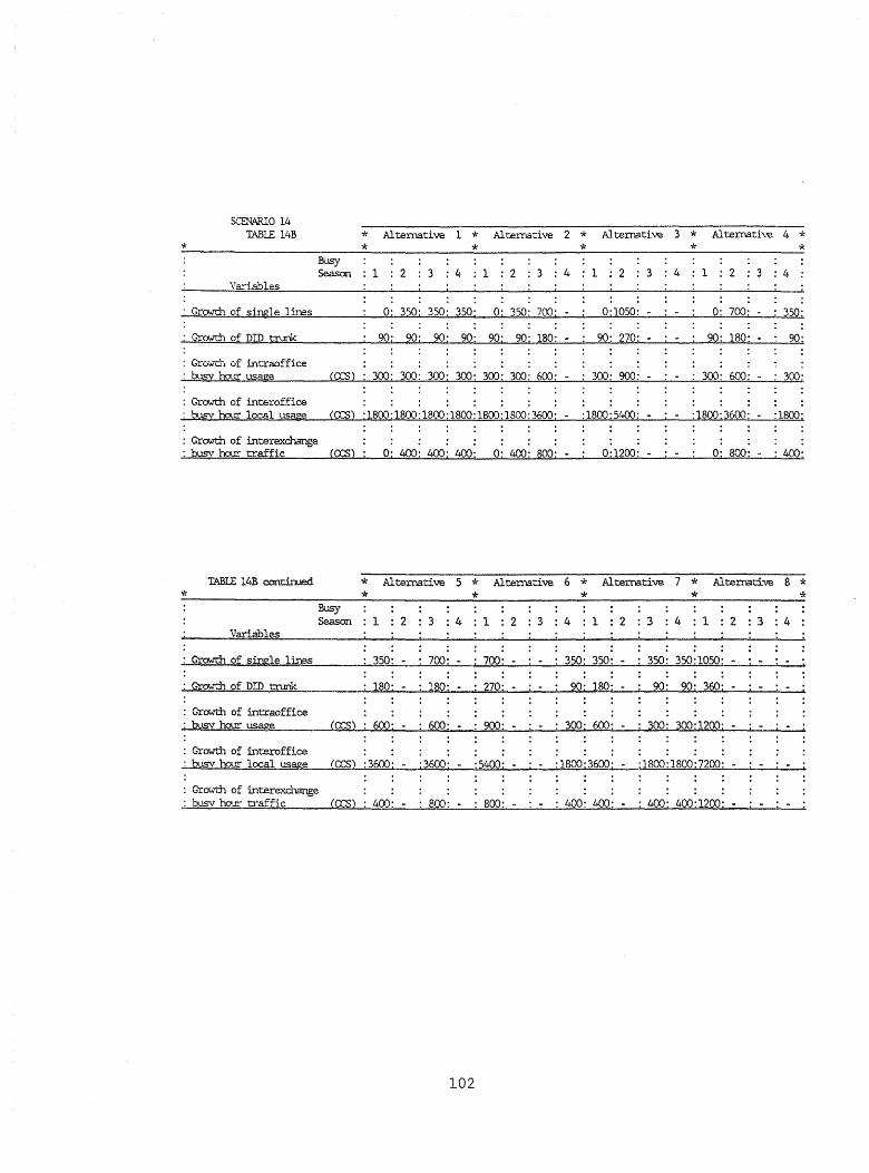
'*
SCENARIO 14 TABLE 14B
\Iariables
: Growth of single lines
: Growth of DID trunk
: Grcrw-u.' of intraoffice : bu§y hour usage
: Growth of interoffice : busv hour local usage
: Growth of intere.xchange
* Alternative 1 * Alternative 2 * Alternative 3 * Alternative 4 * * * * * *
Busy Season : 1 2 3:41:23:4 1 2 3 : 4 1 2 3 : 4
0: 350: 350: 350: 0: 350: 700: 0:1050: 0: 700: 350:
90; 90: 90: 90- 90: 90: 180: 90- 270: 90: 180: 90;
(CCS) 300- 300: 300- 300- 300: 300: 600: 300: 900: 300: 600- 300-,
(CCS) : 1800:1800:1800: 1800-1800: 1800: 3600: :1800:5400: - : 1800: 3600: :1800-
: buS'\' hour traffic (CCS) 0; 400: 400; 400: 0; 400: 800: 0:1200: - O' 800: - : 400:
TABLE 14B continJed * Alternative 5 '* Alternative 6 '* Alternative 7 * Alternative 8 * '* * * * '* *
Variables
: Growth of single lines
: Gro..'t:h of DID trunk
: Growth of intraoffice : busv hour usage
Busy Season
(o:s)
1 :
"
350:
: 180:
600:
2 3 : 4 : 1 :
700: 700:
- 180: : 270:
600: : 900:
: Growth of interoffice : busv hour local usage (CCS) :3600: - :3600: :5400:
: Growth of interexchange : busv oo.rr traffic (CCS) : 400: 800 - 800:
102
2 : 3 : 4 : 1 : 2 3 : 4 : 1 : 2 : 3 : 4
: 350: 350: 350: 350:1050:
90: 180: 90: 90: 360: -
300: 600: 300: 300:1200: -
- :1800:3600: - :1800:1800:7200:-
: 400: 400: : 400 400:1200: -
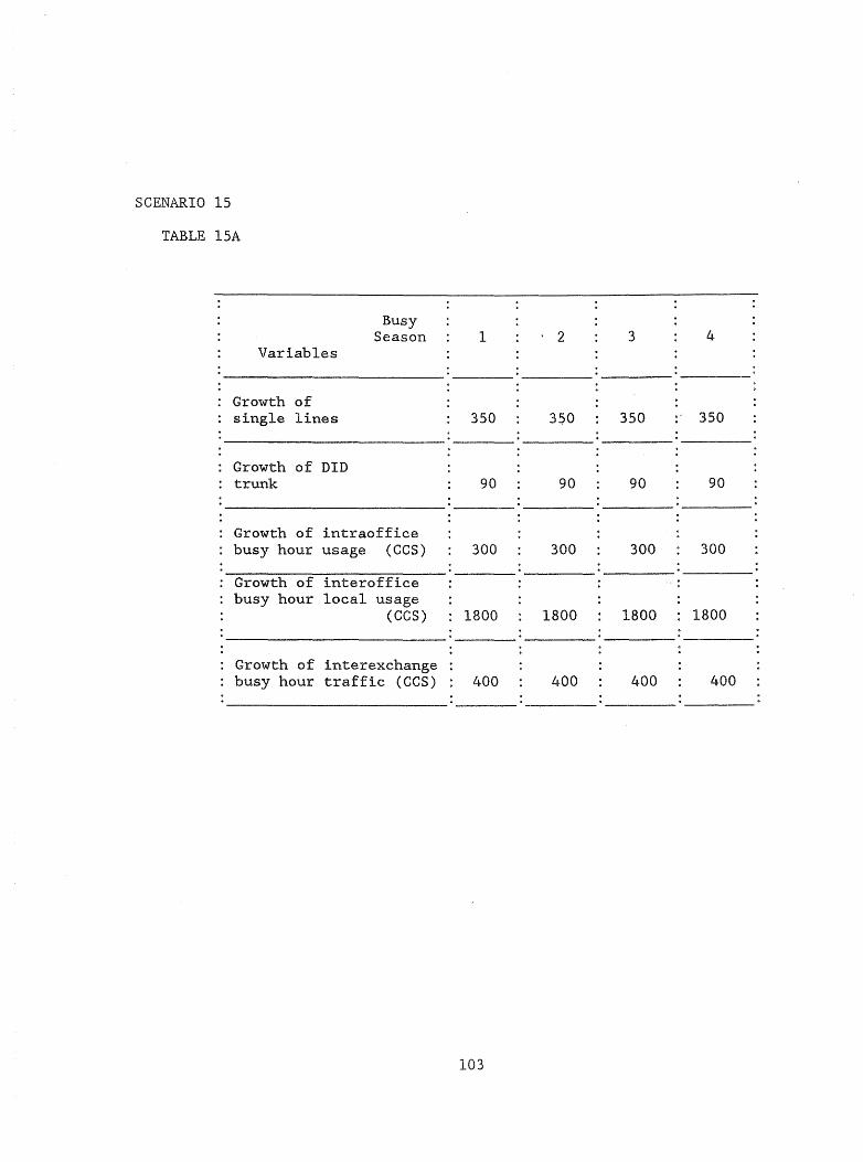
SCENARIO 15
TABLE l5A
Busy Season 1 \ 2 3 4
Variables
Growth of single lines 350 3~0 350 350
Growth of DID trunk 90 90 90 90
Growth of intraoffice busy hour usage (CCS) 300 300 300 300
Growth of interoffice busy hour local usage
(CCS) 1800 1800 1800 1800
Growth of interexchange busy hour traffic (CCS) 400 400 400 400
103
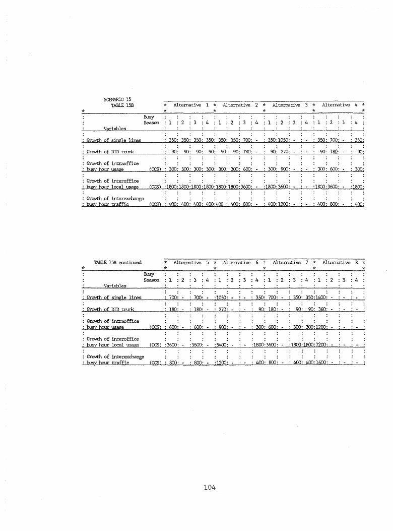
*
SCENARIO 15 TABLE 15B * Alternative 1 * Alternative 2 * Alternative 3 * Alternative 4 *
* * * * * Busy Season 1 2 3 : 4 1 2 3 4 1 2 3 : 4 1 2 3 : 4
Variables
; Growth of single lines
; Growth of DID trunk
; GrO'_·Jt.'I) of il1traoffice . busy hour usage
: Growth of interoffice ; busy hour local usage
: Growth of interexchange : busy hour traffic
TABLE l5E condIued
*
350: 350: 350: 350- 350; 350: 700:
90: 90: 90: 90: 90: 90: 1'80:
(a::s) 300: 300- 300' 300: 300: 300: 600-
(a::s) ;1800:1800-1800;1800-1800:1800-3600:
. ". . • It. • (a::s) ; 400- 1m- 400' 400;400 ; 400: 800;
* Alternative 5 * Alternative
* * Busy
350:1050: 350: 700: -
90- 270: 90: 180:
300: 900; 300: 600'
:1800:3600: : 1800: 3600-
- 400:1200; - ; 400: 800:
6 * Alternative 7 * Alternative
* * Season : 1 : 2 3 ; 4 : 1 : 2 : :> :4 : 1 2 : 3 :4 : 1 : 2 : :3
Variables
: Growth of single lines : 700: - 700: :1050: 350: 700: - 350: 350:1400: -:
: Growth of DID trunk 180: 180: 270: 90: 180: 90' 90: 360:
: Growth of intraoffice : busv hour usage (CCS) 600: 600- 900: 300: 600: ; 300- 300:1200: -,
: Growth of interoffice : busv hour local usage (CXS) :3600: :3600: :5400: :1800:3600: : 1800: 1800: 7200: -: Growth of interexchar!ge : busv hour traffic (D:S) 800: 800: :1200: : 400: 800: : 400: 400:1600: -
104
350:
90;
300 -,
:1800;
400 · ,
8 * *
: 4

SCENARIO 16
TABLE l6A
Busy Season 1 2 3 4
Variables
Growth of single lines 0 350 350 350
Growth of DID trunk 0 90 90 90
Growth of intraoffice busy hour usage (CCS) 0 300 300 300
Growth of interoffice busy hour local usage
(CCS) 0 1800 1800 1800
Growth of interexchange busy hour traffic (CCS) 400 400 400 400
105

*
SCENARIO 16 TABLE 16B
Busy
* Alternative 1 * Alternative 2 * Alternative 3 * Alternative 4 * * * * * *
Season 1 2 3 : 4 123:4:1 2 3 : 4 1 2 3 4 Variables
: Growth of sirn::1e lines
: Growth of DID trunk
: Growth of intraoffice : busv hour usage
: Growth of interoffice ; busv hour local usage
: Growth of int.erexchange
0: 350: 350: 350: 0: 350: 700:
0: 90: 90: 90: 0: 90- 180:
0: 300: 300: 300: 0: 300: 600:
(CXS) 0:1800:1800:1800: 0:1800:3600:
0:1050: 0: 700: 350:
0: 270: 0: 180; 90 -I
0: 900: 0: 600: 300-
0:3600: :1800-
; busv hour traffic (CXS) : 400: 400: 400: 400: 400: 400: 800: : 400:1200: : 400: 800: : 400:
TABLE 16B continued
* Busy
* Alternative 5 * Alternative 6 * Alternative 7 * Alternative 8 * * * * * *
Season 1: 2 3 : 4 : 1 : 2 3 : 4 : 1 2 3 : 4 : 1 2 3 : 4 Variables
: Growth of single lines 350: : 700: 700' 350: 350- 350: 350:1050:
, Growth of DID trunk 90: 180: 180: 90: 90' 90: 90: 270: --
: Growth of intraoffice : busv hour usage (CCS) 300: 600: 600: 300: 300: 300: 300: 900: .
: GrowtfJ. of interoffice : busv hour local usage (CCS) ;1800: :3600: :3600: :1800:1800: :1800:1800:5400:
: Growth of interexchange : bu.§y hour traffic (CCS) 800: 800 - 1200: : 400: 800: 400: 400 1600
106
APPENDIX B
24-1F&\CTIONAL FACTORIAL EXPERIMENTAL CONSTRUCTION PLAN PROJECT NA}lE: MARGINAL COST OF PLAIN OLD TELEPHONE SERVICE (POTS)
by
Clark A. Mount-Ca.mpbell Associate Professor of Industrial and
Systems Engineering
Hisham M. Chouoiki Graduate Research Associate
THE NATIONAL REGULATORY RESEARCH INSTITUTE Columbus, Ohio
September, 1986
107

In a 24 - 1 fractional factorial experimental design, eight observations
(treatment combinations or scenarios) are required. These observations are
selected from a full 24 factorial design according to the defining equation.
I = ABeD. The eight observations (scenarios) are listed in the tables of
this appendix that are labeled xA where x is the scenario number.
Eight four-year construction programs are possible to satisfy the
demand requirements specified in a given scenario. These are given in
tables with labels xB where again, x is the scenario number. For example,
the eight alternatives specified for scenario 1 are listed in table lB.
Similarly, the alternatives for scenarios 2, 3, 4, 5, 6, 7 and 8 are listed
in tables 2B to 8B, respectively.
The tables of this appendix are given in the same format as the actual
data request shown at the end of appendix A in the exhibit 1.
108
SCENARIO 1
TABLE lA
Year 1 2 3 4 Variables
==== ........... ------------------: --------: --------: --------: --------
Single lines added
DID Trunks added
Intraoffice usage added (CCS)
Interoffice local added (CCS)
o
o
o
o
109
350 350 350
90 90 90
300 300 300
1800 1800 1800
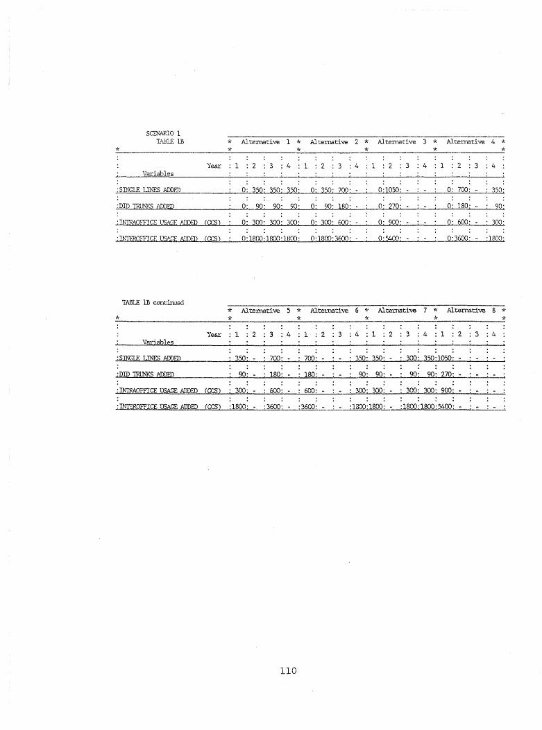
SCENARIO 1 T.A.blE lB
* Year
Variables
: S IN,;LE lTh"'ES ADDED
: DID 1RUNKS ADDED
: ThrrRAOFt""ICE USAGE ADDED !O:S}
: L\"TEROITICE US.A.GE ADDED (O:S:l
TABLE lB contirued
* Year
Variables
: SIJ'iGLE I...:mES ADDED
; DID 'ffiIJNKS ADDED
.,;IN'IRAOFflCE USAGE ADDED (CCS)
* Alternative 1 * Al ternati ve 2 * Alternative 3 * Alternative 4 * * * * * *
1 2 3 4 1 2 3 :4 1 2 3 4 1 2 3 :4
0: 350: 350: 350: 0: 350: 700: 0:1050: 0: 700: 350:
0: 90: 90: 90: 0: 90: 180: 0: 270: 0: 180: 90:
0: 300: 300: 300: 0: 300: 600: 0: 900: 0: 600: 300:
0:1800:1800:1800: 0:1800-3600: 0:5400: 0:3600: :1800:
* Alternative 5 * Alternative 6 * Alternative 7 * .IUternative 8 * * * * * *
1 2 :3 : 4 1 2 3:4 1 2 3 : 4 : 1 2 : 3 : 4
350; 700; 700: 350: 350: - 300: 350:1050: -
90: 180: 180: 90: 90:- 90: 90' 270: -
300: 600: 600: 300: 300: 300: 300 900: -
..;.Th'fJ.'EROFfICE USAGE ADDED (CXS) :1800: :3600: - :3600: :1800:1800: - :1800:1800 5400: -
110

SCENARIO 2
TABLE 2A
Year 1 ,2 3 4 Variables
: -------------------------: --------: --_ .... _---: --------: --------
Single lines added
DID trunks added
Intraoffice usage added (CGS)
Interoffice local added (GGS)
350
o
o
1800
III
350 350 350
90 90 90
300 300 300
1800 1800 1800
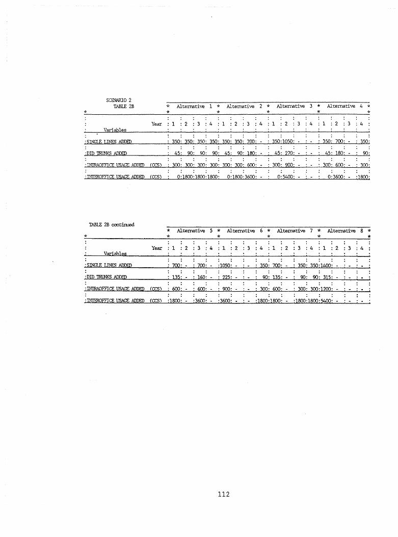
*
SCENARIO 2 TABLE 2B
Variables
: SINGLE LINES ADDED
:DID TRUNKS ADDED
Year
: ThrrEROFFICE USAGE ADDED ( CX;S)
TABLE 2B contin.led
*
* Alternative 1 * Alternative 2 * Alternative 3 * Alternative 4 * * * * * *
1 2 3 : 4 1 2 3 : 4 1 2 3 4 1 2 3 : 4
350: 350: 350: 350: 350: 350; 700; 350:1050: 350: 700; 350;
45: 90: 90: 90; 45: 90- 150: - 45: 270: 45: 180: 90:
300~ 300; 300: 300: 300: 300: 600: 300: 900: 300: 600: 300;
0:1800:1800:1800: 0:1800:3600: 0:5400: 0:3600: :1800;
* Alternative 5 * Alternative 6 * Alternative 7 * Alternative 8 * * * * * *
Year 1 2 3:4:123:4:1 2 3 : 4 : 1 : 2 : 3 : 4 Variables
: : Sm:;u: I..INF:? ADDED 700' - - 700' - -1050: 350- 700' - 350' 350:1400: -
: : DID 'IRUNKS ADDSD 135: - 160: - : 225: 90- 135: - 90: 90: 315: -
: : :mrRAOF'F1CE USAGE ADDED (CX;S) 600' - 600 : 900: 300: 600: 300' 300:1200:
: Th'1'EROF'F1CE USAGE ADDED (CX;S) 1800: - :3600 - :3600: :1800:1800: - : 1800: 1800: 5400:
112

SCENARIO 3
TABLE 3A
Year 1 2 3 4 Variables
------------------------- -------- -------- -------- --------
Single lines added 0 350 350 350
DID trunks added 90 90 90 90
Intraoffice usage added 0 300 300 300 eCCS)
Interoffice local added 1800 1800 1800 1800 eCCS)
113

'*
SClliARIO 3 TABLE 3B
Variables
: SIN:;lE ill'ES ADDED
: DID 'IRl.lNKS ADDED
Year
: 1:-lRA,.OmCE USAGE ADDED (OCS)
* Alternative 1 * Alternative 2 * Alternative 3 * Alternative 4 * * * * * *
1 2 3 : 4 1 2 3 : 4 1 2 3 : 4 1 2 3 : 4
350: 350: 350: 350: 350: 350: 700: :350 :1050: 350: 700- 350;
45: 90: 90: 90: 45: 90: 180: : 45 270: 45: 180: 90-t
0: 300: 300- 300- 0: 300: 600: : 0 : 900: 0: 600: - : 300:
·l.~":"EROmCE USAGE ADDED (OCS) :1800:1800:1800:1800:1800:1800;3600; :1800:5400: - :1800:3600: :1800:
TABLE 3B cont:i.n.led
* Alternative 5 * Alternative 6 * Alternative 7 * Alternative 8 * * * * * * *
Year 1 : 2 3 : 4 : 1 2 3 :4 1 2 3 :4 : 1 : 2 : 3 : 4 Va.-ri.ables
: ; Sm:;u: lINES ADDED 700: 700; :1050: 350: 700: 350- 350:1400'
: : DID 'IRlJI'ia<S ADDED 155: Q 190- 225: 90: 135: ~ 90- 90: 315: -,
: Th"IRAOFFICE USAGE ADDED (OCS) 300: 600: 600: 300- 800- - 300: 300- 900: .
: : : : : '.rmROFFICE USAGE fm.ED (OCS) 3600; 3600- ;5400: :1800-3600- - : 1800: 1800: 7200: -
114
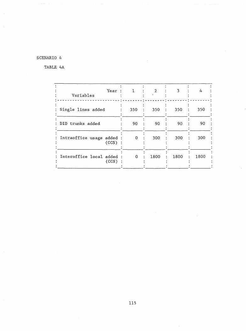
SCENARIO 4
TABLE 4A
Year 1 2 3 4 Variables
: -------------------------: --------: --------: --------: --------
Single lines added
DID trunks added
Intraoffice usage added (CCS)
Interoffice local added (CCS)
350
90
o
o
115
350 350 350
90 90 90
300 300 300
1800 1800 1800

*
SCENA.R.IO 4 TABLE 4B
Variables
: Snr;LE LINES ADDED
: DID !ffiUNKS ADDED
Year
1rv"C'\ \\.AA:>/
; Th'TEROFFICE USAGE ADDED (cx::s)
TABLE 4B cont:inJed
* Year
Vari@les
: Sm:;u: lJNES ADDED
; DID 'lRIJNKS ADDED
: mIRAOFFICE USAGE ADDED (CXS)
: Th"TEROFFICE USAGE ADDED (OCS2
* Alternative 1 * Alternative 2 * Alternative 3 * Alternative 4 * * * * * *
1 2 3 : 4 1 2 3 : 4 1 2 3 : 4 1 2 3 : 4
350: 350: 350: 350: 350: 350; 700; 350:1050; 350; 700; 350;
90' 90' 90: 90: 90' 90: 18'0: 90: 270: - 90' 180: - 9O~ . , . . 0: -:tN'l,
J ! 300: 300: 0: 300' 600~ 0: 900: - 0: 600: 300; --
0:1800:1800:1800' 0:1800:3600: 0:5400: - 0:3600: - :1800;
* Alternative 5 * Alternative 6 * Alternative 7 * Alternative 8 * * * * * *
1 2 3 : 4 : 1 2 3 : 4 :1 2 3 :4 : 1 2 3 : 4
700; 700: :1050; 350: 700: - 350; 350:1400: -180: 180: : 270; 90: 180: - 90: 90: 300' -
: 300: 600: 600' 300: 300: 300: 300: 900 -,
: : 1800: - :3600; - 3600; - :1800'1800: - : 1800: 1800: 5400 -
116

SCENARIO 5
TABLE 5A
Year 1 2 3 4 Variables
------------------------- -------- -------- -------- --------
Single lines added 0 350 350 350
DID trunks added 0 90 90 90
Intraoffice usage added 300 300 300, 300 (CCS)
Interoffice local added 1800 1800 1800 1800 (CCS)
117

*
S~05
TABLE 5B
Variables
: DID 1RlJNKS ADDED
Year
·IN1RA.Omcr PSA..GE ADOrn (D::S)
* Alternative 1 * Alternative 2 * Alternative 3 * Alternative 4 * * * * * *
1 2 3 : 4 1 2 3 4 1 2 3 : 4 1 2 3 : 4
0: 350: 350: 350: 0: 350: 700: 0 :1050: 0: 700: 350;
0: 90: 90: 90: 0: 90: 180; 0 ; 270; 0: 180; 90' ,
300; 300; 300: 300: 300: 300; 6QO: 300' 900' , 300: 600: -:~
~'TEROmCE VSAGE ADDED (cx::s) : 1800: 1800: 1800: 1800: 1800: 1800: 3600: :1800;5400; : 1800:361.JO: :lROO~
TABLE SB <lOI1t:i.rued
* Alternative 5 * Alternative 6 * Alterl1ative 7 * Alternative 8 * * * * * ----------*---------------!
Year : 1 2 3 : 4 : 1 2 3 : 4 : 1 :2 3 :4 : 1 2 3 : 4 Variables'
: Sm:;LE lJNES ADDED : 350' 700; : 700: 350: 350: 350: 350:1050: -: DID 'IRIN<S ADDED 90: 180: 180: 90' , 90' , 90: 90: 270:
: Th"IRAOFFTCE USAGE ADDED (en;) 600- 600: 900 300: 600: ~ 300: 300:1200: -: Th'TEROFF1CE USAGE ADDED (en;) :3600: :3600: :5400 1800:3600: - 1800:1800:7200: -
118

SCENARIO 6
TABLE 6A
Year 1 2 3 4 Variables
-- - -- --- --- --- - -- ---- ---- -------- -------- -------- --------
Single lines added 350 350 350 350
DID trunks added 0 90 90 90
Intraoffice usage added 300 300 300 300 eCCS)
Interoffice local added 0 1800 1800 1800 eCCS)
119

"*
SCENARIO 6 TABLE 6B "* Alternative 1 "* Alternative 2 "* Alternative 3 * Alternative 4 *
* "* * * * Year 1: 2 3: 4 1: 2 3: 4 1 2 3:412:3:4
Variables
: STInE LThTES ADDED
:DID'lRUNYS ADDED
: Th'IRAOfl1CE llSAGE ADDED (CCS)
-nn1ROfl1CE pSAGE ADDED (CCS)
ThBI..E 6B continJed
* * *
Year Variables
: Sm:;tE llNES ADDED
: DID 'IRIJNKS ADDED
lliIRAOFfICE USAGE ADDED (CCS)
Th'TEROFFICE USAGE ADDED (CCS)
350: 350: 350: 350: 350: 350: 700:
0: 90: 90: 90: 0: 90-I 180:
300: 300: 300: 300: 300: 300: 600:
0-1800:1800:1800: 0:1800:3600:
Alternative 5 * Alternative 6 * * *
1 : 2 3 : 4 : 1 : 2 : 3 : 4 :
700: : 700: :1050: : 350-
90: , 180: - 180: 90'
350:1050:
0: 270:
300: 900:
0:5400:
Alternative 7 * *
1 2 3 : 4 :
350: 700: 350:
0: 180: - 90-!
300: 600: - 300;
0:3600: :1800-
Alternative 8 * *
1 : 2 : 3 : 4
700: 350: 350:1400: -:
90: 90' 90: 270: . -
600: : 600' 900: 300:600 : 300: 300 1200: . - -
1800: :3600: :3600: : 1800: 1800: 1800: 1800 5400: -
120

SCENARIO 7
TABLE 7A
Year 1 2 3 4 Variables
------------------------- -------- -------- -------- --------
Single lines added 0 350 350 350
DID trunks added 90 90 90 90
Intraoffice usage added 300 300 300 300 (CCS)
Interoffice local added 0 1800 1800 1800 .. (CCS)
121

*
SCENt\RIO 7 TABLE 7B
Variables
: S~ LINES ADDED
: DID TRUNKS ADDED
Year
: IN'IRAOFF1CE U5.t>,GE ADDED (CCS)
: INTEROFF1CE USAGE ADDED (CCS)
T.A.BLE 7B contirued.
*
* Alternative 1 * Alternative 2 * Alternative 3 * Alternative 4 * * * * * *
1 2 3 412 3 : 4 1 2 3 4 1 2 3 : 4
0: 350: 350: 350: 0: 350: 700: 0:1050: 0 700: 350:
90' ! 90: 90: 90: 90: 90: 180: 90: 270: 90: 180: 90:
300' 300: 300: 300: 300: 300: 600: . 300: 900' - 300; 600: - 300' ! !
0:1800:1800:1800: 0:1800:3600; - 0:5400; - 0:3600: :1800:
* Alternative 5 * Alternative 6 * Alternative 7 * Alternative 8 * * * * * *
Year 1: 2 3 : 4 : 1 2 3 : 4 : 1 : 2 : 3 : 4 : 1 : 2 : 3 : 4 Variables
: : : Sm:;u: LJNES N$)FD 350: 700- . 700: 350: 350: 350: 350:1800:
: : ! 180' - . 270- - 90: 180: - 90- 90; 360; -; DID TRUNKS ADDED 180: -
: : : :IN':rnAOFF1CE USAGE ADDED (CCS) 600: 600: 900-. 300- 600- 300 300 1800:
: : : :Th"TEROmCE USAGE @DED (cx:s) :1800:- :3600: - :3600: - - :1800:1800: - : 1800 1800 5400: -
122
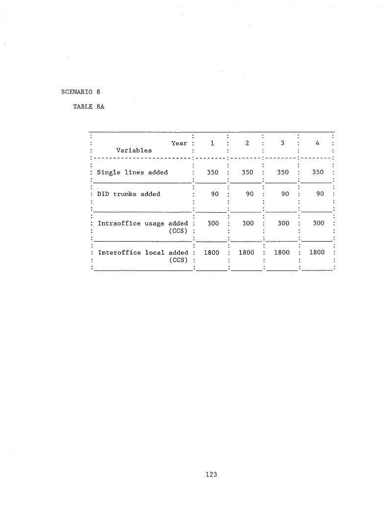
SCENARIO 8
TABLE 8A
Year 1 2 3 4 Variables
-------------------------: --------: --------: --------: --------
Single lines added
DID trunks added
Intraoffice usage added (CCS)
Interoffice local added (CCS)
350
90
300
1800
123
350 350 350
90 90 90
300 300 300
1800 1800 1800
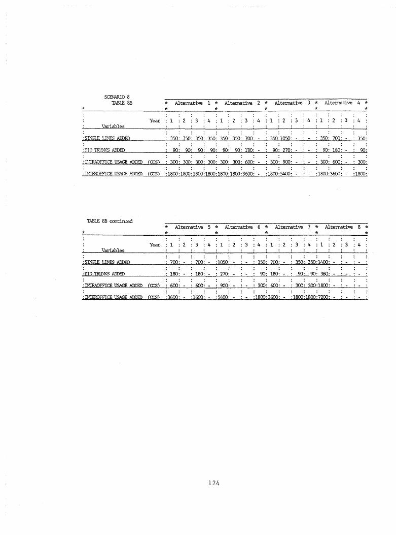
*
SCENARIO 8 TABlE 8B
Variables
: sm::;u: LINES ADDrn
:DID TRIJNKS ADDED
* Alternative 1 * Alternative 2 * Alternative 3 * Alternative 4 * * * * * *
Year 1 2 3: 4 : 1 2 3: 4 1: 2 3: 4 : 1 2: 3 : 4
350: 350: 350: 350: 350: 350: 700: 350:1050: 350: 700: . 350:
90: 90: 90: 90: 90: 90: 1'80: 90: 270: 90: 180: 90:
..;.!'iIRAOffiCE USAGE ADDrn (0:5) 300: 300' 300: 300: 300' 300: 600: 300: 900: 300: 600: 300'
: ThTIROffiCE USAGE ADDED (0:5) :1800-1800:1800:1800:1800:1800:3600: : 1800: 5400: : 1800: 3600: - :1800-
TABlE 8B contirued
*
Variables
: sm::;u; l.JNES ADDED
• DID 'IRlJNKS ADDED
: Th"IRAOFF1CE USAGE ADDED
:ThTIROFF1CE USAGE ADDED
* Alternative 5 * Alternative 6 * Alternative 7 * Alternative 8 * * * * * *
Year : 1 : 2 : 3 : 4 : 1 : 2 : 3 : 4 : 1 : 2 : 3 : 4 : 1 : 2 : 3 : 4
: 700: . 700; :1050: 350: 700: 350:, 350: 1400: .
: 180' G 180' 270' 90' 180: . 90: 90' 360: . .
(o:s) 600: . 600 900: 300' 600; - 300: 300 1800; -. : :
(o:s) 3600: 3600 5400: 1800:3600: . :1800:1800 7200' -
124
APPENDIX C
Z3-1FRACTIONAL FACTORIAL EXPERIMENTAL CONSTRUCTION PLAN PROJECT NAME: MARGINAL COST OF PLAIN OLD TELEPHONE SERVICE (POTS)
by
Clark A. Mount-Campbell Associate Professor of Industrial and
Systems Engineering
Hisham M. Chouoiki Graduate Research Associate
THE NATIONAL REGULATORY RESEARCH INSTITUTE Columbus, Ohio
September, 1986
125
In a 23- 1 fractional factorial experimental design, four observations
(treatment combinations or scenarios) are required. These observations are
selected from a full 23 factorial design according to the defining equation
I = ACD. The four observations (scenarios) are listed in the tables of this
appendix that are labeled xA where x is the scenario number. Factor B is
held fixed in all scenarios thereby reducing the number of factors to 3.
Eight four-year construction programs are possible to satisfy the
demand requirements specified in a given scenario. These are given in
tables with labels xB where again, x is the scenario number. For example,
the eight alternatives specified for scenario 1 are listed in table lB.
Similarly, the alternatives for scenarios 2, 3 and 4 are listed in tables 2B
to 4B, respectively.
The tables in this appendix are given in the same format as the actual
data request shown at the end of appendix A in the exhibit 1.
126
SCENARIO 1
TABLE lA
Year 1 2 3 4 Variables
------------------------_. --------: --------: --------: --------
Single lines added
DID trunks added
Intraoffice usage added (CCS)
Interoffice local added (CCS)
o
45
o
o
350
90
300
1800
350 350
90 90
300 300
1800 1800
------------------------ ------- ------- ------- -------
127
-I<
SCENARIO 1 TABLE lB
Variables
! sm:;u: lJNES ADDED
:!)ID TRUNKS ADDED
Year
: T\'1RI\OFFICE USAGE ADDED (CCS)
: rmROFFICE USAGE ADDED (CCS)
TABLE lB conti.rued
* Year
Variables
; Sm::;r..E LrnES ADDED
; DIP 'IRUNKS ADDED
:Th"IRAOFFICE USAGE ADDED (o:::s)
: Th'TEROFTICE Us.q ADDED (CXS)
-I< Alternative 1 -I< Alternative 2 * Alternative 3 * Alternative 4 * * * * * *
1 2 3 : 4 1 2 3 4 1 2 3 4 1 2 3 : 4
0: 350: 350: 350: 0: 350: 700: 0:1050: 0--
700: 350:
45; 90- 90--
90: 0: 90' , 180; 45; 270; 45: 180: 90-I
0; 300-! 300: 300: 0: 300: 600: 0; 900: 0: 600: 300;
0:1800:1800:1800: 0:1800:3600: 0:5400: 0:3600; :1800;
* Alternative 5 * Alternative 6 * Alternative 7 * Alternative 8 * * * * * *
1 2 3:4:1:23 4 : 1 2 3 : 4 : 1 : 2 3 : 4
: : 350: 700: : 700: 350: 350' 300: 350:1050: -
: : : 135: . 180' 225: 90: 135' - 90' 90: 315: -! !
: : : : 300: 600 : 600: 300: 300: . 300: 300: 900: -
: : : : : : :1800: '3600 :3600: :1800:1800' : 1800: 1800; 5400' -
128

SCENARIO 1
TABLE 2A
Year 1 2 3 4 Variables
-------------------------: --------: --------: --------: --------
Single lines added
DID trunks added
Intraoffice usage added (CCS)
Interoffice local added (CCS)
350
45
300
o
129
350 350 350
90 90 90
300 300 300
1800 1800 1800

*
SCENo\RlO 2 TABLE 2B * Alternative 1 * Alternative 2 * Alternative 3 * Alternative 4 *
* * * * * Year 1: 2 3:4 1:2 3:4 1 2 :3:4 1 2 3 4
Variables
: Soo.? LINES ADDED 350: 350: 350; 350; 350: 350: 700: 350:1050: - 350: 700; 350;
; DID TRUNKS ADDED 45: 90' 90' 90' , 45: 90' 180: 45: 270' 45: 180: 90'
: n-,'rTIIAOFFTCE USAGE ADDED (CCS) 300: 300: 300: 300: 300: 300: 600: 300: 900: 300: 600: 300: :
; Th"TEROFFICE tJSAGE ADDED (CCS) 0'1800-1800:1800: 0:1800:3600: - 0'5400: 0:3600: - :1800:
TABlE 2B conti.rued
* * Alternative 5 * Alternative 6 * Alternative 7 * Alternative 8 * * * * * *
Year : 1 : 2 3: 4 : 1 : 2 3: 4 : 1 : 2 :3: 4 : 1 2 3 : 4 Variables
: Sm::;I.E LINES ADDED 700: . 700: :1050: . : 350: 700: 350: 350:1400: •
: DID 1RIJNKS ADDED 135: - 180: : 225: : 90: 135: 90: 90: 315: . .
'Th'IRAOFFICE USAGE ADDED (cx.:s) : 600: - : 600: ; 900: : 300: 600: - 300: 300:1200:
:ThTIROFFICE USAGE ADDED (cx.:s) :1800: - :3600: - :3600: - :1800:1800: - :1800:1800:5400:-
130
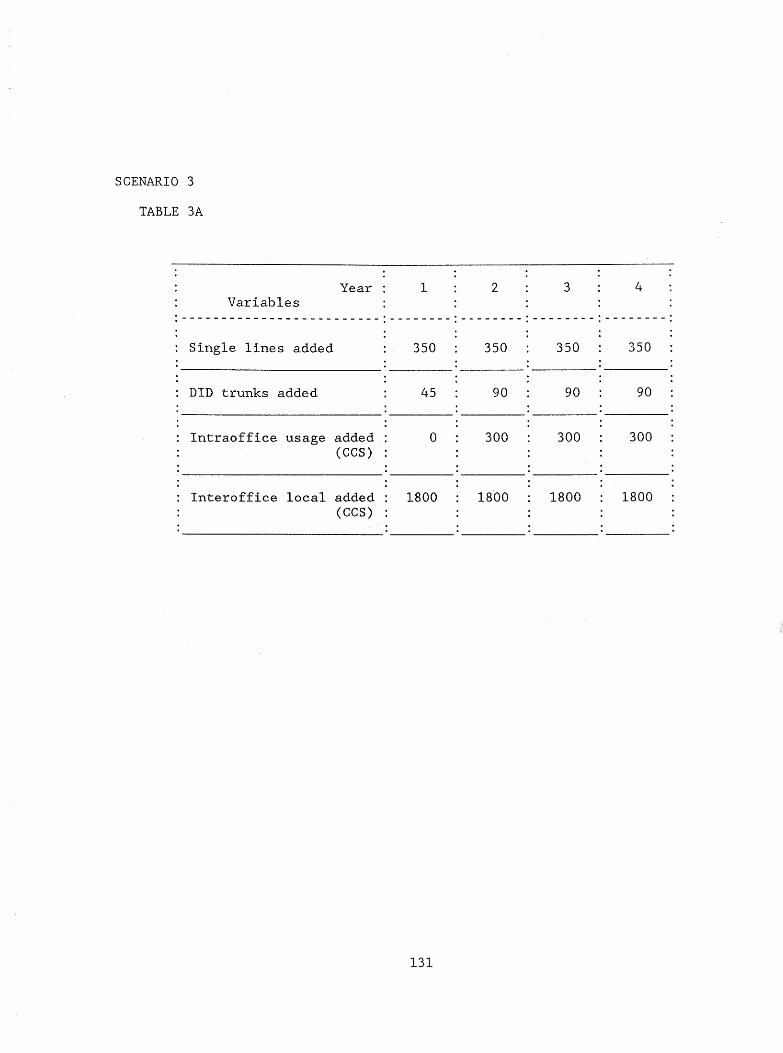
SCENARIO 3
TABLE 3A
Year 1 2 3 4 Variables
------------------------- -------- -------- -------- --------
Single lines added 350 350 350 350
DID trunks added 45 90 90 90
Intraoffice usage added 0 300 300 300 (CCS)
Interoffice local added 1800 1800 1800 1800 (CCS)
131

*
SCENARIO 3 TABLE 3B
Variables
: sm:;u:: lINES ADDED
;D1O 1Rl1NKS ADDED
* *
Alternative 1 * Alternative 2 * * *
Alternative 3 * Alternative 4 * * *
Year 1 2 3: 4 : 1 2 3: 4 : 1 2 3: 4 : 1 2 3 : 4
350: 350: 350: 350: 350: 350: 700: : 350 : 1050: 350: 700: • 350;
45- 90: 90' 90: 45: 90: 180: - 45 : 270: - 45: 180: - 90;
_: Th'TAAOFFICE USAGE ADDED (cx:s) 0: 300: 300; 300: 0: 300: 600: : 0 - 900: 0: 600: - 300;
: ThTIROFFICE USAGE ADDED (cx:s) :1800:1800:1800:1800:1800:1800:3600: - :1800:5400:- - :1800:3600: - :1800:
TABLE 3B contin.ro * Alternative 5 * Alternative 6 * Alternative 7 * Alternative 8 *
* * * * * * Year : 1 : 2 3: 4 : 1 : 2 : 3 : 4 1: 2 3: 4 : 1 : 2 3 : 4
Variables
; SIN;::;IE I..JNES ADDED : 700: . , 700: . :1050: . 350: 700: - 350: 350:1400: • :
: 135: . -
190: - : 225: -: DID 'IRUNK.S ADDED 90: 135: - : 90: 9O~ 315: -
:lNIRAOFFICE USAGE ADDED (o::s) : 300: - : 600:· • 600 300: 800: - - 300: 300: 900: . -. . : Th'TEROFFICE USAGE ADDED (o::s) -3600: - :3600: ~ :5400 - - :1800:3600: - :1800:1800:7200:-
132
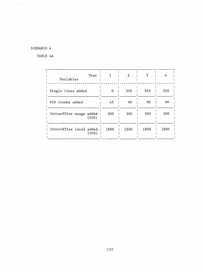
SCENARIO 4
TABLE 4A
Year 1 2 3 4 Variables
------------------------- -------- -------- -------- --------
Single lines added 0 350 350 350
DID trunks added 45 90 90 90
Intraoffice usage added 300 300 300 300 (CCS)
Interoffice local added 1800 1800 1800 1800 (CCS)
133

*
SCENARIO 4 TABLE 4B
Variables
: SINGLE 1...Th"'ES ADDED
: DID 'IRUNY-S ADDED
'ThTIROFFICE USAGE ADDED (CCS)
TABLE 4B continued
* Year
Variables
: SThGLE LINES .ADDED
: DID 'IRlJNKS ADDED
: Th"lRADFF1CE USAGE ADDED (CCS)
* Alternative 1 * Alternative 2 * Alternative 3 * Alternative 4 * * * * * *
1 2 3 : 4 1 2 3 : 4 1 2 3 4 1 2 3 : 4
0' ! 350; 350: 350- 350: 350: 700: 350:1050: 350: 700: 350; :
45: 90: 90: 90: 45: 90: 180: 45: 270: 45: 180: 90;.
0: 300: ~. 300: 0: 300: 600: 0: 900; 0' 600: 300: _ .......... ,
0;1800:1800;1800:1800:1800;3600; :1800' 5400' : 1800: 3600: ;1800'
'* Alternative 5 * Alternative 6 * Alternative 7 * Alternative 8 * * * * * *
1 : 2 3 : 4 1 : 2 3 : 4 1 2 3 : 4 : 1 2 3 : 4
350' 700; 700; 350: 350: 350: 350;1050: -180: 225: 90: 135: 0 90: 90' 315: 0 , , 135:
: 600; : 600: 900: 300: 600; - 300: 300:1200: -
: Th"I'EROFF1CE USAGE ADDED ( CCS) ; 3600: :3600: :5400: : 1800: 3600: : 1800: 1800; 7200: -
134
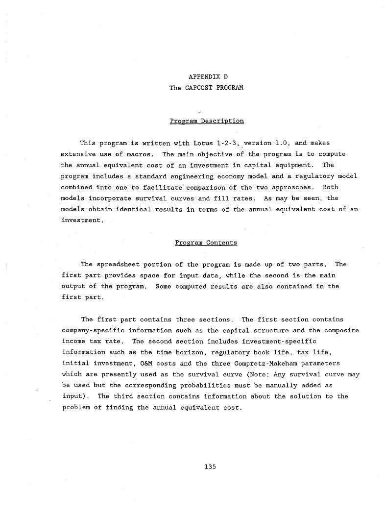
APPENDIX D
The CAPCOST PROGRAM
Program Description
This program is written with Lotus 1-2-3, version 1.0, and makes
extensive use of macros. The main objective of the program is to compute
the annual equivalent cost of an investment in capital equipment. The
program includes a standard engineering economy model and a regulatory model
combined into one to facilitate comparison of the two approaches. Both
models incorporate survival curves and fill rates. As may be seen, the
models obtain identical results in terms of the annual equivalent cost of an
investment.
Program Contents
The spreadsheet portion of the program is made up of two parts. The
first part provides space for input data, while the second is the main
output of the program. Some computed results are also contained in the
first part.
The first part contains three sections. The first section contains
company-specific information such as the capital structure and the composite
income tax rate. The second section includes investment-specific
information such as the time horizon, regulatory book life, tax life,
initial investment, O&M costs and the three Gompretz-Makeham parameters
which are presently used as the survival curve (Note: Any survival curve may
be used but the corresponding probabilities must be manually added as
input). The third section contains information about the solution to the
problem of finding the annual equivalent cost.
135

The specific cells for the three sections are defined as follows:
(Note: Capital letters denote spreadsheet columns and numbers denote
spreadsheet rows.)
Cell description for section 1:
E3 Percentage composed of debt E4 Average interest rate on debt E5 Percentage composed of equity E6 Average rate of return on equity E7 Composite cost of capital E8 Composite income tax rate
Cell description for section 2:
12 Time horizon 13 Initial amount invested 14 Regulatory book life IS Tax life 16 Method of tax depreciation used
1) Sum-of-years digits (SOYD) 2) Straight line (SL) 3) Double declining balance that switches to straight line
(DDB/SL) 4) Accelerated cost recovery system (ACRS)
17 O&M growth rate 18 O&M gradient change 19 O&M initial cost
Gompertz-Makeham parameters:
III s = 0.99 112 g 0.955 113 = c 1.4
Cell description for section 3:
DlO Lower bound of the interval that contains the solution D12 Upper bound of the interval that contains the solution D1l Midpoint of the interval D13 Width of the interval Ell Expected net present value of unrecovered investment E13 The final interval width required
136
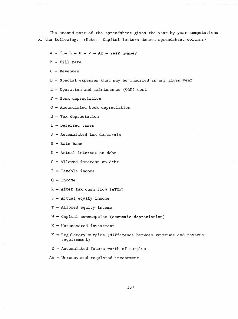
The second part of the spreadsheet gives the year-by-year computations
of the following: (Note: Capital letters denote spreadsheet columns)
A
B
C
D
E
F
G
H
I
J
M
N
o
p
Q
R
S
T
w
x
Y
z
AA
K = L = U v = AE Year number
Fill rate
Revenues
Special expenses that may be incurred in any given year
Operation and maintenance (O&M) cost ,
Accumulated book depreciation
Tax depreciation
Deferred taxes
Accumulated tax deferrals
Rate base
Actual interest on debt
Allowed interest on debt
Taxable income
Income
After tax cash flow (ATCF)
Actual equity income
Allowed equity income
Capital consumption (economic depreciation)
Unrecovered investment
Regulatory surplus (difference between revenues and revenue requirement)
Accumulated future worth of surplus
Unrecovered regulated investment
137
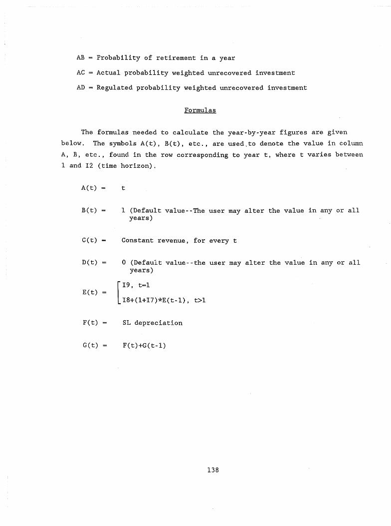
AB Probability of retirement in a year
AC Actual probability weighted unrecovered investment
AD Regulated probability weighted unrecovered investment
Formulas
The formulas needed to calculate the year-by-year figures are given
below. The symbols A(t), B(t), etc., are used,to denote the value in column
A, B, etc., found in the row corresponding to year t, where t varies between
1 and 12 (time horizon).
A(t)
B(t)
C(t)
D(t)
E(t)
F(t)
G(t)
t
1 (Default value--The user may alter the value in any or all years)
Constant revenue, for every t
o (Default value--the user may alter the value in any or all years)
[
19, t=l
18+(I+I7)*E(t-l), t>l
SL depreciation
F(t)+G(t-l)
138
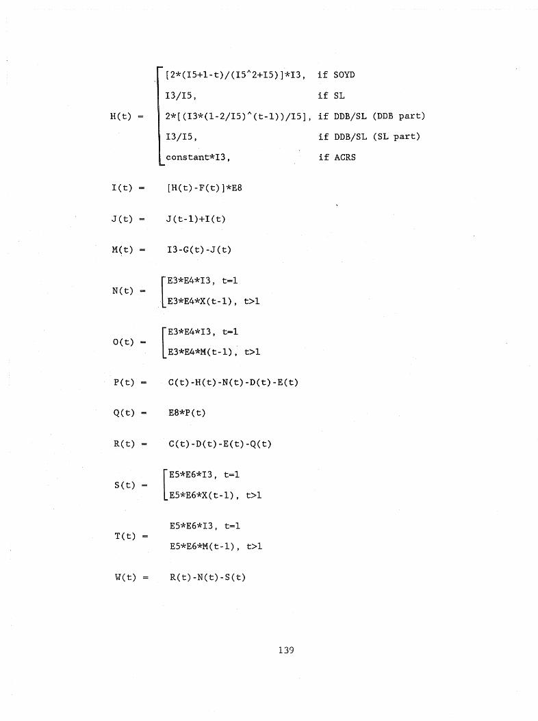
[2*(15+1-t)/(IS A2+15)]*13, if SOYD
13/15, if SL
H(t) 2*[(13*(1-2/15)A(t-l»/15], if DDB/SL (DDB part)
13/15, if DDB/SL (SL part)
constant*13, if ACRS
l(t) [H(t)-F(t)]*E8
J (t) J(t-l)+I(t)
M(t) 13-G(t)-J(t)
[E3*E4*I3 t-l N(t)
. E3*E4*X(~-1)' t>l
[
E3*E4*13 t=l O(t) = '
E3*E4*M(t-l), t>l
P(t) = C(t)-H(t)-N(t)-D(t)-E(t)
Q(t) = E8*P(t)
R(t) C(t)-D(t)-E(t)-Q(t)
[
E5*E6*13 t=l S(t) ,
E5*E6*X(t-l), t>l
E5*E6*13, t=l T(t)
E5*E6*M(t-l), t>l
W(t) R(t)-N(t)-S(t)
139
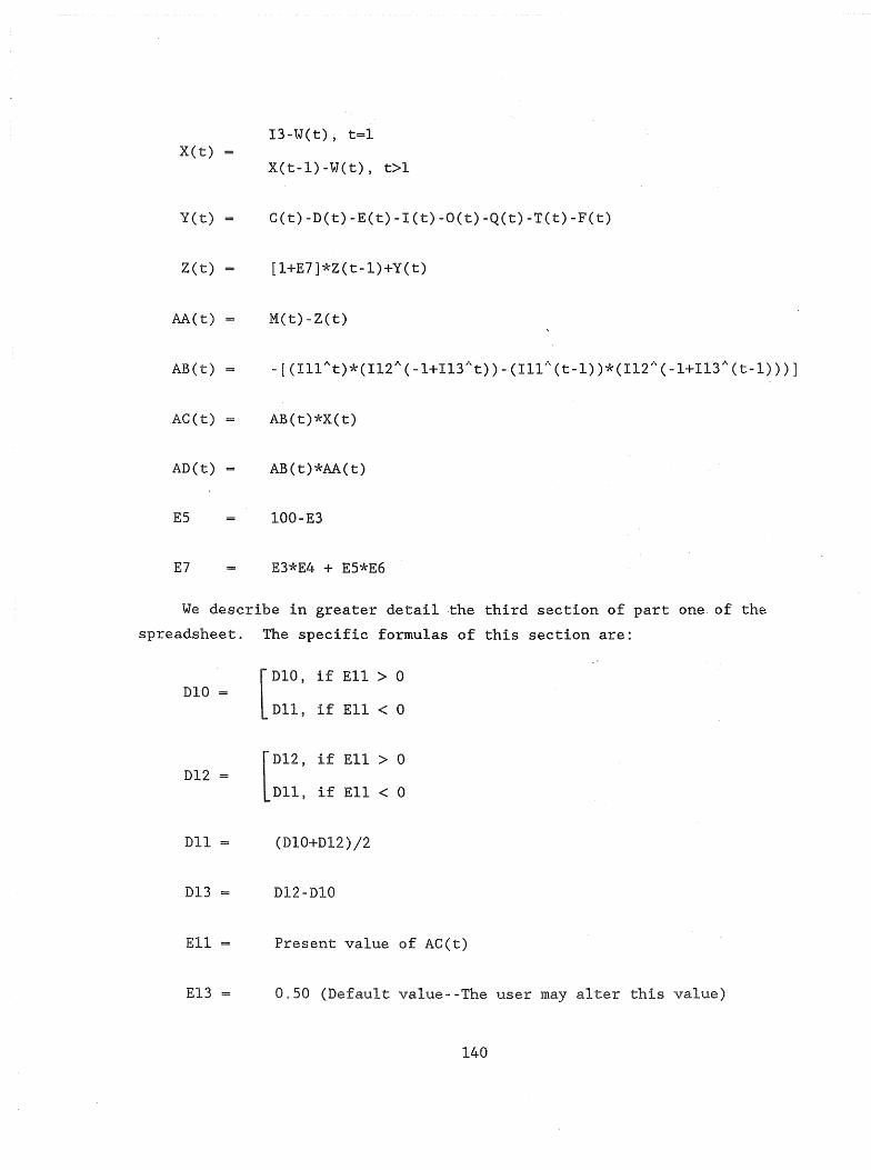
X(t) I3-W(t), t=l
X(t-l)-W(t), t>l
yet) G(t)-D(t)-E(t)-I(t)-O(t)-Q(t)-T(t)-F(t)
Z(t) [1+E7)*Z(t-l)+Y(t)
AA(t) M(t)-Z(t)
AB(t)
AG(t) AB(t)*X(t)
AD(t) AB(t)*AA(t)
ES 100-E3
E7 E3*E4 + ES*E6
We describe in greater detail the third section of part one of the
spreadsheet. The specific formulas of this section are:
[
D10, if Ell > 0 D10
Dll, if Ell < 0
[
D12, if Ell> 0 D12
Dll, if Ell < 0
Dll (D10+D12)/2
D13 D12-D10
Ell Present value of AG(t)
E13 0.50 (Default value--The user may alter this value)
140
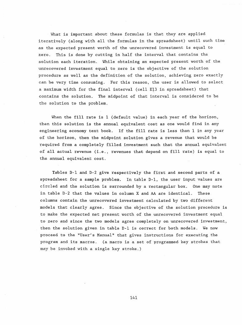
What is important about these formulas is that they are applied
iteratively (along with all the formulas in the spreadsheet) until such time
as the expected present worth of the unrecovered investment is equal to
zero. This is done by cutting in half the interval that contains the
solution each iteration. While obtaining an expected present worth of the
unrecovered investment equal to zero is the objective of the solution
procedure as well as the definition of the solution, achieving zero exactly
can be very time consuming. For this reason, the user is allowed to select
a maximum width for the final interval (cell Et3 in spreadsheet) that
contains the solution. The midpoint of that interval is considered to be
the solution to the problem.
When the fill rate is I (default value) in each year of the horizon,
then this solution is the annual equivalent cost as one would find in any
engineering economy text book. If the fill rate is less than I in any year
of the horizon, then the midpoint solution gives a revenue that would be
required from a completely filled investment such that the annual equivalent
of all actual revenue (i.e., revenues that depend on fill rate) is equal to
the annual equivalent cost.
Tables D-I and D-2 give respectively the first and second parts of a
spreadsheet for a sample problem. In table D-I, the user input values are
circled and the solution is surrounded by a rectangular box. One may note
in table D-2 that the values in column X and AA are identical. These
columns contain the unrecovered investment calculated by two different
models that clearly agree. Since the objective of the solution procedure is
to make the expected net present worth of the unrecovered investment equal
to zero and since the two models agree completely on unrecovered investment,
then the solution given in table D-1 is correct for both models. We now
proceed to the "User's Manual" that gives instructions for executing the
program and its macros. (a macro is a set of programmed key strokes that
may be invoked with a single key stroke.)
141
TABLE D-1
PART ONE OF A SAMPLE PROBLEM
Capital Structure:
Percentage composed of debt = (40.0%) Average interest rate on debt ~
Percent composed of equity 60.0%
Avg rate of return on equity =(20.0~
Composite Cost of Capital 15.6%
Composite Income Tax Rate = <:46.0%)
Solution:
Lower Bound: $379.00 E NPV UI:
Mid Point: $379.16 1($0.3169) t Upper Bound: $379.32 Req'd Width:
Width: $ 0.318487 $0.500000
142
Other Information: Horizon
Initial amount invested
Regulatory book life
Tax life
Tax depreciation method
O&M growth rate
O&M gradient change
O&M initial cost
(SOyr0 @j)
= <:$10.00)
= ($50.0?)
Gompertz-Makeham parameters:
s = 0.99
g 0.955
c = 1.4
TABLE D-2
PART TWO OF A SAMPLE PROBLEM
FIlL SPECIAL O&M BCX]{ Aa:, EO:]( TAX. DEFERRED .AIr.; TAX. \'FAR RATE REVENUES EXPENSES CXlSTS DEP DEP DE? TAXES DE.FERRALS YEAR A B C D E F G H I J K
1 1 $379.16 $0.00 $ SO.OO $125.00 $ 125.00 $333.33 $ 95.83 $ 95.83 1 2 1 379.16 0.00 61.SO 125.00 250.00 266.67 65.17 161.00 2 3 1 379.16 0.00 73.35 125.00 375.00 200.00 34.50 195.50 3 4 1 379.16 0.00 85.55 125.00 500.00 133.33 3.83 199.33 l.
5 1 379.16 0.00 98.11 125.00 625.00 66.67 (26.83) 172. SO 5 6 1 379.16 0.00 111.06 125.00 750.00 0.00 (57. SO) 115.00 6 7 1 379.16 0.00 124.39 125.00 875.00 0.00 (57.SO) 57.50 7 8 1 379.16 0.00 138.12 125.00 1000.00 0.00 (57.50) 0.00 8 9 1 379.16 0.00 152.26 0.00 1000.00 0.00 0.00 0.00 9
PATE Th'TEREST CN DEBT TAXABlE INIME AFTER TAX ErPI1Y lNCI:ME 'YEAR. BASE (ACIUAL) (AJ.l.(JJfj) ) INCX:ME TAX. CASH FlfJ.J (ACIUAL) (A.I.l..CWED ) YEAR L M N 0 p Q R S T U
1 $779.17 $ 36.00 $ 36.00 ($ 40.17) ($ 18.48) $347.64 $120.00 $120.00 1 2 589.00 29.10 28.05 (21.89) 10.07 307.59 97.00 93.50 2 3 429.50 22.57 21.20 83.25 38.29 267.52 75.23 70.68 3 4 300.67 16.46 15.46 143.82 66.16 227.46 54.86 Sl.54 4 5 202.50 10.84 10.82 203.54- 93.63 187.42 36.12 36.08 5 6 135.00 5.78 7.29 262.32 120.67 147.43 19.27 24.30 6 7 67.50 1.37 4.86 253.40 116.56 138.21 4.58 16.20 7 8 0.00 (3.39) 2.43 244.43 112.44 128.60 (11.29) 8.10 8 9 0.00 (8.55) 0.00 235.44 108.30 118.59 (28.49) 0.00 9
~ PROBABTI.l'l'Y l'ROBABTI..I1Y 'WEIQIT'ED CAPITAL l1NREDJVERED Rm.llATCRY ACt:; FW OF Rro!JIATED OF RETIPJ!'MElI.'T UNREC.lJIJERD JNVES".!MFl.'T
YEAR a:NSlMPTICN INVE'S'IMTh'T SI.RPIlJS st:RPllJS INVES1MENI' IN mE YEAR (ACIUAL) (REX;(JIATED ) WAR V W X Y Z AA N!i u::. p.J) A£
1 $191.64 $808.36 ($ 29.19) ($ 29.19) $808.36 0.03 $ 22 69 $ 22.69 1 2 181.48 626.88 (4.13) (37.88) 626.88 0.03 21.45 21.45 2 3 169.73 457.15 16.14 (27.65) 457.15 0.04 19.33 19.33 3 4 156.14 301.01 31.62 (0.34) 301.01 0.05 15.85 15.85 l.f
5 140.46 160.55 42.35 41.95 160.55 0.07 10.50 10.50 5 6 122.39 38.16 48.34 96.84 38.16 O.OS 3.07 3.07 6 7 132.26 (94.10) 49.65 161.60 (94.10) 0.10 (9.06) (9.06) 7 8 143.28 (237.38) SO.57 237.38 (237.38) 0.11 (26.34) (26.34) 8 9 155.62 (393.00) 118.59 393.00 (393.00) 0.49 (192.47) (192.47) 9
143
User's Manual
This user's manual begins by giving the step-by-step procedures that
one would follo'VT in order to produce the results displayed in tables D-1 and
D-2. All other problems may be solved with identical steps; only the data
supplied at each step will change from problem to problem. In addition, a
number of other macros are available to automatically accomplish other
tasks, and data items in individual cells may be changed and the problem
resolved to accomplish "what if" analyses. These other macros are described
after the sample problem exercise.
Sample Problem Exercise
After the Lotus 1-2-3 system has been loaded, the 'following steps
should be followed within the Lotus environment:
1) To load and execute (retrieve) the CAPCOST model spreadsheet, type
the following: /FRCAPCOST then press ENTER (carriage return).
(Note: Capital letters are not required)
2) To solve a problem, one must input data using a set-up routine.
To execute the set-up macro, press the (ALT) key and S at the same
time. Now the program is ready for the user's input. The
following message is displayed at the top of the screen:
- ENTER % COMPOSED OF DEBT (0,1):
The (0,1) means that it expects the input to be a number between ° and
1. For example, in our problem, the percentage of the capital structure
that is composed of debt is 40%. Thus, our input would be 0.40.
144

After each input, press ENTER. At this time the macro will
automatically skip to the next cell that requires an input value.
Altogether, the macro will automatically guide the user through the four
sets of input data that are required.
Set 1: (Capital Structure and Income Tax Information)
The messages will read:
- ENTER % COMPOSED OF DEBT (0,1): for the example, user enters 0.40 - ENTER AVG % RATE ON DEBT (0,1): for the example, user enters 0.09 - ENTER ROR ON EQUITY (0,1): for the example, user enters 0.20 - ENTER INCOME TAX RATE (0,1): for the example, user enters 0.46
Set 2: (Time information)
The messages will read:
- ENTER TIME HORIZON: for the example, user enters 9 - ENTER AMOUNT INVESTED: for the example, user enters 1000 - ENTER REGULATORY BOOK LIFE: for the example, user enters 8 - ENTER TAX LIFE: for the example, user enters 5
As soon as the tax life is entered, the cell labeled "tax depreciation
method" is highlighted and instead of a message appearing on the command
line of the screen, the following menu will appear:
SOYD SL DDB/SL ACRS
The user must choose the preferred method of tax depreciation.
Use left and right arrows to select the choice and then press Enter
(SOYD is selected in this sample problem),
Set 3: (Operations and Maintenance Information)
The messages will read:
- ENTER O&M GROWTH RATE (0,1): for the example, user enters 0.03 - ENTER O&M GRADIENT CHANGE: for the example, user enters 10 - ENTER O&M INITIAL COST: for the example, user enters 50
Set 4: (Survival Curve Parameters)
The messages will read:
- ENTER THE s VALUE: for the example, user enters 0.99 - ENTER THE g VALUE: for ilie example, user enters 0.955 - ENTER THE c VALUE: for the example, user enters 1.4
145

The program now starts executing a completely automatic sequence of
steps to find a solution to the problem. It takes between 40 and 60
seconds, on the average, to run. It will beep three times when it is done.
The solution of this program consists of the revenue (column C in the
spreadsheet) that will make the expected net present worth of unrecovered
investment (cell Ell in the spreadsheet) equal to zero. This process is
done by running an iteration program that searches for the solution that
satisfies that objective. This iteration progFam is automatically executed
at the end of the set-up macro.
Additional Activities and Macros
Suppose that the user needs to change some input cell such as time
horizon, tax depreciation method, etc., after slhe has already run the set
up program. In such a case, the user need not run the 'set-up program again
but may follow one of the following activities depending on what changes
s/he has to make.
Making a Change in Time Horizon
If the user wishes to run the program again, but with a new time
horizon and keeping all other inputs as before, press (ALT) and H at the
same time. The following message will appear: - ENTER NEW TIME HORIZON:
Input your choice, then press ENTER. The program will then rerun the
solution procedure with the new time horizon.
Making a Change in Tax Depreciation Method
If it is desired to change the tax depreciation method, (ALT) and D
should be pressed at the same time. The menu described earlier will appear
again on your screen. Select your choice, then press ENTER. The program
will then rerun the solution procedure with the new tax depreciation method.
146
Making a Change in Other Input Data
If it is desired to change any input other than time horizon or tax
depreciation method, simply go to the input cell you desire to change and
type the new number and press ENTER. A CALC sign will appear on the lower
right corner of the screen. This means that the user should press the key
function F9 to recalculate the spreadsheet. In addition, press (ALT) and I
at the same time to activate the iteration program. The program will then
rerun the solution procedure with the changes that are made. (Note: The
user may change mpre than one input cell before pressing (ALT) and I).
Making a Change in Fill Rate or Special Expenses
If it is desired to change the fill rate or the special expenses in any
year, simply go to the desired cell in columns B or D, respectively, which
corresponds to the specific year the user wants to change and type the new
number and press ENTER. A CALC sign will appear on the lower right corner
of the screen. This means that the user should press the key function F9 to
recalculate the spreadsheet. In addition, press (ALT) and I at the same
time to activate the iteration program. The program will then rerun the
solution procedure with the changes that are made.
Making a Change in Probability of Retirement
If the user decides to use a different survival curve, simply go to the
AB column and manually input the new probabilities in each year. The user
should make sure that the sum of all the probabilities in the specified time
horizon is 1. A CALC sign will appear on the lower right corner of the
screen. This means that the user needs to press the key function F9 to
recalculate the spreadsheet. In addition, press (ALT) and 1 at the same
time to activate the iteration program. The program will then rerun the
solution procedure with the new retirement probabilities.
147
To a of the spreadsheet, press (ALT) and P at the same
time. Make sure that the is on and that the paper is at the right
position on 'the first line of the page.
If it is desired to view some graphs on the screen, press (ALT) and G
at the sarne time. A menu will show up on the top line of the screen with
different
RB-T: RA~E BASE VS TIME
2) SUR-T: REGULATORY SURPLUS VS TIME
3) U . INV .. T: UNRECOVERED INVESTMENT VS TIME
SUR~·U, INV: REGULATORY SURPLUS VS UNRECOVERED INVESTMENT
5) DEP-T: DEPRECIATION VS TIME (both book and tax)
6) ATCF-T: AFTER TAX CASH FLOW VS TIME
) POR-T: PROBABILITY OF RETIREMENT VS TIME
8 : END GRAPH SESSION
Use and left arrows to select your option and press ENTER. To go
back the menu, press ENTER To get out of the menu, choose the
If it is desired to
is
, press (ALT) and Q at the same time. The
saved under the name puca and not under the
name CAPCOST, CAPCOST should always be an empty spreadsheet. It
should. used when ired to solve a new problem.
148

(ALT) S - --> (ALT) H - -->
(ALT) D - --> (ALT) I --->
(ALT) P - -->
(ALT) G - -->
(ALT) Q - -->
Summary Sheet
Input data and run solution procedure.
Change time horizon and run program again.
Change tax depreciation method and run program again.
Run solution procedure.
Print output on printer. Make sure printer is on, and
the paper is at the right position.
View graphs on screen.
Save worksheet under PUCO name and exit Lotus.
* The (ALT) I (iteration program) is automatically called when the (ALT)
S, the (ALT) H, or the (ALT) D are executed; no need to run (ALT) I if you
are running (ALT) S, (ALT) H, or (ALT) D.
* Never save the worksheet under CAPCOST name. CAPCOST is retrieved only
when solving a new problem and it should always start as an empty worksheet.
149