Motivations for Capital Controls and Their Effectiveness · iii . Abstract . We assess the...

Working Paper/Document de travail 2015-5

Motivations for Capital Controls and Their Effectiveness

by Radhika Pandey, Gurnain K. Pasricha, Ila Patnaik and Ajay Shah

2

Bank of Canada Working Paper 2015-5

February 2015

Motivations for Capital Controls and Their Effectiveness

by

Radhika Pandey,1 Gurnain K. Pasricha,2 Ila Patnaik1 and Ajay Shah1

1Macro/Finance Group National Institute of Public Finance and Policy

New Delhi, India 110067 [email protected] [email protected] [email protected]

2International Economic Analysis Department

Bank of Canada Ottawa, Ontario, Canada K1A 0G9

[email protected]

Bank of Canada working papers are theoretical or empirical works-in-progress on subjects in economics and finance. The views expressed in this paper are those of the authors.

No responsibility for them should be attributed to the National Institute of Public Finance and Policy or the Bank of Canada.

ISSN 1701-9397 © 2015 Bank of Canada

ii

Acknowledgements

We thank Vikram Bahure, Apoorva Gupta and Shekhar Hari Kumar for excellent research assistance. We also thank Rose Cunningham, Michael Ehrmann, Atish Ghosh, seminar participants at the Bank of Canada, European Central Bank, University of Southern California, Canadian Economic Association meetings and research meetings of the National Institute of Public Finance and Policy for useful comments.

iii

Abstract

We assess the motivations for changing capital controls and their effectiveness in India, a country with extensive and long-standing controls. We focus on the controls on foreign borrowing that can, in principle, be motivated by macroprudential concerns. We construct a fine-grained data set on capital control actions on foreign borrowing in India. Using event study methodology, we assess the factors that influence these capital control actions, the main factor being the exchange rate. Capital controls are tightened after appreciation, and eased after depreciation, of the exchange rate. Macroprudential concerns, measured by variables that capture systemic risk buildups, do not seem to be a factor shaping the use of capital controls. To assess the impact of controls, we use both event study and propensity score matching methodologies. Event study methodology suggests no impact of capital controls on most variables evaluated, but reveals limited evidence that capital controls relieve currency pressures in the short term. However, even this limited evidence disappears once selection bias is controlled for.

JEL classification: F32, G15, G18 Bank classification: International topics; Financial stability; Exchange rate regimes; Financial system regulation and policies

Résumé

Les auteurs examinent les raisons pour lesquelles des changements sont apportés au régime de contrôle des mouvements de capitaux en Inde (pays où, de longue date, ces contrôles occupent une place importante), ainsi que l’efficacité de ces modifications. Plus spécifiquement, l’étude porte sur les restrictions touchant les emprunts à l’étranger qui peuvent, en principe, être motivées par des préoccupations d’ordre macroprudentiel. Les auteurs constituent pour ce faire un ensemble très complet de données. Au moyen de l’approche événementielle, ils étudient les facteurs qui influencent les modifications décidées par les autorités, le principal d’entre eux étant le taux de change. Le contrôle des mouvements de capitaux est resserré en cas d’appréciation de la monnaie et assoupli en cas de dépréciation. Les considérations macroprudentielles, évaluées à l’aide de variables rendant compte de l’intensification du risque systémique, ne semblent pas être un facteur déterminant en ce qui concerne la décision de resserrer ou d’assouplir les règles. Pour évaluer l’incidence du contrôle des capitaux, les auteurs emploient l’approche événementielle ainsi que des méthodes d’appariement par score de propension. La première approche donne à penser que le contrôle des capitaux n’a pas d’effet sur la plupart des variables à l’étude, mais qu’il pourrait atténuer les pressions exercées sur la monnaie à court terme. Cependant, une fois le biais de sélection pris en compte, même cette incidence ténue disparaît.

Classification JEL : F32, G15, G18 Classification de la Banque : Questions internationales; Stabilité financière; Régimes de taux de change; Réglementation et politiques relatives au système financier

iv

Non-Technical Summary

The volatility of capital flows during and after the global financial crisis has reopened the debate on the place of capital controls in the policy toolkit of emerging-market economies (EMEs). The international policy debate on capital controls stems from the fact that while restrictions on capital flows can potentially reduce volatile inflows in the country that is imposing them, these controls can have global implications, going beyond the economy in which they are imposed. There are two main objectives that capital control policies could pursue. The first is exchange rate management. Capital controls have been held out as a mechanism for avoiding the excessive exchange rate appreciation associated with surges in net capital inflows. A second possible use of capital controls is as a tool for macroprudential policy, i.e., systemic risk mitigation. An extensive literature has shown that, for EMEs, excessive foreign currency borrowing can lead to future financial crashes, and capital controls can be used to limit this borrowing. In this paper, we construct a precise vocabulary for classifying all capital control actions (CCAs) on foreign borrowing for India and compile a definitive database about these CCAs for the period from January 2004 to September 2013. Using this data set, we address two questions: (i) Under what circumstances do EME policy-makers use capital controls—when exchange rate pressures or systemic risk concerns are predominant? (ii) What impact do different capital controls have? Our focus on India is guided by the literature, which has suggested that once a country achieves an open capital account, episodic introduction of controls is not useful. Hence, if capital controls are to be used as a tool for policy, this has to be done in the context of a comprehensive administrative system for capital controls, where the government has the ability to interfere in all cross-border transactions. India is one of only two major EMEs that have a comprehensive administrative system for capital controls (the other is China). We focus only on controls on foreign borrowing, since these could, in theory, be particularly useful as a tool for macroprudential policy. Our results on the first question suggest that the main factor motivating changes in capital controls seems to have been the exchange rate. Capital controls were tightened after appreciations and eased after depreciations. Measures of systemic risk do not seem to be a factor shaping the use of capital controls. We explore the impact of these actions using event studies. There is a strong selection process at work: CCAs are likely to take place under certain circumstances. We therefore draw on recent developments in propensity score matching to match the date on which a CCA was applied with a similar date with no CCA. This permits causal identification of the impact of the CCA. Our results show no impact of the CCAs in any dimension evaluated. We also analyze several sub-categories of controls to determine whether certain kinds of restrictions would be more effective than others, but find no effect in all subcategories studied.

1 Introduction

The global financial crisis has re-opened the debate on the place of capitalcontrols in the policy toolkit of emerging-market economies (EMEs). Thevolatility of capital flows during and after the global financial crisis, and theuse of capital controls in major EMEs, particularly in Brazil, spawned a vig-orous debate among policy-makers on the legitimacy and usefulness of capitalcontrols. The international policy debate on capital controls stems from thefact that while restrictions on capital flows can potentially stem volatile in-flows in the country that is imposing them, these controls can have globalimplications, going beyond the economy in which they are imposed. Theycan distort the global allocation of capital by diverting inflows to economiesthat allow freer movement of capital. They can also be used as a tool in acurrency war, to reduce appreciation pressures. The International MonetaryFund (IMF) has shifted its position and now suggests that these controlsare a legitimate tool, and may be imposed when a country faces a surge innet capital inflows, even after taking into account multilateral considerations(IMF, 2012).

What goals could capital controls pursue? The first dimension lies in macroe-conomic policy. Capital controls have been held out as a mechanism foravoiding overheating of the economy and excessive exchange rate appreci-ation associated with surges in net capital inflows (Pradhan et al., 2011).Others have argued that while capital controls should not be used as a toolfor macroeconomic policy, they can be useful for macroprudential policy, i.e.,systemic risk mitigation. There are two oft-cited examples of cases wherecapital controls could be useful from a macroprudential perspective. First,when excessive foreign inflows risk creating domestic imbalances that cannotbe directly addressed through domestic prudential regulation (for example,loan-to-value ratios or capital buffers at financial institutions), since the flowsare not directly intermediated through the domestic financial system. In thiscase, proponents argue that controls on cross-border transactions may beuseful (Ostry et al., 2012).

A second instance where, in theory, capital controls may be useful from amacroprudential perspective relates to foreign (and/or foreign currency) bor-rowing in EMEs. An extensive literature has shown that, for EMEs, excessiveforeign currency borrowing can generate sub-optimal outcomes from a sys-temic risk perspective (Goldstein and Turner, 2004; Eichengreen et al., 2007).Given the evidence linking external debt, especially in foreign currencies, tofinancial fragility, capital controls (particularly on foreign borrowing) could,

2

in theory, be justified as a tool for macroprudential management. Specifically,these controls could allow the authorities to influence the level of short-termforeign currency borrowing, high levels of which have been associated withpast EME crises.

The IMF staff position (Ostry et al., 2010) is that capital controls can legit-imately be used in the pursuit of both macroprudential and macroeconomicmanagement, as measures of the last resort. While the IMF has held out thispossibility, a lot remains to be done towards constructing a full strategy thatwould constitute the “best practices” for capital control regulations. Theoperation of a complex system of capital controls is like any other complexintervention by the government: it is vulnerable to problems of political econ-omy with lobbying by special interest groups. Establishing sound governancein the field of capital controls would be akin to establishing sound governancein any other area: the regulators responsible would seek to demonstrate thata minimal intervention is being undertaken in response to an identifiablemarket failure.1

A regulatory framework for capital controls that conforms to best practiceswould have four elements: (i) precise definitions of proposed interventions;(ii) proposed rules governing conditions under which these precise actionsshould be taken; (iii) demonstration of effectiveness in achieving desired out-comes; and (iv) demonstration that the costs are outweighed by the benefits.To build this regulatory framework, policy-makers would draw on the sig-nificant literature that addresses the following four questions: (i) What arecapital controls? (ii) Under what circumstances do EME policy-makers usecapital controls? (iii) What impact do different capital controls have? and(iv) Do the benefits outweigh the costs?

In this paper, we address the first three of the four questions. We constructa precise vocabulary for classifying all capital control actions (CCAs) onforeign borrowing for India and compile a definitive database about theseCCAs. We obtain evidence about the conditions under which policy-makershave used CCAs, distinguishing carefully between exchange rate and macro-prudential objectives. Finally, we obtain evidence about the consequences ofthese actions.

Our focus on India is guided by the literature on capital controls of the1980s and 1990s, and recent work such as Klein (2012). This literature

1For more on sound regulatory policy, see, for example, OECD (2012), which rec-ommends that governments adopt a regulatory impact assessment, which would “clearlyidentify policy goals, and evaluate if regulation is necessary and how it can be most effectiveand efficient in achieving those goals.”

3

has suggested that once a country achieves an open capital account, episodicintroduction of controls is not useful. Hence, if capital controls are to be usedas a tool for policy, this has to be done in the context of a comprehensiveadministrative system for capital controls, where the government has theability to interfere in all cross-border transactions.

At present, only two large economies have a comprehensive administrativesystem of capital controls: China and India. Every kind of cross-bordertransaction is controlled and de jure capital account integration, as mea-sured by the Chinn and Ito (2008) measure, is very low. The empiricalevidence drawn from these countries may provide insights on the followingfour questions: What kinds of interventions have been used? When havethey been used? Have they yielded results? Do the benefits outweigh thecosts?

The measurement of CCAs is a challenging task. It is extremely difficultto capture the various kinds of capital controls in a simple measure thatcan be used for empirical analysis. The mainstream cross-country literaturehas relied on crude indices of capital controls, for example, annual readingsin the Chinn-Ito measure. A novel strategy adopted in the recent literatureconsists of closely examining actions, in contrast to levels studied in the olderliterature. Studying individual CCAs allows us to observe their precise datesand to precisely classify the nature of the interventions.

Forbes et al. (2013) construct a database of CCAs drawing mainly on datafrom the IMF Annual Report on Exchange Arrangements and ExchangeRestrictions (AREAER) for 60 countries, for the 2009-11 period. While thisconstitutes better measurement of capital controls, the IMF AREAER dataare a coarse measure of CCAs.

A key innovation toward better measurement of CCAs was the data set con-structed by Pasricha (2012), which utilizes AREAER, regulators’ websitesand news sources to identify CCAs in 22 emerging economies. It also countsactions separately by asset class (for example, foreign borrowing, foreign di-rect investment (FDI), portfolio investments, etc.) and by type (quantitative,price-based, etc.). This reveals a much larger number of CCAs when com-pared with events reported in the AREAER, and permits better classificationof actions, which can then reveal their consequences.

In this paper, we take the next step forward: measuring CCAs with a carefulclassification of the various aspects of regulations (e.g., controls on minimummaturity of loans, controls on eligible borrowers, interest rate ceilings, etc.).To ensure comprehensive coverage and accurate interpretation of the regula-

4

tory actions (including whether the action represented an easing or tighteningof controls), we used a legal team that read every legal instrument associ-ated with the CCA. On average, our lawyers spent three man-hours per legalinstrument, and constructed a fine-grained data set about CCAs on one as-set class: foreign borrowing. Our focus is on foreign borrowing, since it iscritically connected with questions of systemic risk.

Our data set covers the period from January 2004 to September 2013 andcontains 75 CCAs. It permits us to explore two other main questions inthe field. The first finding concerns the circumstances under which EMEpolicy-makers use capital controls on foreign borrowing. The main factorthat seems to be at work is the exchange rate. Capital controls are tightenedafter appreciations and eased after depreciations. Measures of systemic riskdo not seem to be a factor shaping the use of capital controls.

What was the impact of these actions? We explore the impact of these actionsusing event studies. There is a strong selection process at work: CCAs arelikely to take place when faced with certain circumstances. Hence, we drawon recent developments in propensity score matching, to match the date onwhich a CCA was applied against a similar date with no CCA. This permitscausal identification of the impact of the CCA. Our results show no impact ofthe CCAs in any dimension evaluated. We also analyze some sub-categoriesof controls to determine whether certain kinds of restrictions would be moreeffective than others, but find no effect in all subsets studied.

The remainder of this paper is organized as follows. Section 2 reviews theexisting literature on the four major questions and places our contributionsin context. Section 3 describes recent developments in the measurement ofCCAs. Section 4 describes the Indian system of capital controls, with anemphasis on capital controls against foreign borrowing, and documents theconstruction of the novel data set about Indian CCAs on foreign borrowing.Section 5 explains the data and methodologies used in the paper. Section6 identifies the factors that shape the use of CCAs. Section 7 measures theimpact of these actions. Section 8 concludes.

2 Research questions in the field of capital

controls

In a well-functioning system, the power of the state is located within a frame-work of objectives, minimal coercive power and accountability mechanisms.

5

If capital controls were to become a mainstream tool that is used in a well-structured regulatory process and conforms to the best practices in regulatorypolicy, certain conditions would need to be fulfilled. A precise statement ofthe proposed intervention would be required, along with specification of theconditions under which the restriction would kick in. In order to aid thedevelopment of best practices in capital controls policy, the literature needsto address four questions, discussed below.

2.1 What are capital controls?

A very wide array of impediments to cross-border transactions are all cov-ered by the broad term “capital controls”. For capital controls to establishthemselves as part of an optimal policy toolkit, it is important to arrive atprecisely articulated interventions and a shared vocabulary, through whichthese interventions can be discussed, enacted and evaluated.

The literature on the effectiveness of capital controls has been based on mea-sures of capital controls that are too broad to provide useful guidance toregulators about the impact of specific interventions.2 Emerging economiesuse many different types of regulations on cross-border transactions, rangingfrom quantitative controls (for example, on foreign investment in the securi-ties market), to price-based restrictions (such as the maximum interest ratepayable on foreign borrowings) and approval and reporting requirements.Further, the literature on capital controls in the 1980s and 1990s, and recentwork such as Klein (2012) emphasize that controls introduced episodicallyare not effective. Hence, if capital controls are to be useful in meeting thegoals of economic policy, there needs to be a comprehensive administrativesystem for capital controls, where the government has the ability to interferein all cross-border transactions.

These considerations suggest that in order to provide useful guidelines toregulators, the literature on capital controls needs to specify, categorize andassess the full array of restrictions on cross-border regulations. As mentionedin the introduction, a recent wave of literature has started this process (Pas-richa, 2012; Hutchison et al., 2012; Forbes et al., 2013). We go further in thisdirection by constructing a fine-grained data set of capital control actions(CCAs) that separately classifies every aspect of regulation in India relatedto foreign borrowing.

2See Magud et al. (2011) for a survey. The exceptions are some country specific studies,most of which assess the impact of unremunerated reserve requirements or inflow taxes inLatin American countries.

6

2.2 Under what circumstances do EME policy-makersuse capital controls?

Do EME policy-makers use capital controls to achieve exchange rate objec-tives or to pursue systemic risk objectives? Factually assessing the motiva-tions for past EME CCAs can help inform the debate on capital controls, aswell as the resulting international consensus on the rules of governance fortheir use. One the one hand, if it can be discerned in the data that emergingmarkets have, in fact, been using capital controls to target systemic risk, thisbolsters the legitimacy of the EME case for continued use of these instru-ments. On the other hand, if the data suggest that CCAs have been used forcurrency manipulation, this bolsters the case of those who argue that fur-ther international discussions on the rules of the game are needed to addressmultilateral concerns.

The recent debate has almost entirely focused on what emerging economiesshould do; evidence of what motivates their actions is a nascent area of re-search. Pasricha (2012) uses data on CCAs on a broad range of internationalcapital transactions for 18 EMEs over the period 2004-10 and finds that theuse of CCAs follows trends in net capital inflows — measures to reduce netcapital inflows were at their peak in 2007 and 2010, when net capital inflowsto EMEs were at their peak. Pasricha also finds that the majority of CCAswere not “prudential-type measures,” i.e., they were not directly targeted toaddress a buildup of financial risk. Aizenman and Pasricha (2013) focus ononly CCAs on outflows by residents and find that these were also motivatedby net capital inflow pressures. Fratzscher (2012) uses the measures of de jurelevels of capital controls (Chinn-Ito (2008) and Schindler (2009) indices) toassess macroprudential vs. exchange rate objectives and finds that exchangerate and overheating pressures primarily drove CCAs in a broad sample ofcountries. This paper uses an event study to provide a systematic evaluationof macroprudential vs. macroeconomic objectives using detailed data on atype of instrument — controls on foreign borrowing — that, in principle,would be well-suited to address systemic-risk concerns.

2.3 What impact do different capital controls have?

Empirical evidence about the impact of each type of capital control onmacroeconomic outcomes and vulnerabilities in the financial system wouldprovide us with an understanding of the conditions under which differentkinds of capital controls are appropriate. This understanding can then be

7

translated into optimal rules for financial regulators.

Ostry et al. (2012) find a statistically significant association between financialsector-specific capital controls and lower foreign exchange borrowing. Em-pirical analysis by Ostry et al. (2010) suggests that countries with controlson debt flows fared better during the recent global financial crisis. However,empirical analysis by Blundell-Wignall and Roulet (2013) qualifies these re-sults, finding that while certain kinds of restrictions on inflows (particularlydebt liabilities) were most useful in good times, lower controls on bonds andon FDI inflows were associated with better growth outcomes during the re-cent global financial crisis period. Our data set allows us to capture preciselythe nature of and dates of each of the CCAs, so that their impact on differ-ent macroeconomic and financial variables can be isolated in an event studysetting.

2.4 Do the benefits outweigh the costs?

Cost-benefit analyses allow us to weigh the microeconomic and political econ-omy problems associated with capital controls against the putative gains.Cost-benefit analysis is a key mechanism for improving the quality of workin the regulation-making process and much remains to be done in the areaof capital controls. Such an assessment, however, is also beyond the scope ofthis paper.3

3 Measurement of capital control actions

An assessment of the motivations for and effectiveness of capital controls iscomplicated by the challenges involved in the measurement of capital controlactions (CCAs). It is extremely difficult to capture the various kinds ofcapital controls in a simple measure that can be used for empirical analysis.

3On the cost-assessment side, a wide body of research on capital controls focuses onmicroeconomic distortions from capital controls (Edwards and Ostry, 1992; Edwards, 1999;Forbes, 2005, 2004). On the benefits side, the evidence is mixed regarding the extent towhich capital controls are able to deliver on the objectives of macroeconomic policy. Whilecapital controls seem to be able to change the composition of flows toward more long-termdebt, it is not clear to what extent this represents a mislabelling of flows (Magud et al.,2011; Carvalho and Garcia, 2008). Patnaik and Shah (2012) find that the Indian capitalcontrols are not an effective tool for macroeconomic policy.

8

Figure 1 De jure measures of capital account openness: India

1970 1980 1990 2000 2010

−1.

6−

1.4

−1.

2−

1.0

−0.

8C

hinn

−Ito

Sco

re

(a) Chinn-Ito measure

1996 2000 20040.

850.

900.

951.

00S

chin

dler

Sco

re

Overall scoreInflows ScoreOutflows

(b) Schindler measure

The mainstream cross-country literature has relied on crude indexes of capitalcontrols. Existing measures of de jure capital account openness, such asthe Chinn and Ito (2008)4 and the Schindler (2009) indexes,5 measure thelevel of capital controls using the summary classifications table published bythe IMF in the AREAER.6 While these measures are easily compiled andhelpful in cross-country comparisons, they do not capture the complexityof capital controls, particularly when a complex administrative system ofcapital controls is in place.

As Figure 1 shows, the Chinn and Ito (2008) measure does not detect anychange in India’s level of openness, i.e., no change in capital controls, for theentire time series from 1970 to 2010. The Schindler (2009) measure appearsto do better, by showing at least some variation in the level of openness, butthe observed variation is very minor compared with the changes that havetaken place in the regime between 1995 and 2005 that are better reflectedin the India-specific indexes constructed by other papers (Hutchison et al.,2012; Jadhav, 2003).

4The Chinn-Ito measure ranges from -1.83 to 2.53, with -1.83 being a closed capitalaccount economy and 2.53 being an open economy.

5The Schindler measure ranges from 1 to 0, with 1 being a closed capital accounteconomy and 0 being an open economy.

6The IMF has been reporting on exchange arrangements and restrictions from 1950onward and provides a description of the foreign exchange arrangements, exchange andtrade systems, and capital controls of all IMF member countries. The AREAER hasprovided a summary of capital controls for a wide cross section of countries since 1967.

9

The problem with measures based on the AREAER classification table isthat they detect a move toward capital account openness only when an en-tire sub-category of controls is dismantled. In cases of countries like India,the process of capital account liberalization has gone from complete prohibi-tions to complex bureaucratic procedures. The process has generally movedtoward greater capital account openness, but without dismantling the struc-ture of controls. This allows authorities to retain their ability to reverse pastliberalizations. These complexities are hard to capture in summary measuressuch as those of Chinn and Ito (2008) and Schindler (2009). Another con-straint with these databases is their frequency: they report one value everyyear. This prevents the use of high-frequency data in analyzing the impactof changes in capital controls.

A key innovation of the recent literature is its shift in focus from the levelof capital account openness to individual capital control actions (CCAs).Although it may be hard to quantify the extent of restrictions present ata point in time, it is more feasible to unambiguously identify the date of aCCA, and to place it within a classification system. This permits the analysisof changes in the system of capital controls, using high-frequency data andhigh-quality measurements of each CCA.

This strategy is used by Forbes et al. (2013), which is primarily based on theAREAER, supplemented with news sources. This paper covers 60 countriesfor a short window of time (2009-11). For example, this data set containsseven actions—five easings and two tightenings—for India.

Pasricha (2012) constructs a fine-grained database of CCAs in 22 emergingmarkets for the period 2004-10. This paper also uses data from AREAER,but extends it by obtaining information on similar measures from websites ofcentral banks and other regulators, news sources, and other research papers.To increase comparability among actions, capital control changes announcedon the same date are broken down by the asset classes that they affect (e.g.,portfolio flows, FDI, etc.) and the type of change (quantitative, monitoringor price-based), and each is counted as a separate action. For example,for 2009-11, this data set (extended in Hutchison et al. (2012)) contains 27actions relating to inflow controls for India, out of which 9 relate to foreignborrowing restrictions.

In this paper, we take the next step by constructing a high-quality data set onCCAs. The classification system tracks changes in each aspect of regulationson foreign borrowing. For example, changes in quantitative limits on foreignborrowing are counted independently of changes in permissible end-uses ofthe funds borrowed, even if announced on the same date. This yields a

10

finer classification system for these actions. For example, for capital controlsagainst foreign borrowing only, for 2009-11, this data set contains 14 actions.

4 The setting

4.1 Capital controls in India

Capital controls were introduced in India by the British colonial authoritiesin 1942 as a temporary wartime measure. They gradually evolved into acomprehensive system of restrictions on cross-border capital mobility withthe Foreign Exchange Regulation Act (FERA 1973), which criminalized vi-olations. At the time, current account integration was also highly restricted.The conditions associated with a 1991 IMF program required eliminatingcontrol of the current account and the capital account. The current accounthas become open and FERA was replaced by a new law, the Foreign Ex-change Management Act (FEMA 1999), under which violations of capitalcontrols were no longer criminal offences, but were civil offences.

All capital account transactions are prohibited unless explicitly permitted.The permissions are granted through a set of legal instruments issued by theReserve Bank of India (RBI) and the Ministry of Finance. Restrictions differaccording to the type of investor, the asset class, the recipient of foreigncapital, the intended end-use of the foreign capital, etc.

There are three areas where there are no restrictions on the size of invest-ments: inbound FDI, outbound FDI and foreign investment in the equitymarket. In all other areas, quantitative restrictions are in place, throughwhich the RBI specifies caps on cross-border activities. For example, there isa cap on the aggregate ownership by all foreign investors of rupee-denominateddebt. Similarly, there is a cap on the amount of capital that can be takenout of the country each year by one resident.

There is no unified manual or legal document that shows all the capitalaccount restrictions that are in place. Sinha (2010) is a useful description ofthe capital controls prevalent in 2010.

11

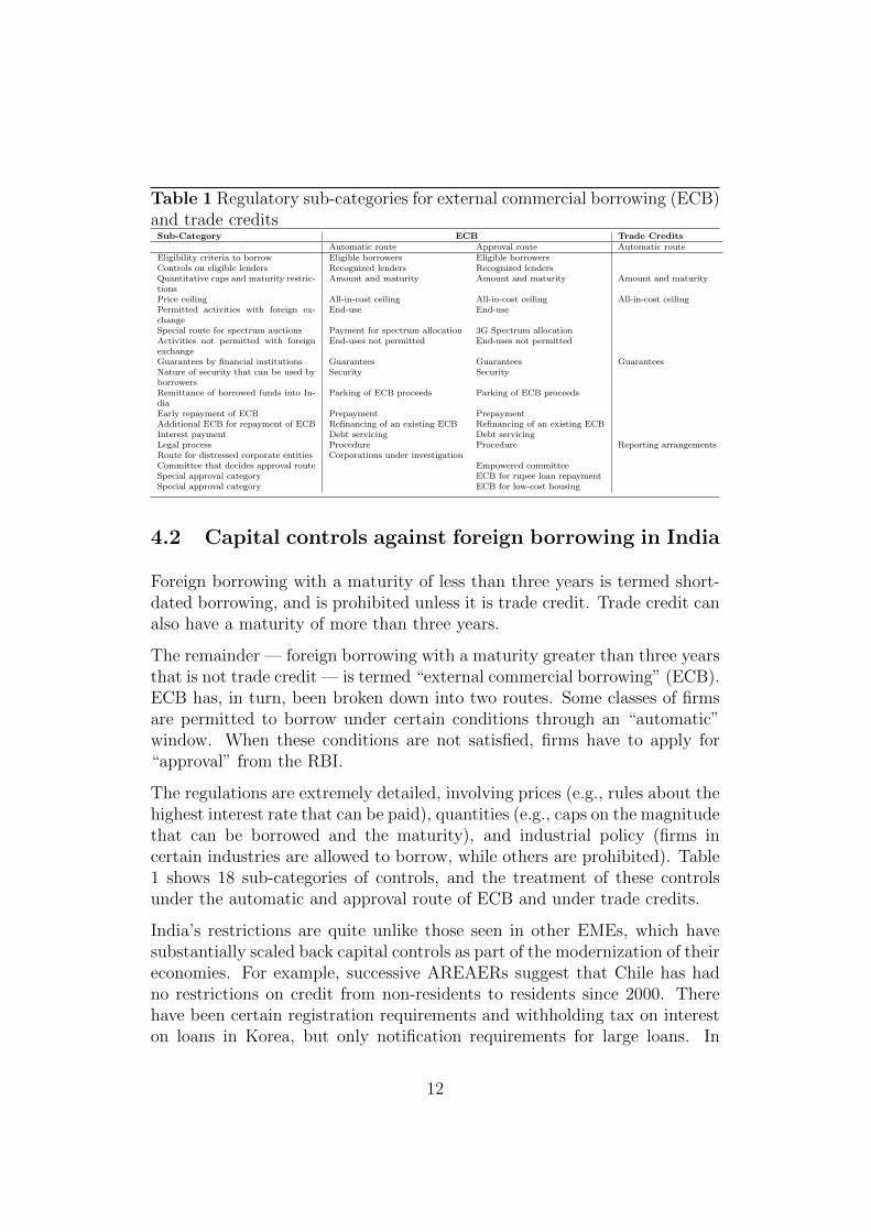
Table 1 Regulatory sub-categories for external commercial borrowing (ECB)and trade creditsSub-Category ECB Trade Credits

Automatic route Approval route Automatic routeEligibility criteria to borrow Eligible borrowers Eligible borrowersControls on eligible lenders Recognized lenders Recognized lendersQuantitative caps and maturity restric-tions

Amount and maturity Amount and maturity Amount and maturity

Price ceiling All-in-cost ceiling All-in-cost ceiling All-in-cost ceilingPermitted activities with foreign ex-change

End-use End-use

Special route for spectrum auctions Payment for spectrum allocation 3G Spectrum allocationActivities not permitted with foreignexchange

End-uses not permitted End-uses not permitted

Guarantees by financial institutions Guarantees Guarantees GuaranteesNature of security that can be used byborrowers

Security Security

Remittance of borrowed funds into In-dia

Parking of ECB proceeds Parking of ECB proceeds

Early repayment of ECB Prepayment PrepaymentAdditional ECB for repayment of ECB Refinancing of an existing ECB Refinancing of an existing ECBInterest payment Debt servicing Debt servicingLegal process Procedure Procedure Reporting arrangementsRoute for distressed corporate entities Corporations under investigationCommittee that decides approval route Empowered committeeSpecial approval category ECB for rupee loan repaymentSpecial approval category ECB for low-cost housing

4.2 Capital controls against foreign borrowing in India

Foreign borrowing with a maturity of less than three years is termed short-dated borrowing, and is prohibited unless it is trade credit. Trade credit canalso have a maturity of more than three years.

The remainder — foreign borrowing with a maturity greater than three yearsthat is not trade credit — is termed “external commercial borrowing” (ECB).ECB has, in turn, been broken down into two routes. Some classes of firmsare permitted to borrow under certain conditions through an “automatic”window. When these conditions are not satisfied, firms have to apply for“approval” from the RBI.

The regulations are extremely detailed, involving prices (e.g., rules about thehighest interest rate that can be paid), quantities (e.g., caps on the magnitudethat can be borrowed and the maturity), and industrial policy (firms incertain industries are allowed to borrow, while others are prohibited). Table1 shows 18 sub-categories of controls, and the treatment of these controlsunder the automatic and approval route of ECB and under trade credits.

India’s restrictions are quite unlike those seen in other EMEs, which havesubstantially scaled back capital controls as part of the modernization of theireconomies. For example, successive AREAERs suggest that Chile has hadno restrictions on credit from non-residents to residents since 2000. Therehave been certain registration requirements and withholding tax on intereston loans in Korea, but only notification requirements for large loans. In

12

Figure 2 Cumulative borrowing through ECB

2004 2006 2008 2010 2012 2014

050

100

150

US

D b

illio

n

AutomaticApproval

Source: RBI monthly statistics

Mexico, there have been no restrictions imposed except for some limits onforeign currency borrowing by banks as a percentage of their net worth and ontheir open foreign exchange positions. In Brazil, there have been no controlsother than, for some time, a transparent tax on short-term borrowing. Andin Turkey, for part of the past decade, there were restrictions in place onforeign currency and foreign currency-linked consumer and mortgage loans.

4.3 Foreign borrowing in India

Figure 2 shows the cumulative borrowing that has taken place under ECB(automatic) and ECB (approval) mechanisms over the past decade. Thestock of borrowing in March 2013 was 5.4 times that of March 2004. Ex-pressed as a proportion to total external debt, this foreign borrowing rosefrom 22.9% in March 2004 to 33.4% in March 2013.

5 Data and methodology

5.1 The Indian CCA data set

The RBI is the manager of the FEMA 1999 and has the authority to frameregulations under the Act. Foreign borrowing is governed by foreign exchange

13

management (FEM) regulations, which constitute the capital controls on for-eign borrowing. Amendments to these regulations must be tabled by the RBI(as notifications) and approved by Parliament in order to be legally enforce-able. However, the changes to capital controls are published by the RBI incirculars (and are usually made effective) before the regulatory amendmentsare passed. The RBI also issues master circulars that act as a compendiumof the notifications/circulars issued in the previous year, without necessarilycovering all the details.

The practical implication for economists of this complex system is that some-one looking at the RBI press releases is likely to miss all the changes incontrols. The legal team helped us understand this three-tier system andassisted us in finding all the relevant instruments issued by the RBI over oursample period, i.e., the notifications/circulars and master circulars. Theyalso helped us cross-verify the information in these different instruments,verify that each circular was indeed backed by a notification (regulatoryamendment), and verify the effective dates of each change. Further, the legalinstruments on capital controls, like the text of other laws and regulations,can be hard for the layman to interpret. For example, for certain actions, itmay be difficult for non-experts to correctly understand whether an actionrepresents an easing or a tightening of controls. The legal team also assistedus in this task. Our thorough scan of legal instruments using lawyers’ ex-pertise gives us confidence that the resulting database is comprehensive andaccurate.

Our database has approximately 100 legal instruments, which represent thefull history of capital controls for ECB between January 2004 to September2013. Even though administrative and procedural changes can have a sub-stantial impact on the ability to undertake transactions, the strategy adoptedwas to focus only on substantive changes.

Our approach is to count as separate changes in all aspects of controls onforeign borrowing (the regulatory sub-categories in Table 1) even if one ormore of these are changed on the same date. Our approach differs from re-lated work in this field. For example, if one RBI circular eases the eligibilitycriteria for firms allowed to borrow abroad and also eases the maturity re-strictions, Pasricha (2012) classifies this as one event. We classify this as twodistinct actions. This allows for the analysis of various classes of CCAs onforeign borrowing.7

For our empirical analysis, we drop the dates of mixed events, i.e., dates on

7See Appendix A for further information on our database.

14

Table 2 Tightening and easing events

Sub-categories Easing TighteningAutomatic eligible borrowers 12 1Automatic amount and maturity 8 0Automatic all-in-cost ceilings 1 1Automatic end use 6 1Automatic end use not allowed 0 1Automatic parking 0 1Automatic prepayment 3 0Approval eligible borrowers 17 0Approval amount and maturity 4 0Approval all-in-cost ceilings 2 2Approval end use 9 0Approval parking 0 1Approval prepayment 1 0Trade credit amount and maturity 2 0Trade credit all-in-cost ceilings 3 0Total 68 8

which easing and tightening changes were simultaneously introduced. Wealso drop those changes on controls in foreign borrowing that overlap withother changes in capital controls. This yields a database of unambiguouschanges in capital controls on foreign borrowing with no contemporary con-founding events in terms of CCAs.

Table 2 shows summary statistics on our CCA database. Of a total of 76events, 68 are easing and eight are tightening. The largest number of changesinvolved the definition of the class of firms that were considered eligible forthe automatic route or the approval route. Since most of the records pertainto easing, for much of the analysis that follows in this paper, we analyzeeasing events only.

Table 3 shows the number of records in the database in each year. Themost events occurred in 2012 and 2013, when many CCAs took place toease controls. However, most tightening events took place in 2007, when netcapital inflows to India were surging.

5.2 Measuring macroeconomic vs. macroprudentialobjectives

We use the CCA database to address two questions. First, are CCAs changedin response to macroeconomic management concerns or macroprudential

15

Table 3 Number of CCAs, by year

Year Easing events Tightening events2003 0 12004 2 02005 6 02006 2 02007 1 62008 8 02009 0 02010 8 12011 6 02012 20 02013 15 0Total 68 8

management concerns? Second, what impact did the CCAs have on macro-economic and financial variables?

In order to address these questions, we need to distinguish between vari-ables that represent macroeconomic management objectives from those thatrepresent macroprudential objectives. A joint report by the Bank for Inter-national Settlements (BIS), Financial Stability Board (FSB) and IMF (BISet al., 2011) carefully makes this distinction. In their analysis, macropru-dential policy is defined by its objective of addressing systemic risks in thefinancial sector to ensure a stable provision of financial services to the realeconomy over time. They also recommend that macroprudential policy not beburdened with additional objectives, for example, exchange rate stability orstability of aggregate demand or the current account. This recommendationreflects the emerging consensus view of the best practices in macropruden-tial policy at advanced-economy central banks (Bank of England, 2009; Nieret al., 2013).8 The view that macroprudential policy be primarily accordedthe objective of systemic risk mitigation allows for the use of capital controlsas one of the tools for achieving this objective. However, under this frame-work, assessing whether capital controls have been used as “macroprudentialtools” would necessitate the assessment of systemic risk buildups around the

8This consensus in advanced-economy and multilateral institutions is in contrast tosome of the recent economics literature (and indeed the views of some EME policy-makers)that continues to view exchange rate stabilization and other macroeconomic managementobjectives as part of the goals of macroprudential policy. For example, Blanchard (2013)suggests an approach where monetary policy, exchange rate intervention, macroprudentialmeasures and capital controls are all used to manage the exchange rate, and this is justifiedin order to prevent large exchange rate changes that are thought to cause disruptions inthe real economy and in financial markets.

16

time that controls were changed.

In this paper, we follow the BIS-FSB-IMF approach and distinguish betweenmacroeconomic objectives (exchange rate pressures) and macroprudential ob-jectives. We use four outcome variables to assess exchange rate objectives:

1. INR/USD returns: This variable is the daily percentage change in thespot exchange rate of the Indian rupee (INR) against the U.S. dollar(USD). 9

2. Frankel-Wei residual: Consider the exchange rate regression in Haldaneand Hall (1991) that gained prominence after it was used in Frankel andWei (1994). An independent currency, such as the Swiss franc (CHF),is chosen as an arbitrary “numeraire,” and the regression model is

d log(

INR

CHF

)= β1+β2d log

(USD

CHF

)+β3d log

(JPY

CHF

)+β4d log

(DEM

CHF

)+ε

The ε of this regression can be interpreted as the India-specific compo-nent of fluctuations in the INR/USD exchange rate.

3. Exchange market pressure (EMP) index: This variable is the Felmanand Patnaik (2013) measure of exchange market pressure expressed interms of per cent change in exchange rate at a monthly frequency. Itmeasures not only how much the exchange rate actually moved, but alsohow much it would have moved had the central bank not intervenedin the foreign exchange market or changed the interest rates. Positive(negative) values indicate a pressure to depreciate (appreciate).

4. Real effective exchange rate (REER): This variable is the trade-weightedaverage of nominal exchange rates adjusted for the relative price dif-ferential between the domestic and foreign countries.

All exchange rate variables are defined such that an increase in value corre-sponds to a depreciation of the Indian rupee, except the REER, in which anincrease corresponds to appreciation.10

To assess macroprudential objectives, we use the following variables:

1. Foreign borrowing (or external commercial borrowing, ECB): This isthe month-over-month growth in foreign borrowing under the auto-matic and approval route.

9The exchange rate against the U.S. dollar is the key rate for the Indian economy. TheRBI intervenes to mitigate volatility in this rate.

10The data sources for all variables are in Appendix B.

17

2. Private bank credit growth: This is the month-over-month percentagegrowth of non-food credit extended by the banking sector. In order toavoid the confounding effects of the highly volatile inflation time-series,credit growth is re-expressed in real terms.

3. Stock price returns: This is the daily percentage change in the S&PCNX Nifty closing prices.

4. Gross capital inflows: This is the quarter-over-quarter growth in grossflows on the financial account of balance of payments.

5. M3 growth: This is the month-over-month growth in the money supply.

5.3 Methodology: Motivations for CCAs

We approach the question of what motivates the use of CCAs in two ways.The first approach involves using both sets of outcome variables (measuringexchange rate and macroprudential objectives) in a logit model explainingeasing of controls.11 If only exchange rate variables are significant and of theright signs, we may infer that the exchange rate motivations are predominant.The logits are done at a weekly frequency and three lags of each of theoutcome variables are used. The weekly frequency puts a constraint on theoutcome variables we may use in the logits. We also provide results for logitsat a monthly frequency.12 The results are unchanged. For the exchangerate objective, we use two specifications: (i) the spot returns, and (ii) thepredicted portion and the residual from the exchange rate regression usedin Frankel and Wei (1994). To proxy concerns about buildup of financialimbalances, we use growth in the money supply (M3) and the stock market(Nifty) returns.

The second approach is an event study that looks for statistically significanttrends in each of the outcome variables in the period leading up to the eventdate, which is the date of the CCA. One the one hand, if the CCAs are usedas a tool for exchange rate policy, then foreign borrowing is restricted whenthere is pressure to appreciate, and vice versa. On the other hand, a macro-prudential regulator would tighten controls on foreign borrowing in responseto evidence of excessive foreign borrowing, excessive currency mismatches orasset price bubbles. The testable hypotheses (expected trends) for each ofour outcome variables are summarized in Table 4.

11There are not enough tightenings in the sample for a robust logit analysis.12The results are not sensitive to the choice of lag. We tried specifications with one to

four lags for weekly specification and up to three lags for monthly specification.

18

The horizon over which we assess the trends in each variable when assessingmotivations for CCAs is, in general, shorter for the exchange rate variablesthan for the systemic risk variables. The administrative infrastructure forthe controls is well established: the RBI has autonomy on foreign exchangemanagement, and it is able to provide notification of changes with immediateeffect via circulars and later issue regulatory amendments that have alreadybeen approved by Parliament. Further, RBI actions on capital controls takeplace quite frequently. Therefore, we think that the appropriate time horizonfor assessing the exchange rate is no more than three months, but potentiallyshorter. The same holds for market-based variables such as stock prices. Forthe other variables, such as bank credit growth, which are slower moving andfor which information is available only with a lag, we evaluate indicators overa longer horizon before the event, up to six months (for foreign borrowing orbank credit growth) or two quarters (gross capital flows).

For the event study, mean adjustment is used in all cases, where the timeseries of (cumulative) percentage changes is de-meaned. Using cumulativechanges rather than actual changes allows us to control for the fact that someof the announcements may be anticipated (Kothari and Warner, 2007).13

Using non-cumulative changes would put too much weight on the behaviourof the series very close to the announcement of the capital control action(CCA).

To test for statistical significance, the bootstrap procedure for event stud-ies described in Davison et al. (1986) is utilized.14 Inference procedures intraditional event studies were based on classical statistics (for example, thet-statistic). However, classical statistics require distributional assumptions,including normality, independence and lack of serial correlation. Further,the asymptotic properties of the test statistics do not apply for small sam-ples. A large literature has shown that bootstrap methods allow more robustinferences for event studies.15 The bootstrap approach avoids imposing dis-tributional assumptions such as normality, and is also robust against serialcorrelation—the latter being particularly relevant in the context of macroe-conomic variables like exchange rate and foreign inflows.

The bootstrap inference strategy that we use is as follows:

1. Suppose there are N events.16 Each event is expressed as a time series

13For all the changes in our sample, the announcement dates were also the effectivedates of the changes.

14The program is described in Patnaik et al. (2013) and Anand et al. (2014).15See Kothari and Warner (2007) and references therein.16Note that the event study is done at the level of events, not weeks or months. This

19

Table 4 Event study for capital controls motivation: Expected trends

Variable Trend prior toExchange rate objective Easing TighteningINR/USD returns Depreciation AppreciationFrankel-Wei residuals Depreciation AppreciationExchange market pressure Depreciation AppreciationREER Depreciation Appreciation

Macroprudential objective Easing TighteningForeign borrowing (ECB) Slowing IncreasingBank credit growth Slowing IncreasingGross inflows Slowing IncreasingStock price growth Slowing Increasing

of cumulative changes (Cnt , n = 1...N) in event time, within the event

window. The overall summary statistic of interest is the C̄t, the averageover the N time series.

2. We do sampling with replacement at the level of the events. Each boot-strap sample is constructed by sampling with replacement, N times,within the data set of N events. For each draw, the Cn

t time seriescorresponding to one event is taken, and N such draws are made. Av-eraging over the N draws, this yields a time series C̄1t, which is onedraw from the distribution of the statistic.

3. This procedure is repeated 1,000 times in order to obtain the full dis-tribution of C̄t. Percentiles of the distribution are shown in the figuresreported later in the paper, giving bootstrap confidence intervals forour estimates.

5.4 Methodology: Effectiveness of CCAs

To study the effectiveness of capital controls we use two methodologies. First,we conduct event studies starting from the event date, i.e., the date of a CCA.The event studies are done separately on both easing and tightening events,for all events included in the sample. Table 5 presents the testable hypotheses(expected trends) with respect to each of the outcome variables under theassumption that capital controls were effective.

For the event studies of the effectiveness of CCAs, the horizon again depends

means that a week in which there is more than one event is included in the sample asmany times as there are events in that week.

20

Table 5 Event study for capital controls effectiveness: Expected trends

Variables Expected impact ofExchange rate objective Easing TighteningINR/USD returns Appreciation DepreciationFrankel-Wei residuals Appreciation DepreciationExchange market pressure Appreciation DepreciationREER Appreciation Depreciation

Macroprudential objective Easing TighteningForeign borrowing (ECB) Increase DecreaseBank credit growth Increase DecreaseGross inflows Increase DecreaseStock prices Increase Decrease

on the variables, and is shorter for higher-frequency variables. For spot ex-change rates, Frankel-Wei residuals and stock prices that are forward-lookingmarket variables, and for which daily data is available, we use a horizon ofseven days after the change. The full expected impact of the CCAs on thesevariables will be immediately reflected in the market prices. For the othervariables, we keep the same horizons that we used for the motivations eventstudy, i.e., three months for REER and exchange market pressure indexesand six months or two quarters for gross inflows, foreign borrowings and bankcredit.

While an event study with all CCAs allows us to identify changes in a seriesafter a CCA, it does not allow us to make causal inferences unless the CCA israndomly assigned. If the regulators use capital controls for macroprudentialpurposes, or for exchange rate management purposes, then there will be aselection bias. The weeks in which CCAs were implemented will differ inidentifiable ways, from weeks in which CCAs were not implemented. In theregression:

Yt = α + βCCAt + εt (1)

where Yt is the macroeconomic variable of interest (for example, the exchangerate returns), the dummy variable CCAt will be correlated with the errorterm εt.

One way to assess the causality is to add other variables Xt to equation(1), conditional on which the CCA is assumed to be “as good as randomlyassigned”. The conditional effect of capital controls in this multivariate re-gression is then interpreted to be the causal impact. The propensity scorematching (PSM) methodology is an alternative way of building the coun-terfactual. Instead of trying to model the outcome variables, we model the

21

policy variable — the use of a CCA — and estimate the conditional probabil-ities for the use of CCAs. These conditional probabilities, called propensityscores, are used to identify time periods that had similar characteristics tothose prior to the date of the CCA but where no CCA was employed (controlgroup). The behaviour of the outcome variables for the control group givesus a counterfactual for how each of these variables would have behaved hadthe CCA not been employed. We then compare the outcomes in the weeksafter the CCA between the treatment and control groups.

The conventional use of PSM is for cross-sectional data, such as firm or house-hold data, where a selection process has identified some units for a treatment.A logit (or probit) regression is utilized to characterize the selection process.Units with a proximate value of the propensity score have a similar proba-bility of being treated, but some are treated and some are not. Untreatedunits with propensity scores similar to treated units therefore serve as thecounterfactual. This strategy has been extended to identifying time periodsas controls (Angrist and Kuersteiner, 2011; Moura et al., 2013; Aggarwal andThomas, 2013).

There are several advantages to using PSM rather than multivariate regres-sion in the context of this paper.17 First, macroeconomic variables of interestto us, particularly exchange rates and stock prices, are harder to model ormotivate than the policy action (CCA). In the PSM, we do not need toassume a linear relationship between the outcome variable and the regres-sors, nor do we need to specify the lag length of regressors, for example,in the model for exchange rate. By narrowing the focus to policy choicerather than outcome, we may increase robustness. Second, in computing theaverage treatment effect on the treated, multivariate regressions put greaterweight on observations with equal probability of being treated and untreated.These observations may be very different from observations that belong tothe treated group. PSM, on the other hand, puts greater weights on observa-tions that had the highest likelihood of being treated, but were not. In otherwords, PSM puts greater weights on the control observations that were mostsimilar to the treated observation, which can reduce bias. Finally, there canbe efficiency gains in the finite sample with PSM (Angrist and Hahn, 2004).

To implement the PSM, there are two choices to make: the model to be usedfor estimating the propensity scores, and the algorithm to match the treatedwith the control observations. To estimate the propensity scores, we use theweekly logit model from the motivation section. The explanatory variables

17 See Angrist and Pischke (2008); Forbes et al. (2013) for further discussions of thesimilarities and differences between PSM and multivariate regressions.

22

used in the logit model are the same as in model 1 of Table 6: exchange ratechanges, credit growth, money supply growth and returns on Nifty.18

Once we have the propensity scores, there are several algorithms available inthe literature to match treated observations with control observations (i.e.,to find control observations that are most “similar” to treated ones). We usethe nearest neighbour with a caliper algorithm, which matches each treatedobservation with the control observation that has the closest propensity score,as long as the distance between the two propensity scores is less than thetolerance level (caliper). We test different caliper values and use the valueof 0.15, since it gives us the best match balance (discussed further below).We use nearest neighbour matching without replacement, which means thateach control week is matched only once with a treatment week.19

There are two key assumptions underlying the PSM analysis: the commonsupport condition and the independence assumption (or the balancing test).The common support condition is that the policy is not perfectly predictable,i.e., that there must be both treated and untreated units for each set ofobservable characteristics. This assumption can be thought of as applyingto either the sample or the population. Nearest neighbour matching with acaliper ensures common support by excluding treated observations for whichthere is no close enough, untreated neighbour (Caliendo and Kopeinig, 2005).

The balancing test verifies whether the matching algorithm was able toachieve close proximity in the distributions of relevant variables for thetreated and control groups. To check for match balance, we first use thevisual approach of plotting the cumulative density functions of the propen-sity scores for the treated and control groups and the full sample. We also usethe Kolmorogov-Smirnov test for the equality of distributions in the treatedand control groups for a broad set of outcome variables (Sekhon, 2011).

There are 30 weeks in which 68 easing measures are observed.20 We deleteone week in which there was both a tightening and an easing. We force a

18As a robustness check, we also try model 2 in Table 6, which uses Frankel-Wei residualsinstead of spot returns. This gives us one fewer matched week, but the results from thematched event study are similar.

19We also test the robustness of our results to an alternative matching algorithm, ge-netic matching, which is a generalization of the PSM method (Sekhon, 2011). It is anon-parametric method that tries to obtain a balance based on the observed covariates(the explanatory variables in our logit regressions) between the control and treatment ob-servations, without estimating the logit model. We are able to achieve a match balance forthe 29 control weeks using this method and our results are robust to using this alternativemethod.

20See Appendix D for a full list of control and treated weeks.

23

minimum window of plus or minus four weeks around treatment dates toensure that treatment and control dates do not overlap. Nearest neighbourmatching with caliper gives us 22 matched weeks.21 We then do an eventstudy using only these 22 matched pairs. The following sections describe ourresults.

6 Results: What motivates CCAs?

Both logit and event study analysis indicate a predominance of exchangerate motivations for undertaking CCAs, over the period from January 2004to September 2013.

6.1 A logit analysis

When we use both exchange rate and other financial variables together in alogit regression to assess which of the variables are associated with a higherprobability of easing of inflow controls, we find that only exchange rate vari-ables are statistically significant. Table 6 shows the results of logit modelsthat explain a dummy variable that is 1 in weeks when an easing CCA ispresent. Model 1 uses the raw INR/USD exchange rate. The only signifi-cant regressors are the INR/USD exchange rate with a lag of one week andthree weeks. In both cases, depreciation predicts easing. Model 2 shifts fromthe raw INR/USD returns to two components: the predicted part and theresidual from the exchange rate regression used in Frankel and Wei (1994).At the same two lags (one and three weeks), the residual from the exchangerate regression is statistically significant. Model 3 shows the results of thelogit model with variables at monthly frequency. Here we are able to in-clude monthly foreign borrowing flows as one of the explanatory variables.22

Again, the only regressor that is significant is the INR/USD exchange rate.

This evidence suggests that RBI eases CCAs on foreign borrowing whenfaced with currency depreciation. We find no evidence that CCAs respondto credit growth, stock market returns or broad growth in the money supply.

21If we do not use a caliper, we are able to match all 29 weeks. However, using acaliper gives us a better match balance, and also addresses the common support problemby excluding observations for which there are no close neighbours in the control group.The results of ineffectiveness of CCAs are not sensitive to this choice.

22Note that all variables in the monthly logits are measured at a monthly frequency andall variables in weekly logits are measured at a weekly frequency.

24

Table 6 Motivations for easing of controls on foreign borrowing: Logit results

Model 1 Model 2 Model 3 (Monthly)(Intercept) −3.52∗ −3.32∗ -0.70

(0.29) (0.27) (0.41)INR/USD returnst−1 0.60∗ 0.29∗

(0.27) (0.14)Foreign borrowing (ECB)t−1 -0.003

(0.004)Bank credit growtht−1 -0.38 -0.37 -0.37

(0.37) (0.38) (0.29)M3 growtht−1 -0.31 0.13 -0.33

(0.54) (0.51) (0.27)Nifty returnst−1 -0.05 -0.05 0.00

(0.07) (0.07) (0.04)INR/USD returnst−2 0.30

(0.25)Bank credit growtht−2 -0.02 -0.03

(0.33) (0.31)M3 growtht−2 -0.09 0.15

(0.48) (0.46)Nifty returnst−2 0.02 -0.03

(0.07) (0.08)INR/USD returnst−3 1.21∗

(0.29)Bank credit growtht−3 0.05 0.09

(0.30) (0.32)M3 growtht−3 -0.02 -0.23

(0.44) (0.48)Nifty returnst−3 0.11 0.06

(0.07) (0.08)FW predictedt−1 0.13

(0.20)FW residualst−1 0.65∗

(0.28)FW predictedt−2 -0.08

(0.19)FW residualst−2 0.29

(0.30)FW predictedt−3 0.01

(0.19)FW residualst−3 0.63∗

(0.31)N 535 508 85Akaike information criterion (AIC) 209.15 203.13 104.57Bayesian information criterion (BIC) 431.83 473.88 119.29logL -52.58 -37.57 -46.28Standard errors in parentheses∗ indicates significance at p < 0.05

25

6.2 Event study approach

The next step in our analysis of motivations for CCAs is to conduct a seriesof event studies. This permits careful analysis of one time series at a time,in the period leading up to the event date, which is the date of the CCA. Weassess the importance of exchange rate versus macroprudential objectives bytesting the significance of trends before the CCA dates using four measures ofexchange rates (INR/USD spot returns, Frankel-Wei residuals, the exchangemarket pressure index and the real effective exchange rate) and four variablesto reflect financial stability risks (growth of foreign borrowing, domestic bankcredit growth, gross inflows and stock price returns).

Exchange rate objectives

The mean-adjusted time series of the INR/USD exchange rate returns priorto the CCA dates is shown in Figure 3. The left pane, Figure 3(a), showsthe average cumulative return of the INR/USD in the 12 weeks prior to thedate on which an easing is announced. There is no significant trend in theexchange rate 12 to 5 weeks before the easing date, but, an average depreca-tion of 3% is observed in the 4 weeks preceding the easing of controls. Thenull hypothesis of no change can be rejected at a 95% level of significance.The right pane, Figure 3(b), applies the same analysis to tightening dates.The data set here is weaker since we observe only seven dates, which resultsin a wider 95% confidence interval. On average, an exchange rate appreci-ation of 5% over 12 weeks precedes the tightening date. Here also, the nullhypothesis of no change can be rejected at a 95% level of significance. Thissuggests that CCAs can be used as a tool for exchange rate policy, and isconsistent with the logit model of Table 6.

The other three measures of exchange rate motivation for CCAs yield similarresults (Figures 4 to 6). In all cases, there is a significant appreciation trendfor the Indian rupee prior to tightening of inflow controls, and in all butone case, a significant depreciation trend prior to easing of inflow controls.Only for the REER, the depreciation trend prior to easing of inflow controlsis not statistically significant at a 95% level of significance for the three-month horizon, but would be significant if a two-month pre-event window isconsidered. On the whole, we interpret these results as strong evidence ofexchange rate motivation for capital control actions.

Macroprudential objectives

If RBI is concerned about the buildup of systemic risk, then there may bea CCA response to foreign borrowing (ECB), private bank credit growth,

26

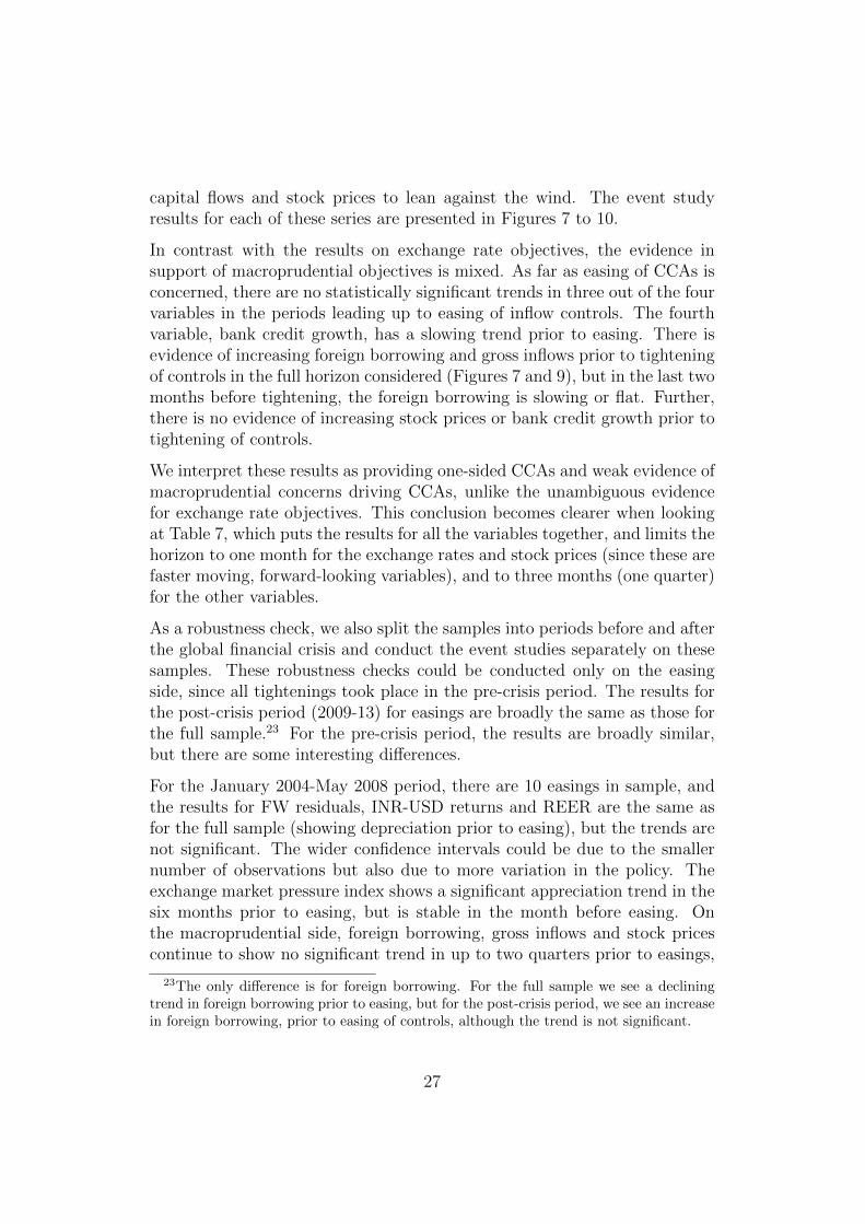
capital flows and stock prices to lean against the wind. The event studyresults for each of these series are presented in Figures 7 to 10.

In contrast with the results on exchange rate objectives, the evidence insupport of macroprudential objectives is mixed. As far as easing of CCAs isconcerned, there are no statistically significant trends in three out of the fourvariables in the periods leading up to easing of inflow controls. The fourthvariable, bank credit growth, has a slowing trend prior to easing. There isevidence of increasing foreign borrowing and gross inflows prior to tighteningof controls in the full horizon considered (Figures 7 and 9), but in the last twomonths before tightening, the foreign borrowing is slowing or flat. Further,there is no evidence of increasing stock prices or bank credit growth prior totightening of controls.

We interpret these results as providing one-sided CCAs and weak evidence ofmacroprudential concerns driving CCAs, unlike the unambiguous evidencefor exchange rate objectives. This conclusion becomes clearer when lookingat Table 7, which puts the results for all the variables together, and limits thehorizon to one month for the exchange rates and stock prices (since these arefaster moving, forward-looking variables), and to three months (one quarter)for the other variables.

As a robustness check, we also split the samples into periods before and afterthe global financial crisis and conduct the event studies separately on thesesamples. These robustness checks could be conducted only on the easingside, since all tightenings took place in the pre-crisis period. The results forthe post-crisis period (2009-13) for easings are broadly the same as those forthe full sample.23 For the pre-crisis period, the results are broadly similar,but there are some interesting differences.

For the January 2004-May 2008 period, there are 10 easings in sample, andthe results for FW residuals, INR-USD returns and REER are the same asfor the full sample (showing depreciation prior to easing), but the trends arenot significant. The wider confidence intervals could be due to the smallernumber of observations but also due to more variation in the policy. Theexchange market pressure index shows a significant appreciation trend in thesix months prior to easing, but is stable in the month before easing. Onthe macroprudential side, foreign borrowing, gross inflows and stock pricescontinue to show no significant trend in up to two quarters prior to easings,

23The only difference is for foreign borrowing. For the full sample we see a decliningtrend in foreign borrowing prior to easing, but for the post-crisis period, we see an increasein foreign borrowing, prior to easing of controls, although the trend is not significant.

27

as seen for the full sample. However, bank credit growth shows significanttrends prior to easings but in the opposite direction. This suggests that notonly was policy not countercyclical, it was procyclical at this time. Theseresults seem to bolster our finding that the policy was not systematicallydriven by macroprudential motivations.

A careful look at the changes allows us to better understand the results forthe pre-crisis period. The new ECB regime came into place in 2004, and thechanges during 2004-05 seem to be structural changes related to the overallliberalization of the policy. The changes in this period included new typesof borrowers under the approval and automatic routes and expansion of thelist of allowable end uses. These changes do not seem to be a response tothe prevailing macroeconomic conditions, but rather, they seem to reflect theestablishment of a new regime of foreign borrowing. If we remove the 2004-05period, and include the crisis period during which the countercyclicality ofpolicy would have been a priority (January 2006-December 2008), the resultsare similar to what we obtained for the full sample. As with the full sample,policy seems acyclical (rather than procyclical as seen in the January 2004-May 2008 period) with respect to systemic risk variables, with no significanttrends in foreign borrowing and bank credit growth, and a barely significant,small decline in stock prices. We see a significant declining trend prior toeasing only in gross inflows. For the exchange rate objective, as with the fullsample, a depreciation trend is seen in all four variables prior to easing, andit is significant for three out of the four variables.

On the whole, the robustness check confirms our results of the primacy ofthe exchange rate objective over the macroprudential objective, both in thehigh-growth pre-crisis period, during the crisis and in the post-crisis periodof less-robust growth.

To summarize, evidence from the logit model and the event studies shows aclear role for exchange rate policy in explaining the RBI’s use of CCAs. Theevidence is less conclusive for variables that may capture macroprudentialobjectives. These variables are not significant in logit regressions. Further,there are no clear patterns in foreign borrowing or stock price returns prior tochanges in controls. We find evidence that easing of controls follows periodsof slowing bank credit growth, but the reverse is not true prior to tightenings.There is evidence of tightening of capital controls during periods of increasinggross inflows, but the reverse is not true prior to easings, and moreover,foreign borrowing itself slows in the two months prior to the change. Puttingthese together, it is hard to conclude that RBI is using CCAs as a tool forsystemic risk reduction. Our results suggest that CCAs may be a tool of

28

exchange rate policy.

Figure 3 INR/USD fluctuations prior to dates of CCAs

−12 −8 −4 0

−5

05

(Cum

.) c

hang

e in

INR

/US

D (

%)

−12 −8 −4 0

Event time (weeks)

● ●● ● ● ● ● ●

●●

●● ●

Response series95 % confidence interval

(a) 68 easing events

−12 −8 −4 0

−5

05

(Cum

.) c

hang

e in

INR

/US

D (

%)

−12 −8 −4 0

Event time (weeks)

● ● ●●

● ● ●

●

● ● ● ● ●


(b) 8 tightening events

29

Figure 4 Frankel-Wei (FW) residual fluctuations prior to dates of CCAs

−12 −8 −4 0

−6

−2

24

6

(Cum

.) c

hang

e in

FW

res

id. (

%)

−12 −8 −4 0

Event time (weeks)

● ● ● ● ● ●● ●

●●

●● ●



−12 −8 −4 0

−6

−2

24

6

(Cum

.) c

hang

e in

FW

res

id. (

%)

−12 −8 −4 0

Event time (weeks)

● ● ●● ● ● ●

●

● ● ●● ●



Figure 5 Fluctuations in the exchange market pressure (EMP) index priorto dates of CCAs

−3.0 −2.0 −1.0 0.0

−20

−10

010

20

(Cum

.) c

hang

e in

EM

P (

%)

−3.0 −2.0 −1.0 0.0

Event time (months)

● ●

●

●



−3.0 −2.0 −1.0 0.0

−20

−10

010

20

(Cum

.) c

hang

e in

EM

P (

%)

−3.0 −2.0 −1.0 0.0

Event time (months)

●

●

● ●



30

Figure 6 Real effective exchange rate (REER) fluctuations prior to dates ofCCAs

−3.0 −2.0 −1.0 0.0

−6

−4

−2

02

46

(Cum

.) c

hang

e in

RE

ER

(%

)

−3.0 −2.0 −1.0 0.0

Event time (months)

●●

●

●



−3.0 −2.0 −1.0 0.0

−6

−4

−2

02

46

(Cum

.) c

hang

e in

RE

ER

(%

)

−3.0 −2.0 −1.0 0.0

Event time (months)

●●

●

●



Figure 7 Fluctuations in foreign borrowings prior to dates of CCAs

−6 −4 −2 0

−0.

3−

0.1

0.1

0.3

(Cum

.) c

hang

e in

EC

B

−6 −4 −2 0

Event time (months)

●

●

●●

●●

●



−6 −4 −2 0

−0.

3−

0.1

0.1

0.3

(Cum

.) c

hang

e in

EC

B

−6 −4 −2 0

Event time (months)

●

●

● ●

●

●●



31

Figure 8 Fluctuations in bank credit growth prior to dates of CCAs

−6 −4 −2 0

−3

−1

01

23

(Cum

.) c

hang

e in

non

−fo

od c

redi

t

−6 −4 −2 0

Event time (months)

●

●

●

●

●● ●



−6 −4 −2 0

−3

−1

01

23

(Cum

.) c

hang

e in

non

−fo

od c

redi

t

−6 −4 −2 0

Event time (months)

● ●● ●

●

● ●



Figure 9 Fluctuations in capital flows prior to dates of CCAs

−5 −4 −3 −2 −1 0

−40

020

40

(Cum

.) c

hang

e in

gro

ss fl

ows

(%)

−5 −4 −3 −2 −1 0

Event time (quarters)

●●

● ●●

●



−5 −4 −3 −2 −1 0

−40

020

40

(Cum

.) c

hang

e in

gro

ss fl

ows

(%)

−5 −4 −3 −2 −1 0


●

●●

●●

●



32

Figure 10 Fluctuations in stock prices prior to dates of CCAs

−12 −8 −4 0

−20

010

20

(Cum

.) c

hang

e in

Nift

y (%

)

−12 −8 −4 0

Event time (weeks)

● ● ● ● ● ● ● ● ● ● ● ● ●



−12 −8 −4 0

−20

010

20

(Cum

.) c

hang

e in

Nift

y (%

)

−12 −8 −4 0

Event time (weeks)

● ●●

● ●

● ●●

●●

●● ●



Table 7 Event study for capital controls motivation: Summary table

Variable Trend prior toExchange rate objective Easing TighteningINR/USD returns Depreciation AppreciationFrankel-Wei residuals Depreciation AppreciationExchange market pressure Depreciation AppreciationREER Depreciation* Appreciation*

Macroprudential objective Easing TighteningForeign borrowing (ECB) No trend No trendBank credit growth Slowing No trendGross inflows No trend IncreasingStock prices No trend No trendNotes: The table summarizes the statistically significant trends (95%)over one month prior to the event for exchange rates and stock prices,and three months (one quarter) prior to the event for the other variables.These horizons are shorter than the ones presented in the figures. * Thetrends in REER are not statistically significant over the one-month hori-zon, but are statistically significant over a two-month horizon. Foreignborrowing first increases then declines over the three months prior totightening dates.

33

7 Results: Were the CCAs effective?

7.1 Event study approach

The event study on effectiveness reveals mixed results for the impact onthe exchange rate (Table 8 and Figures 11 to 14). On both the easing andtightening side, for three outcome variables — INR/USD returns, Frankel-Wei residuals and REER — the post-event mean is no different from themean at the event date.24 Putting this result in the context of results from theprevious section, which showed a steady depreciation trend prior to easing,one could infer that CCAs are able to halt the slide in the exchange rate.However, there is no impact on the exchange market pressure, i.e., the pre-event trend continues unabated post event, for both easing and tighteningevents. This suggests that the halt in spot exchange rate depreciation maysimply reflect greater use of foreign exchange reserves following the event,rather than an impact of the event itself.25 All together, the results are atbest ambiguous and we do not view them as suggesting a clear benefit (interms of exchange rate management) from the use of capital controls.

For the variables representing macroprudential objectives, the evidence forthe effectiveness of capital controls is also thin (Figures 15 to 18). Easing ofcontrols does not have any impact on foreign borrowing (which increases atmonth 1 after the event but falls back thereafter) or gross inflows. Further,the growth of bank credit continues its pre-easing downward trend. Stockprices, however, do show a small increase in the three days after the easingof controls, suggesting the possibility of a positive but short-lived confidenceeffect.

Tightening of capital controls is associated with a significant decline in foreignborrowing in the five months after tightening events. Further, tightening ofcapital controls are followed by strong growth in bank credit (from no trendprior to the event). Together, the two results could suggest a decline inriskiness of overall credit growth with foreign currency borrowing replacedby domestic currency borrowing. However, gross inflows continue to increaseover this period (two quarters). While these trends could be consistent with

24The results on the insignificant difference in mean returns of the spot exchange ratepost-event are not driven by higher volatility of the exchange rate post-event. See Ap-pendix B.

25This conclusion has been verified through an event study on foreign exchange reserves.Prior to easings, foreign exchange reserves were declining and they continued to declinepost-easing. The reverse held for tightening events.

34

the desired outcome of the change in relative composition of inflows towardless-risky forms, they could also be due to a mislabelling of flows as a meansto evade tighter controls. Further, there are very few tightening events inthe sample, and we do not obtain parallel results with the more numerouseasing of controls, which have no impact on each of these series. There isa short-lived decline in stock prices in the three days after tightening, afterwhich there is no impact. For these reasons, we view the evidence in favourof capital controls mitigating macroprudential concerns as being scant.26

To summarize, the event study reveals that post-event, the outcome variableson the whole do not show trends that one would expect if capital controlswere effective. There is some evidence of a stemming of depreciation pres-sures on the currency post-easing, a stemming of appreciation pressures post-tightening and reduced foreign currency borrowing post-tightening. However,we do not know if these trends reflect the impact of controls per se, or whetherthey would have materialized even if capital controls had not been changedwhen they were. To be confident that these results reflect a causal impact ofcapital controls, we need to take the next step, of using a control group ofperiods that were similar to the pre-event periods but where the treatment(CCA) was not applied. The next section presents the results of this analysis.

26As done for the motivations section, we did a robustness check with pre- and post-global financial crisis periods for the easings. The results for the 2006-08 and 2009-13periods are similar to those for the entire sample. In some cases, the evidence of inef-fectiveness is stronger, as the pre-CCA trends in exchange rate variables are not abatedbut continue after the CCA. In the January 2004-May 2008 pre-crisis period, there aresome differences, but these do not change the overall conclusion of ineffectiveness. Theresults are similar for exchange rate variables. Foreign borrowing and gross inflows ini-tially increase post-easing, but these increases are quickly reversed. Bank credit growthrises post-easing in line with the expected impact, whereas stock prices show no significanttrends.

35

Table 8 Event study for capital controls effectiveness: Summary table

Variable Trend afterExchange rate objective Easing TighteningINR/USD returns Halt depreciation Halt appreciationFrankel-Wei residuals Halt depreciation Halt appreciationExchange market pressure Continued depreciation Continued appreciationREER Halt depreciation* Halt appreciation*

Macroprudential objective Easing TighteningForeign borrowing (ECB) No trend (no impact) DeclineBank credit growth Continued decline IncreaseGross inflows No trend (no impact) Continued increaseStock prices No trend (no impact) No trend (no impact)Notes: The table summarizes the statistically significant trends (95%) over sevendays for INR/USD returns, Frankel-Wei residuals and stock prices, three months forREER and the exchange market pressure index, and six months/two quarters forthe other variables. * For REER, the results can be interpreted as halting deprecia-tion/appreciation only if the pre-event horizon is two months.

Figure 11 INR/USD fluctuations after the dates of CCAs

0 1 2 3 4 5 6 7

−4

−2

02

4−

4−

20

24

(Cum

.) c

hang

e in

INR

/US

D (

%)

0 1 2 3 4 5 6 7

Event time (days)

● ●● ● ● ● ● ●



0 1 2 3 4 5 6 7

−4

−2

02

4−

4−

20

24

(Cum

.) c

hang

e in

INR

/US

D (

%)

0 1 2 3 4 5 6 7

Event time (days)

● ●● ● ●

●●

●



36

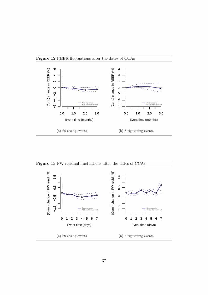
Figure 12 REER fluctuations after the dates of CCAs

0.0 1.0 2.0 3.0

−6

−4

−2

02

46

−6

−4

−2

02

46

(Cum

.) c

hang

e in

RE

ER

(%

)

0.0 1.0 2.0 3.0

Event time (months)

● ●● ●



0.0 1.0 2.0 3.0

−6

−4

−2

02

46

−6

−4

−2

02

46

(Cum

.) c

hang

e in

RE

ER

(%

)0.0 1.0 2.0 3.0

Event time (months)

●● ●

●



Figure 13 FW residual fluctuations after the dates of CCAs

0 1 2 3 4 5 6 7

−1.

5−

0.5

0.5

1.5

−1.

5−

0.5

0.5

1.5

(Cum

.) c

hang

e in

FW

res

id. (

%)

0 1 2 3 4 5 6 7

Event time (days)

●● ●

● ●● ●

●



0 1 2 3 4 5 6 7

−1.

5−

0.5

0.5

1.5

−1.

5−

0.5

0.5

1.5

(Cum

.) c

hang

e in

FW

res

id. (

%)

0 1 2 3 4 5 6 7

Event time (days)

● ● ●

●

●

●

●

●



37

Figure 14 Movements in exchange market pressure after the dates of CCAs

0.0 1.0 2.0 3.0

−20

−10

010

20−

20−

100

1020

(Cum

.) c

hang

e in

EM

P (

%)

0.0 1.0 2.0 3.0

Event time (months)

●

●●

●



0.0 1.0 2.0 3.0

−20

−10

010

20−

20−

100

1020

(Cum

.) c

hang

e in

EM

P (

%)

0.0 1.0 2.0 3.0

Event time (months)

●

●

●●



Figure 15 Fluctuations in foreign borrowings after the dates of CCAs

0 1 2 3 4 5 6

−0.

3−

0.1

0.1

0.3

−0.

3−

0.1

0.1

0.3

(Cum

.) c

hang

e in

EC

B

0 1 2 3 4 5 6

Event time (months)

●

●

● ● ● ● ●



0 1 2 3 4 5 6

−0.

3−

0.1

0.1

0.3

−0.

3−

0.1

0.1

0.3

(Cum

.) c

hang

e in

EC

B

0 1 2 3 4 5 6

Event time (months)

●●

●●

● ●

●



38

Figure 16 Fluctuations in overall capital flows after the dates of CCAs

0 1 2 3 4 5

−40

020

40−

400

2040

(Cum

.) c

hang

e in

gro

ss fl

ows

(%)

0 1 2 3 4 5


●● ● ●

● ●



0 1 2 3 4 5

−40

020

40−

400

2040

(Cum

.) c

hang

e in

gro

ss fl

ows

(%)

0 1 2 3 4 5


●

●

●

●

●

●



Figure 17 Fluctuations in bank credit growth after the dates of CCAs

0 1 2 3 4 5 6

−3

−1

01

23

−3

−1

01

23

(Cum

.) c

hang

e in

non

−fo

od c

redi

t

0 1 2 3 4 5 6

Event time (months)

●●

●

●

●● ●



0 1 2 3 4 5 6

−3

−1

01

23

−3

−1

01

23

(Cum

.) c

hang

e in

non

−fo

od c

redi

t

0 1 2 3 4 5 6

Event time (months)

●●

●

●

●

●●



39

Figure 18 Fluctuations in stock prices after the dates of CCAs

0 1 2 3 4 5 6 7

−4

−2

02

4−

4−

20

24

(Cum

.) c

hang

e in

Nift

y (%

)

0 1 2 3 4 5 6 7

Event time (days)

●

●●

●●

●● ●



0 1 2 3 4 5 6 7

−4

−2

02

4−

4−

20

24

(Cum

.) c

hang

e in

Nift

y (%

)

0 1 2 3 4 5 6 7

Event time (days)

●

●

●

●●

●

●●



7.2 Causal analysis using propensity score matching

The results of section 6 show that the RBI utilizes a certain selectivity processthat determines when a CCA is employed. The time periods prior to the weekof a CCA have certain characteristics. We use propensity score matching toidentify similar time periods, when no CCA was employed. This gives acontrol time period (see Appendix D). The explanatory variables used inthe logit model are the same as those in model 1 in Table 6: exchange ratechanges, credit growth, money supply growth and returns on Nifty.27

While only a small set of explanatory variables were used in the logit model,match balance is achieved for a broad set of time-series variables, as shown inTable 9. In this table, the null of equality of distributions is always rejectedbefore matching and is broadly not rejected after matching. This suggeststhat we have succeeded in finding a set of 22 control weeks when macroeco-nomic conditions were much like the 22 treatment weeks. Figure 19 showsthat the cumulative density of the propensity scores is highly unequal beforematching, but after the matching, the two distributions are alike, indicatingthat there is match balance.

Using this matched sample of 22 weeks with a CCA and 22 weeks with noCCA, we conduct an event study about returns on the INR/USD exchangerate. This result is shown in Figure 20. The difference in returns between

27Our results are robust to using model 2 in Table 6.

40

each pair is averaged and cumulated. We know from Figure 3 that rupeedepreciation took place in the weeks prior to a CCA. Since the control weeksare similar, rupee depreciation also took place in the weeks prior to thesimilar date with no CCA. Hence, we see no significant difference prior tothe event date in the event study. Turning to the period after the event date,we see no statistically significant impact, since there is no difference betweenthe treatment week and the control week.28

Figure 19 Cumulative density function of the propensity scores before andafter matching

0.0 0.2 0.4 0.6 0.8

0.0

0.4

0.8

Before Matching

Cum

ulat

ive

dens

ity

TreatedControl

0.0 0.1 0.2 0.3 0.4 0.5 0.6 0.7

0.0

0.4

0.8

After Matching

Cum

ulat

ive

dens

ity

TreatedControl

Table 10 applies such causal analysis to multiple outcome measures. Whetherwe look at the residuals of the Frankel-Wei regression, the stock market indexor credit growth, there is no statistically significant impact.

28Our results on effectiveness are robust to using the genetic matching algorithm, asdescribed in the methodology section.

41

Table 9 Kolmogorov-Smirnov test for equality of distributionsThe table shows the Kolmogorov-Smirnov test result for a broad set of variables for thetreated and control group before and after matching. The values in parentheses are p-values. FII refers to foreign institutional investors.

Before Matching After MatchingPropensity score 0.49 0.09

(0) (1)INR/USD returnst−1 0.33 0.23

(0.01) (0.63)Bank credit growtht−1 0.11 0.09

(0.88) (1)M3 growtht−1 0.11 0.23

(0.87) (0.62)Nifty returnst−1 0.28 0.41

(0.03) (0.05)FW predictedt−1 0.09 0.14

(0.97) (0.99)FW residualst−1 0.33 0.23

(0.01) (0.63)Net FII inflowst−1 0.35 0.33

(0.01) (0.22)INR/USD returnst−2 0.32 0.32

(0.01) (0.22)Bank credit growtht−2 0.05 0.14

(1) (0.99)M3 growtht−2 0.13 0.18

(0.7) (0.86)Nifty returnst−2 0.22 0.18

(0.13) (0.87)FW predictedt−2 0.24 0.36

(0.11) (0.11)FW residualst−2 0.3 0.18

(0.02) (0.87)Net FII inflowst−2 0.16 0.54

(0.68) (0.01)INR/USD returnst−3 0.45 0.23

(0) (0.63)Bank credit growtht−3 0.11 0.14

(0.9) (0.99)M3 growtht−3 0.07 0.09

(1) (1)Nifty returnst−3 0.29 0.23

(0.02) (0.63)FW predictedt−3 0.17 0.27

(0.5) (0.36)FW residualst−3 0.34 0.17

(0.01) (0.84)Net FII inflowst−3 0.12 0.32

(0.92) (0.24)

42

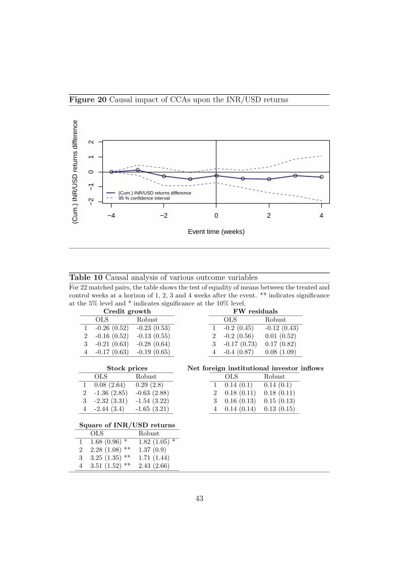
Figure 20 Causal impact of CCAs upon the INR/USD returns

−4 −2 0 2 4

−2

−1

01

2

Event time (weeks)

(Cum

.) IN

R/U

SD

ret

urns

diff

eren

ce

● ●

●●

●● ●

● ●

(Cum.) INR/USD returns difference95 % confidence interval

Table 10 Causal analysis of various outcome variablesFor 22 matched pairs, the table shows the test of equality of means between the treated andcontrol weeks at a horizon of 1, 2, 3 and 4 weeks after the event. ** indicates significanceat the 5% level and * indicates significance at the 10% level.

Credit growth FW residualsOLS Robust

1 -0.26 (0.52) -0.23 (0.53)2 -0.16 (0.52) -0.13 (0.55)3 -0.21 (0.63) -0.28 (0.64)4 -0.17 (0.63) -0.19 (0.65)

OLS Robust1 -0.2 (0.45) -0.12 (0.43)2 -0.2 (0.56) 0.01 (0.52)3 -0.17 (0.73) 0.17 (0.82)4 -0.4 (0.87) 0.08 (1.09)

Stock prices Net foreign institutional investor inflowsOLS Robust

1 0.08 (2.64) 0.29 (2.8)2 -1.36 (2.85) -0.63 (2.88)3 -2.32 (3.31) -1.54 (3.22)4 -2.44 (3.4) -1.65 (3.21)

OLS Robust1 0.14 (0.1) 0.14 (0.1)2 0.18 (0.11) 0.18 (0.11)3 0.16 (0.13) 0.15 (0.13)4 0.14 (0.14) 0.13 (0.15)

Square of INR/USD returnsOLS Robust

1 1.68 (0.96) * 1.82 (1.05) *2 2.28 (1.08) ** 1.37 (0.9)3 3.25 (1.35) ** 1.71 (1.44)4 3.51 (1.52) ** 2.43 (2.66)

43

8 Summary and Conclusions

There is renewed interest in reassessing the potential role for capital controlsas a tool for macroeconomic or macroprudential policy. In well-structuredfinancial regulatory regimes, regulations that restrict capital account trans-actions would ideally be precisely stated and backed by cost-benefit analysis.

Of particular importance are comprehensive administrative systems thatcover all kinds of capital account transactions, since the evidence shows thatthe episodic use of capital controls in an otherwise open capital account haslow effectiveness. Within the broad range of restrictions, there is particularinterest in restricting foreign borrowing, given the potential implications forsystemic risk.

Four important unanswered questions can be identified. First, what are cap-ital controls? Second, when do policy-makers actually use capital controls?Third, what is the causal impact of various kinds of CCAs? Finally, do thebenefits of capital controls outweigh their costs?

In this paper, we study one large country, India, which is a rare example of acomprehensive administrative system of capital controls. Such a comprehen-sive system is advocated in some of the recent proposals to resurrect capitalcontrols. We focus on one class of restrictions — on foreign borrowing —which could be important from the viewpoint of systemic risk.

Building on the recent work of Pasricha (2012) and Forbes et al. (2013), weanalyze individual CCAs, rather than the low-frequency measures of capitalaccount openness that have dominated the traditional literature. We improveupon existing work by undertaking a thorough legal analysis of every CCA,and arrive at a new data set of 76 CCAs. An avenue for future research is tobuild a similar standardized classification system for multiple countries thatwould allow similar cross-country studies of capital controls.

Our analysis yields two main results. First, the Indian authorities seem toemploy CCAs primarily in response to exchange rate movements. In partic-ular, they seem to respond to the country-specific component of exchangerate movements.

The second result is about the impact of these capital control actions. Thetreatment effect is analyzed in two ways: event study and propensity scorematching. Both kinds of analysis show that the CCAs have no robust impact.This result is consistent with the recent literature on capital controls in India(Patnaik and Shah, 2012) and in other countries (Jinjarak et al., 2013).

44

Our results are also consistent with the mainstream capital controls literaturefrom the 1980s and 1990s. The Indian authorities seem to be utilizing CCAsto pursue exchange rate policy and not for systemic risk reduction, and theiractions do not seem to be effective in influencing either the exchange rate orother outcomes.

45

References

Aggarwal, N. and S. Thomas (2013). Market quality in the time of algorith-mic trading. Technical Report December, IGIDR FRG.

Aizenman, J. and G. K. Pasricha (2013). Why do emerging markets liberalizecapital outflow controls? fiscal versus net capital flow concerns. Journalof International Money and Finance 39 (C), 28–64.

Anand, C., V. Bahure, V. Balasubramaniam, and A. Shah (2014). eventstud-ies: An R package for researchers and users of event studies. NIPFP.

Angrist, J. and J. Hahn (2004). When to control for covariates? panelasymptotics for estimates of treatment effects. Review of Economics andStatistics 86 (1), 58–72.

Angrist, J. and J.-S. Pischke (2008). Mostly Harmless Econometrics: AnEmpiricist’s Companion. Princeton University Press.

Angrist, J. D. and G. M. Kuersteiner (2011). Causal effects of monetaryshocks: semiparametric conditional independence tests with a multinomialpropensity score. The Review of Economics and Statistics 93 (3), 725–747.

Bank of England (2009). The role of macroprudential policy. Bank of EnglandDiscussion Paper 19 November 2009.

BIS, FSB, and IMF (2011, February). Macroprudential policy tools andframeworks: Update to G20 finance ministers and central bank governors.Technical report, Bank for International Settlements.

Blanchard, O. (2013). Monetary policy will never be the same. iMFDirect 19November.

Blundell-Wignall, A. and C. Roulet (2013). Capital controls on inflows,the global financial crisis and economic growth: Evidence for emergingeconomies. OECD Journal: Financial Market Trends 2.

Caliendo, M. and S. Kopeinig (2005). Some practical guidance for the imple-mentation of propensity score matching. Discussion Paper 1588, Institutefor the Study of Labor (IZA).

Carvalho, B. S. d. M. and M. G. P. Garcia (2008). Ineffective controls oncapital inflows under sophisticated financial markets: Brazil in the nineties.In S. Edwards and M. G. P. Garcia (Eds.), Financial Markets Volatility

46

and Performance in Emerging Markets, pp. 29–96. University of ChicagoPress.

Chinn, M. and H. Ito (2008). A new measure of financial openness. Journalof Comparative Policy Analysis 10 (3), 309–322.

Davison, A. C., D. V. Hinkley, and E. Schechtman (1986). Efficient bootstrapsimulation. Biometrika 73 (3), 555–566.

Edwards, S. (1999). How effective are capital controls? NBER WorkingPapers 7413, National Bureau of Economic Research, Inc.

Edwards, S. and J. D. Ostry (1992, January). Terms of trade disturbances,real exchange rates, and welfare: The role of capital controls and labormarket distortions. Oxford Economic Papers 44 (1), 20–34.

Eichengreen, B., R. Hausmann, and U. Panizza (2007). Currency mis-matches, debt intolerance, and the original sin: Why they are not the sameand why it matters. In Capital Controls and Capital Flows in EmergingEconomies: Policies, Practices and Consequences, NBER Chapters, pp.121–170. National Bureau of Economic Research, Inc.

Felman, J. and I. Patnaik (2013). Did QE Unleash a Monetary Tsunami? AnExchange Market Pressure Approach. Technical report, National Instituteof Public Finance and Policy.

Forbes, K., M. Fratzscher, and R. Straub (2013). Capital controls and macro-prudential measures: What are they good for? Discussion Papers of DIWBerlin 1343, DIW Berlin, German Institute for Economic Research.

Forbes, K. J. (2004). Capital controls: Mud in the wheels of market discipline.Working papers 4454-03, Massachusetts Institute of Technology (MIT),Sloan School of Management.

Forbes, K. J. (2005). The microeconomic evidence on capital controls: Nofree lunch. NBER Working Papers 11372, National Bureau of EconomicResearch, Inc.

Frankel, J. and S.-J. Wei (1994). Yen bloc or dollar bloc? Exchange rate poli-cies of the East Asian countries. In T. Ito and A. Krueger (Eds.), Macroe-conomic Linkage: Savings, Exchange Rates and Capital Flows. Universityof Chicago Press.

Fratzscher, M. (2012). Capital controls and foreign exchange policy. WorkingPaper 1415, European Central Bank.

47

Goldstein, M. and P. Turner (2004). Controlling Currency Mismatches inEmerging Markets. Number 373 in Peterson Institute Press: All Books.Peterson Institute for International Economics.

Haldane, A. G. and S. G. Hall (1991). Sterling’s relationship with the dollarand the deutschemark: 1976–89. The Economic Journal 101, 436–443.

Hutchison, M. M., G. K. Pasricha, and N. Singh (2012). Effectiveness ofcapital controls in India: Evidence from the offshore NDF market. IMFEconomic Review 60 (3), 395–438.

IMF (2012). The liberalization and management of capital flows - an insti-tutional view. Policy paper, International Monetary Fund.

Jadhav, N. (2003). Capital account liberalisation: the indian experience.Reserve Bank of India (Mumbai).

Jinjarak, Y., I. Noy, and H. Zheng (2013). Capital controls in brazil–stemming a tide with a signal? Journal of Banking & Finance 37 (8),2938–2952.

Klein, M. W. (2012). Capital controls: Gates versus walls. Brookings Paperson Economic Activity 45 (2 (Fall)), 317–367.

Kothari, S. and J. Warner (2007). Econometrics of event studies. In B. E.Eckbo (Ed.), Handbook of Corporate Finance, Volume 1, Chapter 1, pp.29–96. Elsevier.

Magud, N. E., C. M. Reinhart, and K. S. Rogoff (2011). Capital Controls:Myth and Reality - A Portfolio Balance Approach. Working Paper 16805,National Bureau of Economics Research.

Moura, M. L., F. R. Pereira, and G. de Moraes Attuy (2013). Currencywars in action: How foreign exchange interventions work in an emergingeconomy. Technical Report March, Insper.

Nier, E., J. Osiski, J. Chen, H. Kang, Y. Kim, I. Krznar, R. D. Mooji,M. Keen, L. Ratnoski, and P. Kongsamut (2013). Key aspects of macro-prudential policy. Technical report, IMF Background Paper.

OECD (2012). Recommendation of the council on regulatory policy andgovernance. Report, Organisation for Economic Co-operation and Devel-opment.

48

Ostry, J., A. R. Ghosh, K. Habermeier, M. Chamon, M. S. Qureshi, and D. B.Reinhardt (2010). Capital inflows: The role of controls. Staff Position NoteSPN/10/04, International Monetary Fund.

Ostry, J. D., A. R. Ghosh, M. Chamon, and M. S. Qureshi (2012). Tools formanaging financial-stability risks from capital inflows. Journal of Interna-tional Economics 88 (2), 407 – 421.

Pasricha, G. K. (2012). Recent trends in measures to manage capital flowsin emerging economies. The North American Journal of Economics andFinance 23 (3), 286–309.

Patnaik, I. and A. Shah (2012). Did the Indian capital controls work as atool of macroeconomic policy. IMF Economic Review 60 (3), 439–464.

Patnaik, I., A. Shah, and N. Singh (2013, September). Foreign investorsunder stress: Evidence from india. International Finance 16 (2), 213–244.

Pradhan, M., R. Balakrishnan, R. Baqir, G. Heenan, S. Nowak, C. Oner, andS. Panth (2011). Policy responses to capital flows in emerging markets.Technical report, IMF Staff Discussion Note.

Schindler, M. (2009). Measuring financial integration: A new data set. IMFStaff Papers 56 (1), 222–238.

Sekhon, J. S. (2011). Multivariate and Propensity Score Matching Soft-ware with Automated Balance Optimization: The Matching package forR. Journal of Statistical Software, American Statistical Association 42 (7).

Sinha, U. K. (2010). Working group on foreign investment. Committeereport, Department of Economic Affairs, Ministry of Finance, Governmentof India.

49

A Construction of the CCA database: Two

examples

In this appendix, we present two examples of our methodology for translatingCCAs into a consistent database for evaluating the effectiveness of controls.

1. On 21 May 2007, an RBI circular (http://rbi.org.in/scripts/NotificationUser.aspx?Id=3544&Mode=0) reduced the spread on all-in-cost ceilings to 150 ba-sis points for maturities of three to five years and to 250 basis points formaturities of more than five years. The reduced spread was also announcedfor borrowers under the approval route. End-use requirements governing ex-ternal borrowings were tightened: proceeds from external commercial bor-rowing (ECB) could no longer be used for investing in real estate, includingintegrated townships.

From this circular we get three tightening events:

(a) The all-in-cost ceilings were reduced for eligible borrowers under theautomatic route.

(b) The all-in-cost ceilings were reduced for eligible borrowers under theapproval route.

(c) The end-use restrictions were tightened.

For this date we get three records in the CCA database, all of which aretightening. Pasricha (2012) classifies these three events introduced on a sin-gle day as two tightening events: it groups the two price-based measures(cost-ceiling changes) as one event and categorizes the end-use restrictionsas a quantitative event. These changes may have differential impact on thedifferent types of borrowers (firms under approval and automatic routes).Hence, for the purpose of assessing the impact of controls, they merit inde-pendent counting as three tightening events.

2. On 29 May 2008, an RBI circular (http://rbi.org.in/scripts/NotificationUser.aspx?Id=4200&Mode=0) eased capital controls in three directions:

(a) The restrictions on all-in-cost ceilings were eased to 200 basis pointsfrom 150 basis points for three- to five-year maturities and from 250 to350 basis points over six-month LIBOR for above-five-year maturities.

(b) Borrowers that were infrastructure firms were permitted to borrowthrough ECB with a limit of USD 100 million, for the purpose of rupeeexpenditure, for permissible end uses, under the approval route.

(c) For other borrowers, the existing limit of USD 20 million for rupeeexpenditure for permissible end uses under the approval route wasenhanced to USD 50 million.

50

http://rbi.org.in/scripts/NotificationUser.aspx?Id=3544&Mode=0




For this date we get three records in the CCA database, and all three areeasing. This circular cannot be read independently. The nature of changeintroduced in this circular is different from the previous example. In thiscircular, several of the previous tightening events were reversed. This re-quires tracking all the previous circulars to get an idea of the sequentialliberalization of tightening measures.

From this circular, we get three easing events related to the following aspectsof ECB regulation:

(a) Easing of all-in-cost ceilings.

(b) Easing of restrictions on eligible borrowers under the approval route.

(c) Easing of restrictions on permissible amounts.

Pasricha (2012) counts the cost ceilings as one event and groups the othertwo quantitative changes as one event. In our classification system, theseare viewed as three distinct easing events, since the nature of changes intro-duced through this circular are different and may have differential impactfor different borrowers.

In this way, we do a careful reading of each of the 97 circulars and trackchanges related to all aspects of ECB regulation. This approach sheds lighton the minutest details of changes in capital controls. For example, whileForbes et al. (2013) identifies five events directed toward easing, our ap-proach (that focuses on controls on one category of international capitaltransactions, i.e., external borrowing) is able to identify 14 easing events inthe period 2009-11. The number is likely to go up if we extend this approachto tracking capital controls on all categories of international transactions.

51

B Was currency volatility the driver?

Figure 21 Movements in currency volatility after the dates of CCAs

−5 −4 −3 −2 −1 0 1 2 3 4 5

Event time (days)

Vol

atili

ty o

f IN

R/U

SD

(%

)

0.0

0.5

1.0

1.5

2.0

2.5

Mea

n vo

latil

ity


−5 −4 −3 −2 −1 0 1 2 3 4 5

Event time (days)

Vol

atili

ty o

f IN

R/U

SD

(%

)

0.0

0.5

1.0

1.5

2.0

2.5

Mea

n vo

latil

ity


52

Figure 22 Movements in FW residual volatility after the dates of CCAs

−5 −4 −3 −2 −1 0 1 2 3 4 5

Event time (days)

Vol

atili

ty o

f FW

res

id. (

%)

0.0

0.5

1.0

1.5

2.0

2.5

Mea

n vo

latil

ity


−5 −4 −3 −2 −1 0 1 2 3 4 5

Event time (days)

Vol

atili

ty o

f FW

res

id. (

%)

0.0

0.5

1.0

1.5

2.0

2.5

Mea

n vo

latil

ity


53

C Data sources

Table 11 Data sourcesVariables SourcesRupee-U.S. dollar exchange rate Reserve Bank of IndiaFrankel-Wei residuals India-specific component of fluctuations in

INR/USD exchange rate based onFrankel and Wei (1994) methodology

Exchange market pressure Felman and Patnaik (2013)measure expressed in terms ofper cent change in exchangerate at a monthly frequency

Real effective exchange rate Bank for International SettlementsForeign borrowing Reserve Bank of IndiaPrivate bank credit growth Reserve Bank of IndiaStock price returns National Stock ExchangeGross capital flows Reserve Bank of IndiaMoney supply (M3) Reserve Bank of India

54

D Matching for dates of CCAs

We show the list of weeks with CCAs and the matched week with no CCAthat was identified using propensity score matching.

Treated Control2004-02-06 2004-10-082005-04-29 2005-06-032005-08-05 2003-01-102006-12-08 2005-06-242008-10-31 2009-03-132010-01-29 2003-07-042010-03-05 2009-01-302010-05-14 2005-11-252010-07-23 2009-03-202010-08-13 2006-07-072011-12-23 2004-05-282012-01-06 2009-07-032012-03-02 2011-08-192012-04-20 2010-11-192012-04-27 2004-05-072012-09-14 2007-06-082012-11-09 2010-12-102012-11-30 2009-09-042012-12-14 2006-04-142012-12-21 2008-03-282013-01-11 2011-05-272013-07-12 2012-08-03

55

Motivations for Capital Controls and Their Effectiveness · iii . Abstract . We assess the...

Documents

Transcript of Motivations for Capital Controls and Their Effectiveness · iii . Abstract . We assess the...