Moran’s I Geary’s C - Salisbury Universityfaculty.salisbury.edu/~ajlembo/419/sa.pdf · •...

© Arthur J. Lembo, Jr.Salisbury University

Spatial Autocorrelation

Moran’s IGeary’s C



• First law of geography: “everything is related to everything else, but near things are more related than distant things” – Waldo Tobler

• Many geographers would say “I don’t understand spatial autocorrelation” Actually, they don’t understand the mechanics, they do understand the concept.


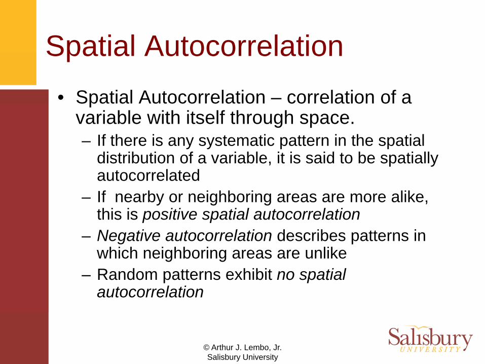
Spatial Autocorrelation• Spatial Autocorrelation – correlation of a

variable with itself through space.– If there is any systematic pattern in the spatial

distribution of a variable, it is said to be spatially autocorrelated

– If nearby or neighboring areas are more alike, this is positive spatial autocorrelation

– Negative autocorrelation describes patterns in which neighboring areas are unlike

– Random patterns exhibit no spatial autocorrelation


Why spatial autocorrelation is important

• Most statistics are based on the assumption that the values of observations in each sample are independent of one another

• Positive spatial autocorrelation may violate this, if the samples were taken from nearby areas

• Goals of spatial autocorrelation– Measure the strength of spatial autocorrelation in

a map – test the assumption of independence or

randomness



• Spatial Autocorrelation is, conceptually as well as empirically, the two-dimensional equivalent of redundancy

• It measures the extent to which the occurrence of an event in an areal unit constrains, or makes more probable, the occurrence of an event in a neighboring areal unit.


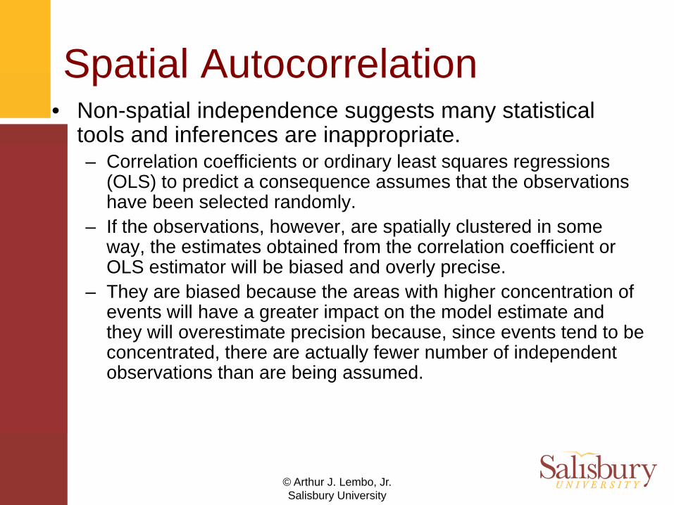
Spatial Autocorrelation• Non-spatial independence suggests many statistical

tools and inferences are inappropriate.– Correlation coefficients or ordinary least squares regressions

(OLS) to predict a consequence assumes that the observations have been selected randomly.

– If the observations, however, are spatially clustered in some way, the estimates obtained from the correlation coefficient or OLS estimator will be biased and overly precise.

– They are biased because the areas with higher concentration of events will have a greater impact on the model estimate and they will overestimate precision because, since events tend to be concentrated, there are actually fewer number of independent observations than are being assumed.


Indices of Spatial Autocorrelation

• Moran’s I• Geary’s C• Ripley’s K• Join Count Analysis


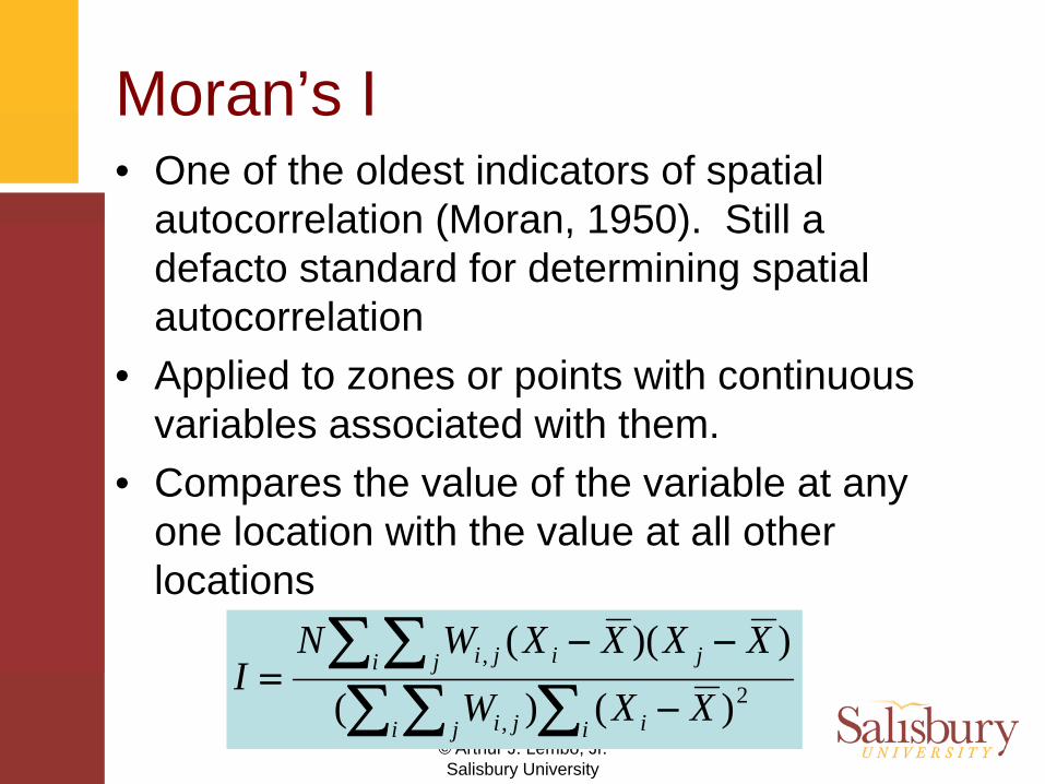
Moran’s I• One of the oldest indicators of spatial

autocorrelation (Moran, 1950). Still a defacto standard for determining spatial autocorrelation

• Applied to zones or points with continuous variables associated with them.

• Compares the value of the variable at any one location with the value at all other locations

∑ ∑ ∑∑ ∑

−

−−=

i j i iji

i j jiji

XXW

XXXXWNI 2

,

,

)()(

))((


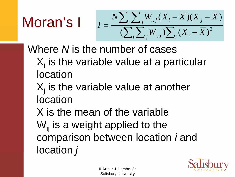
Moran’s I

Where N is the number of casesXi is the variable value at a particular locationXj is the variable value at another locationX is the mean of the variableWij is a weight applied to the comparison between location i and location j

∑∑ ∑∑∑

−

−−=

i j i iji

i j jiji

XXW

XXXXWNI 2

,

,

)()(

))((


Moran’s I• Wij is a contiguity matrix

– If zone j is adjacent to zone i, the interaction receives a weight of 1

– Another option is to make Wij a distance-based weight which is the inverse distance between locations I and j (1/dij)

– Compares the sum of the cross-products of values at different locations, two at a time weighted by the inverse of the distance between the locations

• Similar to correlation coefficient, it varies between –1.0 and + 1.0– When autocorrelation is high, the coefficient is high– A high I value indicates positive autocorrelation


Moran’s I

• Problems with weights– Potential for distorted I value.– Wij is normalized by

ijji

ijji

ijji

dW

dmilemileW

dunitunitW

+=

+=

+=

52805280

,

,

,


Testing the Significance

• Empirical distribution can be compared to the theoretical distribution by dividing by an estimate of the theoretical standard deviation

)(

)()(IESIEIIZ −

=

]))(1(

)()(3[ 22

2222

)( ∑∑ ∑ ∑ ∑

−

−+=

ij ij

ij ij i j ijijijIE wN

wNwwNSQRTS


Example of Moran’s I –Per Capita Income in

Monroe County

Using Polygons:Morans I: .66

P: < .001

Using Points:I: .12Z: 65


Example of Moran’s I –Random Variable

Using Polygons:

Moran’s I: .012p: .515

Using Points:

Moran’s I: .0091Z: 1.36


Geary’s C• Similar to Moran’s I (Geary, 1954)• Interaction is not the cross-product of

the deviations from the mean, but the deviations in intensities of each observation location with one another

∑ ∑∑ ∑

−

−−=

i j iij

i j jiij

XXW

XXWNC 2

2

)((2

])()[1[(


Geary’s C

• Value typically range between 0 and 2• If value of any one zone are spatially unrelated to

any other zone, the expected value of C will be 1– Values less than 1 (between 1 and 2) indicate negative

spatial autocorrelation• Inversely related to Moran’s I• Does not provide identical inference because it emphasizes the

differences in values between pairs of observations, rather than the covariation between the pairs.

• Moran’s I gives a more global indicator, whereas the Geary coefficient is more sensitive to differences in small neighborhoods.

∑ ∑∑ ∑

−

−−=

i j iij

i j jiij

XXW

XXWNC 2

2

)((2

])()[1[(


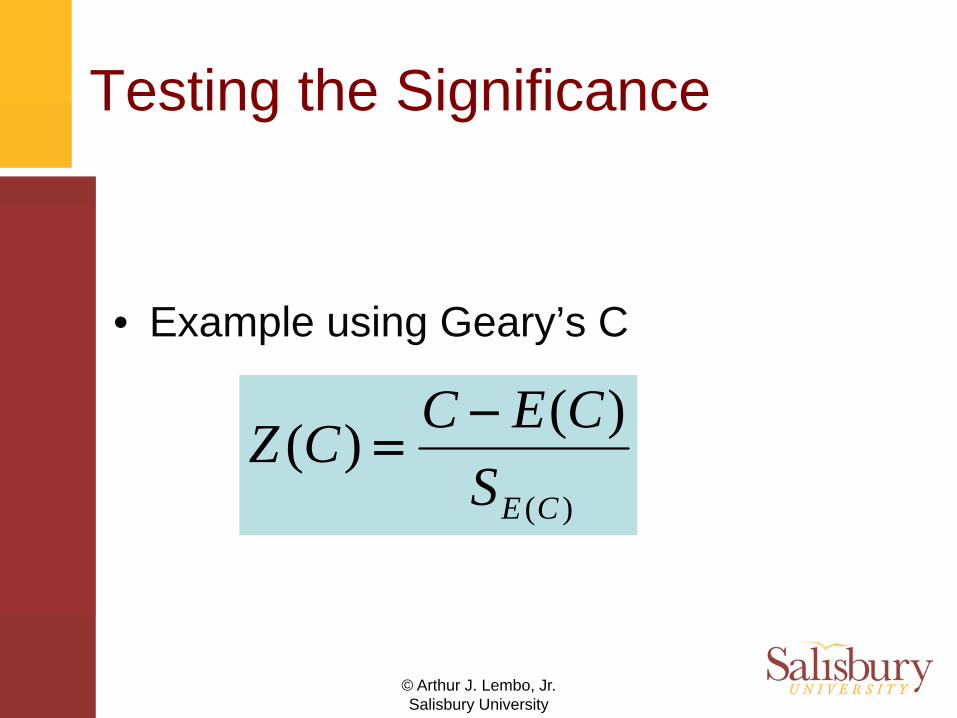
Testing the Significance

• Example using Geary’s C

)(

)()(CESCECCZ −

=



Join Count Analysis


Join Count

• Nominal variables mapped in two colors (B & W). Therefore, the join, or border can be classified as WW, BB, BW

• Different Join Patterns– Rook’s Case– Queen’s Case– Bishop’s Case


A 0 0 24 24

B 5 7 12 24

C 10 10 4 24

Join Counts

Map

BB WW BW Tot.


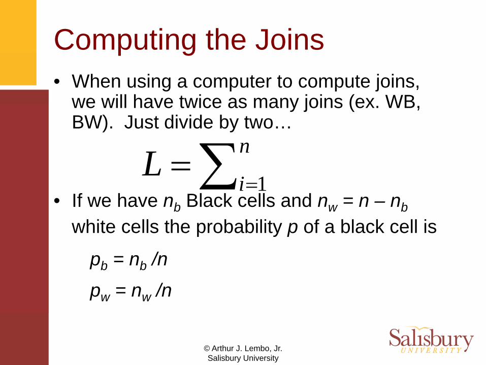
Computing the Joins• When using a computer to compute joins,

we will have twice as many joins (ex. WB, BW). Just divide by two…

• If we have nb Black cells and nw = n – nb

white cells the probability p of a black cell is

pb = nb /npw = nw /n

∑==

n

iL

1


Computing the probabilities

• Start with first cell. The probability it is black is pb and the probability of white is pw

• The probability of BB in two adjacent cells ispb * pb or pb

2

• Probability of BW ispb * pw + pb * pw or 2 pb pw


• Therefore, if there are L joins on a map, the expected number of cells of each type isE(BB) = μ(BB) = pb

2LE(WW) = μ(ww) = pw

2LE(BW) = μ(BW) = 2pbwL


Test Statistics for Join-Count


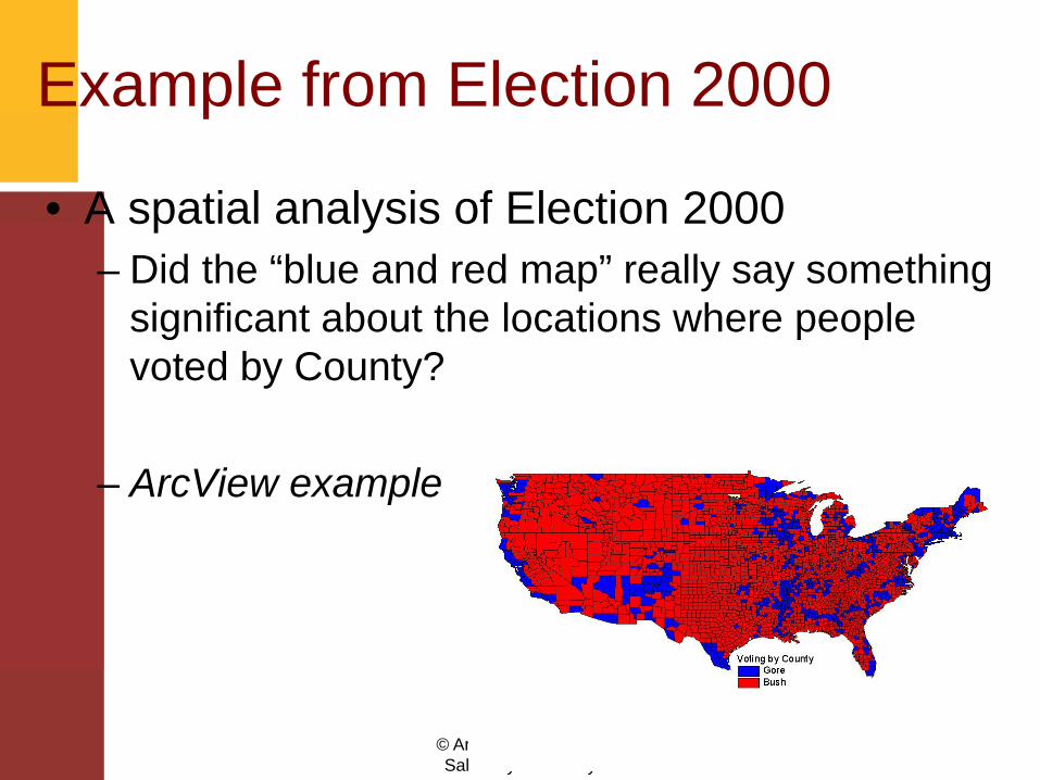
Example from Election 2000

• A spatial analysis of Election 2000– Did the “blue and red map” really say something

significant about the locations where people voted by County?

– ArcView example

Moran’s I Geary’s C - Salisbury Universityfaculty.salisbury.edu/~ajlembo/419/sa.pdf · •...

Documents

Transcript of Moran’s I Geary’s C - Salisbury Universityfaculty.salisbury.edu/~ajlembo/419/sa.pdf · •...