Monte Carlo Generators for Tau-Charm-Physics at...

BAD 522 V6Based on EvtGen V00-11-07

Monte Carlo Generators for Tau-Charm-Physics

at BESIII

Rong -Gang Ping ([email protected])Cai -Ying Pang ([email protected])

December 4, 2006

Abstract

This note describes two kinds of Mont-Carlo generator at BESIII. One is inheritedfrom BESII and the other is that based on the amplitude information developed fromEvtGen. We focus on the description on the model for the latter, especially for theconstruction of the amplitude. The models cover the hadronic decays, radiative decaysand decays for investigating some physical quantities in charmonium physics. The useris suggested to refer the guide of the EvtGen for some generators applicable to bothcharm and B physics.

1

Contents

1 Introduction 6

2 EvtGen Framwork 62.1 Particle properties in EvtGen . . . . . . . . . . . . . . . . . . . . . . . . . . 62.2 Particle representation . . . . . . . . . . . . . . . . . . . . . . . . . . . . . . 62.3 Conventions . . . . . . . . . . . . . . . . . . . . . . . . . . . . . . . . . . . . 9

2.3.1 Units . . . . . . . . . . . . . . . . . . . . . . . . . . . . . . . . . . . . 92.3.2 Four-vectors . . . . . . . . . . . . . . . . . . . . . . . . . . . . . . . . 92.3.3 Tensors . . . . . . . . . . . . . . . . . . . . . . . . . . . . . . . . . . 92.3.4 Dirac spinors . . . . . . . . . . . . . . . . . . . . . . . . . . . . . . . 92.3.5 Gamma matrices . . . . . . . . . . . . . . . . . . . . . . . . . . . . . 9

2.4 Algorithm . . . . . . . . . . . . . . . . . . . . . . . . . . . . . . . . . . . . . 102.5 Introduction to decay models . . . . . . . . . . . . . . . . . . . . . . . . . . 112.6 Creating new decay models . . . . . . . . . . . . . . . . . . . . . . . . . . . 132.7 Available base classes in EvtGen . . . . . . . . . . . . . . . . . . . . . . . . 13

3 EvtGen developed at BESIII 163.1 Helicity amplitudes . . . . . . . . . . . . . . . . . . . . . . . . . . . . . . . . 163.2 Base classes . . . . . . . . . . . . . . . . . . . . . . . . . . . . . . . . . . . . 17

3.2.1 EvtHelSys . . . . . . . . . . . . . . . . . . . . . . . . . . . . . . . . . 17

4 Decay models for charmonium physics 184.1 JPIPI . . . . . . . . . . . . . . . . . . . . . . . . . . . . . . . . . . . . . . . 184.2 AngSam . . . . . . . . . . . . . . . . . . . . . . . . . . . . . . . . . . . . . . 204.3 P2GC0 . . . . . . . . . . . . . . . . . . . . . . . . . . . . . . . . . . . . . . . 204.4 P2GC1 . . . . . . . . . . . . . . . . . . . . . . . . . . . . . . . . . . . . . . . 214.5 P2GC2 . . . . . . . . . . . . . . . . . . . . . . . . . . . . . . . . . . . . . . . 214.6 AV2GV . . . . . . . . . . . . . . . . . . . . . . . . . . . . . . . . . . . . . . 224.7 T2GV . . . . . . . . . . . . . . . . . . . . . . . . . . . . . . . . . . . . . . . 234.8 J2BB1 . . . . . . . . . . . . . . . . . . . . . . . . . . . . . . . . . . . . . . . 234.9 J2BB2 . . . . . . . . . . . . . . . . . . . . . . . . . . . . . . . . . . . . . . . 244.10 J2BB3 . . . . . . . . . . . . . . . . . . . . . . . . . . . . . . . . . . . . . . . 254.11 DIY . . . . . . . . . . . . . . . . . . . . . . . . . . . . . . . . . . . . . . . . 25

5 Test of Model 265.1 JPIPI . . . . . . . . . . . . . . . . . . . . . . . . . . . . . . . . . . . . . . . 265.2 AngSam . . . . . . . . . . . . . . . . . . . . . . . . . . . . . . . . . . . . . . 275.3 P2GC0 . . . . . . . . . . . . . . . . . . . . . . . . . . . . . . . . . . . . . . . 275.4 P2GC1 . . . . . . . . . . . . . . . . . . . . . . . . . . . . . . . . . . . . . . . 275.5 P2GC2 . . . . . . . . . . . . . . . . . . . . . . . . . . . . . . . . . . . . . . . 295.6 AV2GV . . . . . . . . . . . . . . . . . . . . . . . . . . . . . . . . . . . . . . 295.7 T2GV . . . . . . . . . . . . . . . . . . . . . . . . . . . . . . . . . . . . . . . 31

3

5.8 J2BB1 . . . . . . . . . . . . . . . . . . . . . . . . . . . . . . . . . . . . . . . 315.9 DIY . . . . . . . . . . . . . . . . . . . . . . . . . . . . . . . . . . . . . . . . 32

4

1 Introduction

There are two kinds of generator available at BESIII environment. One kind of generator isinherited from BESII environment, which adds up to 30 models available. Most of them isbased on the pure phase space generator, some of them implement the angular distribution ofthe final state particles (eg. P2BB), and few of them using amplitude information. Anotherkind of generator is incorporated with EvtGen classes. In the available models (about 70) ofEvtGen developed for B− physics, only small fraction of models can be used in descriptionof the charmonium decays, for example, HELAMP, PHSP, P2O3P, etc.. To provide the fullrequirement of analysis of charmonium decays, more models are expected to be developedfor simulating charmonium decays with implement of angular distribution and amplitudeinformation. Table 1 summarizes the generators available in BesGenModule. For details,the user refer to the manual at BESII homepage (http://bes.ihep.ac.cn/bes2/software/BES-I/MEM/EvetGen.mem).

2 EvtGen Framwork

2.1 Particle properties in EvtGen

In EvtGen, all particle property information is contained within evt.pdl and is parsed atruntime. Each line in evt.pdl corresponds to a particle, and has the form

add p Lepton mu- 13 0.1056584 0 0 -3 1 658654. 13

add p Lepton mu+ -13 0.1056584 0 0 3 1 658654. 0

add p Meson pi+ 211 0.139570 0 0 3 0 7804.5 101

add p Meson pi- -211 0.139570 0 0 -3 0 7804.5 0

add p Meson rho+ 213 0.7685 0.151 0.4 3 2 0 121

add p Meson rho- -213 0.7685 0.151 0.4 -3 2 0 0

add p Meson D0 421 1.86451 0 0 0 0 0.1244 105

add p Meson anti-D0 -421 1.86451 0 0 0 0 0.1244 0

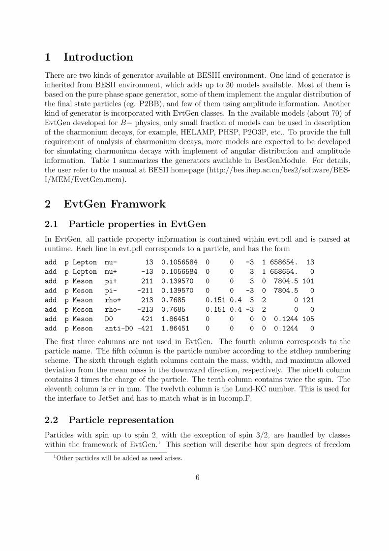
The first three columns are not used in EvtGen. The fourth column corresponds to theparticle name. The fifth column is the particle number according to the stdhep numberingscheme. The sixth through eighth columns contain the mass, width, and maximum alloweddeviation from the mean mass in the downward direction, respectively. The nineth columncontains 3 times the charge of the particle. The tenth column contains twice the spin. Theeleventh column is cτ in mm. The twelvth column is the Lund-KC number. This is used forthe interface to JetSet and has to match what is in lucomp.F.

2.2 Particle representation

Particles with spin up to spin 2, with the exception of spin 3/2, are handled by classeswithin the framework of EvtGen.1 This section will describe how spin degrees of freedom

1Other particles will be added as need arises.

6

Table 1: Generators available in BesGenModule.Name DescriptionBhagen radiative Bhabha scattering up to α3 order of QEDDdgen ψ

′′ → DD̄Ddprod DD̄ pair with the correct angular distribution.Dsdgen e+e− → D∗DDssgen e+e− → D∗D̄∗

Epscat Bhabha scattering with angular distribution.Fff e+e− → qq̄ →hadron according to Field-Feynman Fragmentation model.Ffgen e+e− → D+

s D−s

Fixpt To use for testing, debugging, checking efficiencies, to generatespecific particle in given distribution with fixed momentum.

Fsfgen ψ → F ∗F2, F∗ → γF1 decay type

Gamma2 double photon process for e+e− → P−P+Q−Q+,with P,Q = e, µ, τ , or quarks.

Howl pure phase spaceKk2f e+e− → γ → l+l− or qq̄Koralbe e+e− → τ+τ−, ref. CERN-Th-5885/90Kstark ψ → K∗K → KK̄πLund Lund model: e+e− → ψ, ψ(2S) → hadrons, e+e− → γ∗ → hadronsMugen e+e− → µ+µ−(γ), up to α3 order QED.P2bb ψ, ψ(2S) → BB̄ with angular distribution 1 + α cos2 θP2epem ψ → e+e− with angular distribution 1 + cos2 θP2mumu ψ → µµ with angular distribution 1 + cos2 θPpgen ψ(2S) exclusive decays, some with angular distribution information.Radee e+e− → e+e−γRadgg e+e− → γγγ, Ref. Nucl. Phys. B186(1981), 22Radmu e+e−µ+µ−

Rhopi ψ → 3π via ρπ with the angular distribution sin2 θSagerx ψ → γX, X → PP ,P=pseudoscalarTauprd ?Tester A simple 4-vector generatorTwogam 2γ process, similar to Gamma2V2llg V → l+l−γ up to α3 order QED

7

are represented, and will introduce the classes that represent particles in EvtGen. Table 2summarizes the different types of particles currently implemented.

Class name Rep. J States ExampleEvtScalarParticle 1 0 1 π, B0

EvtDiracParticle uα 1/2 2 e, τEvtNeutrinoParticle uα 1/2 1 νe

EvtVectorParticle εµ 1 3 ρ, J/ΨEvtPhotonParticle εµ 1 2 γEvtTensorParticle T µν 2 5 D∗

2, f2

Table 2: The different types of particles that supported by EvtGen. The spin 3/2, Rarita-Schwinger, representation has not yet been implemented.

In Table 2, uα represents a four component Dirac spinor, defined in the Pauli-Diracconvention for the gamma matrices, as discussed in Section 2.3.4. The EvtDiracParticleclass represents massive spin 1/2 particles that have two spin degrees of freedom. Neutrinosare also represented with a 4-component Dirac spinor by the EvtNeutrinoParticle class.Neutrinos are assumed to be massless and only left handed neutrinos and right handedanti-neutrinos are considered.

The complex 4-vector εµ is used to represent the spin degrees of freedom for spin 1particles. Massive spin 1 particles, represented by the EvtVectorParticle class, have threedegrees of freedom. The EvtPhotonParticle class represents massless spin 1 particles, whichhave only two (longitudinal) degrees of freedom.

Massive spin 2 particles are represented with a complex symmetric rank 2 tensor and areimplemented in the EvtTensorParticle class.

For each particle initialized in EvtGen, a set of basis states is created, where the numberof basis states is the same as the number of spin degrees of freedom. These basis states canbe accessed through the EvtParticle class in either the particle’s rest frame or in the parent’srest frame. For massless particles, only states in the parent’s rest frame are available. As anexample, consider the basis for a massive spin 1 particle in it’s own rest frame

εµ1 = (0, 1, 0, 0), (1)

εµ2 = (0, 0, 1, 0), (2)

εµ3 = (0, 0, 0, 1). (3)

Note that these basis vectors are mutually orthogonal, and normalized. That is,

gµνε∗µi εν

j = −δij. (4)

Further, they form a complete set∑

i

ε∗µi ενi = gµν − pµpν/m2, (5)

8

where gµν − pµpν/m2 is the propagator for an on-shell spin 1 particle.In order to write a new decay model, there is no reason to need to know the exact choice

of these basis states. The code needed to describe the amplitude for a decay process isindependent of these states, as long as they are complete, orthogonal and normalized.

2.3 Conventions

This section discusses the conventions we use for various physics quantities in the code.

2.3.1 Units

In EvtGen, c = 1, such that mass, energy and momentum are all measured in units of GeV.Similarly, time and space have units of mm.

2.3.2 Four-vectors

There are two types of four-vectors used in EvtGen, EvtVector4R and EvtVector4C, whichare real and complex respectively.

A four-vector is represented by pµ = (E, ~p). When a four-vector is used its componentsare always corresponding to raised indices. A contraction of two vectors p and k (p*k)automatically lowers the indices on k according to the metric g = diag(1,−1,−1,−1) sothat p*p is the mass squared of a particle with four-momentum p.

2.3.3 Tensors

We currently only support complex second rank tensors. As in the case of vectors, tensorsare always reperesented with all indices raised. The convention for the totaly antisymmetrictensor, εαβµν , is ε0123 = +1.

2.3.4 Dirac spinors

Dirac spinors are represented as a 4 component spinor in the Dirac-Pauli representation,with initial state fermions or final state anti-fermions.

2.3.5 Gamma matrices

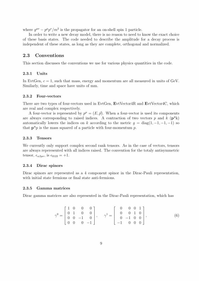
Dirac gamma matrices are also represented in the Dirac-Pauli representation, which has

γ0 =

1 0 0 00 1 0 00 0 −1 00 0 0 −1

, γ1 =

0 0 0 10 0 1 00 −1 0 0

−1 0 0 0

, (6)

9

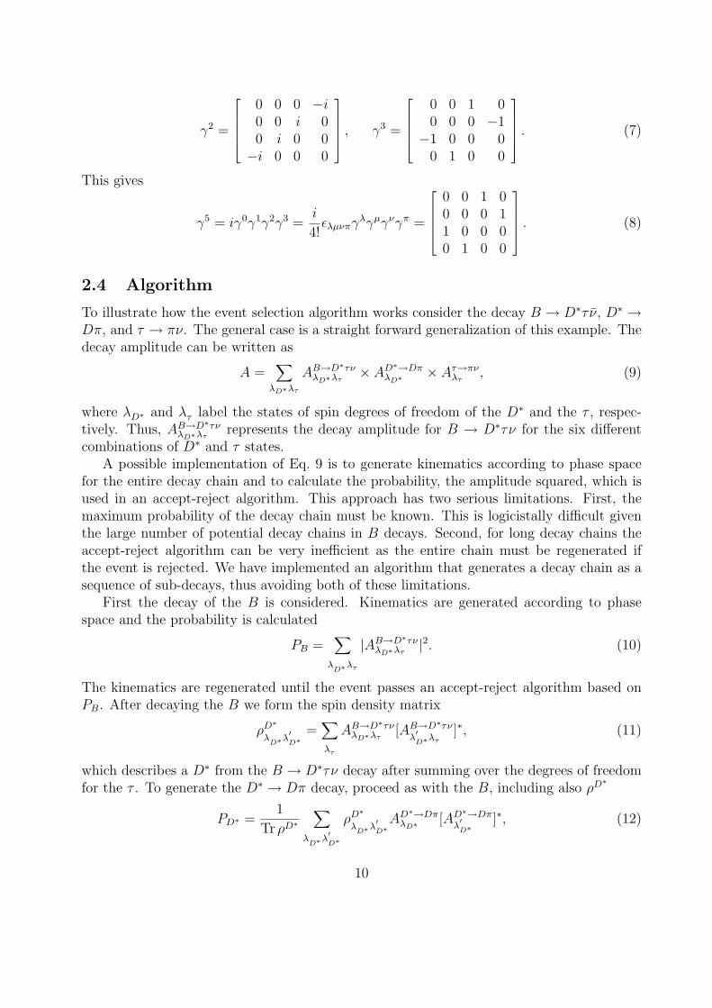
γ2 =

0 0 0 −i0 0 i 00 i 0 0−i 0 0 0

, γ3 =

0 0 1 00 0 0 −1

−1 0 0 00 1 0 0

. (7)

This gives

γ5 = iγ0γ1γ2γ3 =i

4!ελµνπγλγµγνγπ =

0 0 1 00 0 0 11 0 0 00 1 0 0

. (8)

2.4 Algorithm

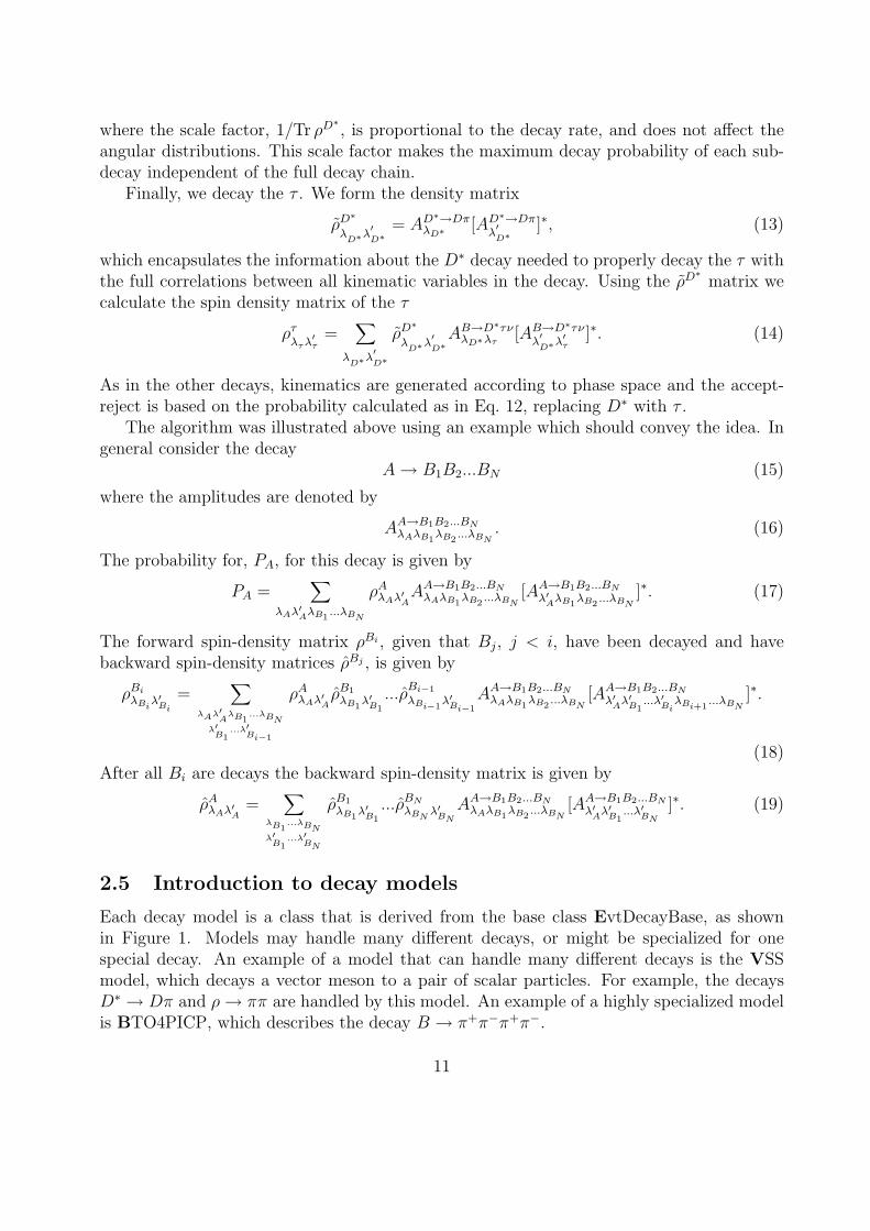
To illustrate how the event selection algorithm works consider the decay B → D∗τ ν̄, D∗ →Dπ, and τ → πν. The general case is a straight forward generalization of this example. Thedecay amplitude can be written as

A =∑

λD∗λτ

AB→D∗τνλD∗λτ

× AD∗→DπλD∗ × Aτ→πν

λτ, (9)

where λD∗ and λτ label the states of spin degrees of freedom of the D∗ and the τ , respec-tively. Thus, AB→D∗τν

λD∗λτrepresents the decay amplitude for B → D∗τν for the six different

combinations of D∗ and τ states.A possible implementation of Eq. 9 is to generate kinematics according to phase space

for the entire decay chain and to calculate the probability, the amplitude squared, which isused in an accept-reject algorithm. This approach has two serious limitations. First, themaximum probability of the decay chain must be known. This is logicistally difficult giventhe large number of potential decay chains in B decays. Second, for long decay chains theaccept-reject algorithm can be very inefficient as the entire chain must be regenerated ifthe event is rejected. We have implemented an algorithm that generates a decay chain as asequence of sub-decays, thus avoiding both of these limitations.

First the decay of the B is considered. Kinematics are generated according to phasespace and the probability is calculated

PB =∑

λD∗λτ

|AB→D∗τνλD∗λτ

|2. (10)

The kinematics are regenerated until the event passes an accept-reject algorithm based onPB. After decaying the B we form the spin density matrix

ρD∗

λD∗λ

′D∗

=∑

λτ


[AB→D∗τνλ′D∗λτ

]∗, (11)

which describes a D∗ from the B → D∗τν decay after summing over the degrees of freedomfor the τ . To generate the D∗ → Dπ decay, proceed as with the B, including also ρD∗

PD∗ =1

Tr ρD∗∑

λD∗λ

′D∗

ρD∗

λD∗λ

′D∗

AD∗→DπλD∗ [AD∗→Dπ

λ′D∗

]∗, (12)

10

where the scale factor, 1/Tr ρD∗ , is proportional to the decay rate, and does not affect theangular distributions. This scale factor makes the maximum decay probability of each sub-decay independent of the full decay chain.

Finally, we decay the τ . We form the density matrix

ρ̃D∗

λD∗λ

′D∗

= AD∗→DπλD∗ [AD∗→Dπ

λ′D∗

]∗, (13)

which encapsulates the information about the D∗ decay needed to properly decay the τ withthe full correlations between all kinematic variables in the decay. Using the ρ̃D∗ matrix wecalculate the spin density matrix of the τ

ρτλτ λ′τ

=∑

λD∗λ

′D∗

ρ̃D∗

λD∗λ

′D∗


[AB→D∗τνλ′D∗λ′τ

]∗. (14)

As in the other decays, kinematics are generated according to phase space and the accept-reject is based on the probability calculated as in Eq. 12, replacing D∗ with τ .

The algorithm was illustrated above using an example which should convey the idea. Ingeneral consider the decay

A → B1B2...BN (15)

where the amplitudes are denoted by

AA→B1B2...BNλAλB1

λB2...λBN

. (16)

The probability for, PA, for this decay is given by

PA =∑

λAλ′AλB1...λBN

ρAλAλ′A


λB2...λBN

[AA→B1B2...BN

λ′AλB1λB2

...λBN]∗. (17)

The forward spin-density matrix ρBi , given that Bj, j < i, have been decayed and havebackward spin-density matrices ρ̂Bj , is given by

ρBi

λBiλ′Bi

=∑

λAλ′A

λB1...λBN

λ′B1

...λ′Bi−1

ρAλAλ′A

ρ̂B1

λB1λ′B1

...ρ̂Bi−1

λBi−1λ′Bi−1


λB2...λBN

[AA→B1B2...BN

λ′Aλ′B1...λ′Bi

λBi+1...λBN

]∗.

(18)After all Bi are decays the backward spin-density matrix is given by

ρ̂AλAλ′A

=∑

λB1...λBN

λ′B1

...λ′BN

ρ̂B1

λB1λ′B1

...ρ̂BN

λBNλ′BN


λB2...λBN

[AA→B1B2...BN

λ′Aλ′B1...λ′BN

]∗. (19)

2.5 Introduction to decay models

Each decay model is a class that is derived from the base class EvtDecayBase, as shownin Figure 1. Models may handle many different decays, or might be specialized for onespecial decay. An example of a model that can handle many different decays is the VSSmodel, which decays a vector meson to a pair of scalar particles. For example, the decaysD∗ → Dπ and ρ → ππ are handled by this model. An example of a highly specialized modelis BTO4PICP, which describes the decay B → π+π−π+π−.

11

EvtDecayBase

EvtDecayAmp

EvtPHSP

EvtJetSet

EvtPi0Dalitz

EvtVSS

EvtISGW2

EvtDecayProb EvtDecayIncoherent

Figure 1: Diagram of the EvtDecayBase class and classes derived from it. EvtDecayAmp,EvtDecayTBaseProb, and EvtDecayIncoherent are templated classes that are used by mod-ules that compute the full decay amplitude, that compute the decay probability, and thosethat return unpolarized daughters, respectively.

12

2.6 Creating new decay models

To simplify the writing of decay models there are three different classes that are derived fromEvtDecayBase. These are EvtDecayAmp, EvtDecayProb, and EvtDecayIncoherent. Whenwriting decay models it is most convenient to derive from one of these classes. These classeshave slightly different interfaces depending on what information the decay model provides.Some models will provide the complete amplitude information where as other models mightprovide just a probability or a set of four-vectors. Models that don’t provide the full set ofamplitudes will of course not be able to simulate the complete angular distributions. Below,a short description is given to explain when you want to use each of these classes as the baseclass for your decay model.

• EvtDecayAmp allows you to specify the complete amplitudes and hence do a completesimulation of the angular distributions.

• EvtDecayProb allows you to calculate a probability for the decay. This probabilityis then used in the accept-reject method. Any spin information is lost, all producedparticles are unpolarized and uncorrelated.

• EvtDecayIncoherent just accepts the four vectors as generated. This is most usefulwhen interfacing to another generator, e.g. JetSet. Any spin information is lost, allproduced particles are unpolarized and uncorrelated.

2.7 Available base classes in EvtGen

• EvtAmp:This class keeps track of the amplitudes computed by the decay models. It providesmember functions to calculate spin-density matrices from the amplitudes.

• EvtCPU:This class contains some utilities that are useful for generating CP -violating decaysfrom the Υ(4S) system.

• EvtComplex:Using the implementation of complex numbers provided by the compiler has causedconstant problems with porting EvtGen to different platforms, as these implementa-tions do not generally conform to a uniform standard. Therefore, we have implementedthe EvtComplex class. This implemention is not complete.

• EvtConst:This class defines useful constants.

• EvtDecayBase:This class is the base class for decay models and contains the interface for the decaymodels to the framework.

13

• EvtDiraSpinor:The EvtDiracSpinor class encapsulates the properties of a Dirac spinor. It is used toreperesent spin 1/2 particles.

• EvtGammaMatrix:EvtGammaMatrix is a class for handling complex 4× 4 matrices.

• EvtGen:This class provides the interface to EvtGen for an external user.

• EvtGenKin:EvtGenKine contains tools for generating kinematics such as phase space distributions.

• EvtID:The class EvtId is used to identify particles in EvtGen.

• EvtKine:This class provides some utility functions for calculating kinematic quantities such asdecay angles.

• EvtLineShape:This class contains utilities for simulating line shapes of particles. Currently this classonly provides the trivial implementation of a non-relativistic Breit-Wigner shape.

• EvtModel:This class handles the registration of decay models.

• EvtPDL:The particle information read from the evt.pdl file can be accessed through memberfunctions of the EvtPDL class.

• EvtPHOTOS:Provides an interface to the PHOTOS package for generation of final state radiation.

• EvtPartProp:Class to represent the particle properties of a single particle. Used by EvtPDL to keepthe particle properties.

• EvtParticle:This is the base class for particles. It contains the common interface to particles suchas the four momentum particle number, list of daughters and parent etc.

• EvtParticleDecay:Stores information for one particle decay. This class is not used yet.

• EvtParticleDecayList:Stores the list of decays of one particle. This class is not used yet

14

• EvtParticleNum:Defines EvtID for all particles.

• EvtParser:Used by EvtDecayTable to read the decay table.

• EvtRandom:EvtRandom provides the interface for random numbers that are used inthe EvtGen package.

• EetReadDecay:This is a real mess! But it’s purpose is to read in the decay table.

• EvtReport:Utility to print out mesages from EvtGen.

• EvtResonance:The EvtResonance class allows one to handle resonances as a single structure.

• EvtSecondary:Allows EvtGen not to write secondary particles to StdHep.

• EvtSpinDensity:This class represents spin-density matrices of arbitrary dimensions. (Well, this is notquite true, at the moment it is limited to dimension 5 which is the number of degreesof freedom of a spin 2 particle.)

• EvtSpinType:Defines the folowing enum for the different particle types that EvtGen handles.

enum spintype { SCALAR,VECTOR,TENSOR,DIRAC,PHOTON,NEUTRINO,STRING };

• EvtStdHep:This class flattens out the EvtGen decay tree that is used internaly to represent theparticles and stores the particles in a structure that is parallel to StdHep.

• EvtString:This class is used by EvtGen to represent character strings.

• EvtSysTable:Variables that are defined using a “Define” statement in the decay table are stored inthis class.

• EvtTemplateDummy:This class was introduced just such that the EvtGen package made use of templates,this should be removed.

• EvtTensor3C:Complex rank 2 tensors in 3 dimensions.

15

• EvtTensor4C:This class encapsulates the properties of second rank complex tensors.

• EvtVector3C:Complex three-vectors.

• EvtVector3R:Real three-vectors.

• EvtVector4C:This is a class for reperesenting complex four-vectors.

• EvtVector4R:This is a class for representing real four vectors.

3 EvtGen developed at BESIII

3.1 Helicity amplitudes

In the models available in EvtGen, most of them are constructed in covariant amplitudeform. However, the partial wave ratios are not usually reported by experiments. For studyingthe particle polarization, the helicity amplitude can be measured. For combining experimen-tal information in the amplitude, we use the helicity amplitude form to describe the particledecays. For example, to consider the decay C → A + B, the initial particle, C, is assumedto be in the state |JM〉 and the final state, A + B, is |pJMλAλB〉. We will assume thatthe interaction U that causes this transition is invariant under rotation, but is otherwisearbitrary. The matrix element can be expressed by:

M = 〈pJMλAλB〉|U |JM〉. (20)

=

√2J + 1

4πD∗J

M,λA−λB(φ, θ,−φ)HλAλB

(21)

where the helicity amplitudes are defined by

HλAλB= 〈pJMλAλB|U |JM〉. (22)

For sequential decays, e.g. A → B + C, B → D + E, and C → F + G. The initialparticle, A, is in the state |J = JA m = λA〉. The amplitudes for the decay A → B + C isnow given by

AA→B+CλAλBλC

=

√2JA + 1

4πD∗JA

λA,λB−λC(φB, θB,−φB)HA

λBλC(23)

where θB and φB are the polar angles of particle B in the rest frame of particle A.Similarly, we can write the amplitude for the decay of particle B

AB→D+EλBλDλE

=

√2JB + 1

4πD∗JB

λB ,λD−λE(φD, θD,−φD)HB

λDλE. (24)

16

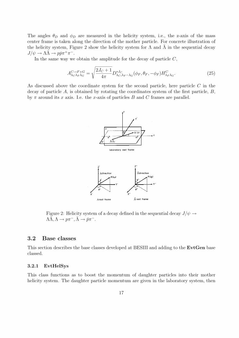
The angles θD and φD are measured in the helicity system, i.e., the z-axis of the masscenter frame is taken along the direction of the mother particle. For concrete illustration ofthe helicity system, Figure 2 show the helicity system for Λ and Λ̄ in the sequential decayJ/ψ → ΛΛ̄ → pp̄π+π−.

In the same way we obtain the amplitude for the decay of particle C,

AC→F+GλCλF λG

=

√2JC + 1

4πD∗JC

λC ,λF−λG(φF , θF ,−φF )HC

λF λG. (25)

As discussed above the coordinate system for the second particle, here particle C in thedecay of particle A, is obtained by rotating the coordinates system of the first particle, B,by π around its x axis. I.e. the x-axis of particles B and C frames are parallel.

Figure 2: Helicity system of a decay defined in the sequential decay J/ψ →ΛΛ̄, Λ → pπ−, Λ̄ → p̄π−.

3.2 Base classes

This section describes the base classes developed at BESIII and adding to the EvtGen baseclassed.

3.2.1 EvtHelSys

This class functions as to boost the momentum of daughter particles into their motherhelicity system. The daughter particle momentum are given in the laboratory system, then

17

boosted in their mother CM system and performing a rotation to the helicity system. Thisclass contains member functions needed for this helicity transformation.

• friend double djmn(int j, int m, int n, double theta);To define Wigner d function. The j, m and n are defined differently from the classEvtdFunction, such that djmn(1, 0, 0, theta) = cos(theta).

• friend EvtComplex Djmn(int j, int m, int n, double phi,double theta,doublegamma);To define big D function based on the Wigner d function djmn(j,m,n,theta).

• EvtVector4R Helrotate(EvtVector4R p1, double phi, double theta);To rotate the 3-vector momentum of ~p1 to the direction ~p(|~p|, θ, φ).

• double getHelAng(int i);To get the angle (θ, φ) of the daughter momentum in the helicity system via thedefinition θ =getHelAng(1), φ =getHelAng(2) and |~p| =getHelAng(0).

4 Decay models for charmonium physics

This section lists the different decay models that has been implemented in EvtGen only forcharmonium physics developed at BESIII. The models available in EvtGen V00-11-07 arenot include in this section, and they are summarized in Table 3. The user should refer tothe manual of EvtGen.

4.1 JPIPI

Author:Rong-Gang PingUsage:BrFr J/psi pi+ pi- JPIPI;

Explanation:

This model is constructed for the decay ψ′ → J/ψππ, which is similar to the model VVPIPIin EvtGen, but the amplitude is a little different. In the model VVPIPI, the amplitude forthe mass of the ππ system is given by A ∝ (m2

ππ−4m2π). In the model JPIPI, the amplitude is

constructed by the chiral effective Lagrangian as AΛM ∝ [g(m2ππ−2m2

π)+2g1Eπ+Eπ− ]ε∗ψ(M)·εψ′(Λ), and the parameters are taken by fit to the experimental mass spectrum of two pions[1], g = 0.3± 0.02, g1 = −0.11± 0.01.

Example:

Decay psi(2S)1.000 J/psi pi+ pi- JPIPI;Enddecay

18

Table 3: Available decay models in EvtGen are suitable for cha-monium decays, where S,P,T, L denote scalar, pseudoscalar ten-sor and lepton, respectively.

DECAY MODEL DECAY MODELHELAMP Any two body decayOMEGA DALITZ ω → 3πPARTWAVE Any two body decayPHSP Any decayPTO3P P→ 3P: ηc → ηππSINGLE Any decaySLN Any decaySTS S→TSSVP HELAMP S→VPSVS S→VSSVV HELAMP S→VVTAULNUNU τ → eνeντ

TAUSCALARNU τ → S + ντ

TAUVECTORNU τ → V + ντ

TSS T→SSTVS PWAVE T→VS only p-waveVECTORISR e+e− → V γVLL V→LL:J/ψ → e+e−, µ+µ−, ...VSP PWAVE v→SP, only p-waveVSS V→SS:J/ψ → KK̄, ...VVPIPI V→ Vππ:ψ′ → J/ψππ, ...VVS PWAVE V→VS:a0

0, J/ψ → ρπ, ...

19

Notes:

4.2 AngSam

Author:Rong-Gang PingUsage:BrFr D1 D2 AngSam Parameter;

Explanation:

This model is constructed for the two body decay A → B + C with the daughter particle Ataking the angular distribution dΓ

d cos θ∝ (1 + α cos2 θ) with a parameter α in the laboratory

frame. The α could be negative or positive real numbers.

Example:

ψ′ → pp̄ with the angular parameter α = 0.5:Decay psi(2S)1.000 p+ anti-p- AngSam 0.5;Enddecay

Notes:

Since this model is only based on angular distribution information in the laboratory frame,it is not suitable to the sequential decays. It is only for the decay e+e− → A → B + C.

4.3 P2GC0

Author:Rong-Gang PingUsage:BrFr gamma chi c0 P2GC0;

Explanation:

This model is constructed for the decay ψ′ → γχc0. The amplitude is constructed in thehelicity amplitude given by M ∝ D1∗

m,λ(θ, φ)Aλ, where the m and the λ are the helicity valueof ψ′ and photon, respectively. For consideration of CP invariance, the helicity amplitudessatisfy the relation A−λ = Aλ. The angular distribution of the outgoing photon takes theform:

d|M |2d cos θ

∝ (1 + cos2 θ).

Example:

ψ(2S) → γχc0:

20

Decay psi(2S)1.000 gamma chi c0 P2GC0;Enddecay

Notes:

4.4 P2GC1


Explanation:


m,λ1−λ2(θ, φ)Aλ1,λ2 , where m,λ1 and λ2 are the helicity

values of the ψ′, γ and χc1, respectively. For consideration of CP invariance, the helicityamplitudes satisfy the relation A−λ1,−λ2 = −Aλ1,λ2 . The angular distribution of the outgoing

photon takes the form d|M |2d cos θ

∝ (1+α cos2 θ), where α = |A1,0|2−2|A1,1|2|A1,0|2+2|A1,1|2 . It is believed that the

E1 dominates this process with α = −1/3 [2], so we take A11 = A10 = 1.

Example:

ψ(2S) → γχc1:Decay psi(2S)1.000 gamma chi c1 P2GC1;Enddecay

Notes:

4.5 P2GC2


Explanation:



values of the ψ′, γ and χc2, respectively. For consideration of CP invariance, the helicityamplitudes satisfy the relation A−λ1,−λ2 = Aλ1,λ2 . The angular distribution of the outgoing

21

photon takes the form d|M |2d cos θ

∝ (1 + α cos2 θ), where α = |A1,0|2−2|A1,1|2+|A1,2|2|A1,0|2+2|A1,1|2+|A1,2|2 . Theoretically,

it is believed that if the E1 dominates this process, the parameter α = 1/13 [2]. Experimen-tally, the the helicity amplitudes have been measured by BESII [3], and they are taken asA1,1/A1,0 = 2.08, A1,2/A1,0 = 3.03.

Example:

ψ(2S) → γχc2:Decay psi(2S)1.000 gamma chi c2 P2GC2;Enddecay

Notes:

4.6 AV2GV

Author:Rong-Gang PingUsage:BrFr gamma J/psi AV2GV;

Explanation:

This model is constructed for the decay χc1 → γJ/ψ. The amplitude is constructed in thehelicity amplitude given by M ∝ D1∗


values of the χc1, γ and J/ψ, respectively. For consideration of CP invariance and angulardistribution, the helicity amplitudes satisfy the relation A−λ1,−λ2 = −Aλ1,λ2 . There are twotwo independent amplitudes A1,1 and A10. Theoretically, it is believed that if the E1 dom-inates this process, the polar angle of the photon relative the photon (γ1) direction in the

decay e+e− → ψ′ → γ1χc1 → γ1γJ/ψ takes the form d|M |2d cos θ

∝ 5 + cos2 θ [4]. We use thisinformation to fix the ratio |A1,0/A1,1|.Example:

χc1 → γJ/ψ:Decay chi c11.000 gamma J/psi AV2GV;Enddecay

Notes:

22

4.7 T2GV

Author:Rong-Gang PingUsage:BrFr gamma J/psi T2GV;

Explanation:

This model is constructed for the decay χc2 → γJ/ψ. Since no experimental informationabout the helicity amplitudes for this decay is available. Theoretically, it is believed thatif the E1 dominates this process, the polar angle of the photon relative the photon (γ1)

direction in the decay e+e− → ψ′ → γ1χc2 → γ1γJ/ψ takes the form d|M |2d cos θ

∝ 73 + 21 cos2 θ[4]. The model is coded with pure phase space constrained with this angular information.

Example:

χc2 → γJ/ψ:Decay chi c11.000 gamma J/psi T2GV;Enddecay

Notes:

4.8 J2BB1

Author:Cai-Ying Pang, Rong-Gang PingUsage:BrFr p+ anti-p- J2BB1 parameter;

Explanation:

This model is constructed for the decay ψ′ and J/ψ decays into octet baryon and anti-baryonpair. The amplitude is constructed in the helicity amplitude given by M ∝ D1∗

m,λ1−λ2(θ, φ)Aλ1,λ2 ,

where m,λ1 and λ2 are the helicity values of the J/ψ, baryon and anti-baryon, respectively.For consideration of CP invariance, the helicity amplitudes satisfy the relation A−λ1,−λ2 =

Aλ1,λ2 . The angular distribution of the outgoing proton takes the form d|M |2d cos θ

∝ (1+α cos2 θ)

with α = |A+−|2−2|A++|2|A+−|2+2|A++|2 . The angular distribution parameters are the user input. Experimen-

tally, they are give as shown in Table 4. If users do not provide parameter, the default angular

distribution parameter are calculated in terms of Carimalo formula [5] α = (1+u)2−u(1+6u)2

(1+u)2+u(1+6u)2

with u = mB/M , where mB and M are the mass of the baryon and the mother particle,respectively.

Example:

J/ψ → pp̄:

23

Table 4: Angular distribution parameter α for J/ψ → BB̄decays. They are assumed to be the form of dN/d cos θ ∝1 + α cos2 θ.

Calculated value of αDecay mode Measured value of α Ref. [5]J/ψ → pp̄ 0.68± 0.06[6] 0.69J/ψ → ΛΛ̄ 0.65± 0.11[7] 0.51J/ψ → Σ0Σ̄0 −0.24± 0.20[7] 0.43J/ψ → Ξ−Ξ̄+ −0.13± 0.59[8] 0.27ψ′ → pp̄ 0.67± 0.16[9] 0.80

Decay J/psi1.000 p+ anti-p- J2BB1 0.68;Enddecay

Notes:

4.9 J2BB2


Explanation:

This model is constructed for the decay ψ′ and J/ψ decays into decuplet baryon andanti-baryon pair. The amplitude is constructed in the helicity amplitude given by M ∝D1∗

m,λ1−λ2(θ, φ)Aλ1,λ2 , where m,λ1 and λ2 are the helicity values of the J/ψ, baryon and anti-

baryon, respectively. For consideration of CP invariance, the helicity amplitudes satisfy therelation A−λ1,−λ2 = Aλ1,λ2 . The angular distribution of the outgoing photon takes the form

d|M |2d cos θ

∝ (1 + α cos2 θ) with α =|A 1

2−12|2+2|A 1

232|2−2(|A 1

212|2+|A 3

232|2)

|A 12−

12|2+2|A 1

232|2+2(|A 1

212|2+|A 3

232|2)

. The angular distribution

parameters are the user input. .

Example:

J/ψ → ∆++∆̄−−:Decay J/psi1.000 Delta++ anti-Delta– J2BB2 0.68;Enddecay

24

Notes:

4.10 J2BB3


Explanation:

This model is constructed for the decay ψ′ and J/ψ decays into decuplet baryon plusoctet anti-baryon pair. The amplitude is constructed in the helicity amplitude given byM ∝ D1∗

m,λ1−λ2(θ, φ)Aλ1,λ2 , where m,λ1 and λ2 are the helicity values of the J/ψ, baryon

and anti-baryon, respectively. For consideration of CP invariance, the helicity amplitudessatisfy the relation A−λ1,−λ2 = Aλ1,λ2 . The angular distribution of the outgoing photon takes

the form d|M |2d cos θ

∝ (1 + α cos2 θ) with α =2|A 1

212|2+|A 1

2−12|2+|A 1

232|2

−2|A 12

12|2+|A 1

2−12|2+|A 1

232|2 . The angular distribution

parameters are the user input.

Example:

J/ψ → Σ+Σ̄∗−:Decay J/psi1.000 Sigma+ anti-Sigma*- J2BB3 0.68;Enddecay

Notes:

4.11 DIY

Author:Rong-Gang PingUsage:BrFr daughter 1 daughter 2... DIY;

Explanation:

The model Doing It Yourself (DIY) is created for user to generate event by supplying de-cay amplitude. The DIY model is useful for the user to generate event using partial waveanalysis results, or implementing coherent effects in decays, or parameterizing the physicalquantities in amplitude. The DIY generates events according the decay mode specified byuser with pure phase space and passing the four-vector momentum to the amplitude andcalculate the decay amplitude. The maximal value of the amplitude is singled out in 20,000events. Then it uses the reject-accepted sampling method to generate event. There are two

25

kinds of reference frames available to get the momentum of the final states. One is the centermass (CM) system of the mother particle and another is the helicity system with the z-axisis parallel to the outgoing direction of the mother particle in laboratory system. The userprovides amplitude via a class:

double EvtDIY::AmplitudeSquare(){ };

For example, a user defines an amplitude class for the decay J/ψ → ρπ → 3π as:

class rhopi{public:rhopi(EvtVector4R pd1, EvtVector4R pd2,EvtVector4R pd3){pd[0]=pd1;pd[1]=pd2;pd[2]=pd3;

}double amps( ); //calculate amplitudeprivate:EvtVector4R pd[2];}

///************* amplitude by userdouble EvtDIY::AmplitudeSquare(){EvtVector4R dp1=GetDaugMomLab(0);EvtVector4R dp2=GetDaugMomLab(1),dp3=GetDaugMomLab(2);rhopi Jpsi2rhopi(dp1,dp2,dp3);return Jpsi2rhopi.amps();}

Example:

Decay J/psi1.000 pi+ pi- pi0 DIY;Enddecay

Notes:

5 Test of Model

5.1 JPIPI

The model JPIPI is tested with the following decay table:Decay psi(2S)1.000 J/psi pi+ pi- JPIPI;

26

EnddecayEnd

(GeV)ππm0.3 0.35 0.4 0.45 0.5 0.55 0.6

EV

EN

TS

0

1000

2000

3000

4000

5000

6000

7000

8000

9000

ψ J/ππ→(2S)ψ

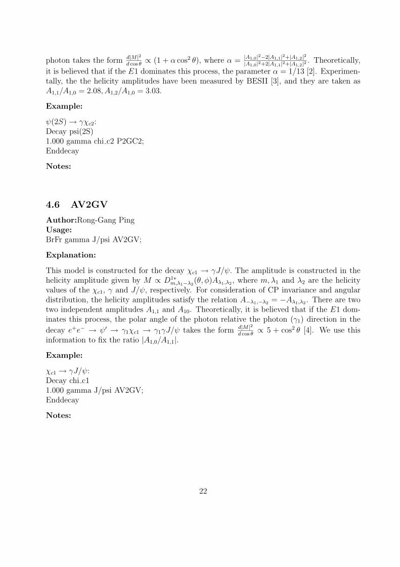
Figure 3: The comparison of the mass distribution of mππ in the ψ′ →J/ψππ between the model VVPIPI (error bar) and JPIPI (histogram)

5.2 AngSam

The model AngSam is tested by the decay J/ψ → pp̄ with the following decay table:Decay J/psi1.000 p+ anti-p- AngSam 0.67;EnddecayEnd

5.3 P2GC0

The model P2GC0 is tested by the decay ψ′ → γχc0 with the following decay table:Decay psi(2S)1.000 gamma chi c0 P2GC0;EnddecayEnd

5.4 P2GC1

The model P2GC1 is tested by the decay ψ′ → γχc0 with the following decay table:Decay psi(2S)

27

)pθcos(-1 -0.8 -0.6 -0.4 -0.2 -0 0.2 0.4 0.6 0.8 1

EV

EN

TS

400

450

500

550

600

650

Figure 4: The test of the model AngSam with the decay J/ψ → pp̄ byassuming the angular distribution dΓ/d cos θ ∝ (1 + α cos2 θ). The inputangular distribution parameter α = 0.5, the fit result is α′ = 0.53± 0.02.

)γθcos(-1 -0.8 -0.6 -0.4 -0.2 -0 0.2 0.4 0.6 0.8 1

EV

EN

TS

350

400

450

500

550

600

650

700

750

Figure 5: The model P2GC0 is tested by the angular distribution of pho-ton in the ψ′ → γχc0. The input angular distribution parameter α = 1,the fit result is α′ = 1.02± 0.02.

28

1.000 gamma chi c1 P2GC1;EnddecayEnd

)γθcos(-1 -0.8 -0.6 -0.4 -0.2 -0 0.2 0.4 0.6 0.8 1

EV

EN

TS

400

450

500

550

600

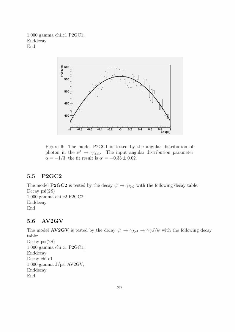
Figure 6: The model P2GC1 is tested by the angular distribution ofphoton in the ψ′ → γχc1. The input angular distribution parameterα = −1/3, the fit result is α′ = −0.33± 0.02.

5.5 P2GC2

The model P2GC2 is tested by the decay ψ′ → γχc2 with the following decay table:Decay psi(2S)1.000 gamma chi c2 P2GC2;EnddecayEnd

5.6 AV2GV

The model AV2GV is tested by the decay ψ′ → γχc1 → γγJ/ψ with the following decaytable:Decay psi(2S)1.000 gamma chi c1 P2GC1;EnddecayDecay chi c11.000 gamma J/psi AV2GV;EnddecayEnd

29

)γθcos(-1 -0.8 -0.6 -0.4 -0.2 -0 0.2 0.4 0.6 0.8 1

EV

EN

TS

440

460

480

500

520

540

Figure 7: The model P2GC2 is tested by the angular distribution of pho-ton in the ψ′ → γχc2. The input angular distribution parameter α = 1/13,the fit result is α′ = 0.057± 0.015.

)γγθcos(-1 -0.8 -0.6 -0.4 -0.2 -0 0.2 0.4 0.6 0.8 1

EV

EN

TS

380

400

420

440

460

480

500

520

540

560

580

Figure 8: The model AV2GV is tested by observing the angular distribu-tion of the photon in the χc1 → γJ/ψ with the reference of the photo di-rection in ψ′ → γχc1. The input angular distribution parameter α = 1/5,the fit result is α′ = 0.21± 0.02.

30

5.7 T2GV

The model T2GV is tested by the decay ψ′ → γχc2 → γγJ/ψ with the following decaytable:Decay psi(2S)1.000 gamma chi c2 P2GC2;EnddecayDecay chi c21.000 gamma J/psi T2GV;EnddecayEnd

)γγθcos(-1 -0.8 -0.6 -0.4 -0.2 -0 0.2 0.4 0.6 0.8 1

EV

EN

TS

400

450

500

550

600

Figure 9: The model T2GV is tested by observing the angular distributionof the photon in the χc2 → γJ/ψ with the reference of the photo directionin ψ′ → γχc2. The theoretical angular distribution parameter is expectedto be α = 21/73 by adjusting the helicity amplitudes. The parameter isfixed to be α′ = 0.29± 0.02. at present version.

5.8 J2BB1

The model J2BB1 is tested by the decay ψ′ → pp̄ with the following decay table:Decay psi(2S)1.000 p+ anti-p- J2BB1 0.67;EnddecayEnd

31

)pθcos(-1 -0.8 -0.6 -0.4 -0.2 -0 0.2 0.4 0.6 0.8 1

EV

EN

TS

1600

1800

2000

2200

2400

2600

2800

Figure 10: The model J2BB1 is tested by the ψ′ → pp̄ with the inputparameter α = 0.67 and the simulated value is α = 0.67± 0.01.

5.9 DIY

The model DIY is tested by the decay J/ψ → ρ(770)π → π+(p1)π0(p2)π

−(p3) with thefollowing decay table:Decay J/psi1.000 pi+ pi- pi0 DIY;EnddecayEnd

This model needs the user to provide the amplitudes, which is constructed as helicityamplitudes:

Aρ+

j (M) =∑

λ=−1,1

F 1λ,0(r3)D

1∗M,λ(θ3, φ3)BWj(s12)R

j0,0(r

∗1)D

1∗λ,0(θ12, φ12) for ρ+(770),(26)

Aρ−j (M) =

∑

λ=−1,1

F 1λ,0(r1)D


j0,0(r

∗2)D

1∗λ,0(θ23, φ23) for ρ−(770),(27)

Aρ0

j (M) =∑

λ=−1,1

F 1λ,0(r2)D


j0,0(r

∗3)D

1∗λ,0(θ13, φ13) for ρ0(770),(28)

where r∗1, r∗2 and r∗3 are respectively the momentum differences of the two pions’ in the CM

system of their mother particles ρ with quantum number JP = j−, and θ12 (φ12), θ23 (φ23)and θ13 (φ13) are the polar (azimuthal) angles of the momentum vector of π+, π0 and π− intheir mother particle CM system. BWj(s) denotes the Breit-Wigner of the ρ(j−) resonancewith a CM energy

√s. To consider the parity conservation for J/ψ(1−) → ρ(j−)π(0−), it

leads to F 100 = 0, thus the sum in the above equations runs over λ = ±1.

32

The helicity-coupling amplitudes F 1µ,ν and Rj

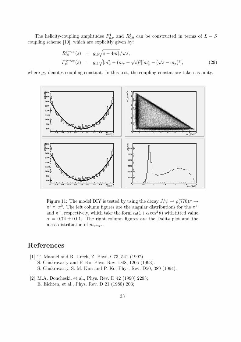
0,0 can be constructed in terms of L − Scoupling scheme [10], which are explicitly given by:

Rρ→ππ00 (s) = g10

√s− 4m2

π/√

s,

Fψ→ρπ10 (s) = g11

√[m2

ψ − (mπ +√

s)2][m2ψ − (

√s−mπ)2], (29)

where gls denotes coupling constant. In this test, the coupling constat are taken as unity.

)+π

θcos(-1 -0.8 -0.6 -0.4 -0.2 -0 0.2 0.4 0.6 0.8 1

EV

EN

TS

800

900

1000

1100

1200

1300

1400

1500

1600

)2(GeV2-π+πm

0 1 2 3 4 5 6 7 8 9

)2(G

eV2

0π

+π

m

0

1

2

3

4

5

6

7

8

9

)-πθcos(

-1 -0.8 -0.6 -0.4 -0.2 -0 0.2 0.4 0.6 0.8 1

EV

EN

TS

800

900

1000

1100

1200

1300

1400

1500

1600

(GeV)-π+πm0 0.5 1 1.5 2 2.5 3

EV

EN

TS

0

1000

2000

3000

4000

5000

6000

Figure 11: The model DIY is tested by using the decay J/ψ → ρ(770)π →π+π−π0. The left column figures are the angular distributions for the π+

and π−, respectively, which take the form c0(1+α cos2 θ) with fitted valueα = 0.74 ± 0.01. The right column figures are the Dalitz plot and themass distribution of mπ+π− .

References

[1] T. Mannel and R. Urech, Z. Phys. C73, 541 (1997).S. Chakravarty and P. Ko, Phys. Rev. D48, 1205 (1993).S. Chakravarty, S. M. Kim and P. Ko, Phys. Rev. D50, 389 (1994).

[2] M.A. Doncheski, et al., Phys. Rev. D 42 (1990) 2293;E. Eichten, et al., Phys. Rev. D 21 (1980) 203;

33

K.J. Sebastian, Phys.Rev. D 26 (1982) 2295;G. Hardekopf and J. Sucher, Phys. Rev. D 25 (1982) 2938; R. McClary and N. Byers,Phys. Rev. D 28 (1983) 1692;P. Moxhay and J.L. Rosner, Phys. Rev. D 28 (1983) 1132.

[3] M. Ablikim, et al., BES collaboration, Phys. Rev. D70 092004 (2004).

[4] Gabriel Karl, Sydney Meshkov and Jonathan L. Rosner, Phys. Rev. D 13, 1203 (1976).Lowell S. Brown and Robert N. Cahn, Phys. Rev. D 12, 2161 (1975).

[5] C. Carimalo, Int.J.Mod.Phys.A2:249,1987.

[6] BES Collaboration, J.Z. Bai, et.al., Phys. Lett. B 591 (2004) 42 .

[7] BES Collaboration, M.Ablikim, et.al., Phys. Lett. B 632 (2006) 181 .

[8] M. W. Eaton, et.al. Phys. Rev. D 29 (1984) 804 .

[9] Fermilab E835 Collaboration, A. Buzzo,

[10] Ping Rong-Gang, Li Gang and Wang Zheng, Comm. Theor. Phys.,

34

Index

algorithm, 10amplitude, 6

evt.pdl, 6

neutrino, 6

particle properties, 6photon, 6

representation, 6

scalar particle, 6spin, 6spin 1/2 particle, 6

tensor particle, 6

vector particle, 6

35

Acknowledgement:

This project is partially supported by Li HaiBo. We thank He Kang Lin, Li Hao Bo andLi WeiDong for close collaboration in model coding. We also thank BESIII collaboration forfinancial support to doing this project, we also thank many Chinese theoretical physicistsfor useful discussion on the model construction.

36

Monte Carlo Generators for Tau-Charm-Physics at...

Documents

Transcript of Monte Carlo Generators for Tau-Charm-Physics at...