Monopolistic Competition and OptimumProduct Diversity

B>'AviNASH K. DixiT AND J O S E P H E . STIGLITZ*

The basic issue concerning production inwelfare economics is whether a market solu-tion will yield the socially optimum kindsand quantities of commodities. It is wellknown that problems can arise for threebroad reasons: distributive justice; externaleffects; and scale economies. This paper isconcerned with the last of these.

The basic principle is easily stated.' Acommodity should be produced if the costscan be covered by the sum of revenues anda properly defined measure of consumer'ssurplus. The optimum amount is thenfound by equating the demand price and themarginal cost. Such an optimum can berealized in a market if perfectly discrim-inatory pricing is possible. Otherwise weface conflicting problems. A competitivemarket fuHilling the marginal conditionwouldbe unsustainable because total profitswould be negative. An element of monopolywould allow positive profits, but wouldviolate the marginal condition.^ Thus weexpect a market solution to be suboptimal.However, a much more precise structuremust be put on the problem if we are tounderstand the nature ofthe bias involved.

It is useful to think ofthe question as oneof quantity versus diversity. With scaleeconomies, resources can be saved by pro-ducing fewer goods and larger quantities ofeach. However, this leaves less variety,which entails some welfare loss. It is easyand probably not too unrealistic to modelscale economies by supposing that eaeh

* Professors of economics, University of Warwickand Stanford University, respectively. Stiglitz's re-search was supported in pan by NSF Grant SOC74-22182 at the Institute for Mathematical Studies in theSociai Sciences, Stanford. We are indebted to MichaelSpence, to a referee, and the managing editor for com-ments and suggestions on earlier drafts,

'Sec also the exposition by Michael Spence.A simple exposition is given by Peter Diamond and

Daniel McFadden.

potential commodity involves some fixedset-up cost and has a constant marginalcost. Modeling the desirability of varietyhas been thought to be difficult, and severalindirect approaches have been adopted.The Hotelling spatial model. Lancaster'sproduct characteristics approach, and themean-variance portfolio selection modelhave all been put to use.^ These lead to re-sults involving transport costs or correla-tions among commodities or securities, andare hard to interpret in general terms. Wetherefore take a direct route, noting that theconvexity of indifference surfaces of a con-ventional utility function defined over thequantities of all potential commodities al-ready embodies the desirability of variety.Thus, a consumer who is indifferent be-tween the quantities (1,0) and (0,1) of twocommodities prefers the mix (1/2,1/2) toeither extreme. The advantage of this viewis that the results involve the familiar own-and cross-elasticities of demand functions,and are therefore easier to comprehend.

There is one case of particular interest onwhich we concentrate. This is where poten-tial commodities in a group or sector or in-dustry are good substitutes among them-selves, but poor substitutes for the othercommodities in the economy. Then we areled to examining the market solution in re-lation to an optimum, both as regardsbiases within the group, and between thegroup and the rest of the economy. We ex-pect the answer to depend on the intra- andintersector elasticities of substitution. Todemonstrate the point as simply as possible,we shall aggregate the rest of the economyinto one good labeled 0, chosen as thenumeraire. The economy's endowment of itis normalized at unity; it can be thought ofas the time at the disposal of the consumers.

•'Sec the articles by Harold Hoiclling, NicholasStern, Kelvin Lancaster, and Stiglilz.

297

298 THE AMERICAN ECONOMIC REVIEW JUNE 1977

The potential range of related products islabeled 1,2.3 Writing the amounts ofthe various commodities as Vo and .V = (x,.Xi, Xi . . . , we assume a separable utilityfunction with convex indifference surfaces:

0) U -

In Sections I and II we simplify furtherby assuming that K is a symmetric function,and that all commodities in the group haveequal fixed and marginal costs. Then theactual labels given tu commodities are im-material, even though the total number nbeing produced is relevant. We can thuslabel these commodities 1,2 n. wherethe potential products (« + 1), (« + 2). . . .are not being produced. This is a restrictiveassumption, for in such problems we oftenhave a natural asymmetry owing to grad-uated physical differences in commodities,with a pair close together being bettermutual substitutes than a pair farther apart.However, even the symmetric case yieldssome interesting results. In Section III. weconsider some aspects of asymmetry.

We also assume that all commoditieshave unit income elasticities. This differsfrom a similar recent formulation byMichael Spencc, who assumes U linear inXo, so that the industry is amenable topartial equilibrium analysis. Our approachallows a better treatment ofthe interscctoralsubstitution, but the other results are verysimilar to those of Spence.

We consider two special cases of (1). InSection I, V is given a CES form, but U isallowed to be arbitrary. In Section II. U istaken to be Cobb-Douglas. but V has amore general additive form. Thus the for-mer allows more general intersector rela-tions, and the latter more general intra-sector substitution, highlighting differentresults.

Income distribution problems are ne-glected. Thus U can be regarded as repre-senting Samuelsonian social indifferencecurves, or (assuming the appropriate aggre-gation conditions to be fulfilled) as a mul-tiple of a representative consumer's utility.Product diversity can then be interpretedeither as different consumers using different

varieties, or as diversification on the partof each consumer.

[. Constant-Elasticity Case

A. Demand Functions

The utility function in this section is

(2) u =

For concavity, we need p < \. Further,since we want to allow a situation whereseveral of the Xj are zero, we need p > 0. Wealso assume U homothetic in its arguments.

The budget constraint is

(3)

where Pi are prices of the goods being pro-duced, and / is income in terms of thenumeraire, i.e., the endowment which hasbeen set at 1 plus the profits of the firmsdistributed to the consumers, or minus thelump sum deductions to cover the losses, asthe case may be.

In this case, a two-stage budgeting pro-cedure is valid.'' Thus we define dual quan-tity and price indices

(4) > • = q = .-\/ti

where /!i = (I - p)/p, which is positive since0 < p < 1. Then it can be shown^ that in thefirst stage.

(5) y - = /{I

for a function s which depends on the formof U. Writing (T{q) for the elasticity of sub-stitution between XQ and V, we define ffiq) asthe elasticity ofthe function .v. i.e.. qs'{q)lsiq). Then we find

(6)

butceed 1.

\\

can be negative as o{q) can ex-

ScL- p. 21 of John Green.These details and several others arc omitted to save

space, but can be found in the working paper by theauthors, cited in the references.

VOL 67 NO. 3 DtXIT AND STIGLITZ: PRODUCT DIVERSITY 299

Turning to the second stage ofthe prob-lem, it is easy to show that for each /,

(7) X, - y

where v is defined by (4). Consider the effectof a change in /?, alone. This affects x, di-rectly, and also through q: thence through vas well. Now from (4) we have the elasticity

^ log Pi \Pil

So long as the prices of the products in thegroup are not of different orders of mag-nitude, this is of the order ( l /«). We shallassume that n is reasonably large, and ac-cordingly neglect the effect of each p, on q;thus the indirect effects on x,. This leaves uswith the elasticity

dlogx, - 1 -(1 + (i)(9)

0 log Pi (1 - p)

In the Chamberlinian terminology, this isthe elasticity of the dd curve, i.e., the curverelating the demand for each product typeto its own price with all other prices heldconstant.

In our large group case, we also see thatfor / ^ j . the cross elasticity c* log xjb log p,is negligible. However, if all prices in thegroup move together, the individually smalleffects add to a significant amount. Thiscorresponds to the Chamberlinian DDcurve. Consider a symmetric situationwhere x, = x and p, = p for all / from 1to n. We have

(10) = xny = xiq = pn~'^ = p

and then from (5) and (7),

(11) X =pn

The elasticity of this is easy to calculate; wefind

(12)f* log X

= - [I -

Then (6) shows that the DD curve slopes

downward. The conventional condition thatthe dd curve be more elastic is seen from (9)and (12) to be

(13) h, + Hq) > 0

Finally, we observe that for / # j .

(14)1/(1-

Thus 1/(1 - p) is the elasticity of substitu-tion between any two products within thegroup.

B. Market Equilibrium

It can be shown that each commodity isproduced by one firm. Each firm attemptsto maximize its profit, and entry occurs un-til the marginal firm can only just breakeven. Thus our market equilibrium is thefamiliar case of Chamberlinian monopolis-tic competition, where the question ofquantity versus diversity has often beenraised.*" Previous analyses have failed toconsider the desirability of variety in an ex-plicit form, and have neglected variousintra- and intersector interactions in de-mand. As a result, much vague presumptionthat such an equilibrium involves excessivediversity has built up at the back of theminds of many economists. Our analysiswill challenge several of these ideas.

The profit-maximization condition foreach firm acting on its own is the familiarequality of marginal revenue and marginalcost. Writing c for the common marginalcost, and noting that the elasticity of de-mand for each firm is (1 -I- 0)/0, we havefor each active firm:

= c1 +

Writing p^ for the common equilibriumprice for each variety being produced, wehave

(15) p, = f(l -h /3) = -^P

^Scc Edwin Chamberlin, Nicholas Kaldor. andRobtrl Bishop.

300 THE AMERICAN ECONOMIC REVIEW JUNE 1977

The second condition for equilibrium isthat firms enter until the next potentialentrant would make a loss. If n is largeenough so that I is a small increment, wecan assume that the marginal firm is exactlybreaking even, i.e., (/)„ - c)x„ = a, where x„is obtained from the demand function and ais the fixed cost. With symmetry, this im-plies zero profit for all intramarginal firmsas well. Then / = 1, and using (11) and (15)we can write the condition so as to yield thenumber/7j. of active firms:

i\t.\ •''iPe^i'^) fl(16) = _

Equilibrium is unique provided sip^n''^)/p^n is a monotonic function of n. This re-lates to our earlier discussion about the twodemand curves. From (11) we see that thebehavior of s{pn~^)/pn as n increases tellsus how the demand curve DD for each firmshifts as the number of firms increases. It isnatural to assume that it shifts to the left,i.e., the function above decreases as n in-creases for each fixed p. The condition forthis in elasticity form is easily seen to be

1 + mq) > 0This is exactly the same as (13). the condi-tion for the ddcurvt to be more elastic thanthe/) /) curve, and we shall assume that itholds.

The condition can be violated if a(q) issufficiently higher than one. In this case, anincrease in n lowers q, and shifts demandtowards the monopolistic sector lo such anextent that the demand curve for each firmshifts to the right. However, this is ratherimplausible.

Conventional Chamberlinian analysis as-sumes a fixed demand curve for the groupas a whole. This amounts to assuming thatn-x is independent oi'n, i.e., that sipn -'^) isindependent of«. This will be so if ,t̂ = 0, or\f <T(q) = 1 lor ali q. The former is equiv-alent to assuming thai p = 1, when aliproducts in the group are perfect substi-tutes, i.e., diversity is not valued at all. Thatwould be contrary to the intent of the wholeanalysis. Thus, implicitly, conventionalanalysis assumes (T{q) = I. This gives a con-

stant budget share for the monopolisticallycompetitive sector. Note that in our para-metric formulation, this implies a unit-elastic DD curve, (17) holds, and so equi-librium is unique.

Finally, using (7), (11), and (16), we cancalculate the equilibrium output for eachactive firm:

(18) X. =(ic

We can also write an expression for thebudget share ofthe group as a whole:

where q^ = p^n;^

These will be useful for subsequent com-parisons.

C. Consirained Optimum

The next task is to compare the equi-librium with a social optimum. Witheconomies of scale, the first best or uncon-strained (really constrained only by tech-nology and resource availability) optimumrequires pricing below average cost, andtherefore lump sum transfers to firms tocover losses. The conceptual and practicaldifficulties of doing so are clearly formid-able. It would therefore appear that a moreappropriate notion of optimality is a con-strained one, where each firm must havenonnegative profits. This may be achievedby regulation, or by excise or franchisetaxes or subsidies. The important restrictionis that lump sum subsidies are not available.

We begin with such a constrained opti-mum. The aim is to choose «. /?,, and x, soas lo maximize utility, satisfying the de-mand functions and keeping the profit foreach firm nonnegative. The problem issomewhat simplified by the result that allactive firms should have the same outputlevels and prices, and should make exactlyzero profit. We omit ihe proof. Then we canset/ = 1, and use (5) to express utility as afunction of q alone. This is of course a de-creasing function. Thus the problem ofmaximizing u becomes that of minimizing</. i-t;.,

- 67 NO. 3 DIXIT AND STIOLITZ: PRODUCT DIVERSITY 301

mm pnn,p

(25) -{a + (1 + = 0

subject to

(20) = a

To solve this, we calculate the logarithmicmarginal rate of substitution along a leveleurve of the objective, the similar rate oftransformation along ihe constraint, andequate the two. This yields the condition

(21)p - c +

I +The second-order condition can be shownto hold, and (21) simplifies to yield the pricefor eaeh commodity produced in the con-strained optimum, p,. as

(22) /?, = r(l + (i)

Comparing (15) and (22), we see that theIwo solutions have the same price. Sincethey face the same break-even constraint,they have the same number of firms as well,and the values for all other variables can becalculated from these two. Thus we have arather surprising case where the monopo-listic competition equilibrium is identicalwith the optimum constrained by the lackof lump sum subsidies. Chamberlin oncesuggested that such an equilibrium was "asort of ideal"; our analysis shows when andin what sense this can be true.

D. Unconsl rained Optimum

These solutions can in turn be comparedto the unconstrained or first besi optimum.Considerations of convexity again establishthat al! active firms should produce thesame output. Thus we are to choose n firmseach producing output v in order to maxi-mize

(23) - n[a

where we have used the economy's resourcebalance condition and (10). The firsl-orderconditions are

From the firsl stage ofthe budgeting prob-lem, we know that q = UjL'o. Using (24)and (10), we find the price charged by eachactive firm in the unconstrained optimum,/?„, equal to marginal cost

(26) p. = c

This, of course, is no surprise. Also fromthe first-order conditions, we have

(27) X., =

Finally, wiih (26), each active firm covers itsvariable cost exactly. The lump sum trans-fers to firms then equal an. and therefore1 = \ - an, and

,v = (I -an)pn

The number of firms «„ is then defined by

(28) alii1 - an.

We can now compare these magnitudeswith the corresponding ones in the equilib-rium or Ihe constrained optimum. The mostremarkable result is that the output of eachactive firm is the same in the two situations.The fact that in a Chamberlinian equilib-rium each firm operates to the left of thepoint of minimum average cost has beenconventionally described by saying thatthere is excess capacity. However, whenvariety is desirable, i.e., when the differentproducts are not perfect substitutes, it is notin general optimum to push the output ofeach firm lo the point where all economiesof scale are exhausted.' We have shown inone case that is not an extreme one. that thefirst best optimum does not exploit econo-mies of scale beyond the extent achieved inthe equilibrium. We can then easily con-ceive of cases where the equilibrium exploitseconomies of scale too far from the point ofview of social optimality. Thus our resultsundermine the validity ofthe folklore of ex-cess capacity, from the poinl of view ofthe

(24) + 0 Djvid Siarrctl.

302 THE AMERICAN ECONOMIC REVIEW JUNE 1977

Kltil RH 1

unconstrained optimum as well as the con-strained one.

A direct comparison of the numbers offirms from (16) and (28) would be difficult,but an indirect argument turns out to besimple. It is clear that the unconstrainedoptimum has higher utility than the con-strained optimum. Also, the level of lumpsum income in it is less than that in the lat-ter. It must therefore be the case that

(29) < Qc =

Further, the difference must be largeenough that the budget constraint for XQand the quantity index y in the uncon-strained case must lie outside that in theconstrained case in the relevant region, asshown in Figure I. Let C be the constrainedoptimum. A the unconstrained optimum,and let B be the point where the line joiningthe origin to C meets the indifference curvein the unconstrained case. By homotheticitythe indifference curve at B is parallel to thatat C, so each ofthe moves from C to fi andfrom B io A increases the value of >". Sincethe value of x is the same in the two optima,we must have

(30) «, > n, = n.

Thus the unconstrained optimum actuallyallows more variety than the constrainedoptimum and the equilibrium; this isanother point contradicting the folklore onexcessive diversity.

Using (29) we can easily compare thebudget shares. In the notation we have beenusing, we find s^ § .v̂ as d{q) ^ 0, i.e., asa{q) $ 1 providing these hold over the en-tire relevant range of q.

It is not possible to have a general resultconcerning the relative magnitudes of .VQ inthe two situations; an inspection of Figure 1shows this. However, we have a sufficientcondition:

(1 - anj{\ < \ - < I -

In this case the equilibrium or the con-strained optimum use more of the nu-meraire resource than the unconstrainedoptimum. On the other hand, if a(^) = 0 wehave L-shaped isoquants, and in Figure I,points A and B coincide giving the oppositeeonclusion.

In this section we have seen that with aconstant intrasector elasticity of substitu-tion, the market equilibrium coincides withthe constrained optimum. We have alsoshown that the unconstrained optimum hasa greater number of firms, each of the samesize. Finally, the resource allocation be-tween the sectors is shown to depend on theintersector elasticity of substitution. Thiselasticity also governs conditions foruniqueness of equilibrium and the second-order conditions for an optimum.

Henceforth we will achieve some analyticsimplicity by making a particular assump-tion about intersector substitution. In re-turn, we will allow a more general form ofintrasector substitution.

II. Variable Elasticity Case

The utility function is now

with V increasing and concave. 0 < y < 1.This is somewhat like assuming a unit inter-sector elasticity of substitution. However,this is not rigorous since the group utility^U) ^ Z-K-v,) is not homothetic and there-fore two-stage budgeting is not applicable.

It can be shown that the elasticity of thei/f/curve in the large group case is

VOL. 67 NO. 3 DIXIT AND STIGUTZ: PRODUCT DIVERSITY 303

(32) -d log X,

d log PIfor any /

This differs from the case of Section I inbeing a iunclion of x,. To highlight the sim-ilarities and the differences, we define ii{x)by

(33) 1 +

Next, setting x, = x and /̂ ^ = /? for / = 1.2, . . . , n, we can write the DD curve and thedemand for the numeraire as

(34) .

where

(35)

= / [ I - U>{X)]

[yp(x)xv'{x)

- 7)1

We assume that 0 < p(x) < I, and thereforehaveO < aj(x) < I.

Now consider the Chamberlinian equilib-rium. The profit-maximization conditionfor each active firm yields the commonequilibrium price/*, in terms ofthe commonequilibrium output x, as

(36) p, = c[\ + 0{Xt)\

Note the analogy with (15). Substituting(36) in the zero pure profit condition, wehave x^ defined by

(37) ex., I

a + 1 +

Finally, the number of firms can be calcu-lated using the DD curve and the break-even condition, as

(38) ta + ex.

For uniqueness of equilibrium we onceagain use the conditions that the dd curve ismore elastic than the DD curve, and thatentry shifts the DD curve to the left. How-ever, these conditions are rather involvedand opaque, so we omit them.

Let us turn to the constrained optimum.

We wish to choose n and x to maximize u,subject to (34) and the break-even conditionpx = a + ex. Substituting, we can express uas a function of x alone:

(39) u =a + ex

ypix) + (1 - 7)

The first-order condition defines x/.

(40)ex,

Comparing this with (37) and using thesecond-order condition, it can be shownthat provided p'{x) is one-signed for all x,

(41) X, ^ X, according as p'(x) $ 0

With zero pure profit in each case, thepoints (x^, p^) and (x,, p,) He on the samedeclining average cost curve, and therefore

(42) p, ^ Pt according as x^ J x.

Next we note that the dd curve is tangent tothe average cost curve at (x^, pt) and theDD curve is steeper. Consider the caseX, > X,. Now the point (x^, Pc) must lie on aDD curve further to the right than (x,, pj,and therefore must correspond to a smallernumber of firms. The opposite happens ifx̂ < X,. Thus,

(43) n, $ «s according as X, ^ x.

Finally, (41) shows that in both cases thatarise there, p(x^) < p(x^). Then u;(xj <ijj(x^), and from (34),

(44) xo, > Xo,

A smaller degree of intersectoral substitu-tion could have reversed the result, as inSection I.

An intuitive reason for these results canbe given as follows. With our large groupassumptions, the revenue of each firm isproportional to xv'(x). However, the con-tribution of its output to group utility isv(x). The ratio ofthe two is p(x). Therefore,if p'(x) > 0, then at the margin each firmfinds it more profitable to expand than whatwould be socially desirable, so x, > x^.

304 THE AMERICAN ECONOMIC REVIEW JUNE 1977

Given the break-even constraint, this leadsto there being fewer firms.

Note that the relevant magnitude is theelasticity of utility, and not the elasticity ofdemand. The two are related, since

(45) p ' W 1

Thus, if p{x) is constant over an interval, sois/i(A) and we have 1/(1 -\- ^) = p, which isthe case of Section I. However, if p{x)varies, we eannot infer a relation betweenthe signs o{p'(x) and /3'(A). Thus the varia-tion in the elasticity of demand is not ingeneral the relevant consideration. How-ever, for important families of utility func-tions there is a relationship. For example,for v{x) = {k ^ mx)\ with m > 0 and 0 <j < 1, we find that -xv"/v' and xv'/v arepositively related. Now we would normallyexpect that as the number of commoditiesproduced increases, the elasticity of substi-tution between any pair of them should in-crease. In the symmetric equilibrium, this isjust the inverse of the elasticity of marginalutility. Then a higher x would correspondto a lower n, and therefore a lower elasticityof substitution, higher -xv"/v' and higherxv'/v. Thus we are led to expect that p'{x) >0, i.e., that the equilibrium involves fewerand bigger firms than the constrained opti-mum. Once again the common view con-cerning excess capacity and excessive di-versity in monopolistic competition is calledinto question.

The unconstrained optimum problem isto choose n and x to maximize

(46) u = [rtv(j:)]''[l - n(a + cx)]^-^

It is easy to show that the solution has

(47)

(48)

(49)

Pu= c

ex..

n.. =a

Then we can use the second-order conditionto show that

This is in each case transitive with (41), andtherefore yields similar output comparisonsbetween the equilibrium and the uncon-strained optimum.

The price In the unconstrained optimumis of course the lowest of the three. As tothe number of firms, we note

a + ex, a + cx^

and therefore we have a one-way compari-son:

(51) < x^, then n^ >

(50) jff according as P'(A:) ^ 0

Similarly for the equilibrium. These leaveopen the possibility that the unconstrainedoptimum has both bigger and more firms.That is not unreasonable; after ali the un-constrained optimum uses resources moreefficiently.

III. Asymmetric Cases

The discussion so far imposed symmetrywithin the group. Thus the number of varie-ties being produced was relevant, but anygroup of n was just as good as any othergroup of n. The next important modifica-tion is to remove this restriction. It is easyto see how interrelations within the groupof commodities can lead to biases. Thus, ifno sugar is being produced, the demand forcoffee may be so low as to make its produc-tion unprofitable when there are set-upcosts. However, this is open to the objectionthat with complementary commodities,there is an incentive for one entrant to pro-duce both. However, problems exist evenwhen alt the commodities are substitutes.We illustrate this by considering an industrywhich will produce commodities from oneof two groups, and examine whether thechoice ofthe wrong group is possible.**

Suppose there are two sets of commodi-ties beside the numeraire, the two being per-fect substitutes for each other and each hav-ing a constant elasticity subutility function.Further, we assume a constant budget share

*For an alternative approach using partial equilib-rium methods, see Spence.

VOL. 67 /VO. 3 DIXIT AND STIGLITZ: PRODUCT DIVERSITY 305

for the numeraire. Thus the utility functionis

(52)

u =n

L'2- I

We assume that each firm in group i has afixed cost fl, and a constant marginal cost c,.

Consider two types of equilibria, onlyone commodity group being produced ineach. These are given by

(53a) X, = = 0

u, =

(53b) = 0

n-, =

Equation (53a) is a Nash equilibrium ifand only if it does not pay a firm to producea commodity of the second group. The de-mand for such a commodity is

X2 =0

^IPi

for P2 >

for P2 <

Hence we require

max

or

= s\\ - —] < 02

SC2(54) 1̂

Similarly, (53b) is a Nash equilibrium if and

only if

(55) sc.s -

Now consider the optimum. Both the ob-jective and the constraint are such as to leadthe optimum to the production of com-modities from only one group. Thus, sup-pose n, commodities from group i are beingproduced at levels x, each, and offered atprices/»,. The utility level is given by

(56) u = xMxiwI^'^i

and the resource availability constraint is

(57)

Given the values of the other variables, thelevel curves of u in («], /I2) space are con-cave to the origin, while the constraint islinear. We must therefore have a corneroptimum. (As for the break-even con-straint, unless the two 17, = p/ir*^' are equal,the demand for commodities in one groupis zero, and there is no possibility of avoid-ing a loss there.)

Note that we have structured our ex-ample so that if the correct group is chosen,the equilibrium will not introduce anyfurther biases in relation to the constrainedoptimum. Therefore, to find the constrainedoptimum, we only have to look at thevalues of u, in (53a) and (53b) and see whichis the greater. In other words, we have tosee which q, is the smaller, and choose thesituation (which may or may not be a Nashequilibrium) defined in (53a) and (53b) cor-responding to it.

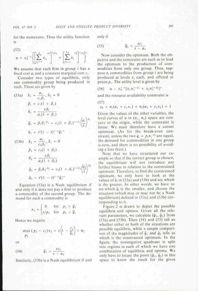
Figure 2 is drawn to depict the possibleequilibria and optima. Given all the rele-vant parameters, we calculate (q[, Q2) from(53a) and (53b). Then (54) and (55) tell uswhether either or both of the situations arepossible equilibria, while a simple compari-son of the magnitudes of ^, and 2̂ te'ls uswhich is the constrained optimum. In thefigure, the nonnegative quadrant is splitinto regions in each of which we have onecombination of equilibria and optima. Weonly have to locate the point (^i, ^2) '" thisspace to know the result for the given

306 THE AMERICAN ECONOMIC REVIEW JUNE 1977

sCjAs-a^)

FIGURE 2. SOLUTIONS LABLLED IEQUATION (53a): SOLUTIONS

REKER TO RgUATlON {53b)

TO

parameter values. Moreover, we can com-pare the location ofthe points correspond-ing to different parameter values and thusdo some comparative statics.

To understand the results, we must ex-amine how q^ depends on the relevantparameters. It is easy to see that each is anincreasing function of a, and c,- We alsofind

(58)

and we expect this to be large and negative.Further, we see from (9) that a higher {3,corresponds to a lower own-price elasticityof demand for each commodity in thatgroup. Thus ^, is an increasing function ofthis elasticity.

Consider initially a symmetric situation,with SCJ(S - fl|) ^ SC2/is - (32), fj^ = 1^2(the region G vanishes then), and supposethe point (^|, ^.) is on the boundary be-tween regions A and B. Now consider achange in one parameter, say, a higher own-elasticity for commodities in group 2. Thisraises ^2. moving the point into region A,and it becomes optimal to produce com-modities from group 1 alone. However,both (53a) and (53b) are possible Nash

equilibria, and it is therefore possible thatthe high elasticity group is produced in equi-librium when the low elasticity one shouldhave been. If the difference in elasticities islarge enough, the point moves into regionC, where (53b) is no longer a Nash equilib-rium. But, owing to the existence of a fixedcost, a significant difference in elasticities isnecessary before entry from group I com-modities threatens to destroy the "wrong"equilibrium. Similar remarks apply to re-gions Sand D.

Next, begin with symmetry once again,and consider a higher r, or a^. This in-creases^, and moves the point into regionB, making it optimal to produce the low-cost group alone while leaving both (53a)and (53b) as possible equilibria, until thedifference in costs is large enough to takethe point to region D. The change alsomoves the boundary between A and C up-ward, opening up a larger region G, butthat is not of significance here.

If both 1̂ and 2̂ are large, each group isthreatened by profitable entry from theother, and no Nash equilibrium exists, as inregions £ and F. However, the criterion ofconstrained optimality remains as before.Thus we have a case where it may be neces-sary to prohibit entry in order to sustain theconstrained optimum.

If we combine a case where c, > C2 (ora, > Qj) and &\ > ^2. ie-, where commodi-ties in group 2 are more elastic and havelower costs, we face a still worse possibility.For the point (^1, cfi) ma> then lie in regionG, where only (53b) is a possible equilib-rium and only (53a) is constrained opti-mum, i.e., the market can produce only alow cost, high demand elasticity group ofcommodities when a high cost, low demandelasticity group should have been produced.

Very roughly, the point is that althoughcommodities in inelastic demand have thepotential for earning revenues in excess ofvariable costs, they also have significantconsumers' surpluses associated with them.Thus it is not immediately obvious whetherthe market will be biased in favor of themor against them us compared with an opti-mum. Here we find the latter, and inde-pendent findings of Michael Spence in other

VOL. 67 NO. 3 DIXIT AND STIGLITZ: PRODUCT DIVERSITY 307

contexts confirm this. Similar remarksapply lo differences in marginal costs.

in the interpretation of the model withheterogenous consumers and social indil-ference curves, inelastically demanded com-modities will be the ones which are inten-sively desired by a few consumers. Thus wehave an "economic" reason why the marketwill lead to a bias against opera relative tofootball matches, and a justification forsubsidization of the former and a tax on thelatter, provided the distribution of incomeis optimum.

Even when cross elasticities are zero,there may be an incorrect choice of com-modities to be produced (relative either toan unconstrained or constrained optimum)as Figure 3 illustrates. Figure 3 illustratesa case where commodity A has a moreelastic demand curve than commodity fi; Ais produced in monopolistically competitiveequilibrium, while B is not. But clearly, itis socially desirable to produce B, since ig-noring consumer's surplus it is just mar-ginal. Thus, the commodities that arc nolproduced but ought to be are those with in-elastic demands. Indeed, if. as in the usualanalysis of monopolistic competition, elimi-nating one firm shifts the demand curve forthe other firms to the right (i.e., increasesthe demand for other firms), if the con-

output

FiGURt 4

output

FiGLRf- 3

sumer surplus from A (at its equilibriumlevel of output) is less than that from B(i.e.. the cross hatched area exceeds thestriped area), then constrained Pareto opti-mality entails restricting the production ofthe commodity with the more elasticdemand.

A similar analysis applies to commoditieswiih the same demand curves but differentcost structures. Commodity A is assumed tohave the lower fixed cost but the highermarginal cost. Thus, the average cost curvescross but once, as in Figure 4. CommodityA is produced in monopolistically com-petitive equilibrium, commodity B is not(although il is just at the margin of beingproduced). But again, observe that B shouldbe produced, since there is a large con-sumer's surplus; indeed, since were it lo beproduced. B would produce at a muchhigher level than A, there is a much largerconsumer's surplus. Thus if the governmentwere to forbid the production of /I, Bwould be viable, and social welfare wouldincrease.

In the comparison between constrainedPareto optimality and the monopolisticallycompetitive equilibrium, we have observedthat in the former, we replace some lowfixed cost-high marginal cost commoditieswith high fixed cost-low marginal cost com-modities, and we replace some commodities

308 THE AMERICAN ECONOMIC REVIEW JUNE 1977

with elastic demands with commodities withinelastic demands.

IV. Concluding Remarks

We have constructed in this paper somemodels to study various aspects of the rela-tionship between market and optimal re-source allocation in the presence of somenonconvexities, The following general con-clusions seem worth pointing out.

The monopoly power, which is a neces-sary ingredient of markets with noncon-vexities, is usually considered to distortresources away from the sector concerned.However, in our analysis monopoly powerenables firms to pay fixed costs, and entrycannot be prevented, so the relationship be-tween monopoly power and the direction ofmarket distortion is no longer obvious.

In the central case of a constant elasticityutility function, the market solution wasconstrained Parelo optimal, regardless ofthe value of that elasticity (and thus theimplied elasticity of the demand functions).With variable elasticities, the bias could goeither way, and the direction of the bias de-pended not on how the elasticity of demandchanged, but on how the elasticity of utilitychanged. We suggested that there was somepresumption that the market solutionwould be characterized by loo few firms inthe monopolistically competitive sector.

With asymmetric demand and cost condi-tions we also observed a bias against com-modities with inelastic demands and highcosts.

The general principle behind these resultsis that a market solution considers profit atthe appropriate margin, while a social opti-mum lakes into account the consumer's sur-plus. However, applications of this principlecome lo depend on details of cost and de-mand functions. We hope that the cases

presented here, in conjunction with otherstudies cited, offer some useful and newinsights.

REFERENCES

R. L. Bishop, "Monopolistic Competitionand Welfare Economics," in RobertKuenne. ed., Monopolistic CompelliionTheory. New York 1967.

E. Chamberlin, "Product Heterogeneity andPublic Policy." Amer. Econ. Rev. Proc.May 1950. "̂ 0, 85-92.

P. A. Diamond and D. L. McFadden, "SomeUses of the Expenditure Function InPublic Finance," J. Publ. Econ., Feb.1974. ,^2. 1-23.

A. K. Dixit and J. E. Stiglitz. "MonopolisticCompetition and Optimum Product Di-versity."" econ. res. pap. no. 64. Univ.Warwick. England 1975.

H. A. John Green. Aggregation in EconomicAnalysis. Princeton 1964.

H. Hotelling. "Stability in Competition."Econ.J,.UdX. 1929, J9. 41-57.

N. Kaldor,*'Market Imperfeetion and ExcessCapacity." Economica. Feb. 1934, 2,33-50.

K. Lancaster, "Socially Optimal Product Dif-ferentiation," Amer. Econ. Rev.. Sept.1975,65,567 85.

A. M. Spence, "Product Selection, FixedCosis. and Monopolistic Competition,"Rev. Econ. Stud.. June \976,43. 217-35.

D. A. Siarrett. "Principles of Optimal Loca-tion in a Large Homogeneous Area."J. Econ. Theory. Dec. 1974, 9. 418-48.

N. H. Stern, "The Optimal Size of MarketAreas." J. Econ. Theory. Apr. 1972, 4.159-73.

J. E. Sttglirz, "Monopolistic Competition inthe Capital Market." tech. rep. no. 161,IMSS, Stanford Univ.. Feb. 1975.