Molecules of Structure - Mindseye Computing, LLC · Molecules of Structure - Mindseye Computing,...
128
Molecules of Structure Page 1 of 128 Copyright © 1996,1997,2004, 2005 Jim Hines Molecules of Structure Building Blocks for System Dynamics Models Version 2.02 Jim Hines 401-301-4141 [email protected] Copyright © 1996,1997,2004, 2005 Jim Hines
Transcript of Molecules of Structure - Mindseye Computing, LLC · Molecules of Structure - Mindseye Computing,...

Molecules of Structure Page 1 of 128
Copyright © 1996,1997,2004, 2005 Jim Hines
Molecules of Structure Building Blocks for System Dynamics Models
Version 2.02
Jim Hines 401-301-4141
Copyright © 1996,1997,2004, 2005 Jim Hines

Molecules of Structure Page 2 of 128
Copyright © 1996,1997,2004, 2005 Jim Hines
Acknowledgements The molecules presented here were invented by many people – and no doubt many were invented several times independently. Tracing the ancestry of each molecule would be a large task in itself and is one that I haven’t undertaken. It would be odd though not to mention at least some of the people who are most responsible for the molecules presented here. To some extent what follows is a personal list – molecules tend to get repeated in models without attribution, so some of what I believe to be seminal work no doubt is based on yet earlier work. Still, there’s no question that many of the molecules first appeared in Jay Forrester’s writings beginning with the first published paper and the first published book in system dynamics (Forrester, J. W. (1958). Industrial Dynamics: A Major Breakthrough for Decision Makers. Harvard Business Review, 26(4), 37-66. and Forrester, J.W. (1961). Industrial Dynamics. Cambridge, MA: MIT Press). Also important was the market growth model created by Dave Packer working with Jay Forrester (Forrester, J. W. (1968). Market Growth as Influenced by Capital Investment. Industrial Management Rev. (MIT), 9(2), 83-105.). The project model, originally developed by Henry Weil, Ken Cooper, and David Peterson around 1972 contributes a number of important molecules. Jim Lyneis’ book contains important structures for corporate models (Lyneis, J. M. (1980). Corporate Planning and Policy Design. Cambridge, MA: MIT Press). Very important for me was the treasure-trove of good structures in the MIT National Model, a to which many people contributed including Alan Graham, Peter Senge, John Sterman, Nat Mass, Nathan Forrester, Bob Eberlein, and of course Jay Forrester. Many people have contributed to identifying and collecting the molecules presented here. George Richardson and Jack Pugh described a number of commonly occurring rate equations in their excellent book Introduction to System Dynamics with Dynamo (1981, MIT Press). Barry Richmond described a number of common rate structures in his 1985 paper describing STELLA, the first graphical system dynamics modeling environment (“STELLA: Software for Bringing System Dynamics to the Other 98“ in Proceedings of the 1985 International Conference of the System Dynamics Conference, Keystone Colorado, 1985, pp 706-718). Barry Richmond and Steve Peterson continued to present useful small structures in documentation for STELLA and its sister product ithink. Barry used the term “Atoms of Structure in 1985”. Misremembering that paper, I used the term “Molecules” in my own initial attempts to extend and categorize these structures in 1995. This current version of the molecules represents an expansion of the molecules covered and, most importantly, a new taxonomy for showing the connections between molecules. A taxonomy, much like a system dynamics model, is geared toward on a purpose. The purpose of the taxonomy presented here is to help people see the structural connections between models. I believe that understanding these connections make them easier to learn and makes it easier for people to create new molecules. I learned an incredible amount about taxonomy from George Hermann of MIT’s Center for Coordination Science in the
Molecules of Structure Page 3 of 128
Copyright © 1996,1997,2004, 2005 Jim Hines
process of creating a rather different taxonomy geared toward a different purpose. Before meeting George I didn’t realize that the term “world-class” could be applied to a taxonomist. But, the term fits George Hermann exactly. Bob Eberlein created a very flexible way of incorporating molecules into Vensim for the 1996 version of the collection. Bob also put the molecules up on the Vensim website which has allowed many, many people to benefit from this common heritage of our field. Gokhan Dogan spotted many, many typos in this document and then insisted that I correct them all. Of course, I secretly went back over the document to introduce a slew of new typos for you to find.

Molecules of Structure Page 4 of 128
Copyright © 1996,1997,2004, 2005 Jim Hines
Bathtub
Smooth (firstorder)
Decay
MaterialDelay
AgingChain
AgingChain
WithPDY
HinesCoflow
Traditional CascadedCoflow
Extrapolation
PresentValue
High-VisibilityPipelineCorrection
Sea AnchorPricing
MultivariateAnchoring and
Adjustment
BacklogShipping
ProtectedByLevel
SplitFlow
WorkAccom-plishmentStructure
DesiredWorkers
FromWorkFlow
EstimatedCompletion
Date
Overtime
EffectOfFatigue
Ceiling
LevelProtectedByFlow
Floor
T CoflowExperience
H CoflowExperience
Workforce
Scheduledcompletion
date
Productivity
Trend.
MarketShare
LevelProtectedByLevel
HinesCascadedCoflow
CascadedLevels
Conversion
Diffusion
firstOrderStock
Adjustment
WeightedAverage
TradCoflow
DmnlInputto f()
CloseGap
SeaAnchor andAdjustment
SmoothPricing
Producing
ProtectedSea AnchorandAdjustment
BacklogShipping
ProtectedByFlow
Low-VisibilityPipelineCorrection
ResidenceTime
ProtectedSea Anchor
Pricing
GoToZero
BrokenCascade
Smooth(higherorder)
CapacityUtilization
UnivariateAnchoring and
AdjustmentQuality
LevelProtectedByPDY
EstimatedRemainingDuration
ReducingBacklogByDoing
Work ActionFrom
Resource
FinancialFlowFromResourceWorkforce
FromBudget
Propor-tionalSplit
WeightedSplit
NonLinearSplit
Multi-dimensional
Split
ResourcesFromAction
AbilityFromAction
EstimatedProductivity
BuildingInventoryByDoingWorkDoingWork
Cascade
PopulationGrowth
CascadeProtectedByPDY
Molecules of Structure Page 5 of 128
Copyright © 1996,1997,2004, 2005 Jim Hines
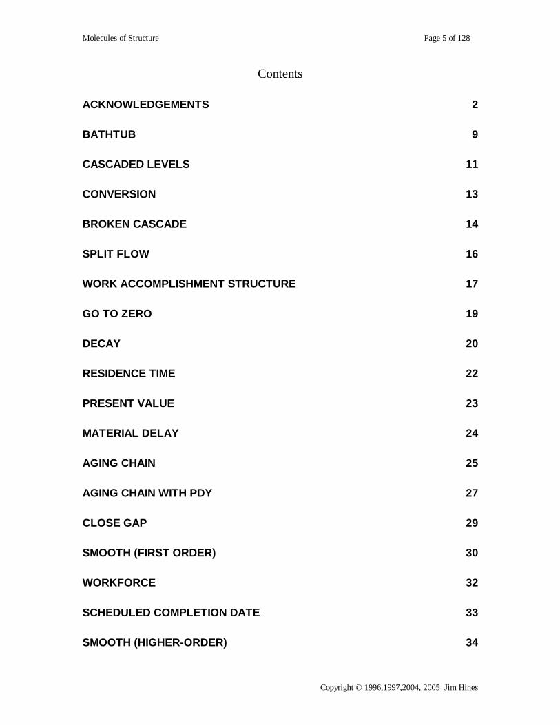
Contents
ACKNOWLEDGEMENTS 2
BATHTUB 9
CASCADED LEVELS 11
CONVERSION 13
BROKEN CASCADE 14
SPLIT FLOW 16
WORK ACCOMPLISHMENT STRUCTURE 17
GO TO ZERO 19
DECAY 20
RESIDENCE TIME 22
PRESENT VALUE 23
MATERIAL DELAY 24
AGING CHAIN 25
AGING CHAIN WITH PDY 27
CLOSE GAP 29
SMOOTH (FIRST ORDER) 30
WORKFORCE 32
SCHEDULED COMPLETION DATE 33
SMOOTH (HIGHER-ORDER) 34

Molecules of Structure Page 6 of 128
Copyright © 1996,1997,2004, 2005 Jim Hines
FIRST-ORDER STOCK ADJUSTMENT 37
HIGH-VISIBILITY PIPELINE CORRECTION 39
LOW-VISIBILITY PIPELINE CORRECTION 42
TREND 45
EXTRAPOLATION 46
COFLOW 48
COFLOW WITH EXPERIENCE 50
CASCADED COFLOW 52
DIMENSIONLESS INPUT TO FUNCTION 56
UNIVARIATE ANCHORING AND ADJUSTMENT 57
LEVEL PROTECTED BY LEVEL 59
MULTIVARIATE ANCHORING AND ADJUSTMENT 61
PRODUCTIVITY (PDY) 64
QUALITY 66
SEA ANCHOR AND ADJUSTMENT 68
PROTECTED SEA ANCHORING AND ADJUSTMENT 70
SEA ANCHOR PRICING 73
PROTECTED SEA ANCHOR PRICING 76
SMOOTH PRICING 78
EFFECT OF FATIGUE 80
Molecules of Structure Page 7 of 128
Copyright © 1996,1997,2004, 2005 Jim Hines
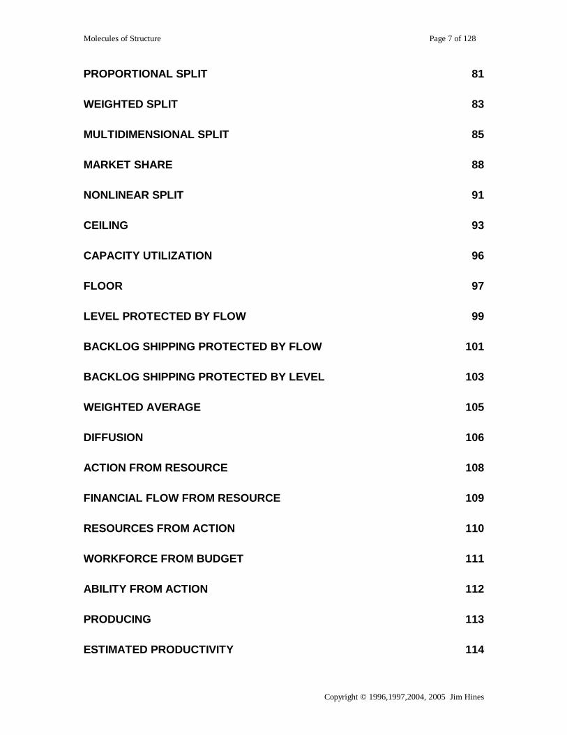
PROPORTIONAL SPLIT 81
WEIGHTED SPLIT 83
MULTIDIMENSIONAL SPLIT 85
MARKET SHARE 88
NONLINEAR SPLIT 91
CEILING 93
CAPACITY UTILIZATION 96
FLOOR 97
LEVEL PROTECTED BY FLOW 99
BACKLOG SHIPPING PROTECTED BY FLOW 101
BACKLOG SHIPPING PROTECTED BY LEVEL 103
WEIGHTED AVERAGE 105
DIFFUSION 106
ACTION FROM RESOURCE 108
FINANCIAL FLOW FROM RESOURCE 109
RESOURCES FROM ACTION 110
WORKFORCE FROM BUDGET 111
ABILITY FROM ACTION 112
PRODUCING 113
ESTIMATED PRODUCTIVITY 114

Molecules of Structure Page 8 of 128
Copyright © 1996,1997,2004, 2005 Jim Hines
DESIRED WORKFORCE FROM WORKFLOW 115
REDUCING BACKLOG BY DOING WORK 116
LEVEL PROTECTED BY PDY 117
ESTIMATED REMAINING DURATION 119
ESTIMATED COMPLETION DATE 120
OVERTIME 121
BUILDING INVENTORY BY DOING WORK 122
POPULATION GROWTH 123
DOING WORK CASCADE 124
CASCADE PROTECTED BY PDY 126

Molecules of Structure Page 9 of 128
Copyright © 1996,1997,2004, 2005 Jim Hines
LevelIncreasing Decreasing
Bathtub Immediate Parents: None
Ultimate Parents: None
Used by: Cascaded levels
Problems solved: How to increase and decrease something incrementally.
Equations:
Level = INTEG(Increasing-Decreasing,___) Units: widgets Decreasing = ___ Units: widgets/year Increasing = ___ Units: widgets/year Description: A bathtub accumulates the difference between its inflow and its outflow. A physical example is an actual bathtub. The level of water is increased by the inflow from the tap and decreased by the outflow at the drain.
Classic examples: A workforce might be represented as a bathtub whose inflow is hiring and whose outflows is attrition. A final-goods inventory could be a bathtub whose inflow is arrivals of product and whose outflow is unit sales. Factories could be represented as a bathtub whose inflow is construction and whose outflow is physical depreciation. Retained earnings could be represented as a bathtub with revenues as the inflow and outflow of expenses.
Caveats: Often bathtubs represent physical accumulations which should not take on negative values. To prevent negative values, the outflow must be influenced directly by the level. This is termed “first order feedback” (i.e. a feedback loop is created that includes only one level (a feedback loop with two levels would be “second order”). Molecules employing first-order feedback include smooths, decays, and protected levels (e.g. level protected by level and level protected by flow).
Technical notes: A bathtub is simply an integration of one inflow and one outflow. System dynamics takes an integral view of calculus, which is reflected in the form that level equations take in all system dynamics languages (DYNAMO, Vensim, iThink, Powersim, etc.)
∫ −+=T
TttTT dtoutflowinflowLevelLevel
00
)(
or, in modified DYNAMO notation

Molecules of Structure Page 10 of 128
Copyright © 1996,1997,2004, 2005 Jim Hines
)(* dttdttdttt outflowinflowdtLevelLevel −−− −+=
The idea is expressed in the differential calculus as
ttt outflowinflow
dtLeveld −=

Molecules of Structure Page 11 of 128
Copyright © 1996,1997,2004, 2005 Jim Hines
Cascaded levels (also known as “chain”)
Level 1 Level 2 Level 3flowingIn movingTo
Level2movingTo
Level3flowingOut
Immediate Parents: Bathtub Ultimate Patents: Bathtub
Used by: Conversion, Aging chain, Broken cascade, Smooth (higher order), Traditional cascaded coflw, Doing work cascade
Problem solved: How to represent something that accumulates at a number of points instead of just one.
Equations: flowingIn = ____ Units: material/Month flowingOut = ____ Units: material/Month Level 1 = INTEG(flowingIn-movingToLevel2, ____) Units: material Level 2 = INTEG(movingToLevel2-movingToLevel3, ____) Units: material Level 3 = INTEG(movingToLevel3-flowingOut, ____) Units: material movingToLevel2 = ____ Units: material/Month movingToLevel3 = ____ Units: material/Month Description: A cascade is a set of levels, where one level’s outflow is the inflow to a second level, and the second level’s outflow is the inflow to a third, etc. A cascade can be seen as a structure that divides up an accumulation into “sub-accumulations”. The number of levels in a cascade can be any number greater than two.
Behavior: Because the rates are not defined, behavior is not defined.
Classic examples: Items being manufactured accumulate at many points in the system, perhaps in front of each machine in a production line as well as in finished inventory. Conceptually it is possible to have a chain with a level for each machine. Usually this is too detailed for a system dynamics model; instead we represent material accumulating in a smaller number of levels, perhaps three: manufacturing starts, work in process, and finished inventory.

Molecules of Structure Page 12 of 128
Copyright © 1996,1997,2004, 2005 Jim Hines
A measles epidemic model might represent people in three stages (levels): susceptible, infected, and recovered. (See Aging Chain molecule)
A workforce might be composed of three stocks: Rookies, Experienced, and Pros. As they are hired, people flow into the rookies level from which they flow in the level of experienced employees. Experienced employees flow into the stock of pros, which is depleted by people retiring. (See Aging Chain molecule).
Caveats: Often the levels represent physical accumulations which should not go negative. See caveats under Level.
Technical notes: In nature, there are phenomena which combine the characteristics of both flows and stocks. A river, for example, is both a rate of flow and has volume. In system dynamics modeling we represent the world as consisting of pure flows having no volume; and pure levels having no flow. We view a river as being composed of a chain of “lakes”, each having a volume, connected by flows each being a pure rate: The water accumulates only in the “lakes” not in the flows. A river might be represented as a cascade of two levels: an upstream stock and a downstream stock. This “lumped parameter” view of the world permits the use of integral equations. To represent flows that have volume would require the more complicated mathematics of partial integral (partial differential) equations. Such a view of the world is more difficult to model and more time consuming to simulate.

Molecules of Structure Page 13 of 128
Copyright © 1996,1997,2004, 2005 Jim Hines
Conversion Immediate parents: Cascaded levels Ultimate parents: Bathtub
Used by: Diffusion
Problem solved: How to represent people changing their status. E.g. from non-believer to believer, from non-customer to customer, from non-infected to infected
Equations:
Source of converts = INTEG(-converting, ___) Units: people converting = ___ Units: people/Year Converts = INTEG(cnverting, ___) Units: people Description: People flow from one category to the other
Behavior: Converting is undefined, so behavior is undefined
Classic examples: Used in diffusion models
Caveats: None
Technical notes: None
ConvertsSource ofconverts converting
Molecules of Structure Page 14 of 128
Copyright © 1996,1997,2004, 2005 Jim Hines
Broken Cascade
ordersInProcess
inventory
ordering ordersBeingFulfilled
shippingreceivingInventory
avgOrderSize
Level 1
Level 2
inflowToLevel1
outflowFromLevel1
outflowFromLevel2
inflowToLevel2
General Form
Example
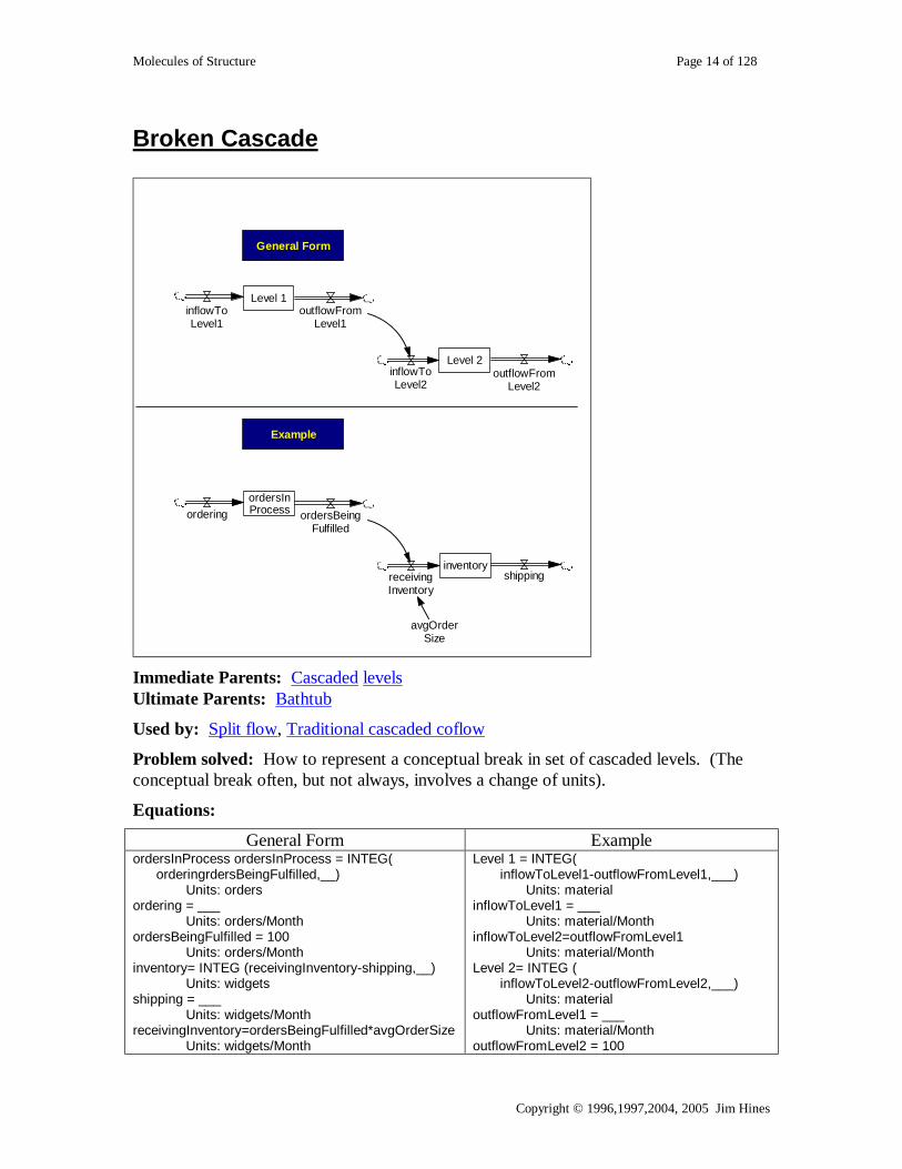
Immediate Parents: Cascaded levels Ultimate Parents: Bathtub
Used by: Split flow, Traditional cascaded coflow
Problem solved: How to represent a conceptual break in set of cascaded levels. (The conceptual break often, but not always, involves a change of units).
Equations:
General Form Example ordersInProcess ordersInProcess = INTEG( orderingrdersBeingFulfilled,__)
Units: orders ordering = ___
Units: orders/Month ordersBeingFulfilled = 100
Units: orders/Month inventory= INTEG (receivingInventory-shipping,__)
Units: widgets shipping = ___
Units: widgets/Month receivingInventory=ordersBeingFulfilled*avgOrderSize
Units: widgets/Month
Level 1 = INTEG( inflowToLevel1-outflowFromLevel1,___) Units: material inflowToLevel1 = ___ Units: material/Month inflowToLevel2=outflowFromLevel1 Units: material/Month Level 2= INTEG ( inflowToLevel2-outflowFromLevel2,___) Units: material outflowFromLevel1 = ___ Units: material/Month outflowFromLevel2 = 100

Molecules of Structure Page 15 of 128
Copyright © 1996,1997,2004, 2005 Jim Hines
avgOrderSize=_________ Units: widgets/order
Units: material/Month
Description: A broken cascade is a cascade where the outflow of one level, rather than flowing directly into the next level, instead terminates in a cloud. The inflow to the next level is then a function of the prior outflow. If the inflow to the next level is equal to the outflow from the prior level (e.g. receivengInventory = ordersBeingFulfilled), then the broken cascade is mathematically equivalent to the regular cascade. Often the inflow to the next stock is the outflow from the stock multiplied by a constant that represents a change of units (e.g. avgOrderSize in the example above.
Behavior: Behaves like a regular cascade
Classic examples: In modeling a supply chain, there is often a conceptual break from raw materials inventory to work in process. The conceptual break often also involves a change in units.
Caveats: None
Technical notes: None

Molecules of Structure Page 16 of 128
Copyright © 1996,1997,2004, 2005 Jim Hines
Split Flow Immediate Parents: Broken cascade Ultimate Parents: Bathtub Used by: Work accomplishment structure, Low-visibility pipeline correction Problem solved: How to disaggregate an outflow into sub-flows Equations: Source Stock = INTEG(-Aggregate Outflow,____) Units: Widgets2 Aggregate Outflow = ____ Units: Widgets/Month First Subflow = Aggregate Outflow*Fractional Split to First Subflow Units: Widgets/Month Fractional Split to First Subflow = ____ Units: fraction First Destination Stock = INTEG(First Subflow,0) Units: Widgets Second Subflow = Aggregate Outflow*(1-Fractional Split to First Subflow) Units: Widgets/Month Second Destination Stock = INTEG(Second Subflow, ____) Units: Widgets Description: This structure splits an outflow into two (or more) subflows into other levels (or into sinks).. Behavior: Aggregate outflow is undefined, so behavior is undefined. Classic examples: Work Accomplishment Structure Caveats: None Technical notes: Traditionally the split outflow is represented with the aggregate flow going into a sink (cloud) and the two sub-flows coming out of sources (clouds). Although not standard, it is possible to draw the pipe splitting in two. The equations remain the same.
SourceStock
SecondDestination
Stock
FirstDestination
Stock
AggregateOutflow
FirstSubflow
SecondSubflow
Fractional Split toFirst Subflow

Molecules of Structure Page 17 of 128
Copyright © 1996,1997,2004, 2005 Jim Hines
Work Accomplishment Structure Also known as Rework Cycle Immediate Parents: Split Flow Ultimate Parents: Bathtub Used by: None Problem solved: How to represent rework Equations: WorkToDo = INTEG( DiscoveringRework – AccomplishingWork,___) Units: SquareFeet DiscoveringRework = ___ Units: SquareFeet/Week AccomplishingWork = ___ Units: SquareFeet/Week CorrectWork = INTEG( AccomplishingCorrectly , 0) Units: SquareFeet AccomplishingCorrectly = AccomplishingWork * Quality Units: SquareFeet/Week Quality = ___ Units: fraction UndiscoveredRework = INTEG( AccomplishingIncorrectly - DiscoveringRework ,___) Units: SquareFeet AccomplishingIncorrectly = AccomplishingWork * ( 1 - Quality ) Units: SquareFeet/Week Description: We begin with some work to do and begin to accomplish it by some process (perhaps by the producing molecule). Some of the work is done correctly, but some is not. Quality is the fractional split. Quality here has a very narrow definition: the fraction of work that is being done correctly. The work that is not done correctly flows into undiscovered rework, where it sits until it is discovered (again by a process not shown). When it is discovered it flows into work to be (re) done. Note that the stock of undiscovered rework is not knowable by decision makers “inside” the model. The stock is really there, but no-one, except the modeler and god, know how much it holds. Behavior: Work can make many cycles.
WorkToDo
CorrectWork
UndiscoveredRework
AccomplishingWork
AccomplishingCorrectly
AccomplishingIncorrectly
DiscoveringRework
Quality

Molecules of Structure Page 18 of 128
Copyright © 1996,1997,2004, 2005 Jim Hines
Classic examples: This is the classic project structure. It was originally developed by Pugh-Roberts, which continues to use and develop the structure. The structure is at the heart of Terek Abdel-Hamid’s work on software project management. Today it is used by a number of consultants and consulting firms. Caveats: none Technical notes: The structure, as shown does not contain the definition of accomplishing work or discovering rework. Typically these flows are formulated using the producing molecule, although discovering rework is sometimes represented as a Go to Zero (i.e. undiscovered rework is represented as a material delay). Quality is usually formulated as an anchoring and adjustment molecule. Often the discovered rework flows into a level that keeps it separate from the original work to do -- this permits one to model a productivity and a quality on rework that are potentially different from productivity and quality on original work.

Molecules of Structure Page 19 of 128
Copyright © 1996,1997,2004, 2005 Jim Hines
Go To Zero Immediate Parents: None Ultimate Parents: None
Used by: Decay, Backlog shipping protected by flow, Level protected by flow
Problem solved: How to generate an action (i.e. a flow) that will move a current value (of a stock) to zero over time.
Equations:
ActionToGo to zero = CurrentValue/timeToGo to zero Units: widgets/Month CurrentValue = ___ Units: widgets timeToGo to zero = ___ Units: months Description: The action (or rate of flow) that will take a quantity (a stock) to zero over a given time is simply the quantity divided by the given time.
Behavior: No stocks, so no behavior
Classic examples: The outflow of a decay or material delay. The desired shipping in a Backlog shipping protected by flow molecule.
Caveats: When time “constant” (timeToGo to zero) is formulated as a variable, care should be taken to ensure its value can not become zero to avoid a divide-by-zero error.
Technical notes: The intuition behind this formulation is the following: Consider a variable whose current value is CurrentValue. The variable will become zero in exactly timeToGo to zero months if the variable declines at a constant rate equal to actionToGo to zero. Usually, however, the actionToGo to zero will not remain constant, because the action itself will change the currentValue and/or value of timeToGo to zero. Consequently, the variable in question will typically not be zero after timeToGo to zero months. Depending on the actual formulation, the timeToGo to zero often will have a real world meaning. In the case of a decay, for example, the average time for an aggregate of things (e.g. a group of depreciating machines) to decline to zero is equal to timeToGo to zero.
Other molecules that can generate an action (or a flow) include close gap (and its children) and flow from resource (and its children)
CurrentValue
timeToGoToZero
ActionToGoToZero
Molecules of Structure Page 20 of 128
Copyright © 1996,1997,2004, 2005 Jim Hines
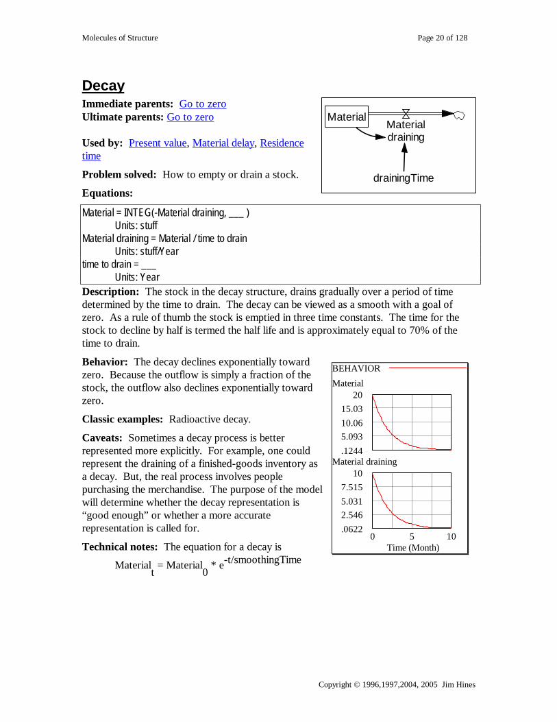
Decay Immediate parents: Go to zero Ultimate parents: Go to zero Used by: Present value, Material delay, Residence time
Problem solved: How to empty or drain a stock.
Equations:
Material = INTEG(-Material draining, ___ ) Units: stuff Material draining = Material / time to drain Units: stuff/Year time to drain = ___ Units: Year Description: The stock in the decay structure, drains gradually over a period of time determined by the time to drain. The decay can be viewed as a smooth with a goal of zero. As a rule of thumb the stock is emptied in three time constants. The time for the stock to decline by half is termed the half life and is approximately equal to 70% of the time to drain.
Behavior: The decay declines exponentially toward zero. Because the outflow is simply a fraction of the stock, the outflow also declines exponentially toward zero.
Classic examples: Radioactive decay.
Caveats: Sometimes a decay process is better represented more explicitly. For example, one could represent the draining of a finished-goods inventory as a decay. But, the real process involves people purchasing the merchandise. The purpose of the model will determine whether the decay representation is “good enough” or whether a more accurate representation is called for.
Technical notes: The equation for a decay is
Materialt = Material
0 * e-t/smoothingTime
BEHAVIORMaterial
2015.0310.065.093.1244
Material draining10
7.5155.0312.546.0622
0 5 10Time (Month)
MaterialMaterialdraining
drainingTime

Molecules of Structure Page 21 of 128
Copyright © 1996,1997,2004, 2005 Jim Hines
The half life can be determined from this equation to be: ln(0.5)*timeToDrain. ln(0.5) is approximately 0.7. The outflow from the decay is distributed exponentially. The average residence time of material in the level is equal to the timeToDrain.

Molecules of Structure Page 22 of 128
Copyright © 1996,1997,2004, 2005 Jim Hines
Residence Time Immediate Parents: Decay Ultimate parents: Go to zero Used by: None
Problem solved: How to determine the average residence time of items flowing through a stock.
Equations:
AverageResidenceTime = Material/Material draining Units: Year Material = INTEG(-Material draining, ___) Units: items Material draining = ___ Units: items/Year Description: This is based on the same understanding as that behind the decay; however the inputs and outputs are switched. Here, we know the rate at which material is draining (as well as the stock) and we calculate the average time to drain (i.e. the average residence time).
Behavior: No feedback, so no endogenous dynamic behavior
Classic examples: None
Caveats: None
Technical notes: This is based on Little’s Law. In equilibrium the calculation for the average residence time is correct, no matter what process is actually draining the level. To derive the formula for the specific process of a decay provides the intuition. The equation for a decay’s outflow is.
t
tt decayTime
StockowdecayOutfl =
The above equation says that if we know the values of the Stock and the value of the decayTime, we can figure out the value of the decayOutflow. Now if we already know the value of the decayOutflow (as well as the Stock’s value) but we don’t know the decayTime’s value, we can re-arrange the above equation to yield
t
tt owdecayOutfl
StockdecayTime = .
Which is an equation that allows us to figure out the decayTime if we know the other two quantities. The equation above is the Residence Time molecule.
MaterialMaterialdraining
AverageResidenceTime

Molecules of Structure Page 23 of 128
Copyright © 1996,1997,2004, 2005 Jim Hines
Present value Immediate parents: Decay Ultimate parents: Go to zero Used by: None
Problem solved: How to calculate the present value of a cash stream.
Equations:
PresentValueOfProfits = INTEG(IncreasingPresentValue, ___) Units: $ IncreasingPresentValue = Profits * DiscountingFactor Units: $/Year Profits = Units: $/Year DiscountingFactor = INTEG( - ReducingDiscountingFactor, 1) Units: fraction DiscountRate = ___ Units: fraction / Year ReducingDiscountingFactor = DiscountRate * DiscountingFactor Units: fraction / Year Description: The present value of a cash stream (e.g. profits) is simply the accumulation of profits, weighted at each instant by a discounting factor. The discounting factor decays at a rate determined by the discounting factor.
Classic examples: Discounted profits.
Caveats: None.
Technical notes: A discount rate of 0.10 (10%) is equivalent to a time constant of 10 years on the decay structure that represents the discounting factor. (See note on decay molecule).
PresentValueOfProfits
Profits
DiscountFactor
DiscountRate
IncreasingPresentValue
ReducingDiscounting
Factor

Molecules of Structure Page 24 of 128
Copyright © 1996,1997,2004, 2005 Jim Hines
Material Delay Immediate parents: Decay Ultimate parents: Go to zero Used by: Aging chain
Problem solved: How to delay a flow of material.
Equations:
Material flowing out = Material / Time to flow out Units: stuff/Year Time to flow out = ___ Units: Year Material = INTEG(Material flowing in-Material flowing out, Material flowing in*Time to flow out) Units: stuff Material flowing in = ___ Units: stuff/Year Description: The material delay creates a delayed version of a flow by accumulating the flow into a level and then draining the level over some time constant (timeToFlowOut). The outflow from the level is a delayed version of the inflow. The average time by which material is delayed is equal to the time constant.
Classic examples: A flow of material is shipped and received after a delay. The stock in this case is the material in transit.
Caveats: None.
Technical notes: The actual delay times for the items that comprise the flow are distributed exponentially with a mean of the time constant. Instead of dividing by a time constant, one can multiply by a fractional decay rate. For example, a 10 year time constant would correspond to a decay rate of 0.10 (10%) per year.
MaterialMaterial
flowing out
Time toflow out
Materialflowing in

Molecules of Structure Page 25 of 128
Copyright © 1996,1997,2004, 2005 Jim Hines
Aging Chain Also known as Cascaded Delay
Newmaterial Materialmaturing
Time tomature
Materialflowing in
Maturematerial
OldmaterialMaterial
agingMaterial
flowing out
Time to ageTime to flow
out
Immediate parents: Material delay, Cascaded levels Ultimate parents: Bathtub, Go to zero Used by: Capacity Ordering, Aging Chain with PDY, Hines Cascaded Coflow, Traditional Cascaded Coflow
Problem solved: How to drain a stock so that the outflow is hump shaped, that is more “normally” distributed. How to create a chain of stocks.
Equations:
New material = INTEG(Material flowing in-Material maturing,Material flowing in*Time to mature) Units: stuff Material flowing in = ___ Units: stuff/Year Material maturing = New material / Time to mature Units: stuff/Year Time to mature = Units: Year Mature material = INTEG(Material maturing-Material aging, Material maturing*Time to age) Units: stuff Material aging = Mature material/Time to age Units: stuff/Year Time to age = ___ Units: Year Old material = INTEG(Material aging-Material flowing out, Material aging*Time to flow out) Units: stuff Material flowing out = Old material/Time to flow out Units: stuff/Year Time to flow out = ___ Units: years Description: An aging chain is a cascade of material delays. Although, the example above has three stocks (a third-order aging chain), an aging chain can have any number of
Molecules of Structure Page 26 of 128
Copyright © 1996,1997,2004, 2005 Jim Hines
stocks greater than two. Sometimes only the average time it takes an item to transit the entire chain is known and the time constants associated with each individual flow are not known. In this case, simply set each time constant equal to the overall transit time divided by the number of stocks in the chain. That is the delay for stock i is defined as
nocksInChainumberOfSttotalDelaydelayi =
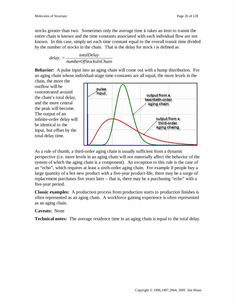
Behavior: A pulse input into an aging chain will come out with a hump distribution. For an aging chain whose individual-stage time constants are all equal, the more levels in the chain, the more the outflow will be concentrated around the chain’s total delay, and the more central the peak will become. The output of an infinite-order delay will be identical to the input, but offset by the total delay time.
As a rule of thumb, a third-order aging chain is usually sufficient from a dynamic perspective (i.e. more levels in an aging chain will not materially affect the behavior of the system of which the aging chain is a component). An exception to this rule is the case of an “echo”, which requires at least a sixth-order aging chain. For example if people buy a large quantity of a hot new product with a five-year product-life, there may be a surge of replacement purchases five years later – that is, there may be a purchasing “echo” with a five-year period.
Classic examples: A production process from production starts to production finishes is often represented as an aging chain. A workforce gaining experience is often represented as an aging chain.
Caveats: None
Technical notes: The average residence time in an aging chain is equal to the total delay.

Molecules of Structure Page 27 of 128
Copyright © 1996,1997,2004, 2005 Jim Hines
Aging Chain with PDY Parents: Aging chain
Used by: None
Problem solved: How to represent a workforce where people gain experience they become more productive.
Equations:
Production = ExperiencedProduction+GrayHairProduction+RookieProduction Units: widgets/Year RookieProduction = Rookies*RookieProductivity Units: widgets/Year RookieProductivity = ___ Units: widgets/person/Year Rookies = INTEG(Hiring - Maturing, Hiring*TimeForRookiesToMature ) Units: people Hiring = ___ Units: people/Year Maturing = Rookies / TimeForRookiesToMature Units: people/Year TimeForRookiesToMature = ___ Units: years ExperiencedProduction = Experienced*ExperiencedProductivity Units: widgets/Year ExperiencedProductivity= ___ Units: widgets/person/Year Experienced = INTEG(Maturing - GainingWisdom, Maturing *TimeToGainWisdom ) Units: people GainingWisdom = Experienced / TimeToGainWisdom Units: people/Year TimeToGainWisdom = ___ Units: years GrayHairProduction = GrayHairs*GrayHairProductivity Units: widgets/Year GrayHairProductivity = ___ Units: widgets/person/Year
Rookies Experienced GrayHairsHiring Maturing Gaining
WisdomRetiring
TimeForRookiesTo
Mature
TimeToGainWisdom
TimeForGrayHairToRetire
production
RookieProductivity
GrayHairProductivity
ExperiencedProductivity
RookieProduction
ExperiencedProduction
GrayHairProduction

Molecules of Structure Page 28 of 128
Copyright © 1996,1997,2004, 2005 Jim Hines
GrayHairs = INTEG(GainingWisdom - Retiring, GainingWisdom*TimeForGrayHairToRetire ) Units: people Retiring = GrayHairs / TimeForGrayHairToRetire Units: people/Year TimeForGrayHairToRetire = ___ Units: Year
Description: This is an aging chain of people, where each level also has an (optional) added decay structure to represent attrition. Each category of people has a different productivity. Total production is simply the sum of each category working at its own productivity.
Behavior: See notes for decay and for Cascaded delay or aging chain
Classic examples: A common structure for representing difficulties encountered when a company must grow -- and, hence, expand employment - quickly.
Caveats: Gaining of experience is purely a function of time, rather than a function of doing the work. The latter would be more accurate in most situations, but the structure as formulated is simpler and often good enough. The rule of thumb for DT (see Caveats under Smooth) must be amended because each level has two outflows -- DT should be one fourth to one tenth of the effective time constant which may be quite short (see technical note).
Technical notes: The outflow from any one level is
Outflow = Level/τ + Level * η where τ is the time it takes on average to move to the next category and η is the fractional attrition rate for people in the category Or, Outflow = Level / (τ/(1 + ητ))
So DT needs to be shorter than 1/4 to 1/10 of the effective time constant: (τ/(1 + ητ)
Molecules of Structure Page 29 of 128
Copyright © 1996,1997,2004, 2005 Jim Hines
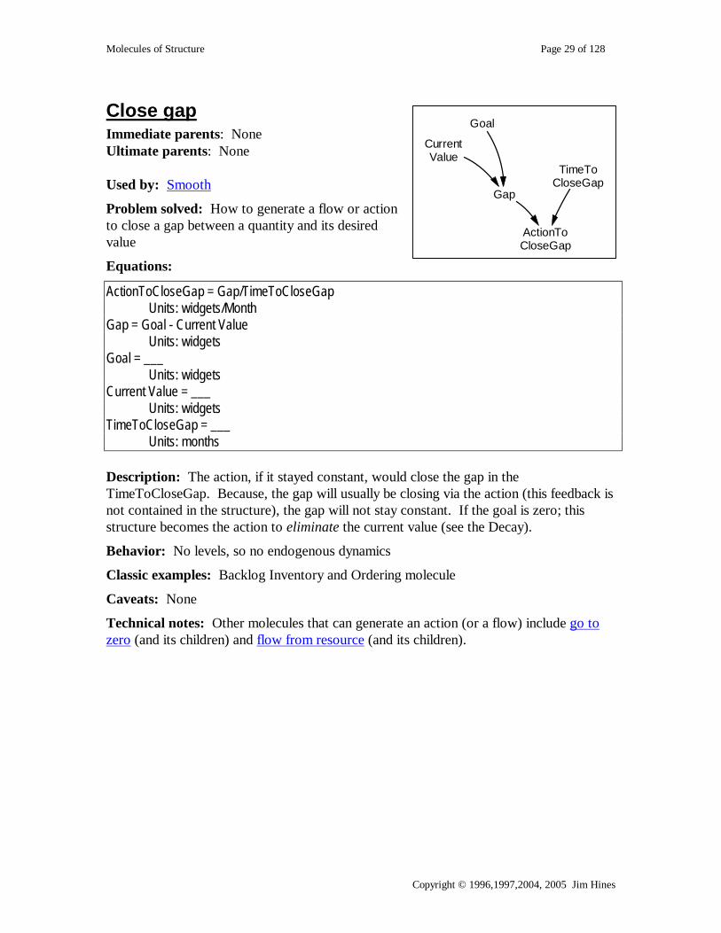
Close gap Immediate parents: None Ultimate parents: None Used by: Smooth
Problem solved: How to generate a flow or action to close a gap between a quantity and its desired value
Equations:
ActionToCloseGap = Gap/TimeToCloseGap Units: widgets/Month Gap = Goal - Current Value Units: widgets Goal = ___ Units: widgets Current Value = ___ Units: widgets TimeToCloseGap = ___ Units: months Description: The action, if it stayed constant, would close the gap in the TimeToCloseGap. Because, the gap will usually be closing via the action (this feedback is not contained in the structure), the gap will not stay constant. If the goal is zero; this structure becomes the action to eliminate the current value (see the Decay).
Behavior: No levels, so no endogenous dynamics
Classic examples: Backlog Inventory and Ordering molecule
Caveats: None
Technical notes: Other molecules that can generate an action (or a flow) include go to zero (and its children) and flow from resource (and its children).
CurrentValue
Goal
Gap
ActionToCloseGap
TimeToCloseGap

Molecules of Structure Page 30 of 128
Copyright © 1996,1997,2004, 2005 Jim Hines
Smooth (first order) Immediate parents: Close gap Ultimate parents: Close gap
Used by: First-order stock adjustment, Hines coflow, Traditional coflow, Trend, Effect of fatigue, Workforce, Scheduled completion date, Sea Anchor and Adjustment
Problem solved: How to have a quantity gradually and smoothly move toward a goal. How to delay information. How to represent a perceived quantity. How to smooth information. How to represent an expectation.
Equations:
smoothed quantity = INTEG(updating smoothed quantity, quantity) Units: stuff updating smoothed quantity = Gap / smoothing time Units: stuff/Year smoothing time = ___ Units: Year Gap = quantity - smoothed quantity Units: stuff quantity = ___ Units: stuff
Description: A smooth is a level with a specific inflow/outflow formulation. The inflow is formulated as a net rate (i.e. negative values of the “inflow” decrease the level). The rate of change is intended to “close the gap”. The gap is the difference between some goal and the smooth itself.
Behavior: The stock adjusts toward the goal exponentially. As illustrated at the right for a step increase in the goal.
The gap between the stock and the goal is closed according to the constant (the smoothing time). Intuitively, the magnitude of the gap would decline to zero over the smoothing time if the net inflow were held constant. In fact, the net inflow changes continuously as the level changes. The rule of thumb is that the gap is almost completely eliminated within
Step Increase300
250
200
150
1000 1 2 3 4 5 6 7 8 9 10
Time (Month)
smoothed quantity - BEHAVIOR stuffquantity - BEHAVIOR stuff
smoothedquantity updating smoothed
quantity
goal
Gap
smoothing time

Molecules of Structure Page 31 of 128
Copyright © 1996,1997,2004, 2005 Jim Hines
three time constants. If the goal is oscillating the smooth will also oscillate with a lag and with a reduced amplitude. The lag gives rise to the use of a smooth a delay. The reduced amplitude gives rise to using the smooth as means of “smoothing out” random ups and downs in the goal.
Classic examples: The smooth is used in virtually every system dynamics model. A classic example is a cooling cup of coffee. The temperature of the coffee can be represented as the stock; the goal is the temperature of the air surrounding around the cup. The temperature of the coffee gradually adjusts to equal the air temperature. The time constant is determined by the volume of coffee and the insulating properties of the cup. Adaptive expectations are modeled with a smooth. Say one is forming a judgment of how many projects a consultant can sell in a month. If sales have been roughly half a project per month, but in September sales jump to two; we perhaps adjust our expectations upward a bit, but not to two sales per month. If sales stay at around two per month, though we gradually will come to expect that number of sales. A smooth is the structure to capture this.
Caveats: When using Euler integration, a large DT (Time Step) can give rise to integration error which will show up as very rapid oscillations of the stock. As a rule of thumb DT should be no larger than 1/4 to 1/10 of the time constant.
Technical notes: If the goal is held constant, the smooth can be expressed mathematically as
SmoothedQuantityt =
Goal - (Goal - SmoothedQuantity0)e-t/smoothingTime
The “three time constants to close the gap” comes from the above equation. For any
number n of time constants the original gap is multiplied by a e-n. In particular in three
time constants, the gap is reduced to e-3 ≈ 5% of its original size.

Molecules of Structure Page 32 of 128
Copyright © 1996,1997,2004, 2005 Jim Hines
Workforce Immediate parents: Smooth (first order) Ultimate parents: Close gap Used by: Overtime
Problem solved: How to represent the number of people working on a project
Equations: Workforce = INTEG( Hiring and Firing , DesiredPeople ) Units: people Hiring and Firing = Worker Shortage / time to hire or fire Units: people/Year time to hire or fire = Units: Year Worker Shortage = DesiredPeople - Workforce Units: people DesiredPeople = Units: people
Description: The workforce is just a smooth of the desired workforce. This means that people will be hired or fired to (gradually) move the actual workforce to the desired level.
Behavior: Obvious
Classic examples: This is often used in models of projects
Caveats: None
Technical notes: Time to hire or fire aggregates a number of lags including: the time for someone to realize that the workforce is not at the correct level, the time to communicate this realization, the time to get authorization for a new workforce level, the time to advertise for workers, the time to interview them, the time to actually bring them on board, and the time to bring them up to speed as fully productive workers.
Note: The essence of this molecule is that the workforce is a smooth of DesiredPeople. Although DesiredPeople is often formulated as a Desired workforce molecule; there is no requirement that this be the case. Consequently, this molecule is not a child of Desired workforce.
WorkforceHiring and
Firing
DesiredPeople
WorkerShortage
time tohire or fire

Molecules of Structure Page 33 of 128
Copyright © 1996,1997,2004, 2005 Jim Hines
Scheduledcompletion
dateScheduleUpdating
Time to changeschedule
EstimatedCompletion
Date
Scheduled Completion Date
Immediate parents: Smooth (first order), Ultimate parents: Close gap
Used by: None
Problem solved: How to represent the process by which the scheduled completion date is set.
Equations:
Scheduled completion date = INTEG( ScheduleUpdating , EstimatedCompletionDate ) Units: week ScheduleUpdating = ( EstimatedCompletionDate - Scheduled completion date ) / Time to change schedule
Units: weeks/week Time to change schedule = ___ Units: week EstimatedCompletionDate = ___ Units: week Description: The scheduled completion date adjusts toward the estimated completion date. The scheduled completion date is simply a smooth of the estimated.
Behavior: Obvious
Classic examples: Used in project models
Caveats: None
Technical notes: None

Molecules of Structure Page 34 of 128
Copyright © 1996,1997,2004, 2005 Jim Hines
Smooth (higher-order) Also known as cascaded smooth.
Smooth1updatingsmooth1
goal
Gap1
smoothing time1
Smooth2updatingsmooth2
Gap2
smoothing time2
Smooth3.updatingsmooth3
Gap3
smoothing time3
Immediate Parents: Smooth (first order), Cascaded levels Ultimate Parents: Close gap, Bathtub
Used by: Hines cascaded coflow
Problem solved: How to create a “smooth” where the adjustment toward the goal starts out slowly, gains speed, and then slows for the final approach. How to model a situation where people are slow to initially perceive a change, but ultimate do catch on completely.
Equations:
Smooth1 = INTEG( updating smooth1 , goal ) Units: stuff updating smooth1 = Gap1 / smoothing time1 Units: stuff/Year smoothing time1 = ___ Units: Year Gap1 = goal - Smooth1 Units: stuff goal = ___ Units: stuff Smooth2 = INTEG( updating smooth2 , Smooth1 ) Units: stuff updating smooth2 = Gap2 / smoothing time2 Units: stuff/Year smoothing time2 = ___ Units: Year Gap2 = Smooth1 - Smooth2 Units: stuff "Smooth3." = INTEG( updating smooth3 , Smooth2 )

Molecules of Structure Page 35 of 128
Copyright © 1996,1997,2004, 2005 Jim Hines
Units: stuff updating smooth3 = Gap3 / smoothing time3 Units: stuff/Year smoothing time3 = 2 Units: Year Gap3 = Smooth2 - "Smooth3." Units: stuff Description: A higher order smooth is a cascade of two or more smooths where each smooth becomes the goal of the immediately following smooth. The stock of final smooth is often considered the “output” variable -- that is the variable that’s ultimately adjusting toward the goal. The usual case is to have the same delay at each stage of the smooth. That is if k is a constant
OagaggregateLk
kOrderkagaggregateL
iOrder
Orderiklag
Orderi
i
i
=
==
=∀=
∑=
=
as defined isk elseor
*
as defined is lag) average (or the agaggregateL either the whereand
stage individual eachfor lag theisk cascade thein stage particularany is
delay theoforder theis where
...1
1
For example in the usual case where the individual lags are all the same, if the aggregate
lag is, say, thirty weeks, then the lag for each stage will be weeks103
weeks30= .
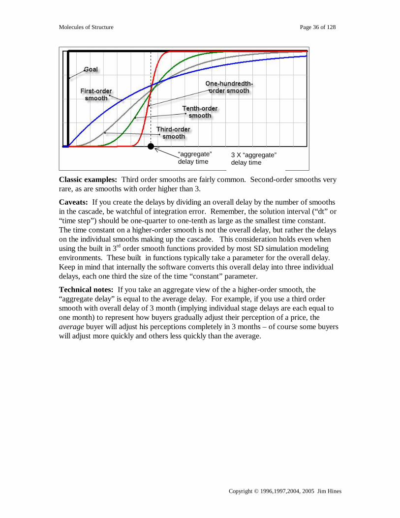
Behavior: In the case where the individual-stage lags are all the same, the adjustment will become more sudden and more concentrated at the point of the aggregate lag. All of the adjustment would happen at the aggregate lag in the case of an infinite-order smooth. (Note in such a case the aggregate lag is a finite real number and each individual-stage lag
is an infinitesimal, intuitively ∞
=Orderk which is an infinitesimal. The infinite-order
smooth’s response to a step is another step offset from the original by the overall (or aggregate) lag.
Molecules of Structure Page 36 of 128
Copyright © 1996,1997,2004, 2005 Jim Hines
Classic examples: Third order smooths are fairly common. Second-order smooths very rare, as are smooths with order higher than 3.
Caveats: If you create the delays by dividing an overall delay by the number of smooths in the cascade, be watchful of integration error. Remember, the solution interval (“dt” or “time step”) should be one-quarter to one-tenth as large as the smallest time constant. The time constant on a higher-order smooth is not the overall delay, but rather the delays on the individual smooths making up the cascade. This consideration holds even when using the built in 3rd order smooth functions provided by most SD simulation modeling environments. These built in functions typically take a parameter for the overall delay. Keep in mind that internally the software converts this overall delay into three individual delays, each one third the size of the time “constant” parameter.
Technical notes: If you take an aggregate view of the a higher-order smooth, the “aggregate delay” is equal to the average delay. For example, if you use a third order smooth with overall delay of 3 month (implying individual stage delays are each equal to one month) to represent how buyers gradually adjust their perception of a price, the average buyer will adjust his perceptions completely in 3 months – of course some buyers will adjust more quickly and others less quickly than the average.
“aggregate” delay time
3 X “aggregate” delay time
Molecules of Structure Page 37 of 128
Copyright © 1996,1997,2004, 2005 Jim Hines
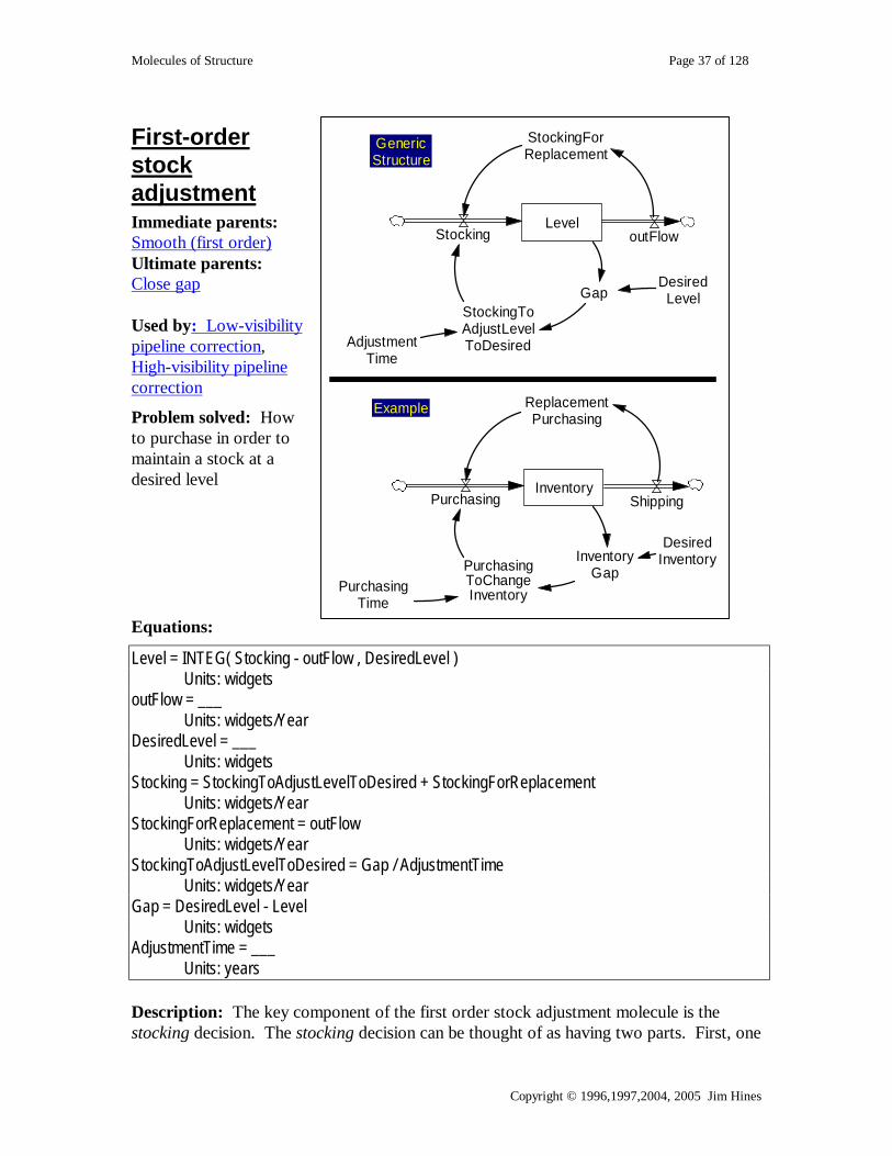
First-order stock adjustment Immediate parents: Smooth (first order) Ultimate parents: Close gap Used by: Low-visibility pipeline correction, High-visibility pipeline correction
Problem solved: How to purchase in order to maintain a stock at a desired level
Equations:
Level = INTEG( Stocking - outFlow , DesiredLevel ) Units: widgets outFlow = ___ Units: widgets/Year DesiredLevel = ___ Units: widgets Stocking = StockingToAdjustLevelToDesired + StockingForReplacement Units: widgets/Year StockingForReplacement = outFlow Units: widgets/Year StockingToAdjustLevelToDesired = Gap / AdjustmentTime Units: widgets/Year Gap = DesiredLevel - Level Units: widgets AdjustmentTime = ___ Units: years Description: The key component of the first order stock adjustment molecule is the stocking decision. The stocking decision can be thought of as having two parts. First, one
GapDesired
Level
LevelStocking outFlow
StockingToAdjustLevelToDesired
StockingForReplacement
AdjustmentTime
InventoryGap
DesiredInventory
InventoryPurchasing Shipping
PurchasingToChangeInventory
ReplacementPurchasing
PurchasingTime
GenericStructure
Example

Molecules of Structure Page 38 of 128
Copyright © 1996,1997,2004, 2005 Jim Hines
“orders” what ever is being used up (this is StockingForReplacement). This portion of the decision will keep inventories at their current levels. The second component of the decision is to “order” a bit more or a bit less to move the Level to its desired value. This decision is done in a “goal-gap” way. Structurally this molecule is a smooth with a piece added on to take care of an extra outflow from the level.
Behavior: This structure will smoothly move the actual inventory to the desired level. If the outflow were zero, this structure would be equivalent to a smooth. If the replacement part of the decision can be made immediately (as shown above) without a perception delay, the structure will behave like a smooth no matter what the outflow is.
Classic examples: A very common structure.
Caveats: In many cases the stocking flow should not go negative (e.g. if the inflow is actually a manufacturing process, one cannot “unmanufacture” what has already been placed in the level). In this case, the modeler should modify the inflow so that it cannot go negative.
This structure assumes that stocking can be made with no delay (i.e. the inflow is from off the shelf, immediately available, products). If there is a delay (e.g. the things being ordered need to be custom-made), then it may be important to consider the supply pipeline. For this see the Capacity Ordering molecule.
In some situations one may want to recognize a perception lag between the outflow and the knowledge of how much should be replaced. In this case, StockingForReplacement will should be modeled as a smooth (or perhaps an extrapolation) of the outflow.
Technical notes: None
Molecules of Structure Page 39 of 128
Copyright © 1996,1997,2004, 2005 Jim Hines
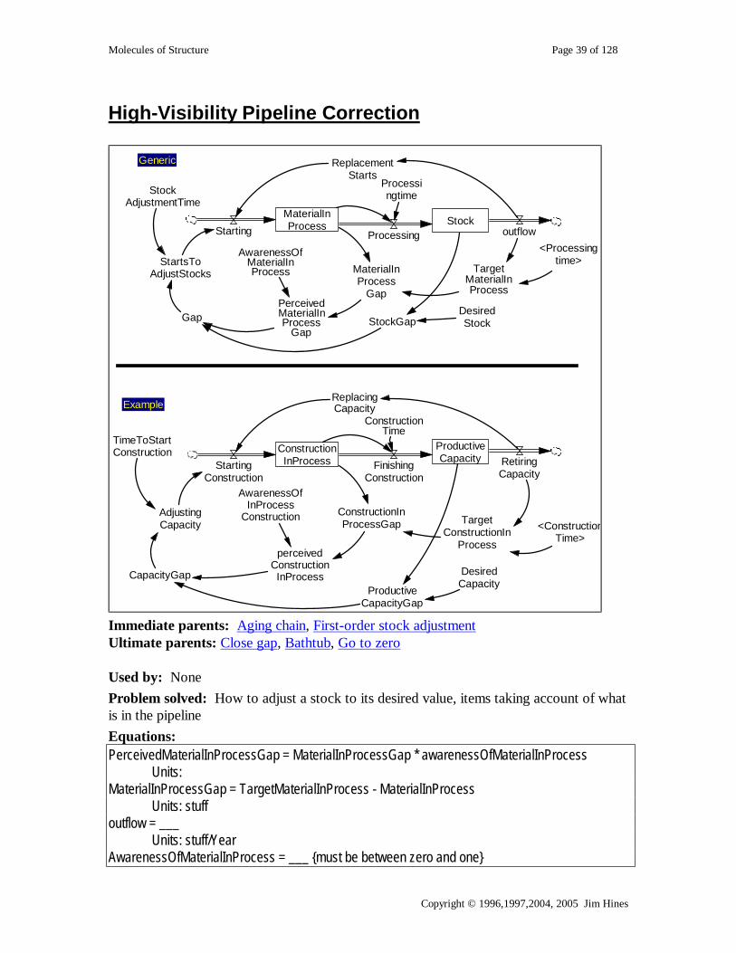
High-Visibility Pipeline Correction
ConstructionInProcess
ProductiveCapacityFinishing
Construction
ConstructionTime
StartingConstruction
RetiringCapacity
<ConstructionTime>
ProductiveCapacityGap
AwarenessOfInProcess
ConstructionAdjustingCapacity
ReplacingCapacity
TimeToStartConstruction
DesiredCapacity
TargetConstructionIn
Process
MaterialInProcess Stock
Processing
Processingtime
Starting outflow<Processing
time>
Gap
AwarenessOfMaterialInProcess
StartsToAdjustStocks
ReplacementStarts
StockAdjustmentTime
DesiredStock
TargetMaterialInProcess
StockGap
MaterialInProcess
GapPerceivedMaterialInProcess
Gap
ConstructionInProcessGap
perceivedConstructionInProcessCapacityGap
Generic
Example
Immediate parents: Aging chain, First-order stock adjustment Ultimate parents: Close gap, Bathtub, Go to zero Used by: None Problem solved: How to adjust a stock to its desired value, items taking account of what is in the pipeline Equations: PerceivedMaterialInProcessGap = MaterialInProcessGap * awarenessOfMaterialInProcess Units: MaterialInProcessGap = TargetMaterialInProcess - MaterialInProcess Units: stuff outflow = ___ Units: stuff/Year AwarenessOfMaterialInProcess = ___ {must be between zero and one}

Molecules of Structure Page 40 of 128
Copyright © 1996,1997,2004, 2005 Jim Hines
Units: fraction DesiredStock = ___ Units: stuff Stock = INTEG( Processing - outflow , DesiredStock ) Units: stuff StockGap = DesiredStock - Stock Units: stuff Processing = MaterialInProcess / Processingtime Units: stuff/Year Processingtime = ___ Units: years Gap = StockGap + PerceivedMaterialInProcessGap Units: stuff MaterialInProcess = INTEG( Starting - Processing , TargetMaterialInProcess) Units: stuff ReplacementStarts = outflow Units: stuff/Year Starting = max ( 0, StartsToAdjustStocks + ReplacementStarts ) Units: stuff/Year StartsToAdjustStocks = Gap / StockAdjustmentTime Units: stuff/Year StockAdjustmentTime = ___ Units: Year TargetMaterialInProcess = outflow * Processingtime Units: stuff Description: Based on the First-order stock adjustment structure, this molecule adds the idea that creating material is a time consuming process. As in the first-order molecule, this one also represents the need to replace what is being used (or sold) and also adjusts the stock toward a desired level. This molecule takes account not only of what is ultimately needed in the final stock, but also what is needed in the “pipe line”. Put differently, this molecule keeps track not only of what is on hand in the final stock, but also of what it has been started but has not yet been completed. The representation shown above provides a single level for in-process material, which – when combined with the final stock – results in a second-order aging chain. However, the in-process stock can easily be disaggregated simply by adding stocks to the aging chain – for example, for a production-distribution system one could have stocks of raw materials, in-process inventory, finished inventory, inventory-at-the-warehouse arranged in a fourth-order aging chain.

Molecules of Structure Page 41 of 128
Copyright © 1996,1997,2004, 2005 Jim Hines
Behavior: Failing to keep track of what is in process (i.e. failing to keep track of the “pipeline”, means that the decision for starting will over order -- it will keep ordering the same item until it is received; rather than realizing the order has been placed even though it hasn’t shown up yet. This is the main mistake that people make in playing the Beer Game. The variable awarenessOfMaterialInProcess can be set anywhere between zero and 1 to represent partial awareness of the pipeline. Failing to include replacement demand will result in steady state error.
Classic examples: Structures like this are found in Forester’s Industrial Dynamics model to represent a production-distribution system (supply chain) and in the System Dynamics National Model to represent an economy-wide aggregate structure leading from raw-materials to company’s final inventories and, ultimately, to consumer’s stocks. The structure is also used to represent construction processes for, say, office buildings or factories.
Caveats: The process of moving material from in-process to the final stage in this molecule only takes time. It does not take productivity or people. In some instances this is relatively accurate. In many instances, such as manufacturing, this is not accurate. However, the structure is still used in many such situations by the best modelers in the field, because it is simple and good enough in the sense that the dynamics of interest are not obscured.
In cases where “capacity” represents final inventory, desired inventory (i.e. “desired capacity” in the diagram) should respond to demand. If it doesn’t, the structure is at the mercy of a positive loop involving the effect of stockouts on shipments (not shown), shipments (i.e. “retiring capacity”) and ordering (i.e. “replacing capacity” and “adjusting capacity”).
Technical notes: This molecule provides a more detailed (and more specific) representation of the pipeline than the closely related Low-visibility pipeline correction molecule. This molecule is more appropriate when the decision maker has visibility of the process that “creates” the inflow into the final stock.
PIPE AWAREPIPE UNAWARECapacity
1.818 M1.614 M1.409 M1.204 M
1 M0 25 50
Time (Year)

Molecules of Structure Page 42 of 128
Copyright © 1996,1997,2004, 2005 Jim Hines
Low-visibility Pipeline Correction
Orders NotReceived
InventoryReceivingProduct
Ordering
ShippingOrder
PipelinegGap
AwarenessOfPipeline
correctionForOrdersInPipeline
ReplacementOrdering
ForecastedDemand
TimeToCorrectOrder
Pipeline
DesiredInventory
RequiredOrdersInPipeline
Orders beingfulfilled
inventoryCorrection
timeToCorrectInventory
CalculatedDeliveryDelay
Immediate parents: First-order stock adjustment, Split flow, Residence time Ultimate parents: Close gap, Bathtub Used by: None
Problem solved: How to adjust a stock to its desired value, taking into account what is in the pipeline in a situation where the decision maker does not have explicit visibility of the pipeline itself.
Equations:
Ordering = max ( 0, correctionForOrdersInPipeline + ReplacementOrdering + inventoryCorrection Units: cases/quarter ReplacementOrdering = Shipping Units: cases/quarter Shipping = ___ Units: cases/quarter inventoryCorrection = ( DesiredInventory - Inventory ) / timeToCorrectInventory

Molecules of Structure Page 43 of 128
Copyright © 1996,1997,2004, 2005 Jim Hines
Units: cases/quarter timeToCorrectInventory = ___ Units: quarter DesiredInventory = ___ Units: cases Inventory = INTEG( Receiving Product - Shipping , DesiredInventory ) Units: cases Receiving Product = ___ Units: cases/quarter correctionForOrdersInPipeline = OrderPipelinegGap / TimeToCorrectOrderPipeline Units: cases/quarter TimeToCorrectOrderPipeline = ___ Units: quarter OrderPipelinegGap = ( RequiredOrdersInPipeline - Orders Not Received ) * AwarenessOfPipeline Units: cases AwarenessOfPipeline = ___ (usually a number between between 0 and 1) Units: fraction Orders Not Received = INTEG( Ordering - Orders being fulfilled , ___) Units: cases Orders being fulfilled = Receiving Product Units: cases/quarter RequiredOrdersInPipeline = ForecastedDemand * CalculatedDeliveryDelay Units: cases CalculatedDeliveryDelay = Orders Not Received / Orders being fulfilled Units: quarters ForecastedDemand = ____ Units: cases/quarter Description: As in the First-order stock adjustment molecule, ordering has two components: replacing whatever is (expected to be) sold, and adjusting inventory. This formulation also recognizes a hidden component of inventory: Inventory that is on the way (or has been ordered), but has not yet been received. In steady state, this inventory-on-the-way will be non-zero. In fact, if the ordering rate is constant, this inventory-on-the-way will be equal to the ordering rate multiplied by the time it takes to receive orders. In other words, the inventory on the way will be the entire stream of orders that have been placed, but not received.
This structure represents a great deal of what is present at each stage of the beer game. The mistake that most beer-game players make is that they do not keep track of orders not received - they do not take account of the pipeline. In this structure this is represented by setting the Pipeline Recognition Factor to a small number. The result will be oscillations caused by placing the “same” order more than once.
Behavior: No relevant behavior because the process of incoming orders (and shipping) is not specified in this molecule.
Classic examples: This molecule is commonly used.

Molecules of Structure Page 44 of 128
Copyright © 1996,1997,2004, 2005 Jim Hines
Caveats: None
Technical notes: This molecule does not specify how an order is “processed” by a supplier. The closely related High-visibility pipeline correction molecule may be more appropriate if the decision maker has explicit knowledge of the process used to create the material.
Molecules of Structure Page 45 of 128
Copyright © 1996,1997,2004, 2005 Jim Hines
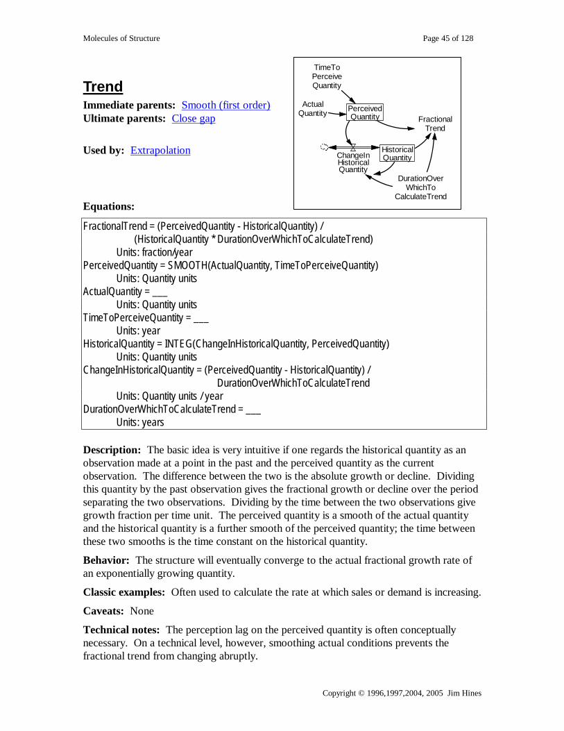
Trend Immediate parents: Smooth (first order) Ultimate parents: Close gap
Used by: Extrapolation
Equations:
FractionalTrend = (PerceivedQuantity - HistoricalQuantity) / (HistoricalQuantity * DurationOverWhichToCalculateTrend) Units: fraction/year PerceivedQuantity = SMOOTH(ActualQuantity, TimeToPerceiveQuantity) Units: Quantity units ActualQuantity = ___ Units: Quantity units TimeToPerceiveQuantity = ___ Units: year HistoricalQuantity = INTEG(ChangeInHistoricalQuantity, PerceivedQuantity) Units: Quantity units ChangeInHistoricalQuantity = (PerceivedQuantity - HistoricalQuantity) / DurationOverWhichToCalculateTrend Units: Quantity units / year DurationOverWhichToCalculateTrend = ___ Units: years Description: The basic idea is very intuitive if one regards the historical quantity as an observation made at a point in the past and the perceived quantity as the current observation. The difference between the two is the absolute growth or decline. Dividing this quantity by the past observation gives the fractional growth or decline over the period separating the two observations. Dividing by the time between the two observations give growth fraction per time unit. The perceived quantity is a smooth of the actual quantity and the historical quantity is a further smooth of the perceived quantity; the time between these two smooths is the time constant on the historical quantity.
Behavior: The structure will eventually converge to the actual fractional growth rate of an exponentially growing quantity.
Classic examples: Often used to calculate the rate at which sales or demand is increasing.
Caveats: None
Technical notes: The perception lag on the perceived quantity is often conceptually necessary. On a technical level, however, smoothing actual conditions prevents the fractional trend from changing abruptly.
HistoricalQuantityChangeIn
HistoricalQuantity
PerceivedQuantity
TimeToPerceiveQuantity
DurationOverWhichTo
CalculateTrend
FractionalTrend
ActualQuantity
Molecules of Structure Page 46 of 128
Copyright © 1996,1997,2004, 2005 Jim Hines
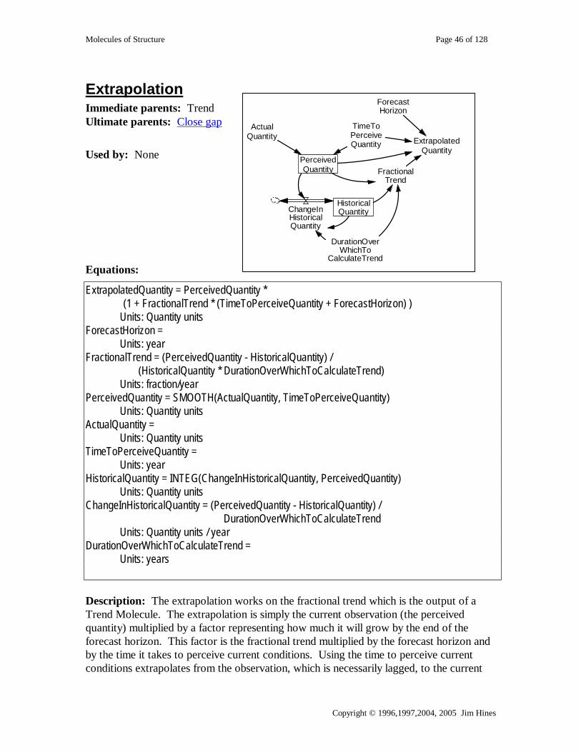
Extrapolation Immediate parents: Trend Ultimate parents: Close gap
Used by: None
Equations:
ExtrapolatedQuantity = PerceivedQuantity * (1 + FractionalTrend * (TimeToPerceiveQuantity + ForecastHorizon) ) Units: Quantity units ForecastHorizon = Units: year FractionalTrend = (PerceivedQuantity - HistoricalQuantity) / (HistoricalQuantity * DurationOverWhichToCalculateTrend) Units: fraction/year PerceivedQuantity = SMOOTH(ActualQuantity, TimeToPerceiveQuantity) Units: Quantity units ActualQuantity = Units: Quantity units TimeToPerceiveQuantity = Units: year HistoricalQuantity = INTEG(ChangeInHistoricalQuantity, PerceivedQuantity) Units: Quantity units ChangeInHistoricalQuantity = (PerceivedQuantity - HistoricalQuantity) / DurationOverWhichToCalculateTrend Units: Quantity units / year DurationOverWhichToCalculateTrend = Units: years Description: The extrapolation works on the fractional trend which is the output of a Trend Molecule. The extrapolation is simply the current observation (the perceived quantity) multiplied by a factor representing how much it will grow by the end of the forecast horizon. This factor is the fractional trend multiplied by the forecast horizon and by the time it takes to perceive current conditions. Using the time to perceive current conditions extrapolates from the observation, which is necessarily lagged, to the current
HistoricalQuantityChangeIn
HistoricalQuantity
PerceivedQuantity
TimeToPerceiveQuantity
DurationOverWhichTo
CalculateTrend
FractionalTrend
ExtrapolatedQuantity
ForecastHorizon
ActualQuantity

Molecules of Structure Page 47 of 128
Copyright © 1996,1997,2004, 2005 Jim Hines
time. Then, using the forecast horizon extrapolates from the current time to the time of the forecast horizon. However, this degree of exactness is unknown in the literature and unlikely to characterize actual trend extrapolations.
Behavior: The extrapolated forecast will be accurate for an exponentially growing quantity.
Classic examples: Extrapolations are often used to decide how much to order (or to begin construction of) in order to have the proper number of orders arriving (amount of construction coming on line) at the point in the future when we can expect our order to be filled.
Caveats: Extrapolation within an otherwise oscillatory system often will make the system more oscillatory. Note: this may be realistic.
Technical notes: What is used in the molecule is a linear extrapolation. It is roughly correct. The precise forecast would use linear extrapolation to bring the perception lag “forward” and then use continuous compounding up to the forecast horizon.

Molecules of Structure Page 48 of 128
Copyright © 1996,1997,2004, 2005 Jim Hines
Coflow There are two equivalent ways of representing a coflow. The Traditional coflow and the Hines coflow
Immediate parents: Smooth(first order) Ultimate parents: Close gap Used by: Cascaded Coflow, Coflow with Experience
Problem solved: How to keep track of a characteristic of a stock.
Equations:
Traditional Coflow avg characteristic =Characteristic/ Fundamental quantity Units: characteristic units/widget Fundamental quantity = INTEG(inflow of fundamental quantity-outflow of fundamental quantity, ___) Units: widgets inflow of fundamental quantity = ___ Units: widgets/Year outflow of fundamental quantity = ___ Units: widgets/Year Characteristic = INTEG(addl characteristic-decrease of characteristic, Fundamental quantity*characteristic of new stuff) Units: characteristic units addl characteristic = inflow of fundamental quantity*characteristic of new stuff Units: characteristic units/Year characteristic of new stuff = ___ Units: characteristic units/widget decrease of characteristic = outflow of fundamental quantity*avg characteristic Units: characteristic units/Year

Molecules of Structure Page 49 of 128
Copyright © 1996,1997,2004, 2005 Jim Hines
Hines Coflow Avg characteristic = INTEG(Change in characteristic,characteristic of new stuff,___) Units: characteristic units/widget Change in characteristic = (characteristic of new stuff-Avg characteristic)/dilution time Units: characteristic units/widget/Year characteristic of new stuff =___ Units: characteristic units/widget dilution time = Fundamental quantity/inflow of fundamental quantity Units: Year Fundamental quantity = INTEG(inflow of fundamental quantity-outflow of fundamental quantity, ___) Units: widgets inflow of fundamental quantity = ___ Units: widgets/Year outflow of fundamental quantity = ___ Units: widgets/Year Description: The Hines coflow makes clearer the relationship of coflow to smooth or Goal-Gap formulations. The traditional coflow makes clearer why it is called a “coflow”. The Hines Coflow makes clear that the characteristic is a smooth with a variable time “constant”. The dilution time determines how quickly the current characteristic will change to or be diluted by the new characteristic. The traditional coflow shows that the flows of the characteristic are linked to the flows of the fundamental quantity.
Behavior: To anticipate the behavior think of how the smooth operates.
Classic examples: A firm continually borrows money at different interest rates. The amount borrowed is the fundamental quantity. The average interest rate is the average quantity. A business continually hires people with different skill levels. The number of people is the fundamental quantity. Average amount of skill is the average characteristic.
Caveats: The outflow of the fundamental quantity has the average characteristic. In some situations this is accurate. In many situations it is accurate enough. For situations where it is not good enough, see the cascaded coflow. In the Hines coflow be careful of having the dilution time be too small relative to DT. This can happen if the fundamental quantity is (close to) zero. Be careful of divide by zero errors: In the Hines coflow a divide-by-zero will occur if the inflow of the fundamental quantity equals zero; in the Traditional coflow the divide by zero problem will occur if the fundamental quantity equals zero.
Technical notes: None

Molecules of Structure Page 50 of 128
Copyright © 1996,1997,2004, 2005 Jim Hines
Coflow with Experience There are two equivalent versions, the Traditional and the Hines.
Immediate parents: Coflow Ultimate parents: Close gap Used by: None
Problem solved: How to represent a workforce in which new people have less experience, and where everyone gains experience with time
Equations:
Traditional Coflow average experience = Total experience / Workforce Units: Years/person Workforce = INTEG( hiring - attrition , Initial Workforce ) Units: People hiring = ___ Units: People/Year attrition = Workforce / TimeToQuitOrRetire Units: People/Year Initial Workforce = INITIAL( hiring * TimeToQuitOrRetire ) Units: People TimeToQuitOrRetire = ___ Units: Year Total experience = INTEG( Add'l experience from new hires + gaining experience - experience loss , Workforce * ( average experience of new hire + rate of experience gain * Workforce / attrition ) )
Molecules of Structure Page 51 of 128
Copyright © 1996,1997,2004, 2005 Jim Hines
Units: Year experience loss = attrition * average experience Units: dmnl Add'l experience from new hires = average experience of new hire * hiring Units: dmnl average experience of new hire = ___ Units: Years/person gaining experience = Workforce * rate of experience gain Units: dmnl rate of experience gain = 1 Units: Years/(Year*person)
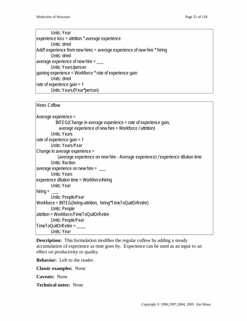
Hines Coflow Average experience = INTEG(Change in average experience + rate of experience gain, average experience of new hire + Workforce / attrition) Units: Years rate of experience gain = 1 Units: Years/Year Change in average experience = (average experience on new hire - Average experience) / experience dilution time Units: fraction average experience on new hire = ___ Units: Years experience dilution time = Workforce/hiring Units: Year hiring = ___ Units: People/Year Workforce = INTEG(hiring-attrition, hiring*TimeToQuitOrRetire) Units: People attrition = Workforce/TimeToQuitOrRetire Units: People/Year TimeToQuitOrRetire = ____ Units: Year
Description: This formulation modifies the regular coflow by adding a steady accumulation of experience as time goes by. Experience can be used as an input to an effect on productivity or quality.
Behavior: Left to the reader.
Classic examples: None
Caveats: None
Technical notes: None

Molecules of Structure Page 52 of 128
Copyright © 1996,1997,2004, 2005 Jim Hines
Cascaded Coflow Hines Cascaded Coflow
Old MaterialDilution Time
Change incharacteristicof old material Avg Characteristic
of Old Material
Maturematerial
dilution time
Change incharacteristic ofmature material Avg
characteristic ofMature material
Time to flowout
Time to age
Materialflowing out
Materialaging
Old materialMaturematerialMaterial
flowing in
Time tomature
Materialmaturing
New material
dilution time ofnew Material
Change incharacteristic
of new materialAvg characteristic new material
characteristicof new stuff
Traditional Cascaded Coflow
Old MaterialAvg
characteristic
decrease ofold material
characteristic
Old MaterialCharacteristic
MatureMaterial Avgcharacteristic
characteristictranfering frommature to old
Mature MaterialCharacteristic
Time to flowout
Time to age
Materialflowing out
Materialaging
Old materialMaturematerialMaterial
flowing in
Time tomature
Materialmaturing
New material
characteristicof new stuff
New MaterialAvg
characteristic
characteristictransfering fromnew to mature
addl newMaterial
characteristic
New MaterialCharacteristic
Immediate parents Aging chain Traditional: Traditional coflow, Broken cascade, Cascaded levels Hines: Hines coflow, Smooth (higher order) Ultimate parents: Close gap, Bathtub, Go to zero Used by: None

Molecules of Structure Page 53 of 128
Copyright © 1996,1997,2004, 2005 Jim Hines
Problem solved: How to represent a characteristic of a fundamental quantity where the outflow from the fundamental quantity is older than the average.
Equations:
Traditional Cascaded Coflow Equations Change in characteristic of old material = ( Avg characteristic of Mature material- Avg Characteristic of Old Material ) / old Material Dilution Time Units: characteristic units/(widget*Year) Avg characteristic of Mature material = INTEG( Change in characteristic of mature material, Avg characteristic new material ) Units: characteristic units/widget Avg Characteristic of Old Material = INTEG( Change in characteristic of old material, Avg characteristic of Mature material ) Units: characteristic units/widget Change in characteristic of mature material = ( Avg characteristic new material- Avg characteristic of Mature material ) / Mature material dilution time Units: characteristic units/(widget*Year) Old Material Dilution Time = Old material / Material aging Units: Year dilution time of new Material = New material / Material flowing in Units: Year Mature material dilution time = Mature material / Material maturing Units: Year Avg characteristic new material = INTEG( Change in characteristic of new material, characteristic of new stuff ) Units: characteristic units/widget Change in characteristic of new material = ( characteristic of new stuff - Avg characteristic new material ) / dilution time of new Material Units: characteristic units/(widget*Year) characteristic of new stuff = ___ Units: characteristic units/widget Material aging = Mature material / Time to age Units: stuff/Year Material flowing in = ___ Units: stuff/Year Material flowing out = Old material / Time to flow out Units: stuff/Year Material maturing = New material / Time to mature Units: stuff/Year Mature material = INTEG(Material maturing - Material aging , Material maturing * Time to age ) Units: stuff New material = INTEG(

Molecules of Structure Page 54 of 128
Copyright © 1996,1997,2004, 2005 Jim Hines
Material flowing in - Material maturing , Material flowing in * Time to mature ) Units: stuff Old material = INTEG( Material aging - Material flowing out , Material aging * Time to flow out ) Units: stuff Time to age = ___ Units: Year Time to flow out = ___ Units: years Time to mature = ___ Units: Year
Hines Cascaded Coflow Equations Avg characteristic new material = INTEG( Change in characteristic of new material, characteristic of new stuff) Units: characteristic units/widget Change in characteristic of new material = ( characteristic of new stuff - Avg characteristic new material)/dilution time of new Material Units: characteristic units/widget/Year characteristic of new stuff = ___ Units: characteristic units/widget dilution time of new Material = New material/Material flowing in Units: Year Avg characteristic of Mature material = INTEG( Change in characteristic of mature material,Avg characteristic new material) Units: characteristic units/widget Change in characteristic of mature material = (Avg characteristic new material -Avg characteristic of Mature material)/ Mature material dilution time Units: characteristic units/widget/Year Mature material dilution time = Mature material/Material maturing Units: Year Avg Characteristic of Old Material = INTEG( Change in characteristic of old material,Avg characteristic of Mature material) Units: characteristic units/widget Change in characteristic of old material = (Avg characteristic of Mature material - Avg Characteristic of Old Material)/ Old Material Dilution Time Units: characteristic units/widget/Year Old Material Dilution Time = Old material/Material aging Units: Year New material = INTEG(Material flowing in-Material maturing,Material flowing in*Time to mature) Units: stuff Material flowing in = ___ Units: stuff/Year
Molecules of Structure Page 55 of 128
Copyright © 1996,1997,2004, 2005 Jim Hines
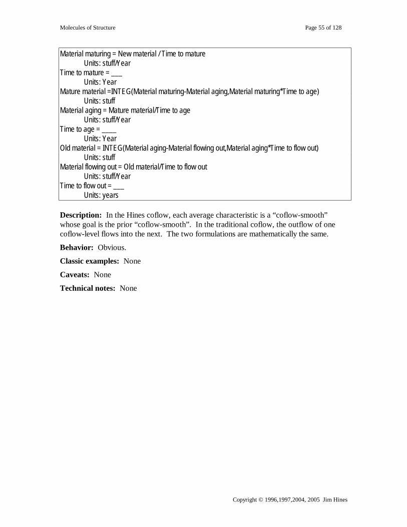
Material maturing = New material / Time to mature Units: stuff/Year Time to mature = ___ Units: Year Mature material =INTEG(Material maturing-Material aging,Material maturing*Time to age) Units: stuff Material aging = Mature material/Time to age Units: stuff/Year Time to age = ____ Units: Year Old material = INTEG(Material aging-Material flowing out,Material aging*Time to flow out) Units: stuff Material flowing out = Old material/Time to flow out Units: stuff/Year Time to flow out = ___ Units: years Description: In the Hines coflow, each average characteristic is a “coflow-smooth” whose goal is the prior “coflow-smooth”. In the traditional coflow, the outflow of one coflow-level flows into the next. The two formulations are mathematically the same.
Behavior: Obvious.
Classic examples: None
Caveats: None
Technical notes: None
Molecules of Structure Page 56 of 128
Copyright © 1996,1997,2004, 2005 Jim Hines
Dimensionless Input To Function Immediate parents: None Ultimate parents: None Used by: Univariate anchoring and adjustment
Problem solved: How to create a table function (also known as lookup function) that is easy to parameterize.
Equations:
functionOfInput = functionOfInput f(Relative Input) Units: output units functionOfInput f = [table (or “lookup”) function] Units: output units Relative Input = Input/Reference Input Units: dimensionless Input = ___ Units: Input units Reference Input = ___ Units: Input units Description: The key here is that the input to the table function is measured relative to a reference. It is usually easier for people to judge what value the function should produce for an input that is some factor of a reference, than to judge the value of the function for a raw input. The most important exception is a domain-expert who may find it easier to parameterize the function in terms of raw inputs.
The reference input is often, but not always, a constant.
Behavior: No stocks, so no endogenous behavior.
Classic examples: Effect of inventory on sales.
Caveats: Although this molecule makes it easier for a modeler who is not intimately familiar with the substantive area being modeled; this molecule can make it more difficult for the client who is extremely familiar with the subject. People with tremendous experience in a subject area may find it easier to parameter a function when the input is a raw, dimensioned quantity.
Technical notes: An added benefit of this structure is that it can be reparameterized for tuning or sensitivity testing by changing the value of the reference input (if the reference input is a constant). If the function takes raw values, the only way to reparameterize is to change (i.e. “redraw”) the function.
Input
ReferenceInput
RelativeInput
functionOfInput<functionOfInput f>

Molecules of Structure Page 57 of 128
Copyright © 1996,1997,2004, 2005 Jim Hines
Univariate Anchoring and Adjustment Immediate parents: Dimensionless input to function Ultimate parents: Dimensionless input to function Used by: Multivariate anchoring and adjustment, Nonlinear split, Level protected by level, Effect of fatigue, overtime, Level protected by pdy
Problem solved: How to model the human process of judging an “appropriate” value (e.g. actual value or ideal value) of some constant or variable. How to create a user-defined function whose equilibrium value is easy to change.
Equations:
value = Adjustment * anchor Units: valueUnits anchor = ___ Units: valueUnits Adjustment = Adjustment f ( PressureToAdjustAwayFromTheAnchor ) Units: dmnl Adjustment f ( ) = A user defined function that contains the point (1,1) Units: dmnl PressureToAdjustAwayFromTheAnchor = currentValueOfSomeVariable / normalValueOfSomeVariable Units: fraction currentValueOfSomeVariable = ___ Units: unitsOfSomeVariable normalValueOfSomeVariable = ___ Units: unitsOfSomeVariable
Description: Anchoring and Adjustment is a common judgmental strategy (Hogarth). Rather than finding a new quantity by solving a problem from scratch, people often will simply take a known quantity (the anchor) and adjust it to account for new factors or pressures. For example I don’t know the distance from London to Hamburg. So, I might start with the distance from London to Berlin (the anchor), which I happen to know. Because I know that Hamburg is closer to London than Berlin, I’ll “adjust” the value downward by “ a bit” say 20%. The structure above represents this process: A normal (or maximum or minimum) value – the “anchor” -- is multiplied (“adjusted”) by the effect (or pressure) of some piece of information. The effect has a neutral values of 1.
value
Adjustment
anchor
currentValueOfSomeVariable
normalValueOfSomeVariable
PressureToAdjustAwayFrom
TheAnchor
Adjustment f

Molecules of Structure Page 58 of 128
Copyright © 1996,1997,2004, 2005 Jim Hines
Behavior: No stocks, so no dynamics.
Classic examples: Many
Caveats: None
Technical notes: People using anchoring and adjustment in the real world often fail to adjust enough.

Molecules of Structure Page 59 of 128
Copyright © 1996,1997,2004, 2005 Jim Hines
Level Protected by Level
Level todrain
draining
Effect of level ondraining
DesiredLevel
RelativeLevel
Effect of level ondraining f
Desireddraining
Immediate parents: Univariate anchoring and adjustment Ultimate parents: Dmnl input to function
Used by: Backlog shipping protected by level
Problem solved: How to ensure that a stock does not go negative
Equations:
Level to drain = INTEG(-draining,Desired Level, ___) Units: Widgets draining = Desired draining * Effect of level on draining Units: Widgets/Month Desired draining = Units: Widgets/Month Effect of level on draining = Effect of level on draining f(Relative Level) Units: dmnl Effect of level on draining f = user defined funciton Units: dmnl Relative Level = Level to drain / Desired Level Units: dmnl Desired Level = Units: Widgets
Description: The actual outflow is the product of the desired draining and a function that shuts off the outflow as the level approaches zero. This formulation is considered much more desirable than an IF-THEN-ELSE statement both because it is less subject to integration error and, even more importantly, because it is appropriate for a stock that aggregates many items which are not identical (e.g. a finished goods inventory containing many different products and models).
Behavior: The level will not go below zero.

Molecules of Structure Page 60 of 128
Copyright © 1996,1997,2004, 2005 Jim Hines
Classic examples: Shipping out of an inventory. The inventory must not go negative.
Caveats: Watch out for functions that drop suddenly to zero, which may introduce an integration error that lets the level go slightly negative before it shuts off.
Technical notes: The table function should go through (0,0). A table function going through (1,1) will be easier to put into equilibrium. To represent probabilistic stocking out, the function should lie above the 45 degree line in the region below the point (1,1).

Molecules of Structure Page 61 of 128
Copyright © 1996,1997,2004, 2005 Jim Hines
Multivariate Anchoring and Adjustment
valueanchor
Adjustment #1
currentValueOfSomeVariable #1
normalValueOfSomeVariable #1
PressureToAdjustAwayFromThe
Anchor #1Adjustment f #1
Adjustment #2
currentValueOfSomeVariable #2
normalValueOfSomeVariable #2
PressureToAdjustAwayFromThe
Anchor #2Adjustment f #2
Adjustment #3
currentValueOfSomeVariable #3
normalValueOfSomeVariable #3PressureTo
AdjustAwayFromTheAnchor #3
Adjustment f #3
Immediate parents: Univariate anchoring and adjustment Ultimate parents: Dimensionless input To Function Used by: Productivity, Quality, Sea anchor and adjustment, Multi-dimensional split
Problem solved: How to model the human process of judging the “appropriate” value (e.g. actual value or ideal value) of some constant or variable. How to represent something that is a function of many things. How to create a function whose equilibrium value is easy to change.
Equations:
value = Anchor * "Adjustment #1" * "Adjustment #2" * "Adjustment #3" Units: cases Anchor = ___ Units: cases "Adjustment #1" = "Adjustment f #1" ( "PressureToAdjustAwayFromTheAnchor #1") Units: dmnl "Adjustment #2" = "Adjustment f #2" ( "PressureToAdjustAwayFromTheAnchor #2") Units: dmnl "Adjustment #3" = "Adjustment f #3" ( "PressureToAdjustAwayFromTheAnchor #3") Units: dmnl "Adjustment f #1" = user defined function Units: dmnl "Adjustment f #2" = user defined function Units: dmnl "Adjustment f #3" = user defined function Units: dmnl
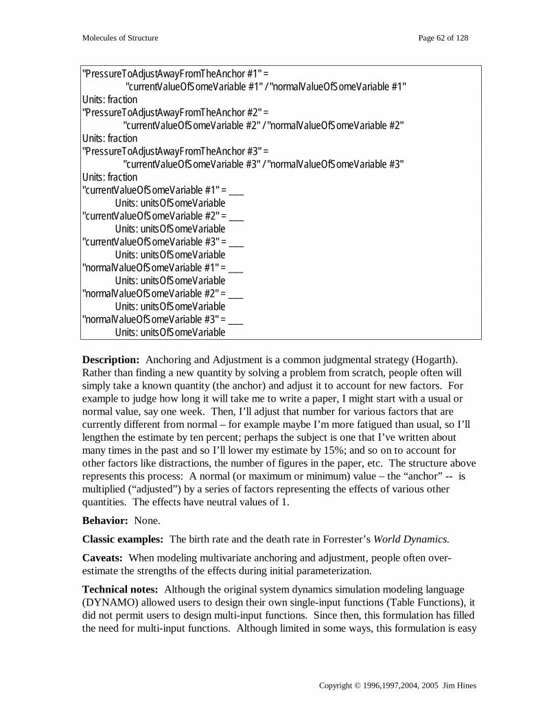
Molecules of Structure Page 62 of 128
Copyright © 1996,1997,2004, 2005 Jim Hines
"PressureToAdjustAwayFromTheAnchor #1" = "currentValueOfSomeVariable #1" / "normalValueOfSomeVariable #1" Units: fraction "PressureToAdjustAwayFromTheAnchor #2" = "currentValueOfSomeVariable #2" / "normalValueOfSomeVariable #2" Units: fraction "PressureToAdjustAwayFromTheAnchor #3" = "currentValueOfSomeVariable #3" / "normalValueOfSomeVariable #3" Units: fraction "currentValueOfSomeVariable #1" = ___ Units: unitsOfSomeVariable "currentValueOfSomeVariable #2" = ___ Units: unitsOfSomeVariable "currentValueOfSomeVariable #3" = ___ Units: unitsOfSomeVariable "normalValueOfSomeVariable #1" = ___ Units: unitsOfSomeVariable "normalValueOfSomeVariable #2" = ___ Units: unitsOfSomeVariable "normalValueOfSomeVariable #3" = ___ Units: unitsOfSomeVariable Description: Anchoring and Adjustment is a common judgmental strategy (Hogarth). Rather than finding a new quantity by solving a problem from scratch, people often will simply take a known quantity (the anchor) and adjust it to account for new factors. For example to judge how long it will take me to write a paper, I might start with a usual or normal value, say one week. Then, I’ll adjust that number for various factors that are currently different from normal – for example maybe I’m more fatigued than usual, so I’ll lengthen the estimate by ten percent; perhaps the subject is one that I’ve written about many times in the past and so I’ll lower my estimate by 15%; and so on to account for other factors like distractions, the number of figures in the paper, etc. The structure above represents this process: A normal (or maximum or minimum) value – the “anchor” -- is multiplied (“adjusted”) by a series of factors representing the effects of various other quantities. The effects have neutral values of 1.
Behavior: None.
Classic examples: The birth rate and the death rate in Forrester’s World Dynamics.
Caveats: When modeling multivariate anchoring and adjustment, people often over-estimate the strengths of the effects during initial parameterization.
Technical notes: Although the original system dynamics simulation modeling language (DYNAMO) allowed users to design their own single-input functions (Table Functions), it did not permit users to design multi-input functions. Since then, this formulation has filled the need for multi-input functions. Although limited in some ways, this formulation is easy

Molecules of Structure Page 63 of 128
Copyright © 1996,1997,2004, 2005 Jim Hines
for the modeler to visualize (a general fourth-dimensional function would be difficult) and easy to explain.

Molecules of Structure Page 64 of 128
Copyright © 1996,1997,2004, 2005 Jim Hines
Productivity (PDY) Immediate parents: Multivariate anchoring and adjustment Ultimate parents: Dmnl input to f() Used by: None
Problem solved: How to determine productivity
Equations:
Productivity = NormalProductivity * EffectOfFatigueOnProductivity * EffectOfSchedulePressureOnProductivity * EffectOfWorkAdequacyOnProductivity * EffectAverageSkillOnProductivity Units: widgets/(person*Month) AverageSkill = ___ Units: fraction EffectAverageSkillOnProductivity = EffectAverageSkillOnProductivity f ( AverageSkill) Units: dmnl EffectAverageSkillOnProductivity f = user defined function Units: dmnl NormalProductivity = ___ Units: widgets/(person*Month) EffectOfFatigueOnProductivity = EffectOfFatigueOnProductivity f ( Fatigue ) Units: dmnl EffectOfFatigueOnProductivity f = user defined function Units: dmnl Fatigue = ___ Units: fraction EffectOfSchedulePressureOnProductivity = EffectOfSchedulePressureOnProductivity f( SchedulePressure ) Units: dmnl EffectOfSchedulePressureOnProductivity f = user defined function Units: dmnl SchedulePressure = ___ Units: fraction EffectOfWorkAdequacyOnProductivity =
Productivity
NormalProductivity
EffectOfFatigueOnProductivity
EffectOfSchedulePressureOnProductivity
EffectOfWorkAdequacyOnProductivity
Fatigue SchedulePressure
WorkAdequacy
<EffectOfFatigueOn
Productivity f>
<EffectOfSchedulePressureOn
Productivity f>
<EffectWorkAdequacyOn
Productivity f>
EffectAverageSkillOn
Productivity
AverageSkill
EffectAverageSkillOn
Productivity f

Molecules of Structure Page 65 of 128
Copyright © 1996,1997,2004, 2005 Jim Hines
EffectWorkAdequacyOnProductivity f ( WorkAdequacy ) Units: dmnl EffectWorkAdequacyOnProductivity f = user defined function) Units: dmnl WorkAdequacy = ___ Units: fraction
Description: The particular effects shown above are illustrative, though common in project models. Productivity is usually defined to mean speed that a single worker (or single machine or other resource) produces. Quality (the fraction of production that is actually done correctly) is modeled separately.
Behavior: No levels, so no endogenous dynamics
Classic examples: Project models
Caveats: None
Technical notes: The first project models were developed by the consulting company Pugh Roberts. These early models used the abbreviation “PDY” for “productivity”. The same structure can be used to represent quality. Often in project models things that affect productivity also affect quality (though through different functions). An interesting effect in these formulations is the effect of schedule pressure which is usually represented as a positively sloped function for productivity (meaning more schedule pressure makes people work faster) and a negatively sloped function for quality (meaning as people work faster they make more mistakes).

Molecules of Structure Page 66 of 128
Copyright © 1996,1997,2004, 2005 Jim Hines
Quality Immediate parents: Multivariate anchoring and adjustment Ultimate parents: Dmnl input to f() Used by: None
Problem solved: How to determine quality
Equations:
Quality = min(1,NormalQuality * EffectOfFatigueOnQuality * EffectOfSchedulePressureOnQuality * EffectOfWorkAdequacyOnQuality * EffectAverageSkillOnQuality) Units: widgets/(person*Month) AverageSkill = ___ Units: fraction EffectAverageSkillOnQuality = EffectAverageSkillOnQuality f ( AverageSkill) Units: dmnl EffectAverageSkillOnQuality f = user defined function Units: dmnl NormalQuality = ___ Units: widgets/(person*Month) EffectOfFatigueOnQuality = EffectOfFatigueOnQuality f ( Fatigue ) Units: dmnl EffectOfFatigueOnQuality f = user defined function Units: dmnl Fatigue = ___ Units: fraction EffectOfSchedulePressureOnQuality = EffectOfSchedulePressureOnQuality f( SchedulePressure ) Units: dmnl EffectOfSchedulePressureOnQuality f = user defined function Units: dmnl SchedulePressure = ___ Units: fraction EffectOfWorkAdequacyOnQuality = EffectWorkAdequacyOnQuality f ( WorkAdequacy )
Quality
NormalQuality
EffectOfFatigueOnQuality
EffectOfSchedulePressureOn
Quality
EffectOfWorkAdequacyOn
Quality
Fatigue SchedulePressure
WorkAdequacy
EffectOfFatigueOnQuality f
EffectOfSchedulePressureOn
Quality f
EffectWorkAdequacyOn
Quality f
EffectAverageSkillOnQuality
AverageSkill
EffectAverageSkillOnQuality f

Molecules of Structure Page 67 of 128
Copyright © 1996,1997,2004, 2005 Jim Hines
Units: dmnl EffectWorkAdequacyOnQuality f = user defined function) Units: dmnl WorkAdequacy = ___ Units: fraction Description: The particular effects shown above are illustrative, though common in project models. Quality is defined as the fraction of work that is being done correctly. In project models, productivity – meaning the speed with which work gets done (whether or not its correctly done -- is defined separately from quality.
Behavior: No levels, so no endogenous dynamics
Classic examples: Project models
Caveats: Quality should not go above 1 or below 0. Usually the table functions won’t go below zero, but they may go above one. Consequently, the result of multiplying normal quality by all the table functions could be a number greater than one. The use of the MIN function as shown in the equation for quality is a common solution to this risk.
Technical notes: The same structure can be used to represent productivity. Often in project models things that affect quality also affect productivity (though through different functions). An interesting item in these formulations is the effect of schedule pressure which is usually represented as a positively sloped function for productivity (meaning more schedule pressure makes people work faster) and as a negatively sloped function for quality (meaning as people work faster they make more mistakes).

Molecules of Structure Page 68 of 128
Copyright © 1996,1997,2004, 2005 Jim Hines
Sea Anchor and Adjustment
AnchorChangeInAnchor
Time to changeanchor
InitialAnchor value
Adjustment#1
currentValueOfSomeVariable #1
normalValueOfSomeVariable #1
PressureToAdjustAwayFromTheAnchor #1
Adjustment f#1
Adjustment#2
currentValueOfSomeVariable #2
normalValueOfSomeVariable #2
PressureToAdjustAwayFromTheAnchor #2
Adjustment f#2
Adjustment#3
currentValueOfSomeVariable #3
normalValueOfSomeVariable #3
PressureToAdjustAwayFromTheAnchor #3
Adjustment f #3
Immediate parents: Multivariate anchoring and adjustment, Smooth (first order) Ultimate parents: Dimensionless input to function, Close gap
Used by: Protected sea anchoring and adjustment, Sea anchor pricing
Problem solved: How to represent a process by which people will “grope” toward a proper quantity. How to form the anchor in an Anchoring and Adjustment process.
Equations:
value = Anchor * "Adjustment #1" * "Adjustment #2" * "Adjustment #3" Units: cases Anchor = INTEG( ChangeInAnchor , InitialAnchor ) Units: cases InitialAnchor = ___ Units: cases ChangeInAnchor = ( value - Anchor ) / Time to change anchor Units: cases/Month Time to change anchor = ___ Units: Month "Adjustment #1" = "Adjustment f #1" ( "PressureToAdjustAwayFromTheAnchor #1") Units: dmnl "Adjustment #2" = "Adjustment f #2" ( "PressureToAdjustAwayFromTheAnchor #2")

Molecules of Structure Page 69 of 128
Copyright © 1996,1997,2004, 2005 Jim Hines
Units: dmnl "Adjustment #3" = "Adjustment f #3" ( "PressureToAdjustAwayFromTheAnchor #3") Units: dmnl "Adjustment f #1" = user defined function Units: dmnl "Adjustment f #2" = user defined function Units: dmnl "Adjustment f #3" = user defined function Units: dmnl "PressureToAdjustAwayFromTheAnchor #1" = "currentValueOfSomeVariable #1" / "normalValueOfSomeVariable #1" Units: fraction "PressureToAdjustAwayFromTheAnchor #2" = "currentValueOfSomeVariable #2" / "normalValueOfSomeVariable #2" Units: fraction "PressureToAdjustAwayFromTheAnchor #3" = "currentValueOfSomeVariable #3" / "normalValueOfSomeVariable #3" Units: fraction "currentValueOfSomeVariable #1" = ___ Units: unitsOfSomeVariable "currentValueOfSomeVariable #2" = ___ Units: unitsOfSomeVariable "currentValueOfSomeVariable #3" = ___ Units: unitsOfSomeVariable "normalValueOfSomeVariable #1" = ___ Units: unitsOfSomeVariable "normalValueOfSomeVariable #2" = ___ Units: unitsOfSomeVariable "normalValueOfSomeVariable #3" = ___ Units: unitsOfSomeVariable
Description: This is an elaboration on the judgmental strategy known as anchoring and adjustment. In anchoring and adjustment a judgment is made (or a quantity) by taking an underlying quantity (an anchor) and adjusting it on the basis of current information or pressures. This formulation contains the added idea that the anchor is formed on the bases of the past judgments.
Behavior: A positive pressure will cause the quantity to immediately jump above the anchor. In the pressure persists, the quantity will begin to rise as the anchor does. If the pressure drops, the quantity will again respond immediately.
Classic examples: Anchor Pricing.
Caveats: This structure will get stuck at zero if the anchor becomes zero. To solve this use the protected sea anchoring and adjustment molecule.
Technical notes: Note there are two kinds of “parameters” to set: the adjustment time and the user function (s).

Molecules of Structure Page 70 of 128
Copyright © 1996,1997,2004, 2005 Jim Hines
Protected Sea Anchoring and Adjustment
AnchorChangeInAnchorTime to change
anchor
InitialAnchor
minimumanchorTarget
Anchor
value
Adjustment #1
currentValueOfSomeVariable #1
normalValueOfSomeVariable #1 PressureToAdjustAway
FromTheAnchor #1
Adjustment f #1Adjustment #2
currentValueOfSomeVariable #2
normalValueOfSomeVariable #2
PressureToAdjustAwayFromTheAnchor #2
Adjustment f #2Adjustment #3
currentValueOfSomeVariable #3
normalValueOfSomeVariable #3
PressureToAdjustAwayFromTheAnchor #3
Adjustment f #3
Immediate parents: Sea anchor and adjustment Ultimate parents: Dimensionless input to function
Used by: Protected Anchor Pricing
Problem solved: Represent a judgmental strategy that will grope toward a solution, and which will not get “stuck” at zero.
Equations:
value = Anchor * "Adjustment #1" * "Adjustment #2" * "Adjustment #3" Units: cases Anchor = INTEG( ChangeInAnchor , InitialAnchor ) Units: cases InitialAnchor = ___ Units: cases ChangeInAnchor = ( Target Anchor - Anchor ) / Time to change anchor Units: cases/MonthTime to change anchor = ___

Molecules of Structure Page 71 of 128
Copyright © 1996,1997,2004, 2005 Jim Hines
Units: Month Target Anchor = MAX ( value , minimum anchor ) Units: cases minimum anchor = ___ Units: cases "Adjustment #1" = "Adjustment f #1" ( "PressureToAdjustAwayFromTheAnchor #1") Units: dmnl "Adjustment #2" = "Adjustment f #2" ( "PressureToAdjustAwayFromTheAnchor #2") Units: dmnl "Adjustment #3" = "Adjustment f #3" ( "PressureToAdjustAwayFromTheAnchor #3") Units: dmnl "Adjustment f #1" = user defined function Units: dmnl "Adjustment f #2" = user defined function Units: dmnl "Adjustment f #3" = user defined function Units: dmnl "PressureToAdjustAwayFromTheAnchor #1" = "currentValueOfSomeVariable #1" / "normalValueOfSomeVariable #1" Units: fraction "PressureToAdjustAwayFromTheAnchor #2" = "currentValueOfSomeVariable #2" / "normalValueOfSomeVariable #2" Units: fraction "PressureToAdjustAwayFromTheAnchor #3" = "currentValueOfSomeVariable #3" / "normalValueOfSomeVariable #3" Units: fraction "currentValueOfSomeVariable #1" = ___ Units: unitsOfSomeVariable "currentValueOfSomeVariable #2" = ___ Units: unitsOfSomeVariable "currentValueOfSomeVariable #3" = ___ Units: unitsOfSomeVariable "normalValueOfSomeVariable #1" = ___ Units: unitsOfSomeVariable "normalValueOfSomeVariable #2" = ___ Units: unitsOfSomeVariable "normalValueOfSomeVariable #3" = ___ Units: unitsOfSomeVariable
Description: This molecule adds to its parent, Anchoring and Adjustment, a Target Anchor. The Target Anchor is the maximum of either the quantity itself or the smallest value that the anchor should take on.
Behavior: Similar to Anchoring and Adjustment, except it will not get stuck at zero (as long as the minimum anchor is greater than zero.
Classic examples: Protected sea anchor pricing

Molecules of Structure Page 72 of 128
Copyright © 1996,1997,2004, 2005 Jim Hines
Caveats: None
Technical notes: The minimum anchor should be set above zero to ensure that this formulation will not get stuck at zero. There are two kinds of parameters that determine the dynamics the time constant and the user-defined functions.

Molecules of Structure Page 73 of 128
Copyright © 1996,1997,2004, 2005 Jim Hines
Sea Anchor Pricing
UnderlyingPrice
ChangeInUnderlyingPrice
Price
Time to changeunderlying price
TimeToChangeUnderlyingMargin
UnderlyingMargin
ChangeInUnderlying
Margin
MarginPrice.
cost
RelativeInventory
EffectOfInventoryOn
Price
Inventory
TargetInventory
RelativeMarketShare
EffectOfMarketShareOnPrice
MarketShare
targetMarketShare
EffectOfInventoryOn
Price f
EffectOfMarketShareOnPrice f
RelativeInventory.
EffectOfInventoryOnMargin
Inventory.
TargetInventory.
RelativeMarketShare.
EffectOfMarketShareOnMargin
MarketShare.
targetMarketShare.
EffectOfInventoryOn
Margin f
EffectOfMarketShareOnMargin f
pressureToChangePrice
pressureToChangeMargin
Immediate parents: Sea Anchoring and Adjustment Ultimate parents: Dmnl input to function, Close gap
Used by: Protected sea anchor pricing, Smooth pricing
Problem solved: How to formulate price setting
Equations: Equations for price form Price = UnderlyingPrice * pressureToChangePrice Units: $/widget UnderlyingPrice = INTEG(ChangeInUnderlyingPrice, ___) Units: $/widget ChangeInUnderlyingPrice =( Price - UnderlyingPrice) /Time to change underlying price Units: $/widget/year Time to change underlying price = ___ Units: year pressureToChangePrice = EffectOfInventoryOnPrice * EffectOfMarketShareOnPrice Units: dmnl EffectOfInventoryOnPrice = EffectOfInventoryOnPrice f(RelativeInventory) Units: dmnl

Molecules of Structure Page 74 of 128
Copyright © 1996,1997,2004, 2005 Jim Hines
EffectOfInventoryOnPrice f = user defined function Units: dmnl EffectOfMarketShareOnPrice = EffectOfMarketShareOnPrice f(RelativeMarketShare) Units: dmnl EffectOfMarketShareOnPrice f = user defined function Units: dmnl Equations for margin form "Price." = cost * Margin Units: $/widget cost = ___ Units: $/widget Margin = UnderlyingMargin * pressureToChangeMargin Units: fraction UnderlyingMargin = INTEG( ChangeInUnderlyingMargin , ___) Units: fraction ChangeInUnderlyingMargin = ( Margin - UnderlyingMargin ) / TimeToChangeUnderlyingMargin Units: fraction/year TimeToChangeUnderlyingMargin = ___ Units: year pressureToChangeMargin = EffectOfInventoryOnMargin * EffectOfMarketShareOnMargin Units: dmnl EffectOfInventoryOnMargin = EffectOfInventoryOnMargin f ( "RelativeInventory." ) Units: dmnl EffectOfInventoryOnMargin f = user defined function Units: dmnl EffectOfMarketShareOnMargin = EffectOfMarketShareOnMargin f ( "RelativeMarketShare." ) Units: dmnl EffectOfMarketShareOnMargin f = user defined function Units: dmnl Equations common to both the “price” and the “margin” forms RelativeInventory = Inventory / TargetInventory Units: fraction TargetInventory = ___ Units: widgets Inventory = ___ Units: widgets RelativeMarketShare = MarketShare / targetMarketShare Units: fraction targetMarketShare = ___ Units: $/widget MarketShare = ___
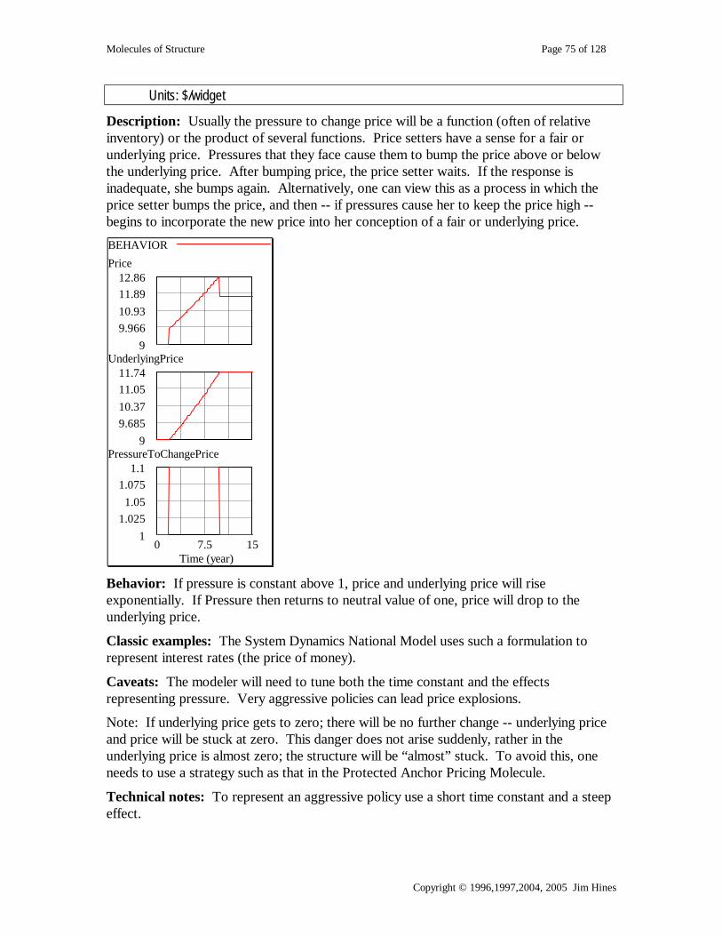
Molecules of Structure Page 75 of 128
Copyright © 1996,1997,2004, 2005 Jim Hines
Units: $/widget
Description: Usually the pressure to change price will be a function (often of relative inventory) or the product of several functions. Price setters have a sense for a fair or underlying price. Pressures that they face cause them to bump the price above or below the underlying price. After bumping price, the price setter waits. If the response is inadequate, she bumps again. Alternatively, one can view this as a process in which the price setter bumps the price, and then -- if pressures cause her to keep the price high -- begins to incorporate the new price into her conception of a fair or underlying price. BEHAVIORPrice
12.8611.8910.939.966
9UnderlyingPrice
11.7411.0510.379.685
9PressureToChangePrice
1.11.075
1.051.025
10 7.5 15
Time (year) Behavior: If pressure is constant above 1, price and underlying price will rise exponentially. If Pressure then returns to neutral value of one, price will drop to the underlying price.
Classic examples: The System Dynamics National Model uses such a formulation to represent interest rates (the price of money).
Caveats: The modeler will need to tune both the time constant and the effects representing pressure. Very aggressive policies can lead price explosions.
Note: If underlying price gets to zero; there will be no further change -- underlying price and price will be stuck at zero. This danger does not arise suddenly, rather in the underlying price is almost zero; the structure will be “almost” stuck. To avoid this, one needs to use a strategy such as that in the Protected Anchor Pricing Molecule.
Technical notes: To represent an aggressive policy use a short time constant and a steep effect.

Molecules of Structure Page 76 of 128
Copyright © 1996,1997,2004, 2005 Jim Hines
Protected Sea Anchor Pricing
MinimumUnderlyingPrice
IndicatedUnderlying
Price
UnderlyingPrice
ChangeInUnderlying
Price
Price
Time to changeunderlying
price
RelativeInventory
EffectOfInventoryOn
Price
Inventory
TargetInventory
RelativeMarketShare
EffectOfMarketShare
OnPrice
MarketShare
targetMarketShare
EffectOfInventoryOn
Price f
EffectOfMarketShare
OnPrice fpressureToChangePrice
Immediate parents: Protected sea anchoring and adjustment, Sea anchor pricing Ultimate parents: Dmnl input to function, Close gap
Used by: None
Problem solved: How to represent pricing when the price can take on a value of (or close to) zero.
Equations:
Price = UnderlyingPrice * pressureToChangePrice Units: $/widget UnderlyingPrice = INTEG(ChangeInUnderlyingPrice, ___) Units: $/widget ChangeInUnderlyingPrice = ( IndicatedUnderlyingPrice - UnderlyingPrice) /Time to change underlying price Units: $/widget/year Time to change underlying price = ___ Units: year IndicatedUnderlyingPrice = MAX(Price, MinimumUnderlyingPrice) Units: $/widget MinimuUnderlyingPrice = ___ Units: $/widget pressureToChangePrice = EffectOfInventoryOnPrice * EffectOfMarketShareOnPrice

Molecules of Structure Page 77 of 128
Copyright © 1996,1997,2004, 2005 Jim Hines
Units: dmnl EffectOfInventoryOnPrice = EffectOfInventoryOnPrice f(RelativeInventory) Units: dmnl EffectOfInventoryOnPrice f = user defined function Units: dmnl EffectOfMarketShareOnPrice = EffectOfMarketShareOnPrice f(RelativeMarketShare) Units: dmnl EffectOfMarketShareOnPrice f = user defined function Units: dmnl RelativeInventory = Inventory / TargetInventory Units: fraction TargetInventory = ___ Units: widgets Inventory = ___ Units: widgets RelativeMarketShare = MarketShare / targetMarketShare Units: fraction targetMarketShare = ___ Units: $/widget MarketShare = ___ Units: $/widget
Description: This molecule adds to the Sea Anchor Pricing Molecule the idea of a minimum underlying price. The minimum underlying price represents what pricers regard as the lowest fair or sustainable price. This might be the cost of the product.
Behavior: Same as Anchor Pricing, but the underlying price will not go below the minimum.
Classic examples: National Model uses this formulation for the interest rate, the price of money
Caveats: See Protected sea anchor and adjustment and Sea anchor pricing
Technical notes: See Protected sea anchor and adjustment and Sea anchor pricing

Molecules of Structure Page 78 of 128
Copyright © 1996,1997,2004, 2005 Jim Hines
Smooth Pricing
Pricechanging
Price
IndicatedPrice
Time to changeprice
Initial Price
RelativeInventory
EffectOfInventoryOnPrice
Inventory
TargetInventory
RelativeMarketShare
EffectOfMarket
ShareOnPrice
MarketShare
targetMarketShare
EffectOfInventoryOn
Price f
EffectOfMarketShare
OnPrice fpressureToChangePrice
Immediate parents: Sea anchor pricing Ultimate parents: Dmnl input to function, Close gap
Used by: None
Problem solved: How to represent price setting behavior where price does not change suddenly.
Equations:
Price = INTEG(changingPrice, InitialPrice) Units: $/widget InitialPrice = ___ Units: $/widget changingPrice =( IndicatedPrice - UnderlyingPrice) /Time to change underlying price Units: $/widget/year Time to change underlying price = ___ Units: year IndicatedPrice = UnderlyingPrice * pressureToChangePrice Units: $/widget pressureToChangePrice = EffectOfInventoryOnPrice * EffectOfMarketShareOnPrice Units: dmnl EffectOfInventoryOnPrice = EffectOfInventoryOnPrice f(RelativeInventory) Units: dmnl EffectOfInventoryOnPrice f = user defined function Units: dmnl

Molecules of Structure Page 79 of 128
Copyright © 1996,1997,2004, 2005 Jim Hines
EffectOfMarketShareOnPrice = EffectOfMarketShareOnPrice f(RelativeMarketShare) Units: dmnl EffectOfMarketShareOnPrice f = user defined function Units: dmnl RelativeInventory = Inventory / TargetInventory Units: fraction TargetInventory = ___ Units: widgets Inventory = ___ Units: widgets RelativeMarketShare = MarketShare / targetMarketShare Units: fraction targetMarketShare = ___ Units: $/widget MarketShare = ___ Units: $/widget
Description: In this version of price setting, the anchor is price itself which smooths to the indicated price.
Behavior: Price rises exponentially as long as the pressure to adjust is greater than one. It stops adjusting when pressure returns to 1. Note that price is “sluggish” in that it cannot react immediately to changes in pressure, unlike the case for the otherwise similar Anchor Pricing Molecule.
Classic examples: None
Caveats: At a price of zero, the structure gets “stuck”. Further at a price of almost zero, the structure will almost be stuck.
Technical notes: The speed with which price changes depends on both the functions and on the adjustment time.
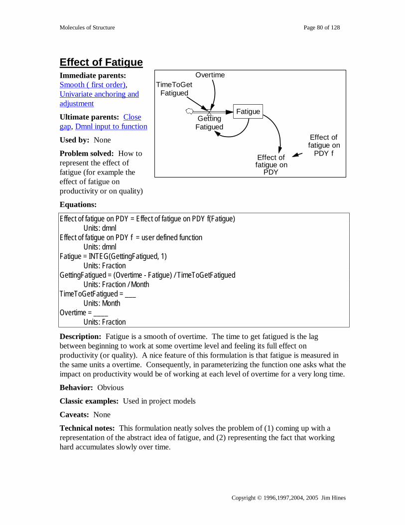
Molecules of Structure Page 80 of 128
Copyright © 1996,1997,2004, 2005 Jim Hines
Effect of Fatigue Immediate parents: Smooth ( first order), Univariate anchoring and adjustment
Ultimate parents: Close gap, Dmnl input to function
Used by: None
Problem solved: How to represent the effect of fatigue (for example the effect of fatigue on productivity or on quality)
Equations:
Effect of fatigue on PDY = Effect of fatigue on PDY f(Fatigue) Units: dmnl Effect of fatigue on PDY f = user defined function Units: dmnl Fatigue = INTEG(GettingFatigued, 1) Units: Fraction GettingFatigued = (Overtime - Fatigue) / TimeToGetFatigued Units: Fraction / Month TimeToGetFatigued = ___ Units: Month Overtime = ____ Units: Fraction
Description: Fatigue is a smooth of overtime. The time to get fatigued is the lag between beginning to work at some overtime level and feeling its full effect on productivity (or quality). A nice feature of this formulation is that fatigue is measured in the same units a overtime. Consequently, in parameterizing the function one asks what the impact on productivity would be of working at each level of overtime for a very long time.
Behavior: Obvious
Classic examples: Used in project models
Caveats: None
Technical notes: This formulation neatly solves the problem of (1) coming up with a representation of the abstract idea of fatigue, and (2) representing the fact that working hard accumulates slowly over time.
FatigueGetting
Fatigued
TimeToGetFatigued
Overtime
Effect offatigue on
PDY
Effect offatigue on
PDY f
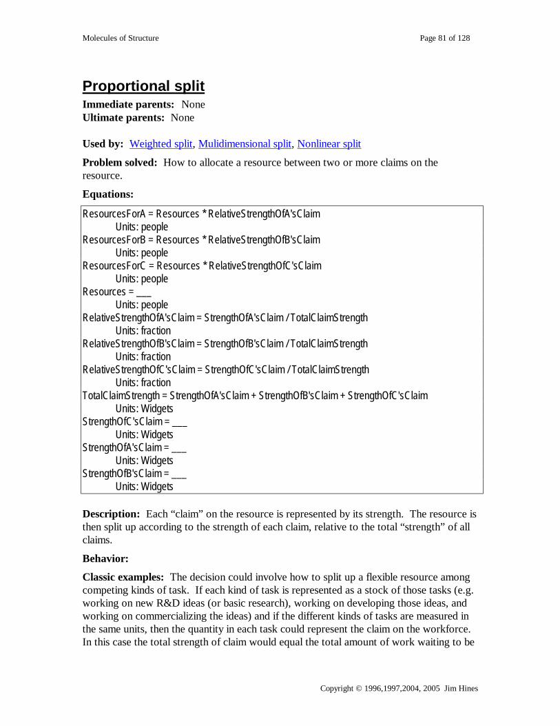
Molecules of Structure Page 81 of 128
Copyright © 1996,1997,2004, 2005 Jim Hines
Proportional split Immediate parents: None Ultimate parents: None Used by: Weighted split, Mulidimensional split, Nonlinear split
Problem solved: How to allocate a resource between two or more claims on the resource.
Equations:
ResourcesForA = Resources * RelativeStrengthOfA'sClaim Units: people ResourcesForB = Resources * RelativeStrengthOfB'sClaim Units: people ResourcesForC = Resources * RelativeStrengthOfC'sClaim Units: people Resources = ___ Units: people RelativeStrengthOfA'sClaim = StrengthOfA'sClaim / TotalClaimStrength Units: fraction RelativeStrengthOfB'sClaim = StrengthOfB'sClaim / TotalClaimStrength Units: fraction RelativeStrengthOfC'sClaim = StrengthOfC'sClaim / TotalClaimStrength Units: fraction TotalClaimStrength = StrengthOfA'sClaim + StrengthOfB'sClaim + StrengthOfC'sClaim Units: Widgets StrengthOfC'sClaim = ___ Units: Widgets StrengthOfA'sClaim = ___ Units: Widgets StrengthOfB'sClaim = ___ Units: Widgets Description: Each “claim” on the resource is represented by its strength. The resource is then split up according to the strength of each claim, relative to the total “strength” of all claims.
Behavior:
Classic examples: The decision could involve how to split up a flexible resource among competing kinds of task. If each kind of task is represented as a stock of those tasks (e.g. working on new R&D ideas (or basic research), working on developing those ideas, and working on commercializing the ideas) and if the different kinds of tasks are measured in the same units, then the quantity in each task could represent the claim on the workforce. In this case the total strength of claim would equal the total amount of work waiting to be

Molecules of Structure Page 82 of 128
Copyright © 1996,1997,2004, 2005 Jim Hines
done. Alternatively, each claim could be the amount of workers that each area in the R&D chain requests. In this case the total strength of claim would also be the total number of people requested.
Caveats: This formulation will allocate all of the resource even if that means that more resources are allocated to a particular area than are needed. Additional structure and careful thought is required to re-allocate any excesses from one claim to another.
Technical notes: None

Molecules of Structure Page 83 of 128
Copyright © 1996,1997,2004, 2005 Jim Hines
Weighted Split Immediate parents: Proportional split Ultimate parents: Proportional split Used by: None
Problem solved: How to represent managerial preferences (or bias) in an allocation decision
Equations:
resourcesForA = Resources * RelativeStrengthOfA'sClaim Units: people ResourcesForB = Resources * RelativeStrengthOfB'sClaim Units: people ResourcesForC = Resources * RelativeStrengthOfC'sClaim Units: people Resources = ___ Units: people RelativeStrengthOfA'sClaim = WeightedStrengthOfA'sClaim / TotalClaimStrength Units: fraction RelativeStrengthOfB'sClaim = WeightedStrengthOfB'sClaim / TotalClaimStrength Units: fraction RelativeStrengthOfC'sClaim = WeightedStrengthOfC'sClaim / TotalClaimStrength Units: fraction TotalClaimStrength = WeightedStrengthOfA'sClaim + WeightedStrengthOfB'sClaim + WeightedStrengthOfC'sClaim Units: Widgets WeightedStrengthOfA'sClaim = StrengthOfA'sClaim * WeightForA Units: Widgets WeightedStrengthOfB'sClaim = StrengthOfB'sClaim * WeightForB Units: Widgtets WeightedStrengthOfC'sClaim = StrengthOfC'sClaim * WeightForC Units: Widgets StrengthOfA'sClaim = ___ Units: Widgets StrengthOfB'sClaim = ___
Resources
RelativeStrengthOfA'sClaim
resourcesForA
StrengthOfA'sClaim
StrengthOfB'sClaim
TotalClaimStrength
ResourcesForB
StrengthOfC'sClaim
RelativeStrengthOfB'sClaim
RelativeStrengthOfC'sClaim
ResourcesForC
WeightedStrengthOfA'sClaim
WeightedStrengthOfB'sClaim
WeightedStrengthOfC'sClaim
WeightForA Weight
ForB
WeightForC
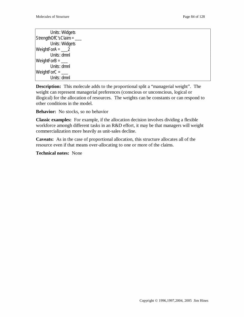
Molecules of Structure Page 84 of 128
Copyright © 1996,1997,2004, 2005 Jim Hines
Units: Widgets StrengthOfC'sClaim = ___ Units: Widgets WeightForA = ___2 Units: dmnl WeightForB = ___ Units: dmnl WeightForC = ___ Units: dmnl
Description: This molecule adds to the proportional split a “managerial weight”. The weight can represent managerial preferences (conscious or unconscious, logical or illogical) for the allocation of resources. The weights can be constants or can respond to other conditions in the model.
Behavior: No stocks, so no behavior
Classic examples: For example, if the allocation decision involves dividing a flexible workforce amongh different tasks in an R&D effort, it may be that managers will weight commercialization more heavily as unit-sales decline.
Caveats: As in the case of proportional allocation, this structure allocates all of the resource even if that means over-allocating to one or more of the claims.
Technical notes: None

Molecules of Structure Page 85 of 128
Copyright © 1996,1997,2004, 2005 Jim Hines
Multidimensional Split
EffectOfFactorAOnStrengthOf
Claim f
EffectOfFactorBOnStrengthOf
Claim f
FractionFor 2
TotalStrengthOfClaim
FractionFor 1 Fraction
For 3
StrengthOfClaim-1
EffectOfFactorBOnStrengthOf
Claim-1
EffectOffactorAOnStrengthOf
Claim-1
FactorA-1
RelativeFactorB-1
FactorB-1
NormalFactorB
StrengthOfClaim-2
EffectOfFactorBOnStrengthOf
Claim-2
EffectOfFactorAOnStrengthOf
Claim-2
factorA-2
RelativeFactorB-2
FactorB-2
StrengthOfClaim-3
EffectOfFactorBOnStrengthOf
Claim-3
EffectOfFactorAOnStrengthOf
Claim-3
factorA-3
RelativeFactorB-3 Factor
B-3
<EffectOfFactorAOnStrengthOf
Claim f>
<EffectOfFactorBOnStrengthOf
Claim f>
<EffectOfFactorAOnStrengthOf
Claim f>
<EffectOfFactorBOnStrengthOf
Claim f>
<NormalFactorB>
<NormalFactorB>
RelativeFactorA-1
RelativeFactorA-2
RelativeFactorA-3
normalFactorA
<normalFactorA>
<normalFactorA>
Quantity
QuantityFor 1
QuantityFor 2 Quantity
For 3
Immediate parents: Multivariate anchoring and adjustment, Proportional split Ultimate parents: Dmnl input to function, Proportional split Used by: Market share
Problem solved: How to allocate a resource when the strength of each claim is determined by a number of factors.
Equations:
QuantityFor 1 = Quantity * FractionFor 1 Units: stuff QuantityFor 2 = Quantity * FractionFor 2 Units: stuff QuantityFor 3 = Quantity * FractionFor 3 Units: stuff Quantity = ____ Units: stuff FractionFor 1 = "StrengthOfClaim-1" / TotalStrengthOfClaim Units: fraction FractionFor 2 = "StrengthOfClaim-2" / TotalStrengthOfClaim Units: fraction FractionFor 3 = "StrengthOfClaim-3" / TotalStrengthOfClaim Units: fraction

Molecules of Structure Page 86 of 128
Copyright © 1996,1997,2004, 2005 Jim Hines
TotalStrengthOfClaim = "StrengthOfClaim-1" + "StrengthOfClaim-2" + "StrengthOfClaim-3" Units: dmnl "StrengthOfClaim-1" = "EffectOffactorAOnStrengthOfClaim-1" * “EffectOfFactorBOnStrengthOfClaim-1" Units: dmnl "StrengthOfClaim-2" = "EffectOfFactorAOnStrengthOfClaim-2" * "EffectOfFactorBOnStrengthOfClaim-2" Units: dmnl "StrengthOfClaim-3" = "EffectOfFactorAOnStrengthOfClaim-3" * "EffectOfFactorBOnStrengthOfClaim-3" Units: dmnl "EffectOffactorAOnStrengthOfClaim-1" = EffectOfFactorAOnStrengthOfClaim f ( "RelativeFactorA-1" )
Units: dmnl EffectOfFactorAOnStrengthOfClaim f = user defined function Units: dmnl "RelativeFactorA-1" = "FactorA-1" / normalFactorA Units: fraction normalFactorA = ___ Units: FactorAUnits "FactorA-1" = ___ Units: FactorAUnits "EffectOfFactorBOnStrengthOfClaim-1" = EffectOfFactorBOnStrengthOfClaim f ( "RelativeFactorB-1") Units: dmnl "RelativeFactorB-1" = "FactorB-1" / NormalFactorB Units: fraction NormalFactorB = ___ Units: FactorBUnits "FactorB-1" = ___ Units: FactorBUnits EffectOfFactorBOnStrengthOfClaim f = user defnined function Units: dmnl "EffectOfFactorAOnStrengthOfClaim-2" = EffectOfFactorAOnStrengthOfClaim f ( "RelativeFactorA-2") Units: dmnl "RelativeFactorA-2" = "factorA-2" / normalFactorA Units: fraction "factorA-2" = ___ Units: FactorAUnits "EffectOfFactorBOnStrengthOfClaim-2" = EffectOfFactorBOnStrengthOfClaim f ( "RelativeFactorB-2") Units: dmnl "RelativeFactorB-2" = "FactorB-2" / NormalFactorB

Molecules of Structure Page 87 of 128
Copyright © 1996,1997,2004, 2005 Jim Hines
Units: fraction "FactorB-2" = ___ Units: FactorBUnits "EffectOfFactorAOnStrengthOfClaim-3" = EffectOfFactorAOnStrengthOfClaim f ( "RelativeFactorA-3") Units: dmnl "RelativeFactorA-3" = "factorA-3" / normalFactorA Units: fraction "factorA-3" = ___ Units: FactorAUnits "EffectOfFactorBOnStrengthOfClaim-3" = EffectOfFactorBOnStrengthOfClaim f ( "RelativeFactorB-3") Units: dmnl "RelativeFactorB-3" = "FactorB-3" / NormalFactorB Units: fraction "FactorB-3" = ___ Units: FactorBUnits
Description: This molecule adds to the proportional split molecule a definition for claims based on the multivariate anchoring and adjustment molecule. The resource is split proproationally between the claims, but each claim is a nonlinear function of a one (and usually two) or more factors.
Behavior: No stocks, so no dynamics.
Classic examples: Market share
Caveats: The resource is allocated completely, so one needs to be careful of over-allocating.
Technical notes: None

Molecules of Structure Page 88 of 128
Copyright © 1996,1997,2004, 2005 Jim Hines
Market Share
EffectOfDeliveryDelayOn
Attractiveness f
EffectOfPriceOnAttractiveness f
MarketShareForProduct 2
TotalAttractiveness
MarketShareForProduct 1
MarketShareForProduct 3
ProductAttractiveness#1
EffectOfPriceOnAttractiveness#1
EffectOfDeliveryDelayOn
Attractiveness#1
DeliveryDelay#1
RelativePrice#1
Price#1
NormalPrice
ProductAttractiveness#2
EffectOfPriceOnAttractiveness#2
EffectOfDeliveryDelayOn
Attractiveness#2
DeliveryDelay#2
RelativePrice#2
Price#2
ProductAttractiveness#3
EffectOfPriceOnAttractiveness#3
EffectOfDeliveryDelayOn
Attractiveness#3
DeliveryDelay#3
RelativePrice#3
Price#3
<EffectOfDeliveryDelayOn
Attractiveness f>
<EffectOfPriceOnAttractiveness f>
<EffectOfDeliveryDelayOn
Attractiveness f>
<EffectOfPriceOnAttractiveness f> <Normal
Price>
<NormalPrice>
RelativeDeliveryDelay#1
RelativeDeliveryDelay#2
RelativeDeliveryDelay#3
normalDeliveryDelay
<normalDeliveryDelay>
<normalDeliveryDelay>
Immediate parents: Multidimensional split Ultimate parents: Dmnl input to function, Proportional split
Used by: None
Problem solved: How to calculate market shares based on product attractiveness
Equations:
MarketShareForProduct 1 = "ProductAttractiveness#1" / TotalAttractiveness Units: fraction MarketShareForProduct 2 = "ProductAttractiveness#2" / TotalAttractiveness Units: fraction MarketShareForProduct 3 = "ProductAttractiveness#3" / TotalAttractiveness Units: fraction TotalAttractiveness = "ProductAttractiveness#1" + "ProductAttractiveness#2" + "ProductAttractiveness#3"
Units: dmnl "ProductAttractiveness#1" = "EffectOfDeliveryDelayOnAttractiveness#1" * "EffectOfPriceOnAttractiveness#1"
Units: dmnl "ProductAttractiveness#2" = "EffectOfDeliveryDelayOnAttractiveness#2" * "EffectOfPriceOnAttractiveness#2"

Molecules of Structure Page 89 of 128
Copyright © 1996,1997,2004, 2005 Jim Hines
Units: dmnl "ProductAttractiveness#3" = "EffectOfDeliveryDelayOnAttractiveness#3" * "EffectOfPriceOnAttractiveness#3"
Units: dmnl "EffectOfDeliveryDelayOnAttractiveness#1" = EffectOfDeliveryDelayOnAttractiveness f ( "RelativeDeliveryDelay#1" )
Units: dmnl "EffectOfDeliveryDelayOnAttractiveness#2" = EffectOfDeliveryDelayOnAttractiveness f ( "RelativeDeliveryDelay#2" )
Units: dmnl "EffectOfDeliveryDelayOnAttractiveness#3" = EffectOfDeliveryDelayOnAttractiveness f ( "RelativeDeliveryDelay#3" )
Units: dmnl EffectOfDeliveryDelayOnAttractiveness f = user defined function Units: dmnl ""RelativeDeliveryDelay#1" = "DeliveryDelay#1" / normalDeliveryDelay Units: fraction "RelativeDeliveryDelay#2" = "DeliveryDelay#2" / normalDeliveryDelay Units: fraction "RelativeDeliveryDelay#3" = normalDeliveryDelay / "DeliveryDelay#3" Units: fraction normalDeliveryDelay = ___ Units: weeks DeliveryDelay#1" = ___ Units: weeks "DeliveryDelay#2" = ___ Units: weeks "DeliveryDelay#3" = ___ Units: weeks "EffectOfPriceOnAttractiveness#1" = EffectOfPriceOnAttractiveness f ( "RelativePrice#1" ) Units: dmnl "EffectOfPriceOnAttractiveness#2" = EffectOfPriceOnAttractiveness f ( "RelativePrice#2" ) Units: dmnl EffectOfPriceOnAttractiveness#3" = EffectOfPriceOnAttractiveness f ( "RelativePrice#3") Units: dmnl EffectOfPriceOnAttractiveness f = user defined function Units: dmnl "RelativePrice#1" = "Price#1" / NormalPrice Units: fraction "RelativePrice#2" = "Price#2" / NormalPrice Units: fraction "RelativePrice#3" = "Price#3" / NormalPrice Units: fraction NormalPrice = ___ Units: $/widget

Molecules of Structure Page 90 of 128
Copyright © 1996,1997,2004, 2005 Jim Hines
"Price#1" = ___ Units: $/widget "Price#2" = ___ Units: $/widget "Price#3" = ___ Units: $/widget
Description: Market share for each product is attractiveness relative to the “total” amount of attractiveness in the market. Attractiveness is formulated as a normal attractiveness (or perhaps a maximum attractiveness) multiplied by a series of effects. The Effects shown in the diagram and the equations are illustrative only. A key aspect of this formulation is that attractiveness is in absolute terms, not relative to a competitor: For any given factor, each relative factors the same constant (or variable) in the denominator in the denominator. The attractiveness of competitors enters only in the calculating the Market Share.
Behavior: No levels, so no endogenous dynamics.
Classic examples: This formulation is very common in models of competitive dynamics
Caveats: The quantity TotalAttractiveness has no obvious real-world counterpart.
Technical notes: The reason to define the relative quantities (e.g. relative price) in terms of an absolute (in fact usually a constant) quantity (e.g. accepatable price) i9s to permit saturation effects. For example if the price of a Ford automobile were two cents and the price from General Motors competitor were one cent, consumers probably wouldn’t distinguish between the two – the price of either one is “completely” inexpensive. That is, when prices are this low it doesn’t matter that Ford’s price is twice GM’s. On the other hand if the price of a Ford was $20,000 and the price of a GM was $10,000, this would make a big difference. Hence, we want to normalize prices by an absolute number, run the result through a table function and only then compare attractiveness.

Molecules of Structure Page 91 of 128
Copyright © 1996,1997,2004, 2005 Jim Hines
Nonlinear split Immediate parents: , Univariate anchoring and adjustment, Proportional split Ultimate parents: Proportional split, Dmnl input to funciton Used by: Weighted average, Ceiling, Floor
Problem solved: Allocate a quantity between two parties, each with a claim on it.
Equations:
QuantityToA = TotalQuantity * FractionToA Units: people QuantityToB = TotalQuantity - QuantityToA Units: people TotalQuantity = ___ Units: people FractionToA = FractionToA f ( IndicatedFractionToA ) Units: dmnl FractionToA f = user defined function Units: **undefined** IndicatedFractionToA = StrengthOfA'sClaim / totalClaim Units: fraction StrengthOfA'sClaim = ___ Units: widgets/week totalClaim = StrengthOfA'sClaim + StrengthOfB'sClaim Units: widgets/week StrengthOfB'sClaim = ___ Units: widgets/week Description: This formulation uses the indicated split (to one of the claims) which is based on the proportional split molecule. However this indicated split is then run through a lookup function in order to capture nonlinear effects such as the idea that each claim must get a certain minimum fraction.
Behavior: No stocks so no behavior
Classic examples:
Caveats: All of the quantity is allocated, so in a situation where each “claim” is a request for the quantity, its possible to allocate more than is requested. Avoiding this problem takes careful thought and modeling.
Technical notes: None
StrengthOfA'sClaim
totalClaim
QuantityToAIndicated
FractionToAFractionToA
FractionToAf
StrengthOfB'sClaim
QuantityToBTotalQuantity

Molecules of Structure Page 92 of 128
Copyright © 1996,1997,2004, 2005 Jim Hines

Molecules of Structure Page 93 of 128
Copyright © 1996,1997,2004, 2005 Jim Hines
Ceiling Also known as Soft Min
Immediate parents: Nonlinear split Ultimate parents: Dmnl input to function, Proportional split
Used by: Capacity utilization, Level protected by flow
Problem solved: How to represent a situation where a quantity can approach, but can exceed, a ceiling value
Equations:
Quantity = Ceiling * Fraction of Ceiling Units: Output units Ceiling = ___ Units: Output units Fraction of Ceiling = Fraction of Ceiling f ( IndicatedFractionOfCeiling) Units: dmnl IndicatedFractionOfCeiling = Indicated Quantity / Ceiling Units: fraction Indicated Quantity = ___ Units: Output units Fraction of Ceiling f = (See notes under technical) Units: dmnl Description: This formulation creates a ceiling which is approached gradually. The molecule is basically a nonlinear split where the “other half” is not shown. Implicitly, the “other half” is the part “unused portion” of the ceiling.
Behavior: No levels so no endogenous behavior.
Classic examples: Say we have a labor force which can produce an indicated quantity. We also have a fixed amount of machinery. The output that the machinery can potentially produce is the ceiling. As we add more labor, indicated output increases; until it is constrained by machinery (the ceiling). The constraint is not suddenly felt the instant IndicatedOutputFromLabor = CeilingOutputFromMachinery, instead the machinery constraint begins to be felt before the ceiling is reached. Why? There are many kinds of machines. As indicated output approaches the ceiling, there is an increasing likelihood that the particular machine that some person needs to operate is already taken, even though there are still other machines (not the right ones, though) that are idle
Caveats: This formulation can make it difficult to calculate an equilibrium for a model, unless the function goes through (1,1) or the equilibrium is below the ceiling. See description.
IndicatedQuantity
Ceiling
QuantityIndicatedFractionOf
Ceiling Fraction ofCeiling
Fraction ofCeiling f

Molecules of Structure Page 94 of 128
Copyright © 1996,1997,2004, 2005 Jim Hines
Technical notes: This formulation is a continuous version of the discrete MIN function. Unlike the MIN function -- where the output quantity is either the indicated quantity or the ceiling, whichever is less – in this formulation the output does not suddenly equal the ceiling, rather there is a gradual approach. Depending on how the Fraction of Ceiling f is parameterized, the ceiling can be reached either before or after the IndicatedQuantity equals the ceiling. (see technical notes). It is also possible to let the Quantity rise above the ceiling.
The following shows the behavior of the Quantity for various shapes of the function Fraction of Ceiling f. The shape of the first function gives the behavior described in classic examples, above. The shape of the middle function yields behavior that is identical to the discrete MIN function. The shape of the third function might be appropriate in a situation where the indicated quantity represents indicated output and the ceiling represents fixed capacity in a homogeneous-machine situation. When indicated output falls, managers may feel pressured to produce above indicated output in order to use as much of the capacity as possible.
Fraction of Ceiling f
Fraction of Ceiling f
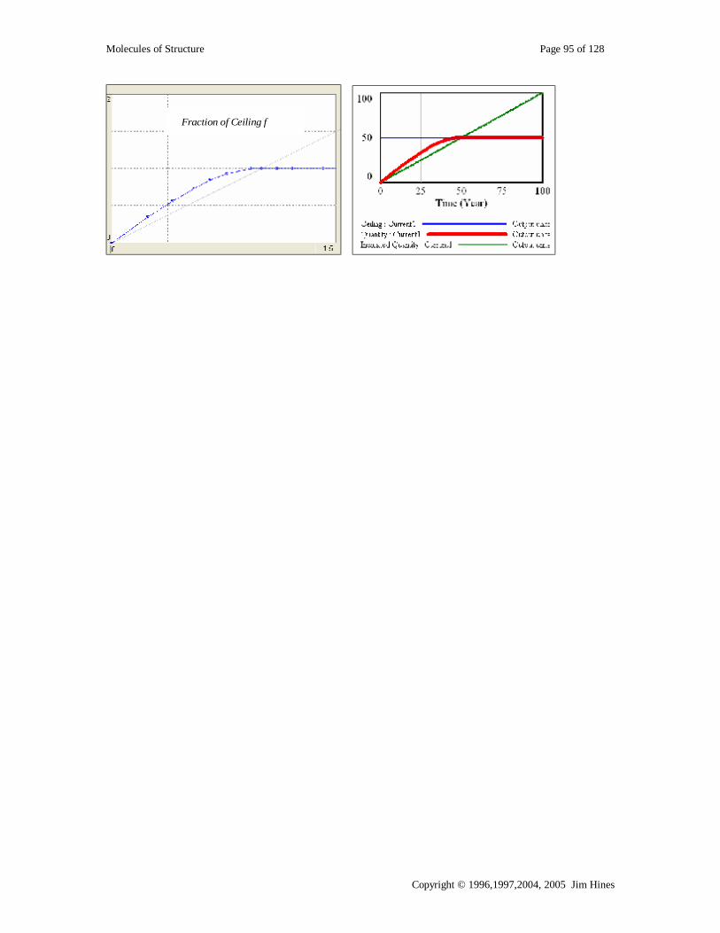
Molecules of Structure Page 95 of 128
Copyright © 1996,1997,2004, 2005 Jim Hines
Fraction of Ceiling f

Molecules of Structure Page 96 of 128
Copyright © 1996,1997,2004, 2005 Jim Hines
Capacity Utilization Immediate parents: Ceiling Ultimate parents: Dmnl input to function, Proportional split Used by: None
Problem solved: How to determine production when desired production can exceed capacity.
Equations:
Production = Capacity * Utilization Units: Widgets/Week Capacity = ___ Units: Widgets/Week Utilization = Utilization f ( IndicatedUtilization ) Units: fraction ndicatedUtilization = DesiredProduction / Capacity Units: fraction DesiredProduction = ___ Units: Widgets/Week Utilization f ( ) = [User defined function] Units: dmnl Description: Production is determined by the fraction of capacity actually used (i.e. utilization). As desired production increases, utilization increases, but only until the capacity is maxed out. Often, modelers allow utilization to go above 1, representing a situation where output can exceed “rated” capacity through skipping routine maintenance shut downs, eliminating the use of the facilities for testing, or other measures.
Behavior: no stocks, so no dynamics.
Classic examples: Common
Caveats: If the function does not go through the point (1,1) calculating an analytical equilibrium for the model will be a bit more difficult.
Technical notes: none
DesiredProduction
Capacity
ProductionIndicatedUtilization
Utilization<Utilization
f>

Molecules of Structure Page 97 of 128
Copyright © 1996,1997,2004, 2005 Jim Hines
Floor Also known as SoftMax Immediate parents: Univariate anchoring and adjustment Ultimate parents: Dmnl input to function Used by: None
Problem solved: How to represent a variable that cannot decline lower than a certain point.
Equations:
Quantity = Floor * Floor Multiple Units: Output units Floor = ___ Units: Output units Floor Multiple = Floor Multiple f ( Indicated Floor Multiple ) Units: dmnl Floor Multiple f = see technical notes Units: dmnl Indicated Floor Multiple = Indicated Quantity / Floor Units: dimensionless Indicated Quantity = ___ Units: Output units
Description: This formulation is a continuous version of the discrete MAX function. Unlike the MAX function -- where the output quantity is either the indicated quantity or the ceiling, whichever is greater – in this formulation the output does not suddenly equal the floor, rather there is a gradual approach. Depending on how the Floor Multiple f is parameterized, the floor can be reached either before or after the IndicatedQuantity equals the floor. (see technical notes). It is also possible to let the Quantity fall below the floor.
Behavior: No levels so no endogenous behavior.
Classic examples: This formulation formed is much rarer than its counterpart, the Ceiling.
Caveats: Make sure that the table function rises high enough to cover the possible range of the indicated floor multiple.
Technical notes: The following shows the behavior of the Quantity for various shapes of the function Floor Multiple f. The shape of the middle function yields behavior that is identical to the discrete MAX function.
IndicatedQuantity
Floor
QuantityIndicatedFloor
Multiple
FloorMultiple
<FloorMultiple f>

Molecules of Structure Page 98 of 128
Copyright © 1996,1997,2004, 2005 Jim Hines

Molecules of Structure Page 99 of 128
Copyright © 1996,1997,2004, 2005 Jim Hines
Level Protected by Flow
Immediate parents: Ceiling, Go to zero Ultimate parents: Dmnl input to function, Go to zero, Proportional split Used by: BacklogShipping Protected By Flow
Problem solved: How to ensure that a stock does not go negative
Equations:
draining = Maximum outflow * fractionOfMaxOutflow Units: Widgets/Month Maximum outflow = Level to drain / Fastest draining time Units: Widgets/Month Fastest draining time = ___ Units: Month Level to drain = INTEG( - draining , ___) Units: Widgets fractionOfMaxOutflow = Fraction of Max f ( IndicatedFractionOfMax ) Units: dmnl Fraction of Max f = see technical notes Units: dmnl IndicatedFractionOfMax = xidz ( Desired draining , Maximum outflow , reallyBigNumber) Units: dmnl reallyBigNumber=10e9 Units: dmnl Desired draining = ___ Units: Widgets/Month
Description: This formulation ensures that the actual outflow from a stock is between the desired outflow and the maximum outflow. This formulation is considered more desirable than an IF-THEN-ELSE statement both because it is less subject to integration error and, even more importantly, because it is appropriate for a stock that represents an aggregation of non-identical items - like a finished goods inventory containing many different models or products.
Level todrain draining
FastestdrainingtimeMaximumoutflow Desired
draining
IndicatedFractionOfMax
fractionOfMaxOutflow
Fraction ofMax f
CurrentLevel to drain
5037.5025.0012.50
0.0014draining
2015.0010.005.002
0.00282.5 5.4 8.4
Time (Month)
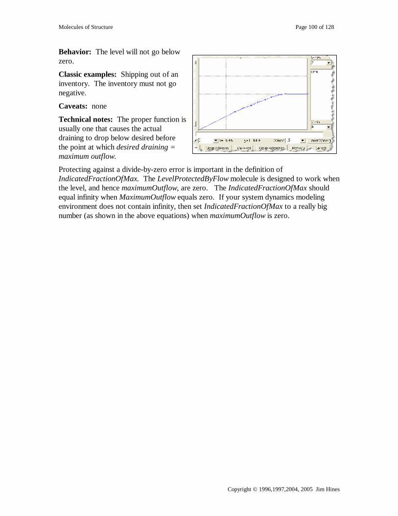
Molecules of Structure Page 100 of 128
Copyright © 1996,1997,2004, 2005 Jim Hines
Behavior: The level will not go below zero.
Classic examples: Shipping out of an inventory. The inventory must not go negative.
Caveats: none
Technical notes: The proper function is usually one that causes the actual draining to drop below desired before the point at which desired draining = maximum outflow.
Protecting against a divide-by-zero error is important in the definition of IndicatedFractionOfMax. The LevelProtectedByFlow molecule is designed to work when the level, and hence maximumOutflow, are zero. The IndicatedFractionOfMax should equal infinity when MaximumOutflow equals zero. If your system dynamics modeling environment does not contain infinity, then set IndicatedFractionOfMax to a really big number (as shown in the above equations) when maximumOutflow is zero.
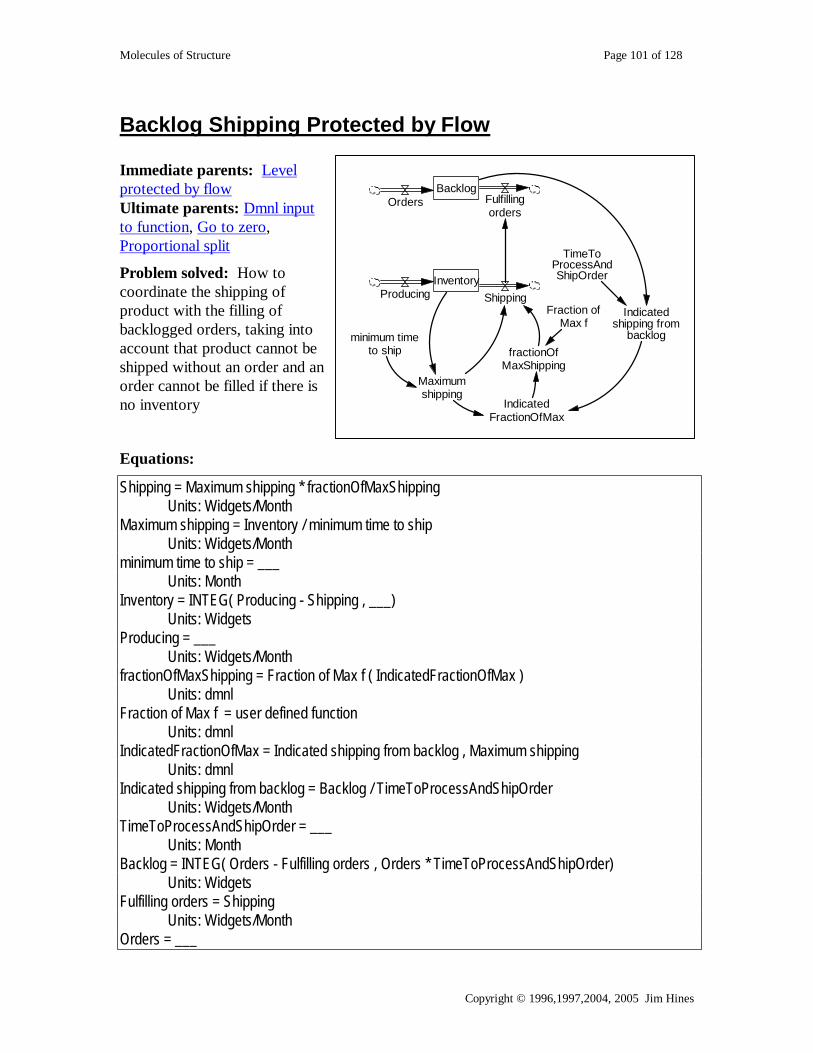
Molecules of Structure Page 101 of 128
Copyright © 1996,1997,2004, 2005 Jim Hines
Backlog Shipping Protected by Flow Immediate parents: Level protected by flow Ultimate parents: Dmnl input to function, Go to zero, Proportional split
Problem solved: How to coordinate the shipping of product with the filling of backlogged orders, taking into account that product cannot be shipped without an order and an order cannot be filled if there is no inventory
Equations:
Shipping = Maximum shipping * fractionOfMaxShipping Units: Widgets/Month Maximum shipping = Inventory / minimum time to ship Units: Widgets/Month minimum time to ship = ___ Units: Month Inventory = INTEG( Producing - Shipping , ___) Units: Widgets Producing = ___ Units: Widgets/Month fractionOfMaxShipping = Fraction of Max f ( IndicatedFractionOfMax ) Units: dmnl Fraction of Max f = user defined function Units: dmnl IndicatedFractionOfMax = Indicated shipping from backlog , Maximum shipping Units: dmnl Indicated shipping from backlog = Backlog / TimeToProcessAndShipOrder Units: Widgets/Month TimeToProcessAndShipOrder = ___ Units: Month Backlog = INTEG( Orders - Fulfilling orders , Orders * TimeToProcessAndShipOrder) Units: Widgets Fulfilling orders = Shipping Units: Widgets/Month Orders = ___
Inventory
Backlog
Producing
Orders Fulfillingorders
ShippingIndicated
shipping frombacklog
TimeToProcessAndShipOrder
minimum timeto ship
Maximumshipping
IndicatedFractionOfMax
fractionOfMaxShipping
Fraction ofMax f
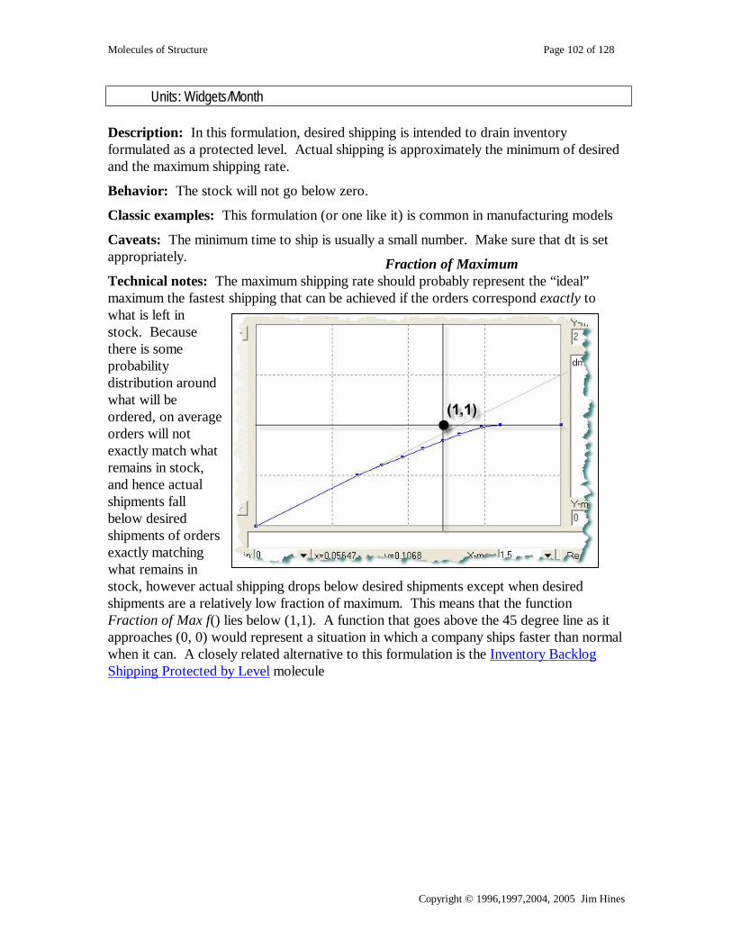
Molecules of Structure Page 102 of 128
Copyright © 1996,1997,2004, 2005 Jim Hines
Units: Widgets/Month Description: In this formulation, desired shipping is intended to drain inventory formulated as a protected level. Actual shipping is approximately the minimum of desired and the maximum shipping rate.
Behavior: The stock will not go below zero.
Classic examples: This formulation (or one like it) is common in manufacturing models
Caveats: The minimum time to ship is usually a small number. Make sure that dt is set appropriately.
Technical notes: The maximum shipping rate should probably represent the “ideal” maximum the fastest shipping that can be achieved if the orders correspond exactly to what is left in stock. Because there is some probability distribution around what will be ordered, on average orders will not exactly match what remains in stock, and hence actual shipments fall below desired shipments of orders exactly matching what remains in stock, however actual shipping drops below desired shipments except when desired shipments are a relatively low fraction of maximum. This means that the function Fraction of Max f() lies below (1,1). A function that goes above the 45 degree line as it approaches (0, 0) would represent a situation in which a company ships faster than normal when it can. A closely related alternative to this formulation is the Inventory Backlog Shipping Protected by Level molecule
Fraction of Maximum

Molecules of Structure Page 103 of 128
Copyright © 1996,1997,2004, 2005 Jim Hines
Backlog Shipping Protected By Level Immediate parents: Go to zero, Level protected by level Ultimate parents: Go to zero, Dmnl input to function Used by: None
Problem solved: How to coordinate the shipping of product with the filling of backlogged orders, taking into account that product cannot be shipped without an order and an order cannot be filled if there is no inventory Equations:
Backlog = INTEG( Orders - Fulfilling orders , Orders * Desired shipping time) Units: Widgets Desired inventory = ___ Units: Widgets Desired shipping = Backlog / Desired shipping time Units: Widgets/Month Desired shipping time = ___ Units: Month Fulfilling orders = Shipping Units: Widgets/Month Inventory = INTEG( Producing - Shipping , Desired inventory ) Units: Widgets Inventory effect on shipping = Inventory effect on shipping f ( Relative inventory) Units: dmnl Inventory effect on shipping f = user defined function Units: dmnl Orders = ___ Units: Widgets/Month Producing = ___ Units: Widgets/Month Relative inventory = Inventory / Desired inventory Units: dmnl Shipping = Desired shipping * Inventory effect on shipping Units: Widgets/Month
Inventory
Backlog
Producing
Orders Fulfillingorders
Shipping
Desiredshipping
Desiredshipping time
Inventory effecton shipping
Inventory effecton shipping f
Desiredinventory
Relativeinventory

Molecules of Structure Page 104 of 128
Copyright © 1996,1997,2004, 2005 Jim Hines
Description: In this formulation, desired shipping is intended to drain inventory formulated as a protected level. Actual shipping however also obeys the physical law that we can’t ship what we don’t have. The backlog is depleted by actual shipping.
Behavior: Obvious
Classic examples: This formulation is common in manufacturing models
Caveats: None
Technical notes: The Inventory Effect on Shipping represents the impact of stockouts as the inventory gets lower and lower. A closely related alternative to this formulation is the Inventory Backlog and Shipping Protected by Flow molecule.

Molecules of Structure Page 105 of 128
Copyright © 1996,1997,2004, 2005 Jim Hines
Weighted Average Also known as Soft If Then Parents: None
Used by: Activity split
Problem solved: How to represent a blend of two “pure” choices.
Equations:
Resulting quantity = WeightOnA * OptionA + (1-WeightOnA) * OptionB Units: people OptionA = ___ Units: people Option B = ___ Units: people WeightOnA = weight on A f(RelativeX) Units: dmnl weightOnA f = user defined function Units: dmnl RelativeX = X / totalXandY Units: fraction totalXAndY= X + Y Units: widgets/week X = ___ Units: widgets/week Y = ___ Units: widgets/week Description: As X increases relative to Y, the blend favors A relative to B.
Behavior: No internal dynamics because no levels.
Classic examples:
Caveats: None
Technical notes: The structure is a generalization of the common if-then logic in computer programming. For example the statement IF X < Y THEN A ELSE B
is represented by a one weighting function. In particular, the “weight on A function” for this example would be
1 when X/Y<1 f(X/Y) = 0 when X/Y ≥ 1
1
0
1
{
Option A Option B
RelativeX
Weight on A
Resultingquantity
XY
weight on A f
totalXAndY

Molecules of Structure Page 106 of 128
Copyright © 1996,1997,2004, 2005 Jim Hines
Diffusion Immediate parents: Proportional split, Conversion Ultimate parents: Proportional split, Bathtub
Used by: None
Problem solved: How to represent growth by word of mouth
Equations:
customers = INTEG(converting, ___) Units: people converting = wom Conversions Units: people/Year wom Conversions = contacts of noncust with cust*fruitfulness Units: people/Year fruitfulness = ___ Units: people/contact contacts of noncust with cust = contacts with customers*PotCust concentration Units: contacts/Year contacts with customers = customers*sociability Units: contacts/Year sociability = ___ Units: contacts/person/Year PotCust concentration = potential customers/total market Units: dmnl total market = customers+potential customers Units: people potential customers = INTEG(-converting, ___) Units: people
Description: Non Customers become customers through a process that involves customers having contacts with people, some fraction of which are non-customers. Some proportion of contacts that customers have with non-customers results in conversion of non-customers to customers.
womConversions
customerspotentialcustomers
contacts ofnoncust with cust
converting
fruitfulness
contacts withcustomers
PotCustconcentration
total market
sociability

Molecules of Structure Page 107 of 128
Copyright © 1996,1997,2004, 2005 Jim Hines
Behavior: Produces S-shaped growth in customers.
Classic examples: This is the structure that underlies B&B Enterprises.
Caveats: If customers are initialized to zero this structure will not move because there will be no customers to have contacts.
Technical notes: This structure produces logistic growth. The Bass diffusion model includes an addition flow, formulated as a decay from potential customers into customers. This additional flow is often interpreted as being an effect of advertising. With this additional flow, the initial value of customers can be set to zero.
BEHAVIORcustomers
100 M75.00 M50.00 M25.00 M
1,000converting
31.24 M23.43 M15.62 M7.812 M
166.490 10 20
Time (Year)

Molecules of Structure Page 108 of 128
Copyright © 1996,1997,2004, 2005 Jim Hines
Action From Resource Immediate parents: None Ultimate parents: None Used by: Producing, Resource from flow, Ability from flow, Financial flow from resource
Problem solved: How to create an action (a flow) from a resource or aggregate of resources.
Equations:
flow = resources * resourceAbilityToCreateFlow Units: gallons/Month resourceAbilityToCreateFlow = ___ Units: gallons/(Month*resource) resources = ___ Units: resources
Description: The action (flow) is created by multiplying a resource by its ability to create an action (i.e. its productivity). Often the activity will be conceptualized as a flow, as shown in the structure above.
Behavior: No stocks, so no loops so no behavior.
Classic examples: Producing, Financial flow from resource
Caveats: None
Technical notes: This is one of three general ways to create an action. The other two are Close gap and Go to zero
resources resourceAbilityToCreateFlow
flow
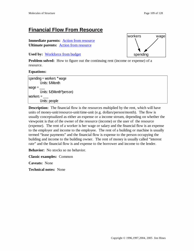
Molecules of Structure Page 109 of 128
Copyright © 1996,1997,2004, 2005 Jim Hines
Financial Flow From Resource Immediate parents: Action from resource Ultimate parents: Action from resource Used by: Workforce from budget
Problem solved: How to figure out the continuing rent (income or expense) of a resource.
Equations:
spending = workers * wage Units: $/Month wage = ___ Units: $/(Month*person) workers = ___ Units: people
Description: The financial flow is the resources multiplied by the rent, which will have units of money-unit/resource-unit/time-unit (e.g. dollars/person/month). The flow is usually conceptualized as either an expense or a income stream, depending on whether the viewpoint is that of the owner of the resource (income) or the user of the resource (expense). The rent of a worker is her wage or salary and the financial flow is an expense to the employer and income to the employee. The rent of a building or machine is usually termed “lease payments” and the financial flow is expense to the person occupying the building and income to the building owner. The rent of money is usually called “interest rate” and the financial flow is and expense to the borrower and income to the lender.
Behavior: No stocks so no behavior.
Classic examples: Common
Caveats: None
Technical notes: None
workers wage
spending

Molecules of Structure Page 110 of 128
Copyright © 1996,1997,2004, 2005 Jim Hines
Resources From Action Immediate parents: Action from resource Ultimate parents: Action from resource Used by: Workforce from budget
Problem solved: How to determine the resources we have (or need) based on the (desired) action (or flow) and the resources’ ability to create the action (i.e. the resources’ productivity)
Equations:
esources = DesiredFlow / resourceAbilityToCreateFlow Units: resources resourcesDesiredFlow = -___ Units: gallons/Month resourceAbilityToCreateFlow = ___ Units: gallons/(Month*resource) r Description: Given the action (flow), dividing by the resource’s creative ability (productivity) yields the necessary resources.
Behavior: No stocks so no behavior
Classic examples: Workorce from budget in Jay Forrester’s Market Growth as Influenced by Capital Investment.
Caveats: None
Technical notes: None
resources
resourceAbilityToCreateFlow
DesiredFlow
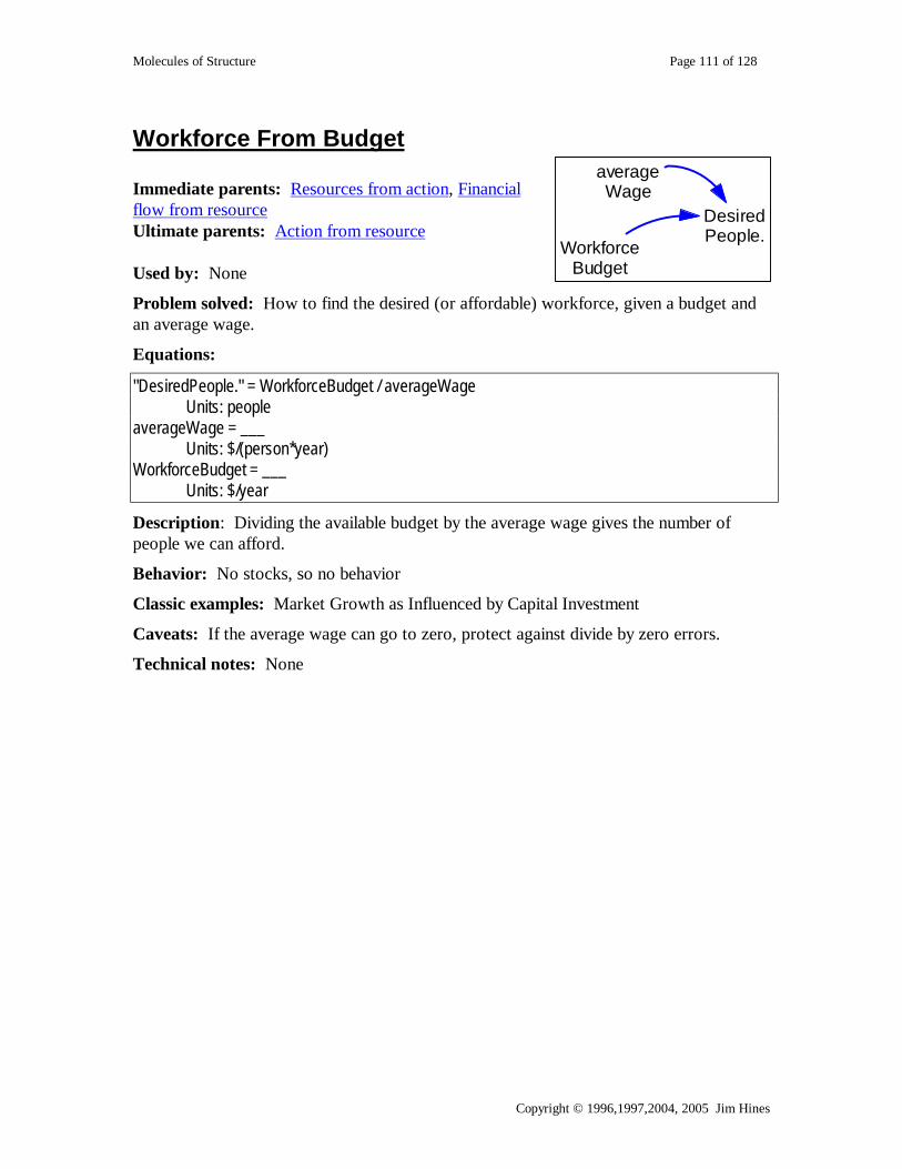
Molecules of Structure Page 111 of 128
Copyright © 1996,1997,2004, 2005 Jim Hines
Workforce From Budget Immediate parents: Resources from action, Financial flow from resource Ultimate parents: Action from resource Used by: None
Problem solved: How to find the desired (or affordable) workforce, given a budget and an average wage.
Equations:
"DesiredPeople." = WorkforceBudget / averageWage Units: people
averageWage = ___ Units: $/(person*year) WorkforceBudget = ___
Units: $/year
Description: Dividing the available budget by the average wage gives the number of people we can afford.
Behavior: No stocks, so no behavior
Classic examples: Market Growth as Influenced by Capital Investment
Caveats: If the average wage can go to zero, protect against divide by zero errors.
Technical notes: None
DesiredPeople.
averageWage
WorkforceBudget

Molecules of Structure Page 112 of 128
Copyright © 1996,1997,2004, 2005 Jim Hines
Ability From Action Immediate parents: Action from resource Ultimate parents: Action from resource Used by: Estimated productivity
Problem solved: How to figure out what the creative ability (e.g. productivity) is a resource if we know the activity (or flow) that it causes.
Equations:
Ability = Flow / Resource Units: gallons/(resource*Month) Flow = ___ Units: gallons/Month Resource = ___ Units: resources
Description: The creative ability of a resource is simply the action (or flow) devided by the resource that generates that activity. This molecule is simply a rearrangement of the elements of the action from resource molecule
Behavior: No stocks so no behavior
Classic examples: Sometimes used to figure out productivity in project models (see Estimated productivity).
Caveats: If the resource can go to zero, protect against a of divide-by-zero error.
Technical notes: None.
Resource
Ability
Flow
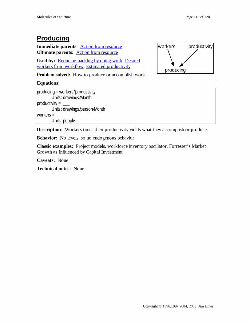
Molecules of Structure Page 113 of 128
Copyright © 1996,1997,2004, 2005 Jim Hines
Producing Immediate parents: Action from resource Ultimate parents: Action from resource
Used by: Reducing backlog by doing work, Desired workers from workflow, Estimated productivity
Problem solved: How to produce or accomplish work
Equations:
producing = workers*productivity Units: drawings/Month productivity = ___ Units: drawings/person/Month workers = ___ Units: people
Description: Workers times their productivity yields what they accomplish or produce.
Behavior: No levels, so no endogenous behavior
Classic examples: Project models, workforce inventory oscillator, Forrester’s Market Growth as Influenced by Capital Investment
Caveats: None
Technical notes: None
workers productivity
producing

Molecules of Structure Page 114 of 128
Copyright © 1996,1997,2004, 2005 Jim Hines
Estimated Productivity Immediate parents: Ability from action, Producing Ultimate parents: Action from resource Used by: None
Problem solved: Estimating productivity
Equations:
EstimatedPDY = WorkBeingAccomplished / Workforce Units: widgets/(person*Month) WorkBeingAccomplished = ___ Units: widgets/Month Workforce = ___ Units: people
Description: Given a flow of work and the number of workers doing it, the implied productivity has to be the flow divided the number of workers.
Behavior: No stocks, so no behavior.
Classic examples: None
Caveats: None
Technical notes: Work being accomplished wouldn’t actually be known by real world managers if it is an actual flow. In this case the modeler may wish to either use a knowable estimate of Work being accomplished (e.g. a smooth of it) or use the estimated PDY from this formulation as an input into a formulation (e.g. a smooth) for perceived productivity.
Workforce
EstimatedPDY
WorkBeingAccomplished

Molecules of Structure Page 115 of 128
Copyright © 1996,1997,2004, 2005 Jim Hines
Desired Workforce From Workflow Immediate parents: Resource from action, Producing Used by: Overtime
Problem solved: How to determine the number of workers we need
Equations:
DesiredPeople = DesiredAccomplishingRate / productivity Units: people productivity = ___ Units: SquareFeet/person/Week DesiredAccomplishingRate = ___
Description: The key here is the rate at which we need to accomplish work in order to finish on time. Once we know this, we can figure out how many people it takes to produce such a work flow.
Behavior: No levels so no endogenous behavior.
Classic examples: Most project models make use of a formulation like this one.
Caveats: None
Technical notes: This formulation uses the same understanding as that used in the Producing molecule. Outputs and inputs, though, are different. Here we know the (desired) production rate and we calculate the (desired) workforce. In the Producing molecule we know the workforce and calculate the production rate. In this formulation, we could use a perceived productivity.
DesiredPeople
productivity
DesiredAccomplishing
Rate
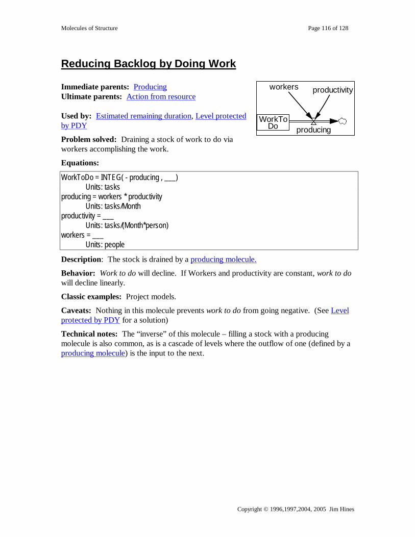
Molecules of Structure Page 116 of 128
Copyright © 1996,1997,2004, 2005 Jim Hines
Reducing Backlog by Doing Work Immediate parents: Producing Ultimate parents: Action from resource Used by: Estimated remaining duration, Level protected by PDY
Problem solved: Draining a stock of work to do via workers accomplishing the work.
Equations:
WorkToDo = INTEG( - producing , ___) Units: tasks producing = workers * productivity Units: tasks/Month productivity = ___ Units: tasks/(Month*person) workers = ___ Units: people
Description: The stock is drained by a producing molecule.
Behavior: Work to do will decline. If Workers and productivity are constant, work to do will decline linearly.
Classic examples: Project models.
Caveats: Nothing in this molecule prevents work to do from going negative. (See Level protected by PDY for a solution)
Technical notes: The “inverse” of this molecule – filling a stock with a producing molecule is also common, as is a cascade of levels where the outflow of one (defined by a producing molecule) is the input to the next.
workers productivity
WorkToDo producing

Molecules of Structure Page 117 of 128
Copyright © 1996,1997,2004, 2005 Jim Hines
Level Protected by PDY
workers
productivity
RemainingWork producing
RequiredWorkForFull
Productivity
RelativeRemainingWork
EffectOfRemainingWorkOnPDY
normalPDY
EffectOfRemainingWork
OnPDY f
workers.
productivity.
RemainingWork. producing.
RequiredWorkForFullProductivity.
requiredWorkToKeepAWorker
Occuppied.
RelativeRemainingWork.
EffectOfRemainingWorkOnPDY.
normalPDY.
EffectOfRemainingWorkOnPDY f.
Immediate parents: Reducing backlog by doing work, Univariate anchoring and adjustment Ultimate parents: Action From Resource, Dmnl input to function Used by: None
Problem solved: How to prevent the level of remaining work going below zero when workers are producing from a backlog.
Equations:
RemainingWork = INTEG( - producing , RequiredWorkForFullProductivity ) Units: tasks producing = workers * productivity Units: tasks/Month workers = ___ Units: people productivity = normalPDY * EffectOfRemainingWorkOnPDY Units: tasks/(person*Month) normalPDY = 5 Units: tasks/(person*Month) EffectOfRemainingWorkOnPDY = EffectOfRemainingWorkOnPDY f ( RelativeRemainingWork ) Units: dmnl EffectOfRemainingWorkOnPDY f = user defined function Units: dmnl

Molecules of Structure Page 118 of 128
Copyright © 1996,1997,2004, 2005 Jim Hines
RelativeRemainingWork = RemainingWork / RequiredWorkForFullProductivity Units: fraction RequiredWorkForFullProductivity = ___ Units: tasks Additional equations for second version "RequiredWorkForFullProductivity." = "workers." * "requiredWorkToKeepAWorkerOccuppied." Units: tasks "requiredWorkToKeepAWorkerOccuppied." = ___ Units: tasks/person
Description: This molecule solves the problem of the stock in the reducing backlog by doing work molecule going negative as workers continue to drain the stock after it hits zero. The solution is to recognize that productivity must become zero when there are no longer any tasks to do. As the level of tasks falls below an amount of tasks required for full productivity, the resource’s productivity falls. This could be because there is a time consuming step (e.g. having to bake clay pots in a kiln for two days) and to reach full productivity a worker needs enough other tasks to occupy him during the time that other tasks are in the time-consuming phase. In a formulation where the single workforce is an aggregate of a number of different skills, the reduction of productivity could be caused by workers having to take on tasks for which they are not in their “specialty” and hence on which they are less productive.
The second version of the molecule includes a formulation for the number of tasks required for full productivity. This formulation says that each worker needs (on average) a certain number of tasks in the backlog in order to work at full productivity.
Behavior: The stock will not fall below zero.
Classic examples: The balancing R&D chain model
Caveats: None
Technical notes: None
RemainingWork15
11.25
7.502
3.754
0.00560 0.20 0.40 0.60 0.80 1 1.20 1.40 1.60 1.80 2
Time (Month)

Molecules of Structure Page 119 of 128
Copyright © 1996,1997,2004, 2005 Jim Hines
Estimated remaining duration Immediate parents: Reducing backlog by doing work Ultimate parents: Action from resource
Used by: Estimated completion date
Problem solved: How to estimate the remaining time to completion of an amount of work to do. How to estimate the average time to complete a task in a stock of work to do (see technical note).
Equations:
DurationTillComplete = WorkToDo / AnticipatedRateOfAccomplishingWork Units: week WorkToDo = ___ Units: square feet AnticipatedRateOfAccomplishingWork = ___ Units: square feet / week
Description: The estimated duration to completion is simply the amount of work left divided by the rate at which we can do the work.
Behavior: No levels, so no endogenous behavior.
Classic examples: Used in project models
Caveats: If people or productivity can be zero, you will need to protect against a divide by zero error in the equation for durationTillComplete.
Technical notes: This formulation is related to the residence time molecule. Consequently, the variable durationUntilComplete can also be interpreted as the estimated average time to complete an individual task in the stock of work to do. Under this interpretation the variable’s name should be changed to something more appropriate (e.g. estimatedTaskResidenceTime).
WorkToDo
DurationTillComplete
AnticipatedRateOfAccomplishing
Work
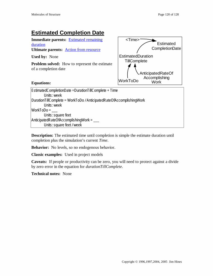
Molecules of Structure Page 120 of 128
Copyright © 1996,1997,2004, 2005 Jim Hines
Estimated Completion Date Immediate parents: Estimated remaining duration Ultimate parents: Action from resource
Used by: None
Problem solved: How to represent the estimate of a completion date
Equations:
EstimatedCompletionDate =DurationTillComplete + Time Units: week DurationTillComplete = WorkToDo / AnticipatedRateOfAccomplishingWork Units: week WorkToDo = ___ Units: square feet AnticipatedRateOfAccomplishingWork = ___ Units: square feet / week Description: The estimated time until completion is simple the estimate duration until completion plus the simulation’s current Time.
Behavior: No levels, so no endogenous behavior.
Classic examples: Used in project models
Caveats: If people or productivity can be zero, you will need to protect against a divide by zero error in the equation for durationTillComplete.
Technical notes: None
EstimatedCompletionDate
WorkToDo
EstimatedDurationTillComplete
<Time>
AnticipatedRateOfAccomplishing
Work

Molecules of Structure Page 121 of 128
Copyright © 1996,1997,2004, 2005 Jim Hines
Overtime Immediate parents: Workforce, Univariate anchoring and adjustment, Desired workers from workflow Ultimate parents: Smooth (first order), Flow from resource, Dmnl input to function
Used by: none
Problem solved: How to calculate the required amount of overtime.
Equations:
Overtime = Overtime f ( IndicatedOvertime ) Units: Fraction Overtime f = user defined function Units: Fraction IndicatedOvertime = DesiredPeople / Workers Units: Fraction Workers = 10 Units: people DesiredPeople = DesiredAccomplishingRate / productivity Units: people DesiredAccomplishingRate = ___ Units: tasks/week productivity = ___ Units: tasks/(week*person) Description: Overtime might be measured as a fraction of a normal day. If possible overtime would simply be the number of workers we wished we had divided by the number of workers we actually have. In practice, of course, the amount of overtime is limited by the number of hours in a day, by management policy, and by what workers are willing to do. The overtime function represents this practical limitation.
Behavior: No levels so no endogenous behavior.
Classic examples: Formulation like this are used in many project models.
Caveats: If the workforce can be zero, the modeler needs to protect against a divide by zero error in the calculation of IndicatedOvertime.
Technical notes: DesiredPeople here means “people needed to get the work done”. Any formulation that yields such a definition of desired people is fine. Although we use the desired workers from workflow molecule, other formulation are possible.
OvertimeIndicatedOvertime
Workers
Overtime fDesiredPeople
productivity
DesiredAccomplishingRate

Molecules of Structure Page 122 of 128
Copyright © 1996,1997,2004, 2005 Jim Hines
Building Inventory by Doing Work Immediate parents: Producing Ultimate parents: Action from resource Used by: Population growth, Doing work cascade
Problem solved: How to create an inventory inflow from people working.
Equations:
Inventory = INTEG( producing , ___ Units: widgets producing = workers * productivity Units: widgets/Month productivity = ___ Units: widgets/(Month*person) workers = ___ Units: people Description: The inflow to the stock is a producing molecule.
Behavior: If workers and productivity are constant, the stock will rise linearly.
Classic examples: Workforce Inventory Oscillator
Caveats: None
Technical notes: None
workers productivity
producingInventory

Molecules of Structure Page 123 of 128
Copyright © 1996,1997,2004, 2005 Jim Hines
Population Growth Immediate parents: Building inventory by doing work Ultimate parents: Action from resource Used by: None
Problem solved:
Equations:
Population = INTEG( birthing , ___ Units: people birthing = Population * fertility Units: people/Month fetility = ___ Units: people/(Month*person)
Description: The inflow to population is the population multiplied by the average fertility of the population.
Behavior: Exponential growth (if fertility is a constant).
Classic examples: Common
Caveats: With a large enough growth rate or a long enough simulation length, this formulation can produce a population size that exceeds the largest number the computer can represent. In this case, the machine will throw a floating point overflow error and the simulation will stop.
Technical notes: Fertility is the productivity of the population in producing babies. This is simply a Building Inventory by Doing Work molecule where the “inventory” is the workforce itself.
fertility
birthingPopulation
CurrentPopulation54.3240.9927.6614.33
1birthing2.1731.6391.106
0.57320.04
0 50 100Time (Month)
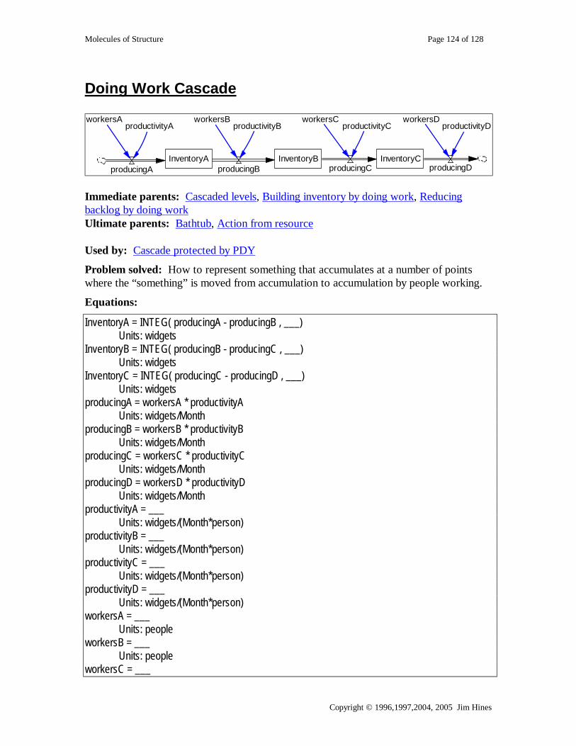
Molecules of Structure Page 124 of 128
Copyright © 1996,1997,2004, 2005 Jim Hines
Doing Work Cascade
workersBproductivityB
producingBInventoryB
workersCproductivityC
producingCInventoryC
workersAproductivityA
producingAInventoryA
producingD
productivityDworkersD
Immediate parents: Cascaded levels, Building inventory by doing work, Reducing backlog by doing work Ultimate parents: Bathtub, Action from resource Used by: Cascade protected by PDY
Problem solved: How to represent something that accumulates at a number of points where the “something” is moved from accumulation to accumulation by people working.
Equations:
InventoryA = INTEG( producingA - producingB , ___) Units: widgets InventoryB = INTEG( producingB - producingC , ___) Units: widgets InventoryC = INTEG( producingC - producingD , ___) Units: widgets producingA = workersA * productivityA Units: widgets/Month producingB = workersB * productivityB Units: widgets/Month producingC = workersC * productivityC Units: widgets/Month producingD = workersD * productivityD Units: widgets/Month productivityA = ___ Units: widgets/(Month*person) productivityB = ___ Units: widgets/(Month*person) productivityC = ___ Units: widgets/(Month*person) productivityD = ___ Units: widgets/(Month*person) workersA = ___ Units: people workersB = ___ Units: people workersC = ___

Molecules of Structure Page 125 of 128
Copyright © 1996,1997,2004, 2005 Jim Hines
Units: people workersD = ___ Units: people
Description: A cascade of levels in which the flows are all caused by workers working at some productivity and where the outflow from one level is the inflow into the next.
Behavior: If the workers and their productivities are all constant, the stocks will rise or fall linearly.
Classic examples: R&D Chain
Caveats: There’s nothing to prevent any of these levels from going negative. (See Cascade protected by pdy).
Technical notes: None

Molecules of Structure Page 126 of 128
Copyright © 1996,1997,2004, 2005 Jim Hines
Cascade Protected By PDY
workersB
producingBInventoryC
workersC
producingCInventoryD
workersA
productivityA
producingAInventoryB producingD
workersD
productivityB
RequiredWorkForFullProductivityB
RelativeRemaining
WorkB
EffectOfRemainingWork
OnPDYB normalPDYB
EffectOfRemainingWork
OnPDYB f
productivityC
RequiredWorkForFullProductivityC
RelativeRemaining
WorkC
EffectOfRemainingWork
OnPDYC
normalPDYC
EffectOfRemainingWorkOnPDYC f
productivityD
RequiredWorkForFull
ProductivityD
RelativeRemaining
WorkD
EffectOfRemainingWork
OnPDYD
normalPDYD
EffectOfRemainingWork
OnPDYD f Immediate parents: Level protected by PDY, Doing work cascade Ultimate parents: Close gap, Action from resource, Dmnl input to function, Bathtub Used by: None
Problem solved: How to prevent workers from drawing down cascaded levels below zero.
Equations:
InventoryB = INTEG( producingA - producingB , RequiredWorkForFullProductivityB ) Units: widgets InventoryC = INTEG( producingB - producingC , RequiredWorkForFullProductivityC ) Units: widgets InventoryD = INTEG( producingC - producingD , RequiredWorkForFullProductivityD ) Units: widgets producingA = workersA * productivityA Units: widgets/Month producingB = workersB * productivityB Units: widgets/Month producingC = workersC * productivityC Units: widgets/Month producingD = workersD * productivityD Units: widgets/Month workersA = 5 Units: people workersB = 5 Units: people workersC = 5

Molecules of Structure Page 127 of 128
Copyright © 1996,1997,2004, 2005 Jim Hines
Units: people workersD = 12 Units: people productivityA = 5 Units: widgets/(Month*person) productivityB = normalPDYB * EffectOfRemainingWorkOnPDYB Units: widgets/(Month*person) productivityC = normalPDYC * EffectOfRemainingWorkOnPDYC Units: widgets/(Month*person) productivityD = normalPDYD * EffectOfRemainingWorkOnPDYD Units: widgets/(Month*person) normalPDYB = 5 Units: widgets/(Month*person) normalPDYC = 5 Units: widgets/(Month*person) normalPDYD = 5 Units: widgets/(Month*person) EffectOfRemainingWorkOnPDYB= EffectOfRemainingWorkOnPDYB f( RelativeRemainingWorkB ) Units: dmnl EffectOfRemainingWorkOnPDYB f = user defined function Units: dmnl EffectOfRemainingWorkOnPDYC= EffectOfRemainingWorkOnPDYC f( RelativeRemainingWorkC ) Units: dmnl EffectOfRemainingWorkOnPDYC f = user defined function Units: dmnl EffectOfRemainingWorkOnPDYD= EffectOfRemainingWorkOnPDYD f (RelativeRemainingWorkD ) Units: dmnl EffectOfRemainingWorkOnPDYD f = user defined function Units: dmnl RelativeRemainingWorkB = InventoryB / RequiredWorkForFullProductivityB Units: fraction RelativeRemainingWorkC = InventoryC / RequiredWorkForFullProductivityC Units: fraction RelativeRemainingWorkD = InventoryD / RequiredWorkForFullProductivityD Units: fraction RequiredWorkForFullProductivityB = 15 Units: widgets RequiredWorkForFullProductivityC = 15 Units: widgets RequiredWorkForFullProductivityD = 15 Units: widgets
Description: People working (at some productivity) cause material to flow through a chain of accumulations. The productivity of the people working on any one flow is a function of the amount of material in stock that is being drained (i.e. a function of the amount of material in the source).

Molecules of Structure Page 128 of 128
Copyright © 1996,1997,2004, 2005 Jim Hines
Behavior: The levels will not go negative.
Classic examples: R&D Balance Chain
Caveats: None
Technical notes: None