AD-A1IM 114 ON THE DISSIPATIVE RESPONSE DU TO DISCONTINUOUS v/1STRAINS IN MRS OF UNSTA.. (U) CALIFORNIA INST OF TECHPASADENA DIV OF ENGINEERING AND APPLI.

UNLFSSFID BERRTN E A.SEP 87 TR-1 F/G 20/11 N

mohEmhhmhhhhhE

I lfflll~lf.fllff

as~ 12.2*--r-

Di-

Ii __

~ 1.1

MICROCOPY RESOLUTION TEST CHARTNATIONAL BUREAU OFr STANDARDS-1963-A

I

I .. -

4|

D CFILE COY..

Technical Report No.

Co ON THE DISSIPATIVE RESPONSE DUE TO DISCONTI.NUOUS

STRAINS IN BARS OF UNSTABLE ELASTIC HATERIAL

.1- E C

& 0 &C 00

........... .... 110 1p 4 .M!

-, . ...... *. A A ALIFORNIA.I- F--.'

- .: AP~rov.I1 ki public rolocwel .'4

87 1127 217.-

4.L

Office of Naval Research

Contract NOO0l4-87-K.0117 ?F T

Technical Report No. I Li)

ON THE DISSIPATIVE RESPONSE DUE TO DISCONTINUOUS

STRAINS IN BARS OF UNSTABLE ELASTIC MATERIAL

by

Rohazi Abyra * and Jamos*K. Knowles

*Departmenxt of Mechanical EngineeringMassachusetts Institute of Technology

Cambridge, Massachusetts 02139

**Division of Engineering and Applied ScienceCalifornia Institute of Technology

Pasadena, California 91125

September, 1987

rAj),Yirr--d fo. ;Diwfthbutj .A Uni . ,

ABSTRACTVSome elastic materials are capable of sustaining finite

equilibrium deformations with discontinuous strains. Boundary-

value problems for such "unstable" elastic materials often

possess an infinity of solutions. suggesting that the theory

suffers from a constitutive deficiency. In the setting of the

one-dimensional theory of bars in tension, the present paper

ezplores the consequences of supplementing the theory with

further constitutive information. This additional information

pertains to the surface of strain discontinuity and consists of a

"kinetic relation" and a criterion for the *initiation" of such a

surface. We show that the quasi-static response of the bar to a

prescribed force history is then fully determined. In

particular, we observe how unstable elastic meterials can be used

to model macroscopic behavior similar to that associated with

viscoplasticity.

• -i

__I- - 1* .... / ... ....

6a.m I 9M k X 41 I?

-- 2--

1. Introduction

Bodies composed of certain types of homogeneous elastic materials can

be finitely deformed to equilibrium states in which displacement gradients,

strains and stresses suffer jump discontinuities across special surfaces.

Elastostatic fields of this kind arise, for example, in continuum mechani-

cal treatments of stress-induced phase transformations in solids [1,2].

When such jumps in displacement gradient occur during quasi-static,

isothermal motions, the balance between the rate of increase of stored

energy and the rate of work of external forces associated with convention-

ally smooth deformations of elastic bodies no longer holds. This balance is

replaced by one which includes an additional effect that may be interpreted

as the rate of work of a fictitious "driving traction" acting on the moving

surface of discontinuity [3]. The driving traction is formally related to

the notion of a "force on a defect" introduced by Eshelby [4] and discussed

by Rice [5].

The altered energetics of finite elastostatic fields involving strain

jumps suggest that such fields might be used to model certain types of dis-

sipative behavior in solids. The circumstances, in fact, are reminiscent in

some respects of those present in the classical theory of flows of ideal

fluids in which shock waves are present. In the latter subject, shocks

account in an idealized way for the neglected dissipative effects of visco-

sity and heat conduction; see p. 322 of (6]. Because of this similarity, we

refer to surfaces bearing jump discontinuities in the displacement gradient

in an elastostatic field as "equilibrium shocks".

Not all elastic materials are capable of sustaining deformations with

equilibrium shocks. Those that do have this capability are sometimes called

unstable materials; they necessarily lead to differential equations of

equilibrium that fail to remain elliptic at all deformations [7]. This in

turn leads to a massive loss of uniqueness of solution for the boundary

value problems of elastostatics, suggesting the need for additional consti-

tutive assumptions that will select from among the many possible equili-

brium states that one which is preferred by the body. One such additional

constitutive postulate asserts that the material is conservative at all of

its particles, including those on shocks, so that the body prefers that

equilibrium state which renders the appropriate energy functional an abso-

* S r I

-- 3--

lute minimum. With this assumption in force, the driving traction acting on

any equilibrium shock necessarily vanishes [8,9], the conventional balance

between work and energy is preserved, and no dissipation takes place. In

this conservative setting, elastostatic fields with shocks have recently

received much analytical attention; see, for example, [1],[2],[9-16].

In two recent papers [17,18], we have discussed an example in order to

illustrate an alternative constitutive postulate. The problem treated in

[17,18] involves a finite, plane deformation of an infinite medium contain-

ing a circular cavity. A uniform circumferential traction is applied to the

cavity wall, and the displacement is required to vanish at infinity. For

the class of incompressible, isotropic elastic materials considered, the

resulting twisting deformation may exhibit a circular equilibrium shock

concentric with the cavity. In quasi-static motions of the body involving

such equilibrium states, the relationship between the applied torque and

the twist at the cavity wall - i.e., the macroscopic response - is in gen-

eral hysteretic. We show in (17,18] that if a certain maximum-dissipation

postulate is used as the supplementary constitutive assumption, the macros-

copic response mimics that associated with rate-independent elastic-plastic

behavior.

Our purpose in the present paper is to discuss supplementary constitu-

tive models for elastic fields capable of sustaining equilibrium shocks in

more generality. The principal new feature introduced here is a "kinetic

relation" analogous to those arising in microstructural models of plastic

behavior formulated in terms of internal variables [5,19,20]. In our cir-

cumstances, this relation takes the form of a constitutive law connecting

the driving traction acting on a moving shock with the shock velocity dur-

ing a quasi-static, isothermal motion. We show that appropriate choices of

the kinetic relation lead to visco-plastic macroscopic response, and we

recover conservative (minimum-energy) response as well as rate-independent

elastic-plastic behavior as special or limiting cases.

When there is an equilibrium shock in the body, the kinetic law governs

its evolution. However a separate criterion -- an initiation or nucleation

criterion -- is required in order to signal the initial appearance of the

shock. This too will be discussed in the following.

* ~ ~%\ ~ I

For simplicity, we work here in the context of a one-dimensional model

for extensional deformations of an elastic bar. Our setting is thus essen-

tially that of Ericksen (10] in his discussion of one-dimensional deforma-

tions with strain-jumps, except that we consider bars whose cross-sectional

area varies with position. The special case of the unifo bar turns out to

be exceptional in certain important respects.

After introducing in the following section the class of elastic materi-

als to be considered, we investigate equilibrium states with a single shock

in Section 3. Sections 4 and 5 are concerned with the energetics of quasi-

static, isothermal motions of the bar and the admissibility of such motions

according to the second law of thermodynamics. We introduce the notion of a

kinetic relation as well as a shock initiation criterion in Section 6, and

in Section 7 present examples to illustrate the possibilities offered by

the theory.

An approach of the type put forward here may have application to the

modeling of the mechanical response of shape-memory alloys [21], to contin-

uum descriptions of the effect of the presence of a "damaged phase" on the

behavior of solids, and to transformation toughening in ceramic composites

[22].

2. Peiinre

Consider a bar composed of a homogeneous elastic material, which in its

reference configuration occupies the interval [0,L]. Let x denote the coor-

dinate of a generic point of the bar in this configuration. If the refer-

ence cross-sectional area of the bar at x is A(x) > 0, it is assumed that

A G C2 [0,L]. We also assume that A(x) increases monotonically with x, so

that

A'(x) > 0, 0 s x S L. (2.1)

We shall show later that the special case of the unifor bar (A'(x) - 0) is

exceptional in certain respects; it is temporarily excluded from consider-

ation.

A deformation of the bar is characterized by an invertible mapping

9 11

-- 5--

y - x + u(x), 0 x L, (2.2)

which subjects the particle at x to a displacement u and carries it to a

new location y. There is no loss of generality in taking the left-hand end

of the bar to be fixed; if 6 denotes the elongation of the bar,

u(L) - 6, u(O) - 0. (2.3)

It will be necessary in the following to consider displacement fields which

are less than classically smooth, and accordingly we allow for the possi-

bility that, although u is continuous on [0,L], there is a number s e [0,L]

such that (i) u is continuously differentiable on [O,s] + [s,L], (ii) u is

twice continuously differentiable on (O,s) + (s,L), and (iii) u' suffers a

finite jump discontinuity across x - s. The strain e at a particle x - s is

defined by

e(x) - u'(x) > -I, 0 < x < L, x 0 s; (2.4)

the first inequality in (2.4) assures the invertibility of the mapping

(2.2).

Let a(x) be the nominal stress field in the bar. Equilibrium in the

absence of body forces requires

o(x)A(x) - F - constant, 0 : x : L; (2.5)

F denotes the force in the bar. Clearly, a E C2 [0,L.

The material is characterized by an elastic potential W whose value

is the strain energy per unit reference volume. We assume that W is defined

on (-l,-) and that it is twice continuously differentiable there. The

stress response function of the bar (e) is given in terms of W by

()- W'(e), -1 < E < ®, (2.6)

so that by (2.5), the stress at x is

- F/A(x), 0 < x < L, x 0 s. (2.7)

If F is given, the force Droblem consists of finding a displacement field

u of the requisite smoothness conforming to (2.7), (2.4), (2.3)2. If 6 is

given, the elongation Droblem requires the determination of a constant F

and a displacement field u satisfying (2.7), (2.4) and (2.3). We shall be

concerned only with the force problem.

From a thermodynamic viewpoint, the present analysis assumes that con-

ditons are isothermal. The elastic potential W coincides with the Helmholtz

free energy of the material at the given temperature, while the associated

Gibbs free energy G expressed in terms of strain is

G(e) - W(e) - P(e)e, -1 < e < . (2.8)

In this paper we restrict attention to materials whose stress response

function a(e) first increases with increasing e, then decreases, and

finally increases again; see Figure 1. Specifically we suppose that there

are positive numbers EM and em such that ''(cM) - a'(em) - 0, ̂ '(e) > 0 for

-1 < f < eM, a'(e) < 0 for eM < e < em, and a'(c) > 0 for em < C

Moreover,

aM 9(0M) > O, am - O(em) > 0, ^(-) a(-l) - --. (2.9)

Note that these materials are of "Baker-Ericksen type" in the sense that

a(e)e > 0 for eO. For our purposes, it is sufficient to consider only

tensile stresses, so we restrict attention henceforth to a > 0.

Although a(e) is not invertible on (-lo), its restrictions to certain

subsets of this interval do have inverses, and these play a major role in

the analysis to follow. Let IE, e2 , e3 be the functions inverse to the

restrictions of a(E) to the respective intervals (-I,eM], [eMEm], and

[em,0); these inverse functions are defined on (--,aM], [am,aM] and [am,-)

respectively. Each function f i is continuous on its domain of definition,

and is continuously differentiable on the interior of that domain. Finally,

let ac be the unique number in the interval (am,aM) for which the two

shaded regions in Figure I have equal areas. In terms of the Gibbs free

energy,

M.11 1R I %

G(-ar) G(C'1 (ac)) (2.10)

ac is the Maxwell stress of the material.

3. Eguilibrium States

If e(x) is a solution of (2.7) of the requisite smoothness, it follows

with the help of (2.1) that e(x) o emleM for all x in (0,s)+(s,L), and that

in fact

E(x) - e P~(F/A(x)), 0 :x<S,(3.1)I eq(F/A(x)), s < x :5 L,

where p, q - 1, 2, or 3. Moreover, for 0 :5 x < s, F/A(x) must lie in the

domain of p~ while for s < x :5 L it must lie in the domain of eq. On usingA

(2.1) and the definition of the inverse functions ei, one can show that

this is equivalent to requiring

(s,F) e= 3 pq, (3.2)

where the Spq's are sets in the (s,F)-plane defined as follows:

11- t(s,F) I0 < s < L, F :5 aM ),

$22 - ((s,F) 0 < s 5 <L, amAM :5 F < aMAm 1

333 - ((s,F) 0 < s < L, amM: F ),

$12 - ((s,F) I0 < s < L, amAM :5 F < aMAM),

$21 - ((s,F) I0 < s < L, amA(s) :5 F _< aMAm )'(3.3)

$23 - ((s,F) I0 < s < L, amAM :5 F < aMAM),$32 - ((s,F) I0 < s < L, amAM :5 F < aMA(s) )

$31 - ((s,F) 0 < s < L, am.A(s) :5 F < aMA(s) )

$13 - ((s,F) I0 < s < L, aIDAM :5 F < aMA15).

Conversely, if (s,F) E p for some p,q, then (3.1) is a solution of (2.7).

Observe that the sets 322, $12, $23, $13 are non-empty if and only if the

constitutive law and the taper of the bar are such that

GIDAM :5 aMAM. (3.4)

- ~ '\ *~.(v.~w /I #NON~

N

For a given material, (3.4) will certainly be valid if the taper in the bar

is slight enough; we assume throughout that (3.4) holds.

For a given F, all solutions of the force problem (2.7), (2.4), (2.3)2

may now be found by integrating (3.1). They are

u(x) - Upq(x;F,s), 0 : x : L, (s,F) E Spq, p,q - 1,2,3, (3.5)

where

p(F/A(Q)) d , 0 : x < S,

Upq(x;Fs) - (3.6)

[ ~p(F/A(Q)) d + i eq(F/A( )) d , s < x L.

For p - q, (3.5), (3.6) yield the special solutions

x

u(x) - Up(x;F) - Upp(x;Fs) - f 1p(F/A(C)) d , (3.7)

which are independent of s and classically smooth. On the other hand, for

p 1 q, (3.5), (3.6) provide six one-parameter families of solutions to the

force problem, with parameter s. The strain for 0 : x < s is associated

with the pth branch of the stress-strain curve, while that for s < x : L is

associated with the qth branch; the discontinuity at x - s is called a

"(p,q)-shock".

According to (3.3), (3.4), there exists at least one solution u(x) to

the force problem corresponding to every given value of F. If either

0 : F : aMAm or F - aMAM, this solution is unique and it is smooth.

However, for values of force in the intermediate range amAm < F < aMAM,

there are infinitely many solutions.

Observe from (3.6), (3.7) that as the shock recedes to either one of

Pr(F= 0 ' '. %

".t,- .Iz mJ x- . , , * ^r " " ' .' ' " ' " I ' '.' . Z Zjs , ' . Z 'C

-- 9--

the two ends of the bar, each weak solution "merges" with one of the smooth

solutions:

Upq(x;Fs) - Uq(x;F), 1-(3.8)

Upq(x;Fs) - Up(x;F).

This suggests that the definitions of all of the Upq's, as functions of s,

be extended to s - 0 and s - L by setting

Upq(x;FO) - Uq(x;F),

(3.9)

Upq(x;FL) - Up(x;F).

Finally, one can verify that Upq(.;F,sl) and Umn(.;F,s2) are distinct

whenever (p,q) 0 (m,n), 0 < s1 < L, and 0 < s2 < L:

Upq(-;F,sl) - Umn(.;F,s2) if (p,q) - (m,n), 0 < sl < L, 0 < s2 < L,

(sl,F) e Spq, (s2 ,F) = Smn • (3.10)

We turn next to the relation between the force F and the elongation 6,

which we call the macroscopic response of the bar. By (2.3)1, (3.5),

(3.6), these quantities are related by

6 - Apq(F,s), (s,F) e 5pq, p,q - 1,2,3, (3.11)

where

Apq(Fs) - Upq(L;Fs), (s,F) e Spq, p,q - 1,2,3. (3.12)

It can be shown that, if p o q, Apq(Fs) is a monotonic function of s for

each fixed F. The macroscopic response corresponding to any one of the

smooth solutions is independent of s:

6 - App(Fs) - Ap(F). (3.13)

For each (p,q), (3.11) maps the set Spq of the (sF)-plane onto a set

(pq in the (6,F)-plane:

--10--

611 - (6,F) 6 - Al(F), F < aMAm ),

622 - I (6,F) 6 - A2(F), aAM : F < aMAm 1,

633 - I (6,F) 6 - A3 (F), amAM < F ),

d12 - I (6,F) A1 2(F,L) 6 A1 2 (F,O), amAM F < aMAm },

621 - ( (6,F) A2 1(F,O) : 6 : A2 1 (F,L), amA(s) F < aMAm ), (3.14)

a23 - ( (6,F) A2 3(F,L) 6 A A2 3 (F,0 ), amAM : F < aMAm ),

d32 - ( (6,F) A3 2 (F,O) : 6 A32 (F,L), amAM F < aMA(S) ),

C31 - ( (6,F) A3 1 (F,O) 6 A3 1 (F,L), amA(s) F < aMA(s) ),

d13 - I (6,F) A1 3 (F,L) 6 5 A1 3 (F,O), amAM F < aMAm ).

Sketches of the sets apq are shown in Figure 2. Observe that all and C33

are curves with positive slope, while a22 is a curve with negative slope.

Note also that all, a22 and a33 are not connected. The sets apq, poq,

correspond to various regions linking these curves. The dashed curves in

these regions are curves of constant s. For p o q, the mappings

Spq ' apq are one-to-one; this is obviously not the case when p - q.

In summary, for sufficiently small and sufficiently large values of the

force F, the force problem has a unique solution; this solution happens to

be smooth. However, for intermediate values of F, we encounter a major

breakdown of uniqueness. In fact, in the intermediate range of F, there are

multiple solutions even if the Dair (6,F) is prescribed.

4. Dissipation. shock driving traction, admissibility.

We now turn our attention to quasi-static motions of the bar in which,

at each instant t, the displacement field u(.,t) corresponds to one of the

equilibrium states constructed in the preceding section. Let F(t), to < t

< tI , be a given continuous, piecewise continuously differentiable force

history. Suppose first that F(t) : amAm for all t in [t0 ,tl]. Then by

(3.3), (3.7), u(x,t) is necessarily given by the smooth field

u(x,t) - UI(x;F(t)), 0 < x < L, to t < tI , (4.1)

associated with the first branch of the stress-strain curve. Next, suppose

that F(t) 2: aMAM for all t. Then (3.3), (3.7) yield

%

--11--

u(x,t) - U3 (x;F(t)), 0 : x s L, to : t s tl, (4.2)

and again the field is smooth. Finally, assume that amAm : F(t) aMAM for

all t in [t0 ,tl]. Then u(x,t) must have the form

u(x,t) - Up(t)q(t)(x;F(t),s(t)), 0 < x < L, to < t < tI . (4.3)

To begin with, we assume that

(i) p(t) and q(t) are piecewise constant on [t 0 ,tl], each taking one of

the values 1,2,3 there, with p(t) o q(t);

(ii) s(t) is piecewise continuous on [t0,tl];

(iii) (s(t),F(t)) E Sp(t)q(t) for to t < tl.

The requirement p(t) o q(t) does not preclude the occurrence of smooth

fields for forces F(t) in this intermediate range; such fields occur when

either s(t) - 0 or s(t) - L.

For quasi-static motions of the form (4.1) or (4.2), the assumed

smoothness of F(t) and the representations (3.7) guarantee that u(x,.) is

continuous and piecewise continuously differentiable on [to,tl] for each x.

In order to discuss the more complicated issue of the smoothness in time of

motions described by (4.3), it is convenient first to introduce the notion

of a transition instant: an instant t. E (t0 ,tl) is a transition instant if

(p(t*-),q(t*-)) ' (p(t*+),q(t*+)). At a transition instant, the branches of

the underlying stress-strain curve involved in the deformation (4.3) change

from the p(t-)th and q(t-)th to p(t+)th and q(t+)th.

It is natural to require that u(x,.) as given by (4.3) also be continu-

ous on [to,tl] for every x, 0 < x < L. Let t. be in (t0 ,tl), and assume

that u(x,.) is continuous at t*. Suppose first that t* is not a transition

instant. Then p(t-) - p(t+) = p, q(t-) - q(t+) - q, so from (4.3),

u(x,t*+)-u(x,t*-) - Upq(x;F(t*),s(t*+)) - Upq(x;F(t*),s(t*-)) - 0 (4.4)

for every x in [0,L]. Now p o q, and the definition (3.6) of Upq shows that

(4.4) cannot hold under this circumstance unless

--12--

s(t*+) - s(t*-) if t. is not a transition instant. (4.5)

Thus s(t) is necessarily continuous at all times except possibly at transi-

tion instants. Now suppose that t* Js a transition instant. Let p(t*-) - p,

q(t*-) - q, p(t*+) - m, q(t*+) - n; by (4.3), zontinuity of u(x,.) at t-t*

then implies that

Upq(x;F(t*),s(t*+)) - Umn(x;F(t*),s(t*-)) - 0 (4.6)

for all x in [0,L]. Since t* is a transition instant, (p,q)o (m,n), and

(3.10) shows that (4.6) cannot hold unless at least one of the numbers

s(t*+), s(t*-) takes either the value 0 or the value L. More detailed

examination of (4.6) shows that one of the following four mutually exclu-

sive possibilities must hold:

s(t*+) - s(t*-) - 0, and q(t*+) - q(t*-), if (4.7a)

s(t*+) - s(t*-) - L, and p(t*+) - p(t*-) t* is a trans- (4.7b)

s(t*+) - L, s(t*-) - 0, and p(t*+) - q(t*-), ition instant. (4.7c)

s(t*+) - 0, s(t*-) - L, and p(t*-) - q(t*+), (4.7d)

Thus (4.5), (4.7) are necessary for the continuity of u(x,.) at an

instant t* in (t0 ,tl); if either t. - to or t* - tl, (4.5), (4.7) continue

to be necessary, provided the appropriate + or - is deleted in the argu-

ments of s, p and q. Moreover, one can show that, in the presence of the

assumed smoothness of F(t), (4.5), (4.7) (or their modified versions when

t* is an end-point of [to,tl]) are sufficient for the continuity of u(x,.)

at t - t. as well.

The argument above shows that discontinuities in s(t) can only occur at

transition instants t*; if there is such a discontinuity, the shock

x - s(t) recedes to one end of the bar as t - t*- and then advances into

the bar from the other end as t increases from t*. When s(t) is continuousat a transition instant t., necessarily s(t*) - 0 or s(t*) - L. Thus a

transition from a discontinuous strain field involving branches p and q of

the stress-strain curve to one involving branches m and n, with (p,q) #

(m,n), always takes place through a smooth field. A further consequence of

the conditions (4.5), (4.7) is that a shock cannot emerge instantaneously

from a smooth field at an interior point of the bar. Observe that these

th cniton 4.),( .7) is tha aVhc anteeg ntnaeul

--13--

restrictions on the motion x - s(t) of the shock arise from purely kine-

matic requirements, together with the assumption that the bar is strictly

monotonically tapered. Further restrictions on the shock motion will arise

later.

Finally, we require that s(t) should be piecewise continuously differ-

entiable between every pair of successive transition instants. This will

assure that u(x,.) is piecewise continuously differentiable on [t0 ,tl].

A regular instant during a quasi-static motion is a time t at which F(t)

exists and, if the motion is of the form (4.3), ;(t) exists and p(t) and

q(t) are continuous.

Figure 3 describes an example in the (x,t)-plane for which the shock

history involves transition instants of each of the four kinds listed in

(4.7a-d). The encircled numbers in Figure 3 refer to the branches of the

stress-strain curve appropriate to the two sides of the shock at various

times.

The elementary quasi-static motions (4.1),(4.2) and (4.3) may be linked

together on successive time intervals [t0 ,tl],[tl,t2], and [t2 ,t3] to form

a compound quasi-static motion on [t0 ,t3], provided the resulting displa-

cement u(x,-) is continuous on [t0 ,t3] for every x.

Next we consider the enegetics of a quasi-static motion. The total

strain energy stored in the bar in an equilibrium state with displacement

Upq(x;F,s) is

Epq(F,s) " W(*p(F/A(x))) A(x) dx + IL W(-eq(F/A(x))) A(x) dx,

s

p,q - 1,2,3, (s,F) E Spq* (4.8)

During a quasi-static motion of the form (4.3), the energy stored in the

bar at time t is

E(t) - Ep(t)q(t)(F(t),s(t)), to : t < tI . (4.9)

At a regular instant during this motion, we define the rate of dissipation

--14--

d(t) to be the difference between the rate of external work and the rate of

increase of stored energy:

d(t) - F(t)3(t) - E(t), (4.10)

where, by (3.11), the elongation S(t) of the bar is

S(t) - Ap(t)q(t)(F(t),s(t)), to :5 t < t I, (4.11)

and Apq is given by (3.12). A direct calculation based on (4.8)-(4.11)

yields

d(t) - [[W(e) - a(e)e]]A(s(t))9(t), (4.12)

for each regular instant during the motion. Here [[g]] denotes the jump at

x - s(t) of the function g(x): ([g]] - g(s(t)+) - g(s(t)-). It follows from

(4.12) that d(t) - 0 if the motion happens to be smooth at time t, so that

all jumps in (4.12) vanish. In general, however, d(t) o 0 for motions of

the type (4.3). For motions of the type (4.1) or (4.2), the dissipation

rate of course vanishes identically.

Let f(t) be defined by

f(t) - [[W(e) - a(e)e]] _ , to _< t < tI , (4.13)

and by f(t) - 0 for motions of the type (4.1) or (4.2).Since by (4.10),

(4.12), (4.13), at a regular instant

E - Fi + (-f A(s)) s, (4.14)

it follows that one can view -f(t) as a traction applied by the shock on

the bar, or equivalently, +f(t) as a traction applied by the bar on the

shock. The general notion of a "thermodynamic force" or "driving force" ona "defect" was introduced by Eshelby [4] . Equation (4.13) is a special

case of a formula for the force on a phase boundary given in [4] and dis-

cussed by Rice [5]; see also [3]. We refer to f as the "shock driving trac-

SObserve from (2.8), (4.12), that the shock driving traction coin-

cides with the jump in the Gibbs free energy across the shock.

f(t) - [[G(e(x,t))]]+. (4.15)

On using (2.10), one obtains from (4.15) the following expression for the

shock driving traction:

f(t) - fp(t)qct)(U(t)), (4.16)

where 7(t) is the nominal stress at the shock,

7(t) - F(t)/A(s(t)), (4.17)

and the functions fpq are determined by the material; they are given by

fpq() - J (e) de CEq (a) - 'ep (a)) amn a < am, p, q - 1, 2, 3. (4.18)

CAp(a)

The following properties of the functions fpq will prove to be useful.

First, note from (4.18) that

f Pq(a) - -fqp(a), am 5 a :5am p,q - 1,2,3. (4.19)

Second, differentiating (4.18) yieldsI >0, am :5 < M, p >q,

fpq(d7) - p (a7) - eq(c7) -0, am n5a :5 m, p -q, (4.20)

1< 0, am :5a < m, p <q.

Next, on recalling the properties of the inverse functions ~,one can

readily verify from (4.18) that

f31(am) < 0, f3l(ac) - 0, f3l(aM) } 0 (4.21)

f2l(OM) - 0, f32 (am) - 0.

's~w 6. u~

--16--

Integration of (4.20) with the help of (4.21) then gives the following use-

ful alternative formulas for fpq:

a

f3 2 (a) - J 3(() - 2̂ (r)) dr, amS<o M,

am

a

f 3 1 (a) - J (c3() C ) dr, am<aaM, (4.22)

ac

aMFA

f21(a) - - f {(r) - el(r)) dr, am<a aM;

the other fpq's are related to these through (4.19). Observe from (4.22)

that f31 , f3 2 and f2 1 are monotonically increasing functions on (am'aM).

Moreover, f32 is non-negative on its domain of definition while f21 is

non-positive; on the other hand f31 changes sign once:

f3 2 (a) { , am<aGaM,

0, a-am

f 31 (a) 1 , a-ac, (4.23)6< 0, am<a<ac,

f 2 ( a ) 0 , a m !a < M .

A quasi-static motion is said to be admissible if the rate of dissipa-

tion is non-negative:

f(t);(t+) > 0 to : t < tI . (4.24)

On adapting the thermodynamic arguments given in [3] to the present one-

dimensional context, one can show that (4.24) is equivalent to the Clau-

sius-Duhem inequality when the temperature is constant in space and time.

Observe that (4.24) holds with equality if the shock is stationary or if

the shock driving traction vanishes; the latter alternative occurs if and

only if either (i) the field is smooth or (ii) (p,q) - (3,1) or (1,3) and

Li. 4,4

--17--

the stress at the shock is the Maxwell stress. All motions of the type

(4.1) or (4.3) are trivially admissible. In general, (4.24) is to be viewed

as a restriction on allowable quasi-static motions. Note from (4.11),

(4.24) that a quasi-static motion is admissible at an instant t if and only

if the Gibbs free energy of a particle at the shock front does not increase

as the particle crosses the shock. In the following section, we investigate

the consequences of admissibility.

5. Conseauences of admissibility.

Consider an admissible quasi-static motion of the form (4.3) in which

p(t) - p - constant, q(t) - q - constant for to t < tI . If, for example,

p-3, q-l, then by (4.20), (4.12) and (4.19), admissibility requires that

;(t+) 0 if 7(t) > ac,i(t+) 0 if F(t) < act I (5.1)

i(t+)i(t+) 0 if '(t) - ac,

where F(t) - F(t)/A(s(t)) is the stress at the shock. The curve in a3l

given by F - acA(s), 6 - A31(acA(S),S) is called the 3.1-Maxwell curve;

points on this curve correspond to equilibrium fields in which the stress

at the shock coincides with the Maxwell stress.

Every quasi-static motion determines a path in the (6,F)-plane. For the

motion considered above, this path lies in the set 631 (see Figure 2), and

- through (5.1) - admissibility restricts the possible directions of the

path. Figure 4(a) illustrates the permissible directions of departure of

such a path from various points in 631. The dashed curves in the figure

represent lines s(t) - constant; for motions whose paths lie along a curve

s - constant, there is no dissipation. The same is true for motions whose

paths lie on the Maxwell curve.

Similar considerations apply to motions of the type (4.3) for other

values of the pair (p,q). For p-l, q-3, there is also a Maxwell curve, but

for the remaining possible choices of (p,q), this is not the case. Figures

4(b)-4(f) show the admissible directions for the remaining choices of

(p,q). In Figures 4(a) and 4(b) and hereafter, we assume that

%% *%r N.*V V .

--18--

amlc < Am/A(, aclaM < A •/AM (5.2)

These inequalities, which imply (3.4), certainly hold for a given material

if the taper of the bar is slight enough.

Admissible directions for compound motions can also be read off from

Figure 4.

From Figure 4(a), it is clear that transitions of the form 5ii 3l,

a3l1i, 633-631, a3la33 are all possible; similar inferences may be drawn

from Figure 4(b). The situation is different, however, for admissible

motions that involve branch 2 of the stress-strain curve. For example, Fig-

ure 4(c) shows that, while the transition a2l11 is admissible, the

reverse transition is not; similarly, 622-a2l is possible, but a21S22 is

not. Parallel conclusions follow from Figures 4(d)-4(f). In general, one

can readily show that admissible quasi-static motions proceed in such a way

as to diminish - or at least not increase - the length of the portion of

the bar bearing strains associated with branch 2 of the stress-strain

curve.

The above considerations suggest that the totality of all equilbrium

displacement fields be divided into two disjoint parts A and U as follows:

let

A - (Upq(.;Fs) I (sF) E Spq, p - 1 or 3, q - 1 or 3),

U - (Upq(1;Fs) I (s,F) e Spq, either p - 2 or q - 2).

Thus the fields in A correspond to those equilibrium states that involve no

strains associated with branch two of the stress-strain curve in Figure 1;

U contains all remaining displacement fields. Consider a compound admis-

sible motion whose displacement field at the initial instant belongs to A.

Figure 4 suggests that displacement fields for this motion at all later

times must also belong to A. Indeed, if at some later instant the corre-

sponding displacement field were in U, the length of that portion of the

bar carrying branch-2 strains would necessarily have increased at some ear-

lier time, contradicting the assumed admissibility of the motion. Thus

states in U are not accessible from states in A during an admissible quasi-

static motion; in particular, a motion that commences at the unloaded,

N.I R IIIII %.. . N 0 ' 0 ' O

--19--

unextended state F - 6 - 0 can never enter the collection U of states

involving strains on branch 2 of the stress-strain curve.

Let d(t) be the rate of dissipation in a quasi-static motion at each

regular instant t; the total dissipation D associated with the motion is

D d(t) dt (5.4)

to

It is possible to show that all admissible quasi-static motions

whose total dissipation is sufficiently large must ultimately enter the

collection A, where - in view of the discussion above - they will

subsequently remain. We shall not prove this result here; see [17,18] for

proofs of closely related propositions.

One may thus regard the collection A of equilibrium fields as an

attractor for admissible quasi-static motions; the set U may be thought of

as unobservable. From here on, we shall be concerned only with motions

through equilibrium states that can be reached admissibly from the state F

- 6 - 0; as a result, we need no longer consider states that include

strains associated with branch 2 of the stress-strain curve.

In reaching the conclusions described above, the fact that the cross-

section of the bar is tapered, rather than uniform, is crucial. For a uni-

form bar, the implications of admissibility are much weaker than those

described above. The distinction can be appreciated with the help of Figure

5, which shows the sets apq for the uniform bar. Observe from the figure

that the sets 611, 622 and a33 corresponding to smooth strain fields are

now connected, each to the next, in contrast to the corresponding sets for

the tapered bar as shown in Figure 2 or Figure 4. Thus for a tapered bar,

one cannot move quasi-statically from states in all to states in a22 by

utilizing smooth fields alone; such a transition would demand the presence

of fields with equilibrium shocks, which - by the discussion above - is

forbidden when admissibility is imposed as a requirement. On the other hand

Figure 5 shows that, for the uniform bar, one can construct quasi-static

motions involving only smooth - and therefore trivially admissible - fields

that pass from states in all to states in 622. Thus while admissibility

- -ew.

--20--

forces the collection U of equilibrium states involving branch 2 to be

inaccessible and transient in the presence of sufficient dissipation in the

case of the tapered bar, it does not deliver the corresponding results for

the uniform bar.

6. Kinetic relations and shock initiation.

The specification of either the force history F(t) or the elongation

history 6(t) during an admissible quasi-static motion is not sufficient to

determine the motion uniquely unless the field is smooth at each instant.

This suggests that the constitutive characterization of the material must

be supplemented if the response is to be determinate when equilibrium

shocks are present.

In the macroscopic F-6 relations (3.1l)-(3.13) pertaining to equili-

brium states with shocks, the shock location s may be viewed as an "inter-

nal variable". Indeed, the formalism used in internal variable theories of

plasticity such as those developed in [5], [19] and [20] has a counterpart

in the present context. Because we do not need this formalism here, we do

not discuss it in detail; it has been described in a related setting in

[17] and [18]. A common ingredient of such microstructural theories of

inelastic behavior is an evolution law, or "kinetic relation", relating the

time rate of change of the internal variable to the corresponding "thermo-

dynamic force". We adopt this point of view here by postulating a relation

between the shock driving traction f(t) of (4.13) and the shock velocity

s(t) that must hold during a quasi-static motion. This relation is deter-

mined by the material and is regarded as given.

Suppose we have an admissible motion of the form (4.3). Recall the

relation (4.12) between the shock driving traction f(t) during such a

motion and the stress at the shock 7(t), and let

Mpq - max fpq(a), mpq - min fpq(a), (6.1)am-O<Gq5M m-G° CM

be the maximum and minimum values of the material functions fpq introduced

in (4.18). For each p,q - 1,2,3 with p o q, we assume there is a given

function Vpq defined on (mpq,npq)x[OL] and such that, between successive

transition instants during the motion, the kinetic relation

--21--

()-Vp(t)q(t)(f(t),s(t)) (6.2)

holds. If the functions Vpq(fs) are independent of s, we say that the

kinecic relation is homogeneous; we assume this to be the case henceforth.

We now impose on each kinetic response function Vpq the requirement

that

Vpq(f)f > 0 mpq < f < Mpq, 0 < s < L; (6.3)

by (4.24), (6.2), this assures that all quasi-static motions compatible

with the kinetic relation are admissible.

We also require that, for each p,q with p o q,

Vqp(f) - - Vpq(-f) for - Mpq < f < - mpq (6.4)

(Note that, by (4.9), (6.1), mqp - -4 pq.) The motivation for (6.4) lies in

the fact that the kinetic response functions Vpq are to depend only on the

material and not on the geometry of the bar under consideration. In partic-

ular, they must apply in the case of uniform bars, for which (3,1)-shocks

and (1,3)-shocks are mirror-images of one another if the stress at the

shock is the same for both.

Since the shock driving traction f(t) during the motion is related to

the stress at the shock 7(t) by (4.16), the kinetic relation relation (6.2)

may be expressed in terms of F-instead of f:

s(t) - Vp(t)q(t)(V(t)) - Vp(t)q(t)(F(t)/A(s(t))), (6.5)

where the material function Vpq is defined by

Vpq(a) - Vpq(fpq(a)), am < a < am . (6.6)

By (4.16), (4.19), properties (6.3), (6.4) of the Vpq's yield corresponding

properties of the vpq'S:

--22--

Vpq(a)fpq(a) 2: 0 am < a < aM, (6.7)

Vqp(a) - - Vpq(O), am < a < am . (6.8)

Between two successive transition instants, p(t) and q(t) are both con-

stant: p(t) - p, q(t) - q ; for a force-controlled motion in which F(t) is

given, (6.5) is then a differential equation governing the location x -

s(t) of the associated (p,q)-shock.

For definiteness, consider a program of loading in which the given

force history F(t), 0 < t < T, begins at F(0) - 0, so that initially 6(0) -

0 as well, and suppose that F(t) increases with t to a final value F(T) >

aMAM. To describe the possible quasi-static motions associated with F(t),

we shall trace the corresponding force-elongation histories in Figures

6(a,b), which contain the information in Figures 4(a) and 4(b) pertaining

to equilibrium states with (3,1)- and (1,3)-shocks. (Recall from the pre-

ceding section that states with either p - 2 or q - 2, or both, can never

be reached admissibly during a force history of this kind, so that Figures

4(c)-4(f) need not be consulted.) Reference to Figure 6 shows that, as F(t)

increases from zero to the value amAm at, say, time tI , the associated

quasi-static motion is necessarily smooth and of the form (4.1). During

this period, the force-elongation relation corresponds to the curve OA in

either Figure 6(a) or 6(b), and according to (3.1l)-(3.13), it is given by

6(t) - Al(F(t)). (6.9)

As F(t) increases beyond amAm, equilibrium states involving (3,1)-shocks

become available (Figure 6(a)), but as indicated by the arrows in the fig-

ure, none can be reached admissibly until the time, say t2 , at which F(t2)

- acAm. Thus on the time interval [tl,t 2], the motion is of the form (4.3),

with u(x,t) - U3 1(x;F(t),O) - U13 (x;F(t),L) - Ul(x;F(t)), the displacement

field remains smooth at each instant, (6.9) remains in force, and the for-

ce-elongation curve continues along the arc ABC. For t > t2 and F(t) >

acAm, the situation changes. Let F(t3) - acAM; when t2 < t < t3 , there are

two alternative possibilities, each consistent with admissibility: either

the deformation continues to be smooth at each instant, with u(x,t) -

Ul(x;F(t)), or a (3,1)-shock is initiated at the end x - 0 of the bar at a

certain instant t, 2 t2 and begins to advance into the interior in

accordance with the kinetic relation (6.2) (or (6.5)). In the former event,

I' '

--23--

(6.9) continues to hold, and the force elongation curve is ABCD (Figures

6(a,b)). However, if a (3,1)-shock forms, then the F-6 curve departs from

ABCD at a point 0* (Figure 6(a)), with

6 - A3 1(F(t),s(t)). (6.10)

Here s(t) is the location of the shock at time t > t*; it is given by the

solution of the differential equation (6.5) with p-3, q-l, subject to the

initial condition s(t*) - 0. If a shock does not form and the first of the

two above alternatives occurs, the force, having generated only smooth

deformations, eventually attains the value F(t3 ) - acAM, after which any

one of three mutually exclusive types of admissible response histories may

occur. First, the fields may remain smooth, with 6(t) - AI(F(t)); second, a

(3,1)-shock may emerge at x - 0, after which (6.10) will take over; third,

it is now possible to create a (1,3)-shock at x - L. If this third possi-

bility occurs , say at time t**, the force-elongation curve will depart

from ABCDE at 0** (Figure 6(b)), and the F-S relation will be

6(t) - A1 3 (F(t),s(t)), (6.11)

instead of (6.9).

The kinetic relation alone does not determine whether or when a shock

forms during the above loading program or, if so, whether it is a

(3,1)-shock at x - 0 or a (1,3)-shock at x - L. It is therefore necessary

to establish in addition a criterion for shock initiation. If a (3,1)-shock

forms at x - 0 at time t* (corresponding to the point 0* in Figure 6(a)),

then the strain at the particle x - 0 will jump from a value associated

with branch 1 of the stress-strain curve to a value on branch 3; for

brevity, we say that the particle has undergone a transformation from

"phase I" to "phase 3" at time t*. The same can be said of the particle x -

L if a (1,3)-shock emerges from x - L at time t** (point 0** in Figure

6(b)). We now adopt a specific criterion for such shock-initiating - or

"spontaneous" - phase 1 - phase 3 transformations: the particle x - x* will

spontaneously transform from phase I to phase 3 at time t* if the stress

a(x*,t*) EM And a(o,t*) has a local maximum at x.. (6.12)

1~ 1112 '111V 11'

--24--

Here the "transformation stress" EM is determined by the material and

presumed to be known. (The alternative to a spontaneous transformation

occurs when a particle changes phase due to the passage of a pre-existing

shock through that particle.) For the reverse transformation, we similarly

postulate that the particle x. will spontaneously transform from phase 3 to

phase 1 at time t* if

a(x*,t*) F.m and a(.,t*) has a local minimum at x*, (6.13)

where the reverse transformation stress Em is also given. Admissibility

requires that MM and Fm satisfy

am < Em : ac : EM < aM (6.14)

Since the bar is monotonically tapered, the maximum stress at each instant

occurs at the small end x - 0, the minimum at x - L. Thus shocks corre-

sponding to phase I - phase 3 transformations can only be initiated at x -

0, and those corresponding to 3 - 1 transformations only at x - L.

We remark that the shock initiation criterion introduced above can be

alternatively formulated in terms of critical values of shock driving trac-

tion, rather than in terms of the critical values EM and Em of stress at

the shock. In the present one-dimensional context, no advantage is gained

by using this formulation, so we omit it. In higher dimensional settings,

however, it is likely that the alternative formulation is essential.

When applied to the loading program described in detail above, our

criterion singles out a definite response history from among the possibili-

ties listed there: as t increases from zero, the equilibrium fields remain

smooth and the force elongation relation remains given by (6.9) until the

instant t. at which a(O,t*) - F(t*)/Am - EM. At time t., a (3,1)-shock

forms at x - 0. The evolution of the shock location s(t) is then con-

trolled by the differential equation (6.5)2 with p(t) - 3, q(t) - 1, sub-

ject to the initial condition s(t*) - 0. Under suitable restrictions on the

kinetic response function v31 to be specified in the following section, the

associated force-elongation response curve, described now by (6.10), will

remain in the set $31 of (3,1)-equilibrium states; it is the curve O*P.

shown schematically in Figure 6(a).

111 111 II'd I V Y% ,s

--25--

As the force F(t) increases above the level associated with the point

P*, the subsequent response necessarily is smooth and corresponds to

branch-3 strains; thus the F-6 relation now becomes

6(t) - U3 (F(t),s(t)) (6.15)

during the remainder of the loading process.

If the force F(t) is now decreased monotonically to zero from its

greatest value F(T), the ensuing deformation will be smooth, and the force-

elongation relation will be given by (6.15) until the minimum stress in the

bar a(L,t) reaches the lower transformation stress Em. At this instant, the

particle x - L undergoes a 3 - 1 phase transformation, and a (3,1)-shock is

created at x - L, moving leftward into the bar in accordance with (6.5).

The F-6 response curve, though again described by (6.10), will differ from

its counterpart during loading. Once this curve rejoins OABC, the response

during the remainder of the unloading process is that associated with

branch-l smooth fields, continuing down OABC to the origin.

Finally, it should be noted that kinetic relations whose structure is

substantially more general than (6.2) could be considered.

7. A special class of kinetic relations,

We now consider a special class of kinetic response functions V in

(6.2) (or v in (6.5)). After investigating some of their properties, we

illustrate in detail the visco-plastic nature of the macroscopic response

of the bar to which they give rise. We discuss rate-independent dissipative

response and purely conservative, dissipation-free behavior in the present

context as well.

Since we shall be concerned only with equilibrium states accessible

through admissible motions from the unloaded, unextended state F - 6 - 0 ,

we will not encounter strains on branch 2 of the stress-strain curve. More-

over, for the loading programs to be considered, the shock initiation

criterion of the preceding section will always rule out (1,3)-shocks. Thus

we shall be concerned with the kinetic relation (6.2) only when p(t) - 3,

55%,. %

--26--

q(t) - 1. As a result, we shall write V3 1 - V, Vpq - v, M31 - M, m3 1 - m

throughout the present section for convenience. Recall from (4.22), (4.23)

and (6.1) that m < 0, M > 0.

7.1 The kinetic response function.

Guided in part by the form sometimes ascribed to the counterpart of the

function V in microstructural theories of plasticity [24], we now make

three assumptions concerning the form of V: (i) We assume that there are

numbers m. and M* such that

m < m. < 0 < * < M (7.1)

and

V(f) < 0 for m < f < m., 1V(f) - 0 for m* < f < M*, (7.2)

V(f) > 0 for M* < f < M,

noting that (7.2) is consistent with the requirement (6.3) imposed by

admissibility. (ii) We assume that V(f) is continuous on (m,M) and conti-

nuously differentiable on (m,m*] + [M*,M), and that V'(f) > 0 for m < f <

m* and for M* < f < M. (iii) Finally, we assume that V(f) is unbounded as f

m+ and as f M 1-; more precisely, we require that

V(f) _ Cm(f - m) "I for f sufficiently near m, (73)

V(f) _ CM(M - f)-i for f sufficiently near M,

for suitable constants Cm < 0 and CM > 0.

According to (i), a (3,1)-shock will move in the +x-direction only if

the shock driving traction exceeds M*, and in the reverse direction only if

f is less than m*. Permitting V(f) to vanish over the interval [m*,M*] will

be seen later to allow for the possibility of dissipation-free unloading

and re-loading. Assumption (ii) assures that, roughly speaking, larger

shock tractions promote greater shock speeds. The role of property (7.3)

will become clear as we proceed. A schematic sketch of the graph of V(f) is

shown in Figure 7(a); it is reminiscent of the relationship sometimes pro-

posed between the driving force on a dislocation and dislocation velocity

I. IRK N ' % % % %

--27--

[23].

By (6.6), property (7.2) of V translates into a corresponding property

of v:

v(a) < 0 for am < a < am,

v(a) - 0 for a*m < a < a*M (7.4)

v(a) > 0 for a*M < a < aM,

where a*m and a*M are the unique numbers defined by

f31(a*m) - m* , f31(a*M) - M* (7.5)

Clearly, a *m and a *M satisfy

am < a* m ac a* M < aM (7.6)

where ac is the Maxwell stress (Figure 1). Clearly, the two transformation

stresses EM and Em associated with shock initiation must satisfy

am < Em a*m < cc :0 EM < aM. (7.7)

Property (7.3) of V is readily shown to imply that there are numbers am'

and aM', with am < am' < a*m and a *M < aM' < aM, and such that

v(a) Cm(a - am) 1I for am < (7.8)

v(o) CM(OM - a) "I for aM' < a < aM , I

for suitable constants cm < 0 and cM > 0 . A schematic graph of v(a) is

shown in Figure 7(b).

If 9 stands for the inverse of the restriction of v to (am,a*m +

[a*M,aM), version (6.5) of the kinetic relation may be put in the

alternative form

*(t) - F(t)/A(s(t)) - *((t)). (7.9)

Note that V has a discontinuity at the origin unless a *m - ac - M.

L O S -t 'Vl N 'V -9 -OfaP %~ %

--28--

Suppose for the moment that we have a motion taking place on the time

interval [to,T] and involving a (3,1)-shock located at x - s(t) at time t.

As time increases, the shock location s(t) will evolve according to the

kinetic relation (6.5), which in present notation is

A(t) - v(F(t)) - v(F(t)/A(s(t))). (7.10)

Property (7.8) guarantees that the moving point (s(t),F(t)) in the

(s,F)-plane remains in the set $31 corresponding to equilibrium states with

(3,1)-shocks. To prove this, it is sufficient to show that the stress at

the shock '(t) - F(t)/A(s(t)) never exceeds aM and is never less than am.

Suppose that, at the initial instant to, one has aM' < 7(to) < aM, so that

the second of the inequalities in (7.8) holds at time to . We shall show

that F(t) < aM for all t in [to,T ] . Suppose this were not the case. Then

there would be instants t in (to,T] at which T(t) - aM; let tl. be the

infimum of all such instants. Clearly

to<tl._<T, F(t)<aM for t0 t<tl*, and F(tl*)-aM, (7.11)

by the continuity of F(t). Now let to* be the supremum of the set of all

times t for which F(t) : aM ' and to < t < tl*. Then for to* < t < tl., we

have aM ' < 7(t) < aM, so that (7.8)2 applies, and v(F(t)) > 0, whence by

(7.10), ;(t) > 0 during this time interval as well. It follows that we may

express t as a function of s: t - t(s), and thus regard F(A(s)) - 7(s) as a

function of s as well. Then by (4.17), (7.10),

a'(s)A(s) + "(s)A'(s) - d/ds(F(O(s))) - F(t(s))/s(t(s))

- F(t(s))/v(A(s)). (7.12)

Let A - max IF(t)I, to < t < T, be the maximum loading rate during the

motion. Then by (7.8)2, (7.12) yields

X'(s)A(s) + Y(s)A'(s) < (A/cM)(a M - p(s)), so* < s < Sl*, (7.13)

where so* - s(to*), Sl* - s(tl*). Integration of this linear differential

inequality and using the fact that A(s0*) : A(s) leads to

V ------- -- J e 4- r ..

--29--

F(s) - aM - (aM - a)exp(-(A/CM)JA(x)idx) , so* s 5 Sl., (7.14)

so*

with o - t(so*). In particular, this gives V(sl*) - 7(tl*) < aM ,

contradicting (7.11). It follows that 7(t) < aM for to < t < T. Thus the

stress 7(t) at the shock in a motion governed by (7.10) never exceeds aM; a

similar argument shows that 7(t) is never less than am.

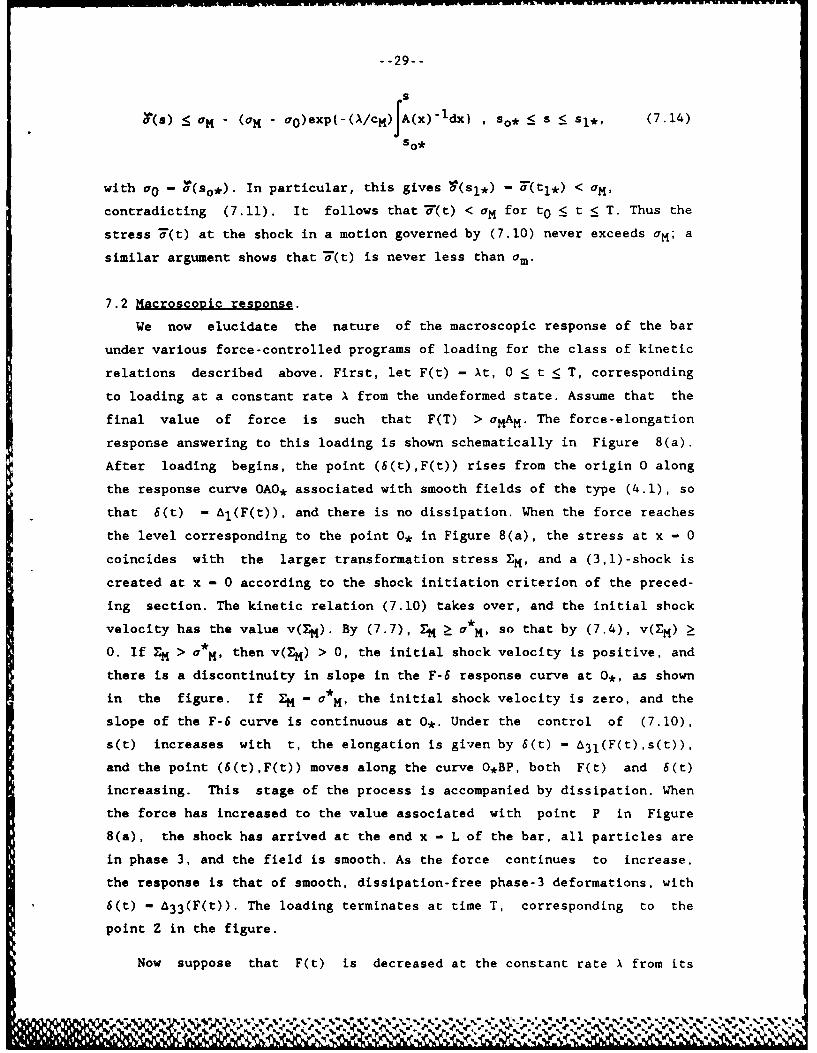
7.2 Macroscopic response.

We now elucidate the nature of the macroscopic response of the bar

under various force-controlled programs of loading for the class of kinetic

relations described above. First, let F(t) - At, 0 < t < T, corresponding

to loading at a constant rate A from the undeformed state. Assume that the

final value of force is such that F(T) > aMAM4. The force-elongation

response answering to this loading is shown schematically in Figure 8(a).

After loading begins, the point (6(t),F(t)) rises from the origin 0 along

the response curve OAO* associated with smooth fields of the type (4.1), so

that 6(t) - Al(F(t)), and there is no dissipation. When the force reaches

the level corresponding to the point 0* in Figure 8(a), the stress at x - 0

coincides with the larger transformation stress EM, and a (3,1)-shock is

created at x - 0 according to the shock initiation criterion of the preced-

ing section. The kinetic relation (7.10) takes over, and the initial shock

velocity has the value v(EM). By (7.7), E a M' so that by (7.4), v(ZM) >

0. If EM > a*H, then v(ZM) > 0, the initial shock velocity is positive, and

there is a discontinuity in slope in the F-6 response curve at 0*, as shown

in the figure. If EM - a'M, the initial shock velocity is zero, and the

slope of the F-6 curve is continuous at 0*. Under the control of (7.10),

s(t) increases with t, the elongation is given by 6(t) - A31(F(t),s(t)),

and the point (6(t),F(t)) moves along the curve O*BP, both F(t) and 6(t)

increasing. This stage of the process is accompanied by dissipation. When

the force has increased to the value associated with point P in Figure

8(a), the shock has arrived at the end x - L of the bar, all particles are

in phase 3, and the field is smooth. As the force continues to increase,

the response is that of smooth, dissipation-free phase-3 deformations, with

6(t) - A3 3(F(t)). The loading terminates at time T, corresponding to the

point Z in the figure.

Now suppose that F(t) is decreased at the constant rate A from its

--30--

largest value F(T) to zero. The response curve at first follows the arc

ZPQ* corresponding to smooth phase-3 fields, and the response is dissipa-

tion-free ; at Q*, the stress at the larger end x - L of the bar has dimin-

ished to the smaller transformation stress Em, and a leftward moving

(3,1)-shock emerges. The sign of v in (7.10) is now negative, s(t), F(t)

and 6(t) all decrease, and the arc Q*CA is traced out as the shock returns

to x - 0, dissipating as it moves. As F(t) decreases to zero from its value

at A, 6(t) - Al(F(t)) again along the arc AO, and the final stage of

unloading takes place without dissipation. The total dissipation in the

loading cycle is of course precisely the area of the hysteresis loop

AO*PQ*.

If the loading rate A were changed, the loading and unloading "yield

points" 0* and Q* would remain the same, but the arcs O*BP and Q*CA

associated with the dissipative portion of the process would change. The

macroscopic response is thus rate-dependent.

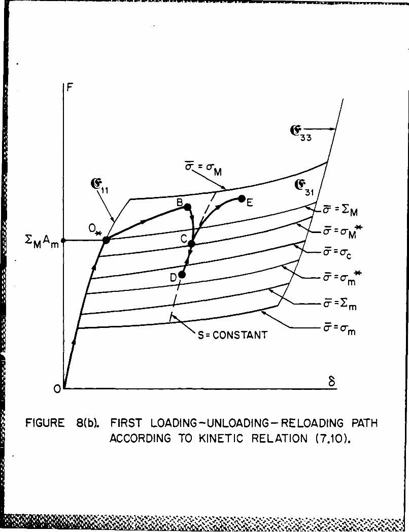
Consider now a modified version of the loading history described above

in which the force F(t), after arriving at the value associated with the

point B in Figure 8(a), is decreased, and then ult.imately increased again.

Figure 8(b) shows the resulting macroscopic response. As before, the

response curve is the arc 00*B during the initial loading phase, the por-

tion O*B being dissipative. When F(t) begins to decrease, v(F(t)/A(s(t))

remains positive at first, and (7.10) requires s(t) to continue to

increase, accompanied by dissipation. During this stage, 6(t) will also

continue to increase, generating the arc BC of the response curve. At the

point C, the stress 7 at the shock has dropped to the value a'M, so that by

(7.4), v(a) - 0 at the corresponding instant. If a*M > a*m in (7.4), and if

F(t) continues to decrease below its value at C, T(t) will remain in the

range for which v(7(t)) vanishes, so that ;(t) - 0 and the shock remains

stationary. During this portion of the unloading process, the corresponding

part CD of the response curve lies along a curve of constant s, and there

is no dissipation. If now the force F(t) is increased, the initial portion

of the reloading process takes place along DC and is dissipation-free. If

the force ultimately increases sufficiently to raise the stress at the

shock to a value greater than a*M, the shock resumes its motion, dissipa-

tion will begin again, and the response curve will proceed along CE. This

particular force history illustrates the occurrence of dissipation-free

unloading with a stationary shock.

--31--

If, during unloading in the last program, the force had been decreased

sufficiently below its value at D, the stress at the shock would diminish

below the value a* causing v(T(t)) to become negative, forcing the shock

to move left. Figure 8(c) shows the macroscopic response curve OO*BFI for

such a force history, together with the response on reloading. The arcs

00*, CE, and GH correspond to dissipation-free periods during the quasi-

static motion.

The macroscopic response of the bar during the loading programs just

described clearly resembles that associated with visco-plastic behavior in

several respects. One feature of the latter kind of behavior that is not

present here is that of permanent strain. By abandoning the requirement am

> 0 in (2.9) and thus considering a stress-strain curve whose local minimum

(Figure 1) corresponds to a compressive stress am, one can introduce

permanent strain into the macroscopic response; see [18].

7.3 Rate-independent behavior.

The form of the kinetic response function sketched in Figure 7(b) sug-

gests consideration of the limiting case in which the function V inverse to

v is a step-function as shown in Figure 9:

P(I) -f EM for i > 0,- (7.15)Em for A < 0,

where EM and Em are the shock initiation stresses, am : Em < ac < EM S aM

and ac is the Maxwell stress. One shows readily that the macroscopic

response produced by the kinetic relation is rate-independent and is of the

form shown in Figure 9. If Em - am and EM - aM , the quasi-static motions

permitted by the kinetic relation are maximally dissipative in a definite

sense; response of this kind is discussed in detail in [17].

7.4 Dissipation-free macrosco2c resonse.

Finally, we note that purely conservative (or dissipation-free)

response of the kind conventionally associated with elastic behaviorresults from choosing the inverse kinetic response function W to be

- c for - < < . (7.16)

--32--

and taking both shock initiation stresses EM and Em to be equal to the

Maxwell stress ac , In this case, the macroscopic response is independent of

past history and is as shown in Figure 10.

!% ° %

REFERENCES

[1] R.D. James, Displacive phase transformations in solids, Journal ofthe Mechanics and Physics of Solids, 34 (1986) 359-394.

[2] R.D. James, Co-existent phases in the one-dimensional static theoryof elastic bars, Archive for Rational Mechanics and Analysis, 72(1979) 99-140.

[3] J.K. Knowles, On the dissipation associated with equilibrium shocksin finite elasticity, Journal of Elasticity, 9 (1979) 131-158.

[4] J.D Eshelby, The continuum theory of lattice defects, Solid StatePhyicsF. Seitz and D. Turnbull, eds.) Vol. 3, Academic Press, NewYor'k, 145P.

[5] J.R. Rice, Continuum mechanics and thermodynamics of plasticity inrelation to microscale deformation mechanisms, in Constitutive Equa-tions in Plastity, (A.S. Argon, ed.) pp. 23-79, MIT Press, Cam-bridge, Massachusetts, 1975.

[6] L.D. Landau and E.M. Lifshitz, Fluid Mechanics, Vol. 6 of Course ofTheoretical Physics, Pergamon, New York, 1959

[7] J.K. Knowles and E. Sternberg, On the failure of ellipticity and theemergence of discontinuous deformation gradients in plane finiteelastostatics, Journal of Elasticity, 8 (1978) 329-379.

[8] R. Abeyaratne, An admissibility condition for equilibrium shocks infinite elasticity, Journal of Elasticity, 13 (1983) 175-184.

[9] M.E. Gurtin, Two-phase deformations of elastic solids, Archive forRational Mechanics and Analysis. 84 (1983) 1-29,

[10] J.L. Ericksen, Equilibrium of bars, Journal of Elasticity, 5 (1975)191-201.

[11] R. Abeyaratne, Discontinuous deformation gradients in the finitetwisting of an incompressible elastic tube, Journal of Elasticity, 11(1980) 42-80.

[12] J.M. Ball and R.D. James, Fine phase mixtures as minimizers ofenergy, to appear in Archive for Rational Mechanics and Analysis,

[13] R.L. Fosdick and R.D. James, The elastica and the problem of purebending for a non-convex stored energy function, Journal of Elastic-JZ, 11 (1981) 165-186.

[14] R.L. Fosdick and G. MacSithigh, Helical shear of an elastic circulartube with a non-convex storea energy, Archive for Rational Mechanicsand Analysis, 84 (1983) 31-53.

[15] S.A. Silling, Consequences of the Maxwell relation for anti-planeshear deformations of an elastic solid, to appear in Journal of Elas-~ticity,

[16] R.D. James, Finite deformation by mechanical twinning, Archive forRational Mechanics and Analysis, 77 (1981) 143-176.

[17] R. Abeyaratne and J.K. Knowles, Non-elliptic elastic materials andthe modeling of dissipative mechanical behavior: an example, toappear in Journal of Elasticity.

[18] R. Abeyaratne and J.K. Knowles, Non-elliptic elastic materials andthe modeling of elastic-perfectly plastic behavior for finite defor-mation Journal of the Mechanics and Physics of Solids, 35 (1987)343-365.

[19] J.R. Rice, On the structure of stress-strain relations for time-dependent plastic deformation in metals, Journal of Applied Mechan-jij, 37 (1970) 728-737.

[20] J.R. Rice, Inelastic constitutive relations for solids: An internal-variable theory and its application to metal plasticitv, Journal Qthe Mechanics and Physics of Solids, 19 (1971) 433-455.

t l % \ % % , '. L LL ,% % ... .'. .. .' . .%. .V '' .''" ,' .

[21] L. Delaey, R.V. Krishnan H Tas and H. Warlimont, Review: Thermo-elasticity, pseudo-elasticity and the memory effects associated withmartensitic transformations, Journal of Materials Science, 9 (1974)1521-1555.

[22] B. Budiansky, J.W. Hutchinson and J.C. Lambropoulos, Continuum theoryof dilatant transformation toughening in ceramics InternationalJournal of Solids and Structures, 19 (1983) 337-355.

[23] J.B. Martin, Plasticity: Fundamentals and General Results, MIT Press,Cambridge, Massachusetts, 1975.

ON-1. .4#0 0*4.*A 0 '0 1.

-vW~lw Mm-.-WW W, -X -m - vq~~f 9wr -

'U z

w

<b 10

b b E

z

a-z

0

CL

b b b L

W. w

b% %

z 60

bi

z-J

z0

LI

LU

I -

Li

0 0

cL

ci

Li

IL

b b

0~ A Wkq 0 W -'

zO--j

CL

0

crN

ojo

b LJ

1-

LU

LLL

EE

-rwr trn*dwwn nn- --

t

*-C x s(t)

O L

FIGURE 3. EXAMPLES OF THE FOUR TYPES

OF TRANSITION INSTANTS t.-, IN (4.7).

% %

3:* a

IL

-J >

LLUfo5

LU

2 E cr.< M

M I bE E I , - N L

NNc

to

b b

z

N z0

0

w

t LU

INI

NN

* -

E A-

Ro410 bEa _gI NLm 0 -e I

0

z

4

00'S

-Jw

0

LL~

U-

LLLills! I'll A I ll0

tow

w0

CLJ

0

L

LL.4

I cn

b b J ' b

E40

z

-; z0

zLL

LUCr-

*p %

F

33

z

T M AmO i - = 'M

0/ -~mAM

0.0*=c-m

=-m

0

FIGURE 8(a). LOADING-UNLOADING PATH ACCORDING TOKINETIC RELATION (7.10)

1 * ioei ~V

F

3

2MArem. =-

a - m0-I

FIGURE 8(b). FIRST LOADING-UNLOADING- RELOADING PATHACCORDING TO KINETIC RELATION (7.10).

- - .. cc

F

33

c- C'mB E1

0 0MMS-- CONSTAN

FIGURE 8(c). SECOND LOADING-UNLOADING-RELOADING PATHACCORDING TO KINETIC RELATION (7.10).

-ma -.

c'

0

~MAM 00

m m

0

FIGURE 9. RATE-..INDEPENDENT DISSIPATIVE

MACROSOPIC RESPONSE.

% ' -6

*,

F

0 33

*FIGURE 10. DISSIPATION -FREE MACROSCOPIC RESPONSE.

UNCLASSIFIEDSECURITY CLASSIFICATION Or THIS PAGE

REPORT DOCUMENTATION PAGE

la. REPORT SECURITY CLASSIFICATION lb RESTRICTIVE MARKINGS

UNCLASSIFIED2a. SECURITY CLASSIFICATION AUTHORITY 3 DISTRIBUTION/AVAILABILITY OF REPORT

2lb. DECLASSIFICATION / DOWNGRADING SCHEDULE UNL IMI TED

4. PERFORMING ORGANIZATION REPORT NUMBER(S) 5 MONITORING ORGANIZATION REPORT NUMBER(S)

TECHNICAL REPORT NO. 1

. NAME OF PERFORMING ORGANIZATION 6o. OFFICE SYMBOL 7a NAME OF MONITORING ORGANIZATION

Calif. Institute of Technology (if applicable) OFFICE OF NAVAL RESEARCH

6r. ADDRESS (City, State, and ZIP Code) 7b ADDRESS (City, State, and ZIP Code)

Pasadena, California 91125 Pasadena, California 91106-3212

ea. NAME OF FUNDING/SPONSORING 8b. OFFICE SYMBOL 9 PROCUREMENT INSTRUMENT IDENTIFICATION NUMBERORGANIZATION (If applicable)

Office of Naval Research N00014-87-K-0117Sr- ADDRESS (City, State, and ZIP Code) 10 SOURCE OF FUNDING NUMBERS

PROGRAM PROJECT TASK WORK UNITArlington, Virginia 22217-5000 ELEMENT NO NO. NO ACCESSION NO

11 TITLE (Include Security Classification)

ON THE DISSIPATIVE RESPONSE DUE TO DISCONTINUOUS STRAINS IN BARS OF UNSTABLEELASTIC MATERIAL

12. PERSONAL AUTHOR(S)Rohan Abeyaratne and James K. Knowles

13a. TYPE OF REPORT 13b. TIME COVERED j14. DATE OF REPORT (Year, Month, Day) 115 PAGE COUNT

TECHNICAL IFROM TO ISeptember 1987 I 5116. SUPPLEMENTARY NOTATION

17. COSATI CODES 18 SUBJECT TERMS (Continue on reverse if necessary and identify by block number)

FIELD I GROUP I SUB-GROUP

19 ABSTRACT (Continue on reverse if necessary and identify by block number)

Some elastic materials are capable of sustaining finite equilibrium deformations with dis-continuous strains. Boundary-value problems for such "unstable" elastic materials oftenpossess an infinity of solutions, suggesting that the theory suffers from a constitutivedeficiency. In the setting of the one-dimensional theory of bars in tension , the presentpaper explores the consequences of supplementinq the theory with further constitutive infor-mation. This additional information pertains to the surface of strain discontinuity andconsists of a "kinetic relation" and a criterion for the "initiation" of such a surface.We show that the quasi-static response of the bar to a prescribed force history is then

fully determined. In particular, we observe how unstable elastic materials can be used tomodel macroscopic behavior similar to that associated with visconlasticity.

20. DISTRIBUTION/ AVAILABILITY OF ABSTRACT 21 ABSTRACT SECURITY CLASSIFICATION

MUNCLASSIFIED/UNLIMITED M SAME AS RPT C3 DTIC USERS UNCLASSIFIED22a. NAME OF RESPONSIBLE INDIVIDUAL 2 b.TELEPHONF (Include Area Code) 22c. OFFICE SYMBOL

J. K. KNOWLES (818) 356-4135 j

DD FORM 1473.84 MAR 83 APR edition may be used until exhausted. SECURITY CLASSIFICATION OF THIS PAGE

All other editions are obsolete. UNC LASS I F I ED

% % % %

tAE IFEREE

F13. I9w'VP

- :D** '