D S EWorking Paper

The Bright Side of MAUP:an Enquiry on the Determinantsof Industrial Agglomeration in the United States

Carlo Menon

Dipartimento Scienze Economiche

Department of Economics

Ca’ Foscari University ofVenice

ISSN: 1827/336X

No. 29/WP/2008

W o r k i n g P a p e r s D e p a r t m e n t o f E c o n o m i c s

C a ’ F o s c a r i U n i v e r s i t y o f V e n i c e N o . 2 9 / W P / 2 0 0 8

ISSN 1827-3580

The Working Paper Series is availble only on line

(www.dse.unive.it/pubblicazioni) For editorial correspondence, please contact:

wp.dse@unive.it

Department of Economics Ca’ Foscari University of Venice Cannaregio 873, Fondamenta San Giobbe 30121 Venice Italy Fax: ++39 041 2349210

The Bright Side of MAUP: an Enquiry on the Determinants of

Industrial Agglomeration in the United States

Carlo Menon London School of Economics

September 2008 Abstract Using county employment data for US and two appositely developed zoning algorithms, I compare the industrial concentration of manufacturing sectors calculated following the standard metropolitan and micropolitan statistical areas definition with two other counterfactuals, obtained by “gerrymandering” the original sample of counties. The methodology allows i) to obtain an unbiased estimate of industrial agglomeration which significantly improves on existing indices, and ii) to provide a ranking of industries according to their responsiveness to labour market determinants of agglomeration. Results show that labour market determinants explain one quarter of the variation of spatial agglomeration across industries. Keywords Industrial Agglomerations;, MAUP, Industrial Concentration JEL Codes O18, R12

Address for correspondence: Carlo Menon

Department of Geography and Environment London School of Economics

Houghton Street London WC2A 2AE, UK

e-mail: c.menon@lse.ac.uk

This Working Paper is published under the auspices of the Department of Economics of the Ca’ Foscari University of Venice. Opinions expressed herein are those of the authors and not those of the Department. The Working Paper series is designed to divulge preliminary or incomplete work, circulated to favour discussion and comments. Citation of this paper should consider its provisional character.

1

1. Introduction

The high degree of spatial concentration of firms belonging to the same

industry is a striking real world fact. A widely accepted theoretical explanation

of its determinants has been proposed more than one century ago by Alfred

Marshall (1890), who identifies the labour market pooling, input sharing and

knowledge spillovers as the main drivers of the process. Empirical evidence,

however, has not been satisfactorily eloquent in assessing the relative

importance of the different determinants.

In this paper, I develop a new methodology aimed at disentangling the

effects of the “labour market” determinants of agglomeration. Starting from an

exploration of the Modifiable Areal Unit Problem (henceforth MAUP), i.e., the

apparently unpredictable dependence of results on the size and the shape of

spatial units, I argue that this variation can rather be interpreted as useful

information, once in command of the process generating the spatial

classification. More specifically, I compare the level of concentration of each

industry calculated using the commuting-defined US metropolitan areas (Core

Based Statistical Areas - CBSAs) against the level of concentration of the same

industry in a counterfactual of randomly aggregated spatial units, arguing that

the industry-specific difference in spatial concentration between the two

datasets is proportional to the importance of the labour market determinants.

The reclassification of the aforementioned Marshallian determinants

under the more general categories of “labour market related” and “non labour

market related” is motivated by the empirical strategy, but it is also relevant for

policy. Examples of labour market determinants may be the need for specific

skills, for low wages, or for an environment where workers can enjoy frequent

interactions with an heterogeneous labour force, or also some local amenities

which make the location particularly appealing for specific groups of workers;

more generally, everything is capitalized by the firm through the labour force

(via lower wages or higher productivity). Examples of non labour market

determinants are input-output linkages between firms, access to local natural

resources, lower prices for inputs other than labour. The aim of this paper is to

2

assess which industries are most dependent on labour market determinants in

their spatial concentration pattern, as opposed to other Marshallian

determinants.

Labour market determinants may have a non-linear, and even non-

monotonic, relationship with the variables that are commonly used to proxy the

input intensity of industries (average wage, total labour compensation over

total value of shipment, capital intensity, etc.). E.g., a particular industry may

target a local endowment of low-wage labour force, another a highly skilled

one. Both the industries may consider labour supply as the most important

determinant of their location, but they completely differ in the average wage

level. Moreover, the hi-skill industry may be capital intensive, which implies

that it allocates a low share of total costs to labour compensation, while the

low-skill one is likely to have a large labour force and thus a bigger share of

labour cost. Alternatively, capital intense production may require also

repetitive and unqualified labour, which translates into a low average wage.

Therefore, results from a cross-industry linear regression of a concentration

index on measures of input intensity can be inconsistent.1 This provides the

main argument for developing a different approach, which does not require to

estimate a priori how industries relate to local labour markets.

Functional areas based on the self-containment of commuting flows are

generally used as an approximation of the spatial extent of single labour

markets. We can therefore assume that commuting-defined areas exhibit the

maximum value (among all the possible spatial classification based on the

same building blocks) of “within homogeneity” and “between heterogeneity”

of labour markets characteristics. At the same time, the effects of the

determinants of agglomeration which are not dependent on the labour market

(i.e., input-output linkages, market access and transport costs, natural

advantages) are not affected by labour heterogeneity; the only spatial

characteristics which matter, in this case, are location and distance. It follows

1 One could theoretically interact industry input intensity with local factor endowments (as done, for instance, by Midelfart-Knarvik et al., 2000), but obtaining the necessary geographic and industrial data is impossible in most of the cases; moreover, one would still need to assume the process is monotonic in the interaction variable.

3

that the amount of concentration of each industry I find using a commuting-

defined area should not be smaller than that found in a comparable dataset of

randomly shaped spatial units (i.e., where the “ceteris paribus” condition holds

for everything except the self-containment of commuting flows), and that this

difference depends on the importance of the labour market determinants for

that industry.

I also contribute to the existing literature by developing a new

technique for correctly estimating the amount of spatial concentration of each

industry. It is widely known that the traditional concentration measures (e.g.,

Gini or Krugman indices) are affected by the “dartboard effect” bias2 (Ellison

and Glaeser, 1997), i.e., the amount of spurious concentration given by the

“lumpiness” of industrial establishment and the discrete classification of the

space. Another, less known, source of bias for concentration indices is

essentially geographic and is given by the arbitrary aggregation (or

disaggregation) of events in a continuous space using exogenously defined

spatial units.

Generally, however, scholars tend to ignore the geographical

component of the bias, limiting themselves to controlling for the industry-

specific plant employment concentration (e.g. Ellison and Glaeser, 1997;

Maurel and Sedillot, 1999). Alternative approaches to the description of the

pattern of industrial concentration are based on Point Pattern Analysis and on a

continuous definition of space (Marcon and Puech, 2003; Duranton and

Overman, 2005). These studies offer a more precise description of the

concentration pattern via the elimination of the discrete spatial unit; but the

latter is often a direct source of data and a natural target for policy, thus the

approach may be limiting in few circumstances.

I propose a different approach, which consists in estimating the “noise”

with a Monte Carlo procedure, and then in filtering out the industry-specific

estimated noise from the estimates of industrial concentration. The vector of

2 The definition comes from the metaphor used by Ellison and Glaeser (1997): if an industry exhibits high concentration of plant employment, then traditional indices will found positive concentration just for a statistical effect, even if the underlying spatial process is completely random (that is, even if one randomly throws plants to a map).

4

industry-specific values of the noise is given by the average concentration

value (as measured by a “raw concentration index”) in a distributions of 1000

random counterfactuals, each of them obtained by i) randomly “shuffling”

plants across the space and ii) randomly aggregating small (not necessarily

contiguous) portions of space (US Zip Code Areas – ZCAs) into spatial units of

the same size of the real ones (CBSAs). Step i) captures the “lumpiness” effect,

and step ii) the geographical bias. By applying this procedure I obtain a

distribution of “spurious concentration” for each industry, which I can easily

use to estimate the amount of “true” concentration (and to test its significance).

Thus, I will assess the level of concentration of each industry in a way

which meets all the criteria listed by Combes and Overman (2004): measures

are comparable across activities and spatial scales, they take a unique known

value under the null hypothesis of no systematic component in the location

process, it is possible to report their significance, the spatial and industrial

classification are controlled for, and the estimation technique is related to

explicit assumptions about theory.

To sum up, I use year 2000 data from the County Business Patterns

(CBP) from US Census to calculate the industrial concentration for the

manufacturing 6-digit sectors in three different settings: in the first one the

spatial unit is the CBSA, in the second one (the noise) it is a random

aggregation of non contiguous ZCAs, and in the third one (the counterfactual)

it is a random aggregation of contiguous counties. The size distribution and the

number of spatial units will be the same in the three datasets. I calculate the

difference between the first two values as an unbiased index of industrial

concentration, and the ratio between the first and the third values as an

estimate of the relative importance of labour market determinants for each

industry.

2. The Determinants of Concentration: Theory and Evidence

Industrial clustering is a striking real world fact and economists have

been speculating on its determinants since more than a century. The principal

5

theoretical reference is Marshall’s Principles in Economics (1890), which

identifies in labour market pooling, knowledge spill-over, and input-output

linkages the drivers of industrial clustering. More recent works formalize

original Marshall’s intuitions, reclassifying the determinants according to a

more theoretical informed taxonomy, composed by matching, sharing, and

learning mechanisms (Duranton and Puga, 2004, who also provide an excellent

survey on the topic). However this and similar contributions refer mostly to the

agglomeration of economic activities as a whole (e.g., why cities exists), while

little is told about the different concentration patterns of individual industries.

Despite the long-established theoretical foundations, empirics of

concentration have not been conclusive so far. Contributions can be separated

into two general categories: the description (or measurement) of the

concentration pattern, and the inference on its determinants at industry level. It

is obvious that if the former is misleading, also the results of the latter are

unreliable.

The first issue has been recently critically surveyed by Combes and

Overman (2004), who effectively point out all the limits of “attempts to

collapse the entire structure of industrial production down to one number that

can be compared across time and across countries” (p. 2855). These limits are

particularly evident in the so-called first generation concentration (and

specialization) indices – namely the Krugman index and Location Gini index –

in the light of the failure to control for the aforementioned “dartboard” bias,

and more generally to meet the target requirements identified by Combes and

Overman.

The second generation indices, i.e., the EG index and similar (Ellison and

Glaeser, 1997; Maurel and Sedillot, 1999), represent a significant

improvement,3 but are still fraught with problems. The Ellison-Glaeser index

for industry k is equal to:

3 Actually this assertion is questionable: although the second generation indices are more theoretical informed, on the other side in few cases a raw employment index is more policy relevant – for instance when we need to assess how much an industry shock translates into a regional shock. In such a case, the only thing that matters is the concentration of employment, irrespectively of the dartboard bias. In the context of this paper the advantages

6

)1(1

1

2

2

ki

i

ki

ik

k

Hx

HxG

−⎟⎠

⎞⎜⎝

⎛−

⎟⎠

⎞⎜⎝

⎛−−

=

∑

∑γ (1)

Where G is defined as

2)( i

kik xsG −= (2)

where s and x correspond to the share of total employment of region i

for industry k and in the aggregate, respectively, and H is the plant employment

Herfindahl index, corresponding to the sum of the squares of the share of

employment of each plant, over the total employment of the industry. The EG

index has the property of controlling simultaneously for the employment

distribution among plants and regions. The authors demonstrate that their index

takes the value of zero under the null hypothesis of random location

conditional on the aggregate manufacturing employment in that region.

Formally, the index derives from a simple model where firms choose their

location according to natural advantages (first order spatial process), and intra-

industry spillovers (second order spatial process). The processes are

observationally equivalent, as both translate into an industry employment share

higher than the aggregate one.

The EG index generated a Pax Romana in the field. However, there are

a few aspects which may still be improved. First, the Herfindahl index takes

into account only the fewness, the average size, and the variance4 of the size

distribution of plants and regions; under the underlying statistical and

theoretical hypotheses, this is sufficient to prove the unbiasedness of the index.

However, more flexible approaches has proved to give rather different results of the second generation indices are evident, but it may be useful to keep in mind and that may not always be the case. 4 As it is widely known, the Herfindahl index can be expressed as 1/n+nσ2, where σ2 is the variance of the employment shares of plants. It therefore depends on the number of plants/regions, their average size, and the variance of their size.

7

(Duranton and Overman, 2005). My methodology will therefore exploit all

available information on the two size distributions without need to rely on any

statistical assumption. Second, equating the probability of a plant to “fall” in a

given region to the region’s aggregate share of employment may not be the

most logical null hypothesis (especially if there are many small regions and

few plants for industry), as the size of plants may be endogenously determined

by the industry pattern of concentration (as shown by Holmes and Stevens,

2002). I will follow a different approach, based on the number of

manufacturing plant sites, rather than on the employment share (which is the

same “null hypothesis” adopted by Duranton and Overman, 2005). Third, the

variance of the employment size of regions is not the only geographical

characteristic which contributes to generate the bias. As Arbia (2001),

Overman and Combes (2004), and Duranton and Overman (2005) clearly

explained, is the whole process of “taking points on a map and allocating them

to units in a box” (Combes and Overman, 2004) that is arbitrary and likely to

introduce a spurious component in the results. This happens because our

“boxes” are generally not regular nor homogenous in both shape and size.

Moreover, in the process we loose all the spatial information embedded in the

data, and distance is collapsed to a binary variable in/out.

Regarding empirical inference, only few contributions provide evidence

on the Marshallian microfoundations of agglomeration economies at industry

level (Ellison and Glaeser, 2001; Rosenthal and Strange, 2001 and 2004).

These studies are based on a linear regression of the EG index on industry-

specific input intensity proxies. Results are not conclusive, however, for many

possible reasons. The first one is data scarcity, both at geographical and

industry level, with the results that the concentration pattern and the input

intensity of industries are extremely difficult to quantify. Generally scholars

use share of total cost as proxies but these are clearly endogenous, as firms

chose locations (and therefore concentrate) in order to minimize costs. This has

been acknowledged (e.g. Rosenthal and Strange, 2001) but not satisfactorily

solved, to the best of my knowledge. Moreover, as already mentioned before, if

the EG index contains a bias, this is transferred into the regression output.

8

Second, the effect of the determinants may be non linear and, more generally,

difficult to parameterize. Third, path dependencies, local idiosyncratic

dynamics, and unobserved factors may play a major role in explaining

industrial concentration. All these elements provide the need for developing an

alternative tool to explore the topic.

3. The MAUP and the Gerrymandering Approach

3.1. The Dark Side

Every geographical area may be divided in a theoretically infinite

number of ways, and economic estimates may present huge variation among

them. Moreover, differently from international comparison – where country

borders have an economic and political meaning that is not comparable with

any other geographic classification – in a sub-national setting researchers face a

variety of administrative and functional divisions – each of them with its pros

and cons – with the result that the choice of the spatial unit is often arbitrary,

even in the rare cases in which it is not constrained by data availability. The

complex and apparently unpredictable variation which the results of

investigations based on “modifiable units” are prone to is called the

“Modifiable Areal Unit Problem” (MAUP). The issue had first been raised by

Gehlke and Biehl (1934), who essentially focussed on the scale problem.

Openshaw and Taylor (1979) provided evidence of how the “shape”

component of the MAUP plays an important role too. In their application, they

generated several distributions of 10,000 random aggregations of the 99 Iowa

Counties, varying the average size of the spatial units and calculating at each

time the correlation between the shares of Republican votes and of elderly

population. The magnitude of the range of values they obtained is extreme (-

0.97 : + 0.99) and increases proportionally to the average size of spatial units.

More recently, Briant et al. (2007) reconsider the role of MAUP with an

application to French data. They perform standard economic geography

analyses (applied to agglomeration, concentration, and trade), using

9

administrative, functional, and random (geometric) spatial units. Although they

find some variations in the results, they eventually reach the conclusion that

“the MAUP induces much smaller distortions than economic misspecification”

(p. 25). Two caveats, however, have to be kept in mind while assessing their

findings: first, the random counterfactual is based on a single iteration, thus is

not possible to test the statistical significance of their results; second, the

French political geography may presents some peculiarities which limit the

extendibility of their conclusions, as the authors themselves acknowledge.

A formal treatment of the topic is due to Arbia (1989), which shows

how the distortions arising from scale and shape effects would be minimized if

the units of analysis were: i) identical, in terms of shape, size and neighbouring

structure; and ii) spatially independent. Given the difficulty of

contemporaneously satisfying the two conditions, in the last years the MAUP

has generally become part of the subconscious of spatial economists and

regional scientists, and has seldom been taken into explicit consideration. In the

rare case it happened, efforts to deal with it have been concentrated on

obtaining a dataset of spatial units which would be “geographically

meaningful” in relation to the enquired phenomenon,5 or in getting rid of the

spatial unit altogether by using a continuous definition of space (e.g., Duranton

and Overman, 2005).

3.2. The Bright Side

My methodology is based on the hypothesis that the variation of

outcomes given by the MAUP has an informative content, which can be

exploited by confronting the properties of differently shaped datasets according

to a known economic rationale. The idea that the MAUP, once under control of

the researcher, may become a powerful tool has already been suggested by

Openshaw (1977), but to the best of my knowledge no applications have been

proposed so far.

5 See Cheshire and Hay (1989) and Magrini (1999 and 2004), for an economic approach; quantitative geography also offer a wide literature on “optimal zoning” of areal units, e.g. Openshaw and Rao (1995).

10

In the present paper I examine the spatial distribution of industries

across the United States, with the aim of assessing the role of labour market

determinants as opposed to technological spillovers, input-output linkages, and

natural advantages. In order to do that, I confront the level of concentration of

each industry in the US “travel-to-work” regions (CBSAs – Core Based

Statistical Areas) against the level of concentration of the same industries in a

distribution of spatial units of the same average size, obtained by randomly

aggregating the same sample of counties which form the CBSAs.

The US Office of Management and Budget defines the CBSAs by

identifying a central county with a significant share of urban population and by

subsequently aggregating the neighbouring counties which have high

commuting linkages with the central one. The aim of this definition is to

contain in the same spatial unit the place of work and of residence of workers.6

The spatial structure of CBSAs – based on a commuting-defined size

and a densely populated centre – is crucial in order to introduce an important

assumption, i.e., the borders of the CBSAs approximate the borders of

individual labour markets. The coincidence of a spatial unit defined on the

maximization of the self-containment of the commuting flows with the concept

of “local labour market” is quite debated in the literature and complicated by

the slippery definition of the latter. The labour market may be defined as a

continuum not only in the spatial, but in almost any of its dimensions

(Cheshire, 1979). Moreover, workers may have different commuting patterns

according to their income and skills. However, some consensus has emerged in

the last years on the comparative advantages of a zoning procedure which

maximizes the self-containment of commuting flows (see Cheshire and Hay,

1989, p. 21-25, for a detailed discussion). The rationale for that rests on the

consideration that the most immediate channel of adjustment and price-clearing

within a spatial labour market is occupational mobility constrained to

6 More information on the CBSA definition can be found in the US Census website (http://www.census.gov/population/www/estimates/metrodef.html) and in the part IX of the Office and Management and Budget Federal Register of 27/12/2000 (OMB, 2000).

11

residential immobility (people change the job but not the house).7 In the

following of the paper I will present an empirical exercise which corroborates

the “labour market homogeneity” hypothesis.

In this context, however, I need a weaker assumption, because the

focus is on a stylized location choice of firms, which may be assumed to be

information constrained. Therefore, there is no need to take into account all the

complex economic interactions between and within labour markets, but – more

simply – the local labour supply “perception” of the firm; and this can

reasonably be approximated by the commuting area. In other words, I simply

assume that a firm which chooses to locate within a given CBSA expects to

face a supply of workers which is spatially constrained by the extent of the

estimated commuting area.

The CBSAs are merely statistical entities, they do not have any political

or administrative meaning and may cross State borders. Hence, if we assume

that the intensity of the “non labour market” determinants of concentration

varies continuously across the physical space,8 it follows that a couple of

contiguous counties shares the same average intensity of input-output linkages,

natural advantages, political environment, market access, etc.; but firms in each

of the two counties are more likely to hire workers living in the CBSAs they

belong to, so the intensity of the action of the labour market determinants will

be different if they belong to a different CBSA.

It follows that two firms A and B located within a given CBSA are

assumed to face the same labour supply irrespectively of bilateral distance

between the two firms, because the closest predominant agglomeration of

workers (the city) is the same. On the other side, two firms C and D situated at

the same distance as A and B, but respectively linked to two different cities by

the predominant commuting flows, face a supply of labour that is partly

different. Consequently, the difference between A-B and C-D in the likelihood

7 Functional areas have then a wider economic meaning, which is essentially given by containing within the same spatial unit the place of work and of residence of the majority of the inhabitants (or workers); but this is not relevant here. 8 Considering that our sample is limited to the counties belonging to the CBSAs, i.e., to counties where a significant level of population or employment is present, the notion of distance we use is corrected for the general spatial distribution of economic activity.

12

to belong to the same industry is proportional to the importance of the labour

market determinants for that industry. Generalizing the argument, if an industry

is highly dependent on labour market characteristics, its heterogeneous

distribution across space will follow the heterogeneous distribution of the

labour endowment. Considering that higher spatial concentration equals higher

heterogeneity among spatial units, it follows that the amount of concentration

determined by the labour market characteristics is expected to be higher in a

dataset in which the spatial units are defined in a way that maximizes the

“within homogeneity” and the “between heterogeneity” of labour market

characteristics, than in any other comparable dataset.

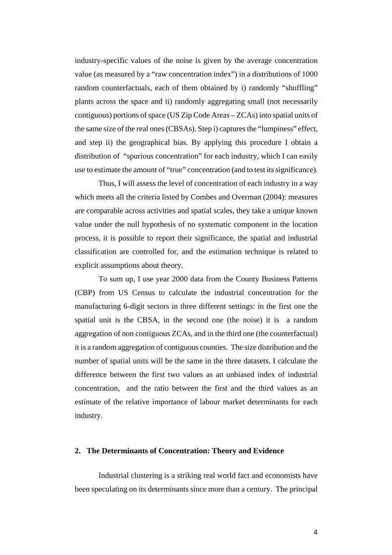
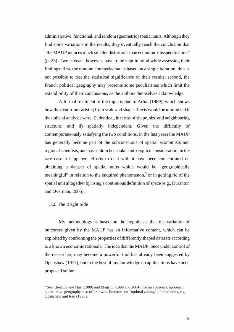
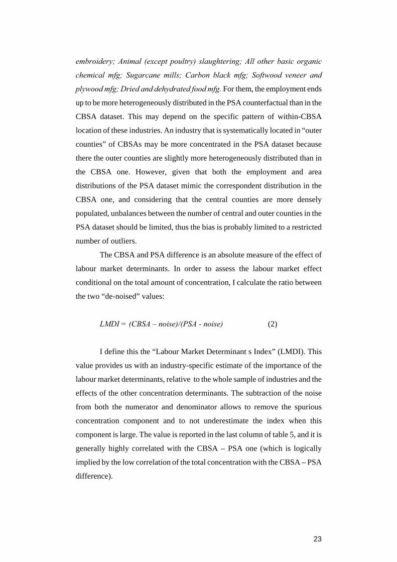
In order to clarify the concept, I introduce a simple example (Figure 1).

Consider a one-dimensional space where there are four cities (1, 2, 3, and 4)

and six industrial districts, belonging to four different industries (A, B, C, and

D). Workers commute from cities to the nearest industrial district, thus forming

the commuting area delimited by the ellipsoids in the upper diagram of Figure

1. Labour is the only input and the location of the different industries is only

due to labour market determinants. A commuting-based classification (like the

CBSAs) will subdivide the space into the four regions reported as rectangular

polygons in the second line of the diagram, thus minimizing the commuting

flows across different spatial units. In the bottom line we report another

random classification, in which spatial units have the same size but the

commuting flows are not taken into account. It immediately appears from the

example that the amount of concentration we can measure using the

commuting-based spatial classification is bigger than what we would find using

any other spatial classification.

The methodology may recall the so-called “regression discontinuity

approach”, which has recently been applied in a geographical setting by

Holmes (1998) and Duranton et al. (2006), among others. However the

apparent analogy is misleading, because the discontinuity I exploit in this case

is only approximate, given that we expect that some commuters will cross

CBSAs borders. It is probably more useful to think of the CBSAs as the spatial

classification which minimizes the cross-unit commuting flows.

13

In order for my methodology to be meaningful, I need to provide

evidence that the CBSA classification presents similar characteristics to the

stylized example. More specifically, the consistency of the methodology

requires that (i) CBSAs have a highly populated centre and a set of outlying

counties which are lower populated, where workers commute to and from; and

(ii) almost the totality of the population lives and work in the same CBSA (but

generally not in the same county), even those who reside close to the CBSA

border.

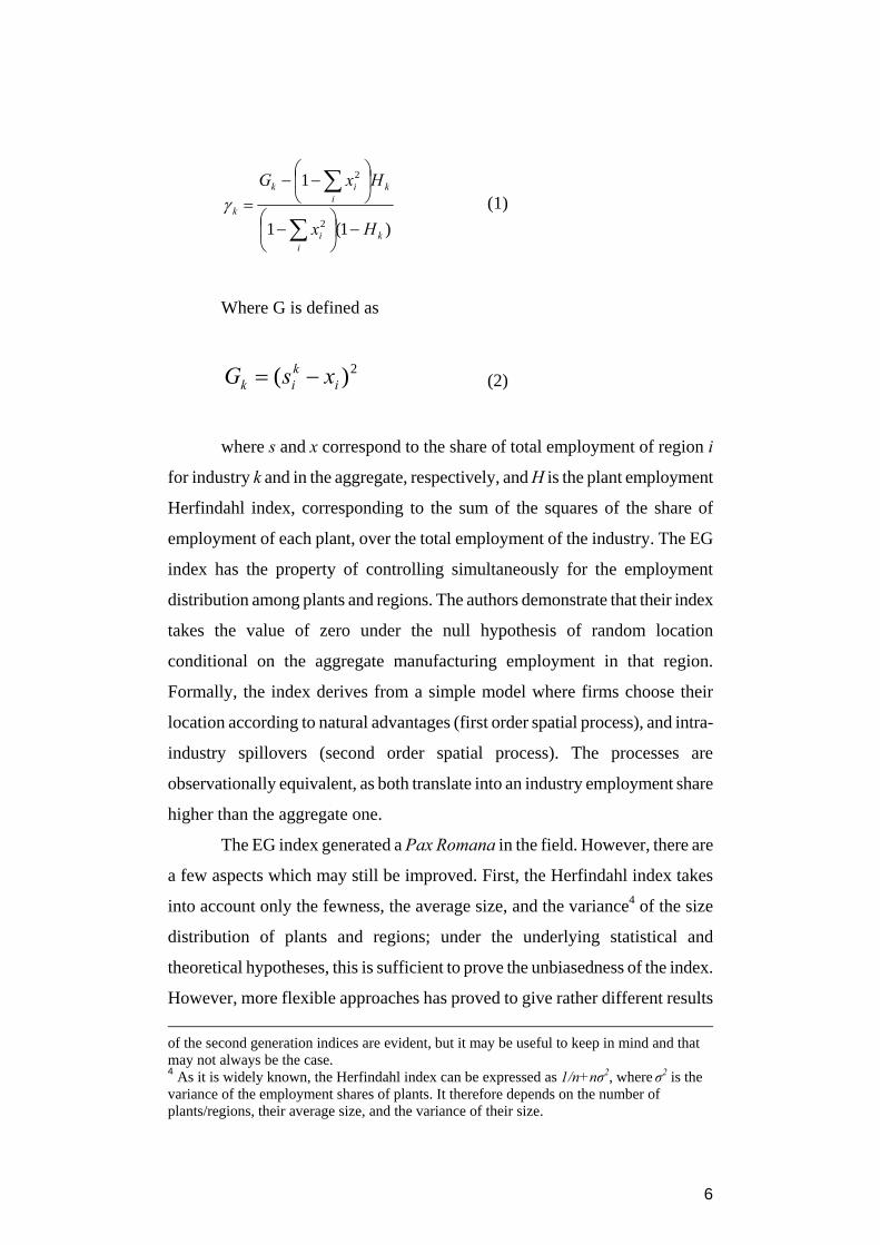
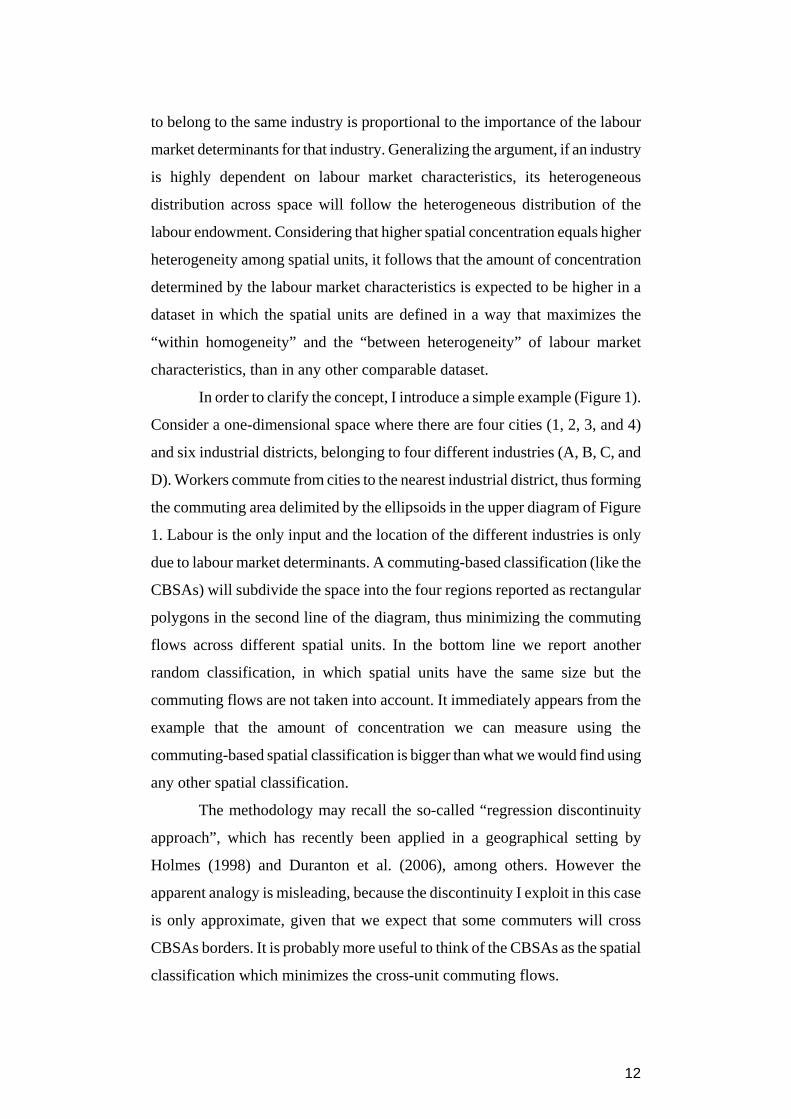
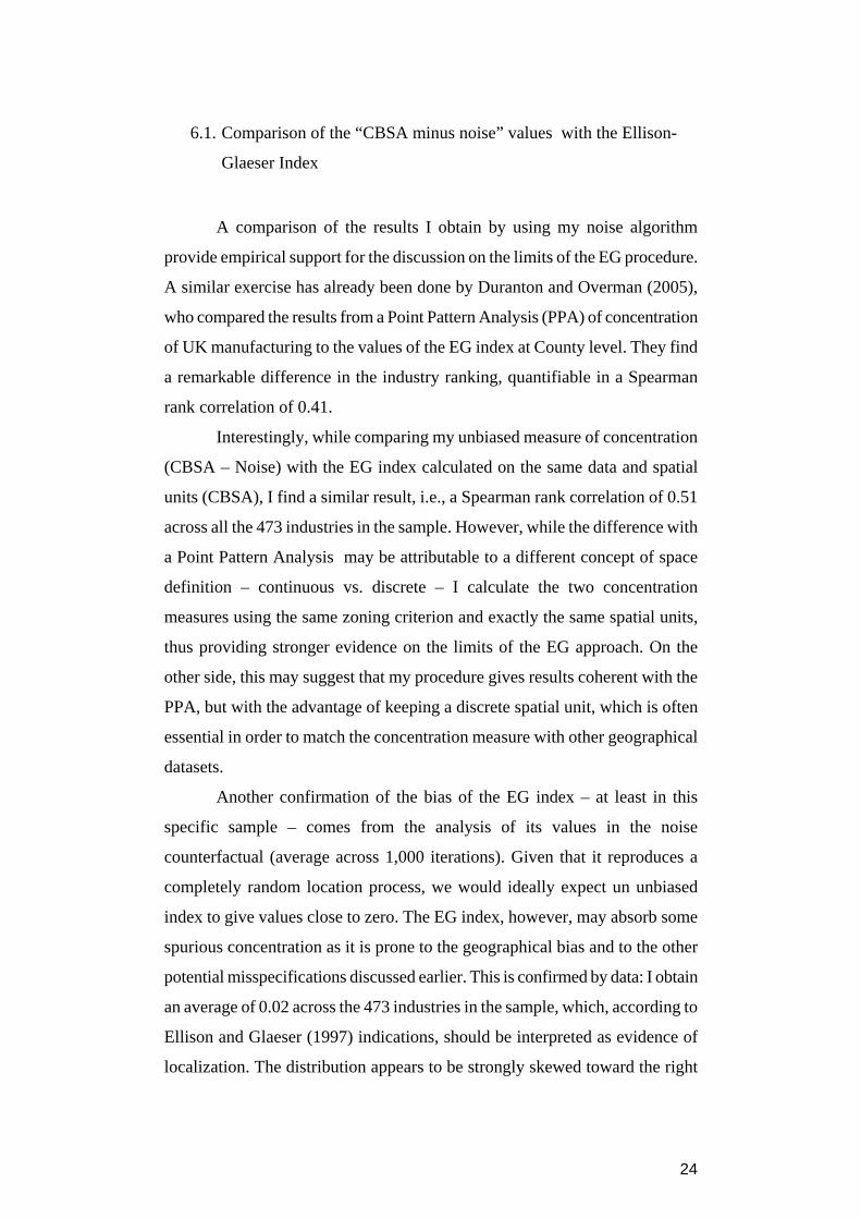
The first condition is given by the definition properties of CBSAs,

which are identified around an urban centre and comprehend the neighbouring,

external counties. In the map in Figure 2 I report the CBSA borders layer

together with a map of populated places; the map clearly shows a common

pattern of urbanization in the central area of CBSAs.

To test the second condition, I used journey-to-work data from the

2000 Census, with the result that only the 9% of employees living in a CBSA

work outside the same CBSA where they reside. On the other side, the 25% of

workforce resident in a CBSA commute outside the County they reside in. This

confirms that CBSAs truly contain the commuting flows, and, at the same

time, there is a significant cross-county commuting activity.

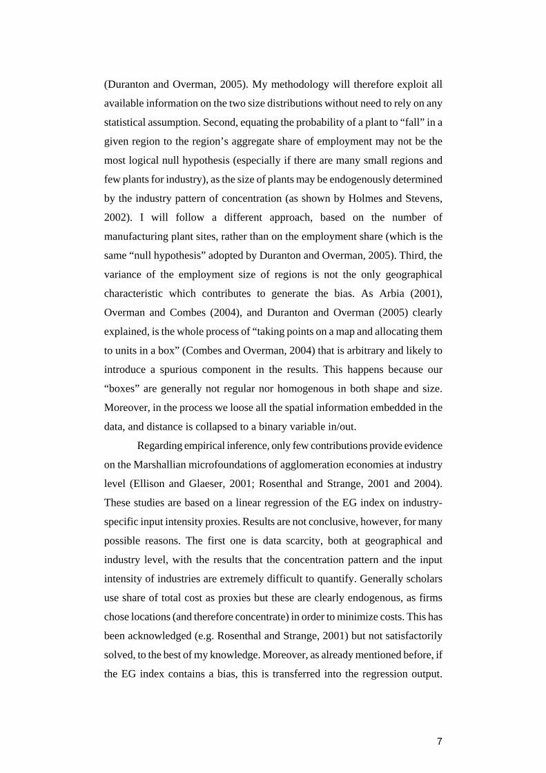
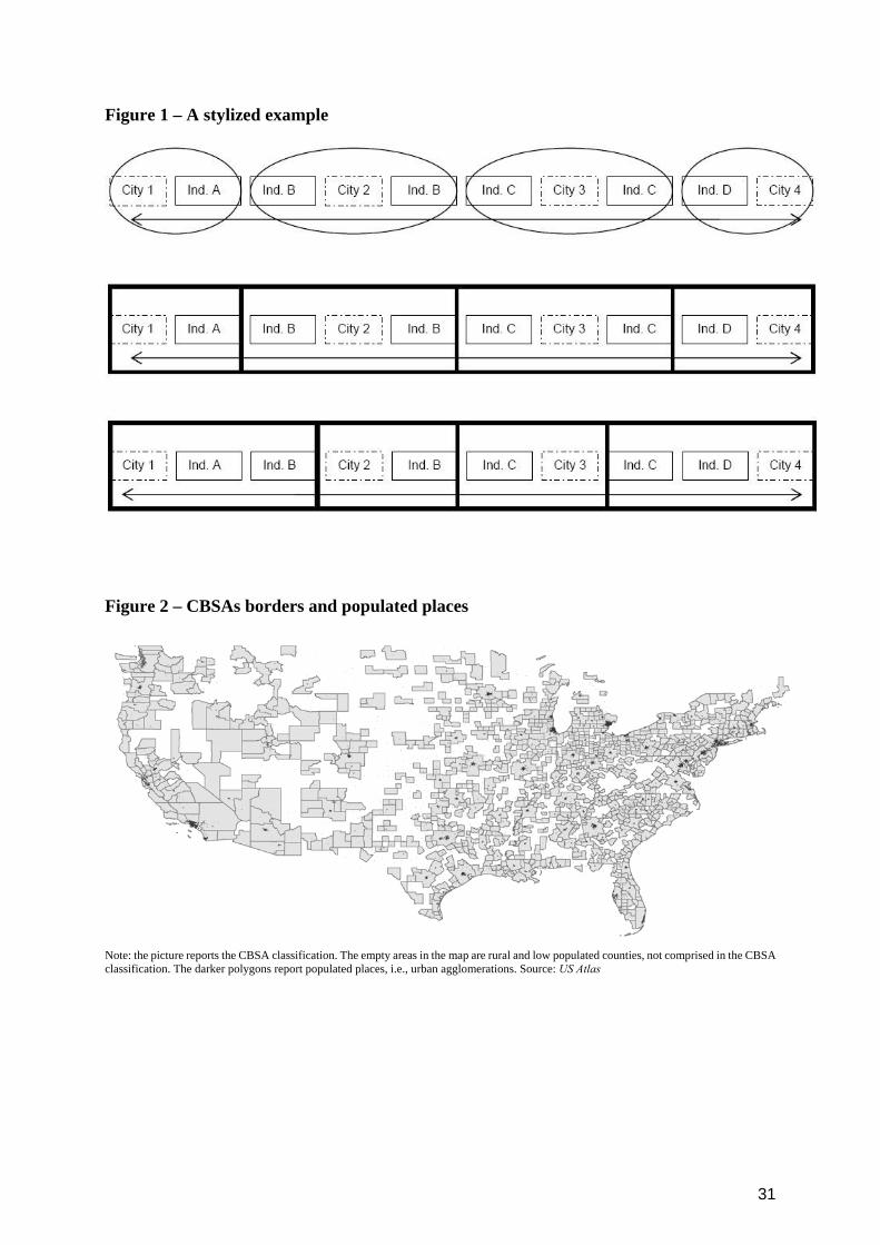
3.3. A Real World Example

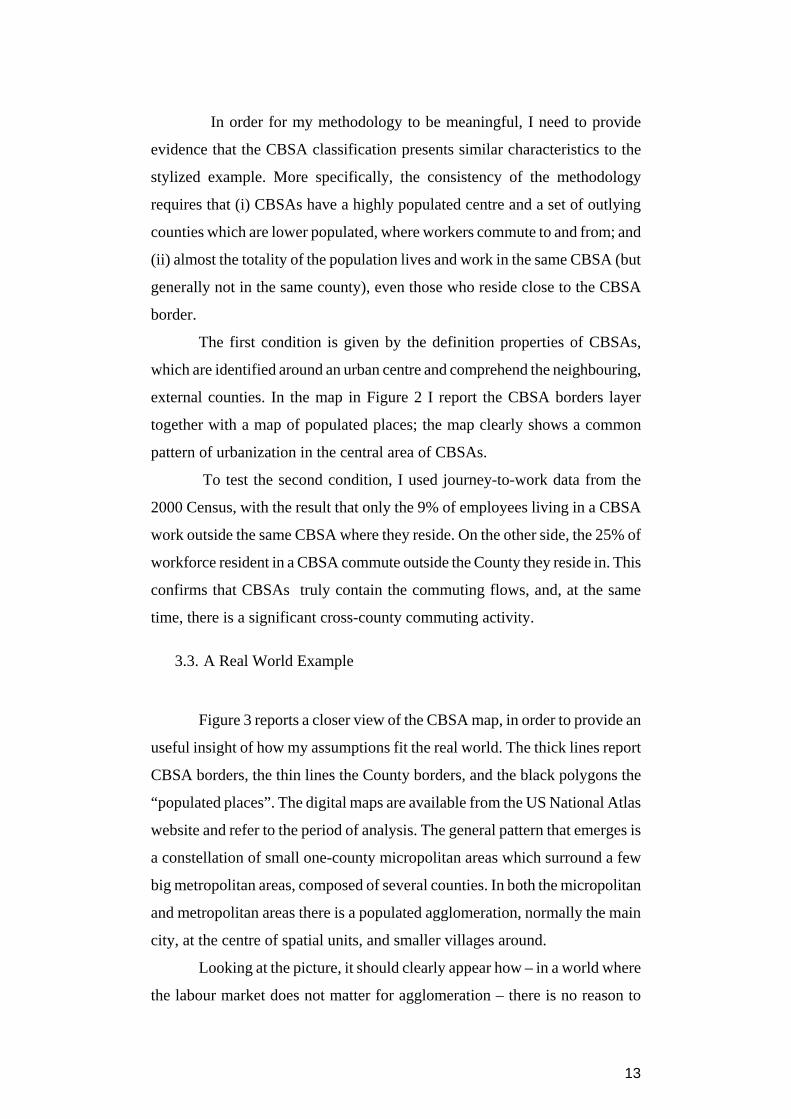
Figure 3 reports a closer view of the CBSA map, in order to provide an

useful insight of how my assumptions fit the real world. The thick lines report

CBSA borders, the thin lines the County borders, and the black polygons the

“populated places”. The digital maps are available from the US National Atlas

website and refer to the period of analysis. The general pattern that emerges is

a constellation of small one-county micropolitan areas which surround a few

big metropolitan areas, composed of several counties. In both the micropolitan

and metropolitan areas there is a populated agglomeration, normally the main

city, at the centre of spatial units, and smaller villages around.

Looking at the picture, it should clearly appear how – in a world where

the labour market does not matter for agglomeration – there is no reason to

14

expect that the CBSA classification would better match the clustering of

economic activities than any other random aggregation of counties. For

instance, if in the North and South parts of the Indianapolis CBSA (at the

centre of the picture) we register the presence of plants of the same industry

and this industry is not present in Anderson, Columbus and Bloomington

(neighbouring CBSAs on the southern side), then this is because of – according

to my previous hypothesis – a specific need of that industry for the labour force

residing in Indianapolis. Conversely, if firm location is driven by the need to

supply another firm in Indianapolis, it can easily be located in Columbus or in

Bloomington, because the only thing which matters in this case is the distance

– there is no reason for this firm to prefer to locate inside the commuting area

of Indianapolis, everything else being equal.

Of course there may be many other unobservable and idiosyncratic

factors driving the firm location but, in a sample of 876 spatial units and more

than 320,000 manufacturing plants, a general pattern should emerge, where the

difference of concentration between the CBSA and a random classification is

related to a “labour market determinants” story. This is, in a nutshell, the

meaning of my work.

The reader may argue that the methodology is affected by a reverse

causality problem, that is, the commuting flows are determined by industrial

clustering and the labour market areas are shaped after the industrial clusters,

rather than being their determinant. I think that this may seldom be the case, as

I am considering only the manufacturing sector, which employs less than the

20% of the workforce, while the commuting flows are calculated on the whole

sample of workers; moreover, often commuting patterns are determined by

exogenous factors, like physical geography or long term investments in

commuting infrastructures.

However, even it were the case, it would not affect the causal linkage

that I am inferring here: the fact that the commuting flows follow industries’

location does not necessarily imply that they come from the same origin, which

is implied by being within the same CBSA. The evidence that they come from

the same origin, i.e., that a given industrial cluster is drawing workers from a

15

single labour market, and that this systematically happens over a big sample of

spatial units, is, in my opinion, difficult to explain with a causality going on the

opposite direction respect to what I assume in this paper.

4. Data

I use six-digit NAICS employment data for Zip Code Areas (ZCAs) and

Counties in the year 2000, freely available from the County Business Patterns

(CBP) of US Census Bureau, in the form of the dataset collected by Prof.

Thomas Holmes, University of Minnesota, and freely downloadable from his

website.9 I also use a shape file from the National Atlas of the United States

and the Luc Anselin’s GeoDa software10 to calculate a first order rook

contiguity matrix11 needed by the PSA algorithm (described in the next

section).

Because of confidentiality issues, in the CBP database many

employment records are reported only in approximated form, i.e., we only

know the size class of the plant. There are various ways to overcome this

problem (see Isserman and Westervelt, 2006, for a survey). As I do not need a

precise locality-specific estimate, I followed the most straightforward route: I

ascribed to every plant the average employment of the class it belongs to (as

done, for example, also by Holmes and Stevens, 2004). Another minor problem

is given by the fact that ZCAs employment data over 1000 employees are

merged in only one class, instead of four as it is in counties data. In order to

obtain comparable data (and, again, considering that the exact estimate of the

employment of each ZCA is not relevant here), I attributed to ZCAs the

distribution of employment class size of the counties data (industry-wise).

From the 3079 counties composing the Continental US (therefore

excluding the States of Alaska, Porto Rico and Hawaii) I selected the records 9 http://www.econ.umn.edu/~holmes/data/CBP. The dataset is described in Holmes and Stevens (2004). 10 Freely downloadable from https://www.geoda.uiuc.edu/ 11 A first order rook contiguity matrix is a symmetric, square NxN matrix, where N is the number of spatial units, in which the element mk is equal to 1 if region m and k share a common border (longer than one pixel in the map), and equal to zero otherwise.

16

of the 1734 counties which are included in the 2000 standards Core Based

Metropolitan and Micropolitan Statistical Areas (CBSAs). From these I

eliminated 26 Micropolitan Statistical Areas which are isolated, i.e., do not

share any border with other CBSAs and therefore would not show any

variability among the random aggregations. I end up with a dataset of 1707

counties which account for the 97% of the total (continental) US population,

and form 876 CBSAs, of which 306 are Metropolitan Statistical Areas and 570

are Micropolitan Statistical Areas. The definition procedure of Metropolitan

and Micropolitan areas is exactly equivalent, but for the latter the population of

the core county has to be smaller than 50,000. However, the overwhelming

majority of Micropolitan Statistical Areas are composed by only one county,

as a consequence of the fact that the commuting flows with the neighbouring

counties are limited.

The same selection of the US territory is applied to the ZCAs dataset,

using the ZCAs-counties geographical equivalence list, also available in Prof.

Holmes website.12

5. Building the Counterfactuals

5.1. The Noise

As I mentioned earlier in the paper, the amount of concentration

detected using raw employment concentration indices is affected by the

“dartboard effect”, i.e., the bias due to the interaction of the “lumpiness” of

industrial establishments and of the discrete classification of space.

Trying to eliminate the bias without renouncing to a discrete

classification of space may be extremely complex and beyond the scope of the

present paper. It is relatively easy, instead, to create a counterfactual where the

amount of concentration measured by a raw concentration index is totally

12 As explained in the website, in few cases ZCAs can cross counties boundaries. Therefore, our selection may introduce a difference between the ZCAs dataset the CBMSA one. However the difference in total employment between the two datasets after the selection is extremely small (0,3%), which seems to be a negligible difference.

17

spurious, i.e., is given only by noise, in order to have an estimate of the bias

specific to the given joint combination of the industry and spatial

classifications.

Therefore, I apply a simple technique which exploits all the information

contained in the plant employment distribution and in the spatial classification

system. My approach consists in composing a distribution of 1000 datasets,

each of them created by applying the following two-step algorithm to the

original sample of plants under analysis:

a) The plants are “shuffled” across ZCAs (Zip Code areas, the

smallest spatial units at which industry data are available), simulating a

scenario where plant location is random given the spatial distribution pattern of

all manufacturing plants. This means that every ZCA ends up with a random –

in term of employment and industry – sample of plants, but with exactly the

same number of plants it originally had.

b) The ZCAs are randomly aggregated – without any contiguity

constraint – into bigger spatial units. The number of these spatial units is

equivalent to the number of CBSA and every time a new spatial unit is created,

its maximum employment size is drawn (without replacement) from the actual

CBSA size distribution, in order to mimic the total employment distribution of

the CBSA dataset. This step is meant to absorb the geographical bias embedded

in the CBSA dataset, by reproducing an equivalent spurious aggregation of

points into comparable “boxes” deprived of any spatial meaning (internal

connectivity).

At every iteration, 13 a raw concentration index (the G concentration

index) end the EG are calculated and stored. At the end of the process we

obtain a distribution of values of the indices for each industry. Interestingly, for

many industries the average G values are definitely high, while the values of

the EG index are generally close to zero, but with significant exceptions,

13 The assignment of plants to PSAs is a slow procedure – it takes around nine minutes with a standard PC. Repeating it 1000 times will take around 150 hours. Therefore, in order to speed up the algorithm, the step b) is repeated only every 50 iteration. However, the random variation of the results at every iteration is assured by the reshuffling of the plants in step a).

18

especially for industries with a small number of establishments. A more precise

description of the “noise pattern” is reported in the next section.

5.2. The Pseudo Statistical Areas (PSAs)

In order to obtain a relative estimate of the importance of the labour

market determinants for each industry, I need a counterfactual in which the

spatial units are in all comparable to the CBSAs, except for the containment of

the commuting flows. This implies two main requirements: i) the “Pseudo

Statistical Areas” (PSAs) must be internally connected, and ii) they must

follow the same size distribution of the CBSAs (in terms of total employment

and area).

Therefore, I composed an algorithm14 which randomly assigns the 1707

counties to 876 internally connected spatial units (every county which is going

to be added to a PSA must be contiguous to at least one of the counties already

composing the PSA). Its functioning can be summarized as follows: for every

county that has not been assigned already, a random neighbour is chosen and

added to a PSA-to-be. A vector including all the neighbours of the two counties

is then created, from which a random contiguous county is chosen and included

to the PSA-to-be. The process continues until the size and employment limit is

reached, or all the counties around the PSA-to-be are assigned. In order to

maximize the degree of internal connectivity, and therefore to avoid to shape

PSAs as long rows of counties, the likelihood for a county to be added to a

PSA is exponentially proportional to the number of contiguous counties

already composing that PSA. For instance, if an unassigned county i is

surrounded by counties which have already been assigned to the forming PSA,

its probability to be assigned is much higher than it is for a county that has

only one contiguous neighbour already assigned to the forming PSA.15

14 The algorithm has been developed by the author and compiled in Matlab® language. Original scripts and more information on its functioning are available on request. Although many contributions have already been proposed on Automated Zoning Procedure (since, e.g., Openshaw 1977), to the best of my knowledge none of them satisfies the properties which I need in this case. 15 The neighbour vector is sorted in decresing order according to the number of times every county is repeated; then a random number is drawn from an exponential distribution with

19

The algorithm is also aimed at closely mimicking the employment size

distribution of CBSAs. This is obtained by imposing to every forming PSA a

total employment limit drawn (without replacement) from the actual CBSA

size distribution. For the bigger PSAs, the limit may not be reached, because

contiguous counties have already been assigned. To avoid that, at every

iteration the twenty biggest PSAs are the first to be composed, aggregating

random counties around the twenty biggest counties.

Although there is a clear trade-off in replicating the size distribution

without limiting the randomness of the aggregation, on average the moments of

the PSA distribution are close to the ones of the CBSA distribution (Table 1,

first two rows). While the focus is prevalently on the employment distribution,

the algorithm contains also some instruction aimed at replicating the CBSA

area distribution (Table 1, third and forth rows). The joint replication of both

the distributions is important for two reasons: first, it avoids that the difference

in concentration between the CBSA and PSA dataset contains a spurious

component due to a different size distribution; second, it also contributes to

keep the distributions of central and outlying counties across spatial units

similar in the two datasets. In fact, as central counties are much denser

populated than the outlying ones, a different repartition of them would

necessarily end up in a different employment or area distribution.

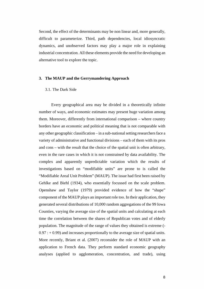
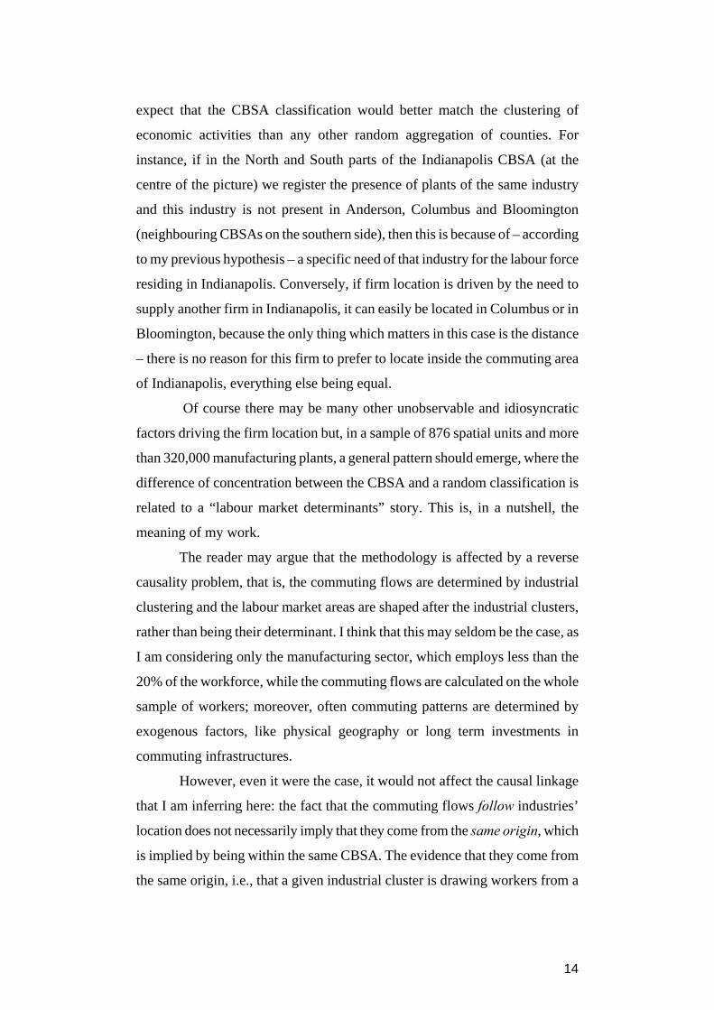
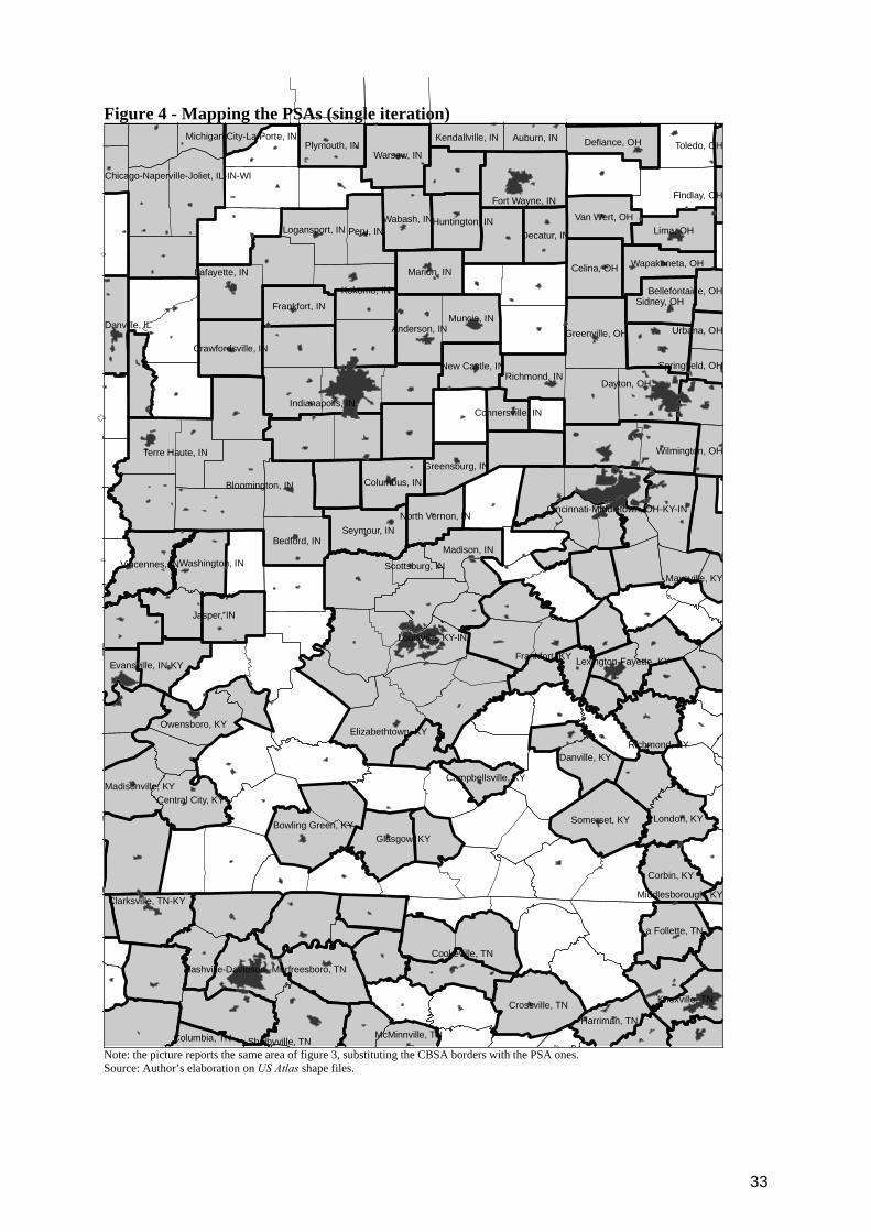
The outcome of a single iteration of the algorithm are visualized in

Figure 4, which reports the same area of Figure 2, substituting the CBSAs’

borders with the PSAs’ ones. The picture shows how the size and the shape of

the spatial units are extremely similar to the original CBSA classification.

Moreover, there are two other reasons which support the robustness of the

results to potential isolated “strange geometries”: first, they would generate a

bias only for industry with a significant share of plants located in that area;

second, and most important, the algorithm executes 1000 iterations, which

implies that to have a bias we would also need the “strange geometries” not be

the lambda parameter equal to three (thus skewed to the left) and bounded by the length of the vector of counties. The random number correspond to the position of the chosen county in the vector; lower is the number, more frequently the county is repeated in the vector. This implies that counties which are repeated most are more likely to be selected.

20

created always in the same location. At every iteration, a raw concentration

index (the G index, defined in the following section) is calculated and stored.

As I mentioned earlier in the paper, I assume that the PSA

counterfactual will be more heterogeneous in terms of labour market

characteristics than it is in the CBSA dataset. I did a simple exercise to test this

assumption: I calculated the coefficient of variation of an immediate proxy of

labour market characteristics – the unemployment rate – in the CBSA and PSA

dataset. In the CBSA dataset the value is equal to 0.377. In 1000 iterations of

PSA dataset I obtain a mean of 0.331, a 90th percentile of 0.348, and a

maximum of 0.366. It implies that the variation of the unemployment rate is

higher in the CBSA dataset than in any of the 1000 counterfactuals, which in

turn means that the requirement of a significantly bigger level of “between

heterogeneity” of labour market characteristics is satisfied.

6. Results

For every industry, my “raw” results consist of the G values, calculated

following the specification reported in (2), for three different groups of

analysis: the CBSAs (a single value for each industry), the PSAs (random

aggregation of contiguous counties, distribution of 1000 values for each

industry), and the “noise” (random aggregation of non necessarily contiguous

Zip Code Areas, distribution of 1000 values for each industry).

The meaning of these values is the following: the CBSA values at net of

noise report the maximum, unbiased amount of concentration given by the

action of all the determinants, while the PSA values at net of the noise should

be smaller, because the effect of the labour market determinants is lower. The

first value is calculated as the difference between the CBSA values and the

average values of the “noise” distribution, while the second one is the

difference of the average values of the two respective distributions (the PSA

one and the noise). I also test the hypothesis that this difference is statistically

null and I report the p-value of the test.

a) Noise: the values of the estimated “noise” provide extremely useful

information for assessing the bias of the concentration index (Table 2). A first,

21

striking result is that the noise is extremely “loud”: the average value of the G

across the 473 manufacturing industries is 0.032, which in previous studies

based on the value of that index would have been interpreted as a remarkable

signal of concentration (with the caveat, however, that the small dimension of

our spatial units and the highly detailed industrial classification partly

contributes to generate big values).

b) CBSAs minus noise: 298 out of 473 manufacturing industries

present a concentration at the CBSA level that is not compatible with the

“noise” counterfactual at 5% level of confidence (215 at 1% level). On the

contrary, only three industries exhibit a 5% significant negative value

(Magnetic and optical recording media mfg; Biological product mfg; Quick

printing). The most concentrated industries, once the noise is eliminated, are

“Jewelers' material & lapidary work mfg”, “Sugarcane mills” and “Women's,

girls' cut & sew dress mfg” . The Spearman rank correlation with the EG

calculated on the same data and spatial classification is equal to 0.51.

Therefore, there is a significant positive correlation, but the matching is far

from being complete. Overall, my methodology seems to add some precision to

the estimate, while the EG index does not eliminate the risks of misleading

estimates for few industries, as shown in Table 2.

c) CBSA minus PSA: this difference is uninformative in its absolute

value, because we cannot know how much of the labour market determinants

effect is absorbed by the PSAs definition, given that it is a random

counterfactual; but we can plausibly assume that it is a share of the total effect,

and that it is constant across industries. A closer examination reveals that the

latter assumption is much weaker than it may appears: the effect absorbed by

the PSAs definition depends on how much the PSAs are geographically similar

to the CBSAs, which in turn affect the values of all the industries in the same

way. Considering that every industry has many plants in many locations, the

space under analysis is the same for all the industries, and the values I use are

averaged across 1000 iterations, the assumption is completely plausible.

An extremely simple formalization may clarify the meaning of the

value. Let’s define the total concentration of industry k in the CBSAs dataset as

22

kkk baX +=

where a and b are the effect of labour and non labour market determinants,

respectively. Let’s then define the total concentration of industry k in the PSAs

dataset as

kkk bmaZ +=

where m is the unknown (but constant across industries) share of labour market

effect captured by the PSA definition. It follows that the difference between the

concentration in the CBSA-PSA dataset, industry-wise, is equal to:

kkkkk jmaaZX =−=−

which is directly proportional to a and is the value I will analyse.

The sign of the CBSA-PSA difference16 is significantly positive at the

5% level in 125 cases (71 at 1%). It means that for around one quarter of

manufacturing industries the level of spatial concentration given by the CBSA

classification is significantly bigger (i.e., the industry employment has a more

heterogeneous distribution across space) than when we use the PSA

counterfactual.

Table 5 reports the first 50 industries according to the CBSA-PSA

value, limited to the sample of industries with a 5% significant difference both

in the CBSA-PSA and CBSA-noise difference. Interestingly, these industries

do not show an immediate clear similarity in labour or skill intensity: both hi-

tech and labour-intensive industries are in the list. E.g., among the first ten

industries in the ranking, we find a few textile industries, as well as space

vehicle manufacturing and optic fibre manufacturing. The hypothesis of a non

monotonic relationship between input intensity and spatial concentration is thus

validated, and confirms the advantages of a non parametric approach.

There are also few industries for which the CBSA-PSA difference is

significantly negative: they are 23 in total, but only nine if the analysis is

restricted to the industries with a 5% significant CBSA-noise difference. These

nine industries are: Electrometallurgical ferroalloy product mfg; Oil and gas

field machinery and equipment mfg; Petrochemical mfg; Schiffli machine

16 From this point on, every mention of Noise and PSA values refers to the average value across 1000 iterations of the zoning algorithm.

23

embroidery; Animal (except poultry) slaughtering; All other basic organic

chemical mfg; Sugarcane mills; Carbon black mfg; Softwood veneer and

plywood mfg; Dried and dehydrated food mfg. For them, the employment ends

up to be more heterogeneously distributed in the PSA counterfactual than in the

CBSA dataset. This may depend on the specific pattern of within-CBSA

location of these industries. An industry that is systematically located in “outer

counties” of CBSAs may be more concentrated in the PSA dataset because

there the outer counties are slightly more heterogeneously distributed than in

the CBSA one. However, given that both the employment and area

distributions of the PSA dataset mimic the correspondent distribution in the

CBSA one, and considering that the central counties are more densely

populated, unbalances between the number of central and outer counties in the

PSA dataset should be limited, thus the bias is probably limited to a restricted

number of outliers.

The CBSA and PSA difference is an absolute measure of the effect of

labour market determinants. In order to assess the labour market effect

conditional on the total amount of concentration, I calculate the ratio between

the two “de-noised” values:

LMDI = (CBSA – noise)/(PSA - noise) (2)

I define this the “Labour Market Determinant s Index” (LMDI). This

value provides us with an industry-specific estimate of the importance of the

labour market determinants, relative to the whole sample of industries and the

effects of the other concentration determinants. The subtraction of the noise

from both the numerator and denominator allows to remove the spurious

concentration component and to not underestimate the index when this

component is large. The value is reported in the last column of table 5, and it is

generally highly correlated with the CBSA – PSA one (which is logically

implied by the low correlation of the total concentration with the CBSA – PSA

difference).

24

6.1. Comparison of the “CBSA minus noise” values with the Ellison-

Glaeser Index

A comparison of the results I obtain by using my noise algorithm

provide empirical support for the discussion on the limits of the EG procedure.

A similar exercise has already been done by Duranton and Overman (2005),

who compared the results from a Point Pattern Analysis (PPA) of concentration

of UK manufacturing to the values of the EG index at County level. They find

a remarkable difference in the industry ranking, quantifiable in a Spearman

rank correlation of 0.41.

Interestingly, while comparing my unbiased measure of concentration

(CBSA – Noise) with the EG index calculated on the same data and spatial

units (CBSA), I find a similar result, i.e., a Spearman rank correlation of 0.51

across all the 473 industries in the sample. However, while the difference with

a Point Pattern Analysis may be attributable to a different concept of space

definition – continuous vs. discrete – I calculate the two concentration

measures using the same zoning criterion and exactly the same spatial units,

thus providing stronger evidence on the limits of the EG approach. On the

other side, this may suggest that my procedure gives results coherent with the

PPA, but with the advantage of keeping a discrete spatial unit, which is often

essential in order to match the concentration measure with other geographical

datasets.

Another confirmation of the bias of the EG index – at least in this

specific sample – comes from the analysis of its values in the noise

counterfactual (average across 1,000 iterations). Given that it reproduces a

completely random location process, we would ideally expect un unbiased

index to give values close to zero. The EG index, however, may absorb some

spurious concentration as it is prone to the geographical bias and to the other

potential misspecifications discussed earlier. This is confirmed by data: I obtain

an average of 0.02 across the 473 industries in the sample, which, according to

Ellison and Glaeser (1997) indications, should be interpreted as evidence of

localization. The distribution appears to be strongly skewed toward the right

25

hand side, which means that the overestimate is particularly high for few

industries (Table 4). Overall, 102 industries present a value bigger than 0.02,

which implies that the bias is substantial for more than one fifth of industries.

Therefore, the Noise counterfactual can provide the basis for further research

on the distribution of the EG index under the null hypothesis of random

location pattern.

6.2. Analysis at 4-digit level

In this section I present the results obtained using a wider industry

classification, i.e., the 86 manufacturing sectors reported at the 4-digit industry

level. There are three main reasons why this may be useful: first, the 6-digit is

an extremely detailed classification and results, although very informative, may

be biased by the presence of few peculiar sub-sectors, which may behave as

outliers. Second, the sectors reported in CBP refer to the prevalent activity of

the plants; it is likely that some plants are actually multi-product, thus, again, a

too detailed classification may be misleading. Finally, the analysis at a higher

level of industry classification disclose also new information per se.

The results – reported in table 6 – are coherent with the 6-digit analysis.

The Spearman rank correlation between the G index at 4 and 6 digits is positive

and significant for all the three different datasets (CBSAs, PSAs, Noise). 31,

out of 86, manufacturing sectors exhibit a positive and significant (at 5%)

CBSA – PSA difference, while the CBSA – Noise difference is significantly

positive in 74 cases.

Similarly to the 6-digits analysis, the top sectors in the CBSA-PSA

ranking do not show a linear dependence on labour input intensity, and a mix

between low and high skill activities emerges. Again, it would be extremely

complex to recognize such a pattern with a parametric analysis.

6.3. Does the labour market matter for concentration?

In order to assess to what extent the concentration driven by labour

market determinants explains the general pattern of concentration, I regress the

26

index reporting the total amount of concentration (CBSA – Noise) on the

estimation of the labour market effect (CBSA – PSA). A positive and

significant coefficient would reveal a systematic effect of the labour market

determinants in explaining the overall pattern of spatial concentration.

At 6-digit level, results are dubious: the value of the coefficient is

highly significant using OLS, but standard errors hugely increase after applying

the White correction for heteroschedasticity, with the result that the t-statistics

decrease from 3.61 to 1.01. The R2 is equal to 0.04 in the two specifications.

The association thus appears quite weak and highly variable across

observations.17 Nevertheless, both the standard and Spearman correlation

coefficient are significant, showing a value of 0.18 and 0.26, respectively.

At 4-digit level, however, the CBSA – PSA difference explains much

more of the variations in the CBSA minus Noise values. The regression of the

latter variable on the former now produces a robust t statistic equal to 2.69 and

a R2 of 0.25. This is definitively a robust association, clearly implying a strong

effect of labour market determinants in explaining the spatial concentration of

industries, on one side; on the other side, it suggests that the 6-digit level may

be too “noisy” and detailed to investigate the relationship.

Moreover, the CBSA – PSA difference appears to be significantly and

positively associated with average plant size, as measured by both pairwise

correlation and multivariate regressions.18 Interestingly, this is in line with

findings from Lafourcade and Mion (2007), who showed that in Italy “large

plants tend to cluster within narrow geographical areas such as labour market”

(p. 48), while smaller plants tend to exhibit colocation at a wider geographical

level. The authors comment on their results arguing that large plants are more

export oriented, which in turn implies that their location is more sensitive to

Marshallian labour market externalities rather than local market potential.

17 Results are extremely similar while using the complete sample of all the industries with a positive and significant CBSA-Noise difference, or limiting it to the 105 industries with a 5% significant difference in both the CBSA-PSA and CBSA-noise values. 18 In the light of my critique to parametric approaches to concentration, regression results are expected to be biased and therefore they are not reported for brevity. They are available from the author upon request.

27

7. Conclusions

In this paper I develop a new methodology to evaluate the effect of the

“labour market” determinants of agglomerations, as opposed to the effect of all

the other “non labour market related” determinants (e.g., input-output linkages,

natural advantages, market access). Past contributions on the field have

provided rather feeble results, and this may be due to the unfitness of standard

parametric techniques to approach the issue.

In the light of that, I develop an original non parametric approach,

which exploits the “bright side” of the Modifiable Areal Unit Problem

(MAUP), i.e., the apparently unpredictable variation of the results depending

on the size or shape of spatial units. I argue that, once in control of the process

generating the spatial classification, this variation can rather be seen as useful

information.

I therefore calculate the value of an industry concentration index

applying two different zoning procedures to the same partition of US territory.

The first procedure follows the commuting-based Core Based Statistical Areas

(CBSA) definition, which is expected to maximize (among all the possible

alternatives) the within-homogeneity and between-heterogeneity of labour

market characteristics across spatial units. In this dataset, the effect of the

“labour market” determinants is maximized. The second procedure creates a

distribution of 1000 counterfactuals, each of them is composed by randomly

aggregating the same counties which form the CBSAs into internally connected

“Pseudo Statistical Areas” (PSAs). In this second dataset, all the “non labour

market” determinants have the same effects of the previous one, while the

“labour market determinants” effect is reduced. The difference from the

concentration value found with the first procedure and the average across the

1,000 iterations of the second counterfactual quantifies the effect of labour

market determinants for a given industry. I find this value to be significantly

positive in 125, out of 473, manufacturing sectors.

I also propose a new approach to obtain unbiased estimates of industry

concentration. I empirically estimate the bias who affects raw concentration

28

indices by creating a distribution of “noise counterfactuals”, where plants are

randomly shuffled across plant sites, and then small spatial units (Zip Code

Areas) are randomly aggregated into bigger spatially units – of the same size of

the CBSAs – without any contiguity constraint. The first step captures the

spurious concentration component given by the industry plant size distribution,

while the second step absorbs the geographical bias given by the arbitrary

aggregation of events into exogenous spatial units. The amount of industry-

specific concentration found in the noise scenario corresponds to the spurious

component comprised in the CBSAs dataset, while the value found in the

CBSA dataset net of the noise is an unbiased estimation of concentration which

satisfies the five benchmark requirements listed in Combes and Overman

(2004). A comparison of latter results with the corresponding values of

Ellison-Glaser index reveals remarkable differences.

The results obtained from both the counterfactuals (PSAs and Noise)

are used to calculate a “Labour Market Determinants Index”, which provides a

ranking of industries according to the significance of labour market

determinants in explaining their spatial concentration pattern. Both the CBSA –

PSA difference and the LMDI provide robust evidence confirming that

industries which are dependent to labour market characteristics in choosing

their location are highly heterogeneous in skill and labour intensity, which in

turn corroborates the advantages of following a non parametric approach.

Moreover, the methodology also shows that labour market determinants play a

significant role in explaining the overall pattern of concentration, although the

effect is more easily recognizable at a wider level of industry classification.

Acknowledgments

I am grateful to Henry Overman for his effective guidance through all the steps

of the project. I am also indebted for useful comments or technical support to

Rodrigo Alegria, Alejandra Castrodad-Rodriguez, Paul Cheshire, Steve

Gibbons, Ian Gordon, Andrea Lassmann, Stefano Magrini, Daniele Menon,

Giordano Mion, Max Nathan, Volker Nitsch, Roberto Picchizzolu, Rosa

Sanchis-Guarner, Cihan Tutluoglu, and participants to: the International

29

Workshop in Economic Geography in Barcelona, KOF Research Seminars in

Zurich, and the ERSA Summer School in Bratislava. Usual disclaimers apply.

References Arbia G., 1989, Spatial Data Configuration in Statistical Analysis of Regional Economic and Related Problems, Springer Arbia G., 2001, The role of spatial effects in the empirical analysis of regional concentration, Journal of Geographical Systems, Vol. 3 (3), 271-281 Briant A., P-P. Combes, M. Lafourcade, 2007, Does the size and shape of geographical units jeopardize economic geography estimations?, Unpublished Working Paper Cheshire P.C., 1979, Inner Areas as Spatial Labour Markets: A Critique of the Inner Area Studies, Urban Studies, 16, 29-43 Cheshire P.C., D. Hay, 1989, Urban Problems in Western Europe: An Economic Analysis, Unwin Hyman Combes P-P. and H. G. Overman, 2004, The Spatial Distribution of Economic Activities in the European Union, in V. Henderson and J-F. Thisse (eds), Handbook of Regional and Urban Economics, vol. 4, Ch 64, pp 2845-2909, Elsevier Duranton G. and D. Puga, 2004, Microfoundation of Urban Agglomeration Economies, in V. Henderson and J-F. Thisse (eds), Handbook of Regional and Urban Economics, vol. 4, Helsevier Duranton G. and H. G. Overman, 2005, Testing for Localization Using Micro-Geographic Data, Review of Economic Studies, 72 (4), 1077-1106 Duranton G., L. Gobillon, and H.G. Overman, 2006, Assessing the Effects of Local Taxation Using Microgeographic Data, CEP D.P. N. 748 Ellison G. and E. L. Glaeser, 1997, Geographic Concentration in U.S. Manufacturing Industries: A Dartboard Approach, Journal of Political Economy, 1997, 105, (5), 889-927 Gehlke C. E., K. Biehl, 1934, Certain Effects of Grouping Upon the Size of the Correlation Coefficient in Census Tract Material, Journal of the American Statistical Association, 29, No. 185, Supplement: Proceedings of the American Statistical Journal, pp. 169-170 Holmes and Stevens, 2002, Geographic Concentration and Establishment Scale, The Review of Economics and Statistics, 84 (4), 682-690 Holmes and Stevens, 2004, The Spatial Distribution of Economic Activities in the North America, in V. Henderson and J-F. Thisse (eds), Handbook of Regional and Urban Economics, vol. 4, Helsevier, Holmes T., 1998, The Effect of State Policies on the Location of Manufacturing: Evidence from State Borders, Journal of Political Economy, 106, (4), 667-705 Isserman A.M., Westervelt J., 2006, 1.5 Million Missing Numbers: Overcoming Employment Suppression in County Business Patterns Data, International Regional Science Review

30

Lafourcade M., G Mion, 2007, Concentration, Agglomeration and the Size of Plants, Regional Science and Urban Economics, 37, 466-68 Magrini S., 1999, The evolution of income disparities among the regions of the European Union, Regional Science and Urban Economics, 29 (2), 257-281 Magrini S., 2004, Regional (Di)Convergence, in V. Henderson and J-F. Thisse (eds), Handbook of Regional and Urban Economics, vol. 4, Ch. 62, pp 2741-2796, Helsevier Marcon E. and F. Puech, 2003, Evaluating the geographic concentration of industries using distance-based methods, Journal of Economic Geography, 3 (4), 409-428 Marshall A., 1920, Principles of Economics, London: Macmillan and Co. Maurel F. and B. Sedillot, 1999 A Measure Of The Geographic Concentration in French Manufacturing Industries, Regional Science and Urban Economics, 1999, 29 (5), 575-604 OMB (Office of Management and Budget), 2000, Standard for Defining Metropolitan Statistical Areas; Notice, Federal Register, December 27th Openshaw, S. and P. Taylor, 1979, A Million or So Correlation Coefficients: Three Experiments on the Modifiable Areal Unit Problem, 127-144, In N. Wrigley. (ed) Statistical Applications in the Spatial Sciences, Pion, London. Openshaw, S., 1977, A geographical solution to scale and aggregation problems in region-building, partitioning and spatial modelling, Transactions of the Institute of British Geographers , vol 2, pp. 459-72. Rosenthal, S.S. and W.C. Strange, 2001, The Determinants of Agglomeration, Journal of Urban Economics, vol. 50:2, pp. 191-229 Rosenthal, S.S. and W.C. Strange, 2004, Evidence on the nature and sources of agglomeration economies in V. Henderson and J-F. Thisse (eds), Handbook of Regional and Urban Economics, 2004, vol. 4, ch. 49, pp 2119-2171, Elsevier

31

Figure 1 – A stylized example

Figure 2 – CBSAs borders and populated places

Note: the picture reports the CBSA classification. The empty areas in the map are rural and low populated counties, not comprised in the CBSA classification. The darker polygons report populated places, i.e., urban agglomerations. Source: US Atlas

32

Figure 3 - zooming to CBSAs

Louisville, KY-IN

Indianapolis, IN

Nashville-Davidson--Murfreesboro, TN

Dayton, OH

Cincinnati-Middletown, OH-KY-IN

Lafayette, IN

Terre Haute, IN

Fort Wayne, IN

Knoxville, TN

Bloomington, IN

Evansville, IN-KY

Cookeville, TN

Jasper, IN

Clarksville, TN-KY

Lexington-Fayette, KY

Glasgow, KY

Owensboro, KY

Warsaw, IN

Kokomo, IN

Elizabethtown, KY

Somerset, KY

Crossville, TN

Peru, IN

Celina, OH

Lima, OH

Bowling Green, KY

Danville, KY

Seymour, IN

Marion, IN

Corbin, KY

Bedford, IN

Muncie, IN

Sidney, OH

London, KY

Frankfort, IN

Defiance, OHPlymouth, IN

Van Wert, OH

Madison, IN

Columbus, IN

Richmond, IN

Logansport, IN

Wapakoneta, OH

Auburn, INKendallville, IN

Richmond, KY

Chicago-Naperville-Joliet, IL-IN-WI

Greenville, OH

Wabash, IN

Vincennes, IN

Anderson, IN

La Follette, TN

Frankfort, KY

Decatur, IN

Danville, IL

Central City, KY

Crawfordsville, IN

Washington, IN

Huntington, IN

Harriman, TN

Madisonville, KY

New Castle, IN

Greensburg, IN

North Vernon, IN

Campbellsville, KY

Urbana, OH

Connersville, IN

Scottsburg, IN

McMinnville, TN

Wilmington, OH

Columbia, TN

Springfield, OH

Bellefontaine, OH

Maysville, KY

Findlay, OH

Michigan City-La Porte, INToledo, OH

Middlesborough, KY

Shelbyville, TN Note: this picture is a zoom of picture 2 around the area of Indianapolis. The white areas in the map are rural and low populated counties, not comprised in the CBSA classification. Source: US Atlas

33

Figure 4 - Mapping the PSAs (single iteration)

Louisville, KY-IN

Indianapolis, IN

Nashville-Davidson--Murfreesboro, TN

Dayton, OH

Cincinnati-Middletown, OH-KY-IN

Lafayette, IN

Terre Haute, IN

Fort Wayne, IN

Knoxville, TN

Bloomington, IN

Evansville, IN-KY

Cookeville, TN

Jasper, IN

Clarksville, TN-KY

Lexington-Fayette, KY

Glasgow, KY

Owensboro, KY

Warsaw, IN

Kokomo, IN

Elizabethtown, KY

Somerset, KY

Crossville, TN

Peru, IN

Celina, OH

Lima, OH

Bowling Green, KY

Danville, KY

Seymour, IN

Marion, IN

Corbin, KY

Bedford, IN

Muncie, IN

Sidney, OH

London, KY

Frankfort, IN

Defiance, OHPlymouth, IN

Van Wert, OH

Madison, IN

Columbus, IN

Richmond, IN

Logansport, IN

Wapakoneta, OH

Auburn, INKendallville, IN

Richmond, KY

Chicago-Naperville-Joliet, IL-IN-WI

Greenville, OH

Wabash, IN

Vincennes, IN

Anderson, IN

La Follette, TN

Frankfort, KY

Decatur, IN

Danville, IL

Central City, KY

Crawfordsville, IN

Washington, IN

Huntington, IN

Harriman, TN

Madisonville, KY

New Castle, IN

Greensburg, IN

North Vernon, IN

Campbellsville, KY

Urbana, OH

Connersville, IN

Scottsburg, IN

McMinnville, TN

Wilmington, OH

Columbia, TN

Springfield, OH

Bellefontaine, OH

Maysville, KY

Findlay, OH

Michigan City-La Porte, INToledo, OH

Middlesborough, KY

Shelbyville, TN Note: the picture reports the same area of figure 3, substituting the CBSA borders with the PSA ones. Source: Author’s elaboration on US Atlas shape files.

34

Table 1 - CBSA and PSA (average across 1000 it.) distributions: moments and percentiles Employment Area CBSA PSA CBSA PSA

St. dev. 421818 400,220 0.61 0.87 Kurtosis 122.6 135 33.55 31.57 Skewness 9.5 10 4.46 4.77

Max 6,996,312 6,648,427 6.98 8.76 Min 1,886 1,840 0.011 0.001 p25 13,052 10,726 0.160 0.129 p50 25,811 24,908 0.255 0.197 p75 60,687 74,837 0.525 0.403

Table 2 – G Employment Concentration Index in the noise counterfactual, top 20 industries NAME NR.

PLANTS AV.

EMP. RANK HERF. G NOISE* G CBSA -

G NOISE* RANK

CBSA-NOISE EG

NOISE* Primary smelting & refining of copper 13 231.3 6 0.381 -0.114 472 0.299

Engineered wood member (exc truss) mfg 12 72.6 1 0.283 0.064 39 0.023 Roasted nuts & peanut butter mfg 133 73.2 127 0.247 -0.191 473 0.282

Cellulose organic fiber mfg 11 253.9 2 0.233 0.070 34 0.024 Other ordnance & accessories mfg 50 152.3 3 0.227 0.049 61 0.024

Alumina refining 11 189.5 4 0.224 0.057 45 0.023 Other missile, space veh parts & aux equip mfg 45 166.9 7 0.197 0.080 25 0.015 Missile, space veh propulsion unit & parts mfg 20 699.7 13 0.188 -0.047 465 0.103

Women's footwear (exc athletic) mfg 90 65.2 19 0.184 -0.027 464 0.135 Magnetic and optical recording media mfg 242 57.1 120 0.169 -0.098 470 0.183

Gum & wood chemical mfg 48 38.7 11 0.156 0.034 95 0.046 Overhead crane, hoist & monorail system mfg 273 55.4 98 0.149 -0.110 471 0.153

House slipper mfg 16 98.6 9 0.138 0.008 294 0.023 Motor home mfg 79 200.5 57 0.128 0.036 88 0.105

Small arms ammunition mfg 110 65.4 18 0.122 0.009 289 0.035 Cane sugar refining 15 223.5 16 0.115 0.064 40 0.020

Household laundry equipment mfg 20 783.4 10 0.114 0.064 41 -0.012 Household vacuum cleaner mfg 39 285.5 17 0.114 0.052 55 0.019

Guided missile & space vehicle mfg 16 3419.3 12 0.110 0.074 30 -0.009 Cigarette mfg 14 1469.2 5 0.109 0.178 8 -0.164

* Average across 1000 iterations

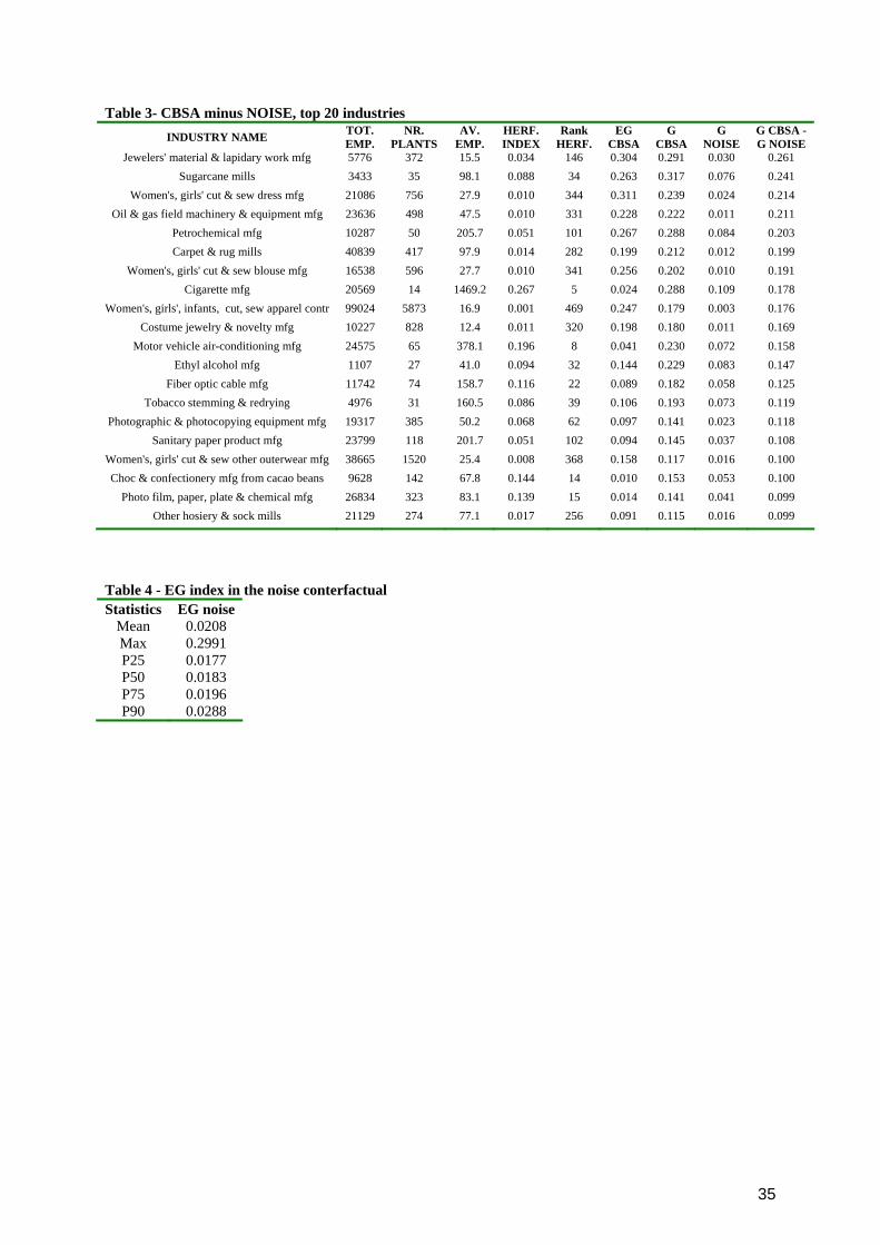
35

Table 3- CBSA minus NOISE, top 20 industries INDUSTRY NAME TOT.

EMP. NR.

PLANTS AV.

EMP. HERF. INDEX

Rank HERF.

EG CBSA

G CBSA

G NOISE

G CBSA - G NOISE

Jewelers' material & lapidary work mfg 5776 372 15.5 0.034 146 0.304 0.291 0.030 0.261 Sugarcane mills 3433 35 98.1 0.088 34 0.263 0.317 0.076 0.241

Women's, girls' cut & sew dress mfg 21086 756 27.9 0.010 344 0.311 0.239 0.024 0.214 Oil & gas field machinery & equipment mfg 23636 498 47.5 0.010 331 0.228 0.222 0.011 0.211

Petrochemical mfg 10287 50 205.7 0.051 101 0.267 0.288 0.084 0.203 Carpet & rug mills 40839 417 97.9 0.014 282 0.199 0.212 0.012 0.199

Women's, girls' cut & sew blouse mfg 16538 596 27.7 0.010 341 0.256 0.202 0.010 0.191 Cigarette mfg 20569 14 1469.2 0.267 5 0.024 0.288 0.109 0.178

Women's, girls', infants, cut, sew apparel contr 99024 5873 16.9 0.001 469 0.247 0.179 0.003 0.176 Costume jewelry & novelty mfg 10227 828 12.4 0.011 320 0.198 0.180 0.011 0.169

Motor vehicle air-conditioning mfg 24575 65 378.1 0.196 8 0.041 0.230 0.072 0.158 Ethyl alcohol mfg 1107 27 41.0 0.094 32 0.144 0.229 0.083 0.147

Fiber optic cable mfg 11742 74 158.7 0.116 22 0.089 0.182 0.058 0.125 Tobacco stemming & redrying 4976 31 160.5 0.086 39 0.106 0.193 0.073 0.119

Photographic & photocopying equipment mfg 19317 385 50.2 0.068 62 0.097 0.141 0.023 0.118 Sanitary paper product mfg 23799 118 201.7 0.051 102 0.094 0.145 0.037 0.108

Women's, girls' cut & sew other outerwear mfg 38665 1520 25.4 0.008 368 0.158 0.117 0.016 0.100 Choc & confectionery mfg from cacao beans 9628 142 67.8 0.144 14 0.010 0.153 0.053 0.100

Photo film, paper, plate & chemical mfg 26834 323 83.1 0.139 15 0.014 0.141 0.041 0.099 Other hosiery & sock mills 21129 274 77.1 0.017 256 0.091 0.115 0.016 0.099

Table 4 - EG index in the noise conterfactual Statistics EG noise

Mean 0.0208 Max 0.2991 P25 0.0177 P50 0.0183 P75 0.0196 P90 0.0288

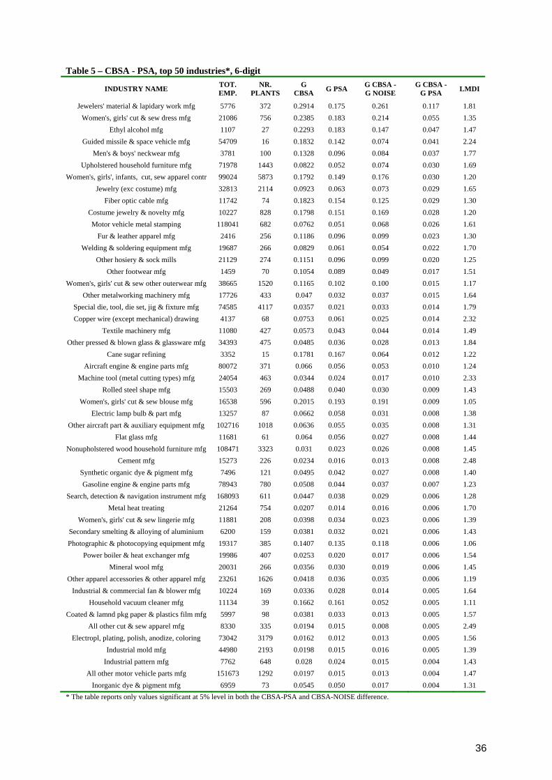
36

Table 5 – CBSA - PSA, top 50 industries*, 6-digit

INDUSTRY NAME TOT. EMP.

NR. PLANTS

G CBSA G PSA G CBSA -

G NOISE G CBSA -

G PSA LMDI

Jewelers' material & lapidary work mfg 5776 372 0.2914 0.175 0.261 0.117 1.81 Women's, girls' cut & sew dress mfg 21086 756 0.2385 0.183 0.214 0.055 1.35

Ethyl alcohol mfg 1107 27 0.2293 0.183 0.147 0.047 1.47 Guided missile & space vehicle mfg 54709 16 0.1832 0.142 0.074 0.041 2.24

Men's & boys' neckwear mfg 3781 100 0.1328 0.096 0.084 0.037 1.77 Upholstered household furniture mfg 71978 1443 0.0822 0.052 0.074 0.030 1.69

Women's, girls', infants, cut, sew apparel contr 99024 5873 0.1792 0.149 0.176 0.030 1.20 Jewelry (exc costume) mfg 32813 2114 0.0923 0.063 0.073 0.029 1.65

Fiber optic cable mfg 11742 74 0.1823 0.154 0.125 0.029 1.30 Costume jewelry & novelty mfg 10227 828 0.1798 0.151 0.169 0.028 1.20 Motor vehicle metal stamping 118041 682 0.0762 0.051 0.068 0.026 1.61

Fur & leather apparel mfg 2416 256 0.1186 0.096 0.099 0.023 1.30 Welding & soldering equipment mfg 19687 266 0.0829 0.061 0.054 0.022 1.70

Other hosiery & sock mills 21129 274 0.1151 0.096 0.099 0.020 1.25 Other footwear mfg 1459 70 0.1054 0.089 0.049 0.017 1.51

Women's, girls' cut & sew other outerwear mfg 38665 1520 0.1165 0.102 0.100 0.015 1.17 Other metalworking machinery mfg 17726 433 0.047 0.032 0.037 0.015 1.64

Special die, tool, die set, jig & fixture mfg 74585 4117 0.0357 0.021 0.033 0.014 1.79 Copper wire (except mechanical) drawing 4137 68 0.0753 0.061 0.025 0.014 2.32

Textile machinery mfg 11080 427 0.0573 0.043 0.044 0.014 1.49 Other pressed & blown glass & glassware mfg 34393 475 0.0485 0.036 0.028 0.013 1.84

Cane sugar refining 3352 15 0.1781 0.167 0.064 0.012 1.22 Aircraft engine & engine parts mfg 80072 371 0.066 0.056 0.053 0.010 1.24

Machine tool (metal cutting types) mfg 24054 463 0.0344 0.024 0.017 0.010 2.33 Rolled steel shape mfg 15503 269 0.0488 0.040 0.030 0.009 1.43

Women's, girls' cut & sew blouse mfg 16538 596 0.2015 0.193 0.191 0.009 1.05 Electric lamp bulb & part mfg 13257 87 0.0662 0.058 0.031 0.008 1.38

Other aircraft part & auxiliary equipment mfg 102716 1018 0.0636 0.055 0.035 0.008 1.31 Flat glass mfg 11681 61 0.064 0.056 0.027 0.008 1.44

Nonupholstered wood household furniture mfg 108471 3323 0.031 0.023 0.026 0.008 1.45 Cement mfg 15273 226 0.0234 0.016 0.013 0.008 2.48

Synthetic organic dye & pigment mfg 7496 121 0.0495 0.042 0.027 0.008 1.40 Gasoline engine & engine parts mfg 78943 780 0.0508 0.044 0.037 0.007 1.23

Search, detection & navigation instrument mfg 168093 611 0.0447 0.038 0.029 0.006 1.28 Metal heat treating 21264 754 0.0207 0.014 0.016 0.006 1.70

Women's, girls' cut & sew lingerie mfg 11881 208 0.0398 0.034 0.023 0.006 1.39 Secondary smelting & alloying of aluminium 6200 159 0.0381 0.032 0.021 0.006 1.43 Photographic & photocopying equipment mfg 19317 385 0.1407 0.135 0.118 0.006 1.06

Power boiler & heat exchanger mfg 19986 407 0.0253 0.020 0.017 0.006 1.54 Mineral wool mfg 20031 266 0.0356 0.030 0.019 0.006 1.45

Other apparel accessories & other apparel mfg 23261 1626 0.0418 0.036 0.035 0.006 1.19 Industrial & commercial fan & blower mfg 10224 169 0.0336 0.028 0.014 0.005 1.64

Household vacuum cleaner mfg 11134 39 0.1662 0.161 0.052 0.005 1.11 Coated & lamnd pkg paper & plastics film mfg 5997 98 0.0381 0.033 0.013 0.005 1.57

All other cut & sew apparel mfg 8330 335 0.0194 0.015 0.008 0.005 2.49 Electropl, plating, polish, anodize, coloring 73042 3179 0.0162 0.012 0.013 0.005 1.56

Industrial mold mfg 44980 2193 0.0198 0.015 0.016 0.005 1.39 Industrial pattern mfg 7762 648 0.028 0.024 0.015 0.004 1.43

All other motor vehicle parts mfg 151673 1292 0.0197 0.015 0.013 0.004 1.47 Inorganic dye & pigment mfg 6959 73 0.0545 0.050 0.017 0.004 1.31

* The table reports only values significant at 5% level in both the CBSA-PSA and CBSA-NOISE difference.

37

Table 6 – CBSA - PSA, 4-digit*, positive values

INDUSTRY NAME TOT. EMP.

NR. PLANTS

G CBSA G PSA G CBSA -

G NOISE G CBSA -

G PSA LMDI

Cut & sew apparel mfg 311677 11789 0.078 0.066 0.072 0.0122 1.19 Metalworking machinery mfg 218427 9260 0.022 0.015 0.020 0.0070 1.52 Aerospace product & parts mfg 412944 1691 0.041 0.035 0.032 0.0063 1.25 Motor vehicle parts mfg 740523 5104 0.025 0.019 0.023 0.0060 1.36 Apparel accessories & other apparel mfg 40112 2163 0.031 0.026 0.026 0.0051 1.28 Motor vehicle mfg 255966 378 0.037 0.032 0.019 0.0049 1.35 HH & institutional furniture & kitchen cabinet mfg 339880 12941 0.016 0.011 0.013 0.0048 1.49 Nav, measuring, medical, control instruments mfg 443652 4934 0.017 0.013 0.012 0.0041 1.57 Motor vehicle body & trailer mfg 125491 1748 0.035 0.031 0.025 0.0036 1.15 Steel product mfg from purchased steel 63958 863 0.014 0.011 0.009 0.0028 1.35 Clay product & refractory mfg 69827 1616 0.011 0.008 0.006 0.0027 1.99 Other transportation equipment mfg 38752 757 0.033 0.030 0.022 0.0027 1.12 Coating, engrave, heat treating & oth activity 150012 5917 0.010 0.007 0.009 0.0026 1.52 Glass & glass product mfg 117749 2124 0.013 0.011 0.008 0.0025 1.35 Mach shops, turn prod, screw, nut, bolt mfg 389848 24141 0.006 0.004 0.005 0.0019 1.65 Other nonmetallic mineral product mfg 68044 2286 0.009 0.007 0.006 0.0019 1.62 Cement & concrete product mfg 196681 7739 0.005 0.003 0.004 0.0017 1.75 Ag, construction & mining machinery mfg 161659 2442 0.017 0.015 0.014 0.0016 1.19 Other wood product mfg 258822 8661 0.009 0.007 0.007 0.0015 1.19 Other electrical equipment & component mfg 202114 2378 0.007 0.005 0.002 0.0015 2.12 Animal food mfg 41536 1314 0.011 0.009 0.007 0.0015 1.25 Boiler, tank & shipping container mfg 86680 1603 0.008 0.006 0.005 0.0015 1.30 Other fabricated metal product mfg 290455 6784 0.005 0.004 0.003 0.0015 1.76 Communications equipment mfg 244061 2165 0.022 0.021 0.012 0.0014 1.10 Other miscellaneous mfg 390362 17629 0.005 0.004 0.003 0.0012 1.46 Foundries 197312 2537 0.011 0.010 0.007 0.0010 1.24 Dairy product mfg 113462 1510 0.007 0.006 0.004 0.0010 1.36 Rubber product mfg 190260 2479 0.010 0.009 0.007 0.0006 1.21 Other general purpose machinery mfg 307881 6209 0.005 0.004 0.003 0.0005 1.38 Plastics product mfg 763061 12501 0.003 0.003 0.002 0.0004 1.37

Architectural & structural metals mfg 369395 10911 0.002 0.002 0.001 -0.0002 0.97 * The table reports only values significant at 5% level in both the CBSA-PSA and CBSA-NOISE difference.