Modelling the Ghanaian Inflation Rates Using Interrupted ...

Mathematical Theory and Modeling www.iiste.org

ISSN 2224-5804 (Paper) ISSN 2225-0522 (Online)

Vol.6, No.2, 2016

97

Modelling the Ghanaian Inflation Rates Using Interrupted Time

Series Analysis Approach

Hudu Mohammed1, Abdul-Aziz A.R.

2, Bashiru I. I. Saeed (PhD)

3

Lecturer, Mathematics and Statistics Department, Kumasi Polytechnic, Kumasi, Ghana

Senior Lecturer, Mathematics and Statistics Department, Kumasi Polytechnic, Kumasi, Ghana

Senior Lecturer, Mathematics and Statistics Department, Kumasi Polytechnic, Kumasi, Ghana

Abstract

The article considers the application of interrupted time series analysis to model yearly inflation rates in Ghana

from 1996 to 2006. This article, therefore, explored the effectiveness of the economic policy intervention in the

year 2001 on the inflation rate time series for the period 2001 to 2006 using the interrupted time series

experiment. We also sort to use this model to make forecasts of future values. To achieve this objective, yearly

inflation rates for the period were obtained from Bank of Ghana (BoG). The Box-Jenkins Autoregressive

Integrated Moving Average (ARIMA) method with interruption was employed in analyzing the data using

Statistical Product for Service Solution (SPSS) version 20. It was found that the rate of inflation in Ghana can be

fitted with an autoregressive model of order one, i.e. AR (1) model. From the results of the tests of the

difference between the means before and after intervention, as well as the interrupted time series experiment,

indicated that the intervention successfully reduced the rate of inflation in the Ghana’s economy.

Keywords: Inflation, Interrupted Time Series, Box-Jenkins Method.

1. Introduction

In Ghana, the debate of achieving a single digit inflation value has been the major concern for both the government

and the opposition parties. While the government boasts of a stable economy with consistent single digit

inflation, the opposition parties’ doubts these figures and believe that the figures had been cooked up and do not

reflect the true situation in the economy. Webster (2000) defined inflation as the persistent increase in the level

of consumer prices or a persistent decline in the purchasing power of money. Price stability (stable inflation) is

one of the main objectives of every government as it is an important economic indicator that the government,

politicians, economists and other stakeholders use as their basis of argument when debating on the state of the

economy (Suleman and Sarpong, 2012). In recent years, rising inflation has become one of the major economic

challenges facing most countries in the world especially developing countries like Ghana. David (2001) described

inflation as a major focus of economic policy worldwide.

Inflation and its volatility entail large real costs to the economy (Moreno, 2004). Among the harmful effects

of inflation volatility are the higher risk of permia for long term arrangement, unforeseen redistribution of

wealth and higher costs for hedging against inflation risks (Rother, 2004). Thus inflation volatility

canimpede growth even if inflation on the average remains restrained (Awogbemi and Oluwaseyi, 2011)

and hence monetary policy makers are more interested in containing and reducing inflation through price

stability (Amos, 2010). Policy makers will be content and satisfied if they are able to understand the

underlying dynamics of inflation and how it evolves. Ngailo (2011) observes that inflation dynamics and

evolution can be studied using a stochastic modelling approach that captures the time dependent

structure embedded in the time series inflation data.

Inflation is a persistent rise in the general price levels of goods and services in an economy over a period of

time. Inflation rate has been regarded as one of the main economic indicators in any country. According to

Olatunji et al. (2010), inflation undoubtedly remains as one of the leading and most dynamic macro-economic

issues confronting almost all economies of the world. Its dynamism has made it an imperative issue to be

considered. Odusanya and Atanda (2010) determined the dynamic and simultaneous interrelationship between

inflation and its determinants – growth rate of Gross Domestic Product (GDP), growth rate of money supply

(M2), fiscal deficit, exchange rate (U.S dollar to Naira), importance and interest rates, using econometric time

http://www.iiste.org/



Vol.6, No.2, 2016

98

series model. Olatunji et al. (2010) examined the factors affecting inflation in Nigeria using cointegration and

descriptive statistics. They observed that there were variations in the trend pattern of inflation rates and some

variables considered were significant in determining inflation in Nigeria. These variables include annual total

import, annual consumer price index for food, annual agricultural output, interest rate, annual government

expenditure, exchange rate and annual crude oil export.

Some econometric models have been used to describe inflation rates, but they are restrictive in their theoretical

formulations and often do not incorporate the dynamic structure of the data and have tendencies to inflict

improper restrictions and specifications on the structural variables (Saz, 2011). Mordi et al. (2007), in their

study of the best models to use in forecasting inflation rates in Nigeria identified areas of future research on

inflation dynamics to include re-identifying ARIMA models, specifying and estimating VAR models and

estimating a P-Star model, amongst others that can be used to forecast inflation with minimum mean square

error.

The absence of restriction in the ARIMA model gives it the necessary flexibility to capture dynamic properties

and thus significant advantage in short-run forecasting (Saz, 2011). Encouraged by these empirical results on the

superiority of ARIMA models, Saz (2011) applied Seasonal Autoregressive Integrated Moving Average

(SARIMA) model to forecast the Turkish inflation. Longinus (2004) examined the influence of the major

determinants of inflation with a particular focus on the role of exchange rate policy of Tanzania from 1986 to

2002. He discovered that the parallel exchange rate had a stronger influence on inflation. Other works on

modeling inflation rates are seen in the works of Fatukasi (2003), Eugen et al. (2007) and Tidiane (2011).

This paper explores the effectiveness of the economic policy intervention in the year 2001 on the inflation rate

time series for the period 2001 to 2006 using the interrupted time series experiment. We also seek to use this

model to make forecasts of future values.

2.0 Materials and Method

2.1 Model Specification

2.1.1 ARMA or “Mixed” Process

Consider the process given by;

𝑌𝑡 = 𝛼1𝑌𝑡−1 + 𝜃1𝑒𝑡−1 + 𝑒1

This can be rewritten as

𝑌𝑡 − 𝛼1𝑌𝑡−1 = 𝑒𝑡 + 𝜃1𝑒𝑡−1 Or

(1 − 𝛼𝐵)𝑌𝑡 = (1 + 𝜃𝐵)𝑒𝑡…………………………….. (1)

𝐴𝑅(𝐵)𝑌𝑡 = 𝑀𝐴(𝐵)𝑒𝑡

This is called a mixed or autoregressive moving average (ARMA) process of order (1,1).

Since equation (1) is ARMA(1,1) if |𝜃| < 1 it can be rewritten as

(1 − 𝛼𝐵) (1

1 + 𝜃𝐵) 𝑌𝑡 = 𝑒𝑡

(1 − 𝛼𝐵)(1 − 𝜃𝐵 + 𝜃2𝐵2 − 𝜃3𝐵3 + ⋯ )𝑌𝑡 = 𝑒𝑡

[(1 − 𝛼 + 𝜃)𝐵 + (𝛼𝜃 + 𝜃2)𝐵2 + ⋯ ]𝑌𝑡 = 𝑒𝑡

This is an infinite order AR process. This is true if |𝛼| < 1 and |𝜃| < 1 i.e. if the AR is stationary and MA is

invertible. If we have two polynomial in B, MA(B) and AR(B), and an ARMA model,

𝐴𝑅(𝐵)𝑌𝑡 = 𝑀𝐴(𝐵)𝑒𝑡




Vol.6, No.2, 2016

99

It is possible to write the model as an infinite AR process:

(𝐴𝑅(𝐵)

𝑀𝐴(𝐵)) 𝑌𝑡 = 𝑒𝑡

Or an infinite MA process

𝑌𝑡 = (𝑀𝐴(𝐵)

𝐴𝑅(𝐵)) 𝑒𝑡

And approximate either by finite processes

ARMA processes are parsimonious however identifying those using ACF and PACF may be difficult. The

condition necessary for dividing by AR(B) is that the AR process be stationary and by MA(B) is that the MA

process be invertible.

2.1.2 Autoregressive Moving Average Model (ARMA)

A more general model is a mixture of the AR(p) and MA(q) models and is called an autoregressive moving

average model (ARMA) of order (p,q).

The ARMA(p,q) is given by

𝑌𝑡 = ∑ 𝛼𝑖𝑌𝑖−1𝑝𝑖=1 + ∑ 𝜃𝑖𝑒𝑖−1

𝑞𝑖=1 + 𝜇 + 𝑒𝑡

An example of an ARMA(1,1)

𝑌𝑡 = 𝛼1𝑌𝑡−1 + 𝜃1𝑒𝑡−1 + 𝜇 + 𝑒𝑡

An important characteristic of ARMA models is that both the ACF and PACF do not cut off as in AR and MA

models.

(Box and Jenkins, 1971)

2.1.3 The Autoregressive Integrated Moving Average Model (ARIMA)

If a non-stationary time series which has variation in the mean is differenced to remove the variation the

resulting time series is called an integrated time series. It is called an integrated model because the stationary

model which is fitted to the differenced data has to be summed or integrated to provide a model for the non-

stationary data. Notationally, all AR(p) and MA(q) models can be represented as ARIMA(1,0,0) that is no

differencing and no MA part.

The general model is ARIMA(p,d,q) where p is the order of the AR part, d is the degree of differencing and q is

the order of the MA part.

Writing 𝑊𝑡 = ∇𝑑𝑌𝑡 = (1 − 𝐵)𝑑𝑌𝑡

The general ARIMA process is of the form

𝑊𝑡 = ∑ 𝛼𝑖𝑊𝑡−𝑖𝑝𝑡=1 + ∑ 𝜃𝑖𝑒𝑡−𝑖

𝑞𝑡=1 + 𝜇 + 𝑒𝑡

(Hamilton J.D, 1994)

2.1.4 Extension of the Procedure to AR(p) Models

Assume that 𝑛1 data points before intervention consist of a stationary stochastic component, which is fitted with

an autoregressive model, plus a linear trend. Thus before intervention (𝑡 = 𝑝 + 1, 𝑝 + 2, … 𝑛1) the data can be

represented as

𝑌𝑡 = 𝑚1𝑡 + 𝑏1 + ∑ 𝛼𝑖𝑌𝑖−1

𝑝

𝑡=1

+ 𝑒𝑡




Vol.6, No.2, 2016

100

After intervention (𝑡 = 𝑛𝑡+1, … , 𝑁) and assume 𝑛2 = 𝑁 − 𝑛 data points move to a new asymptotic trend line. It

is further assumed that the autoregressive parameters have not changed as a result of the intervention. Thus after

the intervention the data can be represented as

𝑌𝑡 = 𝑚2𝑡 + 𝑏2 + ∑ 𝛼𝑖𝑌𝑡−𝑖 + 𝑒𝑡

𝑝

𝑡=1

The next stage is to estimate the parameters 𝑚1, 𝑏1, 𝛼1, 𝑚2 𝑎𝑛𝑑 𝑏2. one proceeds to find whether there has been

significant changes in the values of 𝑚1 and 𝑏1 as reflected in the values of 𝑚2 and 𝑏2 which will be used to test

whether the intervention was successful.

4

6

5

4

3

2

1

2

1

2

2

1

1

.

.

.

.

.

.

pp

m

b

m

b

N

p

p

e

e

e

E

.

.

.

.

2

1

As usual the least squares estimates are

𝛽 = (𝑋𝑇𝑋)−1𝑋𝑇𝑌

If the estimate of 𝜎𝑒2 is denoted by 𝑆𝑒

2 which (1

𝑣) (𝑌 − 𝑋𝛽)𝑇(𝑌 − 𝑋𝛽),

Where v, the degrees of freedom for errors is 𝑁 − 2𝑝 − 4 and denote the C as the diagonal of (𝑋𝑇𝑋)−1, then

each of the parameters in 𝛽𝑖 = (𝑏1, 𝑚1, 𝑏2, 𝑚2, 𝛼1, … , 𝛼𝑝) can be referred to a

𝑡-distribution with 𝑣 degrees of freedom, where

𝑇 = 𝛽1

𝑆𝑒√𝐶𝑖

The data points do not actually lie on the lines 𝑚1𝑡 + 𝑏1 before and 𝑚2𝑡 + 𝑏2 after intervention. Rather, before

intervention the data follow a steady-state trend line of the form 𝐵1 + 𝑀1𝑡 and approach 𝐵2 + 𝑀2𝑡 after

intervention.

2.3 Estimation of Parameters

2.3.1 Estimating the Parameters of an ARMA Model

The procedure for estimating the parameters of the ARMA model is like the one for the MA model it is an

iterative method. Like the MA the residual sum of squares is calculated at every point on a suitable grid of the

parameter values, and the values, and the values give the minimum sum of squares are the estimates.

For an ARMA (1, 1) the model is given by

𝑌𝑡 − 𝜇 = 𝛼1(𝑌𝑡−1 − 𝜇)𝑒𝑡 + 𝜃1𝑒𝑡−1




Vol.6, No.2, 2016

101

Given N observation 𝑌1, 𝑌2, … , 𝑌𝑁 , we guess values for 𝜇, 𝛼1, 𝜃1, set 𝑒0 = 0 and 𝑌0 = 0 and then calculate the

residuals recursively by

𝑒1 = 𝑌1 − 𝜇

𝑒2 = 𝑌2 − 𝜇−𝛼1(𝑌1 − 𝜇) − 𝜃1𝑒1

… … … … … … … … … … … ..

… … … … … … … … … … ….

𝑒𝑁 = 𝑌𝑁 − 𝜇 − 𝛼1(𝑌1 − 𝜇) − 𝜃1𝑒𝑁−1

The residual sum of squares ∑ 𝑒𝑡2𝑁

𝑡=1 is calculated. Then other values of𝜇, 𝛼1, 𝜃1, are tried until the minimum

residual of squares is found.

Note: It has been found that most of the stationary time series occurring in practices can be fitted by AR(1),

AR(2), MA(1), MA(2), ARMA(1,1) or white noise models that are customarily needed in practice.

(Hamilton J.D, 1994)

2.3.2 Estimating the parameters of an ARIMA Model

In practice most time series are non-stationary and the series is differenced until the series becomes stationary.

An AR, MA or ARMA model is fitted to the differenced series and estimation procedures are as described for

the AR, MA, ARMA above.

2.4 Tests

2.4.1 The Box-Jenkins Method of Modeling time Series

The Box-Jenkins methodology is a statistical sophisticated way of analyzing and building a forecasting model

which best represents a time series. The first stage is the identification of the appropriate ARIMA models

through the study of the autocorrelation and partial autocorrelation functions. For example if the partial

autocorrelation cuts off after lag one and the autocorrelation function decays then ARIMA(1,0,0) is identified.

The next stage is to estimates the parameters of the ARIMA model chosen.

The third stage is the diagnostic checking of the model. The Q-statistic is used for the model adequacy check.

If the model is not adequate then the forecaster goes to stage one to identify an alternative model and it is tested

for adequacy and if adequacy then the forecaster goes to the final stage of the process.

The fourth stage is where the analysis uses the model chosen to forecast and the process ends.

2.4.2 Measurement of the intervention Effect

The procedure used in this work is to fit an AR(p) an autoregressive model of order p to the interrupted time

series data using the Box-Jenkins methods of fitting a model to a time series data. The next step is to use the

least squares method to estimate the parameters and statistical methods to assess the effectiveness of the

intervention. (McDowall, et al)

Let us consider an imaginary interrupted time series data which can be fitted with a stationary AR(1) model

which has a zero mean.

𝑌𝑡 = 𝛼1𝑌𝑡−1 + 𝑒𝑡 where 𝛼1 is the AR(1) parameter and 𝑒𝑡 is the white noise. Let us assume further that we

have 𝑛1 data points before intervention and 𝑛2 points after intervention and 𝑛1 + 𝑛2 = 𝑁. Suppose we assume

that the effect is to add 𝛾 to the mean level.




Vol.6, No.2, 2016

102

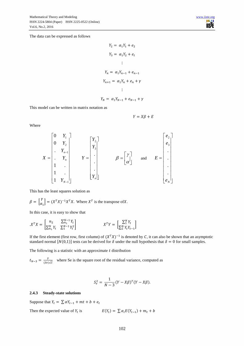
The data can be expressed as follows

𝑌2 = 𝛼1𝑌1 + 𝑒2

𝑌3 = 𝛼1𝑌2 + 𝑒𝑡

⋮

𝑌𝑛 = 𝛼1𝑌𝑛−1 + 𝑒𝑛−1

𝑌𝑛+1 = 𝛼1𝑌𝑛 + 𝑒𝑛 + 𝛾

⋮

𝑌𝑁 = 𝛼1𝑌𝑁−1 + 𝑒𝑁−1 + 𝛾

This model can be written in matrix notation as

𝑌 = 𝑋𝛽 + 𝐸

Where

1

1

2

1

1

.1

.1

.

.

0

0

N

n

n

Y

Y

Y

Y

Y

X

nY

Y

Y

Y

.

.

.

3

2

and

Ne

e

e

E

.

.

.

.

3

2

This has the least squares solution as

𝛽 = [𝛾

𝛼1] = (𝑋𝑇𝑋)−1𝑋𝑇𝑋. Where 𝑋𝑇 is the transpose of𝑋.

In this case, it is easy to show that

.𝑋𝑇𝑋 = [𝑛2 ∑ 𝑌𝑡

𝑁−1𝑛1

∑ 𝑌𝑡𝑁𝑛1

∑ 𝑌𝑡2𝑁−1

1

] 𝑋𝑇𝑌 = [∑ 𝑌𝑡

𝑁1

∑ 𝑌𝑡𝑌𝑡−1𝑁2

]

If the first element (first row, first column) of (𝑋𝑇𝑋)−1 is denoted by 𝐶, it can also be shown that an asymptotic

standard normal [𝑁(0,1)] tests can be derived for 𝛿 under the null hypothesis that 𝛿 = 0 for small samples.

The following is a statistic with an approximate 𝑡 distribution

𝑡𝑁−3 = 𝛾

(𝑆𝑒)√𝑐 where Se is the square root of the residual variance, computed as

𝑆𝑒2 =

1

𝑁 − 3(𝑌 − 𝑋𝛽)𝑇(𝑌 − 𝑋𝛽).

2.4.3 Steady-state solutions

Suppose that 𝑌𝑡 = ∑ 𝛼𝑌𝑡−1 + 𝑚𝑡 + 𝑏 + 𝑒𝑡

Then the expected value of 𝑌𝑡 is 𝐸(𝑌𝑡) = ∑ 𝛼𝑖𝐸(𝑌𝑡−1) + 𝑚𝑡 + 𝑏




Vol.6, No.2, 2016

103

To find the steady-state solution of this difference equation in 𝐸(𝑌𝑡), we assume

𝑀𝑡 + 𝐵 = ∑ 𝛼𝑖 (𝑀(𝑡 − 1) + 𝐵) + 𝑚𝑡 + 𝑏

Equating coefficients of t and constant terms we have

𝑀𝑡 = (∑ 𝛼𝑖) 𝑀𝑡 + 𝑚𝑡

𝐵 = ∑ 𝛼𝑖(−𝑖)𝑀 + (∑ 𝛼𝑖) + 𝑚𝑡 + 𝑏

So that 𝑀 = 𝑚

1−∑ 𝛼𝑖 and 𝐵 =

𝑏−𝑀(∑ 𝛼𝑖)

1−∑ 𝛼𝑖

For example for an AR(p) model with n1 data points before intervention and n2 data points after intervention

where n1 + n2 = N, the model becomes

𝑌𝑡 = 𝑚1𝑡 + 𝑏1 + ∑ 𝛼𝑖𝑌𝑡−1 + 𝑒𝑡

𝑝

𝑖=1

Before intervention and

𝑌𝑡 = 𝑚2𝑡 + 𝑏2 + ∑ 𝛼𝑖𝑌𝑡−1 + 𝑒𝑡

𝑝

𝑡=1

After intervention.

The matrix notation is follows

N

N

Y

Y

Y

Y

Y

.

.

21

4

3

212

1

111

2111

23

12

100

......

......

.2200

1100

0010

......

......

0021

0011

NN

n

NN

nN

YYn

Y

YY

YYN

YY

YY

X

1

2

2

1

1

B

M

B

M

6

5

4

3

2

1

Ne

e

e

E

.

.

.

4

3




Vol.6, No.2, 2016

104

And 𝛽 = (𝑋𝑇𝑋)−1 𝑋𝑇𝑋 and 𝑇 = 𝛽1

𝑆𝑒√𝐶𝑖 𝑖 = 1, 2, 3, 4

2.4.4 Testing for the significance of the Intervention

Here we test:

𝐻0 ∶ 𝑚1 = 𝑚2, 𝑏1 = 𝑏2 (𝑖𝑛𝑡𝑒𝑟𝑣𝑒𝑛𝑡𝑖𝑜𝑛 𝑖𝑛𝑒𝑓𝑓𝑒𝑐𝑡𝑖𝑣𝑒 )

Against:

𝐻1 ∶ 𝑚1 ≠ 𝑚2, 𝑏1 ≠ 𝑏2 (𝑖𝑛𝑡𝑒𝑟𝑣𝑒𝑛𝑡𝑖𝑜𝑛 𝑒𝑓𝑓𝑓𝑒𝑐𝑡𝑖𝑣𝑒)

Let 𝑆𝑆0 denote the residual error sum of squares in the reduced model.

𝑌𝑡 = 𝑚1 + 𝑏 + ∑ 𝛼𝑖𝑌𝑖−1 + 𝑒𝑡 𝑓𝑜𝑟 𝑎𝑙𝑙 𝑡

𝑝

𝑖=1

And let 𝑆𝑆0 denote the residual sum of squares in the full model

𝑌𝑡 = 𝑚1𝑡 + 𝑏1 + ∑ 𝛼𝑖𝑌𝑖−1 + 𝑒𝑡 𝑡 = 𝑝 + 1, . . . , 𝑛1

𝑝

𝑖=1

And

𝑌𝑡 = 𝑚2𝑡 + 𝑏2 + ∑ 𝛼𝑖𝑌𝑖−1 + 𝑒𝑡 𝑡 = 𝑛1, … , 𝑁

𝑝

𝑖=1

Then under the null hypothesis,

𝐹 =

(𝑆𝑆0 − 𝑆𝑆1)2⁄

𝑆𝑆1𝑣⁄

Has an F(1,v) distribution. Here 𝑣, the error degrees of freedom is equal to the number of observations minus

the number of “start up” observations (2 in AR(2) model or 3 in AR(3) minus the number of parameters fit, that

is 6 in AR(2) and 4 in AR(1).

3.0 Results

3.1 Identification of the Model

The autocorrelation function dies down and the partial autocorrelation function cuts off after lag one. This

identifies an AR (1) process which has the form

𝑌𝑡 = 𝛼𝑌𝑡−1 + 𝑒𝑡

Fig. 1 and Fig. 2 shows the graph of the autocorrelation and partial autocorrelation functions respectively.




Vol.6, No.2, 2016

105

Fig 1 ACF of monthly inflation rate in Ghana from Jan. 96 to Dec. 06

Fig 2 PACF of monthly inflation rate in Ghana from Jan. 96 to Dec. 06

Table 1 Analysis of the time series data

ARIMA MODEL RESIDUAL

VARIANCE

AIC Q-VALUE

(1,0,0) 6.197 566.019 16.780

Since the interrupted time series analysis look out for an ARIMA (p.0.0), the ARIMA (1,0,0) is the best model

for the time series data and it is also adequate since the Q- value is less than the critical value. It has the form

𝑌𝑡 = 0.995𝑌𝑡−1 + 37.657

242322212019181716151413121110987654321

Lag Number

1.0

0.5

0.0

-0.5

-1.0

ACF

Lower ConfidenceLimit

Upper Confidence Limit

Coefficient

Rates

242322212019181716151413121110987654321

Lag Number

1.0

0.5

0.0

-0.5

-1.0

Parti

al A

CF

Lower ConfidenceLimit

Upper Confidence Limit

Coefficient

Rates




Vol.6, No.2, 2016

106

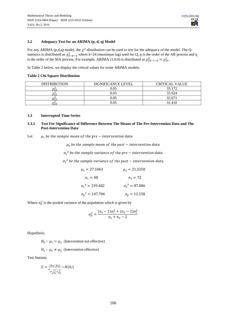
3.2 Adequacy Test for an ARIMA (p, d, q) Model

For any ARIMA (p,d,q) model, the 𝜒2-distribution can be used to test for the adequacy of the model. The Q-

statistics is distributed as 𝜒𝑘−𝑝−𝑞2 where k=24 (maximum lag) used for Q, p is the order of the AR process and q

is the order of the MA process. For example, ARIMA (1,0,0) is distributed as 𝜒24−1−02 = 𝜒23

2 .

In Table 2 below, we display the critical values for some ARIMA models.

Table 2 Chi Square Distribution

DISTRIBUTION SIGNIFICANCE LEVEL CRITICAL VALUE

𝜒232 0.05 35.172

𝜒222 0.05 33.924

𝜒212 0.05 32.671

𝜒202 0.05 31.410

3.3 Interrupted Time Series

3.3.1 Test For Significance of Difference Between The Means of The Pre-Intervention Data and The

Post-Intervention Data

Let 𝜇1 𝑏𝑒 𝑡ℎ𝑒 𝑠𝑎𝑚𝑝𝑙𝑒 𝑚𝑒𝑎𝑛 𝑜𝑓 𝑡ℎ𝑒 𝑝𝑟𝑒 − 𝑖𝑛𝑡𝑒𝑟𝑣𝑒𝑛𝑡𝑖𝑜𝑛 𝑑𝑎𝑡𝑎

𝜇2 𝑏𝑒 𝑡ℎ𝑒 𝑠𝑎𝑚𝑝𝑙𝑒 𝑚𝑒𝑎𝑛 𝑜𝑓 𝑡ℎ𝑒 𝑝𝑜𝑠𝑡 − 𝑖𝑛𝑡𝑒𝑟𝑣𝑒𝑛𝑡𝑖𝑜𝑛 𝑑𝑎𝑡𝑎

𝜎12 𝑏𝑒 𝑡ℎ𝑒 𝑠𝑎𝑚𝑝𝑙𝑒 𝑣𝑎𝑟𝑖𝑎𝑛𝑐𝑒 𝑜𝑓 𝑡ℎ𝑒 𝑝𝑟𝑒 − 𝑖𝑛𝑡𝑒𝑟𝑣𝑒𝑛𝑡𝑖𝑜𝑛 𝑑𝑎𝑡𝑎

𝜎22 𝑏𝑒 𝑡ℎ𝑒 𝑠𝑎𝑚𝑝𝑙𝑒 𝑣𝑎𝑟𝑖𝑎𝑛𝑐𝑒 𝑜𝑓 𝑡ℎ𝑒 𝑝𝑜𝑠𝑡 − 𝑖𝑛𝑡𝑒𝑟𝑣𝑒𝑛𝑡𝑖𝑜𝑛 𝑑𝑎𝑡𝑎

𝜇1 = 27.1063 𝜇2 = 21.3250

𝑛1 = 48 𝑛2 = 72

𝜎12 = 239.482 𝜎2

2 = 87.086

𝜎𝑝2 = 147.786 𝜎𝑝 = 12.158

Where 𝜎𝑝2 is the pooled variance of the population which is given by

𝜎𝑝2 =

(𝑛1 − 1)𝜎12 + (𝑛2 − 1)𝜎2

2

𝑛1 + 𝑛2 − 2

Hypothesis

𝐻0 ∶ 𝜇1 = 𝜇2 (Intervention not effective)

𝐻1 ∶ 𝜇1 ≠ 𝜇2 (Intervention effective)

Test Statistic

𝑍 =(𝜇1−𝜇2)

𝜎𝑃√

1𝑛1

+1

𝑛2

~𝑁(0,1




Vol.6, No.2, 2016

107

Decision Rule

𝐼𝑓 𝑍 ≥ 1.65, 𝑟𝑒𝑗𝑒𝑐𝑡 𝐻0 𝑎𝑛𝑑 𝑎𝑐𝑐𝑒𝑝𝑡 𝐻1

𝐼𝑓 𝑍 < 1.65, 𝑎𝑐𝑐𝑒𝑝𝑡 𝐻0 𝑎𝑛𝑑 𝑟𝑒𝑗𝑒𝑐𝑡 𝐻1

Calculation

𝑍 =(27.1063 − 21.3250)

12.158√ 148

+1

72

= 2.552

Since Z=2.552 > 1.65 we reject H0 and accept H1 and conclude that there is enough evidence at the 5% level of

significance of a decrease in the mean level of the inflation in Ghana after the intervention policy in 2000.

3.3.2 USE OF REGRESSION ANALYSIS TO MODEL TREND AND AUTOREGRESSIVE

COMPONENTS

We attempt to apply the interrupted time series analysis described in section 2.0 to estimates b1, b2, m1, m2, 𝛼.

Here b1 and b2 are the intercepts and m1 and m2 are the slopes before and after intervention while 𝛼 is the AR

parameters. This is done by use of SPSS for the regression analysis.

The results for the full and reduced models are displayed in the tables below.

Table 3 Variables in the equation of full model

VARIABLE ESTIMATES STD.

ERROR

95% CI

LOWER

95%CI

UPPER

T-VALUE SIG.

B1 1.230 1.529 -1.800 4.260 0.804 0.423

M1 -.004 0.035 -0.074 0.066 -0.117 0.907

B2 3.097 0.961 1.193 5.001 3.222 0.002

M2 -.036 0.014 -0.064 -0.008 -2.532 0.013

𝛼 .916 0.027 0.000 0.970 34.002 0.000

Table 4 Model efficiency of full model

R R-SQUARE ADJUSTED R STD. ERROR

0.997 0.993 0.993 2.19774

From the Table 4 it indicates that about 99.3% of the variability in the inflation was explained by the predictor

variables with standard error of about 2.19774.

Table 5 ANOVA of full model

MODEL DF SSS MSE F SIG. F

REGRESSION 5 80110.663 16022.133 3317.167 0.000

RESIDUAL 114 550.627 4.830




Vol.6, No.2, 2016

108

From Table 5 above, the value of the p-value is less than the significance level (0.05). This means that there is

sufficient evidence to reject the null hypothesis and conclude that the intervention effect was effective at 95%

confidence level.

The autocorrelation function dies down and the partial autocorrelation function cuts off after lag one

indicating an autoregressive process of order one i.e. AR (1) process. The model is;

Yt = 0.995Yt-1 + 37.657

The significance test of the difference between the means of the pre and post intervention data was significant.

There was enough evidence at the 5% level of significance that the mean before the intervention was greater

than the mean after the intervention.

4. Conclusion

It was found that the rate of inflation in Ghana can be fitted with an autoregressive model of order one, i.e. AR

(1) model. From the results of the tests of the difference between the means before and after intervention, as

well as the interrupted time series experiment, it means/imply that the intervention has successfully reduced the

rate of inflation in the nation.

It is recommended that the Government continues with the tight monetary policy, Open Market Operations

(OMO), Repurchase Agreements (Repos) and prime rate (interest Rate) policies that has been used since Jan

2000 to Dec 2006 in trying to reduce the rate of inflation since it was effective.

Also further study that relates interest rate to inflation could be carried researched into.

References

1. Dodge, E.R. (2011): Expansionary and Contractionary Fiscal Policy Review for AP Economics. Available

at www.education.com/study-help/article/expansionary-contractionary-fiscal-policy

2. Eugen F. and Cyprian, S. (2007): A multiple Regression model for Inflation rates in Romania In the

enlarged EU. Available Online at: http://mpra.ub.uni-muenchen.de/11473/

3. Fatukasi B. (2003): Determinants of Inflation in Nigeria: An Empirical Analysis. International Journal of

Humanities and Social Science, 1(18). Available Online at: www.ijhssnet.com

4. Gary G. M. (1995): The Main Determinants of Inflation in Nigeria. IMF Staff Papers.International

Monetary Fund, 42(2), 270-289.

5. Longinus R. (2004): Exchange rates Regimes and Inflation in Tanzania.AERC Research Paper 38, African

Economic Research Consortium, Nairobi.

6. Mordi, C.N.O, Essien, E.A, Adenuga, A.O, Omanukwe, P.N, Ononugbo, M.C, Oguntade, A.A, Abeng,

M.O, Ajao, O.M (2007): The Dynamics of Inflationin Nigeria: Main Report. Occasional Paper No. 2.

Research and Statistics Department. Central Bank of Nigeria, Abuja.

7. Odusanya, I. A., and Atanda, A. A. M (2010): Analysis of Inflation and its Determinants in Nigeria:

Pakistan Journal of Social Sciences 7(2): 97-100.

8. Olatunji, G. B, Omotesho, O. A, Ayinde, O. E, and Ayinde, K (2010): Determinants of Inflation in Nigeria:

A Co-integration Approach. Joint 3rd Africa Association of Agricultural Economists (AAAE) and 48th

Agricultural Economists Association of South Africa (AEASA) Conference, Cape Town, South Africa,

September 19-23.

9. Tidiane, K. (2011): Modeling Inflation in Chad. IMF Working Paper. International Monetary Fund.

10. Suleman, N., & Sarpong, S. (2012). Empirical Approach to Modelling and Forecasting

Inflation in Ghana. Current Research Journal of Economic Theory 4, (3), 83-87.

11. David, F. H. (2001). Modelling UK Inflation, 1875-1991. Journal of Applied Econometrics, 16(3):

255-275.




Vol.6, No.2, 2016

109

12. Webster, D. (2000). Webster's New Universal Unabridged Dictionary. Barnes &

Noble Books, New York

13. Moreno, A. (2004). Reaching Inflation Stability. Departmato de Economia, Universidad de Navara,

Spain.

14. Rother, P. C. (2004). Fiscal Policy and Inflation Volatility. European Central Bank Working Paper Series,

317.

15. Amos, C. (2010). Time Series Modelling with Applications to South African Inflation

Data (Unpublished master’s thesis). University of Kwazulu Natal.

16. Ngailo, E. (2011). Modelling and Forecasting using time series GARCH models: An Application of

Tanzania inflation rate data. (Unpublished Master’s Thesis). University of Dares Salaam.

17. Hamilton, J.D. (1994). TIME SERIES ANALYSIS, Princeton University Press.


Modelling the Ghanaian Inflation Rates Using Interrupted ...

Documents

Transcript of Modelling the Ghanaian Inflation Rates Using Interrupted ...