Does government spending crowd in private consumption? Theory ...

MODELLING REAL PRIVATE CONSUMPTION
EXPENDITURE - AN EMPIRICAL STUDY ON FIJI
Bimal Singh
Working Paper
2004/05
December 2004
Economics Department
Reserve Bank of Fiji
Suva
Fiji
The views expressed herein are those of the author and do not necessarily reflect those of the Reserve Bank of Fiji. The author is grateful to Mr Filimone Waqabaca and colleagues of the Economics Department of the Reserve Bank of Fiji for comments and suggestions on earlier drafts.

Abstract
This paper presents a model for Fiji’s real private consumption
expenditure, with the aim of generating a better understanding of the factors
that determine private consumption in Fiji and for the purpose of
forecasting consumption expenditure growth. The model is estimated over
the period 1979 to 2001 as an error correction model (ECM), allowing for
lagged terms so as to capture dynamic adjustment effects. The results
suggest that Fiji’s real private consumption adjusts fast to equilibrium
levels in the current period (t), from a disequilibrium experienced in the
previous period (t-1). In the short run, real private consumption growth is
significantly affected by changes in income, wealth, the real interest rate
and net private transfers. The long run (steady state) model estimates the
relationship between consumption, wealth and income. Both the wealth
variable and income were significant in determining long run consumption
growth. Moreover, results of the forecast evaluation indicate that the
parsimonious short run model has the potential to provide reliable
consumption forecasts in the medium term.

2
1.0 Introduction
Private consumption expenditure is the largest component of total
spending in Fiji, and accounts for around two-thirds of the nation’s Gross
Domestic Products (GDP). Private Consumption between 1979 and 2001
has averaged around 65 percent of GDP annually. This makes private
consumption in Fiji an extremely important component of aggregate
demand, not only because it influences economic growth, but also in the
determination of the economic cycle. In this respect, the study of
consumption is relevant.
The consumption function has featured in macro-models since
Keynes (1936), followed by Modigliani and Brumburg (1954), Friedman
(1957), Hall (1978), and the influential consumption model of David,
Hendry, Srba and Yeo (1978). Theories and empirical evidence of these
studies have formed the foundation for many later studies in consumption
behaviour.
In this paper, an econometric consumption model for Fiji is
constructed. The Error Correction Model (ECM) approach is employed
and time series data is used in the regression. The primary purpose of this
study is to generate a better understanding of the factors determining
private consumption in Fiji and to estimate a consumption function to be
used for medium term forecasting.
Consumption is expressed as a function of explanatory
variables such as income, wealth and those that capture income
uncertainty and intertemporal substitution effects. Such studies
have been common in developed countries, but are limited in small

3
developing countries such as Fiji, due to unavailability of data on all key
variables. Omission of these variables from a consumption model implies
that consumption in the model is miss-specified thus raising the familiar
econometric problems of spurious regression and omitted variable or
measurement errors. The rest of the paper is structured as follows: Section
2 briefly reviews literature. Section 3 provides a commentary on the trends
in real private consumption growth for the sample period 1979 to 2001.
The subsequent section sets out the consumption model, while Section 5
discusses the methodology. Section 6 presents the empirical results and the
final section concludes the paper.
2.0 Literature Review
There is a long tradition of theoretical and empirical work on
consumption. Aggregate consumption has featured in macro-models since
Keynes (1936) and is especially important for growth in a transitional
economy.1 Keynes (1939) postulates the consumption function as the
relationship between consumption and disposable income. The Keynesian
model of consumption takes consumption as a fixed portion of current
income. This is known in consumption literature, as the Absolute Income
Hypothesis (AIH). This hypothesis implies that people adapt
instantaneously to changes in income. The AIH proved to be a good first
approximation when the economy was stable.
However, theoretical and empirical limitations of AIH led to the
development of the Life-Cycle Hypothesis (LCH) by Modigliani and
1 See Bredin and Cuthbertson (2001).
4
Brumburg (1954) and the Permanent Income Hypothesis (PIH) by
Friedman (1957). LCH says that income varies systematically over the
phases of the consumer’s life cycle and saving allows the consumer to
achieve smooth consumption. To begin with, when individuals start work,
income is usually lower than expected, so individuals will borrow; then as
their salaries increase as a result of promotions, they will start paying off
their debts; finally, they save for their retirement. It should be noted that
savings and dissavings will not necessarily be equal, as interest on
borrowing will diminish the savings considerably. Furthermore, LCH is
also heavily influenced by wealth other than income. If life begins with a
certain amount of money, this money will be spent over the lifetime, thus
increasing the level of permanent income, and the amount of saving and
dissaving will alter accordingly. However, net savings is likely to decrease,
as consumption will be boosted by the availability of wealth.
PIH is based on the assumption that people prefer their
consumption to be smooth rather than volatile. Consumers attempt to
maintain a fairly constant consumption pattern even though their income
may vary considerably over time. Moreover, they prefer to buy similar
quantity of goods from week to week, from month to month, and so on.
This is similar to the LCH, where consumers tend to smoothen out
fluctuations in their income so that they save during periods of high income
and dissave during periods of low income. Consumers will try to decide
whether or not a change in income is temporary. If they decide that it is,
than it will have a small effect on their consumption. Only when they are
convinced that the change in income is permanent will consumption change

5
by a sizable amount. In doing this, people will tend to look to their long
term income prospects, which is known as their permanent income, and
adjust consumption to this rather than to their actual income. In order to
test the PIH theory, Friedman (1957) assumed that on average, people
would base their idea of permanent income on what had happened over the
past several years. Hence, the PIH introduces lags in the consumption
function. An increase in income should not immediately increase
consumption spending by very much, but with time it should have a greater
effect.
Hall (1978) took the Life cycle-permanent income approach and
applied Rational Expectations Hypothesis (REH). Specifically, the REH
implies that people behave as though they have knowledge of the process
of generating income. Therefore, people will not change their level of
consumption unless new information causes them to revise their future
expectations of income. Hall argues that the underlying behaviour of
consumers makes both consumption and wealth evolve as a random walk2.
This is so, since marginal utility evolves as a random walk with trend.3
Hall suggests that the PIH/LCH of consumption can be formally tested by
including lagged variables, such as measures of income and wealth in an
autoregression on consumption. According to Hall, for PIH/LCH (under
REH) to be consistent with data, all coefficients for lagged variables except
for that of the first lag of consumption must be statistically insignificant.
Using quarterly US data, Hall shows that lags of consumption beyond the
2 Refers to a time series in which the change in one period to the next in the value of the variables in question (wealth, consumption) is purely random. 3 Hall (1978) pp 976.

6
first lag were not significant. However, Hall’s results also show marginal
evidence that recent lags of disposable income had predictive powers for
consumption, and stronger evidence in favour of lagged measures of wealth
such as the price of shares.
Flavin (1981) revisits Hall’s hypothesis using a structural
econometric model of consumption based on the innovation process in
income driving changes in consumption. She finds that consumption is
more sensitive to changes in income than proposed by the PIH/LCH. This
phenomenon is called “excess sensitivity of consumption.
Campbell and Mankiw (1990) also find little support for PIH.
Their model is based on the assumption that while proportion γ of the
consumers base their consumption decisions on the Keynesian AIH, of
spending current income, the reminder (1-γ) proportion use the optimisation
model. Campbell and Mankiw found that about 50 percent of the
consumers in United States base their consumption decisions on current
income and hence, violate the PIH.
Furthermore, well developed financial markets that allow
consumers to borrow against future income in order to maintain a regular
consumption path is a key assumption in Hall’s model. It would therefore
not be recommended as an appropriate approach to model consumption in
developing countries where financial markets are underdeveloped.
Another influential approach to modelling consumption is the error
correction model that of Davidson, Hendry, Srba and Yeo (henceforth
DHSY) (1978). The authors present a dynamic time series model of
consumption based on the underlying long run equilibrium relationship
7
between consumption and income. In this approach, it is assumed that the
long run relationship during any point in time between income and
consumption may be out of equilibrium. This suggests that consumers take
time to adjust to changes in income. On the contrary, if such time
allowances did not take place, the adjustment would take place
immediately.
Early empirical evidence on the DHSY model was favourable, e.g.
Davis (1984). Having to test a number of alternative consumption models,
Davis concluded that the DHSY model is the best specification for United
Kingdom. Molana (1991) also applied the ECM approach and concluded
that the ECM would be appropriate in specifying the relationship between
consumption and wealth. In another study, Chambers (1991) applies the
same approach and finds the ECM to produce good forecasts for the UK
economy.
Moreover, alternative theories and other empirical evidence from
advanced industrialised countries suggest that consumption is also
determined by additional variables, such as demographic factors, liquidity
constraints and uncertainty.4 These variables together with income and
wealth will be taken into consideration when specifying an appropriate
model for Fiji’s private consumption expenditure.
3.0 Trends in Real Private Consumption Growth
Over the sample period (1979-2001), the growth in real private
consumption has been quite volatile (see FIGURE 1).
4 See Muellbauer and Lattimore (1995), Zeldes (1989), and Bredin and Deaton (1985).

8
FIGURE 1Real Private Consumption Growth
-8-6-4-202468
10
1979 1981 1983 1985 1987 1989 1991 1993 1995 1997 1999 2001Sources: Reserve Bank of Fiji & Fiji Islands Bureau of Statistics
%
In the early 1980s, growth in real private consumption was weak.
The weak consumption growth resulted mainly from low levels of
household disposable income. However, from the mid 1980s to 1988 real
private consumption growth accelerated (from a low 0.8 percent in 1984 to
an all-time-high of around 8.7 percent in 1988). Higher levels of household
disposable income and the low real interest rate largely contributed to the
acceleration in this consumption growth.
Between 1988 and the mid 1990s, growth in real private
consumption declined tremendously reaching the all-time-low of negative
6.5 percent in 1994. The decline was largely attributable to a sharp rise in
the real interest rate (from a negative 0.2 percent in 1988 to a peak of 10.7
percent 1994). However, between 1994 and 1998 growth in real private
consumption was mixed. Consumption growth recovered in 1995 to
around 2.6 percent, followed by a two-year downturn ending in 1997 (to
around negative 0.4 percent). In 1998 however, growth in real private
consumption increased rapidly to around 5 percent.

9
The following two years, 1999 and 2000 recorded huge declines in
consumption growth, resulting from lower household income levels.
However, growth in real private consumption did pick up in 2001, resulting
from strong domestic demand largely driven by lower lending rates and
higher household income.
4.0 Consumption Model
Having reviewed the theory and empirical findings of past studies
(in Section 2), a consumption function can be expressed as:
),,( ZWYfC ttt = (1)
where consumption tC is a function of national disposable income
tY , wealth tW and a vector Z for other determinants, which captures
liquidity constraints, substitution effects and uncertainties in the shot run.
Following Davidson and Hendry (1981), Blinder and Deaton
(1985), Macklem (1994), Tan and Voss (2000), Goh and Downing (2002),
amongst others, the long run (steady state) between consumption, wealth
and income are estimated in the long run consumption function5 as follows:
tttot ecWYC +++= logloglog 21 ββα (2)
where Ct is private consumption, Yt is disposable income, Wt is
the wealth variable and tec is the long run residual term. The long run
5 Having founding a cointegration (long run relationship) exists between consumption, income and wealth variables used in this study.
10
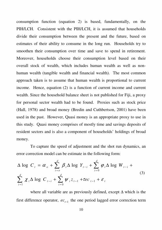
consumption function (equation 2) is based, fundamentally, on the
PIH/LCH. Consistent with the PIH/LCH, it is assumed that households
divide their consumption between the present and the future, based on
estimates of their ability to consume in the long run. Households try to
smoothen their consumption over time and save to spend in retirement.
Moreover, households choose their consumption level based on their
overall stock of wealth, which includes human wealth as well as non-
human wealth (tangible wealth and financial wealth). The most common
approach taken is to assume that human wealth is proportional to current
income. Hence, equation (2) is a function of current income and current
wealth. Since the household balance sheet is not published for Fiji, a proxy
for personal sector wealth had to be found. Proxies such as stock price
(Hall, 1978) and broad money (Bredin and Cuthbertson, 2001) have been
used in the past. However, Quasi money is an appropriate proxy to use in
this study. Quasi money comprises of mostly time and savings deposits of
resident sectors and is also a component of households’ holdings of broad
money.
To capture the speed of adjustment and the shot run dynamics, an
error correction model can be estimate in the following form:
tt
d
i
d
itiiti
d
oi
d
iitiitiot
eczC
WYC
ετψχ
ϕβα
+++∆
+∆+∆+=∆
−= =
−−
= =−−
� �
� �
11 0
1
0
log
logloglog
(3)
where all variable are as previously defined, except ∆ which is the
first difference operator, 1−tec the one period lagged error correction term

11
estimated from equation (2) and tε is the short run error term. The
coefficient on the lagged error correction term measures the speed of
adjustment from a disequilibrium position, which may be brought about as
a result of shock(s) to the system.
Existing consumption literature6 is relied upon to choose the
appropriate variables for Z. In most empirical studies the common
variables considered for Z have been real interest rate, unemployment rate,
and net private transfers.7 The real interest rate is taken to reflect the
substitution effects (time preference for households to consume now or at
sometime in future), while the unemployment rate is considered as a proxy
for uncertainty concerning the future flows of income. Net private transfers
reflect the effects of net migration on consumption.
For the purpose of this study, the choice of the unemployment rate,
real interest rate, and net private transfers are appropriate variables for Z.
These proxies together with contemporaneous as well as lagged
differences of income and wealth, and log of consumption (lagged
difference only) can be specified more specifically as:
tt
d
iiti
d
iiti
d
iiti
d
iitiit
d
ii
d
iitit
ecCptnetrir
urWYC
ετκψω
γρβα
++∆+∆+
++∆+∆+=∆
−=
−=
−=
−
=−−
==−
���
���
1100
0000
log
logloglog (4)
6 Côte and Johnson (1998), Tan and Voss (2000), Sousa (2003). 7 Net private unrequited transfers is calculated as the difference between private transfers credit (immigrant transfers, gifts, maintenance, salaries pension) and private transfers debit (emigrant transfers, gifts and donations, maintenance, and non resident transfers).

12
where ur is the unemployment rate, rir is the real interest rate and
ptnet is the net private transfers. All the other parameters are the same as
defined in equation 3.
Equation (4) is used as a basis for our empirical tests in section 6.
5.0 Methodology
Initially, Engle-Granger (1987) residual based cointegration test is
applied. However, given the limitations of the Engle-Granger approach
when applying to small sample data (as is the case in this study), the
Kremers, Ericcson and Dolado (1992) cointegaration procedure based on
the error correction term t-test is preferred. Kremers et.al (1992) have
argued that residual based cointegration tests are less powerful than test
based on testing the significance of the error correction term in the dynamic
model. The error correction t-test is also shown to have good power even
when the cointegrating vector is moderately miss-specified. Having found
the existence of a cointegarting relationship between consumption, income
and wealth, the long run elasticities are estimated using Ordinary Least
Squares (OLS). Next the short run dynamics are analysed, that is,
analysing how consumption responds to shocks on wealth and income and
how these deviations from the long run relation are correlated. The ECM
specifications are adopted to estimate the short run dynamics.
13
6.0 Empirical Findings
6.1 Data
For the empirical analysis annual time series data form 1979 to
2001 is used. The data is obtained from the Reserve Bank of Fiji, the IMF
International Financial Statistics, and the Fiji Islands Bureau of Statistics
(see Appendix A). Where relevant, all data series were deflated and
expressed in real terms. Actual data was available for all variables except
for the wealth variable where quasi money is used as a proxy.
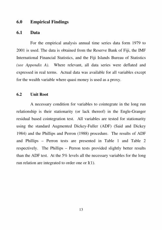
6.2 Unit Root
A necessary condition for variables to cointegrate in the long run
relationship is their stationarity (or lack thereof) in the Engle-Granger
residual based cointegration test. All variables are tested for stationarity
using the standard Augmented Dickey-Fuller (ADF) (Said and Dickey
1984) and the Phillips and Perron (1988) procedure. The results of ADF
and Phillips – Perron tests are presented in Table 1 and Table 2
respectively. The Phillips – Perron tests provided slightly better results
than the ADF test. At the 5% levels all the necessary variables for the long
run relation are integrated to order one or I(1).

14
Table 1: Results of Augmented Dickey – Fuller Tests
Variable ADF Statistics Level Log-level 1st difference
Private Consumption (C) -0.876 -4.575** Disposable Income (Y) -0.269 -6.109** Wealth – Quasi money (W) -1.487 -2.976^ Unemployment (Ur) -2.210 -3.499** Real interest rate (rir) -3.839** 3.939** Net private transfers (ptnet) -1.224 2.936^ Ect-1 -2.717^ Critical Values ** Stationarity at the 1% level (Mackinnon critical values). –3.807 * Stationarity at the 5% level (Mackinnon critical values). –3.019 ^ Stationarity at the 10% level (Mackinnon critical values). –2.650
Table 2: Results of Phillips – Perron Test
Variable PP Statistics Level Log-level 1st difference
Private Consumption (C) -0.899 -4.570** Disposable Income (Y) -0.124 -5.933** Wealth – Quasi money (W) -1.533 -3.013* Unemployment (Ur) -2.615 -4.420** Real interest rate (rir) -2.638 -5.839** Net private transfers (ptnet) -1.124 -2.670^ Ect-1 -2.750^ Critical Values ** Stationarity at the 1% level (Mackinnon critical values). –3.786 * Stationarity at the 5% level (Mackinnon critical values). –3.011 ^ Stationarity at the 10% level (Mackinnon critical values). –2.646

15
6.3 Cointegration
The results of the Engle-Granger (1987) residual test (reported in
Table 1 and Table 2) show that the null hypothesis of no cointegration is
rejected at the 10 percent critical level. The test statistics of the error
correction term lagged one period is –2.717, which exceeds the critical
value of –2.560 (at the 10 percent level) under the ADF test.
An alternative is to use the Kremer et.al (1992) cointegration
method, which is preferred over the Engle Granger (1987). To reject the
null hypothesis of no cointegration, the coefficient of the error correction
term must be significant and have the correct (negative) sign. This is
carried out in the short run regression and the results are reported in Table 4
of section 6.5. The results indicate that the coefficient of the error
correction term is negative and is highly significant at the 1 percent level of
significance (t-statistics of 10.62). This then, confirms that a cointegrating
relationship exists between consumption, income and wealth. The results
of the long run estimation are discussed next.
6.4 Long Run Estimation
The long run model (equation 1) is estimated using OLS. The log
of consumption is regressed against the log of national disposable income
and log of wealth. The results of the regression are presented in table 3.

16
Table 3:Estimated Long Run Model Dependent variable: Log Consumption; estimation period 1979 – 2001
Constant 2.623** (5.387)
Log Income (logY) 0.432** (5.046)
Log Wealth (logW) 0.228** (4.445)
Adjusted R-squared 0.86 SE 0.05
Notes: t-values are in parentheses. **(*) denotes significance at the one(five) per cent levels.
The long run relationships show that both the income variable and
the wealth variable are highly significant, with positive coefficients as
expected. The coefficients of the log-levels of income and wealth can be
interpreted as the long run elasticities of consumption. The estimated long
run elasticity of income is 0.43, about twice as larger than that for wealth
which is around 0.23. In New Zealand, income elasticities ranges from
0.15 to 0.84 (McDermott, 1990;Corfield, 1992;Goh and Downing, 2002),
while the wealth elasticities ranges from 0.21 to 0.39 (McDermott,
1990;Corfield, 1992). For Czech Republic, income elasticity is around
0.51 (Bredin and Cuthbertson, 2001), while in Canada, the income
elasticity and wealth elasticity were 0.89 and 0.32 respectively (Côte and
Johnson, 1998). Consistent with findings in New Zealand, Czech Republic
and Canada, the results obtained for both income elasticity and wealth
elasticity for Fiji are reasonable. Thus, we can interpret the long run
results, as, on average, an increase in income by 1 percent will increase
private consumption by 0.43 percent, while an increase in wealth by 1
percent will increase private consumption by 0.23 percent.

17
6.5 Short Run Estimation
The short run model (equation 3) is estimated using OLS under the
specifications of ECM. Initially, the equation is regressed with difference
of log consumption as the dependent variable against contemporaneous as
well as lagged differences of log income, log wealth, unemployment rate,
real interest rate, net private transfers, and log of consumption (lagged
differences only). A 2-lags structure is employed, as apposed to a 4-lag
structure commonly used by other researchers, due to the limited sample
period. Hendry’s general to specific modelling approach is used at arriving
at a parsimonious model.8 The results of the preferred model are presented
in Table 4.
Table 4: Estimated Parsimonious Short Run Model
Dependent variable: ∆Log Consumption; estimation period 1979 – 2001 Constant 0.109 (11.787)**
∆ logYt 0.380 (9.700)**
∆ logYt-1 0.181 (3.303)**
∆ logYt-2 -0.119 (-2.766)*
∆ logWt 0.256 (7.012)**
∆ logWt-1 -0.009 (-0.413) rirt -0.016 (-12.330)** ∆ptnett-2 -0.039 (-2.223)*
∆ logCt-1 0.064 (0.736) ∆ logCt-2 0.161 (1.780) ect-1 -0.865 (-10.627)**
Adjusted R-squared SE DW
0.950 0.007 2.017
Notes: t-values are in parentheses. **(*) denotes significance at the one(five) per cent levels.
8 Hendry (1987).

18
Turning to error correction specifications, several features of the
regression results stand out. The coefficient on the error correction term
(ect-1) is significant and carries the correct sign. The ECM coefficient
indicates the speed of adjustment and in this case implies a fast adjustment
to the long run relationship. Results suggest that, on average, there is an 87
percent adjustment in the current period (t) to the disequilibrium in the
previous period (t-1). Consumers adjust 87 percent of their consumption to
changes in short run variables when they are certain that the changes in the
variables are permanent in the next period (after a year).
Income growth has a positive contemporaneous effect of
consumption growth, as well as a net positive lagged impact. On average, a
1 percent increase in income growth leads to a 0.38 percent increase in
private consumption within one year, and on balance, a net increase of 0.06
percent in the next two years.
The wealth variable is significant and appears to have a positive
contemporaneous effect on consumption, but no significant lagged impact.
On average, a 1 percent rise in wealth leads to a 0.26 percent increase in
private consumption within a year.
Similarly, the real interest rate variable is also significant and
carries the right sign. A priori, a change in interest rate is expected to have
an impact on consumption, with consumption rising when interest rate falls,
and vice versa. The coefficient suggests that real interest rate has a
negative contemporaneous effect on consumption. On average, a 1 percent
increase in the real interest rate leads to a decline in private consumption by
0.016 percent and vice versa.

19
The change in net private transfers (mostly deficit) has a significant
negative impact on consumption after a two-year lag. This suggests, that if
net private transfers continue to be in deficit, a 1 percent increase would
result in a decrease in private consumption expenditure by 0.039 percent, in
a span of two years.
However, the unemployment rate is not significant and is dropped
from the parsimonious model. This indicates that perhaps households (in
Fiji) smoothen their consumption through periods of uncertainty.
Finally, the fitted and actual values from the parsimonious model
are presented in FIGURE 2. Overwhelmingly, the model fits actual yearly
consumption growth reasonably well, over the period 1979 to 2001.
FIGURE 2 Actual, Fitted and Residual Values from Parsimonious
Short Run Model
-.012
-.008
-.004
.000
.004
.008
-.08
-.04
.00
.04
.08
.12
82 84 86 88 90 92 94 96 98 00
Residual Actual Fitted

20
6.6 Forecasts
To evaluate the forecasting ability of the short run parsimonious
model the out of sample forecasts were constructed. The model is re-
estimated using data for the period 1979-1999. Then, dynamic forecast for
the years 2000 – 2002 is made. FIGURE 3 presents the forecasting
performance of the model with actual out turns over that period.
FIGURE 3 Out of Sample Forecast Evaluation of the
Parsimonious Short Run Model
-.04
-.02
.00
.02
.04
.06
.08
.10
2000 2001 2002
Consumption Forecast
Forecast sample: 2000 2002Included observations: 3
Root Mean Squared Error 0.011696Mean Absolute Error 0.011695Mean Abs. Percent Error 49.15671Theil Inequality Coefficient 0.159009 Bias Proportion 0.105095 Variance Proportion 0.015486 Covariance Proportion 0.879419
The forecast evaluation results indicate that the model has good
forecasting ability. The covariance portion is around 88 percent, indicating
that the model is capable of providing reliable forecasts for the medium
term.9
9 In terms of providing good forecasts it is preferred that the model has a large covariance proportion and a small bias proportion.
21
6.7 Diagnostic Tests
In order for the results to be econometrically creditable, it is
important to investigate the statistical properties of the model. A number of
diagnostic tests have been carried out on the parsimonious short run
model.10
6.7.1 Serial Correlation
Breusch–Godfrey test for first-order serial correlation in our
residuals was performed. There is no significant evidence of the first –
order serial correlation in the residuals. Serial correlation is not present up
to order seven, suggesting that lag structure used in this model is
appropriate.
6.7.2 Normality
The Jarque-Bera LM test is applied. The result of the test shows the
Jarque-Bera statistics is not significant, indicating that the residuals from
the parsimonious short run model are normally distributed.
6.7.3 Other Tests
The model specifications are tested for linearity. Ramsey’s RESET
test 11was applied. The test fails to reject the null hypothesis of linearity in
the parameters, indicating evidence of linearity in the model specification.
The RESET test is also a general test for omitted variables and incorrect
10 See Appendix B, Tables B2 for detailed results on diagnostic tests. 11 RESET stands for Regression Specific Error test, proposed by Ramsey (1969).

22
functional form. The results, suggests that the model specification is
appropriate and the parameters of the model are stable.
7.0 Conclusions
This paper attempted to estimate a consumption function for Fiji in
an error correction framework, to investigate the factors that determine
consumption and for the purpose of forecasting consumption in the medium
term.
The findings reveal the existence of a long run relationship between
consumption, income and wealth, suggesting that consumption is
significantly determined by income and wealth. Consumption elasticities
obtained for income and wealth are reasonable and imply that 43 percent of
the consumers in Fiji are sensitive to changes in current income, in the long
run.
However, in the short run consumption is determined by other
factors other than income and wealth. Real interest rate is highly
significant in determining consumption and appears to have a clear
negative impact on consumption as expected. Net private transfers is also
significant and has a negative impact on consumption with a lag of two
years. Moreover, consumption is more sensitive to contemporaneous
income as indicated by a higher coefficient.
Furthermore, the study also finds that Fiji’s consumption adjusts to
equilibrium levels quite fast. The results suggest that Fiji’s consumers
adjust their consumption behaviour quite early, probably as soon as they

23
gain the slightest indications that the change in their income would be
permanent.
Finally, the results of the forecast evaluation suggest that the short
run model constructed in this study has relatively good forecasting abilities
and can produce a reliable forecast for Fiji’s private consumption in the
medium term.
24
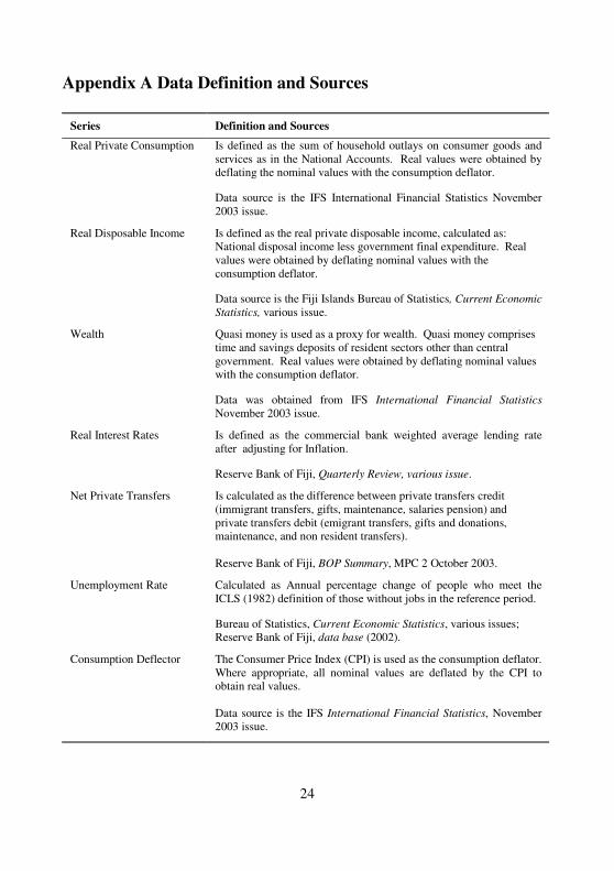
Appendix A Data Definition and Sources
Series Definition and Sources
Real Private Consumption Is defined as the sum of household outlays on consumer goods and services as in the National Accounts. Real values were obtained by deflating the nominal values with the consumption deflator.
Data source is the IFS International Financial Statistics November 2003 issue.
Real Disposable Income Is defined as the real private disposable income, calculated as: National disposal income less government final expenditure. Real values were obtained by deflating nominal values with the consumption deflator. Data source is the Fiji Islands Bureau of Statistics, Current Economic Statistics, various issue.
Wealth Quasi money is used as a proxy for wealth. Quasi money comprises time and savings deposits of resident sectors other than central government. Real values were obtained by deflating nominal values with the consumption deflator.
Data was obtained from IFS International Financial Statistics November 2003 issue.
Real Interest Rates Is defined as the commercial bank weighted average lending rate after adjusting for Inflation.
Reserve Bank of Fiji, Quarterly Review, various issue.
Net Private Transfers Is calculated as the difference between private transfers credit (immigrant transfers, gifts, maintenance, salaries pension) and private transfers debit (emigrant transfers, gifts and donations, maintenance, and non resident transfers). Reserve Bank of Fiji, BOP Summary, MPC 2 October 2003.
Unemployment Rate Calculated as Annual percentage change of people who meet the ICLS (1982) definition of those without jobs in the reference period.
Bureau of Statistics, Current Economic Statistics, various issues; Reserve Bank of Fiji, data base (2002).
Consumption Deflector The Consumer Price Index (CPI) is used as the consumption deflator. Where appropriate, all nominal values are deflated by the CPI to obtain real values. Data source is the IFS International Financial Statistics, November 2003 issue.

25
Appendix B Diagnostic Tests
This appendix presents the results of various diagnostic tests of the
short run error correction model in more detail.
Table B1 presents the pairwise correlation matrix between the
contemporaneous variables contained in the initial and parsimonious
model. The correlations do not appear strong, with the strongest between
the real interest rate and net private transfers at –0.3755. This suggests that
there is no presence of strong multicollinearity in the model. The pairwise
correlation matrix was also done for the lagged variables (not reported),
with similar conclusion.
Table B1: Pairwise Correlation Matrix ∆logWt ∆logYt urt ∆ptnett rirt ∆logWt 1.0000 0.1168 -0.0832 -0.2066 0.1173 ∆logYt 0.1168 1.0000 -0.2626 -0.0364 -0.0420 urt -0.0832 -0.2626 1.0000 -0.0557 -0.1672 ∆ptnett -0.2066 -0.0364 -0.0557 1.0000 -0.3755 rirt 0.1173 -0.0420 -0.1672 -0.3755 1.0000
The results of the tests for normality, serial correlation and
specification error are presented in Table B2. The Jarque-Bera test was
applied to test for normality. The results indicated that the residuals from
the parsimonious model are normally distributed.

26
Table B2: Diagnostics for Parsimonious Short Run Model Probability Normality: Jarque-Bera statistic
χ2 -statistic
1.557
0.459 Serial Correlation: Breusch-Godfrey Serial Correlation LM Test
F-statistic χ2 -statistic
0.217 0.650
0.806 0.722
Specification Error: Ramsey RESET Test
F-statistic LR-statistic
0.868 4.429
0.460 0.109
Notes: **(*) denotes significance at the one (five) per cent levels. LR is a likelihood
ratio statistic.
To test the presence of serial correlation, the Breusch-Godfrey
Lagrange multiplier (LM) test was used. The results (in Table B2) suggest
that serial correlation is not present up to order seven.
Finally, Ramsey’s RESET test was applied to test for specification
error in the model. The results (in Table B2) suggest that there is no
evidence of specification error, thus the model specification is appropriate.

27
References
Banerjee, A., J. Dolado, J.W. Galbraith and D.H. Hendry (1993).
Cointegration, Error-Correction, and the Econometric Analysis of Non-
Stationary Data, Oxford University Press, Oxford.
Blinder, A.R. and A. Deaton (1985). Time Series Consumption Function
Revisited. Brookings Paper on Economic Activity, 2, pp. 465-521.
Bredin, D. and K. Cuthbertson (2001). Liquidity Effects and Precautionary
Saving in the Czech Republic, Central Bank of Ireland Technical Paper
4/RT/01.
Campbell, J. (1987). Does Savings Anticipate a Decline in Labour Income?
An alternative test of the permanent income hypothesis, Econometrica,
55(6), pp. 1249-1273.
Campbell, J. and N. Mankiw (1990). Permanent Income, Current Income,
and Consumption, Journal of Business and economic Statistics 8,
pp.265-279.
Chambers, M.J. (1991). An Alternative Time Series Model of
Consumption: Some empirical evidence, Applied Economics, 23, pp.
1361-1366.
Corfield, I. (1992). Modeling Household Consumption Expenditure in New
Zealand, Reserve Bank of New Zealand Discussion Paper No. G92/9.

28
Côte, D. and M. Johnson (1998). Consumer Attitudes, Uncertainty, and
Consumer Spending, Banque du Canada, Working Paper 98-16.
Davidson, J.E.H. and D.F. Hendry (1981). Interpreting the Econometric
Evidence: The Behavior Consumer’s Expenditure in United Kingdom,
European Economic Review , 16, pp. 177-192.
Davidson, J.E.H., D.F. Hendry., F. Srba. and S. Yeo (1978). Econometric
Modelling of Aggregate Time Series Relationship between Consumers,
Expenditure and Income in United Kingdom, The Economic Journal ,
88, pp. 661-692.
Davis, M.A. (1984). The Consumption Function in Macroeconomic
Models: A comparative study, Applied Economics, 16, pp. 799-838.
Davis, M.A. and M.G. Palumbo (2001). A primer on the Economics and
Time Series Econometrics of Wealth Effects, Federal Reserve Board
Finance and Economic Discussion Paper No. 2001-09.
Deaton, A. (1986). Life-cycle Models of Consumption: Is the evidence
consistent with the theory?, National Bureau of Economic Research
Working Paper No. 1910.
Engle, R.F. and C.W.J. Granger (1987). Co-intergration and Error
Correction: Representation, Estimation and Testing, Econometrica,
55(2), pp. 1039 – 1089.

29
Flavin, M. (1981). The Adjustment of Consumption to Changing
Expectations about future income, Journal of Political Economy, 89,
(5) pp. 974-1009.
Friedman, M. (1957). A Theory of the Consumption Function, Princeton
University Press, Princeton.
Goh, K.L. and R. Downing (2002). Modeling New Zealand Consumption
Expenditure Over the 1990s, New Zealand Treasury Working Paper
02/19.
Hall, R.E. (1978). Stochastic Implications of the Life Cycle Hypothesis:
Theory and Evidence, Journal of Political Economy, 86, pp. 971-987.
Hendry, D.F. (1987). Econometric Methodology: A Personal Perspective,
in T.F. Bewley (ed), Advances in Economics, 2, Cambridge University
Press, pp29-48.
Kremers, J.M., Erricsson, N. R and Dolado, J.J (1992). The Power of
Cointegration Tests, Oxford Bulletin of Economics and Statistics,
54(3), pp. 325-348.
Ludvigson, S. and C. Steindel (1999). How Important is the Stock Market
Effect on Consumption? , Federal Reserve Bank of New York
Economic Policy Review, 5(2), pp. 29-51.

30
Macklem, R.T. ( 1994). Wealth, Disposable Income and Consumption:
Some Evidence from Canada, Bank of Canada, Technical Report No.
71.
Mcdermott, J. (1990). A Time Series Anaylisis of New Zealand Consumer
Expenditure by Durability, Reserve Bank of New Zealand Discussion
Paper No. G90/1.
Modigliani, F. and R. Brumberg (1954). Utility Analysis and the
Consumption Function: An Interpretation of Cross-Section Data, In
Post-Keynesian Economics, ed. K. Kurhira. New Brunswick, NJ:
Rutger University Press.
Molana, H. (1990). The Time Series Consumption Function: Error
Correction, Random Walk and Steady State, Economic Journal, 101,
pp. 382-402.
Muellbauer, J. and R. Lattimore (1995). The Consumption Function: A
Theoretical and Emipirical Overview, in the Handbook of Applied
Econometrics, Volume 1: Macroeconomics edited by M.H. Wickens,
Oxford.
Pindyck, R.S. and D.L. Rubinfeld (1981). Econometric Models and
Economic Forecasts, 2nd ed, McGraw-Hill Book Co., Singapore.
Rae, D. (1997). A Forward Looking Model of Aggregate Consumption in
New Zealand, New Zealand Economic Papers 31(2) pp. 199-220.

31
Tan, A. and G. Voss (2000). Consumption and Wealth, Reserve Bank of
Australia Discussion Paper 2000-09.
Sousa, R.M. (2003). Property of Stocks and Wealth Effects on
Consumption, University of Minho, Department of Economics,
Portugal.
Zeldes, S.P. (1989). Consumption and Liquidity Constraints: An Empirical
Investigation, Journal of Political; Economy, 97, pp. 305-345.