Forecasting Private Consumption: Survey-based Indicators...

Forecasting Private Consumption:

Survey-based Indicators

vs. Google Trends

#155

RUHR

Torsten SchmidtSimeon Vosen

ECONOMIC PAPERS

Imprint

Ruhr Economic Papers

Published by

Ruhr-Universität Bochum (RUB), Department of EconomicsUniversitätsstr. 150, 44801 Bochum, Germany

Technische Universität Dortmund, Department of Economic and Social SciencesVogelpothsweg 87, 44227 Dortmund, Germany

Universität Duisburg-Essen, Department of EconomicsUniversitätsstr. 12, 45117 Essen, Germany

Rheinisch-Westfälisches Institut für Wirtschaftsforschung (RWI)Hohenzollernstr. 1-3, 45128 Essen, Germany

Editors

Prof. Dr. Thomas K. BauerRUB, Department of Economics, Empirical EconomicsPhone: +49 (0) 234/3 22 83 41, e-mail: [email protected]

Prof. Dr. Wolfgang LeiningerTechnische Universität Dortmund, Department of Economic and Social SciencesEconomics – MicroeconomicsPhone: +49 (0) 231/7 55-3297, email: [email protected]

Prof. Dr. Volker ClausenUniversity of Duisburg-Essen, Department of EconomicsInternational EconomicsPhone: +49 (0) 201/1 83-3655, e-mail: [email protected]

Prof. Dr. Christoph M. SchmidtRWI, Phone: +49 (0) 201/81 49-227, e-mail: [email protected]

Editorial Offi ce

Joachim SchmidtRWI, Phone: +49 (0) 201/81 49-292, e-mail: [email protected]

Ruhr Economic Papers #155

Responsible Editor: Christoph M. Schmidt

All rights reserved. Bochum, Dortmund, Duisburg, Essen, Germany, 2009

ISSN 1864-4872 (online) – ISBN 978-3-86788-175-3

The working papers published in the Series constitute work in progress circulated to stimulate discussion and critical comments. Views expressed represent exclusively the authors’ own opinions and do not necessarily refl ect those of the editors.


Torsten Schmidt and Simeon Vosen


Survey-based Indicators

vs. Google Trends


Bibliografi sche Informationen

der Deutschen Nationalbibliothek

Die Deutsche Bibliothek verzeichnet diese Publikation in der deutschen National bibliografi e; detaillierte bibliografi sche Daten sind im Internet über: http//dnb.ddb.de abrufbar.

ISSN 1864-4872 (online)ISBN 978-3-86788-175-3

Torsten Schmidt and Simeon Vosen1


Survey-based Indicators vs. Google Trends

AbstractIn this study we introduce a new indicator for private consumption based on search query time series provided by Google Trends. The indicator is based on factors extracted from consumption-related search categories of the Google Trends applica-tion Insights for Search. The forecasting performance of the new indicator is assessed relative to the two most common survey-based indicators - the University of Michigan Consumer Sentiment Index and the Conference Board Consumer Confi dence Index. The results show that in almost all conducted in-sample and out-of-sample forecast-ing experiments the Google indicator outperforms the survey-based indicators. This suggests that incorporating information from Google Trends may off er signifi cant benefi ts to forecasters of private consumption.

JEL Classifi cation: C53, E21, E27

Keywords: Google Trends, private consumption, forecasting, Consumer Sentiment Indicator

November 2009

1 Both RWI. – This paper initiated in a project proposal to the German Federal Ministry of Finance from May 2009. We thank Roland Döhrn, Max Groneck, Christoph M. Schmidt and the participants of the CIRET/KOF/GKI-Workshop 2009 for helpful comments.– All correspondence to Simeon Vosen, RWI, Hohenzollernstr. 1–3, 45128 Essen, Germany, e-mail: [email protected].

4

1 Introduction

Since private consumption represents about 70 percent of US-GDP, timely

information about private household spending is important to assess and predict overall

economic activity. Data on private consumption for the US are published monthly and

with a lag of one month. Leading indicators with high frequency can therefore be

helpful not only in predicting the future but also the present month (nowcast). The high

frequency and the publication lead of these indicators are of particular usefulness to

economic forecasters in times of macroeconomic turbulences, great uncertainty or

unique shocks when past values of other macroeconomic variables lose predictive

power.

The leading indicators that are typically used to predict consumption are survey-

based sentiment indicators. These indicators try to account for both economic and

psychological1 aspects of consumer behaviour by asking households to assess their own

and the national economy’s current and upcoming economic conditions. The empirical

literature has long noted a strong correlation between consumer sentiment indicators

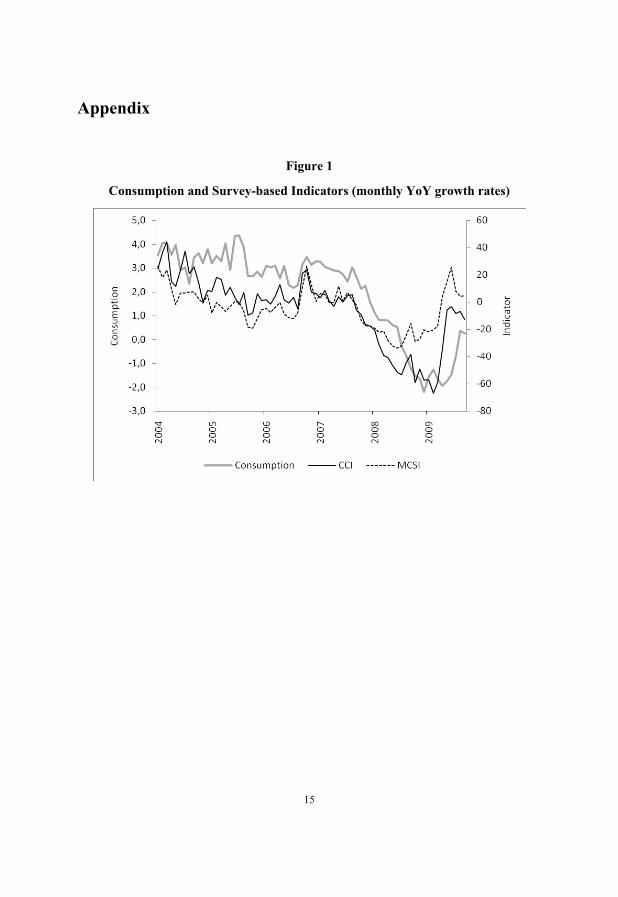
and consumption in the US. Indeed the co-movement of the most common survey-based

consumption indicators – the Michigan University’s Consumer Sentiment Index (MCSI)

and the Conference Board’s Consumer Confidence Index (CCI) – and real consumption

looks quite remarkable although the time-lead of the indicators seems to vary (figure 1).

However, there is little consensus in the empirical literature about these indicators’

ability to collect information that is not already captured in macroeconomic

fundamentals such as income, wealth and interest rates. Fuhrer (1993) finds that roughly

70 percent of the variation in the MCSI can be explained by other macroeconomic

variables, suggesting that large part of sentiment might simply reflect respondents’

knowledge of general economic conditions. A possible weakness of the survey-based

1 See Eppright et al. (1998) for a discussion of arguments from the economic psychology literature on how

consumers’ expectations relate to consumption behavior.

5

indicators could be that they do not accurately capture the link between expectations

and real spending decisions. Carroll et al. (1994) and Ludvigson (2004) find in in-

sample regressions that consumer sentiment indicators nevertheless have explanatory

power for US consumption additional to that contained in other macroeconomic

variables. Other studies, including Croushore (2005) who uses real-time data for out-of-

sample forecasting experiments, find that the MCSI and the CCI are not of significant

value in forecasting consumer spending.

This paper introduces a new indicator for private consumption which is constructed

using data on internet search behaviour provided by Google Trends. Due to the

increasing popularity of the internet it is certain that a substantial amount of people also

use web search engines to collect information on goods they intend to buy. In 2008,

U.S. e-commerce retail sales (excluding travel) totalled $132.3 billion or 3.5% of total

retail sales.2 This share may appear relatively small but the U.S. market research firm

eMarketers estimates that 86% percent of the Internet users are online shoppers, which

means they research and compare but not necessarily purchase products online.3 As a

result, eMarketers estimate store sales influenced by online research to be three times

higher than e-commerce sales. Data about search queries could thus be more related to

spending decisions of private households than sentiment indicators. While

macroeconomic variables indicate consumers’ ability to spend and survey-based

indicators try to capture consumers’ willingness to spend (Wilcox, 2007), the Google

indicator intends to provide a measure for consumers’ preparatory steps to spend by

employing the volume of consumption related search queries. Earlier applications of

Google Trends data include Choi and Varian (2009a and 2009b) who conducted

nowcasting experiments for retail sales, auto sales, home sales, travel and initial

unemployment claims using categories of Google Insights for Search. Ginsberg et al.

(2009) used large numbers of Google Trends search queries to estimate the current level

of influenza activity in the US. Askitas and Zimmermann (2009) found selected queries

2 According to the Quarterly E-Commerce Report of the U.S. Census Bureau, 4th Quarter, 2008. 3 See in “Retail E-Commerce Forecast: Cautious Optimism”, June, 2009, http://www.emarketer.com/Report.aspx?code=emarketer_2000565

6

associated with job search activity to be useful in forecasting the German

unemployment rate. Suhoy (2009) tests for Israel the predictive power of Google Trends

queries for industrial production, retail trade, trade and services revenue, consumer

imports and services exports, as well as employment rates in the business sector.

To use Google data for forecasting private consumption, common unobserved factors

are extracted from time-series of web search categories provided by the Google Trends

application Insights for Search. We assess the new indicator’s usefulness to economic

forecasters by testing to what extent the Google factors improve a simple autoregressive

model compared to common survey-based sentiment indicators. In line with the existing

literature on consumption indicators, any new indicator for private consumption should

also be assessed with regard to its ability to improve forecasting models that already

include other macroeconomic variables. We therefore repeat the exercise using an

extended baseline model that includes several other macroeconomic variables related to

consumer spending. We conduct in-sample and out-of-sample forecasting experiments

using monthly data from January 2005 to September 2009. The results show that in

almost all experiments the Google indicator outperforms the survey-based indicators.

The remainder of this paper is structured as follows: The next section describes the

data and the respective indicators. Section 3 presents the empirical approach to assess

the forecasting performance of the Google indicator. Section 4 discusses the results.

Section 5 concludes.

2 The indicators

Google Trends provides an index of the relative volume of search queries conducted

through Google. The Insights for Search application of Google Trends provides

aggregated indices of search queries which are classified into a total of 605 categories

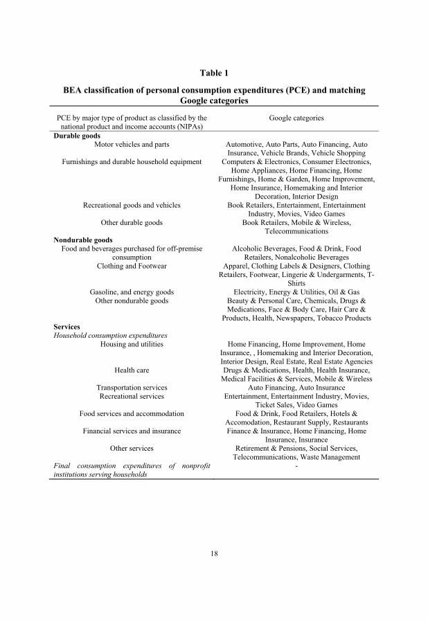
and sub-categories using an automated classification engine.4 We select 56

4 See http://www.google.com/insights/search/?hl=en-US# for a comprehensive description.

7

consumption-relevant categories that in our view are best matches for the product

categories of personal consumption expenditures of the BEA’s national income and

product accounts (Table 1).5 Google Trends data are provided on a weekly basis. We

compute monthly averages since data on consumption are only available on monthly

basis. The Google time-series are not seasonally adjusted. It is, however, hardly

possible to compute accurate seasonal factors since data are available only since 2004

and times have been turbulent in the past 2 years due to the real-estate crisis and the

subsequent financial crisis. We therefore use year on year growth rates instead of

seasonally adjusted data in levels or monthly growth rates. A disadvantage of this

approach is, of course, that we lose 12 months of observations.

To use as many information from the Google data as possible without running out of

degrees of freedom in our forecasting models, we extract common unobserved factors

from the Google data and use these factors as exogenous variables in our regression. To

extract the factors we employ the method of unweighted least squares. The advantage of

this method is that it does not require a positive definite dispersion matrix. This property

is not guaranteed because it is possible that some of the search queries are negatively

correlated. To select the number of factors we initially employed the Kaiser-Guttman

criterion. Depending on the sample period this criterion suggests 11 to 13 factors which

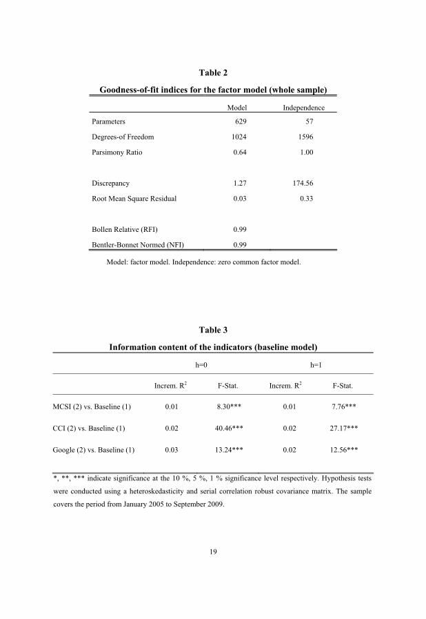
explain between 83 and 94 percent of the variance. The usual indices indicate that the

resulting models fit the data quite well (Table 2). However, with regard to the relatively

short sample period it is necessary to reduce the number of factors further to avoid

overfitting the forecasting models. We therefore estimated equations for each single

factor and for all combinations from two to four factors and perform nowcasts and one-

period-ahead forecasts. The best results were obtained using the four factors with the

largest eigenvalues. In what follows we compare only these four factors with the other

indicators.

5 This approach is based on Choi and Varian (2009a) who assign search categories to components of US retail

sales. We find using search categories more useful for our purposes than specific key words. Specific key words are likely to be more vulnerable to shocks caused by special events unrelated to consumption which could bias the indicator.

8

The survey-based indicators we employ as benchmark indicators are the University

of Michigan’s Consumer Sentiment Index (MCSI) and Conference Board’s Consumer

Confidence Index (CCI). Both indices try to measure the same concept - namely

consumer confidence – and both are based on five questions that include a current

conditions and an expectations component. The main difference is that the CCI puts a

greater weight on labour market conditions whereas the MCSI interviews households

about their financial situation and their current attitude towards major purchases. The

CCI thus slightly lags the MCSI as it is more related to the unemployment rate which

typically lags the business cycle. Due to differences in the construction methodology the

CCI displays also larger movements than the MCSI. As a result of all these differences,

both indicators can give conflicting signals although overall they remain highly

correlated (figure 1).6 For better comparability to the Google indicator we also use year-

on-year growth rates instead of levels of the survey-based indicators.

3 Forecasting experiments

To determine the predictive power of the Google factors relative to that of the

survey-based indicators we first estimate a simple autoregressive model of consumption

growth as a baseline model:

1t h t t hC ( L )C� �� , (1)

where C denotes the monthly year-on-year growth rates of real private consumption

and h is the forecast horizon (0 for nowcasts, 1 for 1-month-ahead forecasts). We use

the Schwarz information criterion to determine the order of the autoregression allowing

up to three lags. Time aggregation and overlapping periods likely introduce an MA(1)

error into the estimation. We therefore model the error term as an MA(1) process.

6 See e.g. Ludvigson (2004) for a more detailed description of the characteristics of these indexes.

9

Next, we add the MCSI, the CCI or the Google Factors to the baseline model to see

to what extent its predictive power is improved by these indicators alone:

1k

t h t t t hC ( L )C ( L )G� � �� , (2)

where Gk is the respective indicator, again allowing up to three lags. To assess

whether these indicators provide information beyond that already captured in other

macroeconomic variables typically embedded in forecasting models, we estimate an

extended baseline model that also includes macroeconomic variables. The selection of

these variables is of course somewhat arbitrary. We employ a model that is also used by

Bram and Ludvigson (1998) and Croushore (2005). It adds to equation (1) real personal

income y, interest rates on three-month treasury bills i and stock prices s (measured by

the S&P 500 index). The last two variables have the advantage of a publication lead of

one month and can thus be used for nowcasting.7 For all macroeconomic variables we

also use year-on-year growth rates.

1 1t h t t t t t hC ( L )C ( L )y ( L )i ( L )s� � �� . (3)

Finally the extended baseline model is again augmented with the respective

indicators:

1 1k

t h t t t t t t hC ( L )C ( L )y ( L )i ( L )s ( L )G� � � �� . (4)

We conduct in-sample and out-of-sample forecasts to determine to what extent the

indicators help to predict movements in consumer spending. In-sample forecasts test the

predictive power of the respective indicator over the entire sample period ranging from

January 2005 to September 2009 while the out-of-sample tests investigate the stability

of that predictive power over several sub-periods. To test which indicator improves the

baseline model best, we calculate the relative reduction in the unexplained variance

(incremental R2) of the respective indicator-augmented equation compared to that of the

baseline models. We also compute the F-statistics to test whether the coefficients of the

7 We use nominal instead of real stock prices to make use of the publication lead of the S&P 500 index. Bram and

Ludvigson (1998) follow Carroll et al. (1994) in using labour income growth instead of personal income growth. For labour income, however, only quarterly data are available.

10

respective indicators and its lags are jointly zero. This test thus shows whether the

relative reduction in unexplained variance is statistically significant.

We use recursive methods for the out-of-sample experiments.8 We first estimate the

models using data from January 2005 to December 2007. Then we conduct out-of-

sample forecasts from January 2008 until September 2009, adding one month at a time,

re-estimating the model and calculating a series of forecasts for the current (nowcast) or

the following month. The forecasts of the indicator augmented models are evaluated by

their respective ratio of the root mean squared forecast errors (RMSFE) to that of the

other models. Significance is determined using the Harvey-Leybourne-Newbold (1997)

modification of the Diebold-Mariano (1995) test statistic.

4 Empirical results

Table 3 displays the results of the in-sample assessment for the indicator-augmented

models (2) relative to baseline model (1) for the sample period ranging from January

2005 to September 2009.9 It reports the increment to the adjusted R2 that results from

augmenting the baseline equation with the respective indicator and the F-statistics for a

test that the coefficients of the indicator and its lags are jointly zero. All indicators

improve the baseline model significantly. The incremental R2s are all of small size,

since we are using overlapping growth rates and lags of the dependent variable already

explain a large share of the variation. The Google-augmented model achieves the

highest incremental R2 of three percentage points for the nowcast and two percentage

points for the one-month-ahead forecast. With an incremental R2 of two percentage

points for both forecast horizons, the CCI indicator performs just slightly worse but the

MCSI indicator is substantially inferior. If the extended baseline model (3) is used as

8 Though a rolling window can better account for structural shifts an expanding window leads to more parameter

stability, precision and it is more realistic for forecasters to use all available data.9 For both survey-based indicators earlier data are also available but to maintain a basis of comparison across

regressions, we use this period as the largest sample for which year-on-year growth rates of all indicators are available.

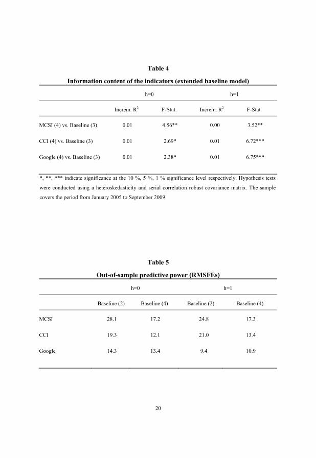
11

the relevant benchmark (table 4), the information content of the indicators diminishes

but remains significant. For both forecast horizons all indicators increase the adjusted

R2 by one percentage point except for the MCSI whose incremental R2 for the one-

month-ahead forecast now falls close to zero.

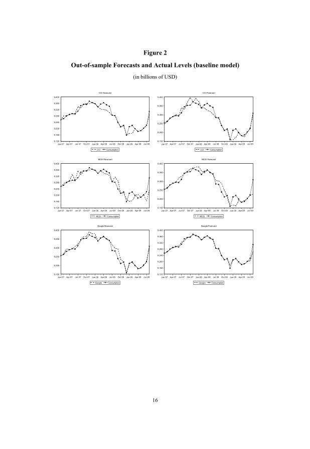
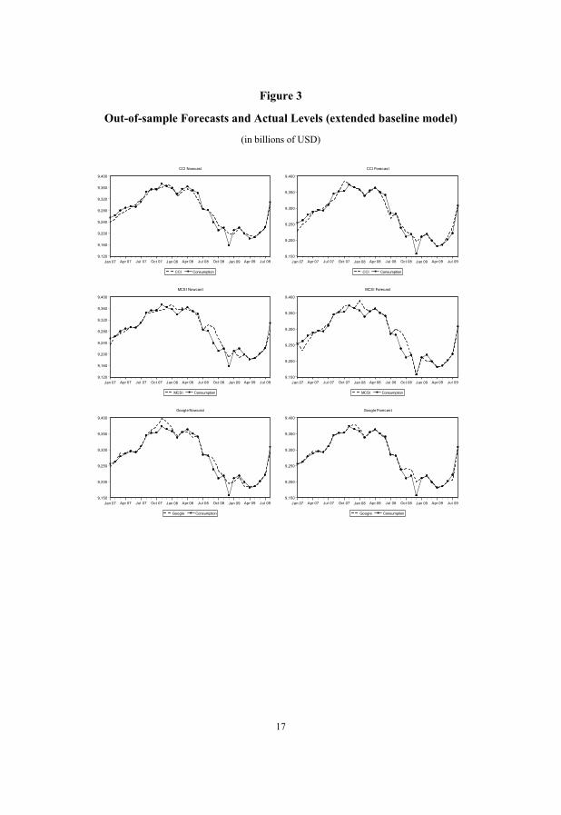
Figures 2 and 3 provide a visual impression of the out-of-sample forecasting

performance of the indicator-augmented models (2) and (4) respectively. Forecasted

values are compared with the actual levels of consumption. Figure 2 shows that the

Google indicator is the only one to accurately indicate the turning point after

consumption had reached its trough in December 2008. The forecasts of the other

models perform particularly badly in the month following the trough. This underlines

that forecasting models should not be based on survey-based indicators alone. The

models augmented with the survey-based indicators obviously perform much better if

macroeconomic variables are included in the baseline models (figure 3). Table 5, in

which the RMSFEs for all indicator-augmented models are reported, supports these

visual impressions. The RMSFEs of the survey-based indicators drop substantially once

other macroeconomic variables are included in the model. For the Google indicator the

picture is less clear. For the nowcasts, including macroeconomic variables slightly

reduces the forecast error. For the one-month-ahead forecasts, however, the reverse is

the case. Interestingly several models perform better in forecasting the next month than

in nowcasting the current month.

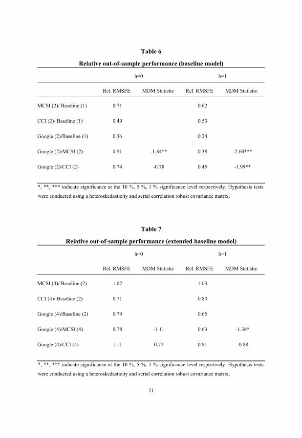
Tables 6 and 7 compare the accuracy of the indicator-augmented models with that of

the baseline models. Additionally, test statistics for equal forecasts accuracy of the

indicator-augmented models are provided. The first entry reports the ratio of the

RMSFE obtained for the MCSI to that for the respective baseline model. The second

entry documents the ratio of the RMSFE for the CCI to that for the baseline model and

so on. The indicator-augmented models are also compared with one another. Entries

lower than one indicate that the first model outperforms the second one. The Diebold-

Mariano (1995) test statistic for equal forecast accuracy modified for small samples by

Harvey, Leybourne and Newbold (1997) appears in the second column. The modified

12

Diebold-Mariano statistics are provided only for the comparisons of the indicator-

augmented models, since they are applicable only to non-nested models. The statistic

has a student’s t-distribution and shows whether differences in RMSFEs are statistically

significant. A negative sign indicates that the first model has a lower forecast error than

the second.

Table 5 shows that if the baseline model is used the Google indicator significantly

outperforms all other models. For the nowcast comparison with the CCI-augmented

model, however, the modified Diebold-Mariano statistic is not significant. If

macroeconomic variables are included (table 7) the relative predictive power of all

indicators deteriorates. For both forecast horizons the MCSI is now even inferior to the

baseline model. For the MCSI our results thus support the findings of Croushore (2005)

that this indicator is not of significant value in forecasting once other macroeconomic

variables are included. The inclusion of the CCI and the Google factors, however, still

reduce the RMSFE of the extended baseline model substantially, the CCI performing

best for the nowcasts and the Google indicator for the one-month-ahead forecasts. The

differences of both forecasting models are however no longer significant.

5 Conclusions

This study shows that Google Trends is a very promising new source of data to

forecast private consumption. In almost all experiments conducted the Google

indicators’ in-sample and out-of-sample predictive power proved to be better than that

of the conventional survey-based indicators. Other methods of category selection might

enhance the indicators predictive power even further. Since 2008 Google also provides

data for product searches specifically and the respective categories should be even more

suitable for consumption forecasts, as they are more related to purchases than the web

search queries that were used here. However, at this point in time there are not even 2

years of data available which forced us to refer to web search categories to obtain at

least 2 years of data. Eventually, employing seasonally adjusted Google data might also

13

be more appropriate than the usage of year-on-year growth rates. We refrained from

seasonal adjustment in this paper, though, since accurate seasonal adjustment requires

more time as well. Given the short time horizon of the data base this paper can thus only

present first insights and there is certainly room for improvements, once longer time-

series are available. The study nevertheless demonstrates the enormous potential that

Google Trends data already offers today to forecasters of consumer spending.

References

Askitas, N. and K. F. Zimmermann, 2009, “Google Econometrics and Unemployment

Forecasting”, Applied Economics Quarterly 55(2), 107-120.

Bram, J. and S. Ludvigson, 1998, “Does Consumer Confidence Forecast Household

Expenditure? A Sentiment Index Horse Race”, Federal Reserve Bank of New York

Economic Policy Review, 59-78.

Carroll, C. D., J. C. Fuhrer and D. W. Wilcox, 1994, “Does Consumer Sentiment

Forecast Household Spending? If So, Why?”, American Economic Review 84, 1397-

1408.

Choi , H. and H. Varian, 2009a, “Predicting the Present with Google Trends”, Google

Technical Report.

Choi , H. and H. Varian, 2009b, “Predicting Initial Claims for Unemployment

Benefits”, Google Technical Report.

Croushore, D., 2005, "Do consumer-confidence indexes help forecast consumer

spending in real time?", The North American Journal of Economics and Finance 16(3),

435-450.

14

Diebold, F. X. and R. S. Mariano, 1995, “Comparing Predictive Accuracy”, Journal of

Business and Economic Statistics 13, 253-263.

Eppright, D. R., N. M. Aguea and W. L. Hunt, 1998, “Aggregate consumer expectation

indexes as indicators of future consumption expenditures”, Journal of Economic

Psychology 19, 215-235.

Fuhrer, J. C., 1993, “What Role does Consumer Sentiment Play in the U.S.

Macroeconomy?”, New England Economic Review January/February, 32-44.

Ginsberg, J., M. H. Mohebbi, R. S. Patel, L. Brammer, M. S. Smolinski and L. Brilliant,

2009, “Detecting Influenza Epedemics using Search Engine Query Data, Nature 457,

1012-1014.

Harvey, D., S. Leyborne and P. Newbold, 1997, “Testing the Equality of Prediction

Mean Squared Errors”, International Journal of Forecasting 13, 281-291.

Ludvigson, S. C., 2004, “Consumer Confidence and Consumer Spending”, Journal of

Economic Perspectives 18(2), 29-50.

Suhoy, T., 2009, “Query Indices and a 2008 Downturn: Israeli Data”, Bank of Israel

Discussion Paper, 2009/06.

Wilcox, J. A., 2007, “Forecasting Components of Consumption with Components of

Consumer Sentiment”, Business Economics 42(2), 36-46.

15

Appendix

Figure 1

Consumption and Survey-based Indicators (monthly YoY growth rates)

16

Figure 2

Out-of-sample Forecasts and Actual Levels (baseline model)

(in billions of USD)

9,120

9,160

9,200

9,240

9,280

9,320

9,360

9,400

Jan 07 Apr 07 Jul 07 Oct 07 Jan 08 Apr 08 Jul 08 Oct 08 Jan 09 Apr 09 Jul 09

CCI Consumption

CCI Nowcast

9,150

9,200

9,250

9,300

9,350

9,400


CCI Consumption

CCI Forecast

9,120

9,160

9,200

9,240

9,280

9,320

9,360

9,400


MCSI Consumption

MCSI Nowcast

9,150

9,200

9,250

9,300

9,350

9,400


MCSI Consumption

MCSI Forecast

9,150

9,200

9,250

9,300

9,350

9,400


Google Consumption

Google Nowcast

9,120

9,160

9,200

9,240

9,280

9,320

9,360

9,400


Google Consumption

Google Forecast

17

Figure 3

Out-of-sample Forecasts and Actual Levels (extended baseline model)

(in billions of USD)

9,120

9,160

9,200

9,240

9,280

9,320

9,360

9,400


CCI Consumption

CCI Nowcast

9,150

9,200

9,250

9,300

9,350

9,400


CCI Consumption

CCI Forecast

9,120

9,160

9,200

9,240

9,280

9,320

9,360

9,400


MCSI Consumption

MCSI Nowcast

9,150

9,200

9,250

9,300

9,350

9,400


MCSI Consumption

MCSI Forecast

9,150

9,200

9,250

9,300

9,350

9,400


Google Consumption

Google Nowcast

9,150

9,200

9,250

9,300

9,350

9,400


Google Consumption

Google Forecast

18

Table 1

BEA classification of personal consumption expenditures (PCE) and matching Google categories

PCE by major type of product as classified by the national product and income accounts (NIPAs)

Google categories

Durable goodsMotor vehicles and parts Automotive, Auto Parts, Auto Financing, Auto

Insurance, Vehicle Brands, Vehicle Shopping Furnishings and durable household equipment Computers & Electronics, Consumer Electronics,

Home Appliances, Home Financing, Home Furnishings, Home & Garden, Home Improvement,

Home Insurance, Homemaking and Interior Decoration, Interior Design

Recreational goods and vehicles Book Retailers, Entertainment, Entertainment Industry, Movies, Video Games

Other durable goods Book Retailers, Mobile & Wireless, Telecommunications

Nondurable goodsFood and beverages purchased for off-premise

consumption Alcoholic Beverages, Food & Drink, Food

Retailers, Nonalcoholic Beverages Clothing and Footwear Apparel, Clothing Labels & Designers, Clothing

Retailers, Footwear, Lingerie & Undergarments, T-Shirts

Gasoline, and energy goods Electricity, Energy & Utilities, Oil & Gas Other nondurable goods Beauty & Personal Care, Chemicals, Drugs &

Medications, Face & Body Care, Hair Care & Products, Health, Newspapers, Tobacco Products

ServicesHousehold consumption expenditures

Housing and utilities Home Financing, Home Improvement, Home Insurance, , Homemaking and Interior Decoration, Interior Design, Real Estate, Real Estate Agencies

Health care Drugs & Medications, Health, Health Insurance, Medical Facilities & Services, Mobile & Wireless

Transportation services Auto Financing, Auto Insurance Recreational services Entertainment, Entertainment Industry, Movies,

Ticket Sales, Video Games Food services and accommodation Food & Drink, Food Retailers, Hotels &

Accomodation, Restaurant Supply, Restaurants Financial services and insurance Finance & Insurance, Home Financing, Home

Insurance, Insurance Other services Retirement & Pensions, Social Services,

Telecommunications, Waste Management Final consumption expenditures of nonprofit institutions serving households

-

19

Table 2

Goodness-of-fit indices for the factor model (whole sample)

Model Independence

Parameters 629 57

Degrees-of Freedom 1024 1596

Parsimony Ratio 0.64 1.00

Discrepancy 1.27 174.56

Root Mean Square Residual 0.03 0.33

Bollen Relative (RFI) 0.99

Bentler-Bonnet Normed (NFI) 0.99

Model: factor model. Independence: zero common factor model.

Table 3

Information content of the indicators (baseline model)

h=0 h=1

Increm. R2 F-Stat. Increm. R2 F-Stat.

MCSI (2) vs. Baseline (1) 0.01 8.30*** 0.01 7.76***

CCI (2) vs. Baseline (1) 0.02 40.46*** 0.02 27.17***

Google (2) vs. Baseline (1) 0.03 13.24*** 0.02 12.56***

*, **, *** indicate significance at the 10 %, 5 %, 1 % significance level respectively. Hypothesis tests

were conducted using a heteroskedasticity and serial correlation robust covariance matrix. The sample

covers the period from January 2005 to September 2009.

20

Table 4

Information content of the indicators (extended baseline model)

h=0 h=1

Increm. R2 F-Stat. Increm. R2 F-Stat.

MCSI (4) vs. Baseline (3) 0.01 4.56** 0.00 3.52**

CCI (4) vs. Baseline (3) 0.01 2.69* 0.01 6.72***

Google (4) vs. Baseline (3) 0.01 2.38* 0.01 6.75***


were conducted using a heteroskedasticity and serial correlation robust covariance matrix. The sample

covers the period from January 2005 to September 2009.

Table 5

Out-of-sample predictive power (RMSFEs)

h=0 h=1

Baseline (2) Baseline (4) Baseline (2) Baseline (4)

MCSI 28.1 17.2 24.8 17.3

CCI 19.3 12.1 21.0 13.4

Google 14.3 13.4 9.4 10.9

21

Table 6

Relative out-of-sample performance (baseline model)

h=0 h=1

Rel. RMSFE MDM Statistic Rel. RMSFE MDM Statistic.

MCSI (2)/ Baseline (1) 0.71 0.62

CCI (2)/ Baseline (1) 0.49 0.53

Google (2)/Baseline (1) 0.36 0.24

Google (2)/MCSI (2) 0.51 -1.84** 0.38 -2.60***

Google (2)/CCI (2) 0.74 -0.78 0.45 -1.99**


were conducted using a heteroskedasticity and serial correlation robust covariance matrix.

Table 7

Relative out-of-sample performance (extended baseline model)

h=0 h=1

Rel. RMSFE MDM Statistic Rel. RMSFE MDM Statistic.

MCSI (4)/ Baseline (2) 1.02 1.03

CCI (4)/ Baseline (2) 0.71 0.80

Google (4)/Baseline (2) 0.79 0.65

Google (4)/MCSI (4) 0.78 -1.11 0.63 -1.38*

Google (4)/CCI (4) 1.11 0.72 0.81 -0.88


were conducted using a heteroskedasticity and serial correlation robust covariance matrix.

Forecasting Private Consumption: Survey-based Indicators...

Documents

Transcript of Forecasting Private Consumption: Survey-based Indicators...