Pontificia Universidad Catolica de ChileFaculty of MathematicsDepartment of Statistics

Modelling predictive validity problems: A partialidentification approach

Eduardo Sebastian Alarcon Bustamante

SUBMITTED IN PARTIAL FULFILLMENT OF THE

REQUIREMENTS FOR THE DEGREE OF

PhD IN STATISTICS

June, 2021

c© Copyright by Eduardo Alarcon-Bustamante, 2021.

All rights reserved. No part of the publication may be reproduced in any form by print, photoprint, microfilm, electronic or any other

means without the prior written permission of one of the copyright holders.

PONTIFICIA UNIVERSIDAD CATOLICA DE CHILE

DEPARTMENT OF STATISTICS

The undersigned hereby certify that they have read and recommend to the Faculty of Mathematics

for acceptance a thesis entitled Modelling predictive validity problems: A partial identificationapproach by Eduardo Sebastian Alarcon Bustamante in partial fulfillment of the requirements

for the degree of PhD in Statistics.

Dated: June, 2021

Research Supervisor :

Ernesto San Martın

Faculty of Mathematics, UC

Research Co-Supervisor :

Jorge Gonzalez

Faculty of Mathematics, UC

Examining Committee :

Sebastien Van Bellegem

Universite catholique de Louvain, Belgium

Xavier de Luna

Umea universitet, Sweden

Kenzo Asahi

School of Government, UC

Isabelle Beaudry

Faculty of Mathematics, UC

PONTIFICIA UNIVERSIDAD CATOLICA DE CHILE

Date: June, 2021

Author : Eduardo Sebastian Alarcon Bustamante

Title : Modelling predictive validity problems: A partial identification approach

Department : Statistics

Degree : PhD in Statistics

Convocation : June

Year : 2021

Permission is herewith granted to Pontificia Universidad Catolica de Chile to circulate and to

have copied for non-commercial purposes, at its discretion, the above title upon the request of

individuals or institutions.

Signature of Author

The author reserves other publication rights, and neither the thesis nor extensive extracts from it

June be printed or otherwise reproduced without the author’s written permission.

The author attests that permission has been obtained for the use of any copyrighted material ap-

pearing in this thesis (other than brief excerpts requiring only proper acknowledgement in scholarly

writing) and that all such use is clearly acknowledged.

IN MEMORY OF MY DAD

Acknowledgements

Firstly, I would like to express my gratitude and admiration to my advisors Ernesto San Martın

and Jorge Gonzalez. They were my guide not only in my thesis but also they were my emotional

support. I will never forget all the grateful moments discussing beyond academic topics. They

were my academic references and they pushed me to who I am now in the research sense.

Secondly, I can not lose the opportunity to thank my mother Marıa Eliana, my brother Daniel,

my sister-in-law Pamela, and my nephews Magdalena and Cristobal. They were very important in

this process. Without their emotional support all it would have been more difficult. At this point, I

would like to thank to all the people that taught me to believe in myself and in my abilities again.

I wish to thank my friends Fabian Chamorro and Alvaro Lara, to believe in me and for all the

de-stress moments biking.

All my gratitude to UC for allowing me access to the data. Finally, I gratefully acknowledge

the financial support of the National Agency for Research and Development (ANID) / Scholarship

Program / Doctorado Nacional / 2018-21181007.

Eduardo Alarcon-Bustamante,

Santiago, June 2021.

Contents

List of tables i

List of figures iii

Introduction iv

The anatomy of the predictive validity problem . . . . . . . . . . . . . . . . . . . . . . iv

Tackling the problem . . . . . . . . . . . . . . . . . . . . . . . . . . . . . . . . . . . . v

Weak ignorability assumption . . . . . . . . . . . . . . . . . . . . . . . . . . . . v

The latent variable model . . . . . . . . . . . . . . . . . . . . . . . . . . . . . . . vi

Partial identification approach . . . . . . . . . . . . . . . . . . . . . . . . . . . . . . . viii

Outline of the dissertation . . . . . . . . . . . . . . . . . . . . . . . . . . . . . . . . . . xi

Final considerations . . . . . . . . . . . . . . . . . . . . . . . . . . . . . . . . . . . . . xi

1 Learning about the predictive validity under partial observability 1

1.1 Introduction . . . . . . . . . . . . . . . . . . . . . . . . . . . . . . . . . . . . . . 1

1.2 Partial identification framework . . . . . . . . . . . . . . . . . . . . . . . . . . . 3

1.2.1 Partial identification of the conditional expectation . . . . . . . . . . . . . 3

1.2.2 Partial identification of the marginal effects . . . . . . . . . . . . . . . . . 4

1.2.3 Identification bounds for marginal effects . . . . . . . . . . . . . . . . . . 6

1.3 Illustration . . . . . . . . . . . . . . . . . . . . . . . . . . . . . . . . . . . . . . . 6

1.3.1 Estimation of the identification bounds . . . . . . . . . . . . . . . . . . . 7

CONTENTS

1.3.2 Results . . . . . . . . . . . . . . . . . . . . . . . . . . . . . . . . . . . . 7

1.4 Conclusions and Discussion . . . . . . . . . . . . . . . . . . . . . . . . . . . . . 8

2 On the marginal effect under partitioned populations: Definition and Interpretation 11

2.1 Introduction . . . . . . . . . . . . . . . . . . . . . . . . . . . . . . . . . . . . . . 11

2.2 Global Marginal Effect . . . . . . . . . . . . . . . . . . . . . . . . . . . . . . . . 13

2.2.1 Definition of the global marginal effect . . . . . . . . . . . . . . . . . . . 13

2.2.2 Interpretation of the global marginal effect . . . . . . . . . . . . . . . . . 14

2.3 Application . . . . . . . . . . . . . . . . . . . . . . . . . . . . . . . . . . . . . . 17

2.3.1 Results . . . . . . . . . . . . . . . . . . . . . . . . . . . . . . . . . . . . 18

2.4 Conclusions and Discussion . . . . . . . . . . . . . . . . . . . . . . . . . . . . . 20

3 On the marginal effect under partially observed partitioned populations: a functionalpredictive validity coefficient 22

3.1 Introduction . . . . . . . . . . . . . . . . . . . . . . . . . . . . . . . . . . . . . . 22

3.1.1 University admission tests in Chile . . . . . . . . . . . . . . . . . . . . . . 25

3.1.2 Data description . . . . . . . . . . . . . . . . . . . . . . . . . . . . . . . 26

3.1.3 Characterisation of the population in study . . . . . . . . . . . . . . . . . 28

3.1.4 Organisation of the chapter . . . . . . . . . . . . . . . . . . . . . . . . . . 29

3.2 Identification bounds for the Conditional expectation . . . . . . . . . . . . . . . . 29

3.3 Identification bounds for the impact of the selection test score over the GPA . . . . 36

3.4 Results from the case-study . . . . . . . . . . . . . . . . . . . . . . . . . . . . . . 45

3.4.1 Estimation of the bounds . . . . . . . . . . . . . . . . . . . . . . . . . . . 45

3.4.2 Results . . . . . . . . . . . . . . . . . . . . . . . . . . . . . . . . . . . . 45

3.5 Conclusions and discussion . . . . . . . . . . . . . . . . . . . . . . . . . . . . . . 49

4 Final conclusions and remarks 51

Appendices 53

CONTENTS

A Proof of the invariant property of the Global Marginal Effect . . . . . . . . . . . . 54

B Proof Proposition 3.2.1 . . . . . . . . . . . . . . . . . . . . . . . . . . . . . . . . 55

C Proof Proposition 3.3.1 . . . . . . . . . . . . . . . . . . . . . . . . . . . . . . . . 56

D Proof for the width, W (x), given in 3.7. . . . . . . . . . . . . . . . . . . . . . . . 60

Bibliography 67

List of Tables

2.1 γz and the empirical proportion of students in undergraduate programs in the fac-

ulty of Biological Sciences. . . . . . . . . . . . . . . . . . . . . . . . . . . . . . . 18

3.1 Application and enrolment status . . . . . . . . . . . . . . . . . . . . . . . . . . . 27

3.2 Minimum, maximum, mean, standard deviation, and median of selection factor

scores for enrolment status of the student. . . . . . . . . . . . . . . . . . . . . . . 28

i

List of Figures

1 Regression under Weak ignorability, Regression under Heckman approach, and

Identification bounds for the regression. . . . . . . . . . . . . . . . . . . . . . . . x

1.1 The regression function and the marginal effect . . . . . . . . . . . . . . . . . . . 5

1.2 Identification bounds for the marginal effect of both Mathematics and Language Test 9

1.2a Identification bounds for marginal effect in Mathematics test. . . . . . . . 9

1.2b Identification bounds for marginal effect in Language and Communication

test. . . . . . . . . . . . . . . . . . . . . . . . . . . . . . . . . . . . . . . 9

2.1 Example situation. The left-side panel shows E(Y |X,Z = z) = δz + γzX .

The right-side panel shows pz(X) = F (uz) for z ∈ {1, 2}, and p0(X) = 1 −∑2z=1 pz(X). . . . . . . . . . . . . . . . . . . . . . . . . . . . . . . . . . . . . . 16

2.2 Functions involved in the Global Marginal Effect . . . . . . . . . . . . . . . . . . 19

2.2a E(Y |X,Z = z) = δz + γzX . . . . . . . . . . . . . . . . . . . . . . . . 19

2.2b pz(X) = F (uz) and p0(X) = 1−2∑z=1

pz(X) . . . . . . . . . . . . . . . . 19

2.2c Conditional Expectation using the Law of Total Probability . . . . . . . . . 19

2.2d Plot of a(X) . . . . . . . . . . . . . . . . . . . . . . . . . . . . . . . . . 19

2.2e Plot of b(X) . . . . . . . . . . . . . . . . . . . . . . . . . . . . . . . . . 19

2.2f Global Marginal Effect . . . . . . . . . . . . . . . . . . . . . . . . . . . . 19

3.1 Boxplots of individual Selection factor score . . . . . . . . . . . . . . . . . . . . . 27

ii

LIST OF FIGURES iii

3.2 Boxplots of the GPA by undergraduate program. . . . . . . . . . . . . . . . . . . . 29

3.3 Identification bounds for both the conditional expectation (left-side) and the Marginal

Effect (right-side) assuming that the System selects correctly. . . . . . . . . . . . . 47

3.3a Identification bounds in the Mathematics test . . . . . . . . . . . . . . . . 47

3.3b Identification bounds in the Language and Communication test . . . . . . . 47

3.3c Identification bounds in the Sciences test . . . . . . . . . . . . . . . . . . 47

3.3d Identification bounds in HGPA selection factor . . . . . . . . . . . . . . . 47

3.3e Identification bounds in Ranking selection factor . . . . . . . . . . . . . . 47

3.4 Identification bounds for both the conditional expectation (left-side) and the Marginal

Effect (right-side) assuming that the System selects wrongly. . . . . . . . . . . . . 49

3.4a Identification bounds in Mathematics test . . . . . . . . . . . . . . . . . . 49

3.4b Identification bounds in Language and Communication test . . . . . . . . . 49

3.4c Identification bounds in Sciences test . . . . . . . . . . . . . . . . . . . . 49

3.4d Identification bounds in HGPA selection factor . . . . . . . . . . . . . . . 49

3.4e Identification bounds in Ranking selection factor . . . . . . . . . . . . . . 49

Introduction

The anatomy of the predictive validity problem

Predictive validity is referred to the relations between test scores and any external variable to the

test (American Educational Research Association et al., 2014). Statistical techniques that have

been used for predictive validity include regression analysis and correlation coefficients between

tests scores, X , and variables that are external to the test, Y (see, Pearson, 1903; Lawley, 1943;

Guilliksen, 1950; Berry et al., 2013; Manzi et al., 2008; Technical Advisory Committee, 2010).

In the context of regression analysis, the conditional expectation of the external variable given the

test scores, namely E(Y |X), is estimated. The predictive validity is assessed through the marginal

effect, which quantifies the changes in this conditional expectation with respect to changes in the

values of the test scores. This approach has been used in several predictive validity studies, for

instance, GU et al. (2008) used the marginal effect to quantify the impact of scores in a patient

satisfaction survey, X , on patients’ medication adherence, Y . Moreover, a result in this study is

that a positive marginal effect of patient satisfaction with pharmacist consultation service reflects

a positive association between patient satisfaction and medication adherence. Thus, if changes in

scores produces large (small) changes in the outcome of interest, then the effect of test scores will

be high (low) on the outcome.

The predictive validity of a test can be evaluated in any field. For example, in Psychiatry, the Beck

Depression Inventory (BDI, Beck et al., 1961) is used to evaluate depression symptoms. The score

in the test gives information about depression level which is categorised into four levels of severity:

Minimal, Mild, Moderate, and Severe. Green et al. (2015) studied the predictive validity of the BDI

Suicide item through a Cox regression model where a conclusion of the study is that the BDI suicide

iv

Introduction v

item significantly predicted both deaths by suicide and repeat suicide attempts. In educational

measurement is common to evaluate the predictive validity of a selection university test (see for

instance Meagher et al., 2006; Makransky et al., 2017; Kobrin et al., 2012). To assess the predictive

validity of them is a statistical challenge because, although the test scores, X , are observed for all

the applicants, the external variable to the test (the Graduate Point Average, GPA, for example), Y ,

is observed only in selected individuals. This problem is accordingly called selection problem and

it arises when the random sampling process does not fully reveal the behaviour of the outcome on

the support of the predictors (Manski, 1993).

From a statistical viewpoint the predictive validity of a selection test, under a regression approach,

can be modelled as follows: let us define a binary random variable S such that S = 1 if the

researcher observes the realisations of Y (e.g. S = 1 if researchers observe the GPA, at the first

year in the University) and S = 0 if not. By using the Law of Total Probability (Kolmogorov,

1950), the conditional expectation is written as:

E(Y |X) = E(Y |X,S = 1)P(S = 1|X) + E(Y |X,S = 0)P(S = 0|X) . (1)

In equation (1), E(Y |X,S = 0) is impossible to be estimated because it is the conditional ex-

pectation of the non-observed outcomes. This fact implies a non-identification of E(Y |X). If

P(S = 0|X) = 0 (i.e. Y is fully observed), the conditional expectation is point identified; how-

ever, in the selection context this probability is not zero. Hence, the conditional expectation is not

identified, and as a consequence the marginal effect is not identified either.

Researchers have devoted a great effort finding restrictions to identify E(Y |X). In what follows,

the statistical strategies that have been used to tackle the identification problem are briefly explained

to introduce the statistical approach in which the proposal is founded.

Tackling the problem

Weak ignorability assumption

Suppose the following identification restriction is imposed: Y ⊥ S|X1 (see Imbens, 2000; Hirano

and Imbens, 2004). To believe in this assumption is analogous to believing in that performance1In words of Florens and Mouchart (1982), Y is conditionally orthogonal to S.

v

Introduction vi

in the non-observed population is equal to the one in the observed population. Formally, this

identification restriction asserts that

E(Y |X,S = 0) = E(Y |X,S = 1). (2)

Equation (2) is a non-refutable assumption, which allow point-identifies E(Y |X) (Manski, 2007).

In fact, it allows making inferences over the conditional expectation ignoring the non-observed

values of the response variable, such that

E(Y |X) = E(Y |X,S = 1). (3)

This approach is widely used in predictive validity studies. To give an example, in Geiser and Stud-

ley (2002) the predictive validity of the SAT scores, X , on the UC freshman grades, Y , was studied

by using the full observed values of both X and Y only. However, because of information about

the non-observed population is not taken into account, the consequence of using this identification

restriction in the predictive validity of a selection test is that it could be underestimated (see Manzi

et al., 2008).

The latent variable model

Suppose that we can identify E(Y |X) by assuming that

E(Y |X) = f1(X)

E(Y |X,S = 1) = f1(X) + f2(X),

for some functions f1 and f2. Suppose that the following specification is introduced: Y is observed

if and only if g(X) + U2 > 0, such that

Y = f1(X) + U1; E(U1|X) = 0

S = 1{g(X)+U2>0}

where f1 and g are real functions of X and (U1, U2) are non-observable random variables. Note

that condition E(U1|X) = 0 allows to interpret f1(X) with respect to the sampling process as

E(Y |X) = f1(X), then:

E(Y |X,S = 1) = E(f1(X) + U1|X,S = 1)

= f1(X) + E(U1|X, g(X) + U2 > 0) .

vi

Introduction vii

A particular case is Heckman’s Selection Model (Heckman, 1976), where

E(Y |X) = X>β1

E(Y |X,S = 1) = X>β1 + ρσφ(X>α)

Φ(X>α).

Here, φ and Φ are the standard normal density and distribution functions, respectively, and ρσ =

E(U1, U2). For details of the estimators of both σ2 and ρXY and its properties see Heckman

(1979)2. In the selection tests context, an example is given in Kennet-Cohen et al. (1999) where

the Heckman’s approach was used for learning about the predictive validity of the Psychometric

Entrance Test for Higher Education in Israel.

From a statistical perspective, imposing a restriction on f1 implies a specification of the function

that characterise the conditional expectation in the whole population, E(Y |X). Nevertheless, an

assumption that restricts this conditional expectation can be incompatible with the reality (Manski,

2003).

It is well-known that statistical inference requires combine the data with assumptions about the

population of interest. In fact, the logic of the inference is:

Data + Assumptions = Conclusions

(see Manski, 2013, p1). Thus, for a fixed data set: when assumptions change, conclusions can

change dramatically. This fact motivate us to define assumptions about the non-observed values in

order to draw more general conclusions for the population of interest. The main objective of this

thesis is learning about both the conditional expectation and the marginal effect by making weaker

assumptions than the standard ones, where it is assumed only one possible scenario: the perfor-

mance in the non-observed group is equal to the one in the observed group. Our proposal is based

on the partial identification approach, whose aim is to find a region to characterise the plausible

solutions that are consistent with the belief the empirical researcher has about these parameters of

interest in the non-observed population. In the partial identification literature, this region is defined

by identification bounds, which are found bounding the non-observed parameter of interest.2Marchenko and Genton (2012) proposed a similar approach on which a t distribution is used instead of a Normal

distribution.

vii

Introduction viii

Partial identification approach

The partial identification approach was introduced by Manski (1989) in an influential paper en-

titled The anatomy of the selection problem. This dissertation is based on two main results of

that paper. The first one is regarding the identification bounds for the conditional expectation,

which are obtained as follows: Assuming that Y ∈ [y0, y1] where y0 ≤ y1, it follows that

y0 ≤ E(Y |X,S = 0) ≤ y1. By applying this inequality to equation (1) we obtain the identifi-

cation region for E(Y |X = x), namely

E(Y |X = x) ∈[E(Y |X = x, S = 1)P(S = 1|X = x) + y0P(S = 0|X = x);

E(Y |X = x, S = 1)P(S = 1|X) + y1P(S = 0|X = x)

](4)

This region characterise all the plausible values for the conditional expectation in presence of non-

observed outcomes by assuming that it is bounded by the range of Y . Note that the width of the

bound is (y1 − y0)P(S = 0|X = x); thus the severity of the identification problem varies directly

with the probability of non-observed outcomes (Manski, 2003). In the context of selection tests,

it is expected that higher scores in the selection test produces high probabilities of observing the

outcome. In contrast, lower scores produce low probabilities of observing the outcome. Thus, the

severity of the identification problem is for lower scores in the selection test.

The second result that we use is regarding the identification bounds for marginal effects, which is

accordingly computed by taking the derivative of E(Y |X) with respect to X . Note that by taking

the derivative with respect to X in (1), we obtain that:

dE(Y |X)

dX=

dE(Y |X,S = 0)

dXP(S = 0|X) + E(Y |X,S = 0)

dP(S = 0|X)

dX

+dE(Y |X,S = 1)

dXP(S = 1|X) + E(Y |X,S = 1)

dP(S = 1|X)

dX. (5)

In Equation (5), both E(Y |X,S = 0) and its derivative are not identified by the data generation

process. The identification bounds for the marginal effect are obtained by combining the assump-

tion of y0 ≤ E(Y |X,S = 0) ≤ y1 with the assumption of that the non-observed derivative exists,

such thatdE(Y |X,S = 0)

dX

∣∣∣∣X=x

∈ [D0x, D1x].

viii

Introduction ix

Thus, by taking into account that in the selection context higher scores produce high probabilities

to observe the outcome of interest (i.e. P(S = 1|X) is an increasing function), it is obtained that:

dE(Y |X)

dX

∣∣∣∣X=x

∈[D0xP(S = 0|X = x) + y0

dP(S = 0|X)

dX

∣∣∣∣X=x

+dE(Y |X,S = 1)

dX

∣∣∣∣X=x

P(S = 1|X) + E(Y |X,S = 1)dP(S = 1|X)

dX

∣∣∣∣X=x

;

D1xP(S = 0|X = x) + y1dP(S = 0|X)

dX

∣∣∣∣X=x

+dE(Y |X,S = 1)

dX

∣∣∣∣X=x

P(S = 1|X) + E(Y |X,S = 1)dP(S = 1|X)

dX

∣∣∣∣X=x

].(6)

To illustrate the approach, and those currently used in the literature, let us consider a selection

test with score scale from 150 to 850, and the GPA with scale from 1.0 to 7.0. In Figure (1) are

shown the results for these three approaches. For the weak ignorability approach, E(Y |X,S = 1)

was estimated by using a Kernel regression as implemented in the npreg function from the np

R-package (Hayfield and Racine, 2008). The Heckman’s model was estimated with the hekit

function from the sampleSelection R-package (Toomet and Henningsen, 2008). Regarding

the identification bounds we used y0 = 1.0 and y1 = 7.0 (the minimum and maximum possible

GPA in this example). The estimation of E(Y |X,S = 1) under the weak ignorability approach

was used. The probability to observe Y , P(S = 1|X), was estimated by using the Probit model

(Bliss, 1934).

From Figure (1), it can be seen that different conclusions can be drawn although the data have not

changed. Note that under the weak ignorability assumption there is a positive relationship between

test scores and the GPA; hence the marginal effect will be a constant function of the scores. From

the Heckman’s viewpoint, this relationship is not linear. Moreover, there is a quadratic relationship

between test scores and the GPA, and therefore the marginal effect will be a non-constant function

of the test scores. When the identification bounds are analysed, assuming that the GPA is bounded

(i.e. 1.0 ≤ GPA ≤ 7.0) we can observe that the severity of the identification problem is for lower

scores. In fact, for selection tests it is expected that for lower scores P(S = 0|X)→ 1. In contrast,

for higher scores it is expected that P(S = 0|X) → 0. Hence, for high scores, the width of the

bounds tend to be the regression line under the ignorability assumption, as well as it is reflected

in Figure (1). Only assuming that E(Y |X,S = 0) is bounded by the range of Y , identification

ix

Introduction x

550 600 650 700 750 800

12

34

56

7

Test score

GPA

Heckman approach

Weak ignorability

Partial identification approach

Figure (1) Regression under Weak ignorability, Regression under Heckman approach, and Iden-

tification bounds for the regression.

bounds give us information about all the plausible solutions for the regression of the GPA on the

test scores.

Note that the regression under weak ignorability, for all test scores, is a plausible solution for

learning about the conditional expectation (it is in between of the bounds). However, the Heck-

man’s model is a non-plausile solution for learning about the conditional expectation when higher

scores are considered. Throughout the document we will give an interpretation of the bounds in the

predictive validity of selection tests context. Despite of we can compute identification bounds for

the conditional expectation by using the range of Y only, the non-observed derivative is not neces-

sarily bounded. Thus, we need to impose identification restrictions by using any criteria which will

allow establish expressions for bothD0x andD1x in the identification region given in Equation (6).

In the partial identification literature there are not results related to establish identification re-

strictions bounding the derivative of the conditional expectation in the predictive validity context.

Thus, this dissertation intends to add to the literature on partial identification by discussing how to

establish identification restrictions by using few general ideas about the problem that a researcher

wants to model.

x

Introduction xi

Outline of the dissertation

The organisation of the dissertation is as follows: in Chapter 1 we intend to set up identification

restrictions for the non-observed marginal effect which are based on a desired property of the

selection tests: higher scores on the test would translate in better performance at higher education.

Nevertheless, the tackled problem in Chapter 1 is based on that the available information comes

from a population that is partitioned into two subpopulations: The outcome is observed, and the

outcome is not observed. Then, a natural extension is when the available information comes from

a population that is partitioned into G groups, where each of them has partial observability of the

outcome. In this context, in Chapter 2 is defined a new way to analyse and interpret the marginal

effect in a partitioned population. The interpretation considers not only the marginal effect in each

group but also the differences in predicted outcomes and the size of the groups. In Chapter 3 we

incorporate the partial observability of the outcome in each group. At this point, we extend the

identification regions given in (4) and (6) to the case of multiple groups, where each of them have

different patterns of missing outcomes. Identification restrictions are based on the beliefs about the

considered selection system. The dissertation ends in Chapter 4 where general conclusions about

the methodology are drawn. Additionally, a generalisation of the proposal is described as a future

work.

Final considerations

The dissertation is a collection of manuscripts that are either published/in press or there are ready

for submission. Hence, there might be some overlapping among the Chapters.

The chapters correspond to the following original manuscripts:

Chapter 1: It is partially based on: Alarcon-Bustamante, E., San Martın, E. & Gonzalez,

J. (2020). Predictive validity under partial observability. In Wiberg, M., Molenaar, M.,

Gonzalez, J., Bockenholt, U., and Kim, JS. (Eds.), Quantitative Psychology. IMPS2019.

Springer Proceedings in Mathematics & Statistics, vol 322. Springer, Cham. DOI 10.1007/978-

3-030-43469-4 11

Chapter 2: It is fully based on: Alarcon-Bustamante, E., San Martın, E. & Gonzalez, J. (in

xi

Introduction xii

press). On the marginal effect under partitioned populations: Definition and Interpretation.

In Wiberg, M., Molenaar, M., Gonzalez, J., Bockenholt, U., and Kim, JS. (Eds.), Quantitative

Psychology. IMPS2020. Springer Proceedings in Mathematics & Statistics.

Chapter 3: Alarcon-Bustamante, E., San Martın, E. & Gonzalez, J. On the marginal effect

under partially observed partitioned populations: a functional predictive validity coefficient

(To be submitted).

xii

Chapter 1

Learning about the predictive validityunder partial observability

1.1 Introduction

A test is used to learn about a behaviour of interest. The relationship between test scores and any

variable external to the test may be used to predict some (future) behaviour of the individuals tested

(Lord, 1980) in the sense that we are interested in the conditional distribution of those external

variables given test scores. We focus our attention on tests that are used in a selection process,

specifically on admission to the higher education. The purpose of the test is to select the “best

applicants” in some specific sense which is typically operationalized through a cut-off score. It is

supposed that the cut-off is defined in such a way that higher scores on the test would translate in

better performance at higher education.

In this context, it is necessary to assess and measure the quality of the selection, which leads to

analyse the validity and reliability of the admission test. Regarding validity, the American Edu-

cational Research Association et al. (2014) define it as the degree to which evidence and theory

support the interpretations of test scores for proposed uses of tests. In particular, the predictive

validity of a test is defined as the evidence based on relations to other variables: in an admission

test, these variables are supposed to be chosen according to the selection purposes of a higher edu-

cational system. Following this definition, the analysis of the relationship between test scores and

1

Chapter 1 2

any external variable to the test provide an important source of predictive validity evidence.

To assess the predictive validity of a selection test is a challenge because the outcome measured

at higher education is observed only in the selected group, whereas the scores of the selection test

are observed for the whole population of applicants. This problem is accordingly called selection

problem and arises when the sampling process does not fully reveal the behavior of the outcome

on the support of the predictors (Manski, 1993).

Statistical procedures used for the evaluation of the predictive validity include regression mod-

els with truncated distributions (Nawata, 1994; Heckman, 1976, 1979; Marchenko and Genton,

2012) and corrected Pearson correlation coefficient (Thorndike, 1949; Pearson, 1903; Mendoza and

Mumford, 1987; Lawley, 1943; Guilliksen, 1950). In the context of admission university selection

tests, a common practice to evaluate the predictive validity of the selection tests is to measure the

correlation between the obtained scores and the cumulative grade point average (GPA) at the first

year of the students in the university.

Although those procedures constitute solutions to the problem of learning about the predictive

validity, it is explicitly assumed a prior knowledge for the performance of the whole population1,

that is, it is assumed that the conditional distribution of the outcome given the scores is known up to

some parameters. However, we argue that this assumption is not pertinent because the consequence

of the partial observability is that the conditional distribution of the outcome given the scores is not

identified and therefore assuming any structure for the non-observed group could not be assessed

empirically (Manski, 1993). For this reason, this approach does not solve satisfactory the problem

of predictive validity. In the educational measurement literature, the predictive validity is typically

analysed through the marginal effect (for instance see Leong, 2007; Goldhaber et al., 2017; Geiser

and Studley, 2002), that is, the derivative of the conditional expectation of the outcome given

scores, with respect to the scores. However, as the conditional expectation is not identified, the

marginal effect is not identified either.

Thus, we propose a methodological approach that allows to learn about the predictive validity of

selection tests through the marginal effects, under partial observability of the outcome. We use a

partial identification approach in order to define a region that characterises the set of all admissible1The term whole population refers to the population that is integrated by two subpopulations: the population where

the outcome is observed and the one where the outcome is not observed (from here on the observed group and the

non-observed group, respectively).

Chapter 1 3

values for the marginal effects. This region is delimited by identification bounds. This approach

works if explicit assumptions on the unobservable distributions are made, the idea being that such

assumptions be weaker than the standard ones above-mentioned (Manski, 2013). We propose to

find identification bounds by assuming that the selection test is such that higher scores would trans-

late to higher values of the outcome, i.e., it is considered that there is a positive relationship between

test scores and the outcome. This assumption reflects an optimistic viewpoint on the selection test

and the idea is to get conclusions to be compared with other perspectives. Identification bounds are

rigorously operationalized through the monotonicity of the conditional expectation of the outcome

given the test score.

The general framework of the partial identification approach is introduced in Section 1.2. In sec-

tion 1.2.1 the partial identification framework of the conditional expectation is formalised. Iden-

tification bounds for marginal effects are formally described in Section 3.3. In Section 1.2.3 the

identification bounds for the marginal effects in the selection problem context are formally char-

acterised. In Section 1.3, the performance of the proposed methodology is illustrated on a real

data set from the selection test used in the university admission Chilean system. Conclusions and

further work are discussed in Section 1.4.

1.2 Partial identification framework

1.2.1 Partial identification of the conditional expectation

Let Y denote the outcome variable, X a test score, and S a binary random variable with S = 1 if

the outcome is observed and S = 0 otherwise. Consequently, each member of the population is

characterized by a triple (Y, S,X). We focused our attention on the conditional expectation of the

outcome Y given a test score X . By the Law of Total Probability (Kolmogorov, 1950), it follows

that

E(Y |X) = E(Y |X,S = 1)P(S = 1|X) + E(Y |X,S = 0)P(S = 0|X) . (1.1)

In (1.1), E(Y |X,S = 1), P(S = 1|X) and P(S = 0|X) are identified by the data generating

process. However, E(Y |X,S = 0) is not identified. Consequently E(Y |X) is not identified either.

One solution for this problem is to assume weak ignorability, namely Y ⊥ S|X2, which implies

2In words, Y ⊥ S|X indicates that Y is conditionally orthogonal to S (see Florens and Mouchart, 1982)

Chapter 1 4

that E(Y |X) = E(Y |X,S = 1). The assumption of weak ignorability allows making inferences

on E(Y |X) ignoring the non-observed values of Y , which can lead to underestimation of the

predictive capacity of the selection test (Manzi et al., 2008).

Assuming that Y ∈ [y0, y1] where y0 and y1 are the minimum and the maximum possible GPA,

respectively, it follows that y0 ≤ E(Y |X,S = 0) ≤ y1. By applying this inequality to equation

(1.1) we have

E(Y |X,S = 1)P(S = 1|X)+y0P(S = 0|X) ≤ E(Y |X)

≤ E(Y |X,S = 1)P(S = 1|X) + y1P(S = 0|X).

The lower bound of the conditional expectation is interpreted as the value E(Y |X) takes if, in

the non-observed group, Y is always equal to y0 (i.e., if all students obtained the worst GPA).

Regarding the upper bound, it is interpreted as the value E(Y |X) takes if, in the non-observed

group, Y is always equal to y1 (i.e., if all students obtained the best GPA) (Manski, 1989).

1.2.2 Partial identification of the marginal effects

As it is well known, the marginal effect is defined as

MEX =dE(Y |X)

dX.

Figure (1.1) shows how variations in X reflect in variations on E(Y |X). These variations arequantified by the change of E(Y |X) with respect to changes in X , defined by MEX . The bluedash lines represent the marginal effect evaluated at the point X = x. From equation (1.1) itfollows that,

MEX =(P(S = 0|X)M.EX

S=0 + P(S = 1|X)M.EXS=1

)+

([E(Y |X,S = 1)− E(Y |X,S = 0)]

dP(S = 1|X)

dX

), (1.2)

where MEXS=s is the marginal effect of X over the group S = s, with z ∈ {0, 1}.

As it was mentioned in Section 2.1, the conditional expectation is not identified in the context of

the selection problem. Consequently, the marginal effect will not be identified either. In fact, in

equation (1.2) both E(Y |X,S = 0) and MEXS=0 are not identified by the sampling process.

In order to find the identification bounds for the marginal effects, suppose thatD0x ≤MEX=xS=0 ≤

D1x, where M.EX=xS=s is the marginal effect of X over the group S = s evaluated at X = x. Thus,

Chapter 1 5

E(Y

|X)

X

E(Y|X)

Marginal effect

Figure (1.1) The regression function and the marginal effect

we assume that the marginal effect for the non selected population exist, which means that if this

population had been selected, the score of the selection test would have predicted the outcome with

an associated marginal effect. This marginal effect is subject to uncertainty, as reflected by the

bounds, which depends on specific values of X .

Considering the above assumption and that y0 ≤ E(Y |X,S = 0) ≤ y1, MEX evaluated atX = x, denoted by MEX=x, is bounded as follows

D0xP(S = 0|X = x)+P(S = 1|X = x)MEX=xS=1 +

[E(Y |X = x, S = 1)− y0]dP(S = 1|X)

dX

∣∣∣∣X=x

≤MEX=x ≤

D1xP(S = 0|X = x)+P(S = 1|X = x)MEX=xS=1 +

[E(Y |X = x, S = 1)− y1]dP(S = 1|X)

dX

∣∣∣∣X=x

Note that an assumption on E(Y |X,S = 0) does not by itself restrict the marginal effect, but

an assumption on both E(Y |X,S = 0) and the marginal effect for the non-observed group, does

(Manski, 1989).

Chapter 1 6

1.2.3 Identification bounds for marginal effects

According to Manski (2003, 2007, 2005), researchers sometimes take credible information about

properties of the outcome. For example, there might be reasons to believe that the outcome in-

crease/decrease monotonically when the predictor increase/decrease. Thus, in a University Admis-

sion System it can be assumed that, from an optimistic view point, a higher score in the selection

test implies a higher GPA at the first year of the university. What can be concluded for the marginal

effect under this optimistic assumption? The partial identification analysis aims to answer this

question.

Selection tests are used to select the best applicants such that higher scores, X , would imply

higher values of the outcome, Y . This fact allows to think that the conditional expectation of

Y given X is a non decreasing function of X and, consequently, the marginal effect in the non-

observed group should be be greater or equal than zero, i.e., MEX=xS=0 ≥ 0. Under this assumption,

it is clear that D0x = 0, and therefore identification bounds for the marginal effect are given by:

P(S = 1|X = x)MEX=xS=1 + [E(Y |X = x, S = 1)− y0]

dP(S = 1|X)

dX

∣∣∣∣X=x

≤MEX=x ≤

D1xP(S = 0|X = x)+P(S = 1|X = x)MEX=xS=1 + [E(Y |X = x, S = 1)− y1]

dP(S = 1|X)

dX

∣∣∣∣X=x

ForD1x, suppose that the predictability ofX over Y in the non-observed group can not be higher

than the maximum observed marginal effect. This assumption is realistic because one objective of

selection tests is to choose those applicants that would obtain a better outcome than those who were

not selected. In terms of and identification restriction for the non-observed marginal effects, this

assumption translates to D1x = maxx∈X

{M.EX=x

S=1

}.

1.3 Illustration

The evolution of the university admission system in Chile includes the baccalaureate test, admin-

istrated during 1931 and 1966; and the Prueba de Aptitud Academica (PAA, for their initials in

Spanish), administered during the period 1967 - 2002. These tests were criticised, among other

reasons, because of their low predictive capacity (Grassau, 1956; DEMRE, 2016; Donoso, 1998).

Chapter 1 7

Since 2004 the selection process is partially based3 on scores from the Prueba de Seleccion Uni-

versitaria (PSU, for their initials in Spanish). The PSU is elaborated based on the secondary

school curriculum and includes two mandatory tests (Mathematics and Language and communica-

tion), and two elective tests (Sciences and History, Geography and Social Sciences). According to

Donoso (1998), one of the reasons for the evolution of the Chilean university admission system is

the necessity to increase predictive capacity of the selection tests.

To illustrate the partial identification approach proposed, we analyse the predictive validity of

the mandatory PSU tests over the GPA of students in the first year in a Chilean university. It is

important to highlight that the analysis is based on the top one university4, so that the assumption

that the performance of non-enrolled students will be at most equal to that of enrolled students, is

tenable.

1.3.1 Estimation of the identification bounds

Let Y denote the GPA and X the score in the selection factor of interest. The conditional expecta-

tion E(Y |X,S = 1) was estimated by an adaptive local linear regression model using a symmetric

Kernel as implemented in the loess.as function from the fANCOVA R-package (Wang, 2010).

The probability of being observed was modeled assuming that P(S = 1|X) = Φ(αX), where

Φ(ν) is the standard normal cumulative probability distribution evaluated at ν. We considered the

standardised values for both X and Y . This means that, by taking into account that in Chile a score

of 1 is the minimum GPA that could be obtained, and a score of 7 the maximum one, we evaluated

our method using y0 = 1−GPAsd(GPA) and y1 = 7−GPA

sd(GPA) , where GPA is the mean of the observed GPA

(5.042) and sd(GPA) is its standard deviation (0.568).

1.3.2 Results

Figures 1.2a, 1.2b and show the identification bounds of the marginal effect for both the Mathe-

matics test and the Language and Communication test. Our method is compared with the marginal

effect of the multiple linear regression model, the traditional procedure that have been used in Chile3Additional to these tests there are other selection factors that are considered in the selection process, namely Ranking

and High school grade point average (NEM)4According to the Quacquarelli Symonds University Rankings 2019.

Chapter 1 8

in order to evaluate the predictive capacity of the selection factors. For this model, the marginal

effect of X is given by its regression coefficient.

For the Mathematics test, it can be seen that the marginal effects are not necessarily a constant

function of the test score. In this case, a higher score produces a higher marginal effect. In other

words, a good performance in the Mathematics test stands for a better performance in the GPA.

Note that these type of conclusions can not be obtained using the traditional procedure. Regarding

the marginal effects for the Language and Communication’s test, contrary to what was seen for the

Mathematics test, the identification bounds are nearly a constant function of the test score. This

means that a good performance in the Language and Communication’s test does not stand for a

better performance in the GPA at the first year.

If a policymaker is ready to believe in these hypothesis, it can be concluded that the marginal

effect computed under ignorability is coherent with them, as well as the case in the Mathematics

test (see Figure 1.2a). In contrast, the multiple linear regression model does not allow to conclude

the marginal effect of the Language and Communication test over the GPA because its marginal

effect is out of the bounds (see Figure 1.2b). Hence, it is a not a plausible solution under the

identification restrictions. Moreover, considering that the marginal effect in this test is lower than

the lowest bound, we can conclude that the current methodological strategy used in Chile is a

non-pertinent solution in the Language and Communication test case

As it was mentioned before, the identification bounds were computed under an optimistic sce-

nario of the selection process. If we assume this scenario for the evaluated undergraduate program,

and a linear regression model is used to extract conclusions about the marginal effect of these

selection tests, it is better to use the Mathematics test instead the Language one.

1.4 Conclusions and Discussion

We have presented a method that allows to learn about the predictive validity of selection tests

through the marginal effect under partial observability.

Our partial identification-type solution characterises the set of all admissible values of the marginal

effect. i.e., if the proposed model for the evaluation of the predictive capacity captures the infor-

mation “the performance of the non-observed group is at most equal to the performance of the

observed group”, then the marginal effect of X must lie between the identification bounds.

Chapter 1 9

−3 −2 −1 0 1

0.0

0.2

0.4

0.6

0.8

Standardized Score in Mathematics Test

Marg

inal effect

Lower bound for Marginal effect Upper bound for Marginal effect Marginal effect multiple linear regression

(a) Identification bounds for marginal effect in Mathematics test.

−3 −2 −1 0 1 2

0.0

0.2

0.4

0.6

0.8

1.0

Standardized Score in Language Test

Marg

inal effect

Lower bound for Marginal effect Upper bound for Marginal effect Marginal effect multiple linear regression

(b) Identification bounds for marginal effect in Language and Communica-

tion test.

Figure (1.2) Identification bounds for the marginal effect of both Mathematics and Language Test

Chapter 1 10

Although other approaches have been proposed to tackle the selection problem by assuming that

the regression line does not change between the observed group and the non-observed group, our

proposal has the advantage of not assuming any parametric structure for the non-observed group, as

we only use properties of the selection tests. More specifically, we used monotonicity assumptions

in order to find the set of all the possible values of the marginal effect by considering that the

selection process is correct. However, this scenario make sense only when information about only

one group with partial observability of the outcome is available. Extending the approach for the

scenario where information about more than one groups is available is a topic that is analysed in

the next Chapters.

Chapter 2

On the marginal effect underpartitioned populations: Definition andInterpretation

2.1 Introduction

In social sciences and other fields, the impact that an exogenous explanatory random variable, X ,

(e.g., the score of a selection test) has on the outcome random variable, Y , (e.g., the cumulative

grade point average, GPA) is usually measured through the marginal effect (see Geiser and Stud-

ley, 2002; DEMRE, 2016; Manzi et al., 2008; Grassau, 1956). The marginal effect quantifies the

changes in the conditional expectation with respect to changes in the values of X: if changes in X

produces large (small) changes in Y , then the effect of X will be high (low) on Y .

In predictive validity studies involving university selection tests, one of the main goals is to

characterise the marginal effect taking into account that the population of interest is partitioned

in groups or clusters (universities, countries, sex, among others). In this context, the conditional

expectation of the GPA is conditioned not only on the test score, but also on a random variable, Z,

characterising the groups. The most common approach is to use a multiple linear regression model

with interaction terms between the test score and the group variable Z. By taking the difference

between the marginal effect of a group of interest and one of reference, researchers compare the

11

Chapter 2 12

impact of the test scores on the GPA between groups. As a matter of fact, the effect that X has

on the group z with respect to the reference, z′, corresponds to the “interaction effect”, which is

quantified by the corresponding interaction regression coefficient (see Cameron and Trivedi, 2005;

Cornelissen, 2005; Powers and Xie, 1999; Norton et al., 2004; Ai and Norton, 2003; Long and

Mustillo, 2018).

Formally, researchers are learning about the marginal effect of X on Y in a partitioned popula-

tion by using the regression E(Y |X,Z), typically a linear one with some interaction terms. Thus,

the analysis is separately made for each group while the interest is to report and draw conclusions

based on a global analysis. As an example, in Miller and Frech (2000) a regression analysis is

used to determine the effect of each explanatory variables on life expectancy measures and infant

mortality for 21 OECD countries. Among the explanatory variables, the authors consider pharma-

ceutical consumption indexes, per capita income and other lifestyle factors such as tobacco use,

alcohol consumption and richness of diet. Their study focuses on both a global analysis, reporting

the effects of the explanatory variables on the outcomes, and an analysis by group, reporting the

marginal effect of some explanatory variables for four countries (France, Italy, US and Ireland). In

this chapter, we will show that this type of analysis needs to be carefully improved, the motivation

being that a trend can appear when different groups are analysed separately, and possibly disappear

when they are combined. This phenomenon is related to the Simpson’s Paradox (see Simpson,

1951; Blyth, 1972).

As a matter of fact, we combine the groups through the Law of Total Probability, which lead

to define E(Y |X) as a mixture of the corresponding conditional expectations for each group with

mixing weights depending on each group. Thus, we compute the marginal effect of X on Y by

using E(Y |X), instead of E(Y |X,Z). We define this marginal effect as the Global Marginal

Effect, which is interpreted as the total marginal effect for partitioned populations. Although from

this result it might be intuitive that the global marginal effect is obtained as a convex combination of

the marginal effects for each group, we show that an additional term that depends on the predictive

outcomes Y ’s by X’s is also included in the definition.

The rest of the chapter is organised as follows. In Section 2.2 the concept of global marginal

effect is formally defined and its properties are discussed. A detailed analysis of the function that

characterise the global marginal effect is also presented in this section. An illustration showing the

use of the global marginal effect in a real data set is presented in Section 2.3. The chapter ends in

Chapter 2 13

Section 3.5 drawing conclusions and with a discussion.

2.2 Global Marginal Effect

2.2.1 Definition of the global marginal effect

Let us consider a population that is partitioned in groups or clusters and for which score data (X,Y )

are observed. Let Z be a categorical random variable such that Z = z if the statistical unit belongs

to the group z for z ∈ {0, . . . , G}. Thus, each member of the population is characterised by a triple

(Y,X,Z). By applying the Law of Total Probability, the conditional expectation, E(Y |X), for the

full population is obtained as

E(Y |X) =∑z

E(Y |X,Z = z)P(Z = z|X). (2.1)

Equation (2.1) provides a global and unique conditional expectation function for the population,

which contains the information of all the groups. In particular, this function could be characterised

as a global model composed of different regression models (one for each group). The component

models are those that relate the scores variables for each group, and a model for the categorical

variable Z. The Global Marginal Effect is accordingly obtained by taking the derivative with

respect to X in Equation (2.1), namely

dE(Y |X)

dX= (2.2)∑

z

dE(Y |X,Z = z)

dXP(Z = z|X) +

∑z

E(Y |X,Z = z)dP(Z = z|X)

dX.

From (2.2), it can be seen that the global marginal effect is not only the weighted average of

the marginal effects in Z = z, but it also depends on the marginal effects observed through the

categorical regression, P(Z = z|X). In particular, it follows that if Z ⊥⊥ X , equation (2.2)

reduces todE(Y |X)

dX=∑z

[dE(Y |X,Z = z)

dX

]P(Z = z).

Thus, the marginal effect in partitioned populations is a weighted average of the marginal effects

in Z = z, if belonging to the group Z does not depend on X .

Chapter 2 14

For the case when Z 6⊥⊥ X , and taking into account that∑

z P (Z = z | X) = 1, the global

marginal effect in Equation (2.2) can be rewritten as follows:

dE(Y |X)

dX=

∑z

dE(Y |X,Z = z)

dXP(Z = z|X) +

+∑z 6=z′

[E(Y |X,Z = z)− E(Y |X,Z = z′)]dP(Z = z|X)

dX; (2.3)

here z′ is the label of a reference group. It can be verified that the global marginal effect is invariant

under the chosen reference group; for a proof, see Appendix A.

Equation (2.3) corresponds to the sum of two functions, namely

a(X) =∑z

dE(Y |X,Z = z)

dXP(Z = z|X), and

b(X) =∑z 6=z′

[E(Y |X,Z = z)− E(Y |X,Z = z′)]dP(Z = z|X)

dX,

where a(X) is a convex combination of the marginal effects in each group with weights being a

function of X . Then, a(X) will vary according to the variations of the weights as a function of X .

The term b(X) is the sum of the differences of the predicted Y , multiplied by the marginal effect

of X on Z.

In the next section, both functions a(X) and b(X) are analysed when the population is assumed to

be partitioned in three groups. A linear and a multinomial logistic regression model are considered

for E(Y |X,Z = z) and P(Z = z|X), respectively.

2.2.2 Interpretation of the global marginal effect

Let us consider three groups, (i.e., z ∈ {0, 1, 2}). By using the invariant property of the global

marginal effect, without loss of generality we take z′ = 0 as the reference group, then

dE(Y |X)

dX=

2∑z=0

dE(Y |X,Z = z)

dXpz(X) +

+

2∑z=1

[E(Y |X,Z = z)− E(Y |X,Z = 0)]dpz(X)

dX,

Chapter 2 15

where pz(X) = P(Z = z|X). If a linear function for E(Y |X,Z = z) is considered (i.e.,

E(Y |X,Z = z) = δz + γzX), the marginal effect is a constant function of X , namely γz .

On the other hand, if a multinomial logistic function F (uz) = exp{uz}/(1 +∑2

j=1 exp{uj}),

uz = αz + βzX and z ∈ {1, 2}, is used for the prediction function, pz(X), the marginal effect of

X on Z is given by

dpz(X)

dX=

pz(X)

(βz −

2∑j=1

βjpj(X)

)if z ∈ {1, 2}

−2∑z=1

pz(X)

(βz −

2∑j=1

βjpj(X)

)if z = 0

(See Wooldridge, 2010; Greene, 2003). This marginal effect inform us about the change in pre-

dicted probabilities due to the changes in X (Wulff, 2014).

Analysis of a(X)

Note that:

a(X) =

2∑z=0

γzpz(X),

which corresponds to a mixture of γz’s with mixing weights defined by p0(X), p1(X), and p2(X).

For ease of exposition, let us consider the following particular case as an example

E(Y |X,Z = 1) ≥ E(Y |X,Z = 0); and E(Y |X,Z = 2) ≥ E(Y |X,Z = 0),

and γ0 > γ2 > γ1. The group 0 has the lowest predicted Y for all the values of X , but its marginal

effect, γ0, is higher than both γ1 and γ2. Hence, its “importance” in a(X) will depends on how

p0(X) varies with respect to X . This case is graphically illustrated in Figure 2.1. From the right-

side panel in Figure 2.1, it can be seen that p0(X) is a decreasing function of X (i.e., for higher

values of X , a lower probability of belonging to the group 0 is found), then for lower values of X ,

a(X) is influenced by γ0p0(X). In this sense, a(X) can be interpreted as a trade-off among the

marginal effects of the groups: as a function of X , it depends not only on the highest value γz for

a specific group z, but also on the size of such a group.

Chapter 2 16

X

Y

Group 0Group 1Group 2

X

P(Z

=z|X

)

Group 0Group 1Group 2

Figure (2.1) Example situation. The left-side panel shows E(Y |X,Z = z) = δz + γzX . The

right-side panel shows pz(X) = F (uz) for z ∈ {1, 2}, and p0(X) = 1−∑2

z=1 pz(X).

Analysis of b(X)

In our example,

b(X) =

2∑z=1

[(δz − δ0) + (γz − γ0)X] (pz(X)[βz(1− pz(X))− βjpj(X)]) ,

with j 6= z. Let us analyse the first component of b(X), namely

b1(X) = [(δ1 − δ0) + (γ1 − γ0)X] (p1(X)[β1(1− p1(X))− β2p2(X)]) .

When

E(Y |X,Z = 1) ≥ E(Y |X,Z = 0),

b1(X) will increase (or decrease) according to

p1(X)[β1(1− p1(X))− β2p2(X)],

which can be written as

p1(X)[β1p0(X)− (β2 − β1)p2(X)]. (2.4)

Note that Equation (2.4) depends not only on the probability of belonging to the group 1, but also

on the probability of belonging to the group 0 and 2. In this context, if x∗1 is the inflection point of

Chapter 2 17

p1(X), which is a monotonic increasing function of X , then for all x > x∗1

P(Z = 1|X = x) > P(Z 6= 1|X = x).

Thus, for all x > x∗1, b1(X) is influenced by P(Z = 1|X = x). In contrast, for all x < x∗1,

b1(X) is influenced by P(Z 6= 1|X = x). For the other groups, the function b(X) can be analysed

analogously.

Collecting all the components of b(X) and after some algebra, it can be shown that

b(X) =2∑z=1

βzpz(X)[fz(X)p0(X) + (fz(X)− fj(X))pj(X)], (2.5)

where z 6= j, and fz(X) = E(Y |X,Z = z) − E(Y |X,Z = 0). Then, b(X) is a function that

depends not only on the differences between the predictions of Y with respect to a reference group,

but also on the probability of being in the groups which in turn change across X .

In summary, the global marginal effect is not only a weighted average of the marginal effects

in each group, but it also considers a term accounting for the differences between the predicted

outcome weighted by the marginal effect of the probability of belonging to the group z. Moreover,

it is not a fixed value as it changes as a function of X . In other words, the global marginal effect

does not reduce to a slope, but it also considers the relevance of the predicted outcomes.

2.3 Application

The university admission system in Chile includes two mandatory selection tests (Mathematics and

Language and Communication) and two elective ones (Sciences and History, Geography and Social

Sciences). Other selection factors, namely, the Ranking and High school GPA are also considered

in the selection process. A score, in the 150-850 scale, is assigned to each selection factor, which

are weighted to obtain a unique application score.

To illustrate the interpretation of the Global Marginal Effect, we analyse the effect of the Mathe-

matics selection test score, X , over the GPA1 in the first year, Y , of selected students in the Faculty

of Biological Sciences of a Chilean university. We analyse the three undergraduate programs of-

fered by this Faculty: Marine Biology, Biochemistry, and Biology. The last enrolled student in

each program scored 631, 631, and 623 in the Mathematics test, respectively.1The scale score for the GPA is 1.0-7.0. The minimum score to pass a course is 4.0.

Chapter 2 18

z Program Prop γz

0 Marine Biology 0.20 0.0096

1 Biochemistry 0.33 0.0072

2 Biology 0.47 0.0074

Table (2.1) γz and the empirical proportion of students in undergraduate programs in the faculty

of Biological Sciences.

To estimate the global marginal effect in equation (2.1), the same functions described in Section

2.2.2 (i.e., a linear function E(Y |X,Z = z) = δz + γzX , and a multinomial logistic model for

pz(X)) were considered. By using the invariant property of the global marginal effect, the chosen

reference group was the Marine Biology program.

2.3.1 Results

To have a general picture on how the global marginal effects varies in terms of test scores, study

programs, and the proportion of students in each program, we used the functions a(X) and b(X)

described in the preceding section. Figure 2.2 shows a graphical representation of both functions

which will be analysed together with the information provided in Table 2.1 that include the estima-

tion of the marginal effects and the proportion of students in each program.

From Table 2.1, it can be seen that the Marine Biology program has the largest marginal effect

and the lowest proportion of students enrolled. In contrast, the smallest marginal effect is found for

the group of students enrolled in the Biochemistry program. Figure 2.2b shows the probability of

belonging to each program as a function of the Mathematics test score. From the figure, it can be

seen that higher score values are associated with higher probabilities of being in the Biochemistry

program (i.e., p1(X) is an increasing function of X). In contrast, p0(X) (the probability of being

in the Marine Biology program), is a decreasing function for all the range of scores. Regarding

the Biology program group, it can be seen that up to a score 619 (approx.), p2(X) is an increasing

function of X that decreases for higher score values. In summary, low scores in the Mathemat-

ics test are associated with a higher probability to find students in the Marine Biology or Biology

Programs than students in Biochemistry. Likewise, higher scores in the Mathematics test are as-

sociated with a higher probability to find students in the Biochemistry than students from Marine

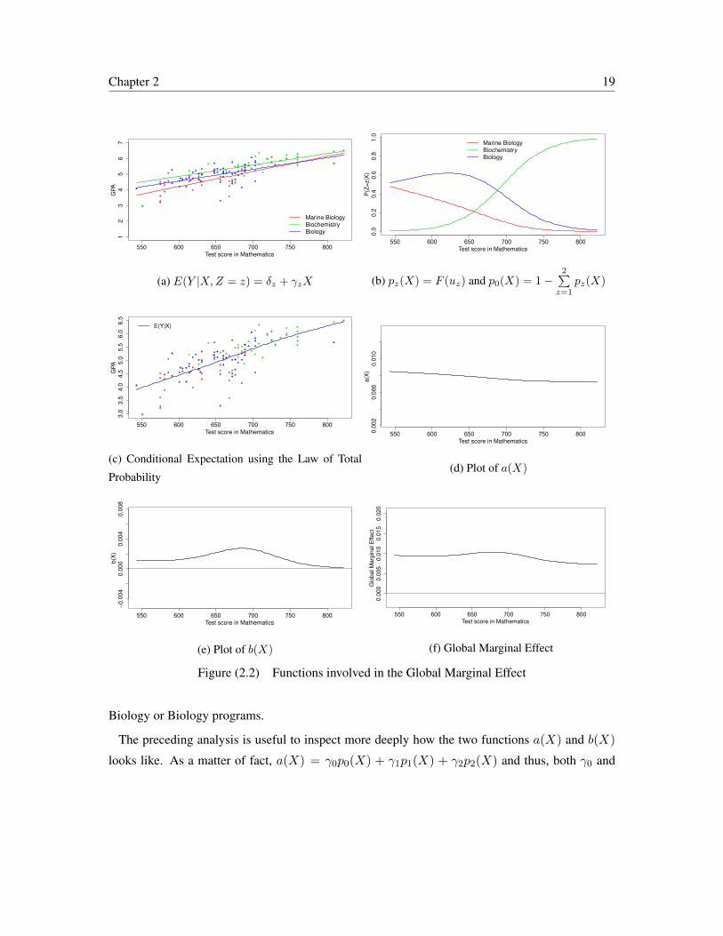
Chapter 2 19

550 600 650 700 750 800

12

34

56

7

Marine BiologyBiochemistryBiology

Test score in Mathematics

GPA

(a) E(Y |X,Z = z) = δz + γzX

550 600 650 700 750 800

0.0

0.2

0.4

0.6

0.8

1.0

Marine Biology

Biochemistry

Biology

Test score in Mathematics

P(Z

=z|X

)

(b) pz(X) = F (uz) and p0(X) = 1−2∑

z=1pz(X)

550 600 650 700 750 800

3.0

3.5

4.0

4.5

5.0

5.5

6.0

6.5

E(Y|X)

Test score in Mathematics

GPA

(c) Conditional Expectation using the Law of Total

Probability

550 600 650 700 750 8000.0

02

0.0

06

0.0

10

Test score in Mathematics

a(X

)

(d) Plot of a(X)

550 600 650 700 750 800

−0

.00

40

.00

00

.00

40

.00

8

Test score in Mathematics

b(X

)

(e) Plot of b(X)

550 600 650 700 750 800

0.0

00

0.0

05

0.0

10

0.0

15

0.0

20

Test score in Mathematics

Glo

ba

l M

arg

ina

l E

ffe

ct

(f) Global Marginal Effect

Figure (2.2) Functions involved in the Global Marginal Effect

Biology or Biology programs.

The preceding analysis is useful to inspect more deeply how the two functions a(X) and b(X)

looks like. As a matter of fact, a(X) = γ0p0(X) + γ1p1(X) + γ2p2(X) and thus, both γ0 and

Chapter 2 20

γ2 have larger weights for lower values of X , while γ1 has a larger weight for higher values of X .

Considering that γ0 > γ2 > γ1, it follows that a(X) is a decreasing function of X as it can be seen

in Figure 2.2d.

Let us analyse b(X) by taking into account Equation (2.5), which can be rewritten as follows:

b(X) = p0(X)(β1p1(X)f1(X) + β2p2(X)f2(X))

+ (β1 − β2)(f1(X)− f2(X))p1(X)p2(X).

Because for low scores in the Mathematics test, p1(X)→ 0, then

b(X)→ β2p0(X)p2(X)f2(X).

On the other hand, for higher values of X , p0(X)→ 0, p2(X)→ 0, then

b(X)→ 0.

Moreover, as it is seen from Figure 2.2a, the score range 619 < x < 703 contains most of the

students from all the programs, and thus b(X) is influenced by p0(X), p1(X), and p2(X), which

is reflected in Figure 2.2e.

The global marginal effect, reported in Figure 2.2f, is the effect that the Mathematics test score

has in students of the Faculty of Biology. For the analysed data, it turns to be positive for the whole

range of test scores. For lower score values, there is a larger proportion of students belonging to a

program where the marginal effect of Mathematics test score is high. In contrast, for higher scores,

a larger proportion of students will be found for a program where the marginal effect is low. Note

that the concavity of the curve in central range of scores is due to the fact that of both f1(X) > 0

and f2(X) > 0 (see Figure 2.2a).

2.4 Conclusions and Discussion

We have introduced the concept of global marginal effect which is obtained by computing the

marginal effect of X on Y by decomposing E(Y |X) with respect to Z through the Law of Total

Probability. The global marginal effect is useful when the main interest is to learn about the effect

of X on Y in a partitioned population.

Chapter 2 21

By means of a physiognomy of the studied population based on Figure 2.2, we have proposed

a new way to analyse and interpret a marginal effect for the case of partitioned populations. Such

interpretation shows the effect of X by considering other characteristics of the population (dif-

ferences in predicted outcomes and the size of each group) which are accordingly defined as a

non-constant function of X . Note that, although the physiognomy of the studied population con-

sidered a particular reference group, the derived result related to the invariant property of the global

marginal effect with respect to the chosen reference group ensures that the type of interpretation

proposed generalises no matter the group chosen as reference.

The studied scenario makes sense if both X and Y are fully observed. In the selection context,

however, there is a partial observability of the outcome, whereas the explanatory random variable

is fully observed (e.g., the GPA in the university is observed in selected students only, whereas the

test scores are observed for all the applicants). In Chapter 3 we combine the results of this Chapter

and the ideas in Chapter 1 in order to have a whole overview of the effect that a selection test score

has over the GPA in the higher education system.

Chapter 3

On the marginal effect under partiallyobserved partitioned populations: afunctional predictive validity coefficient

3.1 Introduction

The impact that an exogenous explanatory random variable, X , has on the outcome random vari-

able, Y is usually measured through the marginal effect, which quantifies the changes in the con-

ditional expectation with respect to changes in the values of X . Several studies have attempted to

measure this impact in a population that is partitioned in groups (sex, countries, age range, among

others). For instance, based on quarantine measures Vasiljeva et al. (2020) conducted a regression

model to assess the impact of the coronavirus pandemic on the economy of some European coun-

tries (Russia, Ukraine, Belarus, Bulgaria, Hungary, Moldova, Poland, Slovakia, Czech Republic).

The analysis is made by country and the impact is reported for the whole Eastern Europe. In fact,

it is concluded that

...GDP in Eastern Europe should be expected to decrease by 6.1% on average as a result of

the COVID-19 pandemic. The main reason for this decline is the decline in production, which

is crucial for all countries except Slovakia..

The necessity to measure the impact of an exogenous random variable, over an outcome of interest

22

Chapter 3 23

is a goal that is not far to the one in predictive validity studies, where the impact that the test

scores, X , have on a random variable of interest, Y is commonly characterised for populations that

are partitioned in groups (universities, programs, occupation, among others). To give an example,

Grobelny (2018) studied, across fifteen occupational groups, the predictive validity of both specific

and general mental ability tests over the job performance. The validity coefficient was analysed for

the whole population (as if only one group existed) as well as for each occupation, where the results

differ substantially with respect to the ones when only the big group is considered. Ayers and Peters

(1977) examined the predictive validity of the Test of English as a Foreign Language, TOEFL, on

the Graduate Record Examination. The subjects of study were students from Republic of China,

India, Thailand, among others. According to the authors, the study does not reveal systematic

differences by country. Thus, the results are reported for the total sample.

In all of these studies, the analysis is separately made for each group while the interest is to re-

port and draw conclusions based on a global analysis. Formally, researchers are learning about

the marginal effect in partitioned populations using the conditional expectation of Y conditioned

not only on X , but also on a random variable, Z, characterising the groups. The most common

approach is to use a multiple linear regression model with interaction terms between X and the

group variable Z. By taking the difference between the marginal effect of a group of interest and

one of reference, researchers compare the impact of X on Y between groups. As a matter of fact,

the effect thatX has on the group z with respect to the reference, z′, corresponds to the “interaction

effect”, which is quantified by the corresponding interaction regression coefficient (see Cameron

and Trivedi, 2005; Cornelissen, 2005; Powers and Xie, 1999; Norton et al., 2004; Ai and Norton,

2003; Long and Mustillo, 2018). Nevertheless, the interest is to draw global conclusions about

the effect of X over Y . In this context, researchers draw conclusions by group and then for the

whole population of interest. However, a trend can appear when different groups are analysed

separately, and possibly disappear when they are combined. This phenomenon is related to the

Simpson’s Paradox (see Simpson, 1951; Blyth, 1972). An alternative analysis for learning about

the marginal effect in partitioned populations is to use the Global Marginal Effect, which is in-

troduced by Alarcon-Bustamante et al. (2021). The authors use the Law of Total Probability to

combine the involved groups and draw conclusions about the predictive validity of a selection test

over the GPA of enrolled students in the Faculty of Biological Sciences of a Chilean university.

The groups are conformed by the three undergraduate programs offered by this Faculty: Marine

Chapter 3 24

Biology, Biochemistry, and Biology.

If both X and Y were fully observed the above mentioned studies make sense; however, an addi-

tional issue arises when conducting predictive validity of selection tests studies: the outcome mea-

sured is partially observed (i.e., it is observed only in the enrolled group), whereas the scores of

the selection test are observed for the whole population of applicants. This problem is accordingly

called selection problem and arises when the sampling process does not fully reveal the behaviour

of the outcome on the support of the predictors (Manski, 1993). A common practice to tackle this

problem is to use available information about both test sores and the outcome of interest. As an

example, Geiser and Studley (2002) conducted a predictive validity study of the SAT scores on the

UC freshman grades for different socioeconomic factors. The authors declare that:

The only exclusions from the sample were students with missing SAT scores or high-school

GPAs; students who did not complete their freshman year and/or did not have a freshman GPA

recorded in the UC Corporate Student Database...

Behind of this analysis, it is assumed a prior knowledge for the performance of the whole popula-

tion. Moreover, it is assumed that the performance in the non-observed group is equal to the one in

the observed groups. This assumption allows making inferences on the conditional distribution of

the outcomes given the scores. However, we argue that this assumption is not pertinent because the

consequence of the partial observability is that the conditional distribution of the outcome given the

scores is not identified and therefore assuming any structure for it could not be assessed empirically

(Manski, 1993). As the conditional distribution is not identified, the conditional expectation is not

identified either. In consequence, the marginal effect is not identified. Based on the partial identi-

fication approach, Alarcon-Bustamante et al. (2020) proposed identification bounds to characterise

the set of all admissible values of the marginal effect under partial observability of the outcome

for the analysis of only one undergraduate program. The bounds were built assuming no specific

structure for the non-observed group, as they only use desired properties of the selection tests.

More specifically, it was assumed that the selection test is such that higher scores would translate

to higher values of the outcome.

Using the partial identification approach, in this chapter we extend the results of Alarcon-Bustamante

et al. (2021) to the partial observability of the outcome case. In fact, we conduct our study with the

full available information: the test score for enrolled and non-enorolled applicants, and the GPA

Chapter 3 25

for the enrolled ones.

The identification bounds for both the conditional expectation and its derivative are rigorously

operationalized through the following assumptions: fisrtly, we use the above-mentioned desired

property of the selection test, i.e., it is considered that there is a positive relationship between test

scores and the outcome. Secondly, we use the objective that the Chilean Unique Admission System

(SUA, for their initials in Spanish) has: select the best applicants according to the obtained scores

in the selection tests (Centro de Estudios, MINEDUC, 2019). The implicit assumption that the

SUA makes is that the selection factors are the unique ones that can predict the performance in the

University. In this context, we found identification bounds under two possible scenarios, namely

The System selects correctly and The System selects wrongly, which were reasoning as follows:

• if the System selects correctly, there are no more factors influencing the predictability of the

outcome. As the SUA assume that the best applicants will be the best in the university, ac-

cording to each selection factor, we assume that the performance of non-enrolled applicants

is at most equal to the one in enrolled students.

• If the System selects wrongly, there are more factors influencing the predictability of the

outcome. Thus, we assume that if only information about the selection test scores is consid-

ered, then the performance of non-enrolled applicants is at least equal to the one in enrolled

students.

Both the desired property of selection tests and the possible scenarios allow us to make identifica-

tion restrictions for both the conditional expectation and its derivative.

Before providing details of the proposed methodology, in the next section we briefly introduce the

motivating case-study and data.

3.1.1 University admission tests in Chile

The evolution of the university admission system in Chile includes four selection tests. The bac-

calaureate test, administrated during the 1931 − 1966 period; the Prueba de Aptitud Academica

(PAA, for their initials in Spanish), administered during the 1967 - 2002 period; The Prueba de

Seleccion Universitaria (PSU, for their initials in Spanish), administrated during the 2004-2019

Chapter 3 26

period. Finally, since 2020 the Prueba de Trancision Universitaria (PTU, for their initials in Span-

ish) is administrated. One of the main reasons for the evolution of the Chilean university admission

system is the necessity to increase predictive capacity of the selection tests (Donoso, 1998).

We focus our study on the predictive validity of the PSU, which was elaborated based on the sec-

ondary school curriculum. The test includes two mandatory tests (Mathematics and Language and

communication), and two elective ones (Sciences and History, Geography and Social Sciences).

Additional to these tests there are other selection factors that are considered in the selection pro-

cess, namely Ranking and High school Grade Point Average (HGPA). A score, in the 150-850

scale, is assigned to each selection factor, which are weighted to obtain a unique application score.

In Chile a student can apply to more than one undergraduate program with his/her test score;

however it can be enrolled in one only. Based on this fact, we induced a partition of the applicants

space as well as is described in Section 3.1.2.

3.1.2 Data description

The data that are used will be based on the PSU, Ranking and HGPA scores for the applicants to

the Faculty of Biological Sciences of a Chilean university, X , and the GPA1 in the first year, Y , of

enrolled students. We analyse the three undergraduate programs offered by this Faculty: Marine

Biology (MB), Biology (B), and Biochemistry (BC). Table (3.1) provides information about how

many students applied to each program, and how many there are enrolled in each one. In this

context, 58.2% of the applicants are not enrolled (NE) in this faculty (which can be considered as

missing values). About the population of enrolled students, 20% there are enrolled in MB, 47.2%

in B, and 32.8% in BC. Table (3.2) provides descriptive statistics for the score in each considered

selection factor2 into each enrolment status. Since the means and medians are very similar for each

variable, for each group, the empirical distributions are fairly symmetric. This fact is reflected in

Figure (3.1), where it can be appreciated that in all the selection factors, there is a tendency to

increase the mean of the scores, such that students enrolled in MB have the minimum mean in each

selection factor, and students enrolled in BC have the maximum one. In Figure (3.2) the boxplot

of the GPA of observed students are shown. The tendency to increase the mean of the scores, such1The scale score for the GPA is 1.0-7.0. The minimum score to pass a course is 4.0.2We did not considered information about the History, Geography and Social Sciences test because we have had an

additional problem related with missing data in the covariates.

Chapter 3 27

Table (3.1) Application and enrolment status

Applied toMB B BC MB & B MB & BC B & BC MB & B & BC

NE 18 41 107 3 0 4 1

Enrolled inMB 21 0 0 2 2 0 0

B 0 52 0 0 0 7 0

BC 0 0 41 0 0 0 0

500

600

700

800

HGPA Language Matem Ranking Sciences

Sel.Factor

Sco

re

Enrollment

NE

MB

B

BC

Figure (3.1) Boxplots of individual Selection factor score

that students enrolled in MB have the minimum mean GPA, and students enrolled in BC have the

maximum one. This tendency is the same than the scores in each selection factor.

Chapter 3 28

Table (3.2) Minimum, maximum, mean, standard deviation, and median of selection factor scores

for enrolment status of the student.

Selection factor Enrolled in n min max x SD Median

Mathematics

NE 174 536 752 627.98 42.74 625

MB 25 575 725 632.16 44.36 631

B 59 543 809 647.24 44.43 652

BC 41 614 822 707.1 45.9 703

Language

NE 174 489 760 618.94 51.19 612

MB 25 517 758 621.96 62.04 620

B 59 523 796 657.61 60.99 654

BC 41 537 807 693.83 67.95 684

Sciences

NE 174 484 768 646.18 47.57 651

MB 25 582 750 642.76 42.23 633

B 59 570 830 682.53 55.64 678

BC 41 660 830 738 46.69 735

HGPA

NE 174 523 785 648.32 53.07 647

MB 25 589 795 668.6 51 678

B 59 564 801 691.02 57.86 698

BC 41 678 816 747.63 36 750

Ranking

NE 174 523 850 682.56 73.35 681.5

MB 25 595 847 703.92 61.73 708

B 59 564 850 733.34 80.09 745

BC 41 701 850 794.68 43.93 801

3.1.3 Characterisation of the population in study

Let us define a random variable Z, where Z = 1 if the student applied to MB only; Z = 2 if

the student applied to B only; Z = 3 if the student applied to BC only; Z = 4 if the student

applied to the both MB and B; Z = 5 if the student applied to the both MB and BC; Z = 6 if the

student applied to the both B and BC, and Z = 7 if the student applied to all the undergraduate

programs. Let S be a random variable that represents the student’s enrolment status, such that

S = 0 if the student is not enrolled; S = 1 if the student is enrolled in MB; S = 2 if the student

is enrolled in B, and S = 3 if the student is enrolled in BC. Note that if a student applied to MB

only (i.e., Z = 1), it can not be enrolled in B or BC. Formally, {{Z = 1} ∩ {S = 2}} = ∅, and

{{Z = 1} ∩ {S = 3}} = ∅. Analogously, a student that applied to both MB and B (i.e., Z = 4),

it can not be enrolled in program BC, i.e., {{Z = 4} ∩ {S = 3}} = ∅. In function of the two

principal characteristics of the selection process: the application and the enrolment status, we have

Chapter 3 29

3

4

5

6

MB B BC

Program

GPA

Program

MB

B

BC

Figure (3.2) Boxplots of the GPA by undergraduate program.

established a partition of the population. In fact,

7∑i=1

3∑j=0

P({Z = i} ∩ {S = j}) = 1,

3.1.4 Organisation of the chapter

The rest of the chapter is organised as follows. In Section 3.2 we introduce the identification

bounds of the conditional expectation in the contexts of the data. Bounds are opertionalised in

both scenarios: the system selects correctly and the system selects wrongly. In Section 3.3 the

identification bounds for the marginal effect are shown in the context of the data. Analogously

to the construction of the bounds for the conditional expectation, we use identification restrictions

that are related with the two possible scenarios for the selection process and the desired property

of the selection tests. Section 3.4 contains the results of the two previous sections from the Chilean

university selection test case study illustrating the benefits of the proposal. The chapter finalises in

Section 3.5 with conclusions and discussion.

3.2 Identification bounds for the Conditional expectation

Let Y be a random variable that represents the GPA. Let X ∈ X be the random variable thatrepresents the score in a selection factor. Let Xij be the space of X in the group S = j, Z = i.Thus, each member of the population is characterised by (Y,X,Z, S). The interest is to learn about

Chapter 3 30

E(Y |X) in this population. By the Law of Total Probability (Kolmogorov, 1950) we have that

E(Y |X) =

7∑i=1

3∑j=0

E(Y |X,Z = i, S = j)P(S = j, Z = i|X)

=

7∑i=1

E(Y |X,Z = i, S = 0)P(S = 0, Z = i|X)

+

7∑i=1

3∑j=1

E(Y |X,Z = i, S = j)P(S = j, Z = i|X) (3.1)

Note that P(S = 0, Z = i|X) is the probability of not being observed in each group. If all the

applicants had enrolled in all i ∈ {1, . . . , 7}, then this probability is zero, and E(Y |X) is equal

to the weighted observed regression, which is given by the second term in the right-side of (3.1).

However, in the selection problem the data generating process is uninformative about the GPA of

non-enrolled students, and therefore E(Y |X,Z = i, S = 0) is impossible to estimate. Provided

that P(S = 0, Z = i|X) 6= 0, the conditional expectation of the population, E(Y |X) is not

identified.

Several statistical procedures have been used to deal with this problem. One solution is to assume

that Y is conditionally orthogonal to S in each Z = i, i.e, Y ⊥ S|X, {Z = i}3 (see Florens and

Mouchart, 1982). This fact allows making inferences on E(Y |X) ignoring the non-observed values

of Y , which can lead to underestimation of the predictive capacity of the selection test (Alarcon-

Bustamante et al., 2020). Other solution is based on regression models with truncated distributions

(for instance, see Nawata, 1994; Heckman, 1976, 1979; Marchenko and Genton, 2012), where it

is explicitly assumed that the conditional distribution of the outcome given the scores is known up

to some parameters. Note that in both cases E(Y |X,S = 0, Z = i) is assumed known, but the

data generation process does not reveal information about it, and therefore the conclusions can be

seriously affected.

According to the ideas of Manski (1989, 2003, 2007, 1993), we can define an identification region

for E(Y |X) when some weaker assumptions about the conditional expectation in the non-observed

group are made. Proposition 3.2.1 give us the identification region for E(Y |X = x) when it is

assumed that E(Y |X,S = 0, Z = i) is bounded:

3It is also known as ignorability assumption.

Chapter 3 31

Proposition 3.2.1. If P(Y ∈ [y0ix, y1ix]|X = x, Z = i, S = 0) = 1, then E(Y |X = x, Z =

i, S = 0) ∈ [y0ix, y1ix], where y0ix ≤ y1ix. Thus, the identification region for E(Y |X = x) is

given by:

E(Y |X = x) ∈

E(Y0x|X = x, S = 0)P(S = 0|X = x) +7∑i=1

3∑j=1

Eji(x)pji(x); (3.2)

E(Y1x|X = x, S = 0)P(S = 0|X = x) +7∑i=1

3∑j=1

Eji(x)pji(x)

where pji(x) = P(S = j, Z = i|X = x), Eji(x) = E(Y |X = x, Z = i, S = j), Y0x =

(y01x, . . . , y07x), and Y1x = (y11x, . . . , y17x)

(see a proof in Appendix B).

The common term in this identification region is E(Y |X = x, S 6= 0) =7∑i=1

3∑j=1

Eji(x)pji(x), the

weighted observed regression. If all applicants had enrolled, P(S = 0|X = x) = 0, thus E(Y |X)

is point identified. Nevertheless, in the selection problem P(S = 0|X = x) > 0, then E(Y |X) is

partially identified (Manski, 2003). Both E(Y0x|S = 0, X = x) and E(Y1x|S = 0, X = x) are

impossible to estimate because applicants in S = 0 there are not enrolled and therefore its GPA is

not observed. Note that y0ix corresponds to the minimum GPA we are ready to believe for non-

enrolled students in each group Z = i, which is a function that depends on the score of enrolled

students (analogously, y1ix corresponds to the maximum one). Thus, E(Y0x|S = 0, X = x) is the

weighted average of the minimum GPA that we are ready to believe in each group, and each score

X = x, which is weighted by the probability of not being enrolled with the correspondent score

X = x, P(S = 0|X = x) (analogously for E(Y1x|S = 0, X = x)). Moreover, the width of the

region is E(Y1x − Y0x|S = 0, X = x)P(S = 0|X = x). Thus the sternness of the identification

problem depends directly on P(S = 0|X = x), the probability of not being observed (Manski,

2003).

Remark 3.2.1. The wider theoretical identification bounds are achieved when y0ix = y0, and

y1ix = y1 (i.e., the minimum and the maximum theoretical GPA, respectively).

The theoretical identification bounds are defined by the minimum and the maximum possible GPA.

By considering that the scale score for the GPA in Chile is 1.0-7.0, we have that y0ix = 1.0 and

Chapter 3 32

y1ix = 7.0. In this case, the lower bound of the conditional expectation is interpreted as the value

E(Y |X) takes if, in the non-enrolled applicants, Y is always equal to y0 = 1.0 (i.e., if all students

obtained the worst GPA). Regarding the upper bound, it is interpreted as the value E(Y |X) takes

if, the non-enrolled applicants, Y is always equal to y1 = 7.0 (i.e., if all students obtained the best

GPA) (Manski, 1989).

Remark 3.2.2. The wider empirical identification bounds are achieved when y0ix = m0i and

y1ix = m1i, the minimum and the maximum observed GPA into the group Z = i, respectivelly .

The empirical identification bounds are defined by the minimum and the maximum observed GPA

in each group Z = i. The lower bound of the conditional expectation is interpreted as the value

E(Y |X) takes if, for each Z = i, S = 0, the GPA, Y , is always equal to the minimum observed

one in Z = i, S 6= 0. The upper bound is interpreted as the value E(Y |X = x) takes if, for each

Z = i, S = 0, the GPA, Y , is always equal to the maximum observed one in Z = i, S 6= 0.

In order to find identification restrictions for E(Y |X,Z = i, S = 0), we write it in terms of the

conditional expectation of the enrolled ones in the same group, i.e., E(Y |X,Z = i, S = 0) is

written in terms of E(Y |X,Z = i, S 6= 0) as follows:

• E(Y |X,Z = i, S = 0) can be written in terms of E(Y |X,Z = i, S = i), for all i ∈ {1, 2, 3}.

• E(Y |X,Z = 4, S = 0) can be written in terms of both E(Y |X,Z = 4, S = 1) and

E(Y |X,Z = 4, S = 2) only.

• E(Y |X,Z = 5, S = 0) can be written in terms of both E(Y |X,Z = 5, S = 1) and

E(Y |X,Z = 5, S = 3) only.

• E(Y |X,Z = 6, S = 0) can be written in terms of both E(Y |X,Z = 6, S = 2) and

E(Y |X,Z = 6, S = 3) only.

• E(Y |X,Z = 7, S = 0) can be written in terms of E(Y |X,Z = 7, S = 1), E(Y |X,Z =

7, S = 2), and E(Y |X,Z = 7, S = 3).

From the empirical point of view, a score in the selection factor, X , can be observed in the group of

non-enrolled applicants even if it is not observed in the group of enrolled students. By taking into

account this issue, in the next sections we define the corresponding y0ix and y1ix in both scenarios:

The system selects correctly, and The system selects wrongly.

Chapter 3 33

Scenario 1: The system selects correctly

If the system selects correctly, we can assume that the performance of non-enrolled applicants

would not be better than the enrolled students. In terms of the conditional expectation, we assume

that, for each Z = i, the not observed expected GPA is at most the the one of an enrolled student

with the same score, X . In fact, for i ∈ {1, 2, 3} we assume that E(Y |X = x, Z = i, S = 0) ≤E(Y |X = x, Z = i, S = i). When i ≥ 3, we can write E(Y |X = i, Z = i, S = 0) in function

of more than one observed conditional expectation. Note that, this identification restriction makes

more informative the upper bound, such that we are assuming that

y0ix ≤ E(Y |X = x, Z = i, S = 0) ≤ E(Y |X = x, Z = i, S 6= 0).

Thus, we define y1ix for all the groups Z = i as follows: let 1{Xji} be a binary random variable,

such that 1{Xji} = 1 if x ∈ Xji and 0 otherwise. Thus, for each X = x, we have that

y1ix :=

E(Y |X = x, Z = i, S = i) · 1{Xii} +m1i · (1− 1{Xii}) if i ∈ {1, 2, 3}

minx∈{X14∪X24}

[E14(x), E24(x)] · 1{X14∪X24} +m14 · (1− 1{X14∪X24}) if i = 4

minx∈{X15∪X35}

[E15(x), E35(x)] · 1{X15∪X35} +m15 · (1− 1{X15∪X35}) if i = 5

minx∈{X26∪X36}

[E26(x), E36(x)] · 1{X26∪X36} +m16 · (1− 1{X26∪X36}) if i = 6

minx∈{X17∪X27∪X37}

[E17(x), E27(x), E37(x)] · 1{X17∪X27∪X37}

+m17 · (1− 1{X17∪X27∪X37}) if i = 7

For each case, we are assuming that if no-enrolled applicant can not be compared with any enrolled

one with the same score X = x, then its expected GPA can not be higher than the maximum

observed one in each group. i.e., y1ix = m1i. Regarding y0ix, we assume that the GPA of a

non-enrolled takes the minimum observed GPA in each group, i.e., y0ix = m0i.

Under these identification restrictions and taking into account Proposal 3.2.1, we have that when it

is assumed that the System chooses correctly:

E(Y0x|X = x, S = 0) =

7∑i=1

m0iP(Z = i|X = x, S = 0),

Chapter 3 34

and

E(Y1x|X = x, S = 0) =

3∑i=1

[Eii(x) · 1{Xii} +m1i · (1− 1{Xii})

]P(Z = i|X = x, S = 0)

+

[min

x∈{X14∪X24}[E14(x), E24(x)] · 1{X14∪X24} +m14 · (1− 1{X14∪X24})

]×P(Z = 4|X = x, S = 0)

+

[min

x∈{X15∪X35}[E15(x), E35(x)] · 1{X15∪X35} +m15 · (1− 1{X15∪X35})

]×P(Z = 5|X = x, S = 0)

+

[min

x∈{X26∪X36}[E26(x), E36(x)] · 1{X26∪X36} +m16 · (1− 1{X26∪X36})

]×P(Z = 6|X = x, S = 0)

+

[min

x∈{X17∪X27∪X37}[E17(x), E27(x), E37(x)] · 1{X17∪X27∪X37}

+m17 · (1− 1{X17∪X27∪X37})

]× P(Z = 7|X = x, S = 0) (3.3)

Scenario 2: The system selects wrongly

In contrast to the above-mentioned scenario, if the system selects wrongly we can assume that the

performance of non-enrolled applicants will be better than the enrolled students. Translated to the

expected GPA, given tests scores in each group, we assume that E(Y |X = x, Z = i, S = 0) ≥E(Y |X = x, Z = i, S = i) for i ∈ {1, 2, 3}. Analogously to the above scenario, we can write

E(Y |X = x, Z = i, S = 0) in function of more than one observed conditional expectation when

i > 3. This scenario allow us to make more informative the lower bound, as we are assuming that

E(Y |X = x, Z = i, S 6= 0) ≤ E(Y |X = x, Z = i, S = 0) ≤ y1ix.

Chapter 3 35

Hence, we define y0ix as follows:

y0ix :=

E(Y |X = x, Z = i, S = i) · 1{Xii} +m0i · (1− 1{Xii}) if i ∈ {1, 2, 3}

maxx∈{X14∪X24}

[E14(x), E24(x)] · 1{X14∪X24} +m04 · (1− 1{X14∪X24}) if i = 4

maxx∈{X15∪X35}

[E15(x), E35(x)] · 1{X15∪X35} +m05 · (1− 1{X15∪X35}) if i = 5

maxx∈{X26∪X36}

[E26(x), E36(x)] · 1{X26∪X36} +m06 · (1− 1{X26∪X36}) if i = 6

maxx∈{X17∪X27∪X37}

[E17(x), E27(x), E37(x)] · 1{X17∪X27∪X37}

+m07 · (1− 1{X17∪X27∪X37}) if i = 7

For each case, we are assuming that if a no-enrolled applicant can not be compared with any

enrolled one with the same score X = x, then its expected GPA can be higher than the minimum

observed one in each group. i.e., y0ix = m0i. Regarding y1ix, we assume that the GPA of a

non-enrolled applicant can takes the maximum observed GPA in each group, i.e., y1ix = m1i.

Under these identification restrictions and taking into account Proposal 3.2.1, we have that when itis assumed that the System selects wrongly:

E(Y0x|X = x, S = 0) =

3∑i=1

[Eii(x) · 1{Xii} +m0i · (1− 1{Xii})

]P(Z = i|X = x, S = 0)

+

[max

x∈{X14∪X24}[E14(x), E24(x)] · 1{X14∪X24} +m04 · (1− 1{X14∪X24})

]×P(Z = 4|X = x, S = 0)

+

[max

x∈{X15∪X35}[E15(x), E35(x)] · 1{X15∪X35} +m05 · (1− 1{X15∪X35})

]×P(Z = 5|X = x, S = 0)

+

[max

x∈{X26∪X36}[E26(x), E36(x)] · 1{X26∪X36} +m06 · (1− 1{X26∪X36})

]×P(Z = 6|X = x, S = 0)

+

[max

x∈{X17∪X27∪X37}[E17(x), E27(x), E37(x)] · 1{X17∪X27∪X37}

+m07 · (1− 1{X17∪X27∪X37})

]× P(Z = 7|X = x, S = 0), (3.4)

and

E(Y1x|X = x, S = 0) =

7∑i=1

m1iP(Z = i|X = x, S = 0).

In summary, we have proposed identification bounds for the conditional GPA in this partitioned

population in two possible scenarios. The wider bounds are achieved using the range of possible

Chapter 3 36

values of the GPA in both theoretical and empirical cases. The assumptions regarding the belief

about the correctness the system has to select the applicants allow us to make more informative the

bounds. In fact, if we are ready to believe that the System selects correctly, then the upper bound

will be more informative. In contrast, if we are ready to believe that the System selects wrongly,

then the lower bound will be more informative.

In the next section we provide identification bounds for the marginal effect of the selection fac-

tor scores over the GPA, which is considered as a validity coefficient for them. The bounds are

operacionalized taking into account the same scenarios than for the conditional expectation.

3.3 Identification bounds for the impact of the selection test scoreover the GPA

The effect that the score, X , has on the outcome random variable of interest, Y , is usually mea-

sured through the marginal effect, which is accordingly defined as the derivative of the conditional

expectation, E(Y |X), with respect to X , namely:

MEX =dE(Y |X)

dX.

In our context, we need to characterise the marginal effect in a population that is partitioned by the

application status and the enrolment one.

We know that each Z = i is partitioned by S, where S ∈ {0, 1, 2, 3}. According to the ideas of

Alarcon-Bustamante et al. (2021), where the marginal effect for partitioned populations is defined,

namely Global Marginal Effect (GME), we have that

MEX =7∑i=1

3∑j=0

dE(Y |X,Z = i, S = j)

dXP(S = j|X,Z = i)

+

3∑j=1

[E(Y |X,Z = i, S = j)− E(Y |X,Z = i, S = 0)]

× dP(S = j|X,Z = i)

dX

]P(Z = i|X)

+

7∑i=1

3∑j=0

E(Y |X,Z = i, S = j)P(S = j|X,Z = i)

dP(Z = i|X)

dX. (3.5)

Chapter 3 37

Intuitively, the marginal effect in this partitioned population is the weighted average of each GME

in Z = i. However, from (3.5), it can be seen that an additional term, related with the expected

GPA in each Z = i, and the marginal marginal effect observed through the categorical regression,

P(Z = i|X), appears. In particular, it follows that if Z ⊥⊥ X (i.e., if the application status of the

student does not depend on the obtained score, X), equation (3.5) reduces to a weighted average

of each GME (wGME). However, in the selection process this fact does not make sense because

the student applies according to the obtained score, hence we can assume that Z 6⊥⊥ X . For

each Z = i, by considering the non-enrolled group as the reference one, the GME is computed,

and it is weighted by the probability of belong to each Z = i. Note that if S ⊥⊥ X|{Z = i} (i.e.,

enrolment status does not depend on the score,X in each application status Z = i), then each GME

corresponds to the weighted average marginal effect. However, in the selection process context this

fact does not make sense because for all Z = i, the students are enrolled (or not) according to the

the obtained score. Assuming that S 6⊥⊥ X|{Z = i}, it can be seen that the wGME depends not

only on the GME in each group, but also on the differences of the predicted GPAs with respect

to the one of the non-enrolled applicants. Nevertheless, both the last quantity and its derivative,

are impossible to obtain because the GPA of the non-enrolled applicants is not observed. This fact

relies on a non identification of MEX . A possible solution is to use the observed information only

as well as the above mentioned procedures, and compute the derivative of E(Y |X,Z = i, S 6= 0)

through with respect to X . However, assuming any structure for the non-observed quantities can

seriously affect the conclusions.

In order to use the partial identification approach, it is important to highlight that a bound on Y

does not by itself restrict the marginal effect. A bound on Y combined with one on the marginal ef-

fect for non-enrolled applicants does (Manski, 1989). In this context, we combine the identification

restriction in Proposition 3.2.1 with an assumption on the non-observed marginal effect. In fact,

we assume that the marginal effect for the non-enrolled population exist for each Z = i (i.e., the

marginal effect is bounded, which means that if this population had been enrolled, the score of the

selection test would have predicted the outcome with an associated marginal effect). Following the

ideas of Manski (1989). Proposition 3.3.1 give us the identification region for the marginal effect:

Proposition 3.3.1. Let us suppose that y0ix ≤ E(Y |X,Z = i, S = 0) ≤ y1ix, and that the

marginal effect in non-enrolled students exists, for each Z = i, i.e.,

D0ix ≤dE(Y |X,Z = i, S = 0)

dX≤ D1ix,

Chapter 3 38

with D0ix ≤ D1ix; hence, the identification bound for the marginal effect of X over Y , evaluatedat X = x, namely MEX=x is given by:

MEX=x ∈[E(D0x|X = x, S = 0)P(S = 0|X = x) + E

(f+1 (X)− f−0 (X)|X = x

)+

7∑i=1

[g+0i(x)− g−1i(x)

]P(S = 0|X = x, Z = i)

+

7∑i=1

{3∑

j=1

dE(Y |X = x, S = j, Z = i)

dX

∣∣∣∣X=x

P(S = j|X = x, Z = i)

}P(Z = i|X = x)

+

7∑i=1

{3∑

j=1

E(Y |X = x, S = j, Z = i)P(S = j|X = x, Z = i)

}dP(Z = i|X)

dX

∣∣∣∣X=x

; (3.6)

E(D1x|X = x, S = 0)P(S = 0|X = x) + E(f+0 (X)− f−1 (X)|X = x

)+

7∑i=1

[g+1i(x)− g−0i(x)

]P(S = 0|X = x, Z = i)

+

7∑i=1

{3∑

j=1

dE(Y |X = x, S = j, Z = i)

dX

∣∣∣∣X=x

P(S = j|X = x, Z = i)

}P(Z = i|X = x)

+

7∑i=1

{3∑

j=1

E(Y |X = x, S = j, Z = i)P(S = j|X = x, Z = i)

}dP(Z = i|X)

dX

∣∣∣∣X=x

],

where

• D0x = (D01x, . . . D07x); D1x = (D11x, . . . D17x),

• f−1 (X) = (f−11(X), . . . , f−17(X)); f+1 (X) = (f+11(X), . . . , f+17(X)),

• f−0 (X) = (f−01(X), . . . , f−07(X)); f+0 (X) = (f+01(X), . . . , f+07(X)), with

• f+1i(X) =3∑j=1

(E(Y |X,Z = i, S = j)− y1ix)d+P(S = j|X,Z = i)

dX,

• f−1i(X) =3∑j=1

(E(Y |X,Z = i, S = j)− y1ix)d−P(S = j|X,Z = i)

dX,

• f+0i(X) =

3∑j=1

(E(Y |X,Z = i, S = j)− y0ix)d+P(S = j|X,Z = i)

dX,

• f−0i(X) =3∑j=1

(E(Y |X,Z = i, S = j)− y0ix)d−P(S = j|X,Z = i)

dX,

Chapter 3 39

• g+0i(x) = y0ixd+P(Z = i|X)

dX

∣∣∣∣X=x

; g+1i(x) = y1ixd+P(Z = i|X)

dX

∣∣∣∣X=x

,

• g−0i(x) = y0ixd−P(Z = i|X)

dX

∣∣∣∣X=x

; g−1i(x) = y1ixd−

dXP(Z = i|X)

∣∣∣∣X=x

, and

• d+λ(X)

dX, and

d−λ(X)

dXare the positive and negative part of dλ(X)

dX , respectively.

(see a proof in Appendix C).

The common term in 3.6 corresponds to the the sum of the weighted average of the observedweighted marginal effect; and the sum of the observed regression in Z = i, multiplied by the effectthat X has on the probability of being to any application status. Analogously to the identificationregion for the conditional expectation, if all the applicants had enrolled, then the marginal effect ispoint identified. However, in our context the non-enrolled applicants cause missing values on theGPA, hence the marginal effect is not identified. In fact, the width, W (x), of the region is:

W (x) = E(D1x −D0x|X = x, S = 0)P(S = 0|X = x)

+

7∑i=1

(yix − y0ix)

[∣∣∣∣ dP(Z = i|X)

dX

∣∣∣∣X=x

∣∣∣∣P(S = 0|X,Z = i) (3.7)

+

3∑j=1

∣∣∣∣ dP(S = j|X,Z = i)

dX

∣∣∣∣X=x

∣∣∣∣P(Z = i|X = x)

(see a proof in Appendix D), which varies with respect to both the probability of missing GPAs in

the whole population and the probability of missing GPAs in each Z = i; hence, the severity of the

identification problem is directly related with the probability that an applicant, with certain score

X = x, will not enrolled in a program. Provided that y0ix ≤ y1ix, and D0ix ≤ D1ix, from (3.7) it

can be seen that W (x) ≥ 0 for all X = x, thus we assure that the upper bound of the identification

region is greater than the lower one.

Although the non-observed expected GPA can be bounded by the range of possible values of it,

the non-observed derivative of the expected GPA, given the test scores, is rarely bounded (Manski,

1989). By the desired selection test property, we can assume that this derivative would be non-

negative. This fact allow us to assume that the minimum marginal effect in a non-enrolled student

could have is a null effect. Regarding the upper bound for the derivative of the expected GPA, it

is so rare to find one; hence we propose to use the maximum observed marginal effect. This fat

Chapter 3 40

relies on supposing that the predictability of X over Y in a non-observed group is at most equal to

the maximum one in the whole observed group. This assumption is realistic because one objective

of selection tests is to choose those applicants that would obtain a better outcome than those who

were not selected. In terms of the marginal effect, these restrictions are translated as:

0 ≤ dE(Y |X,Z = i, S = 0)

dX

∣∣∣∣X=x

≤ maxx∈X

{dE(Y |X,S 6= 0)

dX

∣∣∣∣X=x

}(3.8)

Inequality (3.8) give us the wider identification bounds, which are given by

MEX=x ∈

[E(f+1 (X)− f−0 (X)|X = x

)+

7∑i=1

[g+0i(x)− g−1i(x)

]P(S = 0|X,Z = i)

+

7∑i=1

{3∑

j=1

dE(Y |X = x, S = j, Z = i)

dX

∣∣∣∣X=x

P(S = j|X = x, Z = i)

}×P(Z = i|X = x)

+

7∑i=1

{3∑

j=1

E(Y |X = x, S = j, Z = i)P(S = j|X,Z = i)

}dP(Z = i|X)

dX;

maxx∈X

{dE(Y |X,S 6= 0)

dX

∣∣∣∣X=x

}P(S = 0|X = x) (3.9)

+E(f+0 (X)− f−1 (X)|X = x

)+

7∑i=1

[g+1i(x)− g−0i(x)

]P(S = 0|X,Z = i)

+

7∑i=1

{3∑

j=1

dE(Y |X = x, S = j, Z = i)

dX

∣∣∣∣X=x

P(S = j|X = x, Z = i)

}×P(Z = i|X = x)

+

7∑i=1

{3∑

j=1

E(Y |X = x, S = j, Z = i)P(S = j|X,Z = i)

}dP(Z = i|X)

dX

].

To find the wider identification bounds, we need to combine assumptions about both the non-

observed marginal effect and the non-observed GPAs. This fact allow us to establish the following

remarks:

Remark 3.3.1. The wider empirical-theoretical identification bounds for the marginal effect are

achieved by combining both the empirical identification restriction (3.8) and the theoretical one

y0ix = y0, and y1ix = y1.

Remark 3.3.2. The wider empirical-empirical identification bounds for the marginal effect are

achieved by combining both the empirical identification restriction (3.8) and the empirical one

y0ix = m0i, and y1ix = m1i.

Chapter 3 41

We have described the general identification region for the marginal effect of X over Y and the

wider one. However, we need to make identification restrictions in order to obtain the bounds from

the empirical evidence. Assumptions for both the marginal effect in each group and the expected

GPAs in non-enrolled applicants, are accordingly chosen by the above mentioned scenarios: The

system selects correctly, and The system selects wrongly. In section 3.2 we proposed identification

restrictions about both y0ix and y1ix according to each scenario. The identification restrictions for

the non-observed marginal effect are analogously defined as well as for the non-observed condi-

tional expectation, i.e., in function of the observed ones in each partition of Z = i.

Scenario 1: The system selects correctly

Note that the SUA selects according to the scores in the selection test. An implicit assumption that

it makes is that the test score is the unique factor that has an effect over the performance in the

University, which is typically measured through the GPA. Hence, if the system selects correctly,

we can assume that the effect of the test scores over the GPA in non-enrolled applicants should

be lower than the one in the enrolled applicants. Thus, we suppose that the impact of X over Y

in the observed group, {Z = i, S 6= 0}, is at least equal to the one in the non-observed group,

{Z = i, S = 0}. This assumption translates to: the marginal effect in each non-observed group,

i, can not be higher than the maximum observed marginal effect into the same Z = i. This

identification restriction allow us to make more informative the upper bound for the non-observed

derivatives, such that:

0 ≤ dE(Y |X,Z = i, S = 0)

dX

∣∣∣∣X=x

≤ maxx∈Xji

{dE(Y |X,Z = i, S 6= 0)

dX

∣∣∣∣X=x

}.

Under this assumption we have that D0ix = 0 and D1ix is a function that depends on the observed

marginal effects in each Z = i, as follows:

Chapter 3 42

D1ix :=

maxx∈Xii

{dE(Y |X,Z=i,S=i)

dX

∣∣∣X=x

}if i ∈ {1, 2, 3}

minx∈{X14∪X24}

{maxx∈X14

{dE14(X)

dX

∣∣∣X=x

}, maxx∈X24

{dE24(X)

dX

∣∣∣X=x

}}if i = 4

minx∈{X15∪X35}

{maxx∈X15

{dE15(X)

dX

∣∣∣X=x

}, maxx∈X35

{dE35(X)

dX

∣∣∣X=x

}}if i = 5

minx∈{X26∪X36}

{maxx∈X26

{dE26(X)

dX

∣∣∣X=x

}, maxx∈X36

{dE36(X)

dX

∣∣∣X=x

}}if i = 6

minx∈{X17∪X27∪X37}

{maxx∈X17

{dE17(X)

dX

∣∣∣X=x

}, maxx∈X27

{dE27(X)

dX

∣∣∣X=x

},

maxx∈X37

{dE37(X)

dX

∣∣∣X=x

}}if i = 7

Hence,

E(D0x|X = x, S = 0) = 0,

and

E(D1x|X = x, S = 0) =

3∑i=1

maxx∈Xii

{dE(Y |X,Z = i, S = i)

dX

∣∣∣∣X=x

}P(Z = i|X = x, S = 0)

+ minx∈{X14∪X24}

{maxx∈X14

{dE14(X)

dX

∣∣∣∣X=x

}, maxx∈X24

{dE24(X)

dX

∣∣∣∣X=x

}}×P(Z = 4|X = x, S = 0)

+ minx∈{X15∪X35}

{maxx∈X15

{dE15(X)

dX

∣∣∣∣X=x

}, maxx∈X35

{dE35(X)

dX

∣∣∣∣X=x

}}×P(Z = 5|X = x, S = 0)

+ minx∈{X26∪X36}

{maxx∈X26

{dE26(X)

dX

∣∣∣∣X=x

}, maxx∈X36

{dE36(X)

dX

∣∣∣∣X=x

}}×P(Z = 6|X = x, S = 0)

+ minx∈{X17∪X27∪X37}

{maxx∈X17

{dE17(X)

dX

∣∣∣∣X=x

}, maxx∈X27

{dE27(X)

dX

∣∣∣∣X=x

},

maxx∈X37

{dE37(X)

dX

∣∣∣∣X=x

}}P(Z = 7|X = x, S = 0)

Regarding both y0ix and y1ix they must be chosen according to the Scenario 1 in Section 3.2.

Chapter 3 43

Scenario 2: The system selects wrongly

In contrast to the Scenario 1, to assume that the selection process is wrong, is equivalent to assume

that if only information about the scores is used, then the predictability of the GPA in the non-

observed group will be better than the one in the observed group. Thus, we suppose that the

impact of X over Y in the observed group, {Z = i, S 6= 0}, is at most equal to the one in

the non-observed group, {Z = i, S = 0}. This assumption translates to: the marginal effect in

each non-observed group, i, is higher than the maximum observed marginal effect into the same

Z = i. This identification restriction allow us to make more informative the lower bound for the

non-observed derivatives, such that:

maxx∈Xji

{dE(Y |X,Z = i, S 6= 0)

dX

∣∣∣∣X=x

}≤ dE(Y |X,Z = i, S = 0)

dX

∣∣∣∣X=x

≤ maxx∈X

{dE(Y |X,S 6= 0)

dX

∣∣∣∣X=x

}.

Under this assumption we have that D0ix is a function that depends on the observed marginal

effects in each Z = i, as follows:

D0ix :=

maxx∈Xii

{dE(Y |X,Z=i,S=i)

dX

∣∣∣X=x

}if i ∈ {1, 2, 3}

maxx∈{X14∪X24}

{maxx∈X14

{dE14(X)

dX

∣∣∣X=x

}, maxx∈X24

{dE24(X)

dX

∣∣∣X=x

}}if i = 4

maxx∈{X15∪X35}

{maxx∈X15

{dE15(X)

dX

∣∣∣X=x

}, maxx∈X35

{dE35(X)

dX

∣∣∣X=x

}}if i = 5

maxx∈{X26∪X36}

{maxx∈X26

{dE26(X)

dX

∣∣∣X=x

}, maxx∈X36

{dE36(X)

dX

∣∣∣X=x

}}if i = 6

maxx∈{X17∪X27∪X37}

{maxx∈X17

{dE17(X)

dX

∣∣∣X=x

}, maxx∈X27

{dE27(X)

dX

∣∣∣X=x

},

maxx∈X37

{dE37(X)

dX

∣∣∣X=x

}}if i = 7

Regarding D1ix, we use the proposed identification restriction as well as in (3.8). Hence, we are

assuming that if the system selects wrongly, the maximum effect thatX has over Y is the maximum

observed one. Hence,

Chapter 3 44

E(D0x|X = x, S = 0) =

3∑i=1

maxx∈Xii

{dE(Y |X,Z = i, S = i)

dX

∣∣∣∣X=x

}P(Z = i|X = x, S = 0)

+ maxx∈{X14∪X24}

{maxx∈X14

{dE14(X)

dX

∣∣∣∣X=x

}, maxx∈X24

{dE24(X)

dX

∣∣∣∣X=x

}}×P(Z = 4|X = x, S = 0)

+ maxx∈{X15∪X35}

{maxx∈X15

{dE15(X)

dX

∣∣∣∣X=x

}, maxx∈X35

{dE35(X)

dX

∣∣∣∣X=x

}}×P(Z = 5|X = x, S = 0)

+ maxx∈{X26∪X36}

{maxx∈X26

{dE26(X)

dX

∣∣∣∣X=x

}, maxx∈X36

{dE36(X)

dX

∣∣∣∣X=x

}}×P(Z = 6|X = x, S = 0)

+ maxx∈{X17∪X27∪X37}

{maxx∈X17

{dE17(X)

dX

∣∣∣∣X=x

}, maxx∈X27

{dE27(X)

dX

∣∣∣∣X=x

},

maxx∈X37

{dE37(X)

dX

∣∣∣∣X=x

}}P(Z = 7|X = x, S = 0),

and

E(D1x|X = x, S = 0) = maxx∈X

{dE(Y |X,S 6= 0)

dX

∣∣∣∣X=x

}.

Regarding both y0ix and y1ix they must be chosen according to the Scenario 2 in Section 3.2.

Additionally to the beliefs about the correctness in the selection process, we used the the purpose

of the test: to select the “best applicants” in some specific sense (Alarcon-Bustamante et al., 2020).

This fact allow us to assume that the conditional expectation in the non-observed group is a non-

decreasing function of the scores and, consequently its derivative will will be greater or equal to

zero.

Analogously to the identification bounds for the conditional expectation, we used the two men-

tioned scenarios to find the ones for the marginal effect. Note that assumptions about both the not-

identified conditional expectation and its derivative are combined to find the identification bounds.

Hence, regarding the proposed identification bounds in Remarks 3.3.1 and 3.3.2, this combina-

tion will help to make more informative both the lower and the upper bounds for the marginal

effect. However, the Scenario 1 allow us to make even more informative the upper bound, while

the Scenario 2 makes even more informative the lower one.

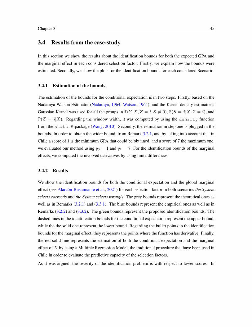
Chapter 3 45

3.4 Results from the case-study

In this section we show the results about the identification bounds for both the expected GPA and

the marginal effect in each considered selection factor. Firstly, we explain how the bounds were

estimated. Secondly, we show the plots for the identification bounds for each considered Scenario.

3.4.1 Estimation of the bounds

The estimation of the bounds for the conditional expectation is in two steps. Firstly, based on the

Nadaraya-Watson Estimator (Nadaraya, 1964; Watson, 1964), and the Kernel density estimator a

Gaussian Kernel was used for all the groups in E(Y |X,Z = i, S 6= 0),P(S = j|X,Z = i), and

P(Z = i|X). Regarding the window width, it was computed by using the density function

from the stats R-package (Wang, 2010). Secondly, the estimation in step one is plugged in the

bounds. In order to obtain the wider bound, from Remark 3.2.1, and by taking into account that in

Chile a score of 1 is the minimum GPA that could be obtained, and a score of 7 the maximum one,

we evaluated our method using y0 = 1 and y1 = 7. For the identification bounds of the marginal

effects, we computed the involved derivatives by using finite differences.

3.4.2 Results

We show the identification bounds for both the conditional expectation and the global marginal

effect (see Alarcon-Bustamante et al., 2021) for each selection factor in both scenarios the System

selects correctly and the System selects wrongly. The grey bounds represent the theoretical ones as

well as in Remarks (3.2.1) and (3.3.1). The blue bounds represent the empirical ones as well as in

Remarks (3.2.2) and (3.3.2). The green bounds represent the proposed identification bounds. The

dashed lines in the identification bounds for the conditional expectation represent the upper bound,

while the the solid one represent the lower bound. Regarding the bullet points in the identification

bounds for the marginal effect, they represents the points where the function has derivative. Finally,

the red-solid line represents the estimation of both the conditional expectation and the marginal

effect of X by using a Multiple Regression Model, the traditional procedure that have been used in

Chile in order to evaluate the predictive capacity of the selection factors.

As it was argued, the severity of the identification problem is with respect to lower scores. In

Chapter 3 46

fact, for lower scores in a selection factor, we find high probabilities of not being enrolled in a

program. When all the bounds coincide we say that we do not have non-enrolled students with

these scores (see identification bounds for both the conditional expectation and the marginal effect

of Mathematics, Language, Sciences, and HGPA score). However, for the Ranking score we can

see that the identification problem is for higher scores also, and therefore non-enrolled students

with the maximum Ranking score are not enrolled.

The System selects correctly

The identification bounds give us a range of all the plausible values of the evaluated function

if a researcher is ready to believe in the proposed identification restrictions. In this context, if

we are ready to believe that the score in the selection factor is the unique one that can predict

the performance in the GPA, to predict the GPA with the available information only is a plausible

solution for learning about the expected GPA, i.e., the regression E(Y |X,S 6= 0) under ignorability

is in between of the bounds in all the cases.

Regarding the marginal effect, we can see that if the Scenario 1 is considered (i.e., we assume that

selection factors are the unique predictor for the performance in the university, and the selection

factor is such that high scores will produce high performance) if non-enrolled students had enrolled,

a plausible scenario is that they were caused a null effect of the scores over the GPA. However, if

students with scores greater than 700 in mathematics test would be enrolled, the marginal effect

would be positive (see the identification bounds for the Global Marginal Effect in Figures 3.3a,

3.3d, and 3.3c).

By considering the interpretation of the marginal effect in partitioned populations provided in

Alarcon-Bustamante et al. (2021), we can see that if in the non-enrolled students the predictability

of the scores over the GPA is equal to the maximum one in each group, then the global marginal

effect of score in Mathematics, Sciences and HGPA score has a tendency of being a decreasing

function of the scores. Thus, if Scenario 1 holds, for lower score values, there is a larger proportion

of students belonging to a program where the marginal effect of Mathematics and Sciences test

score, and HGPA score is high. In contrast, for higher scores, a larger proportion of students will

be found for a program where the marginal effect is low. Regarding to the global marginal effect

of score in Language, and Ranking score, they have a tendency of being a constant function of the

Chapter 3 47

500 550 600 650 700 750 800 850

12

34

56

7

GPA

Score in Mathematics Test

500 550 600 650 700 750 800 850

−0.0

50.0

00.0

50.1

0

Glo

bal M

arg

inal E

ffect

Score in Mathematics Test

(a) Identification bounds in the Mathematics test

500 550 600 650 700 750 800 850

12

34

56

7

GPA

Score in Language Test

500 550 600 650 700 750 800 850

−0.0

50.0

00.0

50.1

0

Glo

bal M

arg

inal E

ffect

Score in Language Test

(b) Identification bounds in the Language and Com-

munication test

500 550 600 650 700 750 800 850

12

34

56

7

GPA

Score in Sciences Test

500 550 600 650 700 750 800 850

−0.0

50.0

00.0

50.1

0

Glo

bal M

arg

inal E

ffect

Score in Sciences Test

(c) Identification bounds in the Sciences test

550 600 650 700 750 800 850

12

34

56

7

GPA

HGPA score

500 550 600 650 700 750 800 850

−0.0

50.0

00.0

50.1

0

Glo

bal M

arg

inal E

ffect

HGPA score

(d) Identification bounds in HGPA selection factor

550 600 650 700 750 800 850

12

34

56

7

GPA

Ranking score

500 550 600 650 700 750 800 850

−0.0

50.0

00.0

50.1

0

Glo

bal M

arg

inal E

ffect

Ranking score

(e) Identification bounds in Ranking selection factor

Figure (3.3) Identification bounds for both the conditional expectation (left-side) and the

Marginal Effect (right-side) assuming that the System selects correctly.

scores. Thus, if Scenario 1 holds, for lower and upper score values, there is the same proportion

of students belonging to a program where the marginal effect of Language test score, and Ranking

score is high or low.

Note that the lower bound is near to be equal to the marginal effect when the traditional procedure

is used in Chile to evaluate the predictive capacity of the selection factors. Hence, if it assumed

Chapter 3 48

both that the scores of selection factors in non-enrolled students is zero and that Scenario 1 holds,

the enrolment of non-enrolled applicants would have produced a null global marginal effect for all

the selection factors.

The System selects wrongly

As it was mentioned before, assuming that the system selects wrongly, is analogous to assume that

the selection factors are not the unique ones that can predict the performance in the GPA. In this

context, we can think that if an applicant that was not-selected by the system had been selected,

its performance would be better than a selected one. This identification restriction allowed making

more informative the lower bound for both the conditional expectation and the marginal effect.

Regarding the first one, for all the selection factors the lower bound is practically equivalent to

the regression line under the ignorability assumption. Thus, if we are ready to believe that the

expected GPA, given the test scores, in non-enrolled applicants had been at least equal to the

ones in enrolled students we obtain that E(Y |X) ≈ E(Y |X,S 6= 0) (see the lower bound for

the conditional expectation in Figures 3.4a, 3.4b, and 3.4c). For the HGPA score, this fact is

reflected in scores higher than 600, and for the Ranking score, higher that 700. In this context, the

ignorability assumption could reflect that the system selects wrongly because a plausible solution

of the regression when this scenario is assumed (the lower bound) is equal to the regression under

ignorability.

Regarding the Global Marginal Effect, the lower bound in Mathematics and Science tests are higher

than the one when the using Multiple Regression Model is used for learning about the effect of

the selection factor scores over the GPA. Hence, if we assume that the impact of scores over the

GPA in the observed group, Z = i, S 6= 0, is at most equal to the one in the non-observed group,

Z = i, S = 0, the marginal effect using Multiple Regression Model is not a plausible solution.

Taking into account the interpretation of the Global Marginal Effect, we have that its tendency is

near to be constant, thus for lower or higher scores, we will find in the same proportion students in

both belonging to a program where the marginal effect is high and belonging to a program where

the marginal effect is low.

Chapter 3 49

500 550 600 650 700 750 800 850

12

34

56

7

GPA

Score in Mathematics Test

500 550 600 650 700 750 800 850

−0.0

50.0

00.0

50.1

0

Glo

bal M

arg

inal E

ffect

Score in Mathematics Test

(a) Identification bounds in Mathematics test

500 550 600 650 700 750 800 850

12

34

56

7

GPA

Score in Language Test

500 550 600 650 700 750 800 850

−0.0

50.0

00.0

50.1

0

Glo

bal M

arg

inal E

ffect

Score in Language Test

(b) Identification bounds in Language and Communi-

cation test

500 550 600 650 700 750 800 850

12

34

56

7

GPA

Score in Sciences Test

500 550 600 650 700 750 800 850

−0.0

50.0

00.0

50.1

0

Glo

bal M

arg

inal E

ffect

Score in Sciences Test

(c) Identification bounds in Sciences test

500 550 600 650 700 750 800 850

12

34

56

7

GPA

HGPA Score

500 550 600 650 700 750 800 850

−0.0

50.0

00.0

50.1

0

Glo

bal M

arg

inal E

ffect

HGPA Score

(d) Identification bounds in HGPA selection factor

500 550 600 650 700 750 800 850

12

34

56

7

GPA

Ranking Score

500 550 600 650 700 750 800 850

−0.0

40.0

00.0

40.0

8

Glo

bal M

arg

inal E

ffect

Ranking Score

(e) Identification bounds in Ranking selection factor

Figure (3.4) Identification bounds for both the conditional expectation (left-side) and the

Marginal Effect (right-side) assuming that the System selects wrongly.

3.5 Conclusions and discussion

We have used a partial identification approach for learning about both the conditional expectation

and the marginal effect of test scores over a variable of interest. From a modelling perspective,

we have generalised the Global Marginal Effect definition of Alarcon-Bustamante et al. (2021) to

Chapter 3 50

the case of partial observability of the outcome. This was carried out by making a partition of the

whole population of the applicants, and not assuming a prior distributional knowledge about the

missing GPAs. In fact, we considered not only the desired properties of a selection test but also

the possible Scenarios in the selection process in Chile. More specifically, we used monotonicity

assumptions in order to find the set of all the possible values of the marginal effect by considering

that the selection process is correct (or wrong). In this context, the main contribution of this chapter

is to show how a few ideas can help us to make inferences over the conditional expectation and its

derivative in presence of missing values.

Although the regression line, under the ignorability assumption is a plausible solution when Sce-

nario 1 is assumed, results illustrate that the current solution for learning about it is closer to reflect

that the system selects wrongly than the one selects correctly. Regarding the Marginal effect,

The low predictive capacity of the selection factors have caused multiple changes in the battery

tests in Chile (see DEMRE, 2016; Grassau, 1956; Donoso, 1998). Nevertheless, our results show

that assuming the only the proposed selection factors in Chile are useful to select is only a plausible

solution for learning about the predictive validity of the selection tests. Moreover, if other selection

factors were used, the predictive capacity of the tests would be maybe better.

Chapter 4

Final conclusions and remarks

“The credibility of inferences decreases with the strength of the assumptions maintained.”

Charles Manski: The Law of Decreasing Credibility.

Jerry Hausman, Professor of Economics at MIT in Cambridge, Massachusetts, USA, stated to

Charles Manski: you can not give the client a bound. The client needs a point. Nevertheless, point

predictions are produced by imposing strong assumptions that are rarely funded (Manski, 2013).

This work intends to propose how to draw conclusions based on both the problem and the pop-

ulation of interest. Although the used assumptions are not testable, they are weaker, and more

consistent, than the ones described in the introduction of this dissertation. Our interest was to de-

fine a new way to analyse the predictive validity of a selection test by considering all the available

information (about the applicants and the selected ones). Our partial identification methodology is

based on both a desired property of a selection test and the credibility about how the system selects.

This fact allows to interpret both the conditional expectation and the marginal effect according to

the credibility that a policy maker has about the chosen hypothesis.

Additionally to propose a new way to analyse and interpret a marginal effect for the case of

partitioned populations, we extended the idea of identification bounds for the effect of changes

in the explanartory random variable proposed by Manski (1989) to the case of multiple sampling

processes.

Even though the approach considered in this dissertation extended and tackled some drawbacks

of traditional strategies, there are some open questions to be discussed, which are listed bellow:

51

Chapter 4 52

1. This work make sense when exist a partial observability of the outcome only. Thus, we

assume that the covariates are fully observed. Nevertheless, in Chile there are elective tests,

and therefore some applicants take one and not the another. Thus, a relevant future work is

to consider different missing-data patterns and combine the results of Manski (2007) and the

ones of this dissertation.

2. A natural extension of this work is to consider the case where the conditional expectation

depends on more than one covariate.

3. In order to have a whole overview of the selection system in Chile, to generalise the partition

in Chapter 3 to more than three groups is considered as future work.

To finish this dissertation, we highlight that there is a not unique way to model a situation (e.g.,

by using the traditional distributional assumptions). In fact, we used assumptions related to the

problem that we intend to model. Finally, from our viewpoint, there is a necessity to make people

known how to deal with missing values and how stronger assumptions yield conclusions that are

more powerful but less credible (The Law of Decreasing Credibility Manski, 2003, p. 1).

Appendices

53

54

A Proof of the invariant property of the Global Marginal Effect

Proof. The global marginal effect in equation (2.2) is a function that depends on both X and Z,namely g(X,Z). Let z′ be any chosen reference group. Noting that pz′(X) = 1 −

∑z 6=z′

pz(X),

where pz(X) = P(Z = z|X) we have

g(X,Z = z′) =dE(Y |X,Z = z′)

dX+∑z 6=z′

[dE(Y |X,Z = z)

dX− dE(Y |X,Z = z′)

dX

]pz(X)

+∑z 6=z′

[E(Y |X,Z = z)− E(Y |X,Z = z′)]dpz(X)

dX

Now, suppose that another reference group, z′′ (z′ 6= z′′), is chosen. Then,

g(X,Z = z′′) =dE(Y |X,Z = z′′)

dX+∑z 6=z′′

[dE(Y |X,Z = z)

dX− dE(Y |X,Z = z′′)

dX

]pz(X)

+∑z 6=z′′

[E(Y |X,Z = z)− E(Y |X,Z = z′′)]dpz(X)

dX

By subtracting both functions we obtain

g(X,Z = z′)− g(X,Z = z′′) =

[dE(Y |X,Z = z′′)

dX− dE(Y |X,Z = z′)

dX

][∑z

pz(X)− 1

]

+ [E(Y |X,Z = z′′)− E(Y |X,Z = z′)]

d

[∑zpz(X)

]dX

Finally, because∑zpz(X) = 1, hence

[∑z

pz(X)− 1

]= 0 ;

d

[∑zpz(X)

]dX

= 0

This fact implies that

g(X,Z = z′)− g(X,Z = z′′) = 0,

and therefore g(X,Z = z′) = g(X,Z = z′′), for all z′ 6= z′′.

Remark A.1. Analogously, it can be proven that g(X,Z) is invariant under the chosen reference

group when Z ⊥⊥ X .

55

B Proof Proposition 3.2.1

Proof. Let us suppose that y0ix ≤ E(Y |X = x, Z = i, S = 0) ≤ y1ix, with y0ix ≤ y1ix.

Multiplying this inequality by P(S = 0, Z = i|X = x), we obtain that

y0ixP(S = 0, Z = i|X = x) ≤ E(Y |X = x, Z = i, S = 0)P(S = 0, Z = i|X = x) ≤

y1ixP(S = 0, Z = i|X = x).

Adding the term3∑j=1

E(Y |X = x, Z = i, S = j)P(S = j, Z = i|X = x) to this inequality, we

obtain that:

7∑i=1

y0ixP(Z = i|X = x, S = 0)P(S = 0|X = x) +

7∑i=1

3∑j=1

Eji(x)pji(x) ≤ E(Y |X = x)

≤7∑i=1

y1ixP(Z = i|X = x, S = 0)P(S = 0|X = x) +7∑i=1

3∑j=1

Eji(x)pji(x).

Provided that7∑i=1

P(Z = i|X = x, S = 0) = 1, and that we defined Y0x = (y01x, · · · , y07x), and

Y1x = (y11x, · · · , y17x) we have that

• E(Y0x|X = x, S = 0) =7∑i=1

y0ixP(Z = i|X = x, S = 0), and

• E(Y1x|X = x, S = 0) =7∑i=1

y1ixP(Z = i|X = x, S = 0)

56

C Proof Proposition 3.3.1

Let d+λ(X)dX

∣∣∣X=x

and d−λ(X)dX

∣∣∣X=x

be the positive and negative part of dλ(X)dX

∣∣∣X=x

respectively,

such that:

d+λ(X)

dX

∣∣∣∣X=x

= max

{0,dλ(X)

dX

∣∣∣∣X=x

}=

dλ(X)dX

∣∣∣X=x

if dλ(X)dX

∣∣∣X=x

> 0

0 otherwise,

and

d−λ(X)

dX

∣∣∣∣X=x

= max

{0,− dλ(X)

dX

∣∣∣∣X=x

}=

−dλ(X)

dX

∣∣∣X=x

if dλ(X)dX

∣∣∣X=x

< 0

0 otherwise.

Where dλ(X)dX

∣∣∣X=x

= d+λ(X)dX

∣∣∣X=x− d−λ(X)

dX

∣∣∣X=x

, and∣∣∣ dλ(X)

dX

∣∣∣X=x

∣∣∣ = d+λ(X)dX

∣∣∣X=x

+ d−λ(X)dX

∣∣∣X=x

.

Proof. Equation (3.5) can be written as:

MEX =

7∑i=1

[dE(Y |X,Z = i, S = 0)

dXP(S = 0|X,Z = i)

]P(Z = i|X)

+

7∑i=1

[3∑

j=1

[E(Y |X,Z = i, S = j)− E(Y |X,Z = i, S = 0)]dP(S = j|X,Z = i)

dX

]P(Z = i|X)

+

7∑i=1

E(Y |X,Z = i, S = 0)P(S = 0|X,Z = i)dP(Z = i|X)

dX

+

7∑i=1

[3∑

j=1

dE(Y |X,Z = i, S = j)

dXP(S = j|X,Z = i)

]P(Z = i|X)

+

7∑i=1

[3∑

j=1

E(Y |X,Z = i, S = j)P(S = j|X,Z = i)

]dP(Z = i|X)

dX. (1)

Because of both E(Y |X,Z = i, S = 0) and its derivative are not identified by data generating

process, the first three sums in (1) are not identified.

Let us suppose that D0ix ≤ dE(Y |X,Z=i,S=0)dX ≤ D1ix, thus for each X = x the first sum is

57

bounded as follows:

7∑i=1

D0ixP(S = 0|X = x, Z = i)P(Z = i|X = x) ≤

7∑i=1

[dE(Y |X,Z = i, S = 0)

dX

∣∣∣∣X=x

P(S = 0|X = x, Z = i)

]P(Z = i|X = x) ≤

7∑i=1

D1ixP(S = 0|X = x, Z = i)P(Z = i|X = x),

which it can be written as

[7∑i=1

D0ixP(Z = i|X = x, S = 0)

]P(S = 0|X = x) ≤

7∑i=1

[dE(Y |X,Z = i, S = 0)

dX

∣∣∣∣X=x

P(S = 0|X = x, Z = i)

]P(Z = i|X = x) ≤[

7∑i=1

D1ixP(Z = i|X = x, S = 0)

]P(S = 0|X = x),

Provided that7∑i=1

P(Z = i|X = x, S = 0) = 1, we have that:

E(D0x|X = x,S = 0)P(S = 0|X = x) ≤7∑i=1

[dE(Y |X,Z = i, S = 0)

dX

∣∣∣∣X=x

P(S = 0|X = x, Z = i)

]P(Z = i|X = x) ≤

E(D1x|X = x, S = 0)P(S = 0|X = x), (2)

Suppose that the non-observed conditional expectation is bounded by y0ix ≤ E(Y |X,Z = i, S =

0) ≤ y1ix. Thus, for each X = x, the identification region for the positive part of

3∑j=1

[E(Y |X = x, Z = i, S = j)− E(Y |X = x, Z = i, S = 0)]dP(S = j|X,Z = i)

dX

∣∣∣∣X=x

is bounded by

58

3∑j=1

[E(Y | X = x, Z = i, S = j)− y1ix]

d+P(S = j|X,Z = i)

dX

∣∣∣∣X=x

≤

3∑j=1

[E(Y |X = x, Z = i, S = j)− E(Y |X = x, Z = i, S = 0)]d+P(S = j|X,Z = i)

dX

∣∣∣∣X=x

≤

3∑j=1

[E(Y |X = x, Z = i, S = j)− y0ix]d+P(S = j|X,Z = i)

dX

∣∣∣∣X=x

. (3)

Analogously, the negative one is bounded by:

3∑j=1

[E(Y | X = x, Z = i, S = j)− y1ix]

d−P(S = j|X,Z = i)

dX

∣∣∣∣X=x

≤

3∑j=1

[E(Y |X = x, Z = i, S = j)− E(Y |X = x, Z = i, S = 0)]d−P(S = j|X,Z = i)

dX

∣∣∣∣X=x

≤

3∑j=1

[E(Y |X = x, Z = i, S = j)− y0ix]d−P(S = j|X,Z = i)

dX

∣∣∣∣X=x

. (4)

By subtracting (4) from (3), we obtain that

f+1i(x)− f−0i(x) ≤3∑

j=1

[E(Y |X = x, Z = i, S = j)− E(Y |X = x, Z = i, S = 0)]dP(S = j|X,Z = i)

dX

∣∣∣∣X=x

≤

f+0i(x)− f−1i(x)

Provided that7∑i=1

P(Z = i|X = x) = 1, we have that:

E(f+1 (X)− f−0 (X)|X = x) ≤7∑

i=i

3∑

j=1

[E(Y |X = x, Z = i, S = j)− E(Y |X = x, Z = i, S = 0)]dP(S = j|X,Z = i)

dX

∣∣∣∣X=x

× P(Z = i|X = x) ≤ E(f+0 (X)− f−1 (X)|X = x). (5)

59

Analogously to the previous identification bound, for each X = x, the positive part of

7∑i=1

E(Y |X,Z = i, S = 0)P(S = 0|X,Z = i)dP(Z = i|X)

dX

is bounded as follows:

7∑i=1

y0ixd+P(Z = i|X)

dX

∣∣∣∣X=x

P(S = 0|X = x, Z = i) ≤

7∑i=1

E(Y |X = x, Z = i, S = 0)P(S = 0|X = x, Z = i)d+P(Z = i|X)

dX

∣∣∣∣X=x

≤

7∑i=1

y1ixd+P(Z = i|X)

dX

∣∣∣∣X=x

P(S = 0|X = x, Z = i), (6)

and the negative one is bounded by

7∑i=1

y0ixd−P(Z = i|X)

dX

∣∣∣∣X=x

P(S = 0|X = x, Z = i) ≤

7∑i=1

E(Y |X = x, Z = i, S = 0)P(S = 0|X = x, Z = i)d−P(Z = i|X)

dX

∣∣∣∣X=x

≤

7∑i=1

y1ixd−P(Z = i|X)

dX

∣∣∣∣X=x

P(S = 0|X = x, Z = i). (7)

By subtracting (7) from (6) we obtain that

7∑i=1

[g+0i(x)−g−1i(x)]P(S = 0|X = x, Z = i) ≤

7∑i=1

E(Y |X = x, Z = i, S = 0)P(S = 0|X = x, Z = i)dP(Z = i|X)

dX

∣∣∣∣X=x

≤

7∑i=1

[g+1i(x)− g−0i(x)]P(S = 0|X = x, Z = i). (8)

Finally, if to the sum of (2), (5), and (8), the identified part of (1) is added, the identification region

in Proposition 3.3.1 holds.

60

D Proof for the width, W (x), given in 3.7.

Proof. From Equation (3.6), we have that

W (x) = E(D1x −D1x|X = x, S = 0)P(S = 0|X = x)

+ E(f+0 (X)− f−1 (X)− (f+1 (X)− f−0 (X))|X = x)

+

7∑i=1

(g+1i(x)− g−0i(x)− (g+0i(x)− g−1i(x)))P (S = 0|X = x, Z = i), (9)

where

E(f+0 (X)−f−1 (X)−(f+1 (X)−f−0 (X))|X = x) =

7∑i=1

(f+0i(x)−f+1i(x)+f−0i(x)−f−1i(x))P(Z = i|X = x)

Note that, on the one hand

f+0i(x)− f+1i(x) =

3∑j=1

(E(Y |X = x, Z = i, S = j)− y0ix)d+P(S = j|X,Z = i)

dX

∣∣∣∣X=x

− (E(Y |X = x, Z = i, S = j)− y1ix)d+P(S = j|X,Z = i)

dX

∣∣∣∣X=x

=3∑j=1

(y1ix − y0ix)d+P(S = j|X,Z = i)

dX

∣∣∣∣X=x

,

and

f−0i(x)− f−1i(x) =3∑j=1

(E(Y |X = x, Z = i, S = j)− y0ix)d−P(S = j|X,Z = i)

dX

∣∣∣∣X=x

− (E(Y |X = x, Z = i, S = j)− y1ix)d−P(S = j|X,Z = i)

dX

∣∣∣∣X=x

=3∑j=1

(y1ix − y0ix)d−P(S = j|X,Z = i)

dX

∣∣∣∣X=x

,

hence

E(f+0 (X)− f−1 (X)− (f+

1 (X)− f−0 (X))|X = x) =

7∑i=1

(3∑

j=1

(y1ix − y0ix)

∣∣∣∣ dP(S = j|X,Z = i)

dX

∣∣∣∣X=x

∣∣∣∣)

×P(Z = i|X = x). (10)

61

On the other hand,

g+1i(x)− g+0i(x) = y1ixd+

dXP(Z = i|X)

∣∣∣∣X=x

− y0ixd+P(Z = i|X)

dX

∣∣∣∣X=x

= (y1ix − y0ix)d+P(Z = i|X)

dX

∣∣∣∣X=x

and

g−1i(x)− g−0i(x) = y1ixd−

dXP(Z = i|X)

∣∣∣∣X=x

− y0ixd−

dXP(Z = i|X)

∣∣∣∣X=x

= (y1ix − y0ix)d−

dXP(Z = i|X)

∣∣∣∣X=x

.

Thus,

7∑i=1

(g+1i(x)− g−0i(x)− (g+0i(x)− g−1i(x)))P (S = 0|X = x, Z = i) =

7∑i=1

((y1ix − y0ix)

∣∣∣∣ dP(Z = i|X)

dX

∣∣∣∣X=x

∣∣∣∣)×P (S = 0|X = x, Z = i). (11)

Applying both (10) and (11) in (9), we have that

W (x) = E(D1x −D1x|X = x, S = 0)P(S = 0|X = x)

+

7∑i=1

3∑j=1

(y1ix − y0ix)

∣∣∣∣ dP(S = j|X,Z = i)

dX

∣∣∣∣X=x

∣∣∣∣P(Z = i|X = x)

+

7∑i=1

((y1ix − y0ix)

∣∣∣∣ dP(Z = i|X)

dX

∣∣∣∣X=x

∣∣∣∣)P (S = 0|X = x, Z = i)

= E(D1x −D0x|X = x, S = 0)P(S = 0|X = x)

+

7∑i=1

(yix − y0ix)

[∣∣∣∣ dP(Z = i|X)

dX

∣∣∣∣X=x

∣∣∣∣P(S = 0|X,Z = i)

+

3∑j=1

∣∣∣∣ dP(S = j|X,Z = i)

dX

∣∣∣∣X=x

∣∣∣∣P(Z = i|X = x)

Bibliography

Ai, C. and E. C. Norton (2003). Interaction terms in logit and probit models. Economic Letters 80,

123–129.

Alarcon-Bustamante, E., E. San Martın, and J. Gonzalez (2020). Predictive validity under partial

observability. In M. Wiberg, D. Molenaar, J. Gonzalez, U. Bockenholt, and J.-S. Kim (Eds.),

Quantitative Psychology, Cham, pp. 135–145. Springer International Publishing.

Alarcon-Bustamante, E., E. San Martın, and J. Gonzalez (2021). On the marginal effect under

partitioned populations: Definition and interpretation. In M. Wiberg, D. Molenaar, J. Gonzalez,

U. Bockenholt, and J.-S. Kim (Eds.), Quantitative Psychology. Springer International Publish-

ing.

American Educational Research Association, American Psychological Association, National

Council on Measurement in Education, and Joint Committee on Standards for Educational and

Psychological Testing (U.S) (2014). Standards for educational and psychological testing. Wash-

ington, DC : American Educational Research Association.

Ayers, J. B. and M. Peters (1977). Predictive validity of the test of english as foreign language for

asian graduate students in engineering, chemistry, or mathematics. Educational and Psycholog-

ical Measurement (37), 461–46.

Beck, A., C. Ward, M. Mendelson, J. Mock, and J. Erbaugh (1961). An Inventory for Measuring

Depression. JAMA Psychiatry 4(6), 561–571.

Berry, D., M. Bosh, and A. Sund (2013). The role of range restriction and criterion contamination

in assessing differential validity by race/ethnicity. Journal of Business and Psychology 28(3),

345–359.

62

63

Bliss, C. I. (1934). The method of probits. Science 79(2037), 38–39.

Blyth, C. (1972). On Simpson’s Paradox and the Sure-Thing Principle. Journal of the American

Statistical Association 67(338), 364–366.

Cameron, A. and P. Trivedi (2005). Microeconometrics. Methods and Applications. Cambridge

University Press, New York.

Centro de Estudios, MINEDUC (2019). ¿que sabemos sobre admision a la educacion superior? una

revision para implementacion del nuevo sistema de acceso en chile. santiago, chile. Technical

report, Ministerio de Educacion.

Cornelissen, T. (2005). Standard errors of marginal effects in the heteroskedastic probit model.

Discussion paper.

DEMRE (2016, 9). Prueba de seleccion universitaria. Technical report, Universidad de Chile.

Donoso, S. (1998). La reforma educacional y el sistema de seleccion de alumnos a las universi-

dades: impactos y cambios demandados. Estudios Pedagogicos (24), 7–30.

Florens, J. and M. Mouchart (1982). A note on noncausality. Econometrica 50(3), 583–592.

Geiser, S. and R. Studley (2002). UC and the SAT: Predictive Validity and Differential Impact of

the SAT I and SAT II at the University of California. Educational Assessment 8(1), 1–26.

Goldhaber, D., J. Cowan, and R. Theobald (2017). Evaluating Prospective Teachers: Testing the

Predictive Validity of the edTPA. Journal of Teacher Education 68(4), 377–393.

Grassau, E. (1956). Analisis estadıstico de las pruebas de bachillerato. Anales de la Universidad

de Chile (102), 77–93.

Green, K., G. Brown, S. Jager-Hyman, J. Cha, R. Steer, and A. Beck (2015). The Predictive Va-

lidity of the Beck Depression Inventory Suicide Item. The Journal of clinical psychiatry 76(12),

1683 – 1686.

Greene, W. H. (2003). Econometric analysis (5 ed.). Upper Saddle River, NJ: Prentice Hall.

64

Grobelny, J. (2018). Predictive Validity toward Job Performance of General and Specific Mental

Abilities. A Validity Study across Different Occupational Groups. Business and Management

Studies 4(3), 1–12.

GU, N. Y., Y. GAI, and J. W. HAY (2008). The effect of patient satisfaction with pharmacist

consultation on medication adherence: an instrumental variable approach. Pharmacy Pract

(Granada) 6(4), 201–210.

Guilliksen, H. (1950). Theory of mental tests. New York, John Willey and Sons.

Hayfield, T. and J. S. Racine (2008). Nonparametric econometrics: The np package. Journal of

Statistical Software 27(5).

Heckman, J. (1976). The common structure of statistical models of truncation, sample selection

and limited dependent variables and a simple estimator for such models. The Annals of Economic

and Social Measurement 46, 931–961.

Heckman, J. (1979). Sample selection bias as a specification error. Econometrica 47(1), 153–161.

Hirano, K. and G. W. Imbens (2004). The propensity score with continuous treatments. In

W. A. Shewhart and S. S. Wilks (Eds.), Applied Bayesian Modeling and Causal Inference from

Incomplete-Data Perspectives: An Essential Journey with Donald Rubin’s Statistical Family,

Chapter 7, pp. 73–84. Wiley Series in Probability and Statistics.

Imbens, G. (2000). The role of the propensity score in estimating dose-response functions.

Biometrika 87(3), 706–710.

Kennet-Cohen, T., S. Bronner, and C. Oren (1999). The predictive validity of the components of the

process of selection of candidates for higher education in Israel. National Institute for Testing

& evaluation.

Kobrin, J. L., Y. Kim, and P. R. Sackett (2012). Modeling the Predictive Validity of SAT Math-

ematics Items Using Item Characteristics. Educational and Psychological Measurement 72(1),

99–119.

Kolmogorov, A. N. (1950). Foundations of the theory of probability. New York: Chelsea Pub. Co.

65

Lawley, D. (1943). IV.-A note on Karl Pearson’s selection formulae. Proceedings of the Royal

Society of Edinburgh. Section A. Mathematical and Physical Science 62(1), 28–30.

Leong, C.-H. (2007). Predictive validity of the Multicultural Personality Questionnaire: A longi-

tudinal study on the socio-psychological adaptation of Asian undergraduates who took part in a

study-abroad program. International Journal of Intercultural Relations 31, 545–559.

Long, J. S. and S. A. Mustillo (2018). Using predictions and marginal effects to compare groups

in regression models for binary outcomes. Sociological Methods & Research, 1–37.

Lord, F. (1980). Applications of Item Response Theory To Practical Testing Problems. New York:

Routledge.

Makransky, G., P. Havmose, M. L. Vang, T. E. Andersen, and T. Nielsen (2017). The predictive

validity of using admissions testing and multiple mini-interviews in undergraduate university

admissions. Higher Education Research & Development 36(5), 1003–1016.

Manski, C. (1989). Anatomy of the selection problem. The Journal of Human Resources 24(3),

343–360.

Manski, C. (1993). Identification problems in the social sciences. Sociological Methodology 23,

1–56.

Manski, C. (2003). Partial Identification of Probability Distributions. New York: Springer.

Manski, C. (2005). Social Choice with Partial Knowledge of Treatment Response (1 ed.). New

Jersy: Princeton University Press.

Manski, C. (2007). Identification for Prediction and Decision. Harvard University Press.

Manski, C. (2013). Public Policy in an Uncertain World: Analysis and Decisions. Harvard Uni-

versity Press.

Manzi, J., D. Bravo, G. del Pino, G. Donoso, M. Martınez, and R. Pizarro (2008, 7). Estudio

de la validez predictiva de los factores de seleccion a las universidades del consejo de rectores,

admisiones 2003 al 2006. Technical report, Comite Tecnico Asesor, Honorable Consejo de

Rectores de las Universidades Chilenas.

66

Marchenko, Y. V. and M. G. Genton (2012). A Heckman Selection-t Model. Journal of the Amer-

ican Statistical Association 107(497), 304–317.

Meagher, D. G., A. Lin, and C. P. Stellato (2006). A predictive validity study of the pharmacy

college admission test. American journal of pharmaceutical education 70(3), 53.

Mendoza, J. and M. Mumford (1987). Corrections for attenuation and range restriction on the

predictor. Journal of Educational Statistics 12(3), 282–293.

Miller, R. and H. Frech (2000). Is there a link between pharmaceutical consumption and improved

health in oecd countries? Pharmacoeconomics 18(1), 33–45.

Nadaraya, E. (1964). On estimating regression. Theory of Probability and Its Applications 9(1),

141–2.

Nawata, K. (1994). Estimation of sample selection bias models by the maximum likelihood esti-

mator and Heckman’s two-step estimator. Economics Letters 45(1), 33–40.

Norton, E. C., H. Wang, and C. Ai (2004). Computing interaction effects and standrard errors in

logit and probit models. The stata journal 4(2), 154–167.

Pearson, K. (1903). Mathematical contribution to the theory of evolution-XI on the influence of

natural selection on the variability and correlation of organs. Philosophical Transactions of the

Royal Society of London 200(Ser. A), 1–66.

Powers, D. A. and Y. Xie (1999). Statistical Methods for Categorical Data Analysis. Academic

Press, Inc.

Simpson, E. (1951). The Interpretation of Interaction in Contingency Tables. Journal of the Royal

Statistical Society, Series B 13(2), 238–241.

Technical Advisory Committee, . (2010, 11). Resultados de la aplicacion de pruebas de seleccion

universitaria admisiones 2006 - 2010. Technical report, Consejo de Rectores Universidades

Chilenas.

Thorndike, R. (1949). Personnel selection: Test and measurement techniques. New York: Wiley.

67

Toomet, O. and A. Henningsen (2008). Sample selection models in R: Package sampleSelection.

Journal of Statistical Software 27(7).

Vasiljeva, M., I. Neskorodieva, V. Ponkratov, N. Kuznetsov, V. Ivlev, M. Ivleva, M. Maramygin,

and A. Zekiy (2020). A predictive model for assessing the impact of the covid-19 pandemic on

the economies of some eastern european countries. Journal of Open Innovation: Technology,

Market, and Complexity 6(3).

Wang, X.-F. (2010). fANCOVA: Nonparametric Analysis of Covariance. R package version 0.5-1.

Watson, G. (1964). Smooth regression analysis. Sankhya: The Indian Journal of Statistics, Series

A. 26(4), 359–372.

Wooldridge, J. M. (2010). Econometric analysis of cross section and panel data (2 ed.). Cambridge

MA: The MIT Press.

Wulff, J. N. (2014). Interpreting results from the multinomial logit model: Demonstrated by foreign

market entry. Organizational Research Methods 18(2), 1–26.