Noname manuscript No.

(will be inserted by the editor)

Modelling particulate self-healing materials and

application to uni-axial compression

Olaf Herbst · Stefan Luding

Received: June 9, 2008 / Accepted: date

Abstract Using an advanced history dependent contact model for DEM simulations,

including elasto-plasticity, viscosity, adhesion, and friction, pressure-sintered tablets

are formed from primary particles. These tablets are subjected to unconfined uni-

axial compression until and beyond failure. For fast and slow deformation we observe

ductile-like and brittle softening, respectively.

We propose a model for local self-healing that allows damage to heal during loading

such that the material strength of the sample increases and failure/softening is delayed

to larger strains. Local healing is achieved by increasing the (attractive) contact adhe-

sion forces for those particles involved in a potentially breaking contact.

We examine the dependence of the strength of the material on (a) the damage

detection sensitivity, (b) the damage detection rate, and (c) the (increased) adhesion

between healed contacts. The material strength is enhanced, i.e. the material fails at

larger strains and reaches larger maximal stress values, when any of the parameters (a)

– (c) is increased. For moderate damage detection sensitivities, the material strength

increases with both increasing healing rate and increasing adhesion of the healed con-

tacts. For very large adhesion between the healed contacts an interesting instability

with strong (brittle) fluctuations of the healed material’s strength is observed.

Keywords self-healing materials · granular materials · particle simulation · contact

force-laws · friction · adhesion · elasto-plastic contact deformation

PACS 45.70 · 47.50+d

O. Herbst and S. LudingMulti Scale Mechanics, TS, CTW, UTwente,P.O. Box 217, 7500 AE Enschede, The Netherlandse-mail: olaf.herbst@gmx.net, s.luding@utwente.nl

O. HerbstAerospace Engineering, TU Delft,Kluyverweg 1, 2629 HS Delft, The Netherlands,

2

1 Introduction

Self-healing materials encompass a wide range of materials capable of restoring their

functionality. They are inspired by healing mechanisms in biological systems [1]. For

example, the first healing of skin (or other tissues) results from coagulating blood.

Ideally, self-healing takes place locally at the damaged site and does not require an

(additional) external trigger. Applications of self-healing materials include the exten-

sion of service life of infrastructure or machinery [2]. In the future, advanced self-healing

capabilities may be crucial for the design and safety of new light-weight airplanes and

space applications [3,4].

Efforts to design such novel engineering materials able to heal cracks autonomously

have picked up considerably in recent years [5–7]. Intrinsic, self-activated healing has

been described in cement as early as 1918 [8] and a number of cementitious healing

mechanisms, both temporary and long lasting, have since been described, see, e.g.,

Refs. [9,10]. In recent years self healing properties have been incorporated into other

materials as well [11], often involving polymers. Functionality restoration has been

incorporated for crack healing inside the matrix of composite materials [6,12–19,3]

but also for, e.g., nano-coatings [20,21]. Advances have been achieved with respect

to designing a number of self-healing metal alloys, where diffusion is responsible for

self-healing, as well as for semiconductors [11].

In polymers self healing is usually achieved by the inclusion of a healing agent in

either microcapsules (see, e.g., Ref. [6], using a monomer), or hollow glass fibres [18,

3] filled with epoxy resin, and a catalyst, either spread out throughout the material

or in hollow glass fibres. When the material rips, microcapsules or rods can break

and release the healing agent. When the healing agent comes into contact with the

catalyst, it solidifies (in many cases through polimerization) restoring (part of) the

strength of the material. Polymers can achieve up to 100% of fracture strength after

healing, depending on the type of polymer, and the choice of self-healing agents [16].

Unfortunately, the introduction of a healing agent and catalyst into the material may

compromise the initial strength of the material. Other healing mechanisms include

the usage of non-covalent hydrogen bonds to control the polymer network [22]. While

some of the healing mechanisms require (exogeneous) heating [18], others are capable

of healing at ambient temperatures [6,15–17,23,24].

Efforts in designing self-healing cements have started much earlier [25–28]. In addi-

tion to methods similar to the ones used in polymers, i.e. using hollow fibres containing

superglue [5], many healing mechanisms are water-based [9]. These can be categorized

into two groups: autogeneous healing and hydration. The first group describes healing

mechanisms where the restored functionality persists in dry condition while the second

group describes systems that must remain saturated with water.

Computer based modelling of self-healing materials is not yet established. For solid

materials, most approaches can be categorized as either continuum approaches, e.g.

continuum damage models (CDM), or discrete element methods (DEM). The atomistic

molecular dynamics methods that have been used for, e.g., modelling crack growth [29]

shall only be mentioned here and not discussed further, since they typically describe

much smaller length-scales than both DEM or continuum methods.

While continuum approaches are extremely successful within their limits they re-

quire empirical constitutive relations for the material. They act on a coarse grained

level and the material must be (or is assumed to be) sufficiently homogeneous (or

“slowly changing”) on that coarse grained level. Continuum approaches therefore can

3

miss important details on smaller scales. For self healing materials almost all theo-

retical work is based on continuum approaches for different types of materials, see,

e.g., Refs. [30–32]. More specific examples for continuum models include a material

with nanoporous glass fibres containing glue [33], a memory alloy composite [34] or

nanoscale copper and biomaterial clusters [35]. Furthermore, a continuum model ap-

proach for a self healing material with enclosed capsules with glue as presented in 2001

by White and collaborators [6] has been published [36].

One way to simulate a material by means of particle simulations is to sinter a sam-

ple, e.g. a tablet, from primary particles to create a dense granular packing. Granular

materials are a very active field of research [37–47] and a natural toy model for ma-

terial science in general and self-healing materials in particular. Cohesive, frictional,

fine powders show a peculiar flow behavior [48–51]. Adhesionless powder flows freely,

but when adhesion due to van der Waals forces is strong enough, agglomerates or

clumps can form and break into pieces again [52–55]. This is enhanced by pressure- or

temperature-sintering [56] and, under extremely strong pressure, tablets or granulates

can be formed [57,58] from the primary particles.

Many-particle simulations like the discrete element model (DEM) [59–64] comple-

ment experiments on the scale of small “representative volume elements” (RVEs). They

allow deep and detailed insight into the kinematics and dynamics of the samples since

all information about all particles and contacts is available at all times. DEM requires

only the contact forces and torques as the basic input to solve the equations of motion

for all particles in such systems. Furthermore, the macroscopic material properties,

such as, among others, elastic moduli, cohesion, friction, yield strength, dilatancy, or

anisotropy can be measured from such RVE tests.

Research challenges involve not only realistic DEM simulations of many-particle

systems and their experimental validation, but also the transition from the microscopic

contact properties to the macroscopic behavior [50,51,64–66]. This so-called micro-

macro transition [50,51] should allow to better understand the collective flow behavior

of many particles as a function of their contact properties.

In a self healing model presented recently [58] the adhesion between all particles is

increased instantaneously at a given time (or strain) to simulate the healing (“global

healing”). While this may be a reasonable model for, e.g., healing through tempera-

ture induced sintering it is not a very realistic model for those kinds of self healing

materials, where, e.g., the breakage of microcapsules causes cracks to heal locally. For

this reason we present a simple model where healing is activated locally where and

when (potential) damage is detected. We examine the effect of the model parameters

(a) damage-detection sensitivity, (b) damage-detection rate, and (c) healing adhesion.

The paper is organized as follows. After introducing the simulation method in sec-

tion 2, the preparation of our samples is discussed in section 3. In section 4 we introduce

our self-healing model. In section 5 we discuss a self-healing material under compres-

sion. Summary and Conclusions are given in section 6 together with a discussion of the

relevance of our model for ”real” experiments and materials.

2 Discrete Particle Model

To simulate packing, failure under compression, and self-healing in a granular material

we use a Discrete Element Model (DEM) [57,59–63,67]. In the following we briefly

introduce the method that allows us to simulate self-healing solid materials as granular

4

packings. The numerics and algorithms are described in text books [68–70], so we only

discuss the basic input into DEM, i.e., the contact force models and parameters, see

Ref. [57] and references therein. We will, however, discuss in more detail the new self-

healing model based on the existing model.

Modelling inter-particle forces typically these forces are assumed to depend pairwise

on the overlap and the relative motion of two particles. This might not be sufficient

to account for the inhomogeneous stress distribution inside the particles and possible

multi-contact effects. However, this simplifying assumption makes it possible to study

larger samples of particles with a minimal complexity of the contact properties while

taking into account important phenomena like non-linear contact elasticity, plastic

deformation, and adhesion as well as friction.

2.1 Contact Force Laws

Realistic modeling of the deformations of only two particles in contact with each other

is quite challenging by itself. The description of many-body systems where each particle

can have multiple contacts is extremely complex. We therefore assume our particles

to be non-deformable perfect spheres which interact only when in contact. We call

two particles in contact when the distance of their centers of mass is less than the

sum of their radii. For two spherical particles i and j in contact, with radii ai and aj ,

respectively, we define their overlap

δ = (ai + aj) − (ri − rj) · n > 0 (1)

with the unit vector n := nij := (ri − rj)/|ri − rj | pointing from j to i. ri and rj

denote the position of paricle i and j, respectively.

The force f on particle i, labelled f i, is modelled to depend pairwise on all particles

with which particle i is in contact, f i =P

j f ci|j , where the sum runs over all particles

in contact with particle i and f ci|j is the force on particle i exerted by particle j

at contact. The force f ci|j can be decomposed into a normal and a tangential part,

f ci|j = fn

i|jn + f ti|jt, where n · t = 0. We will leave out the index i|j from now on. In

the following, we will first discuss the normal part of the force and then the tangential

part.

2.2 Normal Contact Forces

To model the normal componenent fn = fnel + fn

v of the force we use an adhesive,

elasto-plastic contact law that depends on three variables only and is described in

more detail in Ref. [57]: In this model the force between two spheres depends only on

their overlap δ, the relative velocity of their surfaces (including the relative normal and

tangential velocity, i.e. it depends on the translational and rotational velocities of the

two particles), and the maximum overlap δmax this contact has suffered in the past.

More specifically, we apply (a modificaton of) one of the simplest elasto-plastic

models: a modified spring-dashpot model. The dashpot is, as usual, a viscous damping

force that depends linearly on the normal component of the relative velocity (i.e. fnv =

γnδ). The force associated with the spring depends linearly on the overlap δ (i.e.

fnel = k∗δ) where, however, the stiffness “constant” k∗, itself depends on the history

5

c

*

δ

maxδ δ δδ* material

c,max

−kf

0f

k1δ

δ

f 2k fδ−δ( )

k δ−δ*( )

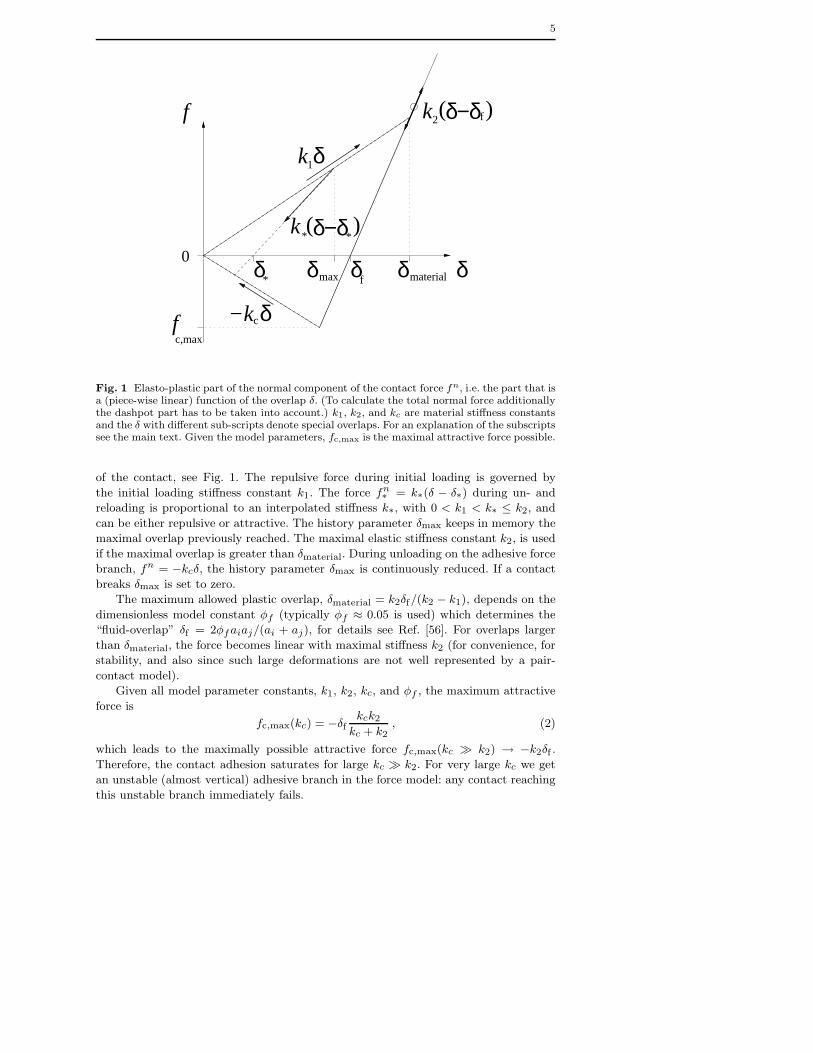
Fig. 1 Elasto-plastic part of the normal component of the contact force fn, i.e. the part that isa (piece-wise linear) function of the overlap δ. (To calculate the total normal force additionallythe dashpot part has to be taken into account.) k1, k2, and kc are material stiffness constantsand the δ with different sub-scripts denote special overlaps. For an explanation of the subscriptssee the main text. Given the model parameters, fc,max is the maximal attractive force possible.

of the contact, see Fig. 1. The repulsive force during initial loading is governed by

the initial loading stiffness constant k1. The force fn∗ = k∗(δ − δ∗) during un- and

reloading is proportional to an interpolated stiffness k∗, with 0 < k1 < k∗ ≤ k2, and

can be either repulsive or attractive. The history parameter δmax keeps in memory the

maximal overlap previously reached. The maximal elastic stiffness constant k2, is used

if the maximal overlap is greater than δmaterial. During unloading on the adhesive force

branch, fn = −kcδ, the history parameter δmax is continuously reduced. If a contact

breaks δmax is set to zero.

The maximum allowed plastic overlap, δmaterial = k2δf/(k2 − k1), depends on the

dimensionless model constant φf (typically φf ≈ 0.05 is used) which determines the

“fluid-overlap” δf = 2φfaiaj/(ai + aj), for details see Ref. [56]. For overlaps larger

than δmaterial, the force becomes linear with maximal stiffness k2 (for convenience, for

stability, and also since such large deformations are not well represented by a pair-

contact model).

Given all model parameter constants, k1, k2, kc, and φf , the maximum attractive

force is

fc,max(kc) = −δfkck2

kc + k2

, (2)

which leads to the maximally possible attractive force fc,max(kc ≫ k2) → −k2δf .

Therefore, the contact adhesion saturates for large kc ≫ k2. For very large kc we get

an unstable (almost vertical) adhesive branch in the force model: any contact reaching

this unstable branch immediately fails.

6

The motivation behind this model is to use the simplest model possible that is (at

least piecewise) linear (in order to allow some theoretical analysis) while keeping the

necessary phenomena such as plastic deformation, adhesion, and history dependence.

For example, when two particles have been plastically deformed during loading their

repulsive forces during unloading will be smaller than they were during loading and

the contact will be completely unloaded before it reaches zero overlap (measured in

terms of their original shape). When a real material is deformed it will memorize every

deformation and the corresponding path. This is an extremely complex process. We

simplify this complex process by keeping in memory only the maxium overlap a contact

has suffered in the past. This allows us to model elasticity, plastic deformation, and

adhesion to some extent. It does not represent all other possible complex mechanisms

at contacts of particles. In that respect our model is a compromise between “as simple

as possible” and “realistic enough” for our purposes.

2.3 Tangential Contact Forces

In the tangential direction, the forces and torques depend on the tangential displace-

ment and the relative rotations of the particle surfaces. Dynamic (sliding) and static

friction depend on the tangential component of the relative velocity of the contact

points,

vt = vij − n(n · vij) , where vij = vi − vj + a′in × ωi + a′jn × ωj (3)

is the relative velocity of the particle surfaces at contact. Here a′α = aα − δ/2, for

α = i, j, is the corrected radius relative to the contact point. vi, vj , ωi, and ωj are

the linear and rotational velocities of particles i and j, respectively.

Tangential forces f t acting on the contacts are modelled to be proportional to the

accumulated sliding distance of the contact points along each other with a (tangential)

stiffness constant kt, i.e. f t = kt

R

vtdt. Including also a viscous dependent damping

constant, γt, the tangential force is limited by the product of the normal force and the

contact friction coefficient µ, according to Coulombs law, f t ≤ µfn, for more details

see Ref. [57]. Note, however, that this commonly used tangential force model is rather

simple – leaving most of the complexity in the normal force model.

2.4 Background Viscous Damping

Viscous dissipation as mentioned above takes place localized in a two-particle contact

only. In the bulk material, where many particles are in contact with each other, this

dissipation mode is very inefficient for long-wavelength cooperative modes of motion,

especially when linear force laws are involved [71]. Therefore, an additional (artificial)

damping with the background is introduced, such that the total force f i and torque

qi|j := a′jn × f i|j on particle i are given by

f i =X

j

“

fnn + f t

t”

− γbvi and qi =X

j

qi|j − γbra2i ωi , (4)

where the sums take into account all contact partners j of particle i, and γb and γbr

are the (artificial) background damping viscosities assigned to the translational and

7

rotational degrees of freedom, respectively. The viscosities can be seen as originating

from a viscous inter-particle medium and enhance the damping in the spirit of a rapid

relaxation and equilibration. Note that the effect of γb and γbr should be checked for

each set of parameters: it should be small in order to rule out artificial over-damping.

2.5 Contact model Parameters

In the following we measure length in units of 1mm, mass in 1 mg and time in 1 µs.

Note that only a few parameters have to be specified with dimensions, while the others

are expressed as dimensionless ratios in table 1.

Property Symbol Value dimensional units SI-units

Time unit tu 1 1 µs 10−6 sLength unit xu 1 1mm 10−3 mMass unit mu 1 1mg 10−6 kgAverage article radius a0 0.005 5 µm 510−6mMaterial density ρ 2 2 mg/mm3 2000 kg/m3

Max. loading/unloading stiffness k2 5 5mg/µs2 5 106 kg/s2

Initial loading stiffness k1/k2 0.5Adhesion parameter kc/k2 0.2Tangential stiffness kt/k2 0.2Coulomb friction coefficient µ 1Normal viscosity γ = γn 5 10−5 5 10−5 mg/µs 5 101 kg/sFriction viscosity γt/γ 0.2Background viscosity γb/γ 4.0Background viscous torque γbr/γ 1.0Fluid overlap φf 0.05

Table 1 Values of the microscopic material parameters used (third column), if not explicitlyspecified. The fourth column contains these values in the appropriate units, i.e., when thetime-, length-, and mass-units are µs, mm, and mg, respectively. Column five contains theparameters in SI-units. Energy, force, acceleration, and stress have to be scaled with factorsof 1, 103, 109, and 109, respectively, for a transition from dimensionless to SI-units.

A maximal stiffness constant of k2 = 5, as used in our simulations, corresponds

to a typical contact duration (half-period) tc ≈ 6.5 × 10−4 for a typical collision

of a large and a small particle with γ = 0. Accordingly, an integration time-step of

tMD = 5 × 10−6 is used in order to allow for a “safe” integration of the equations of

motion. Note that not only the normal “eigenfrequency” but also the eigenfrequencies

for the rotational dedrees of freedom have to be considered as well as the viscous

response times tγ ≈ m/γ. All of the physical time scales (inverse eigenfrequencies)

should be considerably larger than tMD, while the viscous response times should be

even larger, such that tγ > tc > tMD. A more detailed discussion of all the effects due

to the interplay between the model parameters and the related times is, however, far

from the scope of this paper and can be found in Ref. [57].

8

3 Tablet preparation and material failure test

3.1 Tablet preparation

Having introduced the model and its parameters in the last section we describe now the

experimental setup and the basic steps of our simulations. First, a “tablet” (granule)

is prepared from primary particles which behave according to the contact force laws

described above. A four-step process is applied:

1. creation of a loose initial sample

2. pressure sintering by isotropic compression

3. removal of the pressure

4. relaxation

On the resulting “tablet”, or material sample, or RVE, tests can be performed, e.g.

controlled compression or tensile tests, both on the “plain” tablet as well as under

self-healing conditions. Care has to be taken to perform first the preparation and later

the tests in a symmetric way (see below) to avoid artefacts.

3.1.1 Initial sample

Before sintering the tablet the first step is to create a loose configuration of N = 1728

spherical particles with a Gaussian distribution of radii with average a0 = 0.005. The

tails of the distribution are cut off at 0.003 and 0.0075 to ensure that all particles

are comparable in size [72], i.e. neither too large nor too small particles are desired.

For the samples presented in this paper, the half-width of the distribution is wa =p

〈a2〉 − 〈a〉2 = 0.0007213. In addition, the initial velocities are drawn from a Gaussian

distribution in each direction.

In the initial preparation stage the particles are arranged on a regular cubic lattice

with wide spacing so that particles are not in contact – neither with each other nor

with a wall. Then, with µ = 0 and kc = 0 (i.e. zero friction and zero adhesion), the

system is compressed with a pressure of p1 = 0.5 to create a loose initial isotropic

packing with (after relaxation) a coordination number C = 5.89 and volume fraction,

ν =P

i V (ai)/V = 0.607, where V (ai) = (4/3)πa3i is the volume of one particle i.

3.1.2 Pressure sintering

The second step is pressure sintering: The system is compressed by keeping one wall

in each spatial direction fixed while applying a constant pressure of ps = 10 to the

other (three) walls. During this compression, the particles are frictional with a friction

coefficient µ = 1, and have zero adhesion amongst each other, i.e. kc = 0. Four of the

six walls are frictionless, µwall = 0, and cohesionless, kwallc = 0. The remaining two

(opposing) walls are already prepared for the tests to come: These two walls define the

uni-axial direction and are strongly adhesive, with kwallc /k2 = 20, such that the sample

sticks to them, while all other walls can be easily removed in the third step described

below. The wall adhesion has no visible effect here, since the sample is strongly confined.

In contrast, friction has an effect, i.e. friction with the walls would hinder the pressure

to be transferred completely to the opposite wall. Frictional walls carry part of the

load – an effect that is known since the early work of Janssen [73,74].

9

10-25

10-20

10-15

10-10

10-5

0.0001 0.001 0.01 0.1 1 10

Eki

n

t

5.8

6

6.2

6.4

6.6

6.8

7

7.2

7.4

0.0001 0.001 0.01 0.1 1 10

C

t

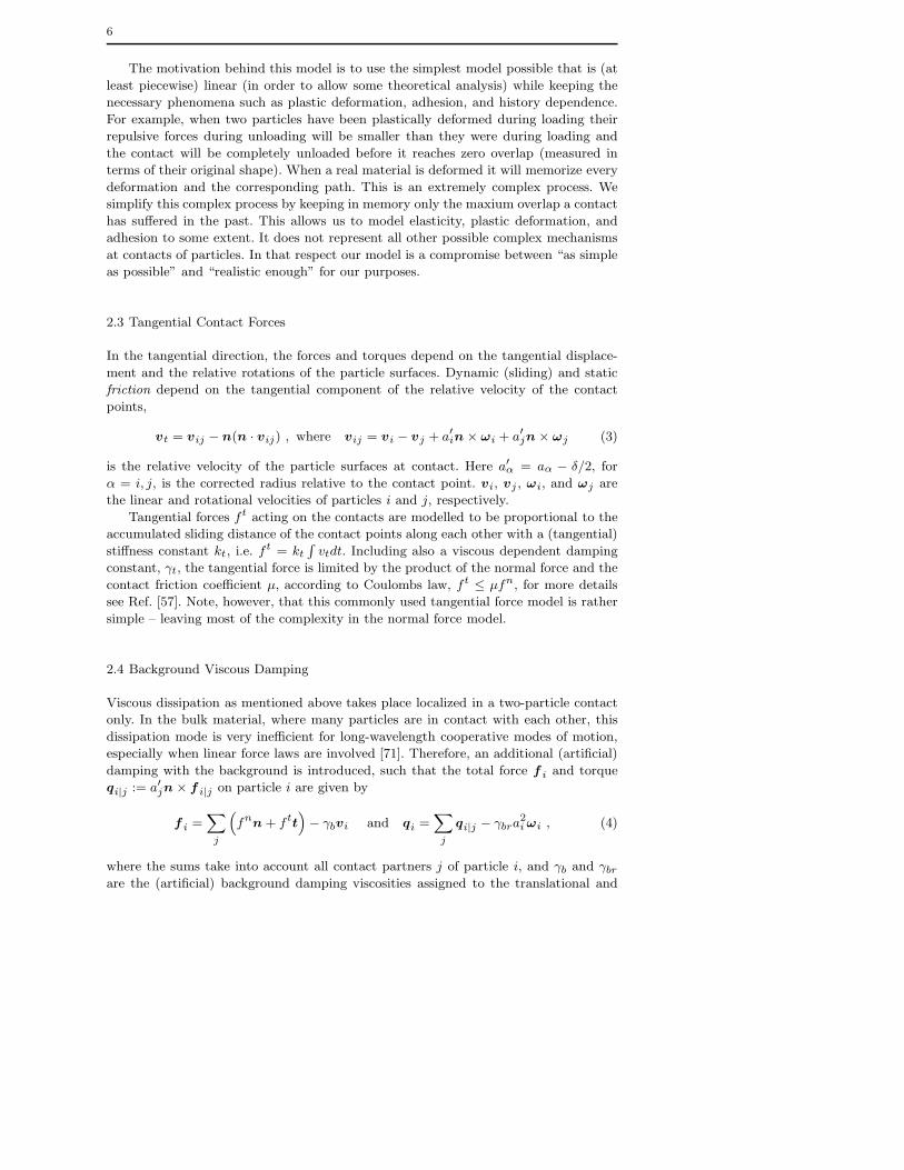
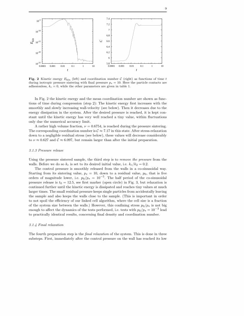
Fig. 2 Kinetic energy Ekin (left) and coordination number C (right) as functions of time tduring isotropic pressure sintering with final pressure ps = 10. Here the particle contacts areadhesionless, kc = 0, while the other parameters are given in table 1.

In Fig. 2 the kinetic energy and the mean coordination number are shown as func-

tions of time during compression (step 2): The kinetic energy first increases with the

smoothly and slowly increasing wall-velocity (see below). Then it decreases due to the

energy dissipation in the system. After the desired pressure is reached, it is kept con-

stant until the kinetic energy has very well reached a tiny value, within fluctuations

only due the numerical accuracy limit.

A rather high volume fraction, ν = 0.6754, is reached during the pressure sintering.

The corresponding coordination number is C ≈ 7.17 in this state. After stress-relaxation

down to a negligible residual stress (see below), these values will decrease considerably

to ν ≈ 0.627 and C ≈ 6.097, but remain larger than after the initial preparation.

3.1.3 Pressure release

Using the pressure sintered sample, the third step is to remove the pressure from the

walls. Before we do so kc is set to its desired initial value, i.e. kc/k2 = 0.2.

The control pressure is smoothly released from the walls in a co-sinusoidal way.

Starting from its sintering value, ps = 10, down to a residual value, p0, that is five

orders of magnitude lower, i.e. p0/ps = 10−5. The half period of the co-sinusoidal

pressure release is t0 = 12.5, see first marker (open circle) in Fig. 3, but relaxation is

continued further until the kinetic energy is dissipated and reaches tiny values at much

larger times. The small residual pressure keeps single particles from accidentally leaving

the sample and also keeps the walls close to the sample. (This is important in order

to not spoil the efficiency of our linked cell algorithm, where the cell size is a fraction

of the system size between the walls.) However, this confining stress p0/ps is not big

enough to affect the dynamics of the tests performed, i.e. tests with p0/ps = 10−3 lead

to practically identical results, concerning final density and coordination number.

3.1.4 Final relaxation

The fourth preparation step is the final relaxation of the system. This is done in three

substeps. First, immediately after the control pressure on the wall has reached its low

10

10-25

10-20

10-15

10-10

10-5

0.01 0.1 1 10 100

Eki

n

t

5.8

6

6.2

6.4

6.6

6.8

7

7.2

7.4

0.001 0.01 0.1 1 10 100

C

t

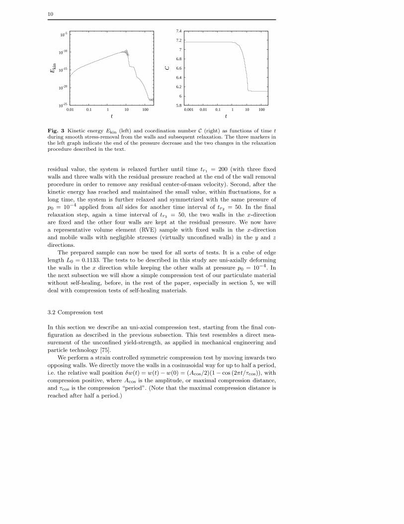
Fig. 3 Kinetic energy Ekin (left) and coordination number C (right) as functions of time tduring smooth stress-removal from the walls and subsequent relaxation. The three markers inthe left graph indicate the end of the pressure decrease and the two changes in the relaxationprocedure described in the text.

residual value, the system is relaxed further until time tr1= 200 (with three fixed

walls and three walls with the residual pressure reached at the end of the wall removal

procedure in order to remove any residual center-of-mass velocity). Second, after the

kinetic energy has reached and maintained the small value, within fluctuations, for a

long time, the system is further relaxed and symmetrized with the same pressure of

p0 = 10−4 applied from all sides for another time interval of tr2= 50. In the final

relaxation step, again a time interval of tr3= 50, the two walls in the x-direction

are fixed and the other four walls are kept at the residual pressure. We now have

a representative volume element (RVE) sample with fixed walls in the x-direction

and mobile walls with negligible stresses (virtually unconfined walls) in the y and z

directions.

The prepared sample can now be used for all sorts of tests. It is a cube of edge

length L0 = 0.1133. The tests to be described in this study are uni-axially deforming

the walls in the x direction while keeping the other walls at pressure p0 = 10−4. In

the next subsection we will show a simple compression test of our particulate material

without self-healing, before, in the rest of the paper, especially in section 5, we will

deal with compression tests of self-healing materials.

3.2 Compression test

In this section we describe an uni-axial compression test, starting from the final con-

figuration as described in the previous subsection. This test resembles a direct mea-

surement of the unconfined yield-strength, as applied in mechanical engineering and

particle technology [75].

We perform a strain controlled symmetric compression test by moving inwards two

opposing walls. We directly move the walls in a cosinusoidal way for up to half a period,

i.e. the relative wall position δw(t) = w(t) −w(0) = (Acos/2)(1 − cos (2πt/τcos)), with

compression positive, where Acos is the amplitude, or maximal compression distance,

and τcos is the compression “period”. (Note that the maximal compression distance is

reached after half a period.)

11

For a representative volume element (RVE) like our sample, we quantify the de-

formation in terms of the strain imposed from two sides ε(t) = 2δw(t)/L0, with the

maximum strain εcos = 2Acos/L0. The time-derivative of the strain leads to the (time-

dependent) compression rate R(t) := ∂ε/∂t = Rcos sin (2πt/τcos) with the maximum

compression rate Rcos = 2πεcosτ−1cos reached at a quarter-period.

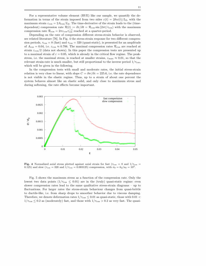
Depending on the rate of compression different stress-strain behavior is observed,

see related literature [76]. In Fig. 4 the stress-strain response for two different compres-

sion periods, τcos = 8 (fast) and τcos = 320 (quasi-static), is presented for an amplitude

of Acos = 0.04, i.e. εcos ≈ 0.706. The maximal compression rates Rcos are reached at

strain εcos/2 (data not shown). In this paper the compression tests are presented up

to a maximal strain of ε = 0.05, which is already in the critical flow regime. The peak-

stress, i.e. the maximal stress, is reached at smaller strains, εmax ≈ 0.01, so that the

relevant strain-rate is much smaller, but still proportional to the inverse period 1/τcos,

which will be given in the following.

In the compression tests with small and moderate rates, the initial stress-strain

relation is very close to linear, with slope C = ∂σ/∂ε = 225.6, i.e. the rate dependence

is not visible in the elastic regime. Thus, up to a strain of about one percent the

system behaves almost like an elastic solid, and only close to maximum stress and

during softening, the rate effects become important.

0

0.0005

0.001

0.0015

0.002

0.0025

0.003

0 0.01 0.02 0.03 0.04 0.05

σ / σ

0

ε

fast compressionslow compression

Fig. 4 Normalized axial stress plotted against axial strain for fast (τcos = 8 and 1/τcos =0.125) and slow (τcos = 320 and 1/τcos = 0.003125) compression, with σ0 = k2/a0 = 103.

Fig. 5 shows the maximum stress as a function of the compression rate. Only the

lowest two data points (1/τcos ≤ 0.01) are in the (truly) quasi-static regime: even

slower compression rates lead to the same qualitative stress-strain diagrams – up to

fluctuations. For larger rates the stress-strain behaviour changes from quasi-brittle

to ductile-like, i.e. from sharp drops to smoother behavior due to viscous damping.

Therefore, we denote deformation rates 1/τcos ≤ 0.01 as quasi-static, those with 0.01 <

1/τcos ≤ 0.2 as (moderately) fast, and those with 1/τcos > 0.2 as very fast. The quasi-

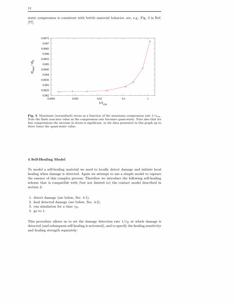
12

static compression is consistent with brittle material behavior, see, e.g., Fig. 3 in Ref.

[77].

0.002

0.0025

0.003

0.0035

0.004

0.0045

0.005

0.0055

0.006

0.0065

0.007

0.0075

0.0001 0.001 0.01 0.1 1

σ max

/ σ 0

1/τcos

Fig. 5 Maximum (normalized) stress as a function of the maximum compression rate 1/τcos.Note the finite non-zero value as the compression rate becomes quasi-static. Note also that forfast compressions the increase in stress is significant, in the data presented in this graph up tothree times the quasi-static value.

4 Self-Healing Model

To model a self-healing material we need to locally detect damage and initiate local

healing when damage is detected. Again we attempt to use a simple model to capture

the essence of this complex process. Therefore we introduce the following self-healing

scheme that is compatible with (but not limited to) the contact model described in

section 2:

1. detect damage (see below, Sec. 4.1),

2. heal detected damage (see below, Sec. 4.2),

3. run simulation for a time τD,

4. go to 1.

This procedure allows us to set the damage detection rate 1/τD at which damage is

detected (and subsequent self-healing is activated), and to specify the healing sensitivity

and healing strength separately:

13

0

k1δ

δ

f 2k

δ

δ−δ( )f

f

cα δcδ−k − k

x

x

x xx

xx

x

x

OO

OOO x

x

x x

x

xxx

xx

x

xx

x

x

xx xx

x

xx

xxx

x

xx

x

x

xx

xx

x

x x

x

x

x

xx

x

xx

xx

x

xx

x

xO

O OO

OO

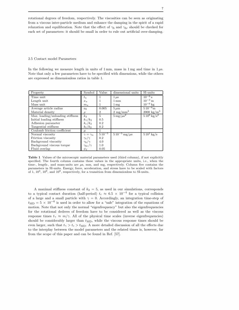
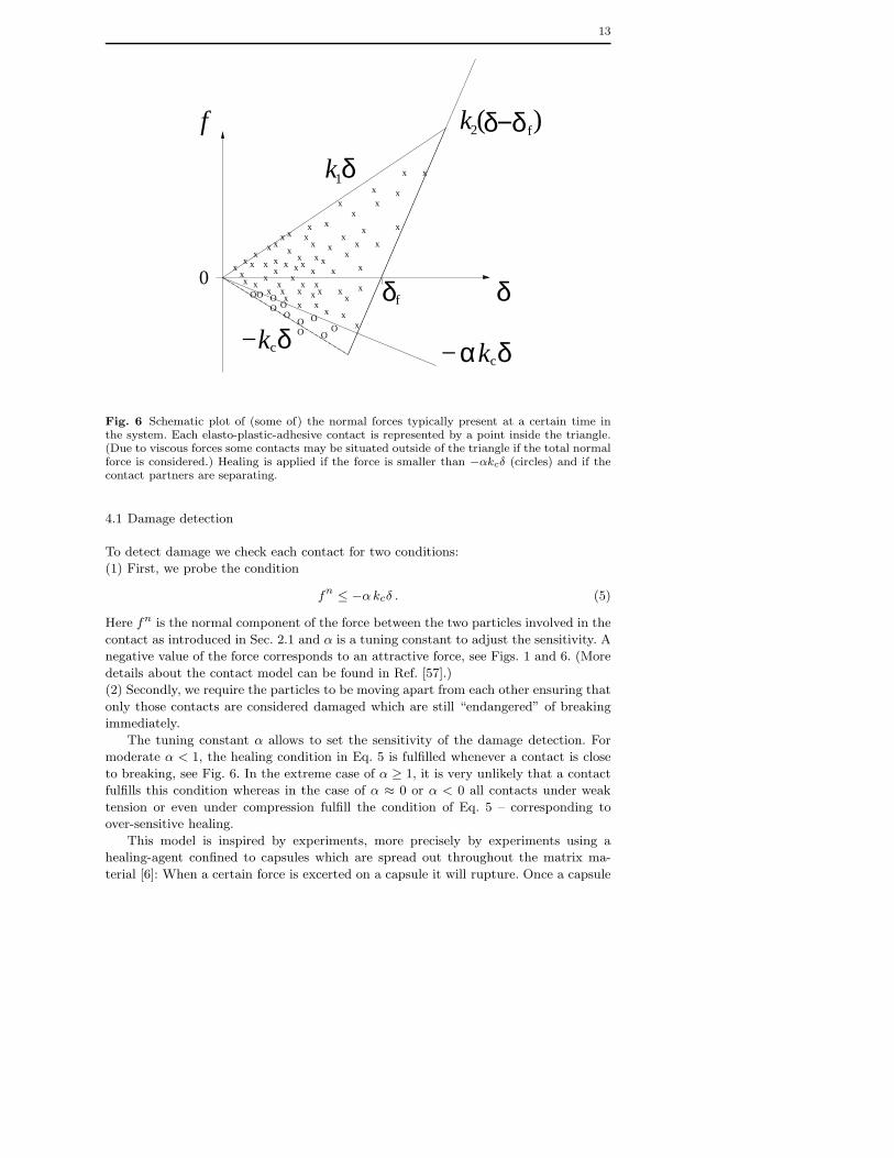
Fig. 6 Schematic plot of (some of) the normal forces typically present at a certain time inthe system. Each elasto-plastic-adhesive contact is represented by a point inside the triangle.(Due to viscous forces some contacts may be situated outside of the triangle if the total normalforce is considered.) Healing is applied if the force is smaller than −αkcδ (circles) and if thecontact partners are separating.

4.1 Damage detection

To detect damage we check each contact for two conditions:

(1) First, we probe the condition

fn ≤ −αkcδ . (5)

Here fn is the normal component of the force between the two particles involved in the

contact as introduced in Sec. 2.1 and α is a tuning constant to adjust the sensitivity. A

negative value of the force corresponds to an attractive force, see Figs. 1 and 6. (More

details about the contact model can be found in Ref. [57].)

(2) Secondly, we require the particles to be moving apart from each other ensuring that

only those contacts are considered damaged which are still “endangered” of breaking

immediately.

The tuning constant α allows to set the sensitivity of the damage detection. For

moderate α < 1, the healing condition in Eq. 5 is fulfilled whenever a contact is close

to breaking, see Fig. 6. In the extreme case of α ≥ 1, it is very unlikely that a contact

fulfills this condition whereas in the case of α ≈ 0 or α < 0 all contacts under weak

tension or even under compression fulfill the condition of Eq. 5 – corresponding to

over-sensitive healing.

This model is inspired by experiments, more precisely by experiments using a

healing-agent confined to capsules which are spread out throughout the matrix ma-

terial [6]: When a certain force is excerted on a capsule it will rupture. Once a capsule

14

is broken, the healing agent will flow out and solidify. After, there cannot be any further

healing at the same position again because there is no more healing agent available.

Different types of capsules and capsule-matrix interface can be modeled by different

healing sensitivities α. The present model does not allow for massive volume changes

(as due to foaming or bubbling healing agents).

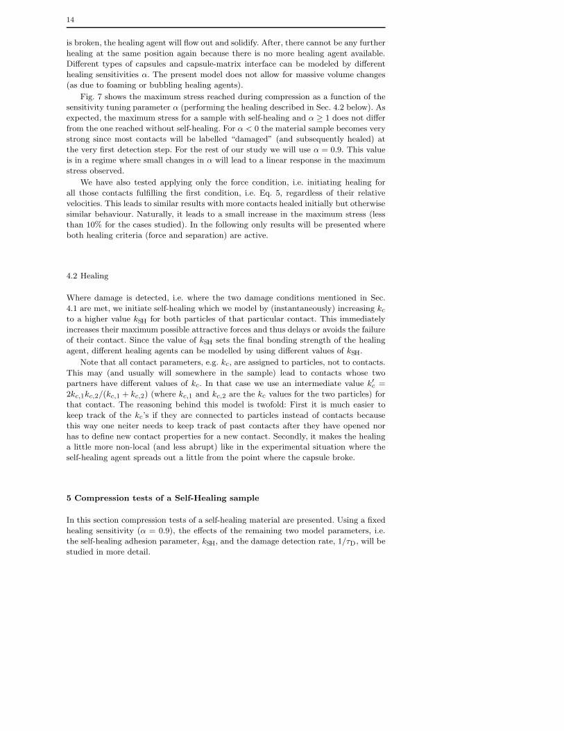
Fig. 7 shows the maximum stress reached during compression as a function of the

sensitivity tuning parameter α (performing the healing described in Sec. 4.2 below). As

expected, the maximum stress for a sample with self-healing and α ≥ 1 does not differ

from the one reached without self-healing. For α < 0 the material sample becomes very

strong since most contacts will be labelled “damaged” (and subsequently healed) at

the very first detection step. For the rest of our study we will use α = 0.9. This value

is in a regime where small changes in α will lead to a linear response in the maximum

stress observed.

We have also tested applying only the force condition, i.e. initiating healing for

all those contacts fulfilling the first condition, i.e. Eq. 5, regardless of their relative

velocities. This leads to similar results with more contacts healed initially but otherwise

similar behaviour. Naturally, it leads to a small increase in the maximum stress (less

than 10% for the cases studied). In the following only results will be presented where

both healing criteria (force and separation) are active.

4.2 Healing

Where damage is detected, i.e. where the two damage conditions mentioned in Sec.

4.1 are met, we initiate self-healing which we model by (instantaneously) increasing kc

to a higher value kSH for both particles of that particular contact. This immediately

increases their maximum possible attractive forces and thus delays or avoids the failure

of their contact. Since the value of kSH sets the final bonding strength of the healing

agent, different healing agents can be modelled by using different values of kSH.

Note that all contact parameters, e.g. kc, are assigned to particles, not to contacts.

This may (and usually will somewhere in the sample) lead to contacts whose two

partners have different values of kc. In that case we use an intermediate value k′c =

2kc,1kc,2/(kc,1 + kc,2) (where kc,1 and kc,2 are the kc values for the two particles) for

that contact. The reasoning behind this model is twofold: First it is much easier to

keep track of the kc’s if they are connected to particles instead of contacts because

this way one neiter needs to keep track of past contacts after they have opened nor

has to define new contact properties for a new contact. Secondly, it makes the healing

a little more non-local (and less abrupt) like in the experimental situation where the

self-healing agent spreads out a little from the point where the capsule broke.

5 Compression tests of a Self-Healing sample

In this section compression tests of a self-healing material are presented. Using a fixed

healing sensitivity (α = 0.9), the effects of the remaining two model parameters, i.e.

the self-healing adhesion parameter, kSH, and the damage detection rate, 1/τD, will be

studied in more detail.

15

0.0025

0.003

0.0035

0.004

0.0045

0.005

0.0055

0.006

0.0065

-0.2 0 0.2 0.4 0.6 0.8 1 1.2

σ max

/ σ 0

α

Fig. 7 Dependence of the maximum (normalized) stress reached by healing with differentsensitivities α, for the self-healing adhesion parameter kSH = 5 and damage detection rate1/τD = 0.002, while otherwise the same parameters as for Fig. 4 (moderately fast) were used.The horizontal line shows the maximum strength for a sample without self healing.

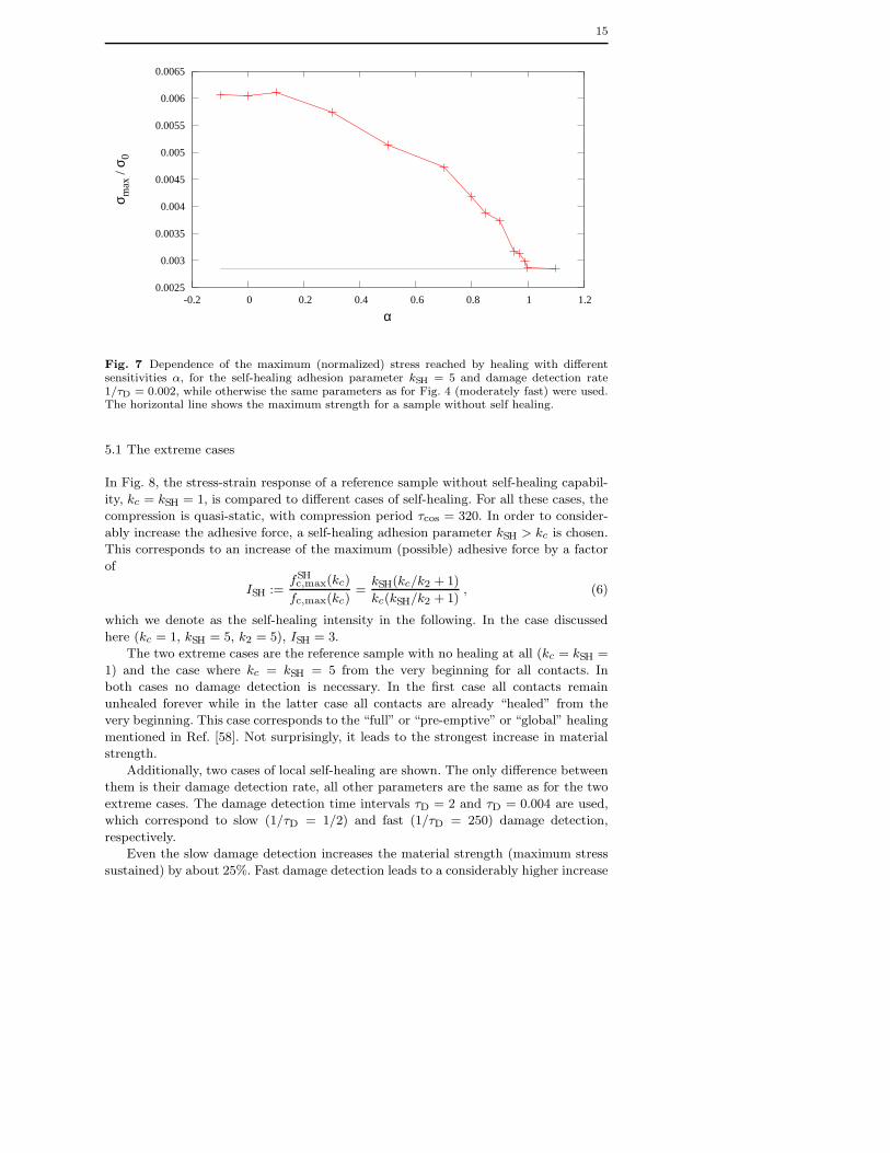
5.1 The extreme cases

In Fig. 8, the stress-strain response of a reference sample without self-healing capabil-

ity, kc = kSH = 1, is compared to different cases of self-healing. For all these cases, the

compression is quasi-static, with compression period τcos = 320. In order to consider-

ably increase the adhesive force, a self-healing adhesion parameter kSH > kc is chosen.

This corresponds to an increase of the maximum (possible) adhesive force by a factor

of

ISH :=fSHc,max(kc)

fc,max(kc)=

kSH(kc/k2 + 1)

kc(kSH/k2 + 1), (6)

which we denote as the self-healing intensity in the following. In the case discussed

here (kc = 1, kSH = 5, k2 = 5), ISH = 3.

The two extreme cases are the reference sample with no healing at all (kc = kSH =

1) and the case where kc = kSH = 5 from the very beginning for all contacts. In

both cases no damage detection is necessary. In the first case all contacts remain

unhealed forever while in the latter case all contacts are already “healed” from the

very beginning. This case corresponds to the “full” or “pre-emptive” or “global” healing

mentioned in Ref. [58]. Not surprisingly, it leads to the strongest increase in material

strength.

Additionally, two cases of local self-healing are shown. The only difference between

them is their damage detection rate, all other parameters are the same as for the two

extreme cases. The damage detection time intervals τD = 2 and τD = 0.004 are used,

which correspond to slow (1/τD = 1/2) and fast (1/τD = 250) damage detection,

respectively.

Even the slow damage detection increases the material strength (maximum stress

sustained) by about 25%. Fast damage detection leads to a considerably higher increase

16

0

0.001

0.002

0.003

0.004

0.005

0.006

0 0.01 0.02 0.03 0.04 0.05 0.06 0.07 0.08

σ / σ

0

ε

kc=11/τD=0.51/τD=250

kc=5

Fig. 8 Stress-strain response of samples with (from top to bottom) “full pre-emptive” healing(kc = 5), fast damage detection rate (1/τD = 250), slow damage detection rate (1/τD = 0.5),and without self-healing (kc = 1).

in strength (about 100% compared to the sample without self-healing), but does not

reach the extreme case of “full” or “pre-emptive” healing, which leads to an increase

of about 150%.

In the following, first, the influence of the damage detection rate is examined in

more detail in subsection 5.2, and second, the effect the healing intensity is studied in

subsection 5.3.

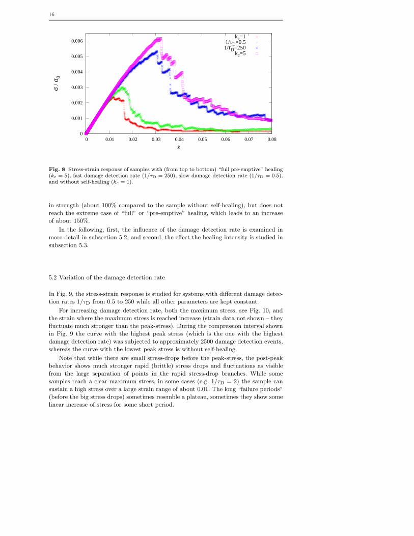
5.2 Variation of the damage detection rate

In Fig. 9, the stress-strain response is studied for systems with different damage detec-

tion rates 1/τD from 0.5 to 250 while all other parameters are kept constant.

For increasing damage detection rate, both the maximum stress, see Fig. 10, and

the strain where the maximum stress is reached increase (strain data not shown – they

fluctuate much stronger than the peak-stress). During the compression interval shown

in Fig. 9 the curve with the highest peak stress (which is the one with the highest

damage detection rate) was subjected to approximately 2500 damage detection events,

whereas the curve with the lowest peak stress is without self-healing.

Note that while there are small stress-drops before the peak-stress, the post-peak

behavior shows much stronger rapid (brittle) stress drops and fluctuations as visible

from the large separation of points in the rapid stress-drop branches. While some

samples reach a clear maximum stress, in some cases (e.g. 1/τD = 2) the sample can

sustain a high stress over a large strain range of about 0.01. The long “failure periods”

(before the big stress drops) sometimes resemble a plateau, sometimes they show some

linear increase of stress for some short period.

17

0

0.001

0.002

0.003

0.004

0.005

0.006

0 0.01 0.02 0.03 0.04 0.05

σ / σ

0

ε

00.5

125

50250

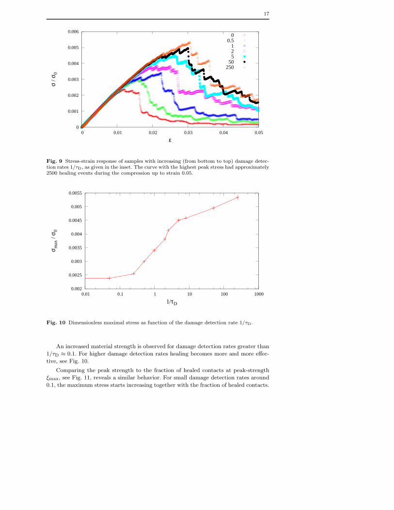
Fig. 9 Stress-strain response of samples with increasing (from bottom to top) damage detec-tion rates 1/τD, as given in the inset. The curve with the highest peak stress had approximately2500 healing events during the compression up to strain 0.05.

0.002

0.0025

0.003

0.0035

0.004

0.0045

0.005

0.0055

0.01 0.1 1 10 100 1000

σ max

/ σ 0

1/τD

Fig. 10 Dimensionless maximal stress as function of the damage detection rate 1/τD.

An increased material strength is observed for damage detection rates greater than

1/τD ≈ 0.1. For higher damage detection rates healing becomes more and more effec-

tive, see Fig. 10.

Comparing the peak strength to the fraction of healed contacts at peak-strength

ξmax, see Fig. 11, reveals a similar behavior. For small damage detection rates around

0.1, the maximum stress starts increasing together with the fraction of healed contacts.

18

0

0.1

0.2

0.3

0.4

0.5

0.6

0.7

0.8

0.01 0.1 1 10 100 1000

ξ max

1/τD

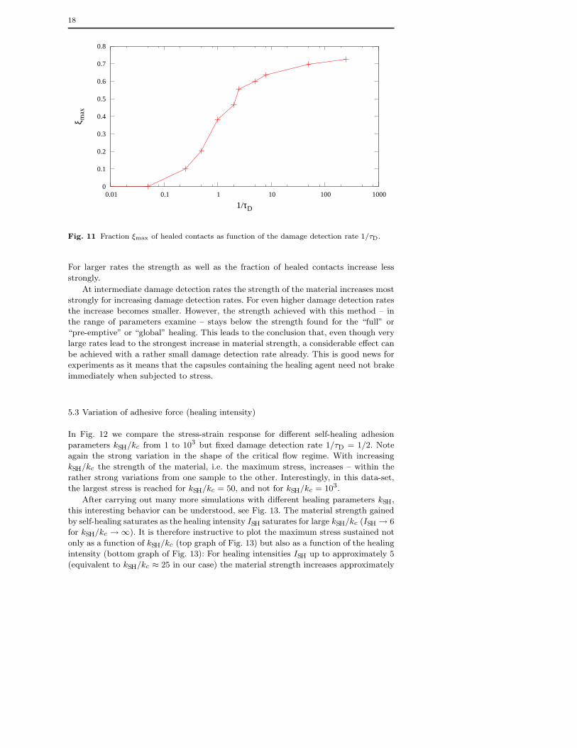
Fig. 11 Fraction ξmax of healed contacts as function of the damage detection rate 1/τD.

For larger rates the strength as well as the fraction of healed contacts increase less

strongly.

At intermediate damage detection rates the strength of the material increases most

strongly for increasing damage detection rates. For even higher damage detection rates

the increase becomes smaller. However, the strength achieved with this method – in

the range of parameters examine – stays below the strength found for the “full” or

“pre-emptive” or “global” healing. This leads to the conclusion that, even though very

large rates lead to the strongest increase in material strength, a considerable effect can

be achieved with a rather small damage detection rate already. This is good news for

experiments as it means that the capsules containing the healing agent need not brake

immediately when subjected to stress.

5.3 Variation of adhesive force (healing intensity)

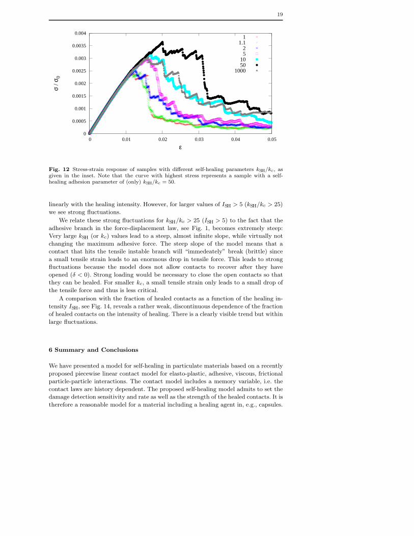
In Fig. 12 we compare the stress-strain response for different self-healing adhesion

parameters kSH/kc from 1 to 103 but fixed damage detection rate 1/τD = 1/2. Note

again the strong variation in the shape of the critical flow regime. With increasing

kSH/kc the strength of the material, i.e. the maximum stress, increases – within the

rather strong variations from one sample to the other. Interestingly, in this data-set,

the largest stress is reached for kSH/kc = 50, and not for kSH/kc = 103.

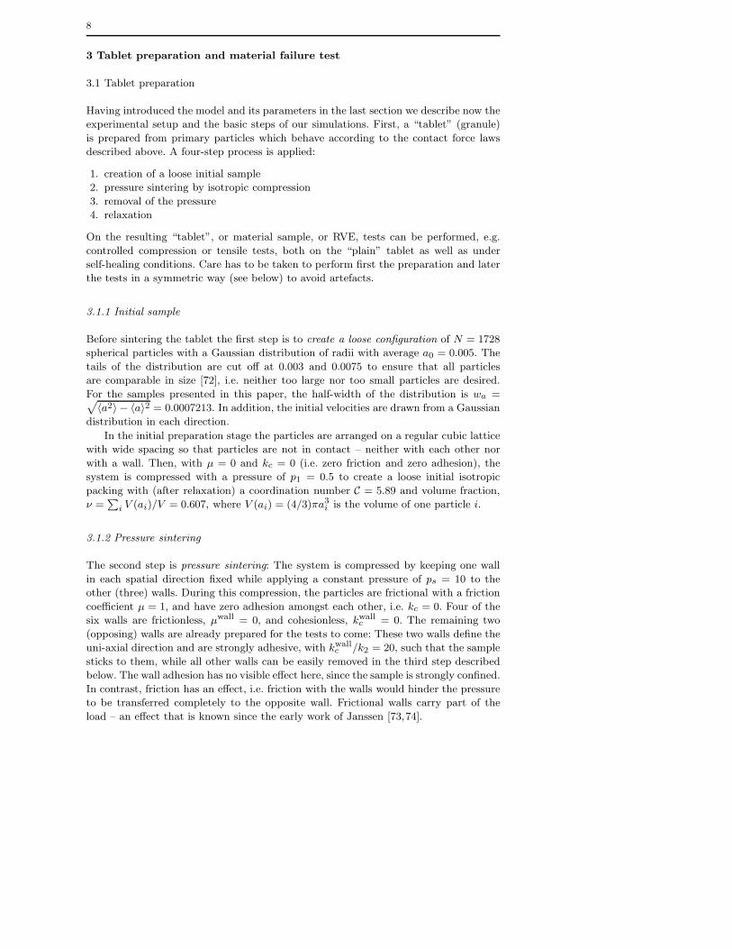
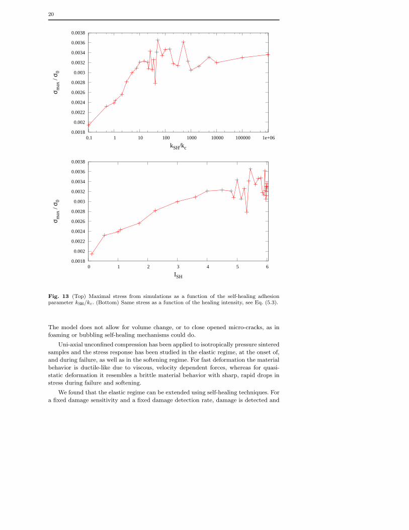
After carrying out many more simulations with different healing parameters kSH,

this interesting behavior can be understood, see Fig. 13. The material strength gained

by self-healing saturates as the healing intensity ISH saturates for large kSH/kc (ISH → 6

for kSH/kc → ∞). It is therefore instructive to plot the maximum stress sustained not

only as a function of kSH/kc (top graph of Fig. 13) but also as a function of the healing

intensity (bottom graph of Fig. 13): For healing intensities ISH up to approximately 5

(equivalent to kSH/kc ≈ 25 in our case) the material strength increases approximately

19

0

0.0005

0.001

0.0015

0.002

0.0025

0.003

0.0035

0.004

0 0.01 0.02 0.03 0.04 0.05

σ / σ

0

ε

11.1

25

1050

1000

Fig. 12 Stress-strain response of samples with different self-healing parameters kSH/kc, asgiven in the inset. Note that the curve with highest stress represents a sample with a self-healing adhesion parameter of (only) kSH/kc = 50.

linearly with the healing intensity. However, for larger values of ISH > 5 (kSH/kc > 25)

we see strong fluctuations.

We relate these strong fluctuations for kSH/kc > 25 (ISH > 5) to the fact that the

adhesive branch in the force-displacement law, see Fig. 1, becomes extremely steep:

Very large kSH (or kc) values lead to a steep, almost infinite slope, while virtually not

changing the maximum adhesive force. The steep slope of the model means that a

contact that hits the tensile instable branch will “immedeately” break (brittle) since

a small tensile strain leads to an enormous drop in tensile force. This leads to strong

fluctuations because the model does not allow contacts to recover after they have

opened (δ < 0). Strong loading would be necessary to close the open contacts so that

they can be healed. For smaller kc, a small tensile strain only leads to a small drop of

the tensile force and thus is less critical.

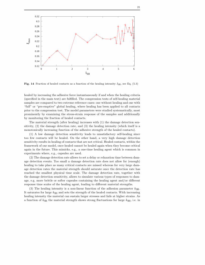
A comparison with the fraction of healed contacts as a function of the healing in-

tensity ISH, see Fig. 14, reveals a rather weak, discontinuous dependence of the fraction

of healed contacts on the intensity of healing. There is a clearly visible trend but within

large fluctuations.

6 Summary and Conclusions

We have presented a model for self-healing in particulate materials based on a recently

proposed piecewise linear contact model for elasto-plastic, adhesive, viscous, frictional

particle-particle interactions. The contact model includes a memory variable, i.e. the

contact laws are history dependent. The proposed self-healing model admits to set the

damage detection sensitivity and rate as well as the strength of the healed contacts. It is

therefore a reasonable model for a material including a healing agent in, e.g., capsules.

20

0.0018

0.002

0.0022

0.0024

0.0026

0.0028

0.003

0.0032

0.0034

0.0036

0.0038

0.1 1 10 100 1000 10000 100000 1e+06

σ max

/ σ 0

kSH/kc

0.0018

0.002

0.0022

0.0024

0.0026

0.0028

0.003

0.0032

0.0034

0.0036

0.0038

0 1 2 3 4 5 6

σ max

/ σ 0

ISH

Fig. 13 (Top) Maximal stress from simulations as a function of the self-healing adhesionparameter kSH/kc. (Bottom) Same stress as a function of the healing intensity, see Eq. (5.3).

The model does not allow for volume change, or to close opened micro-cracks, as in

foaming or bubbling self-healing mechanisms could do.

Uni-axial unconfined compression has been applied to isotropically pressure sintered

samples and the stress response has been studied in the elastic regime, at the onset of,

and during failure, as well as in the softening regime. For fast deformation the material

behavior is ductile-like due to viscous, velocity dependent forces, whereas for quasi-

static deformation it resembles a brittle material behavior with sharp, rapid drops in

stress during failure and softening.

We found that the elastic regime can be extended using self-healing techniques. For

a fixed damage sensitivity and a fixed damage detection rate, damage is detected and

21

0.12

0.14

0.16

0.18

0.2

0.22

0.24

0.26

0.28

0.3

0.32

0 1 2 3 4 5 6

ξ max

ISH

Fig. 14 Fraction of healed contacts as a function of the healing intensity ISH, see Eq. (5.3)

healed by increasing the adhesive force instantaneously if and when the healing criteria

(specified in the main text) are fulfilled. The compression tests of self-healing material

samples are compared to two extreme reference cases: one without healing and one with

“full” or “pre-emptive” global healing, where healing has been applied to all contacts

prior to the compression test. The model parameters were studied systematically, most

prominently by examining the stress-strain response of the samples and additionally

by monitoring the fraction of healed contacts.

The material strength (after healing) increases with (1) the damage detection sen-

sitivity, (2) the damage detection rate, and (3) the healing intensity (which itself is a

monotonically increasing function of the adhesive strength of the healed contacts).

(1) A low damage detection sensitivity leads to unsatisfactory self-healing since

too few contacts will be healed. On the other hand, a very high damage detection

sensitivity results in healing of contacts that are not critical. Healed contacts, within the

framework of our model, once healed cannot be healed again when they become critical

again in the future. This mimicks, e.g., a one-time healing agent which is common in

experiments where, e.g., capsules are used.

(2) The damage detection rate allows to set a delay or relaxation time between dam-

age detection events. Too small a damage detection rate does not allow for (enough)

healing to take place as many critical contacts are missed whereas for very large dam-

age detection rates the material strength should saturate once the detection rate has

reached the smallest physical time scale. The damage detection rate, together with

the damage detection sensitivity, allows to simulate various types of responses to dam-

age, e.g. more brittle or softer capsules containing the healing agent and/or different

response time scales of the healing agent, leading to different material strengths.

(3) The healing intensity is a non-linear function of the adhesion parameter kSH.

It saturates for large kSH and sets the strength of the healed contacts. With increasing

healing intensity the material can sustain larger stresses and fails at higher strains. As

a function of kSH the material strength shows strong fluctuations for large kSH, i.e. in

22

the regime where the healing intensity is almost constant. These fluctuations are due to

local contact instabilities. For very large healing intensities, i.e. for very large adhesive

strength of the healed contacts, a contact rapidly fails when the tensile limit is reached,

resembling a local, brittle failure at the contact level. Thus, moderate values for the

adhesive constant after healing, kSH, lead to the “best” healing results. The fraction of

healed contacts increases a little with the healing intensity, which corresponds to the

final strength of the (solidified) healing agent, i.e. the strength of the final bonding.

To sum up, our model is consistent with, e.g., materials containing healing-agents

in capsules. Once a capsule is broken and local healing has taken place, there cannot

be any further healing at the same position. Different types of capsules and capsule-

matrix interface can be modeled by different damage detection sensitivities and damage

detection rates. Different bonding strengths of the healing agent can be modelled by

adjusting the self-healing adhesive strength kSH.

The quantitative tuning of the DEM model to real experimental data remains a

challenge for future research. The results presented here have units that are not (yet)

supposed to mimick a real material. Some tuning can be done by rescaling, but a real

fine-adjustement will require a comparison with appropriate experimental data.

The model can also be extended to include an additional time scale on which – after

damage is detected and healing is initiated – the strength slowly increases to mimick

the “bonding” or “hardening” of the healing agent. Work along this line is in progress.

Another way to extend this work could be to allow for repeated healing through a

cascade of healing with ever increasing adhesive contact force (at the same position).

The final challenge remains to observe a healing result that is superior to the (much

simpler) global, pre-emptive healing of all contacts.

Acknowledgements

The authors wish to thank Akke Suiker, Orion Mouraille, and Christine Herbst for useful dis-

cussions. This study was supported by the Delft Centre for Materials Self-Healing program,

the research institute IMPACT of the University of Twente, and the Stichting voor Funda-

menteel Onderzoek der Materie (FOM), financially supported by the Nederlandse Organisatie

voor Wetenschappelijk Onderzoek (NWO), through the Granular Matter program.

References

1. R. S. Trask, H. R. Williams, I. P. Bond, Self-healing polymer composites: mimicking natureto enhance performance, Bioinsp. Biomim. 2 (2007) 1–9.

2. C. Dry, Smart bridge and building materials in which cyclic motion is controlled by inter-nally released adhesives, Proceedings of SPIE 2719 (1996) 247–254.

3. G. J. Williams, R. S. Trask, I. P. Bond, A self-healing carbon fibre reinforced polymerfor aerospace applications, Composites Part A: Applied Science and Manufacturing 38 (6)(2007) 1525–1532.

4. M. R. Kessler, Self-healing: a new paradigm in materials design, Proceedings of the IMECH E Part G Journal of Aerospace Engineering 221 (4) (2007) 479–495(17).

5. V. C. Li, Y. M. Lim, Y.-W. Chan, Feasibility study of a passive smart self-healing cemen-titious composite, Composites Part B 29B (1998) 819–827.

6. S. R. White, N. R. Sottos, P. H. Geubelle, J. S. Moore, M. R. Kessler, S. R. Sriram, E. N.Brown, S. Viswanathan, Autonomic healing of polymer composites, Nature 409 (2001)794–797.

23

7. P. Cordier, F. Tournilhac, C. Soulie-Ziakovic, L. Leibler, Self-healing and thermoreversiblerubber from supramolecular assembly, Nature 451 (2008) 977–980.

8. D. A. Abrams, Design of concrete mixtures, Bulletin I, Structural Materials ResearchLaboratory, Lewis Institute, Chicago, Illinois (1918) 309–330.

9. N. Hearn, Self-sealing, autogenous healing and continued hydration: What is the differ-ence?, Materials and Structures/Materiaux et Constructions 31 (1998) 563–567.

10. C. Dry, Matrix cracking repair and filling using active and passive modes for smart timedrelease of chemicals from fibers into cement matrices, Smart Mater. Struct. 3 (1994) 118–123.

11. S. van der Zwaag (Ed.), Self-Healing Materials, Springer, 2007.12. C. Dry, Procedures developed for self-repair of polymeric matrix composite materials,

Composite Structures 35 (1996) 263–269.13. C. M. Dry, Smart-fiber-reinforced matrix composites, U.S. Patent 5,803,963.14. S. R. White, N. R. Sottos, P. H. Geubelle, J. S. Moore, S. R. Sriram, M. R. Kessler, E. N.

Brown, Multifunctional autonomically healing composite material, U.S. Patent 6,518,330.15. E. N. Brown, M. R. Kessler, N. R. Sottos, In-situ poly (urea-formaldehyde) microencap-

sulation of dicyclopentadiene, J. Microencapsulation 20 (2003) 719–730.16. E. N. Brown, J. S. Moore, S. R. White, N. R. Sottos, Fracture and fatigue behavior of a

self-healing polymer, Mat. Res. Soc. Symp. Proc. 735 (2003) C11.22.1.17. E. N. Brown, S. R. White, N. R. Sottos, Retardation and repair of fatigue cracks in a

microcapsule toughened epoxy compositepart ii: in situ self-healing, Compos. Sci. Technol.65 (2005) 2474–2480.

18. R. S. Trask, G. J. Williams, I. P. Bond, Bioinspired self-healing of advanced compositestructures using hollow glass fibres, J. Roy. Soc. Interface 4 (2007) 363–371.

19. F. R. Kersey, D. M. Loveless, S. L. Craig, A hybrid polymer gel with controlled rates ofcross-link rupture and self-repair, J. Roy. Soc. Interface 4 (2007) 373–380.

20. W. Feng, S. H. Patel, M.-Y. Young, J. L. Zunino III, M. Xanthos, Smart polymeric coatings- recent advances, Advances in Polymer Technology 26 (1) (2007) 1–13.

21. D. G. Shchukin, H. Mohwald, Self-repairing coatings containing active nanoreservoirs,SMALL 3 (6) (2007) 926 – 943.

22. R. P. Sijbesma, F. H. Beijer, L. Brunsveld, B. J. B. Folmer, J. H. K. K. Hirschberg, R. F. M.Lange, J. K. L. Lowe, E. W. Meijer, Reversible polymers formed from self-complementarymonomers using quadruple hydrogen bonding, Science 278 (1997) 1601–1604.

23. M. R. Kessler, N. R. Sottos, S. R. White, Self-healing structural composite materials,Composites Part A: Applied Science and Manufacturing 34 (8) (2003) 743–753.

24. T. C. Mauldin, J. D. Rule, N. R. Sottos, S. R. White, J. S. Moore, Self-healing kineticsand the stereoisomers of dicyclopentadiene, J. Roy. Soc. Interface 4 (2007) 389–393.

25. V. J. Soroker, A. J. Denson, Autogenous healing of concrete, Zement 25 (1926) 30.26. F. Brandeis, Autogenous healing of concrete, Beton und Eisen 36 (1937) 12.27. L. Turner, The autogenous healing of cement and concrete - its relation to vibrated concrete

and cracked concrete, Proc. Int Assoc. Testing Materials, Testing Materials, London.28. E. F. Wagner, Autogenous healing of cracks in cement-mortar linings for grey-iron and

ductile-iron watered pipes, J. Am. Water Works Assoc 66 (1974) 358–360.29. S. R. White, S. Maiti, A. S. Jones, E. N. Brown, N. R. Sottos, P. H. Geubelle, Fatigue of

self-healing polymers: multiscale analysis and experiments, preprint (2004).URL http://www.icf11.com/proceeding/EXTENDED/5414.pdf

30. E. Barbero, F. Greco, P. Lonetti, Continuum damage-healing mechanics with applicationto self-healing composites, International Journal of Damage Mechanics 14 (1) (2005) 51–81.

31. H. Peizhen, L. Zhonghua, S. Jun, Finite element analysis on evolution process for damagemicrocrack healing, Acta Mechanica Sinica 16 (3) (2000) 254–263.

32. A. C. Balazs, Modeling self-healing materials, Materials Today 10 (9) (2007) 18–23.33. V. Priman, A. Dementsov, I. Sokolov, Modeling of self-healing polymer composites rein-

forced with nanoporous glass fibers, J. Comp. Theor. Nanosci. 4 (2007) 190–193.34. D. S. Burton, X. Goa, L. C. Brinson, Finite element simulation of a self-healing shape

memory alloy composite, Mechanics of Materials 38 (5-6) (2006) 525–537.35. Y. Guo, W. Guo, Self-healing properties of flaws in nanoscale materials: Effects of soft and

hard molecular dynamics simulations and boundaries studied using a continuum mechan-ical model, Phys. Rev. B 73 (2006) 085411.

36. S. Maiti, C. Shankar, P. H. Geubelle, J. Kieffer, Continuum and molecular-level modelingof fatigue crack retardation in self-healing polymers, Journal of Engineering Materials andTechnology 128 (4) (2006) 595–602.

24

37. H. M. Jaeger, C. Liu, S. R. Nagel, Relaxation at the angle of repose, Phys. Rev. Lett.62 (1) (1989) 40–43.

38. H. M. Jaeger, C. Liu, S. R. Nagel, T. A. Witten, Friction in granular flows, Europhys.Lett.11 (7) (1990) 619–624.

39. H. M. Jaeger, S. R. Nagel, Physics of the granular state, Science 255 (1992) 1523.40. R. P. Behringer, The dynamics of flowing sand, Nonlinear Science Today 3 (1993) 1–15.41. I. Goldhirsch, G. Zanetti, Clustering instability in dissipative gases, Phys. Rev. Lett.

70 (11) (1993) 1619–1622.42. R. P. Behringer, G. W. Baxter, Pattern formation and complexity in granular flow, in:

A. Mehta (Ed.), Granular Matter, 1994, p. 85.43. S. Luding, E. Clement, A. Blumen, J. Rajchenbach, J. Duran, Studies of columns of beads

under external vibrations, Phys. Rev. E 49 (2) (1994) 1634.44. N. Sela, I. Goldhirsch, Hydrodynamic equations for rapid flows of smooth inelastic spheres

to Burnett order, J. Fluid Mech. 361 (1998) 41–74.45. O. Herbst, M. Huthmann, A. Zippelius, Dynamics of inelastically colliding spheres with

Coulomb friction: Relaxation of translational and rotational energy, Granular Matter 2 (4)(2000) 211–219.

46. O. Herbst, R. Cafiero, A. Zippelius, H. J. Herrmann, S. Luding, A driven two-dimensionalgranular gas with Coulomb friction, Phys. Fluids 17 (2005) 107102.

47. A. Santos, Does the Chapman-Enskog expansion for sheared granular gases converge?,Phys. Rev. Lett. 100 (2008) 078003.

48. J. Tomas, Fundamentals of cohesive powder consolidation and flow, Granular Matter6 (2/3) (2004) 75–86.

49. A. Castellanos, The relationship between attractive interparticle forces and bulk behaviorin dry and uncharged fine powders, Advances in Physics 54 (4) (2005) 263–376.

50. S. Luding, Shear flow modeling of cohesive and frictional fine powder, Powder Technology158 (2005) 45–50.

51. S. Luding, Anisotropy in cohesive, frictional granular media, J. Phys.: Condens. Matter17 (2005) S2623–S2640.

52. C. Thornton, K. K. Yin, Impact of elastic spheres with and without adhesion, PowderTechnol. 65 (1991) 153.

53. C. Thornton, K. K. Yin, M. J. Adams, Numerical simulation of the impact fracture andfragmentation of agglomerates, J. Phys. D: Appl. Phys. 29 (1996) 424–435.

54. K. D. Kafui, C. Thornton, Numerical simulations of impact breakage of spherical crys-talline agglomerate, Powder Technology 109 (2000) 113–132.

55. C. Thornton, S. J. Antony, Quasi-static deformation of a soft particle system, PowderTechnology 109 (1-3) (2000) 179–191.

56. S. Luding, K. Manetsberger, J. Muellers, A discrete model for long time sintering, Journalof the Mechanics and Physics of Solids 53(2) (2005) 455–491.

57. S. Luding, Cohesive frictional powders: Contact models for tension, Granular Matter 10(2008) 235–246.

58. S. Luding, A. Suiker, Self-healing of damaged particulate materials through sintering,Philosophical MagazineIn press.

59. P. A. Cundall, O. D. L. Strack, A discrete numerical model for granular assemblies,Geotechnique 29 (1) (1979) 47–65.

60. Y. M. Bashir, J. D. Goddard, A novel simulation method for the quasi-static mechanicsof granular assemblages, J. Rheol. 35 (5) (1991) 849–885.

61. H. J. Herrmann, J.-P. Hovi, S. Luding (Eds.), Physics of dry granular media - NATO ASISeries E 350, Kluwer Academic Publishers, Dordrecht, 1998.

62. C. Thornton, Numerical simulations of deviatoric shear deformation of granular media,Geotechnique 50 (1) (2000) 43–53.

63. C. Thornton, L. Zhang, A DEM comparison of different shear testing devices, in: Y. Kishino(Ed.), Powders & Grains 2001, Balkema, Rotterdam, 2001, pp. 183–190.

64. P. A. Vermeer, S. Diebels, W. Ehlers, H. J. Herrmann, S. Luding, E. Ramm (Eds.), Con-tinuous and Discontinuous Modelling of Cohesive Frictional Materials, Springer, Berlin,2001, lecture Notes in Physics 568.

65. P. A. Vermeer, W. Ehlers, H. J. Herrmann, E. Ramm (Eds.), Modelling of Cohesive-Frictional Materials, Balkema, Leiden, Netherlands, 2004, (ISBN 04 1536 023 4).

66. I. Agnolin, J. T. Jenkins, L. L. Ragione, A continuum theory for a random array ofidentical, elastic, frictional disks., Mechanics of Materials 38(8-10) (2006) 687–701.

25

67. M. Latzel, S. Luding, H. J. Herrmann, D. W. Howell, R. P. Behringer, Comparing simula-tion and experiment of a 2d granular couette shear device, Eur. Phys. J. E 11 (4) (2003)325–333.

68. M. P. Allen, D. J. Tildesley, Computer Simulation of Liquids, Oxford University Press,Oxford, 1987.

69. D. C. Rapaport, The Art of Molecular Dynamics Simulation, Cambridge University Press,Cambridge, 1995.

70. T. Poschel, T. Schwager, Computational Granular Dynamics, Springer, Berlin, 2005.71. S. Luding, E. Clement, A. Blumen, J. Rajchenbach, J. Duran, Anomalous energy dissipa-

tion in molecular dynamics simulations of grains: The “detachment effect”, Phys. Rev. E50 (1994) 4113.

72. C. T. David, R. G. Rojo, H. J. Herrmann, S. Luding, Hysteresis and creep in powders andgrains, in: R. Garcia-Rojo, H. J. Herrmann, S. McNamara (Eds.), Powders and Grains2005, Balkema, Leiden, Netherlands, 2005, pp. 291–294.

73. H. A. Janssen, Versuche uber Getreidedruck in Silozellen, Zeitschr. d. Vereines deutscherIngenieure 39 (35) (1895) 1045–1049.

74. M. Sperl, Experiments on corn pressure in silo cells. translation and comment of janssen’spaper from 1895, Granular Matter 8 (2) (2006) 59–65.

75. J. Schwedes, Review on testers for measuring flow properties of bulk solids, GranularMatter 5 (1) (2003) 1–45.

76. S. Luding, H. J. Herrmann, Micro-macro transition for cohesive granular media, in: BerichtNr. II-7, Inst. fur Mechanik, Universitat Stuttgart, S. Diebels (Ed.) (2001).

77. E. Brown, N. Sottos, Performance of embedded microspheres for self-healing polymercomposites, preprint (2000).URL http://www.autonomic.uiuc.edu/brown files/EricBrownSEM2000.pdf