Modelling of Membrane in a Sodium Sulfate Electrochemical...
80
Modelling of Membrane in a Sodium Sulfate Electrochemical Splitting Cell Master of Science Thesis in the Master’s programme Innovative and Sustainable Chemical Engineering ADNA H. CARLBERG Department of Chemistry and Chemical Engineering Division of Chemical Engineering CHALMERS UNIVERSITY OF TECHNOLOGY Gothenburg, Sweden 2015
Transcript of Modelling of Membrane in a Sodium Sulfate Electrochemical...

Modelling of Membrane in a Sodium
Sulfate Electrochemical Splitting Cell
Master of Science Thesis in the Masterrsquos programme Innovative and Sustainable
Chemical Engineering
ADNA H CARLBERG
Department of Chemistry and Chemical Engineering
Division of Chemical Engineering
CHALMERS UNIVERSITY OF TECHNOLOGY
Gothenburg Sweden 2015
MASTER OF SCIENCE THESIS
Modelling of Membrane in a Sodium
Sulfate Electrochemical Splitting Cell
ADNA H CARLBERG
Supervisors Sara Angervall and Mehdi Arjmand
AkzoNobel Pulp and Performance Chemicals
Examiner Prof Anders Rasmuson
Chalmers Chemical Engineering Design
Department of Chemistry and Chemical Engineering
Division of Chemical Engineering
CHALMERS UNIVERSITY OF TECHNOLOGY
Gothenburg Sweden 2015
Modelling of Membrane in a Sodium Sulfate Electrochemical Splitting Cell
ADNA H CARLBERG
copy ADNA H CARLBERG 2015
Master of Science Thesis
Department of Chemistry and Chemical Engineering
Division of Chemical Engineering
Chalmers University of Technology
SE-412 96 Gothenburg
Sweden
Telephone + 46 (0)31-772 1000
Gothenburg Sweden 2015
v
Modelling of Membrane in a Sodium Sulfate Electrochemical Splitting Cell
ADNA H CARLBERG
Department of Chemistry and Chemical Engineering
Division of Chemical Engineering
Chalmers University of Technology
Abstract
The masterrsquos thesis aims at obtaining a deeper understanding of the transport
phenomena in a sodium sulfate electrochemical splitting cell This is done by modelling
the ion transport through a cation exchange membrane Nafion both with and without
adjacent boundary layers
The resulting model is derived from the Nernst-Planck equation and after some
simplification the model includes the terms diffusion and migration An analytical
solution of the model equation is compared with two numerical solutions by looking at
the concentration profiles for the moving species (sodium ions hydrogen ions and
hydroxyl ions) Also the fluxes of the ions pH water transport and electric potential
through the membrane are investigated by profile plots All profiles show expected
results except the concentration profile in the anolyte film when boundary layers are
added
The main modelling parameters are found to be the bulk concentrations for the
boundary conditions and diffusivities for the ions The potential drop permittivity and
thickness of film layers are found to be important A major limitation of the modelling
procedure in the thesis is though lack of data especially parameters describing the
membranes is difficult to obtain estimates for Apart from the conceptual and
mathematical modelling verification of the mathematical solution by comparison with
formerly obtained results in the literature and finally experimental validation of the
model remain
Keywords electrochemical splitting sodium sulfate Nafion membrane ion transport
Nernst-Planck modelling MATLAB
vii
Acknowledgements
I would like to acknowledge my supervisors Sara Angervall and Mehdi Arjmand for all
their help commitment and advice They have been a great support throughout the
thesis work I would also like to thank the examiner Anders Rasmuson for guidance and
providing valuable input when discussing different ideas
I would like to express my gratitude to Kalle Pelin the department manager of Process
RDampI for giving me the opportunity to conduct the thesis work at AkzoNobel in Bohus
and for giving valuable direction and feedback Also many thanks to all the people at
Process RDampI for a warm welcome to the department and showing interest in the thesis
work
Adna H Carlberg Gothenburg June 2015
ix
Contents
Notations xi
1 Introduction 1
11 Background 1
12 Purpose 2
13 Research questions 2
14 Delimitations 2
15 Thesis outline 3
2 Theory 5
21 Electrochemical splitting 5
211 Nafion membrane structure 6
212 Membrane state 6
22 Chemistry in the cell 7
23 Transport phenomena in the membrane 8
231 Mass transfer of ions 8
232 Mass transfer of solventwater 10
233 Heat transfer 11
234 Momentum transfer 11
24 Boundary layers near membrane surface 12
25 Electrochemical equations 12
3 Methodology 15
31 Literature study 15
32 Modelling procedure 15
33 Solution methods 17
331 Finite difference method 18
332 Boundary and initial conditions 18
34 Experimental setup 18
35 Modelling parameters 19
351 Modelling boundary and initial conditions 21
36 Modelling settings 22
4 Results and Discussion 23
41 Model simplification 23
411 Dimensions and independent variables 23
412 Convection vs diffusion term 24
413 Migration vs diffusion term 24
414 Migration vs convection term 25
415 Final simplified model 26
42 Solution structure of model equations 26
421 Analytical solution of BVP 26
422 Numerical solution of BVP 27
x
423 Numerical solution of PDE 28
43 Concentration and flux profiles 29
44 pH profile 31
45 Electric potential profile 31
46 Water transport 32
47 Boundary layers 33
471 Concentration profiles 33
472 pH profile 34
473 Electric potential profile 35
48 Influence of impurities 36
49 Model limitations 36
491 Model simplifications 37
492 Influence of bi-layer membrane 37
493 Electric potential and electro-neutrality 37
494 Boundary layers close to membrane 38
495 Flow phase of electrolytes 38
496 Experimental validation 39
5 Conclusions 41
6 Future Work 43
References 45
A Modified Nernst-Planck Equation I
B Calculations of Parameters for Modelling III
B1 Calculation of potential drop in boundary layers III
B2 Calculation of permittivity for electrolytes III
B3 Calculation of velocity through the membrane IV
B4 Calculation of free acidity in electrolytes IV
B5 Calculation of sulfonate concentration in membrane V
C Peclet Number VII
D MATLAB-code for Modelling with BVP IX
D1 BVP script file IX
D2 Function files XI
E MATLAB-code for Modelling with PDE XIII
E1 PDE script file XIII
E2 Function files XVI
F Surface Plots for Concentration Profiles XIX
xi
Notations
Variables used in equations in the thesis are presented here with symbol description
and unit
119860 Unit area [m2]
120572 Anolyte volume variation per charge [dm3mol]
120572119894120579 Expression of secondary reference state [dm
3mol]
119862119864 Current efficiency [-]
119888119894 Concentration of species i [moldm3]
119863119894 Diffusion coefficient of species 119894 [m2s]
120575119871 Laminar boundary layer [m]
120575119879 Turbulent boundary layer [m]
119864119882 Equivalent weight [gmol]
휀 Permittivity or dielectric constant [Fm]
휀119903 Relative permittivity [-]
휀0 Vacuum permittivity [Fm]
119865 Faradayrsquos constant [A∙smol]
119891119894 Molar activity coefficient of species 119894 [-]
ℎ Mesh interval [m]
119868 Electric current [A]
119894 Current density [Am2]
119896 Permeability [m2]
119896ℎ Thermal conductivity [JK∙s]
120581 Electronic conductivity [Sm]
119871 Thickness of membrane [m]
119872119894 Molar mass of species 119894 [gmol]
120583 Dynamic viscosity [Pas]
120583119894 Electrochemical potential of species 119894 [Jmol]
119873119894 Flux of species 119894 [molm2∙s]
119899 Number of electrons transferred [-]
119874 Error [mol m2]
119875 Pressure [Pa]
119875119895119894 Perm-selectivity of ion 119894 relative 119895 [-]
119875119890 Peclet number [-]
xii
Φ Electric potential [V]
120601 Porosity [-]
119902 Porous flow [m3m
2∙s]
119902ℎ Heat flow [Jm2∙s]
119877 Ideal gas constant [JmolK]
119877119894 Production rate of species 119894 [moldm3∙s]
119877119890119909 Local Reynolds number [-]
120588 Density [gdm3]
120588119886 Density of anolyte [gdm3]
120588119898 Density of membrane [gdm3]
119904 Active surface area [m2]
119879 Temperature [K]
119879119898119894 Transport number of species 119894 [-]
(based on one ion)
119905 Time [s]
119905119898119894 Transport number of species 119894 [-]
(based on one Faraday)
119906119894 Mobility of species 119894 [m2∙molJ∙s]
119881 Volume [dm3]
119881119886 Volume of anolyte [dm3]
119881119888 Volume of catholyte [dm3]
119881119894 Partial molar volume [m3mol]
119907 Velocity of fluid [ms]
119882 Specific flow rate of water [gm2∙s]
119909 Distance [m]
119911119894 Valencecharge number of species 119894 [-]
1
1 Introduction
The process industry has for the last two centuries found impressive use of earthrsquos
resources It has improved the quality of life for millions of people but sometimes at the
cost of environmental pollutions Taking care of earthrsquos resources in an efficient and
sustainable way both environmentally and economically has been the motivation for
many companies to improve the use of raw material and energy Chemical waste
recovery is one important approach to achieve a sustainable and environmental friendly
process among industries In the pulp and paper industry for instance the Kraft pulp
mills today have often very efficient chemical recovery systems and low losses of
pulping chemicals [1] But with increasing demands on more extensive closure of
systems there exists a continuous need for improving the use of chemicals
11 Background AkzoNobel is an international company that is a supplier of decorative paints
performance coatings and a large number of specialty chemicals One of these specialty
chemicals is sodium chlorate (1198731198861198621198971198743) which is used to produce chlorine
dioxide (1198621198971198742) Chlorine dioxide is a powerful oxidizing agent and it is used as a
bleaching chemical in the pulp industry mostly in the Kraft process [1] Manufacturing
processes of chlorine dioxide [2] result in a by-product which is sodium sulfate
(11987311988621198781198744) and often referred to as salt cake [1 3] It may be beneficial to convert this
by-product into more valuable feedstock such as sodium hydroxide ( 119873119886119874119867 ) and
sulfuric acid (11986721198781198744) see Figure 1 In order to do so one approach is to split the
sodium sulfate using an electrochemical cell including an ion exchange membrane to
promote the selectivity [1 3 4 5 6]
Figure 1 Overview of chemicals involved in the chlorine dioxide production in a single vessel
process (SVP) with salt cake wash (SCW) [2] and in a salt split unit
Sustainability is an important consideration for AkzoNobel in all stages of the value
chain Even if the main objective of the salt split process is to upgrade the value of
the by-product salt there are several interests for developing alternative use of the
sulfate by-product [1 3] In the future there could be limited permissions for emission
of the by-product and disposal can be very costly especially if the sodium sulfate
2
includes impurities [4] For the splitting of sodium sulfate substantial electric energy is
required which may be available on the mill and thus constitute an advantage from a
sustainability perspective as this energy is bio-based [3] The conversion of sodium
sulfate can also give substantial benefits for the pulp mills if cost for raw material
increases [1]
12 Purpose The purpose of the masterrsquos thesis is to obtain a deeper understanding of the
electrochemical processes in a cell for splitting sodium sulfate This will mainly be done
by modelling a cation exchange membrane primarily Nafion 324 to investigate some
of the transport phenomena in the cell It is aimed that the gained knowledge can be
later used for improving the process and the obtained model could be useful for
upscaling to production scale or when using different types of membranes
13 Research questions The focus of this thesis is to investigate what is happening in the cell by studying the
transport phenomena in the membrane For this purpose the following research
questions are considered
What types of model equations are useful to describe the transport of molecules
through the membrane
What parameters are important when deriving a membrane model
How are cations (sodium ions 119873119886+ and hydrogen ions 119867+) transported through
the membrane
How large is the water transport through the membrane based on different
conditions in the cell
How does the proton profile vary from the acidic side to caustic side
How does the ionic concentration profile look like around the membrane
How do other ions (eg calcium ions 1198621198862+ or potassium ions 119870+ ) due to
impurities affect the transportation through the membrane
14 Delimitations The anolyte and catholyte compartments are considered separated and interconnected by
the transport of species through the membrane Initially only the transport across the
membrane is considered but later also boundary layers are included In the thesis
parameters for the Nafion 324 membrane are used as far as possible However the
derived model should be useful for any type of membrane as long as the diffusivities of
the molecules and the thickness of the membrane is known
3
In a large scale salt split cell the composition of the electrolyte void fractions etc at the
inlet and at the outlet of the cell are different Hence the conditions lead to different
results for the transport phenomena However as the dimensions of the electrochemical
cell this work can be validated against are small the modelling only accounts for the
transport in one dimension (perpendicular to the membrane) and the conditions over the
cell passage are averaged to those of a half passage in this thesis
The temperature along the cell passage and between the two compartments in a small
scale salt split cell is very similar Heat transfer over the membrane is thus neglected in
the absence of temperature gradient ie the driving force is zero or very small
In the thesis the modelling of the fluid in the cell is limited to single phase modelling
Thus the two-phase flow nature of the process due to the presence of gas (hydrogen 1198672
and oxygen 1198742) produced at the electrodes is neglected
15 Thesis outline The thesis is composed of 6 chapters a reference list and 6 appendices
Chapter 1 ndash Introduction contains the background and objective for the master thesis is
presented as well as delimitations and research questions for the purpose
The knowledge obtained from the literature study is gathered in Chapter 2 ndash Theory
describing electrochemical splitting with a cation exchange membrane and the
chemistry in the cell The transport phenomena through the membrane are also
described with relevant equations for the modelling of ion transport
Chapter 3 ndash Methodology describes the different steps in the modelling procedure the
experimental setup and the parameter values used in the modelling
The model structure concentration profiles and flux profiles are presented in Chapter 4
ndash Results and Discussion together with the analysis of the results and model limitations
Some the final remarks from the thesis are summarized in Chapter 5 ndash Conclusions
Chapter 6 ndash Future Work includes some recommendations for proceeding modelling
4
5
2 Theory
In this section the theoretical framework for the electrochemical salt split cell is
presented ie electrolysis membrane structure chemistry in the cell and governing
equations for the transport phenomena through the membrane are described
21 Electrochemical splitting
Salt splitting can be achieved by electrolysis In electrolysis chemical compounds are
decomposed by using a direct electric current To perform salt splitting by electrolysis a
cell with two electrodes an anode and a cathode is needed as shown in Figure 2 [7]
The anode is the positive electrode which attracts anions and it is where oxidation
occurs The cathode is the negative electrode which attracts cations and it is where
reduction occurs The cell is filled with electrolyte which is a solution of water or other
solvents in which ions are dissolved [7] The electrolyte blocks the movement of
electrons and by applying a decomposition potential ie the voltage needed for the
electrolysis to occur the motion of the ions towards the charged electrode is made
possible [7 8] The current density can be measured as the electric current per unit cross
section area [8]
Figure 2 A two compartment salt split cell with cation exchange membrane (CEM) [1] (with
permission of copywrite owner)
Cation exchange membrane (CEM) is used to separate the electrolyte into an anolyte
and a catholyte compartment Due to the composition of the membrane it allows the
motion of only cations through the membrane governed by an electrostatic field [1]
Also electro-osmosis which is the motion of solvent (water) through the membrane due
to the applied electrical field can occur [8] which is further described in Section 232
6
211 Nafion membrane structure
The ion exchange membrane used in the electrochemical cell is made up of a polymer
composite matrix called Nafionreg N324 The microstructure of the polymer consists of a
strong hydrophobic fluorocarbonpolytetrafluoroethylene backbone with sidechains
which end with a hydrophilic sulfonic acid [9 10 11] see Figure 3 The Nafion
membrane allows cation transport through the polymer by exchange with the proton
from the sulfonic acid [10] and works as a barrier towards anions by repulsion with the
negatively charged fixed sulfonate groups [8] The hydrated sulfonic acids can also
form inclusions with water which sustain the ion conduction When Nafion is used as a
separator in an electrochemical cell the electron flux on the electrode surface is
balanced by the ion flux through the membrane [10]
Figure 3 The microstructure of the Nafion membrane adapted from [12] (with permission of
copywrite owner)
The N324 is a bi-layer membrane which is reinforced and consists of two sulfonate
layers of different equivalent weight (EW) with different concentration of fixed
negative charge [13] Studies have shown that the membrane consists of a channel
network with very small pore channels in the size range of nanometers [11] The Nafion
membrane 324 is one of the best performing cation exchange membranes based on
current efficiency measurements [13] It has also been shown that the hydraulic
permeability across Nafion membranes increases with increasing temperature and
decreasing equivalent weight [11]
212 Membrane state
There are two models defined for the state of a membrane the acid membrane state and
the alkaline membrane state [4] see Figure 4
7
Figure 4 Model of the acid membrane state (to the left) and the alkaline membrane state
(to the right) of a cation exchange membrane
In the acid membrane state the catholyte concentration has no influence on the current
efficiency because hydroxyl ions have already been neutralized in the acid boundary
layer [4 14] Hydrogen ions pass the membrane when the acid concentration is high and
the sodium hydroxide concentration is low [5]
For the alkaline membrane state the acid concentration in the anolyte has no influence
on the current efficiency because hydrogen ions have already been neutralized in the
alkaline boundary layer [4 14] Hydroxyl ions pass the membrane when the acid
concentration is low and the sodium hydroxide concentration is high [5]
22 Chemistry in the cell The electrochemical splitting of sodium sulfate results in formation of sulfuric acid
(11986721198781198744) and sodium hydroxide (119873119886119874119867) [1] Sodium sulfate is fed to the cell with the
anolyte and water is used for the catholyte see Figure 2
The overall reaction takes place in two steps splitting of water into ions (119867+ and 119874119867minus)
at the electrodes and separation of sodium ions (119873119886+ ) and sulfate ions (1198781198744minus ) by
transportation over the membrane [4] The following reactions occur in the cell [1]
Anode reaction 2 1198672119874 rarr 4 119867+ + 1198742 + 4119890minus (1)
Cathode reaction 4 1198672119874 + 4119890minus rarr 4 119874119867minus + 2 1198672 (2)
Total reaction 6 1198672119874 rarr 4 119874119867minus + 2 1198672 + 4 119867+ + 1198742 (3)
Overall reaction 2 11987311988621198781198744 + 6 1198672119874 rarr 4 119873119886119874119867 + 2 11986721198781198744 + 2 1198672 + 1198742 (4)
Thus in the anode compartment water is oxidized into hydrogen ions and oxygen and in
the cathode compartment water is reduced to hydroxyl ions and hydrogen The overall
reaction is obtained by including sodium sulfate to the total reaction and thus generating
the caustic sodium hydroxide and sulfuric acid as a result
During operation several other reactions might occur due to impurities in the sodium
sulfate as a rest product from the chlorine dioxide production [1] Other phenomena that
8
also may influence the reactions in the cell are for example damages of the membrane
corrosion of the electrodes or electrical issues [15]
23 Transport phenomena in the membrane Sodium ions and hydrogen ions migrate through the cation exchange membrane towards
the cathode due to an induced driving force by the electric field between the electrodes
[1 4 16] The hydrogen ion transfer decreases the current efficiency which varies
either with the ratio of sulfuric acid to total sulfate concentration in the anolyte or with
sodium hydroxide concentration depending on the state of the membrane (acidic or
alkaline) [5] Migration of hydroxide ions is highly undesired [1]
Water transport occurs through the membrane due to electro-osmosis from the anolyte
to catholyte [5] Also it seems that sodium ions migrate through the membrane with four
water molecules per ion and hydrogen ions migrate with three (or less) water molecules
per ion [5] due to coordination chemistry It has been shown that water flux increases in
the current flow direction due to the electro-osmotic drag [16] Due to a pressure
difference in the cell water can also be transported from one cell compartment to the
other [11]
When studying the transport through the cation exchange membrane in the
electrochemical cell one can consider the so-called two-film theory and think of
resistance in series to produce concentration profiles [17] In this thesis the film
resistance is initially neglected due to assumed turbulent bulk flow so the resistance of
the transport of ions lies in the membrane itself Thus only equations describing
transport across the membrane is formulated But even if the flow of electrolyte is
considered turbulent there might be boundary layer effects (film resistance) adjacent to
the surface of the membrane and for this case a boundary layer model is formulated in a
second step
To obtain a model for the ion transport through the membrane some governing
equations are needed The membrane modelling can be done on a molecular
microscopic mesoscopic and macroscopic description level [18] If the transport
process acts as a continuum ie microscopic level the balance equations for
momentum mass and energy are formulated as differential phenomenological equations
and the detailed molecular interactions can be ignored [18]
231 Mass transfer of ions
Nernst-Planck equation describes the molar flux of ions throught the membrane [7 8
13] The equation is only valid for dilute solutions and the transport of the molecules is
a combination of diffusion migration and convection [7 8 19]
119873119894 = minus119863119894nabla119888119894 minus 119911119894119906119894119865119888119894nablaΦ + 119907119888119894 (5)
The diffusion term comes from Fickrsquos law and describes the flow of the species due to a
concentration gradient [19] The migration is due to the gradient of electric potential and
9
the convective part is induced by the bulk motion contribution [17] Since the Nernst-
Planck equation is restricted to dilute solutions it means that solute-solute interactions
are neglected and only solute-solvent interactions are considered [20] To account for
these solute-solute interactions mixture rules with individual diffusion coefficients can
be used [20] Also modifications of the Nernst-Planck equation can be done for
moderately dilute solutions [7] Then a concentration dependent factor for the activity
coefficient in the chemical potential is introduced see Appendix A
The mass conservation law is valid for each ionic species in the solution where the
accumulation of specie 119894 in a control volume is equal to the divergence of the flux
density minusnabla119873119894 and source term 119877119894 [7]
part119888119894
120597119905= minusnabla119873119894 + 119877119894 (6)
Combining the conservation law and Nernst-Planck equation and assuming no reaction
and thus no source term gives the complete Nernst-Planck equation
part119888119894
120597119905= minusnabla(minus119863119894nabla119888119894 minus 119911119894119906119894119865119888119894nablaΦ + 119907119888119894) (7)
Inserting Nernst-Einstein relation equation (8) for the mobility [7] gives
119906119894 =119863119894
119877119879 (8)
part119888119894
120597119905= 119863119894nabla
2119888119894 +119911119894119865119863119894
119877119879nabla119888119894nablaΦ minus 119907nabla119888119894 (9)
For positively charged and negatively charged ions the complete Nernst-Planck
equations are respectively
part119888119894+
120597119905= 119863119894nabla
2119888119894+ +
119911119894119865119863119894
119877119879nabla119888119894
+nablaΦ minus 119907nabla119888119894+ (10)
part119888119894minus
120597119905= 119863119894nabla
2119888119894minus +
119911119894119865119863119894
119877119879nabla119888119894
minusnablaΦ minus 119907nabla119888119894minus (11)
Conservation of volume of the solution is expressed by assuming incompressible
solution [20]
sum Vicii = 1 (12)
The mobility of the cations is determined by their size and electrical properties as well
as the medium structure [8] Assuming no current loss at the inlet and outlet pipes the
current efficiency is equal to the sodium transport number tmNa+ [5] The
dimensionless transport number for sodium is defined as the sodium flux through the
membrane during a certain time divided by the number of moles of charge transferred in
the cell [5]
119905119898119873119886+ =(119881119888[119873119886+]119888)119905+∆119905minus(119881119888[119873119886+]119888)119905
119904∆119905119894119865=
(119881119886[119873119886+]119886)119905+∆119905minus(119881119886[119873119886+]119886)119905
119904∆119905119894119865 (13)
10
The yield can be defined as the membrane perm-selectivity Perm-selective coefficient
of sodium ion relative hydrogen ion 119875119867+119873119886+
[5]
119875119867+119873119886+
=119905119898119873119886+[119867+]
119905119898119867+[119873119886+] (14)
Relations describing the ion transport and thus the current transport in the acidic and
alkaline membrane state [5] are respectively
119905119898119873119886+ + 119905119898119867+ = 1 (15)
119905119898119873119886+ + 119905119898119874119867minus = 1 (16)
232 Mass transfer of solventwater
The solvent ie water in this case can be transported through the ion exchange
membrane in three ways [8] coupling with the electric current passing the membrane
due to the electrical potential gradient (electro-osmosis) transport due to flux of ions
with a hydration shell and transport due to a chemical potential gradient ie
concentration gradient of the solvent (osmotic flux) Depending on the current density
concentration gradient and perm-selectivity of the ion exchange membrane the three
terms can be of different importance [8] If the membrane is high perm-selective and the
difference of salt concentration in the two compartments is moderate the solvent flux
will be dominated by electro-osmosis and flux by hydrated ions [8] This means that the
osmotic solvent flux can be neglected Also due to the hydrophobic perfluorinated
Nafion membrane the water transport occurs mostly by hydrated ions which are
migrating through the membrane as a result of an electrical potential gradient [5 8]
The water flux 1198731198672119874 due to electro-osmosis and thus transportation of hydrated ions
can be approximated by a solvent transport number multiplied by the flux of ions [8]
1198731198672119874 = 1198791198981198672119874 sum 119873119894119894 (17)
The water transport number 1198791198981198672119874 is defined as the number of water molecules
transported through the membrane by one ion The electro-osmotic water transport
number can also be defined as the number of water molecules transported when one
Faraday passes through the system [5 8]
1199051198981198672119874 =1198731198672119874
119894119865=
1198821198721198672119874
119894119865 (18)
The specific flow rate of water through the membrane 119882 can be derived by mass
balance over the anode compartment and assuming constant density of anolyte [5]
119882 =119894
119865(120572120588119886 minus (119905119898119873119886+119872119873119886+ + (1 minus 119905119898119873119886+)119872119867+) minus
1198721198742
4) (19)
If the membrane is in acidic state see Figure 5 the transport number of water represents
the number of water molecules (in this case around three) transported by one mole of
cations (119873119886+ and 119867+) [5] Different cations can have different electro-osmotic transport
11
numbers of water ions with rather large hydration shells can have water transport
number up to eight while for example hydrogen ions have a very low number of less
than three [8]
Figure 5 Water transport number against sulfuric acid to sulfate concentration ratio (a) and
water to sodium molar ratio during transfer through the membrane in the alkaline membrane
state (b) [5] (with permission of Springer Science+Business Media)
An increase of salt concentration can lead to a decrease of water transport number [8]
This is because the perm-selectivity of the membrane decreases with higher salt
concentration and leads to substantial transport of co-ion in the opposite direction
233 Heat transfer
To account for the heat transfer over the membrane an energy balance is derived with
the temperature gradient as driving force The conduction which is described through
Fourier equation can be expressed by [17]
119902ℎ = minus119896ℎ119889119879
119889119909 (20)
In this thesis the temperature gradient between the two compartments in the cell is very
small and a temperature difference of some few degrees will have very limited effect
Also the viscosity and diffusivity coefficient in the membrane is weakly dependent of
the temperature
234 Momentum transfer
Darcyrsquos equation is an expression of conservation of momentum and it is used to
describe the flow through porous material [18]
12
119902 = minus119896
120583
120597119875
120597119909 (21)
The Nafion membrane is seen as a porous polymer material and Darcyrsquos equation is
used to determine the velocity through the membrane which can be calculated by
dividing the flow with the porosity
119907 =119902
120601 (22)
24 Boundary layers near membrane surface Boundary layers (film resistance) at each side of the membrane can be considered to
investigate how the ion concentration profiles look around the membrane Classification
of the boundary layer can be determined by the local Reynolds number [17]
119877119890119909 =120588119907119909
120583 (23)
If 119877119890119909 lt 2 ∙ 105 rarr Laminar boundary layer
If 2 ∙ 105 lt 119877119890119909 lt 3 ∙ 106 rarr Either laminar or turbulent boundary layer
If 119877119890119909 gt 3 ∙ 106 rarr Turbulent boundary layer
For laminar boundary layers the Blasius equation can be used over a flat plate [17]
120575119871 asymp491∙119909
radic119877119890119909 (24)
For a turbulent boundary layer the thickness is [17]
120575119879 asymp0382∙119909
radic119877119890119909 (25)
25 Electrochemical equations Current efficiency (Faradaic efficiency) 119862119864 is the ratio of moles of produced product
from an electrolyte to the maximum theoretical production ie the equivalent number
of moles of electrons passed [13 21]
119862119864 =119899119865119881
119868119905Δ119888119894 (26)
It has been found that the overall current efficiency of the salt split cell is determined by
the performance of the reactions at the electrodes and by the selectivity of the
membrane [1] Also back-migration of hydroxyl ions or undesired reactions in the cell
due to impurities influences the current efficiency negatively To keep high selectivity
and prevent migration of hydrogen ions over the membrane the conversion of sodium
sulfate should be kept at about 50-60 [1] in a two compartment cell
The current through a membrane is assumed to only be carried by ions and the current
density 119894 (index j is also often used) can be expressed by [7 8]
119894 =119868
119860= 119865 sum 119911119894119873119894119894 (27)
13
The current density is also described by Ohmrsquos law [7]
119894 = minus120581nablaΦ (28)
When solving the Nernst-Planck equations the potential distribution is needed The
potential distribution can be described with the Poisson equation where the potential
distribution can be calculated from the ionic concentrations [10 22]
휀nabla2Φ + 119865 sum 119911119894119888119894119894 = 0 (29)
Where the permittivity 휀 is the product of relative permittivity for the medium and the
vacuum permittivity
휀 = 휀119903휀0 (30)
The Poisson equation together with the Nernst-Planck equations forms the Poisson-
Nernst-Planck (PNP) model which is an effective coupling of the transport of individual
ions [22] Poisson equation is used when there is large electric fields and considerable
separation of charges [7] This requires very large electric forces or very small length
scales [22]
It is common to assume electro-neutrality when deriving the potential distribution [7 8
20] This occurs when the net charge either locally or globally is zero meaning that the
negative charge is balanced out by the equally large positive charge [8 10] This
electro-neutrality is expressed by [7]
sum 119911119894119888119894119894 = 0 (31)
Mathematically the electro-neutrality together with the conservation of charge
statement for fairly constant concentrations and constant conductivity can be expressed
by Laplacersquos condition on the potential [7 10]
nabla2Φ = 0 (32)
On a macroscopic scale electro-neutrality is required for any electrolyte solution or for
a solid phase such as the ion-exchange membrane [8] The fixed negative charges in the
Nafion membrane are balanced out by cations meaning that the counter-ions will be
attracted into the membrane and co-ions repelled [8]
14
15
3 Methodology
For the masterrsquos thesis a literature study and a pre-study of the experimental setup was
conducted in order to perform the modelling part and to achieve the aim of the project
Evaluation of the results and report writing are also important parts of the working
process
31 Literature study The literature study was performed throughout the project to increase the knowledge of
the area of interest and to get an understanding of the electrochemical phenomena
present in the salt split cell Also a pre-study of the laboratory setup was done in the
beginning of the project in order to understand the electrochemical cell and to
investigate what data is available for the modelling phase
Searches of literature (reports journal articles books etc) were done in databases
available from AkzoNobel and through Chalmers Library Also searches of internal
publications and reports in AkzoNobel were carried out The main focuses of the
literature study were to find model equations of transport phenomena in membranes to
describe the chemistry in an electrochemical cell and to find data for missing parameters
needed in the modelling part
32 Modelling procedure Modelling of the membrane in the salt split cell is the main focus of the thesis
MATLAB ver8 (R2012b) was used for this purpose The cationic exchange membrane
in a two compartment cell was modeled and some input data from previously conducted
experiments at AkzoNobel was used
Model development consists of different steps and often becomes an iterative procedure
[18] The procedure for the model development used in this thesis is shown in Figure 6
followed by a description of each step [18]
16
Figure 6 The procedure for model development reproduced from [18]
The problem was defined by stating clear goals for the modelling The derived model
should be able to answer the research questions that are stated in the thesis
Formulation of the conceptual model was done in order to identify governing physical
and chemical principles as well as underlying mechanisms Decisions were made on
what hypothesis and assumptions are to include Also data and knowledge about the
relevant topic ie electrolysis with ion transport through a membrane was gathered for
the formulation of the conceptual model
Formulation of the mathematical model was done by representing important quantities
with a suitable mathematical entity for example by a variable Independent and
dependent variables were specified as well as relevant parameters In this case
independent variables are defined as the variable being changed Dependent variables
are the ones being observed due to the change Parameters can either be constants or a
function of other variables
Constraints or limitations for the variables were identified by for example appropriate
magnitude and range Boundary conditions ie what relations that are valid at the
17
systems boundaries and initial conditions for the time-dependent equations were
specified
When the mathematical problem is solved the validity of individual relationships was
checked Analytical solution was compared with numerical solution Also the
mathematical solution was verified by ensuring that the equations are solved correctly
by considering the residuals
Parameters were determined either by constant values or values from the laboratory
setup However some parameters used in the model had to be estimated
If the model has inadequacies it has to be modified by an iterative process see black
arrows in Figure 6 which was done when adding boundary layers near the membrane
into the model For evaluation of the model and how output is affected by uncertainties
in the parameter value of boundary layer thickness sensitivity analysis was performed
After validation and evaluation the model is ready to be applied for the defined purpose
33 Solution methods When modelling the transport of ions together with the equation for the potential the
equations must first be classified in order to choose the appropriate solution method
The derived equations are parabolic second-order non-linear partial differential
equations (PDEs) Therefore the built-in PDE solver in MATLAB pdepe is chosen It
solves initial-boundary value problems for system of PDEs that are parabolic or elliptic
in space variable 119909 and in time 119905 [23] A restriction of the pdepe-solver is that at least
one of the PDEs in the system must be parabolic [23] Since the complete Nernst-Planck
equation is coupled with the equation for the potential these must be solved
simultaneously This is done by defining a system of PDEs
The pdepe-solver converts the PDEs into ordinary differential equations (ODEs) [23]
This is done by a second-order accurate spatial discretization which is based on fixed set
of specified nodes For the time integration the multistep ode15s-solver of variable-
order is used [23] Then both the formula and the time step are changed dynamically
[23] The ode15s-solver is based on numerical differentiation formulas (NDFs) and it
can solve differential-algebraic equations that arise from elliptic equations [24] Ode15s
is also able to solve stiff problems where multiple time scales are present otherwise
causing abrupt fluctuations in the data series [18]
If assuming no accumulation ie no variation of a certain quantity in time the partial
differential equation (PDE) can be simplified to an ordinary differential equation (ODE)
with only one independent variable [18] When solving second-order ODEs in
MATLAB they must first be converted into a system of two first-order ODEs [24] The
ODE can be classified either as an initial-value problem (IVP) or as a boundary-value
problem (BVP) [18]
18
For a boundary value problem the built-in BVP solver in MATLAB bvp4c is used The
bvp4c-solver uses a finite difference code where the three-stage Lobatto IIIa collection
formula is applied and gives a fourth-order accurate solution [25] To solve the BVP an
initial guess of boundary values on the space interval are needed to be specified for the
required solution [25] The mesh selection and error control is determined from the
residuals of the continuous numerical solution at each subinterval
331 Finite difference method
The finite difference method (FDM) or control volume method (CVM) can be used to
solve the governing equations for the transport of ions described by the Nernst-Planck
equation
The central difference for first-order differentials are [7]
d119888119894
d119909|119895=
119888119894(119895+1)minus119888119894(119895minus1)
2ℎ+ 119874(ℎ2) (33)
This introduces an error of order ℎ2 which can be minimized by smaller nodes ie mesh
interval ℎ successively extrapolating to the correct solution Plotting the answer against
ℎ2 should yield a straight line on linear scales [7]
For second-order differentials the central differences are [7]
d2119888119894
d1199092 |119895=
119888119894(119895+1)+119888119894(119895minus1)minus2119888119894(119895)
ℎ2 + 119874(ℎ2) (34)
332 Boundary and initial conditions
When developing mathematical models and solving the derived differential equations
appropriate boundary conditions andor initial conditions are needed The set of
conditions specifies certain values a solution must take at its boundary and for boundary
conditions three types can be used [18]
Dirichlet ndash specifies the value example 119910(0) = 1205741
Neumann ndash specifies the value of the derivative example 120597119910
120597119909|119909=0
= 1205741
Robin ndash specifies a linear combination of the function and its derivative example
1198861119910 + 1198871120597119910
120597119909|119909=0
= 1205741
In this thesis only Dirichlet boundary conditions are specified for the ionic
concentrations and electric potential at the left and right side of the membrane
34 Experimental setup
The experimental setup is described both to get additional understanding for the salt
splitting process and to understand the background for the previously obtained data
19
The lab setup is already built and available for use at AkzoNobel in Bohus The
electrochemical cell is a modified MP-cell (ElectroCell AS Denmark) with a zero gap
configuration on the anode side of the cell The zero gap is due to higher flow rate and
thus higher pressure in the cathode compartment which essentially presses the
membrane onto the anode
The cell includes two electrodes (anode and cathode) one membrane six gaskets and
two spacers see Figure 7 The anode is a DSA (Dimension Stable Anode) made of
titanium with oxygen formation coating and the cathode is made of nickel The
projected area of each electrode is 100 cm2 and the electrodes are surrounded by 1 mm
thick gaskets made of EPDM rubber The Nafion 324 bi-layer membrane is in total
1524 μm thick and the electrode distance is about 2 mm The main layer of the
membrane towards the anolyte is 127 μm with an equivalent weight (EW) of 1100
gmol and on the cathode side there is a barrier layer of 254 μm with equivalent weight
1500 gmol [6] The inflow and outflow of the anolyte respectively catholyte is at the
short side of the spacers which are placed outside of the electrodes The spacers are
meshed to promote the mixing and turbulence of the electrolytes
Figure 7 Structure of the electrochemical cell (not according to dimension)
A rectifier is controlling the current and the voltage is measured over the electrodes
There are instruments to measure the pressure before the cell In a typical case the cell
voltage is 42 V and the pressure difference is 014 bar The voltage drop over the
membrane is 10 of the cell voltage [15] ie 042 V The current density is 35 kAm2
and the operating temperature is set to 80˚C
35 Modelling parameters The constant parameters that are used in the modelling are shown in Table 1
20
Table 1 Constant parameters used in the modelling
Parameter Value
Valence number 119911119873119886+ 1
Valence number 119911119867+ 1
Valence number 119911119874119867minus -1
Faradayrsquos constant 119865 [A∙smol] 96485
Ideal gas constant 119877 [JK∙mol] 83144621
Temperature 119879 [K] 35315
Vacuum permittivity 휀0 [Fm] 885419∙10-12
The parameters that vary in different layers are presented in Table 2 Data for several of
the parameters was not found for the N324-membrane thus literature values for other
similar Nafion membranes (N117 N115) were used The N117-membrane is a
perfluorosulfonic acid CEM with the same equivalent weight as the first layer sulfonate
layer as in N324
Table 2 Variable parameters for different layers and membrane
Parameter Anolyte boundary
layer
Membrane Catholyte
boundary layer
Diffusivity
119863119873119886+ [m2s]
111∙10-9 [26] 098∙10-10 (N117) [5] 111∙10-9 [26]
Diffusivity 119863119867+
[m2s]
333∙10-9 35∙10-10 (N117) [5] 333∙10-9
Diffusivity 119863119874119867minus
[m2s]
443∙10-9 [26] 16∙10-11 (N324) [27] 443∙10-9 [26]
Diffusivity 1198631198672119874
[m2s]
9∙10-10 (N115) [28]
Thickness of
layers 119871 [m]
010∙10-6 50∙10-6 1524∙10-6
(=127∙10-6+253∙10-6)
010∙10-6 50∙10-6
Potential drop
∆Φ [V]
000011550005776
[Appendix B1]
042 000005073000253
6 [Appendix B1]
Relative
permittivity 휀119903
3959
[Appendix B2]
20 (N117) [10 29] 5481
[Appendix B2]
Estimated values for the boundary layers
21
Due to lack of accurate information of the flow properties outside of the membrane
surface for example in terms of the Reynolds number it is difficult to estimate the
boundary layer thickness Three different values from zero to 50 μm are chosen for the
film thickness The potential drop for the different boundary layers is calculated by
using Ohmrsquos law and estimated values for the conductivity see Appendix B1 for
calculations The relative permittivity for the boundary layers is approximated from the
water permittivity see Appendix B2
The membrane is assumed to be homogenously populated with fixed sites and the
modelling is done without considering the ion channels in nanoscale or any molecular
interactions Also the membrane is modelled as one layer but with existence of reliable
parameters and values for ion diffusivity coefficients in the two layers of Nafion 324 the
model would be straight forward to use
Parameters that are used to calculate the velocity of species through the membrane is
presented in Table 3 The dynamic viscosity is in this case an approximation of the
anolyte solution consisting of 21 wt- 11987311988621198781198744 and 14 wt- 11986721198781198744 The direction for
the ion transport is defined positive from the anolyte compartment towards the catholyte
compartment Due to a higher pressure in the catholyte than in the anolyte the velocity
will have a negative value For detailed calculations of the velocity see Appendix B3
Table 3 Parameters used for calculating velocity through the membrane
Parameter Value
Porosity 120601 025 (N117) [30]
Permeability 119896 [m2] 713∙10-20 (N115) [11]
Dynamic viscosity 120583 [Pa∙s] 05∙10-3 (AkzoNobelrsquos database)
Pressure drop ∆119875 [bar] 014 (lab setup)
Velocity 119907 [ms] -52399∙10-13 [Appendix B3]
351 Modelling boundary and initial conditions
The boundary values for the concentrations of the species and electric potential is
shown in Table 4 The concentration of sodium ions is obtained from measurements in
the lab setup as well as for hydroxyl ions in the cathode compartment The hydroxyl
concentration in the anolyte compartment is assumed to be zero since it is very acidic
there (119901119867 = minus011) The boundary concentrations of hydrogen ions are calculated see
Appendix B4 For boundary values for the potential there is no information and
therefore an arbitrary value is chosen at the anolyte side of the membrane in this case
half of the cell voltage and the other boundary is determined by the specified potential
drop over the membrane When adding film layers the calculated potential drops
22
presented in Table 2 for the different layers are added to or subtracted from the
boundary values of the potential
Table 4 Boundary values used in modelling
Parameter Anolyte Catholyte
Sodium 119888119873119886+ [M] 3842 (lab setup) 274 (lab setup)
Hydrogen ion 119888119867+
[M]
15473
[Appendix B4]
37154∙10-12
[Appendix B4]
Hydroxyl 119888119874119867minus [M] 0 274 (lab setup)
Water 1198881198672119874 [M] 455893 537722
Potential Φ [V] 21+
∆Φ119886119899119900119897119910119905119890 119897119886119910119890119903
168-
∆Φ119888119886119905ℎ119900119897119910119905119890 119897119886119910119890119903
Estimated initial conditions for both the membrane and electrolytes in the boundary
layers are shown in Table 5 Before installation in the electrochemical splitting cell the
membrane is placed in 1 wt- 119873119886119874119867
Table 5 Initial conditions used in modelling
Parameter Anolyte Membrane Catholyte
Sodium 119888119873119886+ [M] 4256 02 0
Hydrogen ion 119888119867+
[M]
0 0 0
Hydroxyl 119888119874119867minus [M] 0 02 0
Potential Φ119898 [V] 0 0 0
36 Modelling settings For the numerical solutions some setting values are presented in Table 6
Table 6 Setting values used in modelling
Setting Value in BVP Value in PDE
Mesh nodes 3000 200
Relative residual 10-9 10-3
Absolute residual 10-12 10-6
23
4 Results and Discussion
In this section the modelling of transport phenomena through the membrane is
presented by using the Nernst-Planck equation for the ion transport together with the
Laplace condition for the electrical potential First the model equations are simplified
and then the solution is obtained by simulations in form of profiles followed by
discussion after each part Lastly some model limitations are discussed
41 Model simplification Model simplification is done by reducing the number of dimensions in the geometry and
by reducing the number of independent variables in the modelling equations
The model is further simplified by investigating what terms in the equation that are
significant This is done by comparing the terms describing the ion transport in the
Nernst-Planck equation and determining what mechanisms are the most important for
ion transport through the membrane
411 Dimensions and independent variables
The complete Nernst-Planck equation is a function of time and space and is given in
vectorial form as
part119888119894
120597119905= 119863119894nabla
2119888119894 +119911119894119865119863119894
119877119879nabla119888119894nablaΦ minus 119907nabla119888119894 (9)
Assuming transport in one direction through the membrane only ie the transport of
ions from the anolyte to the catholyte the equation is simplified to (the 119909-direction is
normal to the membrane)
part119888119894(119909119905)
part119905= 119863119894
part2119888119894(119909119905)
part1199092 +119911119894119865119863119894
119877119879
part119888119894(119909119905)
part119909
dΦ(119909119905)
d119909minus 119907
part119888119894(119909119905)
part119909 (35)
The direction in this thesis will always be positive from the anolyte compartment
towards the catholyte compartment
The partial differentials part is approximated with the ordinary differentials d when
solving the equation as a boundary-value problem
d119888119894(119905)
d119905= 119863119894
d2119888119894(119909)
d1199092+
119911119894119865119863119894
119877119879
d119888119894(119909)
d119909
dΦ(119909)
d119909minus 119907
d119888119894(119909)
d119909 (36)
The same simplification is done for the Laplace condition on the potential where the
general equation is given first and then written in one dimension and finally without the
partial differential
nabla2Φ = 0 (32)
1205972Φ(119909119905)
1205971199092 = 0 (37)
d2Φ(119909)
d1199092 = 0 (38)
24
412 Convection vs diffusion term
Comparison between the convection term and the diffusion term from Nernst-Planck
equation is done by creating a ratio in the dimensionless form
119888119900119899119907119890119888119905119894119900119899 = 119907d119888119894
d119909asymp 119907
∆119888
∆119909asymp 119907 (minus
119862
119871)
119889119894119891119891119906119904119894119900119899 = 119863119894
d2119888119894
d1199092asymp 119863119894
∆119888
(∆119909)2asymp 119863119894
119862
1198712
119903119886119905119894119900119862119863 =119888119900119899119907119890119888119905119894119900119899
119889119894119891119891119906119904119894119900119899=
119907(minus119862
119871)
119863119894119862
1198712
= minus119907119871
119863119894= 119889119894119898 119897119890119904119904 (39)
This dimensionless ratio between the convection and diffusion term can be found in the
literature as the Peclet number [17 18]
If 119903119886119905119894119900119862119863 ≪ 1 rarr Total flux asymp diffusional flux
If 119903119886119905119894119900119862119863 asymp 1 rarr Total flux = diffusional flux + convectional flux
If 119903119886119905119894119900119862119863 ≫ 1 rarr Total flux asymp convectional flux
Inserting values for the parameters and the values for the diffusivity coefficients for
each of the ions into equation (39) gives the ratios
119903119886119905119894119900119862119863 = minus119907119871
119863119894=
119863119894 = 119863119873119886+
119863119894 = 119863119867+
119863119894 = 119863119874119867minus
=81486 ∙ 10minus7
22816 ∙ 10minus7
49910 ∙ 10minus6
It can be concluded that the diffusion term completely dominates for all cases and thus
the convection term can be excluded
413 Migration vs diffusion term
A comparison between the migration term and the diffusion term from Nernst-Planck
equation is done by creating a ratio in the dimensionless form
119898119894119892119903119886119905119894119900119899 =119911119894119865119863119894
119877119879
dΦ
d119909
d119888119894
d119909asymp
119911119894119865119863119894
119877119879
dΦ
d119909
∆119888
∆119909asymp
119911119894119865119863119894
119877119879
dΦ
d119909(minus
119862
119871)
119889119894119891119891119906119904119894119900119899 = 119863119894
d2119888119894
d1199092asymp 119863119894
∆119888
(∆119909)2asymp 119863119894
119862
1198712
119903119886119905119894119900119872119863 =119898119894119892119903119886119905119894119900119899
119889119894119891119891119906119904119894119900119899=
119911119894119865119863119894119877119879
dΦ
d119909(minus
119862
119871)
119863119894119862
1198712
= minus119911119894119865
dΦ
d119909119871
119877119879= 119889119894119898 119897119890119904119904 (40)
If 119903119886119905119894119900119872119863 ≪ 1 rarr Total flux asymp diffusional flux
If 119903119886119905119894119900119872119863 asymp 1 rarr Total flux = diffusional flux + migrational flux
If 119903119886119905119894119900119872119863 ≫ 1 rarr Total flux asymp migrational flux
25
The derivative for the potential is assumed to be constant and calculated by using values
at the anolyte side and the catholyte side of the membrane
dΦ
d119909=
Φcat minus Φan
119871asymp
∆Φ
119871
Inserting this together with the other parameters into equation (40) gives the ratio
119903119886119905119894119900119872119863 = minus119911119894119865∆Φ
119877119879= 689988
Since the ratio is larger than 1 the migration term for the Nernst-Planck equation
dominates However since the ratio should be several orders of magnitudes larger to
safely remove a term in order to simplify a model [18] the diffusion term is kept in the
model
Varying the potential at the anolyte side of the membrane from a really low value to
maximal value Φan = (042 42) and assuming the potential drop to 10 gives the
119903119886119905119894119900 = (14 138) This indicates that migration term will be only one ten potential to
maximum two ten potentials larger than the diffusion term Thus it is reasonable to keep
both terms in the model for ion transport
414 Migration vs convection term
Comparing the migration term and the convection term from Nernst-Planck equation is
done by creating a ratio in the dimensionless form
119898119894119892119903119886119905119894119900119899 =119911119894119865119863119894
119877119879
dΦ
d119909
d119888119894
d119909asymp
119911119894119865119863119894
119877119879
dΦ
d119909
∆119888
∆119909asymp
119911119894119865119863119894
119877119879
dΦ
d119909(minus
119862
119871)
119888119900119899119907119890119888119905119894119900119899 = 119907d119888119894
d119909asymp 119907
∆119888
∆119909asymp 119907 (minus
119862
119871)
119903119886119905119894119900119872119862 =119898119894119892119903119886119905119894119900119899
119888119900119899119907119890119888119905119894119900119899=
119911119894119865119863119894119877119879
dΦ
d119909(minus
119862
119871)
119907(minus119862
119871)
=119911119894119865119863119894
dΦ
d119909
119877119879119907= 119889119894119898 119897119890119904119904 (41)
If 119903119886119905119894119900119872119862 ≪ 1 rarr Total flux asymp convectional flux
If 119903119886119905119894119900119872119862 asymp 1 rarr Total flux = convectional + migrational flux
If 119903119886119905119894119900119872119862 ≫ 1 rarr Total flux asymp migrational flux
The derivative for the potential is assumed to be constant and calculated by using values
at the anolyte side and the catholyte side of the membrane
dΦ
d119909=
Φcat minus Φan
119871asymp
∆Φ
119871
Inserting this together with the other parameters and the values for the diffusivity
coefficients for each of the ions into equation (41) gives the ratios
26
119903119886119905119894119900119872119862 =119911119894119865119863119894∆Φ
119877119879119907119871=
119863119894 = 119863119873119886+
119863119894 = 119863119867+
119863119894 = 119863119874119867minus
=84676 ∙ 107
30241 ∙ 108
13825 ∙ 107
The migration term dominates for all cases with several orders of magnitude and thus
the convection term can be excluded This can of course also be concluded directly from
the comparisons above
415 Final simplified model
The Nernst-Planck ion transport model after the afore-mentioned simplifications is
d119888119894
d119905= 119863119894
d2119888119894
d1199092 +119911119894119865119863119894
119877119879
d119888119894
d119909
dΦ
d119909 (42)
For some of the solution approaches steady-state is assumed
42 Solution structure of model equations
The final simplified Nernst-Planck model equation (42) for the ion transport is solved
for the ion concentrations with three approaches analytical solution of BVP numerical
solution of BVP and numerical solution of PDE The resulting solution structure of
these approaches is described in this section followed by some profiles obtained from
the solutions in Sections 43-46
421 Analytical solution of BVP
The analytical solution for Nernst-Planck equation with Laplace condition for the
electrical potential ie constant potential drop across the membrane at steady state is
presented
0 = 119863119894d2119888119894
d1199092 +119911119894119865119863119894
119877119879
∆Φ
∆x
d119888119894
d119909 (43)
0 =d2119888119894
d1199092 +119911119894119865∆Φ
119877119879L
d119888119894
d119909 (44)
Using 119910 = 119888119894(119909) and 119886 =119911119894119865∆Φ
119877119879L a homogeneous equation is obtained
119910primeprime + 119886119910prime = 0 (45)
This is classified as a second-order linear ordinary differential equation and the
auxiliary equation to the homogeneous equation is then
1199032 + 119886119903 = 0 (46)
With the distinct real roots being
1199031 = 0
1199032 = minus119886
Two solutions are obtained from these roots as follows
1199101 = 1198901199031119909 = 1 (47)
27
1199102 = 1198901199032119909 = 119890minus119886119909 (48)
The general solution is then
119910 = 1198601199101 + 1198611199102 = 119860 + 119861119890minus119886119909 (49)
Where 119860 and 119861 are arbitrary constants which can be determined by initial conditions
119910(0) = 1198881 rArr 119860 + 119861 ∙ 1 = 1198881
119910(119871) = 1198882 rArr 119860 + 119861119890minus119886119871 = 1198882
This gives new values for the constants
119860 = 1198881 minus1198882minus1198881
119890minus119886119871minus1 (50)
119861 =1198882minus1198881
119890minus119886119871minus1 (51)
The final analytical solution of the second-order boundary-value problem is
119910 = 1198881 minus1198882minus1198881
119890minus119886119871minus1+
1198882minus1198881
119890minus119886119871minus1119890minus119886119909 (52)
119910 = 1198881 +1198882minus1198881
119890minus119886119871minus1(119890minus119886119909 minus 1) (53)
Written with the original variables the analytical solution is
119888119894(119909) = 1198881 +1198882minus1198881
119890minus
119911119894119865∆Φ
119877119879L119871minus1
(119890minus119911119894119865∆Φ
119877119879L119909 minus 1) (54)
422 Numerical solution of BVP
To solve the Nernst-Planck equation (42) and Laplace equation (38) for the potential as
boundary-value problems in MATLAB functions for the BVP and its boundary
conditions are formulated Firstly steady state d119888119894
d119905= 0 for the Nernst-Planck equation
is assumed which gives
d2119888119894
d1199092 = minus119911119894119865
119877119879
d119888119894
d119909
dΦ
d119909 (55)
This equation must be solved for each species with the additional relation for potential
distribution
d2Φ
d1199092 = 0 (38)
The second-order differential equations are rewritten as a system of two first-order
differential equations to be able to solve them as a boundary-value problem with the
MATLAB bvp4c-solver
1199101 = 119888119894(119909)
y2 =d1199101
d119909(=
d119888119894
d119909)
28
d1199102
d119909=
119911119894119865
119877119879y2
dΦ
d119909(=
d2119888119894
d1199092)
1199103 = Φ(119909)
1199104 =d1199103
d119909(=
dΦ
d119909)
d1199104
d119909= 0(=
d2Φ
d1199092)
Written in the ODE-function in the following form
119889119910119889119909 =
[
1199102
119911119894119865
119877119879y21199104
1199104
0 ]
Dirichlet left and right boundary conditions 119887119888119897 and 119887119888119903 for the functions are specified
at the interval boundaries x0 and xf
119887119888 =
[ 1199101(x0) minus 119887119888119897(119888119894)
1199101(xf) minus 119887119888119903(119888119894)
1199103(x0) minus 119887119888119897(Φ)
1199103(xf) minus 119887119888119903(Φ)]
The MATLAB-code used for the numerical solution is presented in Appendix D
423 Numerical solution of PDE
When solving partial differential equations in the MATLAB pdepe-solver functions for
the PDE initial conditions and the boundary conditions are formulated The Nernst-
Planck PDE (42) and equation for the Laplace PDE (38) potential are solved
simultaneously and rewritten accordingly
1199061 = 119888119894(119909 119905)
1199062 = Φ(119909 119905)
[10] ∙
120597
120597119905[1199061
1199062] =
120597
120597119909∙ [
119863119894
d1199061
d119909+
119911119894119865119863119894
1198771198791199061
d1199062
d119909d1199062
d119909
] + [0 0
]
Initial conditions 119894119888 for both the concentration and potential are specified
1199060 = [119894119888(119888119894)119894119888(Φ)
]
Dirichlet values for the left and right boundary conditions 119887119888119897 and 119887119888119903 are specified in
the following form
29
[1199061 minus 119887119888119897(119888119894)1199062 minus 119887119888119897(Φ)
] + [00] ∙ [
d1199061
d119909d1199062
d119909
] = [00]
[1199061 minus 119887119888119903(119888119894)1199062 minus 119887119888119903(Φ)
] + [00] ∙ [
d1199061
d119909d1199062
d119909
] = [00]
The MATLAB-code used for the numerical solution is presented in Appendix E
43 Concentration and flux profiles
The concentration and flux profiles of sodium ions hydrogen ions and hydroxyl ions
through the membrane are shown in Figure 8 Figure 9 and Figure 10 respectively
The concentration profiles are obtained from the analytical solution of BVP numerical
solution of BVP and numerical solution of PDE For the numerical solution of PDE the
concentration profile for the ions from the last time iteration is used The complete
surface profiles of the PDE solution are shown in Appendix F
The flux profile is obtained from equation (5) with same model simplifications as
described in Section 41 by using the cation concentrations and its derivatives together
with the derivative from the potential from the numerical solution of the BVP
Figure 8 Concentration profile for sodium ions in the membrane from analytical BVP and
PDE solution (in the left plot) and flux profile from BVP solution (in the right plot)
30
Figure 9 Concentration profile for hydrogen ions in the membrane from analytical BVP and
PDE solution (in the left plot) and flux profile from BVP solution (in the right plot)
Figure 10 Concentration profile for hydroxyl ions in the membrane from analytical BVP and
PDE solution (in the left plot) and flux profile from BVP solution (in the right plot)
All concentration profiles from the numerical solutions BVP and PDE resemble the
analytical solution From the concentration profiles for both sodium ions and hydrogen
ions it can be seen that the concentration decrease through the membrane from the
anolyte side to the catholyte side This is expected since there is a concentration
difference across the membrane for the ions with higher concentration at the anolyte
side The profiles show that the decrease starts in the middle of the membrane and is
largest towards the end of the membrane Important to point out is that the solution is
obtained by specifying the boundary values so the solution is affected by these Also it
is important to remember that the sodium ions compete for the fixed sites in the
membrane with hydrogen ions affecting the current efficiency
The profile of hydroxyl ions is mirrored to the cations profiles Even though the
membrane is considered to be in acidic state the transport of hydroxyl ions is simulated
which can be further investigated if relevant All hydroxyl ions should be neutralized at
the right boundary side of the membrane in the case of the acid membrane state as
described in Section 212
31
From all the flux profiles it can be seen that the flux of ions is constant through the
entire membrane which indicates that the flux into the membrane is equal to the flux
out of the membrane This seems reasonable considering the steady-state assumption
Comparing the fluxes it can be seen that the flux of hydrogen ions is a bit higher than
the sodium ion flux This can possibly be explained by that hydrogen ions are smaller
and have a higher diffusivity than sodium ions and thus transport of hydrogen ions
through the membrane is favored Both cations have a positive value of the flux
throughout the membrane while hydroxyl ions have a negative value which is
expected This means that the transport of hydroxyl ions occurs in opposite direction ie
from the catholyte compartment to the anolyte compartment
44 pH profile
The pH profile obtained from the concentration of hydrogen ions from the analytical
solution numerical solution of BVP and numerical solution of PDE is shown in
Figure 11
Figure 11 pH profile in the membrane from analytical BVP and PDE solution
As can be seen from all the concentration profiles for the hydrogen ion most of the
change happens towards the catholyte side of the membrane and thus the same is seen
for the pH profile The solution is once again highly dependent on the boundary values
specified
45 Electric potential profile
The profile for the electric potential from the BVP solution and PDE solution is shown
in Figure 12
32
Figure 12 Electric potential profile in the membrane from BVP solution and PDE solution
As expected from the Laplace expression of the second-order differential equation for
the electric potential the profile is a straight line with constant slope between set
boundary values Even if the values for the potential were not known at the boundaries
the important parameter is the potential drop across the layer of interest in the model
equation for the ion transport For the analytical solution the potential drop is assumed
constant and thus the profile would then look like the potential profiles shown in
Figure 12
46 Water transport
For water transport the transport number due to electro-osmosis and hydrated ions is
used and the profile is seen in Figure 13
The flux profile for water is obtained from equation (17) together with equation (5)
with same model simplifications as described in Section 41 by using the cation
concentrations and its derivatives together with the derivative of the potential from the
numerical solution of the BVP
Figure 13 Concentration profile for water in the membrane from BVP solution (in the left plot)
and flux profile from BVP solution (in the right plot)
33
The water transport through the membrane is considered to be large by looking at the
profiles from the BVP solution compared to the ion concentration and flux profiles in
Section 43 This is expected since the defined water transport is due to electro-osmosis
and transport of hydrated ions The ion-exchange membrane easily lets the cations
through thus water is transported as well
Swelling of membrane due to contact with water changes the thickness of the membrane
and this can also affect the ion transport
47 Boundary layers For profiles through the membrane with boundary layers the same numerical solution
structure with PDEs as described in Section 423 when only modelling the membrane
is used To account for the different layers different diffusion coefficients are specified
see Section 35 Since the profiles through the membrane in Section 43 are very similar
difference on the fourth decimal at the curves of the profiles only the PDE solution is
shown from now on by changing the boundary layer thickness in the MATLAB-code
shown in Appendix E
471 Concentration profiles
The concentration profile from the last time iteration of sodium ions hydrogen ions and
hydroxyl ions through the membrane is shown in Figure 14 Figure 15 and Figure 16
respectively
Figure 14 Concentration profile for sodium ions in the membrane and boundary layers 10 μm
(in the left plot) and 50 μm (in the right plot) from PDE solution
34
Figure 15 Concentration profile for hydrogen ions in the membrane and boundary layers
10 μm (in the left plot) and 50 μm (in the right plot) from PDE solution
Figure 16 Concentration profile for hydroxyl ions in the membrane and boundary layers
10 μm (in the left plot) and 50 μm (in the right plot) from PDE solution
When comparing the resulting plots with different thicknesses it can be seen that the
concentration profile for the ions have the same shape through the membrane even if
boundary layers are added However the magnitude of the profiles varies considerably
ie the wider the boundary layer thickness the higher the concentration of ions inside
the membrane If the film is made thinner than 10 μm the profile will have a lower
increase in the anolyte boundary layer and if the film thickness is made thicker than 50
μm the profile will have a higher increase in the anolyte boundary layer compared to
the concentrations profiles shown above This observation does not have an obvious
explanation Intuitively the concentration profile would decrease towards the
membrane surface and a wider boundary layer thickness would lead to lower
concentration at the surface of the membrane
472 pH profile
The pH profile through the membrane and boundary layers obtained from the
concentration of hydrogen ions is shown in Figure 17
35
Figure 17 pH profile in the membrane and boundary layers 10 μm (in the left plot) and 50 μm
(in the right plot) from PDE solution
When adding boundary layers the alkaline pH values (119901119867 gt 7) are reached in the
second boundary layer in the catholyte compartment rather than inside the membrane
when only the membrane is modelled with bulk values as boundary conditions (see
Figure 11) This result in Figure 17 is favorable since the existence of precipitations
which can occur at high pH due to impurities inside the electrochemical cell can be
avoided
473 Electric potential profile
The profile for the electric potential through the membrane and boundary layers is
shown in Figure 18
Figure 18 Electric potential profile in the membrane and boundary layers 10 μm (in the left
plot) and 50 μm (in the right plot) from PDE solution
The potential drop in the boundary layers is smaller than in the membrane due to higher
conductivity and lower resistance in the solutions Also the relative permittivity is
higher in the solution than in the membrane leading to smaller potential drop It can
however be seen that there is a slightly higher slope for the potential drops in the
boundary layers in Figure 18 compared to the calculated values in Table 2 It cannot be
36
explained why the numerical solver do not interpret the specified condition properly
Attempts have been made with both solvers BVP and PDE however without success It
is though possible to obtain a profile with proper slopes of the electrical potential by
specifying intermediate boundary conditions on the length interval but this approach
then requires boundary conditions for the concentrations as well which is not present
48 Influence of impurities Impurities of other cations in the anolyte and catholyte can influence the desired
transport of the sodium ions In a cation exchange membrane with fixed negative
sulfonate acid groups (1198781198743minus) the counter-ion exchange sequence is [8]
1198611198862+ gt 1198751198872+ gt 1198781199032+ gt 1198621198862+ gt 1198721198922+ gt 119860119892+ gt 119870+ gt 1198731198674+ gt 119873119886+ gt 119871119894+
Considering the counter-ion exchange sequence this indicates that larger monovalent
cations than sodium ions or multivalent ions have larger affinity to the negatively
charged fixed sulfonate groups in the interior of the membrane Intuitively this will
affect the desired sodium transport negatively by decreasing the current efficiency Also
based on the pH the presence of impurities can lead to precipitations inside or on the
surface of the membrane
However how impurities specifically affect the transport through the membrane was
not investigated in the thesis mostly because of lack of data for the diffusivities in the
membrane Also molecular interactions can occur especially for non-dilute solutions
and thus affect the transport of ions Incorporation of this effect into the model is not
straight forward since multicomponent diffusivities are needed which are difficult to
obtain
49 Model limitations
The conceptual modelling and mathematical equations were presented in Chapter 2 the
parameter estimation was presented in Chapter 3 and the solutions of the modelling
equations were presented in this chapter The validity of the model was verified by
using very low residuals fine mesh size for the length dimension and time step intervals
being changed dynamically by the numerical solvers Evaluation of the model
parameters which should be done with independent measurements is not performed in
the thesis Lack of data for several of the parameters is a large factor when assessing the
quality of the model In the present results most membrane specific parameters are
missing for the Nafion 324 membrane Even though appropriate estimates are made it
is important to emphasize that the parameters could be completely different and thus
significantly different results could be expected
The derived model based on the Nernst-Planck equation is limited to dilute solutions
and the activity coefficients are assumed to unity which may not be the case and can
thus influence the result Probably the modified Nernst-Planck equation presented in
Appendix A could be used to cope with this
37
491 Model simplifications
When considering the mass conservation law all transport mechanisms should be
included in a model describing the transport However the simplification of the model
when the convection term is neglected is very reasonable since the membrane is
considered to be very compact and the calculated velocity is very small Of course any
damage of the membrane can lead to pinholes and thus significant convection of species
through the membrane can occur but this is not considered during normal operation
Also for the boundary layers the convection term can safely be neglected when
comparing with the other terms diffusion and migration with several orders of
magnitude to spare This holds even if the diffusivity coefficients in the solvents are one
order of magnitude larger than in the membrane
The geometry and dimensional simplification also is considered appropriate since flow
into the cell is spread out by the meshed spacers and thus the length is probably not
influencing the bulk values considerably This effect however could be significant if the
dimensions of the cell are much larger and the spacers do not have the capability to
spread out the flow evenly
Steady state models are far more usable and relevant than any type of dynamic models
as the typical operation is steady operation and the operational changes resulting in time
dependent parameters can be fully neglected over time For this reason it is sufficient to
use the BVP modelling approach Comparing the plots from the PDE solution with the
BVP solution they are very similar and the graphs almost coincide after some
computational time
492 Influence of bi-layer membrane
In the thesis a mono-layer membrane layer is modelled even if the N324-membrane in
reality is a bi-layer membrane If relevant parameters were known the model can easily
be extended to modelling of the bi-layer membrane Considering the bi-layer membrane
the second layer towards the catholyte side has a higher equivalent weight which means
that the reactivity of the polymer is lower than in the first layer as well as lower
hydraulic permeability There are less active sites in the second layer making it harder
for the ions to go through and thus a protection against the catholyte Based on this the
diffusivities of ions are probably lower in the second layer compared to the diffusivity
coefficients in the first membrane layer The concentration profile through the
membrane would then most likely decrease even further towards the cathode side of the
membrane
493 Electric potential and electro-neutrality
The Laplace expression for the electric potential was derived by the assumption of
electro-neutrality which is considered as an appropriate assumption both for the
solution in the boundary layers and also through the membrane
38
The Laplace condition on the electric potential may however not be appropriate close to
the interface between the membrane and the boundary layers where a charged double
layer with cations can build up This is because the fixed negative charges on the
membrane surface creates an electric field which attracts cations from the solution thus
creating a layer close to the surface of the membrane where the concentration of cations
is higher than in the bulk solution [8] Because of the possibly charged double layer at
the interface between the boundary layers and the membrane the electro-neutrality
assumption would probably not hold here This charged layer is though extremely small
some molecule diameters wide (about 10-10
m) so probably the effect can be neglected
or handled by incorporating some interface relations
Limitation of the Laplace condition on the electric potential is also present close to
electrodes where very strong electric fields are present leading to separation of charges
and thus no electro-neutrality
494 Boundary layers close to membrane
The focus of the modelling has been on the transport of ions through the membrane but
even if the flow regime inside the two compartments in the electrochemical cell is
considered turbulent due to gas evolution at the electrodes and presence of meshed
spacers there is probably a thin laminar boundary layer at the surface of the membrane
It is important to remember that the same model equations were used in all layers and
the only parameters that differed were the diffusivity coefficients permittivity and the
potential drop The same parameter values for the diffusivity coefficients and layer
thickness in the two boundary layers were used which is probably not the case in reality
The ionic diffusivity coefficients are dependent on the concentration of the solution [7]
Due to a higher flow rate of the catholyte the boundary layer on the catholyte side of
the membrane should probably be thinner than the boundary layer thickness on the
anolyte side of the membrane
495 Flow phase of electrolytes
In the current model the multiphase flow nature of the electrolyte is neglected This
assumption is supposed to be acceptable in cells where gas evolution occurs at the
surface of the electrodes typically placed outside of the electrolytes Then the electrolyte
close to the boundary layers should not be affected considerably because of the cell
design However when the electrolyte is placed outside of the electrodes instead as in
the electrochemical cell described in this thesis the gas evolution might have an effect
on the bulk concentrations and thus the results The effect of multiphase flows is
however not incorporated in the modelling and this is not investigated in the thesis It is
believed that single phase modelling is sufficient for this case since the bulk
concentration should not be affected significantly when the electrolyte is considered
well mixed
39
496 Experimental validation
The derived model can only be used in this specific case with the particular
experimental set for the parameters and boundary values Nothing can be said for the
application of the model in other ranges of the parameters To cope with this
independent experiments and comparison to other experimental data is needed
Validation of the model can also be done with reference to literature data for other
similar modelling cases These approaches are however not done in the thesis and
remain for completing the modelling procedure
40
41
5 Conclusions
It can be concluded that the objectives with the thesis are met A model for the transport
through the membrane has been derived and solved Thereby the understanding of the
transport phenomena and parameters relevant for the ion-exchange membrane in a
sodium sulfate electrochemical splitting cell has been significantly clarified
The model equation with the dominating migration and diffusion terms describes the
ion transport through the membrane after some simplifications The main parameters for
the modelling are found to be the bulk concentrations for the boundary conditions and
diffusivities for the ions Also potential drop permittivity and thickness of film layers
are important The rest of the parameters are constants or membrane specifications The
following conclusions can be made from this study
The numerical solutions with the two approaches BVP and PDE give very
similar results as the analytical solution of the model equation when modelling
the transport of sodium ions hydroxyl ions and hydrogen ions through the
membrane The profile for the electric potential is a straight line with constant
slope as expected from the Laplace condition of the potential
Water transport through the membrane is highly affected by the cation
concentration because the main water transport is due to electro-osmosis
together with transport of ions having hydrated shells For this case the transport
number was found to be important for modelling of the water transport
The pH profile show very low acidic values in the anolyte and alkaline values in
the catholyte The location where the transition occurs is found to depend on the
boundary layer thickness Also the ionic concentration profiles depend on the
thickness of the boundary layer and it can be concluded that wider boundary
layer thicknesses give higher concentrations of ions inside the membrane
Impurities with larger or multivalent cations will affect the transport of the
desired sodium ions through the membrane negatively when considering the
counter-ion exchange sequence
For the modelling procedure verification of the mathematical solution by comparing
the solution with formerly obtained results is not performed due to lack of such results
Also experimental validation of the models remains However the derived model and
code is ready for use in MATLAB for further investigation
42
43
6 Future Work
Due to time constraints several aspects of the modelling remain which can be further
improved In the present stage of modelling the transport of ions through the Nafion 324
membrane there are many unknown parameters Hopefully the results from the
estimated parameters until this point can give proper profiles trends and indications but
further work is needed for a more correct and detailed model The following work
would be recommended
Modify the modelling equation to non-dilute case by adding a concentration
dependent factor in the expression for chemical potential
Make new estimates for modelling parameters by experimental measurements
Validate the model by independent experimental results if possible
Ensure good model quality by considering accuracy descriptive realism
precision robustness generality and fruitfulness
Sensitivity analysis for additional parameters with uncertainties
Compare modelling results by using different modelling programs
Consider other description levels of modelling for example molecular scale
Investigate if gas evolution at the electrodes is affecting the results by modelling
the electrolytes as multiphase flows
44
45
References
[1] F Oumlhman L Delin N Simic and K Pelin Electrolysis of sodium sulphate -
efficient use of salt cake and ESP dust in pulp mills AringF Industry amp AkzoNobel
PPC 2014
[2] H Vogt J Balej J E Bennett P Wintzer S Akbar Sheikh P Gallone and K
Pelin Chlorine Oxides and Clorine Oxygen Acids in Ullmanns Encyclopedia of
Industrial Chemistry Weinheim Wiley-VCH Verlag 2010
[3] G Ranger A review of selected electrochemical technologies to manage chlorine
dioxide generator saltcake production and its conversion to useful chemicals
Journal of Science amp Technology for Forest Products and Processes vol 3 no 4
pp 13-18 2013
[4] J Joumlrissen and K H Simmerock The behaviour of ion exchange membranes in
electrolysis and electrodialysis of sodium sulphate Journal of Applied
Electrochemistry vol 21 no 10 pp 869-876 1991
[5] M Rakib P Mocoteacuteguy P Viers E Petit and G Durand Behaviour of Nafion
350 membrane in sodium sulfate electrochemical splitting continuous process
modelling and pilot scale tests Journal of Applied Electrochemistry vol 29 no
12 pp 1439-1448 1999
[6] W Grot Fluorinated Ionomers Oxford Elsevier Inc 2011
[7] J Newman and K E Thomas-Alyea Electrochemical Systems Hoboken John
Wiley amp Sons Inc 2004
[8] H Strathmann Ion-Exchange Membrane Separation Processes Amsterdam
Elsevier BV 2004
[9] Nafion Bulletin 98-04 Nafion N-324 DuPont Product Information
[10] S A Schmidt Mathematical models of ion transport through nafion membranes
in modified electrodes and fuel cells without electroneutrality PhD thesis
University of Iowa 2010
[11] Q Duan H Wang and J Benziger Transport of liquid water through Nafion
membranes Journal of Membrane Science Vols 392-393 pp 88-94 2012
[12] T Tjaumlrnhage Thin Polymer and Phospholipid Films for Biosensors
Characterisation with Gravimetric Electrochemical and Optical Methods PhD
thesis Umearing University 1996
[13] S M Davis G E Gray and P A Kohl Candidate membranes for the
46
electrochemical salt-splitting of Sodium Sulfate Journal of Applied
Electrochemistry vol 38 no 6 pp 777-783 2008
[14] M Paleologou A Thibault P-Y Wong R Thompson and R M Berry
Enhancement of the current efficiency for sodium hydroxide production from
sodium sulphate in a two-compartment bipolar membrane electrodialysis system
Separation and Purification Technology vol 11 pp 159-171 1997
[15] Nafion Bulletin 95-01 Voltage Effects in Membrane Chloralkali Cells DuPont
Technical Information
[16] M J Cheah I G Kevrekidis and J Benziger Effect of interfacial water transport
resistance on coupled proton and water transport across nafion The Journal of
Physical Chemistry B vol 115 pp 10239-10250 2011
[17] J R Welty C E Wicks R E Wilson and G L Rorrer Fundamentals of
Momentum Heat and Mass Transfer Hoboken John Wiley amp Sons 2008
[18] A Rasmuson B Andersson L Olsson and R Andersson Mathematical Modeling
in Chemical Engineering - model formulation simplification and validation
Gothenburg Chalmers University 2013
[19] T A Davis J D Genders and D Pletcher A First Course in Ion Permeable
Membranes Hants The Electrchemical Consultancy 1997
[20] S Psaltis Multicomponent Charge Transport in Electrolyte Solutions PhD
thesis Queensland University of Technology 2012
[21] N Tzanetakis W M Taama and K Scott Salt Splitting in a Three-compartment
membrane Electrolysis Cell Filtration+Separation vol 39 no 3 pp 30-38
2002
[22] K Krabbenhoslashft and J Krabbenhoslashft Application of the Poisson-Nernst-Planck
equations to the migration test Cement and Concrete Research vol 38 pp 77-
88 2008
[23] MathWorks-Documentation Partial Differential Equations The MathWorks Inc
[Online] Available httpukmathworkscomhelpmatlabmathpartial-
differential-equationshtml [Accessed 27 Mars 2015]
[24] MathWorks-Documentation Ordinary Differential Equation The MathWorks
Inc [Online] Available httpukmathworkscomhelpmatlabmathordinary-
differential-equationshtml [Accessed 19 Mars 2015]
[25] MathWorks-Documentation Boundary-Value Problems The MathWorks Inc
[Online] Available httpukmathworkscomhelpmatlabmathboundary-value-
47
problemshtml [Accessed 19 Mars 2015]
[26] P Bosander G Sundstroumlm and E Fontes AkzoNobel internal report 1999
[27] S M Davis Electrochemical splitting of sodium sulfate MSc Thesis Georgia
Institute of Technology 2006
[28] S Motupally A J Becker and J W Weidner Diffusion of Water in Nafion 115
Membranes Journal of The Electrochemical Society vol 147 no 9 pp 3171-
3177 2000
[29] S J Paddison D W Reagor and T A J Zawodzinski High Frequency
Dielectric Studies of Hydrated Nafion Journal of Electroanalytical Chemistry
vol 459 pp 91-97 1998
[30] M W Verbrugge and R F Hill Experimental and Theoretical Investigation of
Perfluorosulfonic Acid Membranes Equilibrated with Aqueous Sulfuric Acid
Solutions The Journal of Physical Chemistry vol 92 no 23 pp 6778-6783
1988
[31] M W Verbrugge E W Schneider R S Conell and R F Hill The effect of
temperature on the equilibrium and transport properties of saturated
poly(perfluorosulfonic acid) membranes Journal of Electrochemical Society vol
139 no 12 pp 3421-3428 1992
[32] E Fontes AkzoNobel internal report 1997
[33] A K Sahu S Pitchumani P Sridhar and A K Shukla Nafion and modified-
Nafion membranes for polymer electrolyte fuel cells An overview Bulletin of
Material Science vol 32 no 3 pp 285-294 2009
48
I
A Modified Nernst-Planck Equation
Using the electrochemical potential as driving force and Nernst-Einstein relation for the
mobility the Nernst-Planck equation becomes [7]
119873119894 = minus119906119894119888119894nabla120583119894 + 119888119894119907 (56)
119873119894 = minus119863119894119888119894
119877119879nabla120583119894 + 119888119894119907 (57)
The gradient of the electric potential nabla120583119894 which depends on the local electrical state
and the local composition can be written as
nabla120583119894 = nabla(120583119894 minus119911119894
119911119899120583119899) +
119911119894
119911119899nabla120583119899 (58)
Where the quasi-electrostatic potential 120583119899 is defined as [7]
120583119899 = 119877119879 ln 119888119899 + 119911119899119865Φ (59)
The expression in the brackets in equation (58) can be written as
120583119894 minus119911119894
119911119899120583119899 = 119877119879 [ln(120572119894
120579119888119894119891119894) minus119911119894
119911119899ln(120572119899
120579119888119899119891119899)] = 119877119879 (ln 120572119894120579 minus
119911119894
119911119899ln 120572119899
120579) +
119877119879 (ln 119888119894 minus119911119894
119911119899ln 119888119899) + 119877119879 (ln 119891119894 minus
119911119894
119911119899ln 119891119899) (60)
At constant temperature equation (58) can be expressed as
nabla120583119894 = 119877119879nabla ln 119888119894 + 119911119899119865nablaΦ + 119877119879nabla(ln 119891119894 minus119911119894
119911119899ln 119891119899) (61)
Inserting equation (61) into (57) the flux expression becomes
119873119894 = minus119911119894119863119894119865
119877119879119888119894nablaΦ minus 119863119894nabla119888119894 minus 119863119894119888119894nabla (ln 119891119894 minus
119911119894
119911119899ln 119891119899) + 119888119894119907 (62)
The ion activity coefficient 119891119894 can then be expressed by
119891119894119899 =119891119894
119891119899119911119894 119911119899frasl (63)
So the final expression for the modified Nernst-Planck equation for moderately diluted
solution is [7]
119873119894 = minus119911119894119863119894119865
119877119879119888119894nablaΦ minus 119863119894nabla119888119894 minus 119863119894119888119894nabla ln 119891119894119899 + 119888119894119907 (64)
II
III
B Calculations of Parameters for Modelling
In this section the calculation for some of the parameters are presented
B1 Calculation of potential drop in boundary layers
The potential drops through the boundary layers can be calculated by the divergence of
potential from Ohmacutes law
119894 = minus120581nablaΦ (28)
rArr nablaΦ = minus119894
120581 (65)
Where the current density and conductivities for different layers are
119894 = 3500 1198601198982
120581119886119899119900119897119910119905119890 = 303 119878119898 (10 wt- 119873119886119874119867 70 ˚C) (AkzoNobelrsquos database)
120581119888119886119905ℎ119900119897119910119905119890 = 69 119878119898 (202 wt- 11987311988621198781198744 and 10 wt- 11986721198781198744 70 ˚C)
(AkzoNobelrsquos database)
Inserting these values into the expression for the divergence of potentialnablaΦ and
multiplying with the specific thickness of each layer 119871 gives the potential difference
∆Φ for the different layers
∆Φ = minus119894
120581119886119899119900119897119910119905119890119871 (66)
∆Φ119886119899119900119897119910119905119890 119897119886119910119890119903 = minus119894
120581119886119899119900119897119910119905119890119871 =
119871 = 10 120583119898119871 = 50 120583119898
=minus0001155 119881minus0005776 119881
∆Φ119888119886119905ℎ119900119897119910119905119890 119897119886119910119890119903 = minus119894
120581119888119886119905ℎ119900119897119910119905119890119871 =
119871 = 10 120583119898119871 = 50 120583119898
=minus00005073 119881minus0002536 119881
The negative value of the potential difference ∆Φ indicates that it is a potential drop
B2 Calculation of permittivity for electrolytes
The permittivity for pure water [30]
휀1199031198672119874 = 78
The water permittivity shows temperature dependence according to following relation
[31]
휀1199031198672119874(119879) = 87836914 minus 0396351 ∙ 119879 + 0000745 ∙ 1198792 (67)
This is valid in the following temperature interval
0 lt 119879 lt 100˚119862 (68)
For the salt split cell 80˚C is used this gives the water permittivity
IV
rArr 휀1199031198672119874 = 119879 = 80˚119862 = 608968
The anolyte contains 65 wt- water and the catholyte contains 90 wt- water which
gives following relative permittivity as an approximation for respective electrolyte
휀119903119886119899119900119897119910119905119890 = 065 ∙ 휀1199031198672119874(119879 = 80˚119862) = 395829
휀119903119888119886119905ℎ119900119897119910119905119890 = 090 ∙ 휀1199031198672119874(119879 = 80˚119862) = 548071
B3 Calculation of velocity through the membrane
The velocity through the membrane is calculated by dividing the flow from Darcyrsquos
equation with the porosity
119907 =119902
120601 (22)
119902 = minus119896
120583
120597119875
120597119909 (21)
rArr 119907 = minus119896
120601120583
∆119875
119871 (69)
Where
119896 = 713 ∙ 10minus20 1198982 (N115) [11]
∆119875 = 014 119887119886119903
119871 = 1524 120583119898 = 1524 ∙ 10minus4 119898
120583 = 5 ∙ 10minus4 119875119886 119904
120601 = 025 (N117) [30]
This gives the velocity through membrane
rArr 119907 = minus52399 ∙ 10minus13 119898119904
B4 Calculation of free acidity in electrolytes
The concentration of hydrogen ions ie the free acidity in the cathode compartment is
calculated by an equation derived for solution of sodium sulfate and sulfuric acid [32]
119888119867+ = 041 ∙ (11988811986721198781198744+ 11988811987311988621198781198744
) (70)
This equation is valid for the following ratio
11988811986721198781198744
11988811986721198781198744+11988811987311988621198781198744
= 05 (71)
Where
11988811986721198781198744= 1853 119872
11988811987311988621198781198744= 1921 119872
This gives the hydrogen ion concentration in the anolyte
V
rArr 119888119867+ = 15473 119872
For the concentration of hydrogen ions in the cathode compartment the measured pH-
value is used
119901119867 = 1143
119888119867+ = log10(119901119867) (72)
rArr 119888119867+ = 37154 ∙ 10minus12 119872
B5 Calculation of sulfonate concentration in membrane
The concentration of the negatively charged sulfonate groups 119888119878 is calculated by the
specified equivalent weight of the two layers of the N324-membrane and assuming they
have the same density as the similar membrane N117 accordingly
119888119878 =120588119898
119864119882 (73)
Where
1198641198821 = 1100 119892119898119900119897 (N324) [6]
1198641198822 = 1500 119892119898119900119897 (N324) [6]
120588119898 = 1740 1198921198891198983 (N117) [10]
rArr 1198881198781 =120588119898
1198641198821=
1740 1198921198891198983
1100 119892119898119900119897= 1582 119872
rArr 1198881198782 =120588119898
1198641198822=
1740 1198921198891198983
1500 119892119898119900119897= 1164 119872
VI
VII
C Peclet Number
The Peclet number is used to estimate what terms for mass transfer in the Nernst-Planck
equation are significant to include in the modelling of the transport of ions through the
membrane
Thickness of the membrane
119871 = 1524 120583119898 = 1524 ∙ 10minus4 119898
Diffusivities for ions through Nafion 117 [5]
119863119873119886+ = 098 ∙ 10minus101198982119904
119863119867+ = 35 ∙ 10minus10 1198982119904
Both the molecular flux and convective flux are significant when 119875119890 asymp 1 Assuming
that 119875119890 = 1 the velocity through the membrane is calculated from the Peclet equation
119875119890 =119907119871
119863119894 (74)
rArr 119907 =119875119890∙119863119894
119871 (75)
119907119873119886+ = minus643 ∙ 10minus7 119898119904
119907119867+ = minus230 ∙ 10minus6 119898119904
These velocities are considered very small and it is important to emphasize that the
pressure gradient is opposite to the concentration gradient ie there is a high
concentration of cations in the anode compartment however the pressure is higher in the
cathode compartment The convective transports due to pressure difference will thus
counteract against the diffusion of cations through the membrane and the velocity will
therefore have a negative value
From the calculated velocity the permeability constant can be calculated by using
Darcyrsquos law This limiting 119896 can be compared with permeability for other membranes to
determine if both diffusion flux and convection should be considered
119902 = minus119896
120583
120597119875
120597119909 (21)
rArr 119896 = minus119902120583∆119909
∆119875 (76)
The pressure difference over the membrane
∆119875 = 014 119887119886119903 (lab setup)
∆119909 = 119871 = 1524 120583119898 = 1524 ∙ 10minus4 119898 (N324)
120583 = 5 ∙ 10minus4 119875119886 119904 (21 wt- 11987311988621198781198744 and 14 wt- 11986721198781198744 80 ˚C) (AkzoNobelrsquos
database)
120601 = 025 (N117) [30]
VIII
119907 =119902
120601 (22)
rArr 119902 = 119907120601 (77)
Flow through membrane for the ions
119902119873119886+ = minus161 ∙ 10minus7 119898119904
119902119867+ = minus574 ∙ 10minus7 119898119904
The permeability for the limiting value of 119875119890 can be calculated
119896 = minus119902120583∆119909
∆119875 (76)
119896119873119886+ = 875 ∙ 10minus14 1198982
119896119867+ = 313 ∙ 10minus13 1198982
Permeability for Nafion N115 from literature [11]
119896 = 713 ∙ 10minus20 1198982
It can be seen that the calculated limiting permeability is much larger order of
magnitude 107 than the permeability found in the literature For the permeability from
literature the Peclet number is
rArr 119875119890 = 88729 ∙ 10minus8
This 119875119890 number is much smaller than 1 indicating that the convective flux can be
neglected in comparison to the diffusional flux
IX
D MATLAB-code for Modelling with BVP
The MATLAB-code used for modelling Nernst-Plank equation as a boundary-value
problem is presented below
D1 BVP script file
MATLAB code for Masterrsquos Thesis in Modelling of Membrane in a Sodium Sulfate Electrochemical Splitting
Cell written by Adna H Carlberg clc clf clear all close all global j MNa MH MO2 S L DNa DH DOH cS z F R T e v cNa_an cNa_cat cH_an
cH_cat cOH_an cOH_cat cH2O_an cH2O_cat U_an U_cat
Input parameters cNa2SO4=1921 Conc of sodium sulfate [M] cNaOH=274 Conc of sodium hydroxide [M] cH2SO4=1853 Conc of sulfuric acid [M] pH_an=-011 pH in anolyte at 80oC pH_cat=1143 pH in catholyte at 80oC rho_an=12653 Density of anolyte [gdm3] rho_cat=10764 Density of anolyte [gdm3] my=05e-3 Dynamic viscosity [Pas](approx from AkzoNobelrsquos
database)
i=3500 Current density [Am2] U_cell=42 Cell voltagepotential [V] U_drop=01U_cell Potential drop 10 over membrane[V](Bulletin 95-
01) U_an=21 GUESS Potential at the anode side of the membrane [V] U_cat=U_an-U_drop Potential at the cathode side of the membrane[V] T=80+27315 Temperature [K] P_an=056 Pressure in the anolyte [bar] P_cat=07 Pressure in the catholyte [bar] z=1 Valencecharge number (Na+ amp H+z=1 OH-z=-1)
Membrane specifications S=100e-4 Active surface area of membrane [m2] L=1524e-6 Thickness of membrane [m] DNa=098e-10 Diffusion coeff for Na+ [m2s](N117)[Rakib-1999] DH=35e-10 Diffusion coeff for H+ [m2s](N117)[Rakib-1999]
DOH=16e-11 Diffusion coeff for OH- [m2s](N324)[Davis-2006] DH2O=9e-10 Diff coeff for H2O [m2s](N115)[Motupallyfig2] e_r=20 Relative permittivity (Nafion 117)[Paddison-
1998Schmidt-2010] cS=15818 Concentration of sulfonate groups [M] k=713e-20 Permeability [m2](Nafion 115)[Duan-2012] phi=025 Porosity [](Nafion 117)[Verbrugge-1988]
Constants F=96485 Faradays number [Asmol] R=83144621 Ideal gas constant [J(Kmol)] e0=885419e-12 Vacuum permittivity [Fm] or [A2s4(kgm3)]
X
MNa2SO4=1420376 Molar mass of sodium sulfate [gmol] MH2SO4=9807354 Molar mass of sulfuric acid [gmol] MNaOH=3999737 Molar mass of sodium hydroxide [gmol] MNa=2299 Molar mass of sodium ion [gmol] MH=100797 Molar mass of hydrogen ion [gmol] MHSO4=9706557 Molar mass of hydrogen sulfate [gmol] MSO4=960576 Molar mass of sulfate ion [gmol] MOH=1700737 Molar mass of hydroxyl ion [gmol] MH2=2100797 Molar mass of hydrogen [gmol] MO2=2159994 Molar mass of oxygen [gmol] MH2O=1801534 Molar mass of water [gmol]
Calculated values cNa_an=2cNa2SO4 Conc of Na+ in the anolyte [M] cNa_cat=cNaOH Conc of Na+ in the catholyte [M] cOH_an=0 GUESS Conc of OH- in the catholyte [M] cOH_cat=cNaOH Conc of OH- in the catholyte [M]
conversion=cH2SO4(cH2SO4+cNa2SO4) Use eq6 from [Fontes-1997] cH_an=041(cH2SO4+cNa2SO4) Conc of H+ in the anolyte [M][Fontes-1997] cH_an=10^-pH_an Conc of H+ in the anolyte calc from pH cH_cat=10^-pH_cat Conc of H+ in the catholyte calc from pH
cH2O_an=(06491rho_an)MH2O cH2O_cat=(09rho_cat)MH2O
e=e_re0 Absolute permittivity of Nafion [FM] q=-(k(P_cat-P_an))(myL) Flow through membrane [m3(m2s)] v=qphi Velocity through the membrane [ms]
Solving BVP with Laplace disp(BVP-Laplace) solinit=bvpinit(linspace(0L100)[cNa_an 0 cH_an 0 cOH_an 0 cH2O_an
0 U_an 0]) solinit=bvpinit(linspace(0L3000)[cNa_an ((cNa_cat-cNa_an)L) cH_an
((cH_cat-cH_an)L) cOH_an ((cOH_cat-cOH_an)L) U_an cH2O_an
((cH2O_cat-cH2O_an)L) ((U_cat-U_an)L)]) same solution when guessing slope for the profile ie derivative options=bvpset(StatsonRelTol 1e-9AbsTol[1e-12 1e-12 1e-12
1e-12 1e-12 1e-12 1e-12 1e-12 1e-12 1e-12]) sol=bvp4c(odefunLodebcsolinitoptions) xint=linspace(0L) Sxint=deval(solxint)
figure(1) plot(xintSxint(1)g) plots conc Na+ vs x xlabel(Distance [m]) ylabel(Concentration Na^+ [M]) figure(2) plot(xintSxint(3)r) plots conc H+ vs x xlabel(Distance [m]) ylabel(Concentration H^+ [M]) figure(3) plot(xintSxint(5)k) plots conc OH- vs x xlabel(Distance [m]) ylabel(Concentration OH^- [M])
XI
figure(4) plot(xintSxint(7)b) plots potential vs x xlabel(Distance [m]) ylabel(Electric potential [V]) figure(5) plot(xint-log10(Sxint(3))r) plots pH vs x xlabel(Distance [m]) ylabel(pH profile) figure(6) plot(xintSxint(9)b) plots conc H2O vs x xlabel(Distance [m]) ylabel(Concentration H_2O [M])
Calculating and plotting fluxes Ni_Na=-DNaSxint(2)-((zFDNaSxint(1)Sxint(8))(RT)) Ni_H=-(DHSxint(4))-((zFDHSxint(3)Sxint(8))(RT)) Ni_OH=-DOHSxint(6)-((-zFDOHSxint(5)Sxint(8))(RT)) Ni_H2O=4Ni_Na+3Ni_H
figure(7) plot(xintNi_Nag) xlabel(Distance [m]) ylabel(Flux of Na^+ [molm^2s]) figure(8) plot(xintNi_Hr) xlabel(Distance [m]) ylabel(Flux of H^+ [molm^2s]) figure(9) plot(xintNi_OHk) xlabel(Distance [m]) ylabel(Flux of OH^- [molm^2s]) figure(10) plot(xintNi_H2Ob) xlabel(Distance [m]) ylabel(Flux of H_2O [molm^2s])
D2 Function files
function [dydx]=odefunL(xy) System of 10 first-order ODEs global z F R T dydx(1)=y(2) conc Na+ dydx(2)=-((zF)(RT))y(8)y(2) dydx(3)=y(4) conc H+ dydx(4)=-((zF)(RT))y(8)y(4) dydx(5)=y(6) conc OH- dydx(6)=-((-zF)(RT))y(8)y(6) dydx(7)=y(8) Potential dydx(8)=0 Laplace dydx(9)=y(10) conc H2O dydx(10)=(-4(dydx(2)+((zF)(RT))y(8)y(2))-
3(dydx(4)+((zF)(RT))y(8)y(4))) dydx=dydx end
XII
function [res]=odebc(yayb) Boundary conditions for 10 first-order ODEs global cNa_an cNa_cat cH_an cH_cat cOH_an cOH_cat cH2O_an cH2O_cat
U_an U_cat res(1)=ya(1)-cNa_an res(2)=yb(1)-cNa_cat res(3)=ya(3)-cH_an res(4)=yb(3)-cH_cat res(5)=ya(5)-cOH_an res(6)=yb(5)-cOH_cat res(7)=ya(7)-U_an res(8)=yb(7)-U_cat res(9)=ya(9)-cH2O_an res(10)=yb(9)-cH2O_cat res=res end
XIII
E MATLAB-code for Modelling with PDE
The MATLAB-code used for modelling Nernst-Plank as partial differential equations is
presented below
E1 PDE script file
MATLAB code for Masterrsquos Thesis in Modelling of Membrane in a Sodium Sulfate Electrochemical Splitting
Cell written by Adna H Carlberg clc clf clear all close all global F L L2 DNa1 DH1 DOH1 DNa2 DH2 DOH2 DH2O z R T e1 e_a e_c cNa_an
cNa_cat cH_an cH_cat cOH_an cOH_cat L1 DNa_a DH_a DOH_a L3 DNa_c DH_c
DOH_c U_an U_cat U_a U_c
Input parameters cNa2SO4=1921 Conc of sodium sulfate [M] cNaOH=274 Conc of sodium hydroxide [M] cH2SO4=1853 Conc of sulfuric acid [M] pH_an=-011 pH in anolyte at 80oC pH_cat=1143 pH in catholyte at 80oC rho_an=12653 Density of anolyte [gdm3] rho_cat=10764 Density of anolyte [gdm3] my=05e-3 Dynamic viscosity [Pas](approx from AkzoNobelrsquos
database)
i=3500 Current density [Am2] U_cell=42 Cell voltagepotential [V] U_drop=01U_cell Potential drop 10 over membrane [V] (Bulletin
95-01) U_an=21 GUESS Potential at the anode side of the
membrane [V] U_cat=U_an-U_drop Potential at the cathode side of the membrane [V] T=80+27315 Temperature [K] e_w=87836914-0396351T+0000745TT Permittivity for water
[Verbrugge-1992] P_an=056 Pressure in the anolyte [bar] P_cat=07 Pressure in the catholyte [bar] z=1 Valencecharge number (Na+ amp H+z=1 OH-z=-1)
Membrane specifications S=100e-4 Active surface area of membrane [m2] L=1524e-6 Thickness of membrane in total [m] L2=127e-6 Thickness of membrane layer towards the anolyte [m] DNa1=098e-10 Diffusion coeff for sodium ion [m2s](Nafion
117)[Rakib-1999] DH1=35e-10 Diffusion coeff for hydrogen ion [m2s](Nafion
117)[Rakib-1999] DOH1=16e-11 Diffusion coeff for hydroxyl ion [m2s](Nafion
324)[Davis-2006] DH2O1=9e-10 Diffusion coeff for water [m2s](Nafion
115)[Motupally fig 2]
XIV
e_r=20 Relative permittivity (Nafion 117)[Paddison-
1998Schmidt-2010] cS=15818 Conc of sulfonate groups [M] k=713e-20 Permeability [m2](Nafion 115)[Duan-2012] phi=025 Porosity [](Nafion 117)[Verbrugge-1988]
Boundary layer on anolyte side L1=10e-6 GUESS Film thickness [m] K_an=303 Conductivity of the anolyte [Sm]
(AkzoNobelrsquos database) U_drop_an=(iK_an)L1 Potential drop over the anolyte boundary
layer [V] U_a=U_an+U_drop_an Potential at the anolyte side of the film [V] DNa_a=111e-9 Diffusivity of sodium ion [m2s][Bosander-1999] DH_a=333e-9 GUESS 3 times higher than DNa_a [m2s] DOH_a=443e-9 Diffusivity of hydroxyl ion [m2s][Bosander-
1999]
Boundary layer on catholyte side L3=10e-6 GUESS Film thickness [m] K_cat=69 Conductivity of the anolyte [Sm]
(AkzoNobelrsquos database) U_drop_cat=(iK_cat)L3 Potential drop over the catholyte boundary
layer [V] U_c=U_cat-U_drop_cat Potential at the catholyte side of the film
[V] DNa_c=111e-9 Diffusivity of sodium ion [m2s][Bosander-1999] DH_c=333e-9 GUESS 3 times higher than DNa_c [m2s] DOH_c=443e-9 Diffusivity of hydroxyl ion [m2s][Bosander-
1999]
Constants F=96485 Faradays number [Asmol] R=83144621 Ideal gas constant [J(Kmol)] e0=885419e-12 Vacuum permittivity [Fm] or [A2s4(kgm3)]
MNa2SO4=1420376 Molar mass of sodium sulfate [gmol] MH2SO4=9807354 Molar mass of sulfuric acid [gmol] MNaOH=3999737 Molar mass of sodium hydroxide [gmol] MNa=2299 Molar mass of sodium ion [gmol] MH=100797 Molar mass of hydrogen ion [gmol] MHSO4=9706557 Molar mass of hydrogen sulfate [gmol] MSO4=960576 Molar mass of sulfate ion [gmol] MOH=1700737 Molar mass of hydroxyl ion [gmol] MH2=2100797 Molar mass of hydrogen [gmol] MO2=2159994 Molar mass of oxygen [gmol] MH2O=1801534 Molar mass of water [gmol]
Calculated values cNa_an=2cNa2SO4 Conc of Na+ in the anolyte [M] cNa_cat=cNaOH Conc of Na+ in the catholyte [M] cOH_an=0 GUESS Conc of OH- in the catholyte [M] cOH_cat=cNaOH Conc of OH- in the catholyte [M]
conversion=cH2SO4(cH2SO4+cNa2SO4) Use eq6 from [Fontes-1997] cH_an=041(cH2SO4+cNa2SO4) Conc of H+ in the anolyte [M][Fontes-1997] cH_an=10^-pH_an Conc of H+ in the anolyte calc from pH cH_cat=10^-pH_cat Conc of H+ in the catholyte calc from pH
XV
cH2O_an=(06491rho_an)MH2O cH2O_cat=(09rho_cat)MH2O
e1=e_re0 Absolute permittivity of Nafion [FM] e_a=e_w065e0 Absolute permittivity of boundary layer
on anolyte side [FM] e_c=e_w09e0 Absolute permittivity of boundary layer
on catholyte side [FM] q=-(k(P_cat-P_an))(myL) Flow through membrane [m3(m2s)] v=qphi Velocity through the membrane [ms]
Numerical solution (Membrane+2 boundary layers) tic xmesh=linspace(0(L1+L+L3)200) tspan=linspace(010001e4) m=0 sol=pdepe(mpdefunL2pdeic2pdebc2xmeshtspan) u1=sol(1) Na+ u2=sol(2) H+ u3=sol(3) OH- u4=sol(4) potential toc
Plots figure(1) create new figure surf(xmeshtspanu1) 3D-plot with axis xyz xlabel(Distance [m]) ylabel(Time [s]) zlabel(Conc [M]) figure(2) plot(xmeshu1(end)g) plots the conc profile at the last time xlabel(Distance [m]) ylabel(Concentration Na^+ [M]) line([L1 L1][26 4]) line([L1+L L1+L][26 4])
figure(3) surf(xmeshtspanu2) 3D-plot with axis xyz xlabel(Distance [m]) ylabel(Time [s]) zlabel(Conc [M]) figure(4) plot(xmeshu2(end)r) plots the conc profile at the last time xlabel(Distance [m]) ylabel(Concentration H^+ [M]) line([L1 L1][0 18]) line([L1+L L1+L][0 18])
figure(5) plot(xmesh-log10(u2(end))r) plots y vs x xlabel(Distance [m]) ylabel(pH profile) line([L1 L1][-2 12]) line([L1+L L1+L][-2 12])
XVI
figure(6) surf(xmeshtspanu3) 3D-plot with axis xyz xlabel(Distance [m]) ylabel(Time [s]) zlabel(Conc [M]) figure(7) plot(xmeshu3(end)k) plots the conc profile at the last time xlabel(Distance [m]) ylabel(Concentration OH^- [M]) line([L1 L1][0 3]) line([L1+L L1+L][0 3])
figure(8) surf(xmeshtspanu4) 3D-plot with axis xyz xlabel(Distance [m]) ylabel(Time [s]) zlabel(Conc [M]) figure(9) plot(xmeshu4(end)) plots the potential profile at the last time xlabel(Distance [m]) ylabel(Electric potential [V]) line([L1 L1][16 21]) line([L1+L L1+L][16 21])
E2 Function files
function [afs]=pdefunL2(xtududx) Coefficients for rewritten PDEs global F L L2 DNa1 DH1 DOH1 DNa2 DH2 DOH2 z R T e1 e_a e_c L1 DNa_a
DH_a DOH_a DNa_c DH_c DOH_c
If one membrane layer if xlt=L1 DNa=DNa_a DH=DH_a DOH=DOH_a e=e_a elseif xgt(L1+L) DNa=DNa_c DH=DH_c DOH=DOH_c e=e_c else DNa=DNa1 DH=DH1 DOH=DOH1 e=e1 end
If two membrane layers if xlt=L1 DNa=DNa_a DH=DH_a DOH=DOH_a elseif xgtL1 ampamp xlt=(L1+L2) DNa=DNa1 DH=DH1
XVII
DOH=DOH1 elseif xgt(L1+L) DNa=DNa_c DH=DH_c DOH=DOH_c else DNa=DNa2 DH=DH2 DOH=DOH2 end
a=[1110] one column [NaHOHpotential] f=[((dudx(1)DNa)+((zFDNau(1)dudx(4))(RT))) ((dudx(2)DH)+((zFDHu(2)dudx(4))(RT))) ((dudx(3)DOH)+((-zFDOHu(3)dudx(4))(RT))) -edudx(4)] s=[0000] end
function [u0]=pdeic2(x) Initial condition for PDEs global L1 L
if xlt=L1 u0=[4256000] elseif xgt(L1+L) u0=[020020] elseif xgtL1 ampamp xlt=(L1+L) u0=[0000] end end
function [plqlprqr]=pdebc2(xlulxrurt) Boundary conditions for PDEs global cNa_an cNa_cat cH_an cH_cat cOH_an cOH_cat U_an U_cat U_a U_c
pl=[ul(1)-cNa_an ul(2)-cH_an ul(3)-cOH_an ul(4)-U_a] ql=[0000] derivative pr=[ur(1)-cNa_cat ur(2)-cH_cat ur(3)-cOH_cat ur(4)-U_c] qr=[0000] end
XVIII
XIX
F Surface Plots for Concentration Profiles
The surface plots for the concentration profiles for the ions in time and space from the
PDE solution is presented in this section The end time for the time interval in the
pdepe-solver is chosen so that the profiles are no longer changing shape Important to
point out is that the intervals are made coarser here in these plots to be able to
distinguish the colors and change of shape of the concentration profile the beginning of
time interval
Figure 19 Concentration profile in time and space for sodium ions from PDE solution
XX
Figure 20 Concentration profile in time and space for hydrogen ions from PDE solution
Figure 21 Concentration profile in time and space for hydroxyl ions from PDE solution

Modelling of Membrane in a Sodium Sulfate Electrochemical Splitting Cell
ADNA H CARLBERG
copy ADNA H CARLBERG 2015
Master of Science Thesis
Department of Chemistry and Chemical Engineering
Division of Chemical Engineering
Chalmers University of Technology
SE-412 96 Gothenburg
Sweden
Telephone + 46 (0)31-772 1000
Gothenburg Sweden 2015
v
Modelling of Membrane in a Sodium Sulfate Electrochemical Splitting Cell
ADNA H CARLBERG
Department of Chemistry and Chemical Engineering
Division of Chemical Engineering
Chalmers University of Technology
Abstract
The masterrsquos thesis aims at obtaining a deeper understanding of the transport
phenomena in a sodium sulfate electrochemical splitting cell This is done by modelling
the ion transport through a cation exchange membrane Nafion both with and without
adjacent boundary layers
The resulting model is derived from the Nernst-Planck equation and after some
simplification the model includes the terms diffusion and migration An analytical
solution of the model equation is compared with two numerical solutions by looking at
the concentration profiles for the moving species (sodium ions hydrogen ions and
hydroxyl ions) Also the fluxes of the ions pH water transport and electric potential
through the membrane are investigated by profile plots All profiles show expected
results except the concentration profile in the anolyte film when boundary layers are
added
The main modelling parameters are found to be the bulk concentrations for the
boundary conditions and diffusivities for the ions The potential drop permittivity and
thickness of film layers are found to be important A major limitation of the modelling
procedure in the thesis is though lack of data especially parameters describing the
membranes is difficult to obtain estimates for Apart from the conceptual and
mathematical modelling verification of the mathematical solution by comparison with
formerly obtained results in the literature and finally experimental validation of the
model remain
Keywords electrochemical splitting sodium sulfate Nafion membrane ion transport
Nernst-Planck modelling MATLAB
vii
Acknowledgements
I would like to acknowledge my supervisors Sara Angervall and Mehdi Arjmand for all
their help commitment and advice They have been a great support throughout the
thesis work I would also like to thank the examiner Anders Rasmuson for guidance and
providing valuable input when discussing different ideas
I would like to express my gratitude to Kalle Pelin the department manager of Process
RDampI for giving me the opportunity to conduct the thesis work at AkzoNobel in Bohus
and for giving valuable direction and feedback Also many thanks to all the people at
Process RDampI for a warm welcome to the department and showing interest in the thesis
work
Adna H Carlberg Gothenburg June 2015
ix
Contents
Notations xi
1 Introduction 1
11 Background 1
12 Purpose 2
13 Research questions 2
14 Delimitations 2
15 Thesis outline 3
2 Theory 5
21 Electrochemical splitting 5
211 Nafion membrane structure 6
212 Membrane state 6
22 Chemistry in the cell 7
23 Transport phenomena in the membrane 8
231 Mass transfer of ions 8
232 Mass transfer of solventwater 10
233 Heat transfer 11
234 Momentum transfer 11
24 Boundary layers near membrane surface 12
25 Electrochemical equations 12
3 Methodology 15
31 Literature study 15
32 Modelling procedure 15
33 Solution methods 17
331 Finite difference method 18
332 Boundary and initial conditions 18
34 Experimental setup 18
35 Modelling parameters 19
351 Modelling boundary and initial conditions 21
36 Modelling settings 22
4 Results and Discussion 23
41 Model simplification 23
411 Dimensions and independent variables 23
412 Convection vs diffusion term 24
413 Migration vs diffusion term 24
414 Migration vs convection term 25
415 Final simplified model 26
42 Solution structure of model equations 26
421 Analytical solution of BVP 26
422 Numerical solution of BVP 27
x
423 Numerical solution of PDE 28
43 Concentration and flux profiles 29
44 pH profile 31
45 Electric potential profile 31
46 Water transport 32
47 Boundary layers 33
471 Concentration profiles 33
472 pH profile 34
473 Electric potential profile 35
48 Influence of impurities 36
49 Model limitations 36
491 Model simplifications 37
492 Influence of bi-layer membrane 37
493 Electric potential and electro-neutrality 37
494 Boundary layers close to membrane 38
495 Flow phase of electrolytes 38
496 Experimental validation 39
5 Conclusions 41
6 Future Work 43
References 45
A Modified Nernst-Planck Equation I
B Calculations of Parameters for Modelling III
B1 Calculation of potential drop in boundary layers III
B2 Calculation of permittivity for electrolytes III
B3 Calculation of velocity through the membrane IV
B4 Calculation of free acidity in electrolytes IV
B5 Calculation of sulfonate concentration in membrane V
C Peclet Number VII
D MATLAB-code for Modelling with BVP IX
D1 BVP script file IX
D2 Function files XI
E MATLAB-code for Modelling with PDE XIII
E1 PDE script file XIII
E2 Function files XVI
F Surface Plots for Concentration Profiles XIX
xi
Notations
Variables used in equations in the thesis are presented here with symbol description
and unit
119860 Unit area [m2]
120572 Anolyte volume variation per charge [dm3mol]
120572119894120579 Expression of secondary reference state [dm
3mol]
119862119864 Current efficiency [-]
119888119894 Concentration of species i [moldm3]
119863119894 Diffusion coefficient of species 119894 [m2s]
120575119871 Laminar boundary layer [m]
120575119879 Turbulent boundary layer [m]
119864119882 Equivalent weight [gmol]
휀 Permittivity or dielectric constant [Fm]
휀119903 Relative permittivity [-]
휀0 Vacuum permittivity [Fm]
119865 Faradayrsquos constant [A∙smol]
119891119894 Molar activity coefficient of species 119894 [-]
ℎ Mesh interval [m]
119868 Electric current [A]
119894 Current density [Am2]
119896 Permeability [m2]
119896ℎ Thermal conductivity [JK∙s]
120581 Electronic conductivity [Sm]
119871 Thickness of membrane [m]
119872119894 Molar mass of species 119894 [gmol]
120583 Dynamic viscosity [Pas]
120583119894 Electrochemical potential of species 119894 [Jmol]
119873119894 Flux of species 119894 [molm2∙s]
119899 Number of electrons transferred [-]
119874 Error [mol m2]
119875 Pressure [Pa]
119875119895119894 Perm-selectivity of ion 119894 relative 119895 [-]
119875119890 Peclet number [-]
xii
Φ Electric potential [V]
120601 Porosity [-]
119902 Porous flow [m3m
2∙s]
119902ℎ Heat flow [Jm2∙s]
119877 Ideal gas constant [JmolK]
119877119894 Production rate of species 119894 [moldm3∙s]
119877119890119909 Local Reynolds number [-]
120588 Density [gdm3]
120588119886 Density of anolyte [gdm3]
120588119898 Density of membrane [gdm3]
119904 Active surface area [m2]
119879 Temperature [K]
119879119898119894 Transport number of species 119894 [-]
(based on one ion)
119905 Time [s]
119905119898119894 Transport number of species 119894 [-]
(based on one Faraday)
119906119894 Mobility of species 119894 [m2∙molJ∙s]
119881 Volume [dm3]
119881119886 Volume of anolyte [dm3]
119881119888 Volume of catholyte [dm3]
119881119894 Partial molar volume [m3mol]
119907 Velocity of fluid [ms]
119882 Specific flow rate of water [gm2∙s]
119909 Distance [m]
119911119894 Valencecharge number of species 119894 [-]
1
1 Introduction
The process industry has for the last two centuries found impressive use of earthrsquos
resources It has improved the quality of life for millions of people but sometimes at the
cost of environmental pollutions Taking care of earthrsquos resources in an efficient and
sustainable way both environmentally and economically has been the motivation for
many companies to improve the use of raw material and energy Chemical waste
recovery is one important approach to achieve a sustainable and environmental friendly
process among industries In the pulp and paper industry for instance the Kraft pulp
mills today have often very efficient chemical recovery systems and low losses of
pulping chemicals [1] But with increasing demands on more extensive closure of
systems there exists a continuous need for improving the use of chemicals
11 Background AkzoNobel is an international company that is a supplier of decorative paints
performance coatings and a large number of specialty chemicals One of these specialty
chemicals is sodium chlorate (1198731198861198621198971198743) which is used to produce chlorine
dioxide (1198621198971198742) Chlorine dioxide is a powerful oxidizing agent and it is used as a
bleaching chemical in the pulp industry mostly in the Kraft process [1] Manufacturing
processes of chlorine dioxide [2] result in a by-product which is sodium sulfate
(11987311988621198781198744) and often referred to as salt cake [1 3] It may be beneficial to convert this
by-product into more valuable feedstock such as sodium hydroxide ( 119873119886119874119867 ) and
sulfuric acid (11986721198781198744) see Figure 1 In order to do so one approach is to split the
sodium sulfate using an electrochemical cell including an ion exchange membrane to
promote the selectivity [1 3 4 5 6]
Figure 1 Overview of chemicals involved in the chlorine dioxide production in a single vessel
process (SVP) with salt cake wash (SCW) [2] and in a salt split unit
Sustainability is an important consideration for AkzoNobel in all stages of the value
chain Even if the main objective of the salt split process is to upgrade the value of
the by-product salt there are several interests for developing alternative use of the
sulfate by-product [1 3] In the future there could be limited permissions for emission
of the by-product and disposal can be very costly especially if the sodium sulfate
2
includes impurities [4] For the splitting of sodium sulfate substantial electric energy is
required which may be available on the mill and thus constitute an advantage from a
sustainability perspective as this energy is bio-based [3] The conversion of sodium
sulfate can also give substantial benefits for the pulp mills if cost for raw material
increases [1]
12 Purpose The purpose of the masterrsquos thesis is to obtain a deeper understanding of the
electrochemical processes in a cell for splitting sodium sulfate This will mainly be done
by modelling a cation exchange membrane primarily Nafion 324 to investigate some
of the transport phenomena in the cell It is aimed that the gained knowledge can be
later used for improving the process and the obtained model could be useful for
upscaling to production scale or when using different types of membranes
13 Research questions The focus of this thesis is to investigate what is happening in the cell by studying the
transport phenomena in the membrane For this purpose the following research
questions are considered
What types of model equations are useful to describe the transport of molecules
through the membrane
What parameters are important when deriving a membrane model
How are cations (sodium ions 119873119886+ and hydrogen ions 119867+) transported through
the membrane
How large is the water transport through the membrane based on different
conditions in the cell
How does the proton profile vary from the acidic side to caustic side
How does the ionic concentration profile look like around the membrane
How do other ions (eg calcium ions 1198621198862+ or potassium ions 119870+ ) due to
impurities affect the transportation through the membrane
14 Delimitations The anolyte and catholyte compartments are considered separated and interconnected by
the transport of species through the membrane Initially only the transport across the
membrane is considered but later also boundary layers are included In the thesis
parameters for the Nafion 324 membrane are used as far as possible However the
derived model should be useful for any type of membrane as long as the diffusivities of
the molecules and the thickness of the membrane is known
3
In a large scale salt split cell the composition of the electrolyte void fractions etc at the
inlet and at the outlet of the cell are different Hence the conditions lead to different
results for the transport phenomena However as the dimensions of the electrochemical
cell this work can be validated against are small the modelling only accounts for the
transport in one dimension (perpendicular to the membrane) and the conditions over the
cell passage are averaged to those of a half passage in this thesis
The temperature along the cell passage and between the two compartments in a small
scale salt split cell is very similar Heat transfer over the membrane is thus neglected in
the absence of temperature gradient ie the driving force is zero or very small
In the thesis the modelling of the fluid in the cell is limited to single phase modelling
Thus the two-phase flow nature of the process due to the presence of gas (hydrogen 1198672
and oxygen 1198742) produced at the electrodes is neglected
15 Thesis outline The thesis is composed of 6 chapters a reference list and 6 appendices
Chapter 1 ndash Introduction contains the background and objective for the master thesis is
presented as well as delimitations and research questions for the purpose
The knowledge obtained from the literature study is gathered in Chapter 2 ndash Theory
describing electrochemical splitting with a cation exchange membrane and the
chemistry in the cell The transport phenomena through the membrane are also
described with relevant equations for the modelling of ion transport
Chapter 3 ndash Methodology describes the different steps in the modelling procedure the
experimental setup and the parameter values used in the modelling
The model structure concentration profiles and flux profiles are presented in Chapter 4
ndash Results and Discussion together with the analysis of the results and model limitations
Some the final remarks from the thesis are summarized in Chapter 5 ndash Conclusions
Chapter 6 ndash Future Work includes some recommendations for proceeding modelling
4
5
2 Theory
In this section the theoretical framework for the electrochemical salt split cell is
presented ie electrolysis membrane structure chemistry in the cell and governing
equations for the transport phenomena through the membrane are described
21 Electrochemical splitting
Salt splitting can be achieved by electrolysis In electrolysis chemical compounds are
decomposed by using a direct electric current To perform salt splitting by electrolysis a
cell with two electrodes an anode and a cathode is needed as shown in Figure 2 [7]
The anode is the positive electrode which attracts anions and it is where oxidation
occurs The cathode is the negative electrode which attracts cations and it is where
reduction occurs The cell is filled with electrolyte which is a solution of water or other
solvents in which ions are dissolved [7] The electrolyte blocks the movement of
electrons and by applying a decomposition potential ie the voltage needed for the
electrolysis to occur the motion of the ions towards the charged electrode is made
possible [7 8] The current density can be measured as the electric current per unit cross
section area [8]
Figure 2 A two compartment salt split cell with cation exchange membrane (CEM) [1] (with
permission of copywrite owner)
Cation exchange membrane (CEM) is used to separate the electrolyte into an anolyte
and a catholyte compartment Due to the composition of the membrane it allows the
motion of only cations through the membrane governed by an electrostatic field [1]
Also electro-osmosis which is the motion of solvent (water) through the membrane due
to the applied electrical field can occur [8] which is further described in Section 232
6
211 Nafion membrane structure
The ion exchange membrane used in the electrochemical cell is made up of a polymer
composite matrix called Nafionreg N324 The microstructure of the polymer consists of a
strong hydrophobic fluorocarbonpolytetrafluoroethylene backbone with sidechains
which end with a hydrophilic sulfonic acid [9 10 11] see Figure 3 The Nafion
membrane allows cation transport through the polymer by exchange with the proton
from the sulfonic acid [10] and works as a barrier towards anions by repulsion with the
negatively charged fixed sulfonate groups [8] The hydrated sulfonic acids can also
form inclusions with water which sustain the ion conduction When Nafion is used as a
separator in an electrochemical cell the electron flux on the electrode surface is
balanced by the ion flux through the membrane [10]
Figure 3 The microstructure of the Nafion membrane adapted from [12] (with permission of
copywrite owner)
The N324 is a bi-layer membrane which is reinforced and consists of two sulfonate
layers of different equivalent weight (EW) with different concentration of fixed
negative charge [13] Studies have shown that the membrane consists of a channel
network with very small pore channels in the size range of nanometers [11] The Nafion
membrane 324 is one of the best performing cation exchange membranes based on
current efficiency measurements [13] It has also been shown that the hydraulic
permeability across Nafion membranes increases with increasing temperature and
decreasing equivalent weight [11]
212 Membrane state
There are two models defined for the state of a membrane the acid membrane state and
the alkaline membrane state [4] see Figure 4
7
Figure 4 Model of the acid membrane state (to the left) and the alkaline membrane state
(to the right) of a cation exchange membrane
In the acid membrane state the catholyte concentration has no influence on the current
efficiency because hydroxyl ions have already been neutralized in the acid boundary
layer [4 14] Hydrogen ions pass the membrane when the acid concentration is high and
the sodium hydroxide concentration is low [5]
For the alkaline membrane state the acid concentration in the anolyte has no influence
on the current efficiency because hydrogen ions have already been neutralized in the
alkaline boundary layer [4 14] Hydroxyl ions pass the membrane when the acid
concentration is low and the sodium hydroxide concentration is high [5]
22 Chemistry in the cell The electrochemical splitting of sodium sulfate results in formation of sulfuric acid
(11986721198781198744) and sodium hydroxide (119873119886119874119867) [1] Sodium sulfate is fed to the cell with the
anolyte and water is used for the catholyte see Figure 2
The overall reaction takes place in two steps splitting of water into ions (119867+ and 119874119867minus)
at the electrodes and separation of sodium ions (119873119886+ ) and sulfate ions (1198781198744minus ) by
transportation over the membrane [4] The following reactions occur in the cell [1]
Anode reaction 2 1198672119874 rarr 4 119867+ + 1198742 + 4119890minus (1)
Cathode reaction 4 1198672119874 + 4119890minus rarr 4 119874119867minus + 2 1198672 (2)
Total reaction 6 1198672119874 rarr 4 119874119867minus + 2 1198672 + 4 119867+ + 1198742 (3)
Overall reaction 2 11987311988621198781198744 + 6 1198672119874 rarr 4 119873119886119874119867 + 2 11986721198781198744 + 2 1198672 + 1198742 (4)
Thus in the anode compartment water is oxidized into hydrogen ions and oxygen and in
the cathode compartment water is reduced to hydroxyl ions and hydrogen The overall
reaction is obtained by including sodium sulfate to the total reaction and thus generating
the caustic sodium hydroxide and sulfuric acid as a result
During operation several other reactions might occur due to impurities in the sodium
sulfate as a rest product from the chlorine dioxide production [1] Other phenomena that
8
also may influence the reactions in the cell are for example damages of the membrane
corrosion of the electrodes or electrical issues [15]
23 Transport phenomena in the membrane Sodium ions and hydrogen ions migrate through the cation exchange membrane towards
the cathode due to an induced driving force by the electric field between the electrodes
[1 4 16] The hydrogen ion transfer decreases the current efficiency which varies
either with the ratio of sulfuric acid to total sulfate concentration in the anolyte or with
sodium hydroxide concentration depending on the state of the membrane (acidic or
alkaline) [5] Migration of hydroxide ions is highly undesired [1]
Water transport occurs through the membrane due to electro-osmosis from the anolyte
to catholyte [5] Also it seems that sodium ions migrate through the membrane with four
water molecules per ion and hydrogen ions migrate with three (or less) water molecules
per ion [5] due to coordination chemistry It has been shown that water flux increases in
the current flow direction due to the electro-osmotic drag [16] Due to a pressure
difference in the cell water can also be transported from one cell compartment to the
other [11]
When studying the transport through the cation exchange membrane in the
electrochemical cell one can consider the so-called two-film theory and think of
resistance in series to produce concentration profiles [17] In this thesis the film
resistance is initially neglected due to assumed turbulent bulk flow so the resistance of
the transport of ions lies in the membrane itself Thus only equations describing
transport across the membrane is formulated But even if the flow of electrolyte is
considered turbulent there might be boundary layer effects (film resistance) adjacent to
the surface of the membrane and for this case a boundary layer model is formulated in a
second step
To obtain a model for the ion transport through the membrane some governing
equations are needed The membrane modelling can be done on a molecular
microscopic mesoscopic and macroscopic description level [18] If the transport
process acts as a continuum ie microscopic level the balance equations for
momentum mass and energy are formulated as differential phenomenological equations
and the detailed molecular interactions can be ignored [18]
231 Mass transfer of ions
Nernst-Planck equation describes the molar flux of ions throught the membrane [7 8
13] The equation is only valid for dilute solutions and the transport of the molecules is
a combination of diffusion migration and convection [7 8 19]
119873119894 = minus119863119894nabla119888119894 minus 119911119894119906119894119865119888119894nablaΦ + 119907119888119894 (5)
The diffusion term comes from Fickrsquos law and describes the flow of the species due to a
concentration gradient [19] The migration is due to the gradient of electric potential and
9
the convective part is induced by the bulk motion contribution [17] Since the Nernst-
Planck equation is restricted to dilute solutions it means that solute-solute interactions
are neglected and only solute-solvent interactions are considered [20] To account for
these solute-solute interactions mixture rules with individual diffusion coefficients can
be used [20] Also modifications of the Nernst-Planck equation can be done for
moderately dilute solutions [7] Then a concentration dependent factor for the activity
coefficient in the chemical potential is introduced see Appendix A
The mass conservation law is valid for each ionic species in the solution where the
accumulation of specie 119894 in a control volume is equal to the divergence of the flux
density minusnabla119873119894 and source term 119877119894 [7]
part119888119894
120597119905= minusnabla119873119894 + 119877119894 (6)
Combining the conservation law and Nernst-Planck equation and assuming no reaction
and thus no source term gives the complete Nernst-Planck equation
part119888119894
120597119905= minusnabla(minus119863119894nabla119888119894 minus 119911119894119906119894119865119888119894nablaΦ + 119907119888119894) (7)
Inserting Nernst-Einstein relation equation (8) for the mobility [7] gives
119906119894 =119863119894
119877119879 (8)
part119888119894
120597119905= 119863119894nabla
2119888119894 +119911119894119865119863119894
119877119879nabla119888119894nablaΦ minus 119907nabla119888119894 (9)
For positively charged and negatively charged ions the complete Nernst-Planck
equations are respectively
part119888119894+
120597119905= 119863119894nabla
2119888119894+ +
119911119894119865119863119894
119877119879nabla119888119894
+nablaΦ minus 119907nabla119888119894+ (10)
part119888119894minus
120597119905= 119863119894nabla
2119888119894minus +
119911119894119865119863119894
119877119879nabla119888119894
minusnablaΦ minus 119907nabla119888119894minus (11)
Conservation of volume of the solution is expressed by assuming incompressible
solution [20]
sum Vicii = 1 (12)
The mobility of the cations is determined by their size and electrical properties as well
as the medium structure [8] Assuming no current loss at the inlet and outlet pipes the
current efficiency is equal to the sodium transport number tmNa+ [5] The
dimensionless transport number for sodium is defined as the sodium flux through the
membrane during a certain time divided by the number of moles of charge transferred in
the cell [5]
119905119898119873119886+ =(119881119888[119873119886+]119888)119905+∆119905minus(119881119888[119873119886+]119888)119905
119904∆119905119894119865=
(119881119886[119873119886+]119886)119905+∆119905minus(119881119886[119873119886+]119886)119905
119904∆119905119894119865 (13)
10
The yield can be defined as the membrane perm-selectivity Perm-selective coefficient
of sodium ion relative hydrogen ion 119875119867+119873119886+
[5]
119875119867+119873119886+
=119905119898119873119886+[119867+]
119905119898119867+[119873119886+] (14)
Relations describing the ion transport and thus the current transport in the acidic and
alkaline membrane state [5] are respectively
119905119898119873119886+ + 119905119898119867+ = 1 (15)
119905119898119873119886+ + 119905119898119874119867minus = 1 (16)
232 Mass transfer of solventwater
The solvent ie water in this case can be transported through the ion exchange
membrane in three ways [8] coupling with the electric current passing the membrane
due to the electrical potential gradient (electro-osmosis) transport due to flux of ions
with a hydration shell and transport due to a chemical potential gradient ie
concentration gradient of the solvent (osmotic flux) Depending on the current density
concentration gradient and perm-selectivity of the ion exchange membrane the three
terms can be of different importance [8] If the membrane is high perm-selective and the
difference of salt concentration in the two compartments is moderate the solvent flux
will be dominated by electro-osmosis and flux by hydrated ions [8] This means that the
osmotic solvent flux can be neglected Also due to the hydrophobic perfluorinated
Nafion membrane the water transport occurs mostly by hydrated ions which are
migrating through the membrane as a result of an electrical potential gradient [5 8]
The water flux 1198731198672119874 due to electro-osmosis and thus transportation of hydrated ions
can be approximated by a solvent transport number multiplied by the flux of ions [8]
1198731198672119874 = 1198791198981198672119874 sum 119873119894119894 (17)
The water transport number 1198791198981198672119874 is defined as the number of water molecules
transported through the membrane by one ion The electro-osmotic water transport
number can also be defined as the number of water molecules transported when one
Faraday passes through the system [5 8]
1199051198981198672119874 =1198731198672119874
119894119865=
1198821198721198672119874
119894119865 (18)
The specific flow rate of water through the membrane 119882 can be derived by mass
balance over the anode compartment and assuming constant density of anolyte [5]
119882 =119894
119865(120572120588119886 minus (119905119898119873119886+119872119873119886+ + (1 minus 119905119898119873119886+)119872119867+) minus
1198721198742
4) (19)
If the membrane is in acidic state see Figure 5 the transport number of water represents
the number of water molecules (in this case around three) transported by one mole of
cations (119873119886+ and 119867+) [5] Different cations can have different electro-osmotic transport
11
numbers of water ions with rather large hydration shells can have water transport
number up to eight while for example hydrogen ions have a very low number of less
than three [8]
Figure 5 Water transport number against sulfuric acid to sulfate concentration ratio (a) and
water to sodium molar ratio during transfer through the membrane in the alkaline membrane
state (b) [5] (with permission of Springer Science+Business Media)
An increase of salt concentration can lead to a decrease of water transport number [8]
This is because the perm-selectivity of the membrane decreases with higher salt
concentration and leads to substantial transport of co-ion in the opposite direction
233 Heat transfer
To account for the heat transfer over the membrane an energy balance is derived with
the temperature gradient as driving force The conduction which is described through
Fourier equation can be expressed by [17]
119902ℎ = minus119896ℎ119889119879
119889119909 (20)
In this thesis the temperature gradient between the two compartments in the cell is very
small and a temperature difference of some few degrees will have very limited effect
Also the viscosity and diffusivity coefficient in the membrane is weakly dependent of
the temperature
234 Momentum transfer
Darcyrsquos equation is an expression of conservation of momentum and it is used to
describe the flow through porous material [18]
12
119902 = minus119896
120583
120597119875
120597119909 (21)
The Nafion membrane is seen as a porous polymer material and Darcyrsquos equation is
used to determine the velocity through the membrane which can be calculated by
dividing the flow with the porosity
119907 =119902
120601 (22)
24 Boundary layers near membrane surface Boundary layers (film resistance) at each side of the membrane can be considered to
investigate how the ion concentration profiles look around the membrane Classification
of the boundary layer can be determined by the local Reynolds number [17]
119877119890119909 =120588119907119909
120583 (23)
If 119877119890119909 lt 2 ∙ 105 rarr Laminar boundary layer
If 2 ∙ 105 lt 119877119890119909 lt 3 ∙ 106 rarr Either laminar or turbulent boundary layer
If 119877119890119909 gt 3 ∙ 106 rarr Turbulent boundary layer
For laminar boundary layers the Blasius equation can be used over a flat plate [17]
120575119871 asymp491∙119909
radic119877119890119909 (24)
For a turbulent boundary layer the thickness is [17]
120575119879 asymp0382∙119909
radic119877119890119909 (25)
25 Electrochemical equations Current efficiency (Faradaic efficiency) 119862119864 is the ratio of moles of produced product
from an electrolyte to the maximum theoretical production ie the equivalent number
of moles of electrons passed [13 21]
119862119864 =119899119865119881
119868119905Δ119888119894 (26)
It has been found that the overall current efficiency of the salt split cell is determined by
the performance of the reactions at the electrodes and by the selectivity of the
membrane [1] Also back-migration of hydroxyl ions or undesired reactions in the cell
due to impurities influences the current efficiency negatively To keep high selectivity
and prevent migration of hydrogen ions over the membrane the conversion of sodium
sulfate should be kept at about 50-60 [1] in a two compartment cell
The current through a membrane is assumed to only be carried by ions and the current
density 119894 (index j is also often used) can be expressed by [7 8]
119894 =119868
119860= 119865 sum 119911119894119873119894119894 (27)
13
The current density is also described by Ohmrsquos law [7]
119894 = minus120581nablaΦ (28)
When solving the Nernst-Planck equations the potential distribution is needed The
potential distribution can be described with the Poisson equation where the potential
distribution can be calculated from the ionic concentrations [10 22]
휀nabla2Φ + 119865 sum 119911119894119888119894119894 = 0 (29)
Where the permittivity 휀 is the product of relative permittivity for the medium and the
vacuum permittivity
휀 = 휀119903휀0 (30)
The Poisson equation together with the Nernst-Planck equations forms the Poisson-
Nernst-Planck (PNP) model which is an effective coupling of the transport of individual
ions [22] Poisson equation is used when there is large electric fields and considerable
separation of charges [7] This requires very large electric forces or very small length
scales [22]
It is common to assume electro-neutrality when deriving the potential distribution [7 8
20] This occurs when the net charge either locally or globally is zero meaning that the
negative charge is balanced out by the equally large positive charge [8 10] This
electro-neutrality is expressed by [7]
sum 119911119894119888119894119894 = 0 (31)
Mathematically the electro-neutrality together with the conservation of charge
statement for fairly constant concentrations and constant conductivity can be expressed
by Laplacersquos condition on the potential [7 10]
nabla2Φ = 0 (32)
On a macroscopic scale electro-neutrality is required for any electrolyte solution or for
a solid phase such as the ion-exchange membrane [8] The fixed negative charges in the
Nafion membrane are balanced out by cations meaning that the counter-ions will be
attracted into the membrane and co-ions repelled [8]
14
15
3 Methodology
For the masterrsquos thesis a literature study and a pre-study of the experimental setup was
conducted in order to perform the modelling part and to achieve the aim of the project
Evaluation of the results and report writing are also important parts of the working
process
31 Literature study The literature study was performed throughout the project to increase the knowledge of
the area of interest and to get an understanding of the electrochemical phenomena
present in the salt split cell Also a pre-study of the laboratory setup was done in the
beginning of the project in order to understand the electrochemical cell and to
investigate what data is available for the modelling phase
Searches of literature (reports journal articles books etc) were done in databases
available from AkzoNobel and through Chalmers Library Also searches of internal
publications and reports in AkzoNobel were carried out The main focuses of the
literature study were to find model equations of transport phenomena in membranes to
describe the chemistry in an electrochemical cell and to find data for missing parameters
needed in the modelling part
32 Modelling procedure Modelling of the membrane in the salt split cell is the main focus of the thesis
MATLAB ver8 (R2012b) was used for this purpose The cationic exchange membrane
in a two compartment cell was modeled and some input data from previously conducted
experiments at AkzoNobel was used
Model development consists of different steps and often becomes an iterative procedure
[18] The procedure for the model development used in this thesis is shown in Figure 6
followed by a description of each step [18]
16
Figure 6 The procedure for model development reproduced from [18]
The problem was defined by stating clear goals for the modelling The derived model
should be able to answer the research questions that are stated in the thesis
Formulation of the conceptual model was done in order to identify governing physical
and chemical principles as well as underlying mechanisms Decisions were made on
what hypothesis and assumptions are to include Also data and knowledge about the
relevant topic ie electrolysis with ion transport through a membrane was gathered for
the formulation of the conceptual model
Formulation of the mathematical model was done by representing important quantities
with a suitable mathematical entity for example by a variable Independent and
dependent variables were specified as well as relevant parameters In this case
independent variables are defined as the variable being changed Dependent variables
are the ones being observed due to the change Parameters can either be constants or a
function of other variables
Constraints or limitations for the variables were identified by for example appropriate
magnitude and range Boundary conditions ie what relations that are valid at the
17
systems boundaries and initial conditions for the time-dependent equations were
specified
When the mathematical problem is solved the validity of individual relationships was
checked Analytical solution was compared with numerical solution Also the
mathematical solution was verified by ensuring that the equations are solved correctly
by considering the residuals
Parameters were determined either by constant values or values from the laboratory
setup However some parameters used in the model had to be estimated
If the model has inadequacies it has to be modified by an iterative process see black
arrows in Figure 6 which was done when adding boundary layers near the membrane
into the model For evaluation of the model and how output is affected by uncertainties
in the parameter value of boundary layer thickness sensitivity analysis was performed
After validation and evaluation the model is ready to be applied for the defined purpose
33 Solution methods When modelling the transport of ions together with the equation for the potential the
equations must first be classified in order to choose the appropriate solution method
The derived equations are parabolic second-order non-linear partial differential
equations (PDEs) Therefore the built-in PDE solver in MATLAB pdepe is chosen It
solves initial-boundary value problems for system of PDEs that are parabolic or elliptic
in space variable 119909 and in time 119905 [23] A restriction of the pdepe-solver is that at least
one of the PDEs in the system must be parabolic [23] Since the complete Nernst-Planck
equation is coupled with the equation for the potential these must be solved
simultaneously This is done by defining a system of PDEs
The pdepe-solver converts the PDEs into ordinary differential equations (ODEs) [23]
This is done by a second-order accurate spatial discretization which is based on fixed set
of specified nodes For the time integration the multistep ode15s-solver of variable-
order is used [23] Then both the formula and the time step are changed dynamically
[23] The ode15s-solver is based on numerical differentiation formulas (NDFs) and it
can solve differential-algebraic equations that arise from elliptic equations [24] Ode15s
is also able to solve stiff problems where multiple time scales are present otherwise
causing abrupt fluctuations in the data series [18]
If assuming no accumulation ie no variation of a certain quantity in time the partial
differential equation (PDE) can be simplified to an ordinary differential equation (ODE)
with only one independent variable [18] When solving second-order ODEs in
MATLAB they must first be converted into a system of two first-order ODEs [24] The
ODE can be classified either as an initial-value problem (IVP) or as a boundary-value
problem (BVP) [18]
18
For a boundary value problem the built-in BVP solver in MATLAB bvp4c is used The
bvp4c-solver uses a finite difference code where the three-stage Lobatto IIIa collection
formula is applied and gives a fourth-order accurate solution [25] To solve the BVP an
initial guess of boundary values on the space interval are needed to be specified for the
required solution [25] The mesh selection and error control is determined from the
residuals of the continuous numerical solution at each subinterval
331 Finite difference method
The finite difference method (FDM) or control volume method (CVM) can be used to
solve the governing equations for the transport of ions described by the Nernst-Planck
equation
The central difference for first-order differentials are [7]
d119888119894
d119909|119895=
119888119894(119895+1)minus119888119894(119895minus1)
2ℎ+ 119874(ℎ2) (33)
This introduces an error of order ℎ2 which can be minimized by smaller nodes ie mesh
interval ℎ successively extrapolating to the correct solution Plotting the answer against
ℎ2 should yield a straight line on linear scales [7]
For second-order differentials the central differences are [7]
d2119888119894
d1199092 |119895=
119888119894(119895+1)+119888119894(119895minus1)minus2119888119894(119895)
ℎ2 + 119874(ℎ2) (34)
332 Boundary and initial conditions
When developing mathematical models and solving the derived differential equations
appropriate boundary conditions andor initial conditions are needed The set of
conditions specifies certain values a solution must take at its boundary and for boundary
conditions three types can be used [18]
Dirichlet ndash specifies the value example 119910(0) = 1205741
Neumann ndash specifies the value of the derivative example 120597119910
120597119909|119909=0
= 1205741
Robin ndash specifies a linear combination of the function and its derivative example
1198861119910 + 1198871120597119910
120597119909|119909=0
= 1205741
In this thesis only Dirichlet boundary conditions are specified for the ionic
concentrations and electric potential at the left and right side of the membrane
34 Experimental setup
The experimental setup is described both to get additional understanding for the salt
splitting process and to understand the background for the previously obtained data
19
The lab setup is already built and available for use at AkzoNobel in Bohus The
electrochemical cell is a modified MP-cell (ElectroCell AS Denmark) with a zero gap
configuration on the anode side of the cell The zero gap is due to higher flow rate and
thus higher pressure in the cathode compartment which essentially presses the
membrane onto the anode
The cell includes two electrodes (anode and cathode) one membrane six gaskets and
two spacers see Figure 7 The anode is a DSA (Dimension Stable Anode) made of
titanium with oxygen formation coating and the cathode is made of nickel The
projected area of each electrode is 100 cm2 and the electrodes are surrounded by 1 mm
thick gaskets made of EPDM rubber The Nafion 324 bi-layer membrane is in total
1524 μm thick and the electrode distance is about 2 mm The main layer of the
membrane towards the anolyte is 127 μm with an equivalent weight (EW) of 1100
gmol and on the cathode side there is a barrier layer of 254 μm with equivalent weight
1500 gmol [6] The inflow and outflow of the anolyte respectively catholyte is at the
short side of the spacers which are placed outside of the electrodes The spacers are
meshed to promote the mixing and turbulence of the electrolytes
Figure 7 Structure of the electrochemical cell (not according to dimension)
A rectifier is controlling the current and the voltage is measured over the electrodes
There are instruments to measure the pressure before the cell In a typical case the cell
voltage is 42 V and the pressure difference is 014 bar The voltage drop over the
membrane is 10 of the cell voltage [15] ie 042 V The current density is 35 kAm2
and the operating temperature is set to 80˚C
35 Modelling parameters The constant parameters that are used in the modelling are shown in Table 1
20
Table 1 Constant parameters used in the modelling
Parameter Value
Valence number 119911119873119886+ 1
Valence number 119911119867+ 1
Valence number 119911119874119867minus -1
Faradayrsquos constant 119865 [A∙smol] 96485
Ideal gas constant 119877 [JK∙mol] 83144621
Temperature 119879 [K] 35315
Vacuum permittivity 휀0 [Fm] 885419∙10-12
The parameters that vary in different layers are presented in Table 2 Data for several of
the parameters was not found for the N324-membrane thus literature values for other
similar Nafion membranes (N117 N115) were used The N117-membrane is a
perfluorosulfonic acid CEM with the same equivalent weight as the first layer sulfonate
layer as in N324
Table 2 Variable parameters for different layers and membrane
Parameter Anolyte boundary
layer
Membrane Catholyte
boundary layer
Diffusivity
119863119873119886+ [m2s]
111∙10-9 [26] 098∙10-10 (N117) [5] 111∙10-9 [26]
Diffusivity 119863119867+
[m2s]
333∙10-9 35∙10-10 (N117) [5] 333∙10-9
Diffusivity 119863119874119867minus
[m2s]
443∙10-9 [26] 16∙10-11 (N324) [27] 443∙10-9 [26]
Diffusivity 1198631198672119874
[m2s]
9∙10-10 (N115) [28]
Thickness of
layers 119871 [m]
010∙10-6 50∙10-6 1524∙10-6
(=127∙10-6+253∙10-6)
010∙10-6 50∙10-6
Potential drop
∆Φ [V]
000011550005776
[Appendix B1]
042 000005073000253
6 [Appendix B1]
Relative
permittivity 휀119903
3959
[Appendix B2]
20 (N117) [10 29] 5481
[Appendix B2]
Estimated values for the boundary layers
21
Due to lack of accurate information of the flow properties outside of the membrane
surface for example in terms of the Reynolds number it is difficult to estimate the
boundary layer thickness Three different values from zero to 50 μm are chosen for the
film thickness The potential drop for the different boundary layers is calculated by
using Ohmrsquos law and estimated values for the conductivity see Appendix B1 for
calculations The relative permittivity for the boundary layers is approximated from the
water permittivity see Appendix B2
The membrane is assumed to be homogenously populated with fixed sites and the
modelling is done without considering the ion channels in nanoscale or any molecular
interactions Also the membrane is modelled as one layer but with existence of reliable
parameters and values for ion diffusivity coefficients in the two layers of Nafion 324 the
model would be straight forward to use
Parameters that are used to calculate the velocity of species through the membrane is
presented in Table 3 The dynamic viscosity is in this case an approximation of the
anolyte solution consisting of 21 wt- 11987311988621198781198744 and 14 wt- 11986721198781198744 The direction for
the ion transport is defined positive from the anolyte compartment towards the catholyte
compartment Due to a higher pressure in the catholyte than in the anolyte the velocity
will have a negative value For detailed calculations of the velocity see Appendix B3
Table 3 Parameters used for calculating velocity through the membrane
Parameter Value
Porosity 120601 025 (N117) [30]
Permeability 119896 [m2] 713∙10-20 (N115) [11]
Dynamic viscosity 120583 [Pa∙s] 05∙10-3 (AkzoNobelrsquos database)
Pressure drop ∆119875 [bar] 014 (lab setup)
Velocity 119907 [ms] -52399∙10-13 [Appendix B3]
351 Modelling boundary and initial conditions
The boundary values for the concentrations of the species and electric potential is
shown in Table 4 The concentration of sodium ions is obtained from measurements in
the lab setup as well as for hydroxyl ions in the cathode compartment The hydroxyl
concentration in the anolyte compartment is assumed to be zero since it is very acidic
there (119901119867 = minus011) The boundary concentrations of hydrogen ions are calculated see
Appendix B4 For boundary values for the potential there is no information and
therefore an arbitrary value is chosen at the anolyte side of the membrane in this case
half of the cell voltage and the other boundary is determined by the specified potential
drop over the membrane When adding film layers the calculated potential drops
22
presented in Table 2 for the different layers are added to or subtracted from the
boundary values of the potential
Table 4 Boundary values used in modelling
Parameter Anolyte Catholyte
Sodium 119888119873119886+ [M] 3842 (lab setup) 274 (lab setup)
Hydrogen ion 119888119867+
[M]
15473
[Appendix B4]
37154∙10-12
[Appendix B4]
Hydroxyl 119888119874119867minus [M] 0 274 (lab setup)
Water 1198881198672119874 [M] 455893 537722
Potential Φ [V] 21+
∆Φ119886119899119900119897119910119905119890 119897119886119910119890119903
168-
∆Φ119888119886119905ℎ119900119897119910119905119890 119897119886119910119890119903
Estimated initial conditions for both the membrane and electrolytes in the boundary
layers are shown in Table 5 Before installation in the electrochemical splitting cell the
membrane is placed in 1 wt- 119873119886119874119867
Table 5 Initial conditions used in modelling
Parameter Anolyte Membrane Catholyte
Sodium 119888119873119886+ [M] 4256 02 0
Hydrogen ion 119888119867+
[M]
0 0 0
Hydroxyl 119888119874119867minus [M] 0 02 0
Potential Φ119898 [V] 0 0 0
36 Modelling settings For the numerical solutions some setting values are presented in Table 6
Table 6 Setting values used in modelling
Setting Value in BVP Value in PDE
Mesh nodes 3000 200
Relative residual 10-9 10-3
Absolute residual 10-12 10-6
23
4 Results and Discussion
In this section the modelling of transport phenomena through the membrane is
presented by using the Nernst-Planck equation for the ion transport together with the
Laplace condition for the electrical potential First the model equations are simplified
and then the solution is obtained by simulations in form of profiles followed by
discussion after each part Lastly some model limitations are discussed
41 Model simplification Model simplification is done by reducing the number of dimensions in the geometry and
by reducing the number of independent variables in the modelling equations
The model is further simplified by investigating what terms in the equation that are
significant This is done by comparing the terms describing the ion transport in the
Nernst-Planck equation and determining what mechanisms are the most important for
ion transport through the membrane
411 Dimensions and independent variables
The complete Nernst-Planck equation is a function of time and space and is given in
vectorial form as
part119888119894
120597119905= 119863119894nabla
2119888119894 +119911119894119865119863119894
119877119879nabla119888119894nablaΦ minus 119907nabla119888119894 (9)
Assuming transport in one direction through the membrane only ie the transport of
ions from the anolyte to the catholyte the equation is simplified to (the 119909-direction is
normal to the membrane)
part119888119894(119909119905)
part119905= 119863119894
part2119888119894(119909119905)
part1199092 +119911119894119865119863119894
119877119879
part119888119894(119909119905)
part119909
dΦ(119909119905)
d119909minus 119907
part119888119894(119909119905)
part119909 (35)
The direction in this thesis will always be positive from the anolyte compartment
towards the catholyte compartment
The partial differentials part is approximated with the ordinary differentials d when
solving the equation as a boundary-value problem
d119888119894(119905)
d119905= 119863119894
d2119888119894(119909)
d1199092+
119911119894119865119863119894
119877119879
d119888119894(119909)
d119909
dΦ(119909)
d119909minus 119907
d119888119894(119909)
d119909 (36)
The same simplification is done for the Laplace condition on the potential where the
general equation is given first and then written in one dimension and finally without the
partial differential
nabla2Φ = 0 (32)
1205972Φ(119909119905)
1205971199092 = 0 (37)
d2Φ(119909)
d1199092 = 0 (38)
24
412 Convection vs diffusion term
Comparison between the convection term and the diffusion term from Nernst-Planck
equation is done by creating a ratio in the dimensionless form
119888119900119899119907119890119888119905119894119900119899 = 119907d119888119894
d119909asymp 119907
∆119888
∆119909asymp 119907 (minus
119862
119871)
119889119894119891119891119906119904119894119900119899 = 119863119894
d2119888119894
d1199092asymp 119863119894
∆119888
(∆119909)2asymp 119863119894
119862
1198712
119903119886119905119894119900119862119863 =119888119900119899119907119890119888119905119894119900119899
119889119894119891119891119906119904119894119900119899=
119907(minus119862
119871)
119863119894119862
1198712
= minus119907119871
119863119894= 119889119894119898 119897119890119904119904 (39)
This dimensionless ratio between the convection and diffusion term can be found in the
literature as the Peclet number [17 18]
If 119903119886119905119894119900119862119863 ≪ 1 rarr Total flux asymp diffusional flux
If 119903119886119905119894119900119862119863 asymp 1 rarr Total flux = diffusional flux + convectional flux
If 119903119886119905119894119900119862119863 ≫ 1 rarr Total flux asymp convectional flux
Inserting values for the parameters and the values for the diffusivity coefficients for
each of the ions into equation (39) gives the ratios
119903119886119905119894119900119862119863 = minus119907119871
119863119894=
119863119894 = 119863119873119886+
119863119894 = 119863119867+
119863119894 = 119863119874119867minus
=81486 ∙ 10minus7
22816 ∙ 10minus7
49910 ∙ 10minus6
It can be concluded that the diffusion term completely dominates for all cases and thus
the convection term can be excluded
413 Migration vs diffusion term
A comparison between the migration term and the diffusion term from Nernst-Planck
equation is done by creating a ratio in the dimensionless form
119898119894119892119903119886119905119894119900119899 =119911119894119865119863119894
119877119879
dΦ
d119909
d119888119894
d119909asymp
119911119894119865119863119894
119877119879
dΦ
d119909
∆119888
∆119909asymp
119911119894119865119863119894
119877119879
dΦ
d119909(minus
119862
119871)
119889119894119891119891119906119904119894119900119899 = 119863119894
d2119888119894
d1199092asymp 119863119894
∆119888
(∆119909)2asymp 119863119894
119862
1198712
119903119886119905119894119900119872119863 =119898119894119892119903119886119905119894119900119899
119889119894119891119891119906119904119894119900119899=
119911119894119865119863119894119877119879
dΦ
d119909(minus
119862
119871)
119863119894119862
1198712
= minus119911119894119865
dΦ
d119909119871
119877119879= 119889119894119898 119897119890119904119904 (40)
If 119903119886119905119894119900119872119863 ≪ 1 rarr Total flux asymp diffusional flux
If 119903119886119905119894119900119872119863 asymp 1 rarr Total flux = diffusional flux + migrational flux
If 119903119886119905119894119900119872119863 ≫ 1 rarr Total flux asymp migrational flux
25
The derivative for the potential is assumed to be constant and calculated by using values
at the anolyte side and the catholyte side of the membrane
dΦ
d119909=
Φcat minus Φan
119871asymp
∆Φ
119871
Inserting this together with the other parameters into equation (40) gives the ratio
119903119886119905119894119900119872119863 = minus119911119894119865∆Φ
119877119879= 689988
Since the ratio is larger than 1 the migration term for the Nernst-Planck equation
dominates However since the ratio should be several orders of magnitudes larger to
safely remove a term in order to simplify a model [18] the diffusion term is kept in the
model
Varying the potential at the anolyte side of the membrane from a really low value to
maximal value Φan = (042 42) and assuming the potential drop to 10 gives the
119903119886119905119894119900 = (14 138) This indicates that migration term will be only one ten potential to
maximum two ten potentials larger than the diffusion term Thus it is reasonable to keep
both terms in the model for ion transport
414 Migration vs convection term
Comparing the migration term and the convection term from Nernst-Planck equation is
done by creating a ratio in the dimensionless form
119898119894119892119903119886119905119894119900119899 =119911119894119865119863119894
119877119879
dΦ
d119909
d119888119894
d119909asymp
119911119894119865119863119894
119877119879
dΦ
d119909
∆119888
∆119909asymp
119911119894119865119863119894
119877119879
dΦ
d119909(minus
119862
119871)
119888119900119899119907119890119888119905119894119900119899 = 119907d119888119894
d119909asymp 119907
∆119888
∆119909asymp 119907 (minus
119862
119871)
119903119886119905119894119900119872119862 =119898119894119892119903119886119905119894119900119899
119888119900119899119907119890119888119905119894119900119899=
119911119894119865119863119894119877119879
dΦ
d119909(minus
119862
119871)
119907(minus119862
119871)
=119911119894119865119863119894
dΦ
d119909
119877119879119907= 119889119894119898 119897119890119904119904 (41)
If 119903119886119905119894119900119872119862 ≪ 1 rarr Total flux asymp convectional flux
If 119903119886119905119894119900119872119862 asymp 1 rarr Total flux = convectional + migrational flux
If 119903119886119905119894119900119872119862 ≫ 1 rarr Total flux asymp migrational flux
The derivative for the potential is assumed to be constant and calculated by using values
at the anolyte side and the catholyte side of the membrane
dΦ
d119909=
Φcat minus Φan
119871asymp
∆Φ
119871
Inserting this together with the other parameters and the values for the diffusivity
coefficients for each of the ions into equation (41) gives the ratios
26
119903119886119905119894119900119872119862 =119911119894119865119863119894∆Φ
119877119879119907119871=
119863119894 = 119863119873119886+
119863119894 = 119863119867+
119863119894 = 119863119874119867minus
=84676 ∙ 107
30241 ∙ 108
13825 ∙ 107
The migration term dominates for all cases with several orders of magnitude and thus
the convection term can be excluded This can of course also be concluded directly from
the comparisons above
415 Final simplified model
The Nernst-Planck ion transport model after the afore-mentioned simplifications is
d119888119894
d119905= 119863119894
d2119888119894
d1199092 +119911119894119865119863119894
119877119879
d119888119894
d119909
dΦ
d119909 (42)
For some of the solution approaches steady-state is assumed
42 Solution structure of model equations
The final simplified Nernst-Planck model equation (42) for the ion transport is solved
for the ion concentrations with three approaches analytical solution of BVP numerical
solution of BVP and numerical solution of PDE The resulting solution structure of
these approaches is described in this section followed by some profiles obtained from
the solutions in Sections 43-46
421 Analytical solution of BVP
The analytical solution for Nernst-Planck equation with Laplace condition for the
electrical potential ie constant potential drop across the membrane at steady state is
presented
0 = 119863119894d2119888119894
d1199092 +119911119894119865119863119894
119877119879
∆Φ
∆x
d119888119894
d119909 (43)
0 =d2119888119894
d1199092 +119911119894119865∆Φ
119877119879L
d119888119894
d119909 (44)
Using 119910 = 119888119894(119909) and 119886 =119911119894119865∆Φ
119877119879L a homogeneous equation is obtained
119910primeprime + 119886119910prime = 0 (45)
This is classified as a second-order linear ordinary differential equation and the
auxiliary equation to the homogeneous equation is then
1199032 + 119886119903 = 0 (46)
With the distinct real roots being
1199031 = 0
1199032 = minus119886
Two solutions are obtained from these roots as follows
1199101 = 1198901199031119909 = 1 (47)
27
1199102 = 1198901199032119909 = 119890minus119886119909 (48)
The general solution is then
119910 = 1198601199101 + 1198611199102 = 119860 + 119861119890minus119886119909 (49)
Where 119860 and 119861 are arbitrary constants which can be determined by initial conditions
119910(0) = 1198881 rArr 119860 + 119861 ∙ 1 = 1198881
119910(119871) = 1198882 rArr 119860 + 119861119890minus119886119871 = 1198882
This gives new values for the constants
119860 = 1198881 minus1198882minus1198881
119890minus119886119871minus1 (50)
119861 =1198882minus1198881
119890minus119886119871minus1 (51)
The final analytical solution of the second-order boundary-value problem is
119910 = 1198881 minus1198882minus1198881
119890minus119886119871minus1+
1198882minus1198881
119890minus119886119871minus1119890minus119886119909 (52)
119910 = 1198881 +1198882minus1198881
119890minus119886119871minus1(119890minus119886119909 minus 1) (53)
Written with the original variables the analytical solution is
119888119894(119909) = 1198881 +1198882minus1198881
119890minus
119911119894119865∆Φ
119877119879L119871minus1
(119890minus119911119894119865∆Φ
119877119879L119909 minus 1) (54)
422 Numerical solution of BVP
To solve the Nernst-Planck equation (42) and Laplace equation (38) for the potential as
boundary-value problems in MATLAB functions for the BVP and its boundary
conditions are formulated Firstly steady state d119888119894
d119905= 0 for the Nernst-Planck equation
is assumed which gives
d2119888119894
d1199092 = minus119911119894119865
119877119879
d119888119894
d119909
dΦ
d119909 (55)
This equation must be solved for each species with the additional relation for potential
distribution
d2Φ
d1199092 = 0 (38)
The second-order differential equations are rewritten as a system of two first-order
differential equations to be able to solve them as a boundary-value problem with the
MATLAB bvp4c-solver
1199101 = 119888119894(119909)
y2 =d1199101
d119909(=
d119888119894
d119909)
28
d1199102
d119909=
119911119894119865
119877119879y2
dΦ
d119909(=
d2119888119894
d1199092)
1199103 = Φ(119909)
1199104 =d1199103
d119909(=
dΦ
d119909)
d1199104
d119909= 0(=
d2Φ
d1199092)
Written in the ODE-function in the following form
119889119910119889119909 =
[
1199102
119911119894119865
119877119879y21199104
1199104
0 ]
Dirichlet left and right boundary conditions 119887119888119897 and 119887119888119903 for the functions are specified
at the interval boundaries x0 and xf
119887119888 =
[ 1199101(x0) minus 119887119888119897(119888119894)
1199101(xf) minus 119887119888119903(119888119894)
1199103(x0) minus 119887119888119897(Φ)
1199103(xf) minus 119887119888119903(Φ)]
The MATLAB-code used for the numerical solution is presented in Appendix D
423 Numerical solution of PDE
When solving partial differential equations in the MATLAB pdepe-solver functions for
the PDE initial conditions and the boundary conditions are formulated The Nernst-
Planck PDE (42) and equation for the Laplace PDE (38) potential are solved
simultaneously and rewritten accordingly
1199061 = 119888119894(119909 119905)
1199062 = Φ(119909 119905)
[10] ∙
120597
120597119905[1199061
1199062] =
120597
120597119909∙ [
119863119894
d1199061
d119909+
119911119894119865119863119894
1198771198791199061
d1199062
d119909d1199062
d119909
] + [0 0
]
Initial conditions 119894119888 for both the concentration and potential are specified
1199060 = [119894119888(119888119894)119894119888(Φ)
]
Dirichlet values for the left and right boundary conditions 119887119888119897 and 119887119888119903 are specified in
the following form
29
[1199061 minus 119887119888119897(119888119894)1199062 minus 119887119888119897(Φ)
] + [00] ∙ [
d1199061
d119909d1199062
d119909
] = [00]
[1199061 minus 119887119888119903(119888119894)1199062 minus 119887119888119903(Φ)
] + [00] ∙ [
d1199061
d119909d1199062
d119909
] = [00]
The MATLAB-code used for the numerical solution is presented in Appendix E
43 Concentration and flux profiles
The concentration and flux profiles of sodium ions hydrogen ions and hydroxyl ions
through the membrane are shown in Figure 8 Figure 9 and Figure 10 respectively
The concentration profiles are obtained from the analytical solution of BVP numerical
solution of BVP and numerical solution of PDE For the numerical solution of PDE the
concentration profile for the ions from the last time iteration is used The complete
surface profiles of the PDE solution are shown in Appendix F
The flux profile is obtained from equation (5) with same model simplifications as
described in Section 41 by using the cation concentrations and its derivatives together
with the derivative from the potential from the numerical solution of the BVP
Figure 8 Concentration profile for sodium ions in the membrane from analytical BVP and
PDE solution (in the left plot) and flux profile from BVP solution (in the right plot)
30
Figure 9 Concentration profile for hydrogen ions in the membrane from analytical BVP and
PDE solution (in the left plot) and flux profile from BVP solution (in the right plot)
Figure 10 Concentration profile for hydroxyl ions in the membrane from analytical BVP and
PDE solution (in the left plot) and flux profile from BVP solution (in the right plot)
All concentration profiles from the numerical solutions BVP and PDE resemble the
analytical solution From the concentration profiles for both sodium ions and hydrogen
ions it can be seen that the concentration decrease through the membrane from the
anolyte side to the catholyte side This is expected since there is a concentration
difference across the membrane for the ions with higher concentration at the anolyte
side The profiles show that the decrease starts in the middle of the membrane and is
largest towards the end of the membrane Important to point out is that the solution is
obtained by specifying the boundary values so the solution is affected by these Also it
is important to remember that the sodium ions compete for the fixed sites in the
membrane with hydrogen ions affecting the current efficiency
The profile of hydroxyl ions is mirrored to the cations profiles Even though the
membrane is considered to be in acidic state the transport of hydroxyl ions is simulated
which can be further investigated if relevant All hydroxyl ions should be neutralized at
the right boundary side of the membrane in the case of the acid membrane state as
described in Section 212
31
From all the flux profiles it can be seen that the flux of ions is constant through the
entire membrane which indicates that the flux into the membrane is equal to the flux
out of the membrane This seems reasonable considering the steady-state assumption
Comparing the fluxes it can be seen that the flux of hydrogen ions is a bit higher than
the sodium ion flux This can possibly be explained by that hydrogen ions are smaller
and have a higher diffusivity than sodium ions and thus transport of hydrogen ions
through the membrane is favored Both cations have a positive value of the flux
throughout the membrane while hydroxyl ions have a negative value which is
expected This means that the transport of hydroxyl ions occurs in opposite direction ie
from the catholyte compartment to the anolyte compartment
44 pH profile
The pH profile obtained from the concentration of hydrogen ions from the analytical
solution numerical solution of BVP and numerical solution of PDE is shown in
Figure 11
Figure 11 pH profile in the membrane from analytical BVP and PDE solution
As can be seen from all the concentration profiles for the hydrogen ion most of the
change happens towards the catholyte side of the membrane and thus the same is seen
for the pH profile The solution is once again highly dependent on the boundary values
specified
45 Electric potential profile
The profile for the electric potential from the BVP solution and PDE solution is shown
in Figure 12
32
Figure 12 Electric potential profile in the membrane from BVP solution and PDE solution
As expected from the Laplace expression of the second-order differential equation for
the electric potential the profile is a straight line with constant slope between set
boundary values Even if the values for the potential were not known at the boundaries
the important parameter is the potential drop across the layer of interest in the model
equation for the ion transport For the analytical solution the potential drop is assumed
constant and thus the profile would then look like the potential profiles shown in
Figure 12
46 Water transport
For water transport the transport number due to electro-osmosis and hydrated ions is
used and the profile is seen in Figure 13
The flux profile for water is obtained from equation (17) together with equation (5)
with same model simplifications as described in Section 41 by using the cation
concentrations and its derivatives together with the derivative of the potential from the
numerical solution of the BVP
Figure 13 Concentration profile for water in the membrane from BVP solution (in the left plot)
and flux profile from BVP solution (in the right plot)
33
The water transport through the membrane is considered to be large by looking at the
profiles from the BVP solution compared to the ion concentration and flux profiles in
Section 43 This is expected since the defined water transport is due to electro-osmosis
and transport of hydrated ions The ion-exchange membrane easily lets the cations
through thus water is transported as well
Swelling of membrane due to contact with water changes the thickness of the membrane
and this can also affect the ion transport
47 Boundary layers For profiles through the membrane with boundary layers the same numerical solution
structure with PDEs as described in Section 423 when only modelling the membrane
is used To account for the different layers different diffusion coefficients are specified
see Section 35 Since the profiles through the membrane in Section 43 are very similar
difference on the fourth decimal at the curves of the profiles only the PDE solution is
shown from now on by changing the boundary layer thickness in the MATLAB-code
shown in Appendix E
471 Concentration profiles
The concentration profile from the last time iteration of sodium ions hydrogen ions and
hydroxyl ions through the membrane is shown in Figure 14 Figure 15 and Figure 16
respectively
Figure 14 Concentration profile for sodium ions in the membrane and boundary layers 10 μm
(in the left plot) and 50 μm (in the right plot) from PDE solution
34
Figure 15 Concentration profile for hydrogen ions in the membrane and boundary layers
10 μm (in the left plot) and 50 μm (in the right plot) from PDE solution
Figure 16 Concentration profile for hydroxyl ions in the membrane and boundary layers
10 μm (in the left plot) and 50 μm (in the right plot) from PDE solution
When comparing the resulting plots with different thicknesses it can be seen that the
concentration profile for the ions have the same shape through the membrane even if
boundary layers are added However the magnitude of the profiles varies considerably
ie the wider the boundary layer thickness the higher the concentration of ions inside
the membrane If the film is made thinner than 10 μm the profile will have a lower
increase in the anolyte boundary layer and if the film thickness is made thicker than 50
μm the profile will have a higher increase in the anolyte boundary layer compared to
the concentrations profiles shown above This observation does not have an obvious
explanation Intuitively the concentration profile would decrease towards the
membrane surface and a wider boundary layer thickness would lead to lower
concentration at the surface of the membrane
472 pH profile
The pH profile through the membrane and boundary layers obtained from the
concentration of hydrogen ions is shown in Figure 17
35
Figure 17 pH profile in the membrane and boundary layers 10 μm (in the left plot) and 50 μm
(in the right plot) from PDE solution
When adding boundary layers the alkaline pH values (119901119867 gt 7) are reached in the
second boundary layer in the catholyte compartment rather than inside the membrane
when only the membrane is modelled with bulk values as boundary conditions (see
Figure 11) This result in Figure 17 is favorable since the existence of precipitations
which can occur at high pH due to impurities inside the electrochemical cell can be
avoided
473 Electric potential profile
The profile for the electric potential through the membrane and boundary layers is
shown in Figure 18
Figure 18 Electric potential profile in the membrane and boundary layers 10 μm (in the left
plot) and 50 μm (in the right plot) from PDE solution
The potential drop in the boundary layers is smaller than in the membrane due to higher
conductivity and lower resistance in the solutions Also the relative permittivity is
higher in the solution than in the membrane leading to smaller potential drop It can
however be seen that there is a slightly higher slope for the potential drops in the
boundary layers in Figure 18 compared to the calculated values in Table 2 It cannot be
36
explained why the numerical solver do not interpret the specified condition properly
Attempts have been made with both solvers BVP and PDE however without success It
is though possible to obtain a profile with proper slopes of the electrical potential by
specifying intermediate boundary conditions on the length interval but this approach
then requires boundary conditions for the concentrations as well which is not present
48 Influence of impurities Impurities of other cations in the anolyte and catholyte can influence the desired
transport of the sodium ions In a cation exchange membrane with fixed negative
sulfonate acid groups (1198781198743minus) the counter-ion exchange sequence is [8]
1198611198862+ gt 1198751198872+ gt 1198781199032+ gt 1198621198862+ gt 1198721198922+ gt 119860119892+ gt 119870+ gt 1198731198674+ gt 119873119886+ gt 119871119894+
Considering the counter-ion exchange sequence this indicates that larger monovalent
cations than sodium ions or multivalent ions have larger affinity to the negatively
charged fixed sulfonate groups in the interior of the membrane Intuitively this will
affect the desired sodium transport negatively by decreasing the current efficiency Also
based on the pH the presence of impurities can lead to precipitations inside or on the
surface of the membrane
However how impurities specifically affect the transport through the membrane was
not investigated in the thesis mostly because of lack of data for the diffusivities in the
membrane Also molecular interactions can occur especially for non-dilute solutions
and thus affect the transport of ions Incorporation of this effect into the model is not
straight forward since multicomponent diffusivities are needed which are difficult to
obtain
49 Model limitations
The conceptual modelling and mathematical equations were presented in Chapter 2 the
parameter estimation was presented in Chapter 3 and the solutions of the modelling
equations were presented in this chapter The validity of the model was verified by
using very low residuals fine mesh size for the length dimension and time step intervals
being changed dynamically by the numerical solvers Evaluation of the model
parameters which should be done with independent measurements is not performed in
the thesis Lack of data for several of the parameters is a large factor when assessing the
quality of the model In the present results most membrane specific parameters are
missing for the Nafion 324 membrane Even though appropriate estimates are made it
is important to emphasize that the parameters could be completely different and thus
significantly different results could be expected
The derived model based on the Nernst-Planck equation is limited to dilute solutions
and the activity coefficients are assumed to unity which may not be the case and can
thus influence the result Probably the modified Nernst-Planck equation presented in
Appendix A could be used to cope with this
37
491 Model simplifications
When considering the mass conservation law all transport mechanisms should be
included in a model describing the transport However the simplification of the model
when the convection term is neglected is very reasonable since the membrane is
considered to be very compact and the calculated velocity is very small Of course any
damage of the membrane can lead to pinholes and thus significant convection of species
through the membrane can occur but this is not considered during normal operation
Also for the boundary layers the convection term can safely be neglected when
comparing with the other terms diffusion and migration with several orders of
magnitude to spare This holds even if the diffusivity coefficients in the solvents are one
order of magnitude larger than in the membrane
The geometry and dimensional simplification also is considered appropriate since flow
into the cell is spread out by the meshed spacers and thus the length is probably not
influencing the bulk values considerably This effect however could be significant if the
dimensions of the cell are much larger and the spacers do not have the capability to
spread out the flow evenly
Steady state models are far more usable and relevant than any type of dynamic models
as the typical operation is steady operation and the operational changes resulting in time
dependent parameters can be fully neglected over time For this reason it is sufficient to
use the BVP modelling approach Comparing the plots from the PDE solution with the
BVP solution they are very similar and the graphs almost coincide after some
computational time
492 Influence of bi-layer membrane
In the thesis a mono-layer membrane layer is modelled even if the N324-membrane in
reality is a bi-layer membrane If relevant parameters were known the model can easily
be extended to modelling of the bi-layer membrane Considering the bi-layer membrane
the second layer towards the catholyte side has a higher equivalent weight which means
that the reactivity of the polymer is lower than in the first layer as well as lower
hydraulic permeability There are less active sites in the second layer making it harder
for the ions to go through and thus a protection against the catholyte Based on this the
diffusivities of ions are probably lower in the second layer compared to the diffusivity
coefficients in the first membrane layer The concentration profile through the
membrane would then most likely decrease even further towards the cathode side of the
membrane
493 Electric potential and electro-neutrality
The Laplace expression for the electric potential was derived by the assumption of
electro-neutrality which is considered as an appropriate assumption both for the
solution in the boundary layers and also through the membrane
38
The Laplace condition on the electric potential may however not be appropriate close to
the interface between the membrane and the boundary layers where a charged double
layer with cations can build up This is because the fixed negative charges on the
membrane surface creates an electric field which attracts cations from the solution thus
creating a layer close to the surface of the membrane where the concentration of cations
is higher than in the bulk solution [8] Because of the possibly charged double layer at
the interface between the boundary layers and the membrane the electro-neutrality
assumption would probably not hold here This charged layer is though extremely small
some molecule diameters wide (about 10-10
m) so probably the effect can be neglected
or handled by incorporating some interface relations
Limitation of the Laplace condition on the electric potential is also present close to
electrodes where very strong electric fields are present leading to separation of charges
and thus no electro-neutrality
494 Boundary layers close to membrane
The focus of the modelling has been on the transport of ions through the membrane but
even if the flow regime inside the two compartments in the electrochemical cell is
considered turbulent due to gas evolution at the electrodes and presence of meshed
spacers there is probably a thin laminar boundary layer at the surface of the membrane
It is important to remember that the same model equations were used in all layers and
the only parameters that differed were the diffusivity coefficients permittivity and the
potential drop The same parameter values for the diffusivity coefficients and layer
thickness in the two boundary layers were used which is probably not the case in reality
The ionic diffusivity coefficients are dependent on the concentration of the solution [7]
Due to a higher flow rate of the catholyte the boundary layer on the catholyte side of
the membrane should probably be thinner than the boundary layer thickness on the
anolyte side of the membrane
495 Flow phase of electrolytes
In the current model the multiphase flow nature of the electrolyte is neglected This
assumption is supposed to be acceptable in cells where gas evolution occurs at the
surface of the electrodes typically placed outside of the electrolytes Then the electrolyte
close to the boundary layers should not be affected considerably because of the cell
design However when the electrolyte is placed outside of the electrodes instead as in
the electrochemical cell described in this thesis the gas evolution might have an effect
on the bulk concentrations and thus the results The effect of multiphase flows is
however not incorporated in the modelling and this is not investigated in the thesis It is
believed that single phase modelling is sufficient for this case since the bulk
concentration should not be affected significantly when the electrolyte is considered
well mixed
39
496 Experimental validation
The derived model can only be used in this specific case with the particular
experimental set for the parameters and boundary values Nothing can be said for the
application of the model in other ranges of the parameters To cope with this
independent experiments and comparison to other experimental data is needed
Validation of the model can also be done with reference to literature data for other
similar modelling cases These approaches are however not done in the thesis and
remain for completing the modelling procedure
40
41
5 Conclusions
It can be concluded that the objectives with the thesis are met A model for the transport
through the membrane has been derived and solved Thereby the understanding of the
transport phenomena and parameters relevant for the ion-exchange membrane in a
sodium sulfate electrochemical splitting cell has been significantly clarified
The model equation with the dominating migration and diffusion terms describes the
ion transport through the membrane after some simplifications The main parameters for
the modelling are found to be the bulk concentrations for the boundary conditions and
diffusivities for the ions Also potential drop permittivity and thickness of film layers
are important The rest of the parameters are constants or membrane specifications The
following conclusions can be made from this study
The numerical solutions with the two approaches BVP and PDE give very
similar results as the analytical solution of the model equation when modelling
the transport of sodium ions hydroxyl ions and hydrogen ions through the
membrane The profile for the electric potential is a straight line with constant
slope as expected from the Laplace condition of the potential
Water transport through the membrane is highly affected by the cation
concentration because the main water transport is due to electro-osmosis
together with transport of ions having hydrated shells For this case the transport
number was found to be important for modelling of the water transport
The pH profile show very low acidic values in the anolyte and alkaline values in
the catholyte The location where the transition occurs is found to depend on the
boundary layer thickness Also the ionic concentration profiles depend on the
thickness of the boundary layer and it can be concluded that wider boundary
layer thicknesses give higher concentrations of ions inside the membrane
Impurities with larger or multivalent cations will affect the transport of the
desired sodium ions through the membrane negatively when considering the
counter-ion exchange sequence
For the modelling procedure verification of the mathematical solution by comparing
the solution with formerly obtained results is not performed due to lack of such results
Also experimental validation of the models remains However the derived model and
code is ready for use in MATLAB for further investigation
42
43
6 Future Work
Due to time constraints several aspects of the modelling remain which can be further
improved In the present stage of modelling the transport of ions through the Nafion 324
membrane there are many unknown parameters Hopefully the results from the
estimated parameters until this point can give proper profiles trends and indications but
further work is needed for a more correct and detailed model The following work
would be recommended
Modify the modelling equation to non-dilute case by adding a concentration
dependent factor in the expression for chemical potential
Make new estimates for modelling parameters by experimental measurements
Validate the model by independent experimental results if possible
Ensure good model quality by considering accuracy descriptive realism
precision robustness generality and fruitfulness
Sensitivity analysis for additional parameters with uncertainties
Compare modelling results by using different modelling programs
Consider other description levels of modelling for example molecular scale
Investigate if gas evolution at the electrodes is affecting the results by modelling
the electrolytes as multiphase flows
44
45
References
[1] F Oumlhman L Delin N Simic and K Pelin Electrolysis of sodium sulphate -
efficient use of salt cake and ESP dust in pulp mills AringF Industry amp AkzoNobel
PPC 2014
[2] H Vogt J Balej J E Bennett P Wintzer S Akbar Sheikh P Gallone and K
Pelin Chlorine Oxides and Clorine Oxygen Acids in Ullmanns Encyclopedia of
Industrial Chemistry Weinheim Wiley-VCH Verlag 2010
[3] G Ranger A review of selected electrochemical technologies to manage chlorine
dioxide generator saltcake production and its conversion to useful chemicals
Journal of Science amp Technology for Forest Products and Processes vol 3 no 4
pp 13-18 2013
[4] J Joumlrissen and K H Simmerock The behaviour of ion exchange membranes in
electrolysis and electrodialysis of sodium sulphate Journal of Applied
Electrochemistry vol 21 no 10 pp 869-876 1991
[5] M Rakib P Mocoteacuteguy P Viers E Petit and G Durand Behaviour of Nafion
350 membrane in sodium sulfate electrochemical splitting continuous process
modelling and pilot scale tests Journal of Applied Electrochemistry vol 29 no
12 pp 1439-1448 1999
[6] W Grot Fluorinated Ionomers Oxford Elsevier Inc 2011
[7] J Newman and K E Thomas-Alyea Electrochemical Systems Hoboken John
Wiley amp Sons Inc 2004
[8] H Strathmann Ion-Exchange Membrane Separation Processes Amsterdam
Elsevier BV 2004
[9] Nafion Bulletin 98-04 Nafion N-324 DuPont Product Information
[10] S A Schmidt Mathematical models of ion transport through nafion membranes
in modified electrodes and fuel cells without electroneutrality PhD thesis
University of Iowa 2010
[11] Q Duan H Wang and J Benziger Transport of liquid water through Nafion
membranes Journal of Membrane Science Vols 392-393 pp 88-94 2012
[12] T Tjaumlrnhage Thin Polymer and Phospholipid Films for Biosensors
Characterisation with Gravimetric Electrochemical and Optical Methods PhD
thesis Umearing University 1996
[13] S M Davis G E Gray and P A Kohl Candidate membranes for the
46
electrochemical salt-splitting of Sodium Sulfate Journal of Applied
Electrochemistry vol 38 no 6 pp 777-783 2008
[14] M Paleologou A Thibault P-Y Wong R Thompson and R M Berry
Enhancement of the current efficiency for sodium hydroxide production from
sodium sulphate in a two-compartment bipolar membrane electrodialysis system
Separation and Purification Technology vol 11 pp 159-171 1997
[15] Nafion Bulletin 95-01 Voltage Effects in Membrane Chloralkali Cells DuPont
Technical Information
[16] M J Cheah I G Kevrekidis and J Benziger Effect of interfacial water transport
resistance on coupled proton and water transport across nafion The Journal of
Physical Chemistry B vol 115 pp 10239-10250 2011
[17] J R Welty C E Wicks R E Wilson and G L Rorrer Fundamentals of
Momentum Heat and Mass Transfer Hoboken John Wiley amp Sons 2008
[18] A Rasmuson B Andersson L Olsson and R Andersson Mathematical Modeling
in Chemical Engineering - model formulation simplification and validation
Gothenburg Chalmers University 2013
[19] T A Davis J D Genders and D Pletcher A First Course in Ion Permeable
Membranes Hants The Electrchemical Consultancy 1997
[20] S Psaltis Multicomponent Charge Transport in Electrolyte Solutions PhD
thesis Queensland University of Technology 2012
[21] N Tzanetakis W M Taama and K Scott Salt Splitting in a Three-compartment
membrane Electrolysis Cell Filtration+Separation vol 39 no 3 pp 30-38
2002
[22] K Krabbenhoslashft and J Krabbenhoslashft Application of the Poisson-Nernst-Planck
equations to the migration test Cement and Concrete Research vol 38 pp 77-
88 2008
[23] MathWorks-Documentation Partial Differential Equations The MathWorks Inc
[Online] Available httpukmathworkscomhelpmatlabmathpartial-
differential-equationshtml [Accessed 27 Mars 2015]
[24] MathWorks-Documentation Ordinary Differential Equation The MathWorks
Inc [Online] Available httpukmathworkscomhelpmatlabmathordinary-
differential-equationshtml [Accessed 19 Mars 2015]
[25] MathWorks-Documentation Boundary-Value Problems The MathWorks Inc
[Online] Available httpukmathworkscomhelpmatlabmathboundary-value-
47
problemshtml [Accessed 19 Mars 2015]
[26] P Bosander G Sundstroumlm and E Fontes AkzoNobel internal report 1999
[27] S M Davis Electrochemical splitting of sodium sulfate MSc Thesis Georgia
Institute of Technology 2006
[28] S Motupally A J Becker and J W Weidner Diffusion of Water in Nafion 115
Membranes Journal of The Electrochemical Society vol 147 no 9 pp 3171-
3177 2000
[29] S J Paddison D W Reagor and T A J Zawodzinski High Frequency
Dielectric Studies of Hydrated Nafion Journal of Electroanalytical Chemistry
vol 459 pp 91-97 1998
[30] M W Verbrugge and R F Hill Experimental and Theoretical Investigation of
Perfluorosulfonic Acid Membranes Equilibrated with Aqueous Sulfuric Acid
Solutions The Journal of Physical Chemistry vol 92 no 23 pp 6778-6783
1988
[31] M W Verbrugge E W Schneider R S Conell and R F Hill The effect of
temperature on the equilibrium and transport properties of saturated
poly(perfluorosulfonic acid) membranes Journal of Electrochemical Society vol
139 no 12 pp 3421-3428 1992
[32] E Fontes AkzoNobel internal report 1997
[33] A K Sahu S Pitchumani P Sridhar and A K Shukla Nafion and modified-
Nafion membranes for polymer electrolyte fuel cells An overview Bulletin of
Material Science vol 32 no 3 pp 285-294 2009
48
I
A Modified Nernst-Planck Equation
Using the electrochemical potential as driving force and Nernst-Einstein relation for the
mobility the Nernst-Planck equation becomes [7]
119873119894 = minus119906119894119888119894nabla120583119894 + 119888119894119907 (56)
119873119894 = minus119863119894119888119894
119877119879nabla120583119894 + 119888119894119907 (57)
The gradient of the electric potential nabla120583119894 which depends on the local electrical state
and the local composition can be written as
nabla120583119894 = nabla(120583119894 minus119911119894
119911119899120583119899) +
119911119894
119911119899nabla120583119899 (58)
Where the quasi-electrostatic potential 120583119899 is defined as [7]
120583119899 = 119877119879 ln 119888119899 + 119911119899119865Φ (59)
The expression in the brackets in equation (58) can be written as
120583119894 minus119911119894
119911119899120583119899 = 119877119879 [ln(120572119894
120579119888119894119891119894) minus119911119894
119911119899ln(120572119899
120579119888119899119891119899)] = 119877119879 (ln 120572119894120579 minus
119911119894
119911119899ln 120572119899
120579) +
119877119879 (ln 119888119894 minus119911119894
119911119899ln 119888119899) + 119877119879 (ln 119891119894 minus
119911119894
119911119899ln 119891119899) (60)
At constant temperature equation (58) can be expressed as
nabla120583119894 = 119877119879nabla ln 119888119894 + 119911119899119865nablaΦ + 119877119879nabla(ln 119891119894 minus119911119894
119911119899ln 119891119899) (61)
Inserting equation (61) into (57) the flux expression becomes
119873119894 = minus119911119894119863119894119865
119877119879119888119894nablaΦ minus 119863119894nabla119888119894 minus 119863119894119888119894nabla (ln 119891119894 minus
119911119894
119911119899ln 119891119899) + 119888119894119907 (62)
The ion activity coefficient 119891119894 can then be expressed by
119891119894119899 =119891119894
119891119899119911119894 119911119899frasl (63)
So the final expression for the modified Nernst-Planck equation for moderately diluted
solution is [7]
119873119894 = minus119911119894119863119894119865
119877119879119888119894nablaΦ minus 119863119894nabla119888119894 minus 119863119894119888119894nabla ln 119891119894119899 + 119888119894119907 (64)
II
III
B Calculations of Parameters for Modelling
In this section the calculation for some of the parameters are presented
B1 Calculation of potential drop in boundary layers
The potential drops through the boundary layers can be calculated by the divergence of
potential from Ohmacutes law
119894 = minus120581nablaΦ (28)
rArr nablaΦ = minus119894
120581 (65)
Where the current density and conductivities for different layers are
119894 = 3500 1198601198982
120581119886119899119900119897119910119905119890 = 303 119878119898 (10 wt- 119873119886119874119867 70 ˚C) (AkzoNobelrsquos database)
120581119888119886119905ℎ119900119897119910119905119890 = 69 119878119898 (202 wt- 11987311988621198781198744 and 10 wt- 11986721198781198744 70 ˚C)
(AkzoNobelrsquos database)
Inserting these values into the expression for the divergence of potentialnablaΦ and
multiplying with the specific thickness of each layer 119871 gives the potential difference
∆Φ for the different layers
∆Φ = minus119894
120581119886119899119900119897119910119905119890119871 (66)
∆Φ119886119899119900119897119910119905119890 119897119886119910119890119903 = minus119894
120581119886119899119900119897119910119905119890119871 =
119871 = 10 120583119898119871 = 50 120583119898
=minus0001155 119881minus0005776 119881
∆Φ119888119886119905ℎ119900119897119910119905119890 119897119886119910119890119903 = minus119894
120581119888119886119905ℎ119900119897119910119905119890119871 =
119871 = 10 120583119898119871 = 50 120583119898
=minus00005073 119881minus0002536 119881
The negative value of the potential difference ∆Φ indicates that it is a potential drop
B2 Calculation of permittivity for electrolytes
The permittivity for pure water [30]
휀1199031198672119874 = 78
The water permittivity shows temperature dependence according to following relation
[31]
휀1199031198672119874(119879) = 87836914 minus 0396351 ∙ 119879 + 0000745 ∙ 1198792 (67)
This is valid in the following temperature interval
0 lt 119879 lt 100˚119862 (68)
For the salt split cell 80˚C is used this gives the water permittivity
IV
rArr 휀1199031198672119874 = 119879 = 80˚119862 = 608968
The anolyte contains 65 wt- water and the catholyte contains 90 wt- water which
gives following relative permittivity as an approximation for respective electrolyte
휀119903119886119899119900119897119910119905119890 = 065 ∙ 휀1199031198672119874(119879 = 80˚119862) = 395829
휀119903119888119886119905ℎ119900119897119910119905119890 = 090 ∙ 휀1199031198672119874(119879 = 80˚119862) = 548071
B3 Calculation of velocity through the membrane
The velocity through the membrane is calculated by dividing the flow from Darcyrsquos
equation with the porosity
119907 =119902
120601 (22)
119902 = minus119896
120583
120597119875
120597119909 (21)
rArr 119907 = minus119896
120601120583
∆119875
119871 (69)
Where
119896 = 713 ∙ 10minus20 1198982 (N115) [11]
∆119875 = 014 119887119886119903
119871 = 1524 120583119898 = 1524 ∙ 10minus4 119898
120583 = 5 ∙ 10minus4 119875119886 119904
120601 = 025 (N117) [30]
This gives the velocity through membrane
rArr 119907 = minus52399 ∙ 10minus13 119898119904
B4 Calculation of free acidity in electrolytes
The concentration of hydrogen ions ie the free acidity in the cathode compartment is
calculated by an equation derived for solution of sodium sulfate and sulfuric acid [32]
119888119867+ = 041 ∙ (11988811986721198781198744+ 11988811987311988621198781198744
) (70)
This equation is valid for the following ratio
11988811986721198781198744
11988811986721198781198744+11988811987311988621198781198744
= 05 (71)
Where
11988811986721198781198744= 1853 119872
11988811987311988621198781198744= 1921 119872
This gives the hydrogen ion concentration in the anolyte
V
rArr 119888119867+ = 15473 119872
For the concentration of hydrogen ions in the cathode compartment the measured pH-
value is used
119901119867 = 1143
119888119867+ = log10(119901119867) (72)
rArr 119888119867+ = 37154 ∙ 10minus12 119872
B5 Calculation of sulfonate concentration in membrane
The concentration of the negatively charged sulfonate groups 119888119878 is calculated by the
specified equivalent weight of the two layers of the N324-membrane and assuming they
have the same density as the similar membrane N117 accordingly
119888119878 =120588119898
119864119882 (73)
Where
1198641198821 = 1100 119892119898119900119897 (N324) [6]
1198641198822 = 1500 119892119898119900119897 (N324) [6]
120588119898 = 1740 1198921198891198983 (N117) [10]
rArr 1198881198781 =120588119898
1198641198821=
1740 1198921198891198983
1100 119892119898119900119897= 1582 119872
rArr 1198881198782 =120588119898
1198641198822=
1740 1198921198891198983
1500 119892119898119900119897= 1164 119872
VI
VII
C Peclet Number
The Peclet number is used to estimate what terms for mass transfer in the Nernst-Planck
equation are significant to include in the modelling of the transport of ions through the
membrane
Thickness of the membrane
119871 = 1524 120583119898 = 1524 ∙ 10minus4 119898
Diffusivities for ions through Nafion 117 [5]
119863119873119886+ = 098 ∙ 10minus101198982119904
119863119867+ = 35 ∙ 10minus10 1198982119904
Both the molecular flux and convective flux are significant when 119875119890 asymp 1 Assuming
that 119875119890 = 1 the velocity through the membrane is calculated from the Peclet equation
119875119890 =119907119871
119863119894 (74)
rArr 119907 =119875119890∙119863119894
119871 (75)
119907119873119886+ = minus643 ∙ 10minus7 119898119904
119907119867+ = minus230 ∙ 10minus6 119898119904
These velocities are considered very small and it is important to emphasize that the
pressure gradient is opposite to the concentration gradient ie there is a high
concentration of cations in the anode compartment however the pressure is higher in the
cathode compartment The convective transports due to pressure difference will thus
counteract against the diffusion of cations through the membrane and the velocity will
therefore have a negative value
From the calculated velocity the permeability constant can be calculated by using
Darcyrsquos law This limiting 119896 can be compared with permeability for other membranes to
determine if both diffusion flux and convection should be considered
119902 = minus119896
120583
120597119875
120597119909 (21)
rArr 119896 = minus119902120583∆119909
∆119875 (76)
The pressure difference over the membrane
∆119875 = 014 119887119886119903 (lab setup)
∆119909 = 119871 = 1524 120583119898 = 1524 ∙ 10minus4 119898 (N324)
120583 = 5 ∙ 10minus4 119875119886 119904 (21 wt- 11987311988621198781198744 and 14 wt- 11986721198781198744 80 ˚C) (AkzoNobelrsquos
database)
120601 = 025 (N117) [30]
VIII
119907 =119902
120601 (22)
rArr 119902 = 119907120601 (77)
Flow through membrane for the ions
119902119873119886+ = minus161 ∙ 10minus7 119898119904
119902119867+ = minus574 ∙ 10minus7 119898119904
The permeability for the limiting value of 119875119890 can be calculated
119896 = minus119902120583∆119909
∆119875 (76)
119896119873119886+ = 875 ∙ 10minus14 1198982
119896119867+ = 313 ∙ 10minus13 1198982
Permeability for Nafion N115 from literature [11]
119896 = 713 ∙ 10minus20 1198982
It can be seen that the calculated limiting permeability is much larger order of
magnitude 107 than the permeability found in the literature For the permeability from
literature the Peclet number is
rArr 119875119890 = 88729 ∙ 10minus8
This 119875119890 number is much smaller than 1 indicating that the convective flux can be
neglected in comparison to the diffusional flux
IX
D MATLAB-code for Modelling with BVP
The MATLAB-code used for modelling Nernst-Plank equation as a boundary-value
problem is presented below
D1 BVP script file
MATLAB code for Masterrsquos Thesis in Modelling of Membrane in a Sodium Sulfate Electrochemical Splitting
Cell written by Adna H Carlberg clc clf clear all close all global j MNa MH MO2 S L DNa DH DOH cS z F R T e v cNa_an cNa_cat cH_an
cH_cat cOH_an cOH_cat cH2O_an cH2O_cat U_an U_cat
Input parameters cNa2SO4=1921 Conc of sodium sulfate [M] cNaOH=274 Conc of sodium hydroxide [M] cH2SO4=1853 Conc of sulfuric acid [M] pH_an=-011 pH in anolyte at 80oC pH_cat=1143 pH in catholyte at 80oC rho_an=12653 Density of anolyte [gdm3] rho_cat=10764 Density of anolyte [gdm3] my=05e-3 Dynamic viscosity [Pas](approx from AkzoNobelrsquos
database)
i=3500 Current density [Am2] U_cell=42 Cell voltagepotential [V] U_drop=01U_cell Potential drop 10 over membrane[V](Bulletin 95-
01) U_an=21 GUESS Potential at the anode side of the membrane [V] U_cat=U_an-U_drop Potential at the cathode side of the membrane[V] T=80+27315 Temperature [K] P_an=056 Pressure in the anolyte [bar] P_cat=07 Pressure in the catholyte [bar] z=1 Valencecharge number (Na+ amp H+z=1 OH-z=-1)
Membrane specifications S=100e-4 Active surface area of membrane [m2] L=1524e-6 Thickness of membrane [m] DNa=098e-10 Diffusion coeff for Na+ [m2s](N117)[Rakib-1999] DH=35e-10 Diffusion coeff for H+ [m2s](N117)[Rakib-1999]
DOH=16e-11 Diffusion coeff for OH- [m2s](N324)[Davis-2006] DH2O=9e-10 Diff coeff for H2O [m2s](N115)[Motupallyfig2] e_r=20 Relative permittivity (Nafion 117)[Paddison-
1998Schmidt-2010] cS=15818 Concentration of sulfonate groups [M] k=713e-20 Permeability [m2](Nafion 115)[Duan-2012] phi=025 Porosity [](Nafion 117)[Verbrugge-1988]
Constants F=96485 Faradays number [Asmol] R=83144621 Ideal gas constant [J(Kmol)] e0=885419e-12 Vacuum permittivity [Fm] or [A2s4(kgm3)]
X
MNa2SO4=1420376 Molar mass of sodium sulfate [gmol] MH2SO4=9807354 Molar mass of sulfuric acid [gmol] MNaOH=3999737 Molar mass of sodium hydroxide [gmol] MNa=2299 Molar mass of sodium ion [gmol] MH=100797 Molar mass of hydrogen ion [gmol] MHSO4=9706557 Molar mass of hydrogen sulfate [gmol] MSO4=960576 Molar mass of sulfate ion [gmol] MOH=1700737 Molar mass of hydroxyl ion [gmol] MH2=2100797 Molar mass of hydrogen [gmol] MO2=2159994 Molar mass of oxygen [gmol] MH2O=1801534 Molar mass of water [gmol]
Calculated values cNa_an=2cNa2SO4 Conc of Na+ in the anolyte [M] cNa_cat=cNaOH Conc of Na+ in the catholyte [M] cOH_an=0 GUESS Conc of OH- in the catholyte [M] cOH_cat=cNaOH Conc of OH- in the catholyte [M]
conversion=cH2SO4(cH2SO4+cNa2SO4) Use eq6 from [Fontes-1997] cH_an=041(cH2SO4+cNa2SO4) Conc of H+ in the anolyte [M][Fontes-1997] cH_an=10^-pH_an Conc of H+ in the anolyte calc from pH cH_cat=10^-pH_cat Conc of H+ in the catholyte calc from pH
cH2O_an=(06491rho_an)MH2O cH2O_cat=(09rho_cat)MH2O
e=e_re0 Absolute permittivity of Nafion [FM] q=-(k(P_cat-P_an))(myL) Flow through membrane [m3(m2s)] v=qphi Velocity through the membrane [ms]
Solving BVP with Laplace disp(BVP-Laplace) solinit=bvpinit(linspace(0L100)[cNa_an 0 cH_an 0 cOH_an 0 cH2O_an
0 U_an 0]) solinit=bvpinit(linspace(0L3000)[cNa_an ((cNa_cat-cNa_an)L) cH_an
((cH_cat-cH_an)L) cOH_an ((cOH_cat-cOH_an)L) U_an cH2O_an
((cH2O_cat-cH2O_an)L) ((U_cat-U_an)L)]) same solution when guessing slope for the profile ie derivative options=bvpset(StatsonRelTol 1e-9AbsTol[1e-12 1e-12 1e-12
1e-12 1e-12 1e-12 1e-12 1e-12 1e-12 1e-12]) sol=bvp4c(odefunLodebcsolinitoptions) xint=linspace(0L) Sxint=deval(solxint)
figure(1) plot(xintSxint(1)g) plots conc Na+ vs x xlabel(Distance [m]) ylabel(Concentration Na^+ [M]) figure(2) plot(xintSxint(3)r) plots conc H+ vs x xlabel(Distance [m]) ylabel(Concentration H^+ [M]) figure(3) plot(xintSxint(5)k) plots conc OH- vs x xlabel(Distance [m]) ylabel(Concentration OH^- [M])
XI
figure(4) plot(xintSxint(7)b) plots potential vs x xlabel(Distance [m]) ylabel(Electric potential [V]) figure(5) plot(xint-log10(Sxint(3))r) plots pH vs x xlabel(Distance [m]) ylabel(pH profile) figure(6) plot(xintSxint(9)b) plots conc H2O vs x xlabel(Distance [m]) ylabel(Concentration H_2O [M])
Calculating and plotting fluxes Ni_Na=-DNaSxint(2)-((zFDNaSxint(1)Sxint(8))(RT)) Ni_H=-(DHSxint(4))-((zFDHSxint(3)Sxint(8))(RT)) Ni_OH=-DOHSxint(6)-((-zFDOHSxint(5)Sxint(8))(RT)) Ni_H2O=4Ni_Na+3Ni_H
figure(7) plot(xintNi_Nag) xlabel(Distance [m]) ylabel(Flux of Na^+ [molm^2s]) figure(8) plot(xintNi_Hr) xlabel(Distance [m]) ylabel(Flux of H^+ [molm^2s]) figure(9) plot(xintNi_OHk) xlabel(Distance [m]) ylabel(Flux of OH^- [molm^2s]) figure(10) plot(xintNi_H2Ob) xlabel(Distance [m]) ylabel(Flux of H_2O [molm^2s])
D2 Function files
function [dydx]=odefunL(xy) System of 10 first-order ODEs global z F R T dydx(1)=y(2) conc Na+ dydx(2)=-((zF)(RT))y(8)y(2) dydx(3)=y(4) conc H+ dydx(4)=-((zF)(RT))y(8)y(4) dydx(5)=y(6) conc OH- dydx(6)=-((-zF)(RT))y(8)y(6) dydx(7)=y(8) Potential dydx(8)=0 Laplace dydx(9)=y(10) conc H2O dydx(10)=(-4(dydx(2)+((zF)(RT))y(8)y(2))-
3(dydx(4)+((zF)(RT))y(8)y(4))) dydx=dydx end
XII
function [res]=odebc(yayb) Boundary conditions for 10 first-order ODEs global cNa_an cNa_cat cH_an cH_cat cOH_an cOH_cat cH2O_an cH2O_cat
U_an U_cat res(1)=ya(1)-cNa_an res(2)=yb(1)-cNa_cat res(3)=ya(3)-cH_an res(4)=yb(3)-cH_cat res(5)=ya(5)-cOH_an res(6)=yb(5)-cOH_cat res(7)=ya(7)-U_an res(8)=yb(7)-U_cat res(9)=ya(9)-cH2O_an res(10)=yb(9)-cH2O_cat res=res end
XIII
E MATLAB-code for Modelling with PDE
The MATLAB-code used for modelling Nernst-Plank as partial differential equations is
presented below
E1 PDE script file
MATLAB code for Masterrsquos Thesis in Modelling of Membrane in a Sodium Sulfate Electrochemical Splitting
Cell written by Adna H Carlberg clc clf clear all close all global F L L2 DNa1 DH1 DOH1 DNa2 DH2 DOH2 DH2O z R T e1 e_a e_c cNa_an
cNa_cat cH_an cH_cat cOH_an cOH_cat L1 DNa_a DH_a DOH_a L3 DNa_c DH_c
DOH_c U_an U_cat U_a U_c
Input parameters cNa2SO4=1921 Conc of sodium sulfate [M] cNaOH=274 Conc of sodium hydroxide [M] cH2SO4=1853 Conc of sulfuric acid [M] pH_an=-011 pH in anolyte at 80oC pH_cat=1143 pH in catholyte at 80oC rho_an=12653 Density of anolyte [gdm3] rho_cat=10764 Density of anolyte [gdm3] my=05e-3 Dynamic viscosity [Pas](approx from AkzoNobelrsquos
database)
i=3500 Current density [Am2] U_cell=42 Cell voltagepotential [V] U_drop=01U_cell Potential drop 10 over membrane [V] (Bulletin
95-01) U_an=21 GUESS Potential at the anode side of the
membrane [V] U_cat=U_an-U_drop Potential at the cathode side of the membrane [V] T=80+27315 Temperature [K] e_w=87836914-0396351T+0000745TT Permittivity for water
[Verbrugge-1992] P_an=056 Pressure in the anolyte [bar] P_cat=07 Pressure in the catholyte [bar] z=1 Valencecharge number (Na+ amp H+z=1 OH-z=-1)
Membrane specifications S=100e-4 Active surface area of membrane [m2] L=1524e-6 Thickness of membrane in total [m] L2=127e-6 Thickness of membrane layer towards the anolyte [m] DNa1=098e-10 Diffusion coeff for sodium ion [m2s](Nafion
117)[Rakib-1999] DH1=35e-10 Diffusion coeff for hydrogen ion [m2s](Nafion
117)[Rakib-1999] DOH1=16e-11 Diffusion coeff for hydroxyl ion [m2s](Nafion
324)[Davis-2006] DH2O1=9e-10 Diffusion coeff for water [m2s](Nafion
115)[Motupally fig 2]
XIV
e_r=20 Relative permittivity (Nafion 117)[Paddison-
1998Schmidt-2010] cS=15818 Conc of sulfonate groups [M] k=713e-20 Permeability [m2](Nafion 115)[Duan-2012] phi=025 Porosity [](Nafion 117)[Verbrugge-1988]
Boundary layer on anolyte side L1=10e-6 GUESS Film thickness [m] K_an=303 Conductivity of the anolyte [Sm]
(AkzoNobelrsquos database) U_drop_an=(iK_an)L1 Potential drop over the anolyte boundary
layer [V] U_a=U_an+U_drop_an Potential at the anolyte side of the film [V] DNa_a=111e-9 Diffusivity of sodium ion [m2s][Bosander-1999] DH_a=333e-9 GUESS 3 times higher than DNa_a [m2s] DOH_a=443e-9 Diffusivity of hydroxyl ion [m2s][Bosander-
1999]
Boundary layer on catholyte side L3=10e-6 GUESS Film thickness [m] K_cat=69 Conductivity of the anolyte [Sm]
(AkzoNobelrsquos database) U_drop_cat=(iK_cat)L3 Potential drop over the catholyte boundary
layer [V] U_c=U_cat-U_drop_cat Potential at the catholyte side of the film
[V] DNa_c=111e-9 Diffusivity of sodium ion [m2s][Bosander-1999] DH_c=333e-9 GUESS 3 times higher than DNa_c [m2s] DOH_c=443e-9 Diffusivity of hydroxyl ion [m2s][Bosander-
1999]
Constants F=96485 Faradays number [Asmol] R=83144621 Ideal gas constant [J(Kmol)] e0=885419e-12 Vacuum permittivity [Fm] or [A2s4(kgm3)]
MNa2SO4=1420376 Molar mass of sodium sulfate [gmol] MH2SO4=9807354 Molar mass of sulfuric acid [gmol] MNaOH=3999737 Molar mass of sodium hydroxide [gmol] MNa=2299 Molar mass of sodium ion [gmol] MH=100797 Molar mass of hydrogen ion [gmol] MHSO4=9706557 Molar mass of hydrogen sulfate [gmol] MSO4=960576 Molar mass of sulfate ion [gmol] MOH=1700737 Molar mass of hydroxyl ion [gmol] MH2=2100797 Molar mass of hydrogen [gmol] MO2=2159994 Molar mass of oxygen [gmol] MH2O=1801534 Molar mass of water [gmol]
Calculated values cNa_an=2cNa2SO4 Conc of Na+ in the anolyte [M] cNa_cat=cNaOH Conc of Na+ in the catholyte [M] cOH_an=0 GUESS Conc of OH- in the catholyte [M] cOH_cat=cNaOH Conc of OH- in the catholyte [M]
conversion=cH2SO4(cH2SO4+cNa2SO4) Use eq6 from [Fontes-1997] cH_an=041(cH2SO4+cNa2SO4) Conc of H+ in the anolyte [M][Fontes-1997] cH_an=10^-pH_an Conc of H+ in the anolyte calc from pH cH_cat=10^-pH_cat Conc of H+ in the catholyte calc from pH
XV
cH2O_an=(06491rho_an)MH2O cH2O_cat=(09rho_cat)MH2O
e1=e_re0 Absolute permittivity of Nafion [FM] e_a=e_w065e0 Absolute permittivity of boundary layer
on anolyte side [FM] e_c=e_w09e0 Absolute permittivity of boundary layer
on catholyte side [FM] q=-(k(P_cat-P_an))(myL) Flow through membrane [m3(m2s)] v=qphi Velocity through the membrane [ms]
Numerical solution (Membrane+2 boundary layers) tic xmesh=linspace(0(L1+L+L3)200) tspan=linspace(010001e4) m=0 sol=pdepe(mpdefunL2pdeic2pdebc2xmeshtspan) u1=sol(1) Na+ u2=sol(2) H+ u3=sol(3) OH- u4=sol(4) potential toc
Plots figure(1) create new figure surf(xmeshtspanu1) 3D-plot with axis xyz xlabel(Distance [m]) ylabel(Time [s]) zlabel(Conc [M]) figure(2) plot(xmeshu1(end)g) plots the conc profile at the last time xlabel(Distance [m]) ylabel(Concentration Na^+ [M]) line([L1 L1][26 4]) line([L1+L L1+L][26 4])
figure(3) surf(xmeshtspanu2) 3D-plot with axis xyz xlabel(Distance [m]) ylabel(Time [s]) zlabel(Conc [M]) figure(4) plot(xmeshu2(end)r) plots the conc profile at the last time xlabel(Distance [m]) ylabel(Concentration H^+ [M]) line([L1 L1][0 18]) line([L1+L L1+L][0 18])
figure(5) plot(xmesh-log10(u2(end))r) plots y vs x xlabel(Distance [m]) ylabel(pH profile) line([L1 L1][-2 12]) line([L1+L L1+L][-2 12])
XVI
figure(6) surf(xmeshtspanu3) 3D-plot with axis xyz xlabel(Distance [m]) ylabel(Time [s]) zlabel(Conc [M]) figure(7) plot(xmeshu3(end)k) plots the conc profile at the last time xlabel(Distance [m]) ylabel(Concentration OH^- [M]) line([L1 L1][0 3]) line([L1+L L1+L][0 3])
figure(8) surf(xmeshtspanu4) 3D-plot with axis xyz xlabel(Distance [m]) ylabel(Time [s]) zlabel(Conc [M]) figure(9) plot(xmeshu4(end)) plots the potential profile at the last time xlabel(Distance [m]) ylabel(Electric potential [V]) line([L1 L1][16 21]) line([L1+L L1+L][16 21])
E2 Function files
function [afs]=pdefunL2(xtududx) Coefficients for rewritten PDEs global F L L2 DNa1 DH1 DOH1 DNa2 DH2 DOH2 z R T e1 e_a e_c L1 DNa_a
DH_a DOH_a DNa_c DH_c DOH_c
If one membrane layer if xlt=L1 DNa=DNa_a DH=DH_a DOH=DOH_a e=e_a elseif xgt(L1+L) DNa=DNa_c DH=DH_c DOH=DOH_c e=e_c else DNa=DNa1 DH=DH1 DOH=DOH1 e=e1 end
If two membrane layers if xlt=L1 DNa=DNa_a DH=DH_a DOH=DOH_a elseif xgtL1 ampamp xlt=(L1+L2) DNa=DNa1 DH=DH1
XVII
DOH=DOH1 elseif xgt(L1+L) DNa=DNa_c DH=DH_c DOH=DOH_c else DNa=DNa2 DH=DH2 DOH=DOH2 end
a=[1110] one column [NaHOHpotential] f=[((dudx(1)DNa)+((zFDNau(1)dudx(4))(RT))) ((dudx(2)DH)+((zFDHu(2)dudx(4))(RT))) ((dudx(3)DOH)+((-zFDOHu(3)dudx(4))(RT))) -edudx(4)] s=[0000] end
function [u0]=pdeic2(x) Initial condition for PDEs global L1 L
if xlt=L1 u0=[4256000] elseif xgt(L1+L) u0=[020020] elseif xgtL1 ampamp xlt=(L1+L) u0=[0000] end end
function [plqlprqr]=pdebc2(xlulxrurt) Boundary conditions for PDEs global cNa_an cNa_cat cH_an cH_cat cOH_an cOH_cat U_an U_cat U_a U_c
pl=[ul(1)-cNa_an ul(2)-cH_an ul(3)-cOH_an ul(4)-U_a] ql=[0000] derivative pr=[ur(1)-cNa_cat ur(2)-cH_cat ur(3)-cOH_cat ur(4)-U_c] qr=[0000] end
XVIII
XIX
F Surface Plots for Concentration Profiles
The surface plots for the concentration profiles for the ions in time and space from the
PDE solution is presented in this section The end time for the time interval in the
pdepe-solver is chosen so that the profiles are no longer changing shape Important to
point out is that the intervals are made coarser here in these plots to be able to
distinguish the colors and change of shape of the concentration profile the beginning of
time interval
Figure 19 Concentration profile in time and space for sodium ions from PDE solution
XX
Figure 20 Concentration profile in time and space for hydrogen ions from PDE solution
Figure 21 Concentration profile in time and space for hydroxyl ions from PDE solution
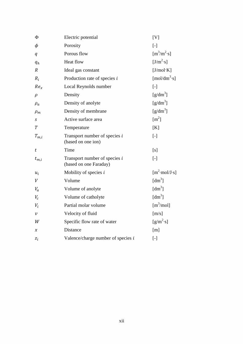
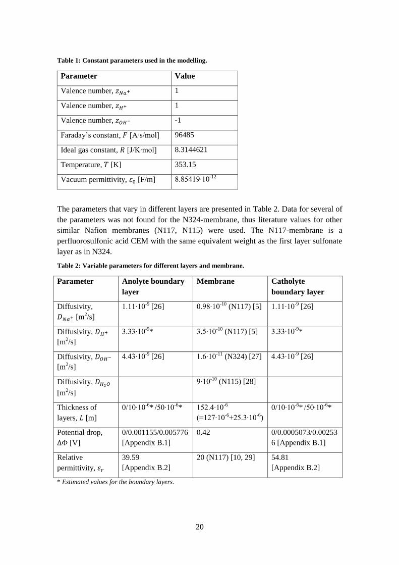
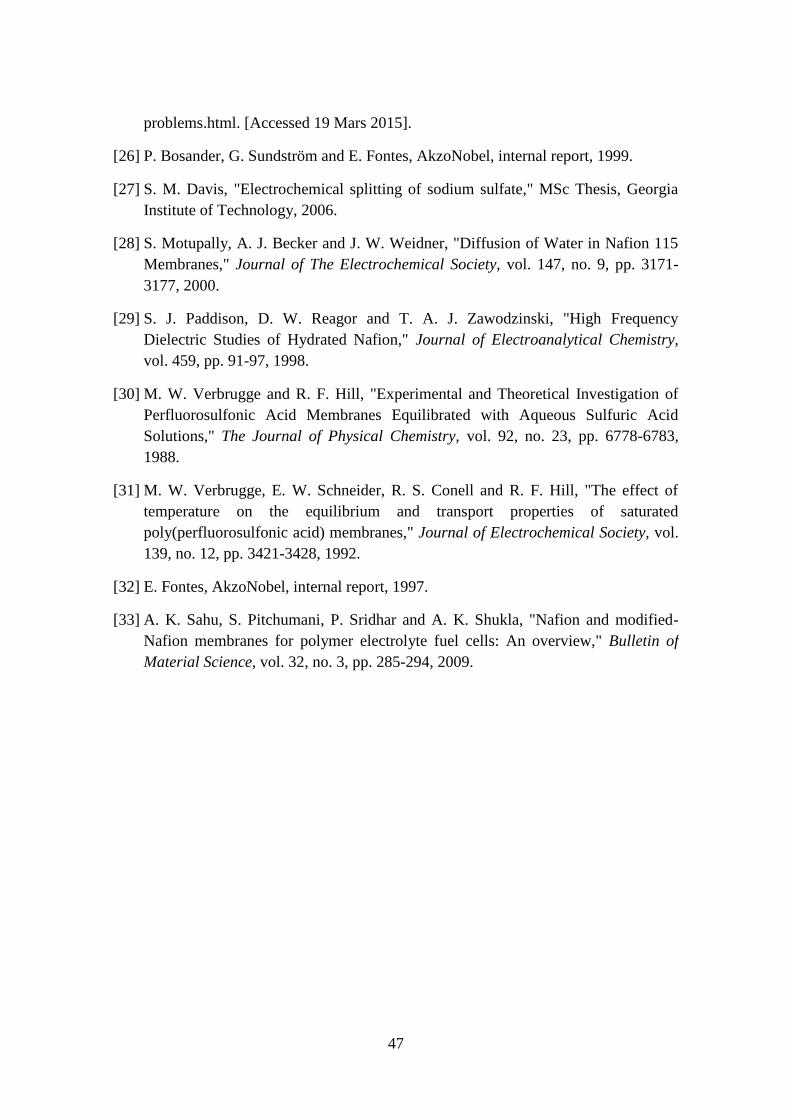
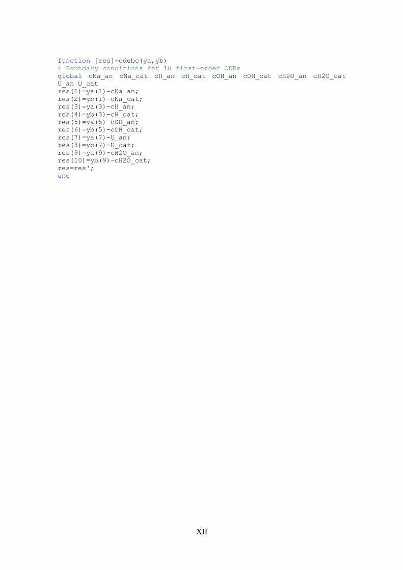
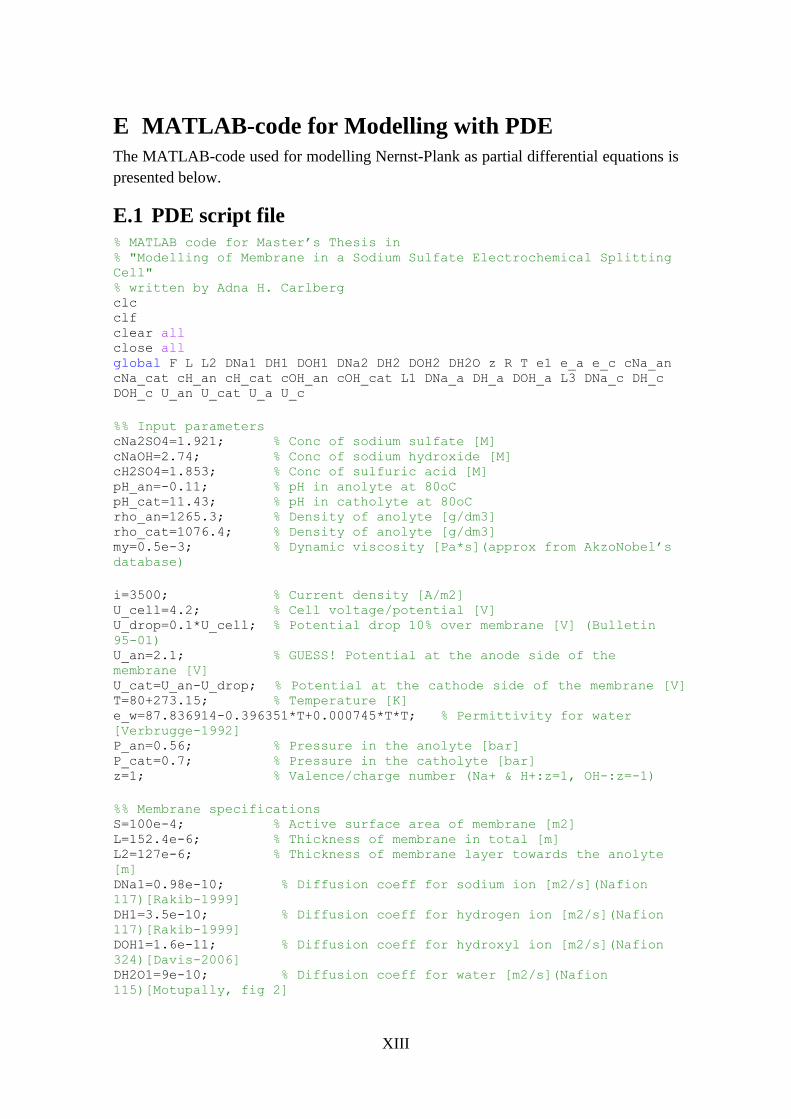
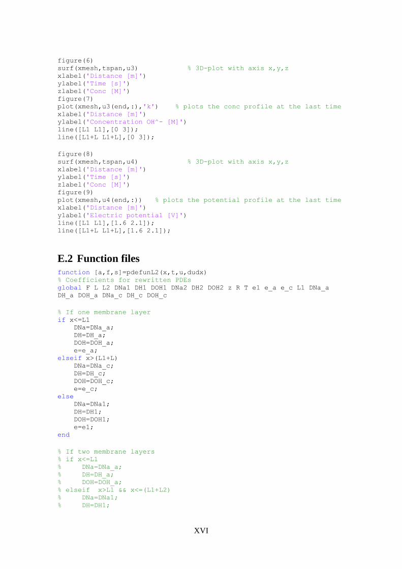

XX
Figure 20 Concentration profile in time and space for hydrogen ions from PDE solution
Figure 21 Concentration profile in time and space for hydroxyl ions from PDE solution