MODELLING OF ANOMALOUS CHARGE CARRIERS … · TRANSPORT IN DISORDERED ORGANIC SEMICONDUCTORS CHOO...

MODELLING OF ANOMALOUS CHARGE CARRIERS

TRANSPORT IN DISORDERED ORGANIC

SEMICONDUCTORS

CHOO KAN YEEP

FACULTY OF SCIENCE

UNIVERSITY OF MALAYA

KUALA LUMPUR

2017

MODELLING OF ANOMALOUS CHARGE

CARRIERS TRANSPORT IN DISORDERED ORGANIC

SEMICONDUCTORS

CHOO KAN YEEP

THESIS SUBMITTED IN FULFILMENT OF THE

REQUIREMENTS FOR THE DEGREE OF DOCTOR OF

PHILOSOPHY

DEPARTMENT OF PHYSICS

FACULTY OF SCIENCE


KUALA LUMPUR

2017

ii


ORIGINAL LITERARY WORK DECLARATION

Name of Candidate: CHOO KAN YEEP

Matric No: SHC100060

Name of Degree: DOCTOR OF PHILOSOPHY

Title of Thesis (“this Work”):

MODELLING OF ANOMALOUS CHARGE CARRIERS TRANSPORT IN

DISORDERED ORGANIC SEMICONDUCTORS

Field of Study:

THEORETICAL PHYSICS

I do solemnly and sincerely declare that:

(1) I am the sole author/writer of this Work;

(2) This Work is original;

(3) Any use of any work in which copyright exists was done by way of fair

dealing and for permitted purposes and any excerpt or extract from, or

reference to or reproduction of any copyright work has been disclosed

expressly and sufficiently and the title of the Work and its authorship have

been acknowledged in this Work;

(4) I do not have any actual knowledge nor do I ought reasonably to know that

the making of this work constitutes an infringement of any copyright work;

(5) I hereby assign all and every rights in the copyright to this Work to the

University of Malaya (“UM”), who henceforth shall be owner of the

copyright in this Work and that any reproduction or use in any form or by any

means whatsoever is prohibited without the written consent of UM having

been first had and obtained;

(6) I am fully aware that if in the course of making this Work I have infringed

any copyright whether intentionally or otherwise, I may be subject to legal

action or any other action as may be determined by UM.

Candidate’s Signature Date:

Subscribed and solemnly declared before,

Witness’s Signature Date:

Name:

Designation:

iii

ABSTRACT

Performance of organic devices is affected by material disorders, which yields low

mobility, dispersive current and scaling noise behaviour. Anomalous transport and

scaling noise behaviour are inadequately described by Fick’s law and characterised by

low-frequency noise method. This work reports the study of (i) scaling behaviour of

current noise in organic field-effect transistors (OFETs) using methods of fractal noise

analysis and, (ii) the modelling of anomalous charge transports in disordered organic

semiconductors based on fractional calculus. Current noises of Poly(3-hexylthiophene)

(P3HT) OFETs were measured at various source-drain voltages (Vds) and characterised

using the power spectral density method and detrended fluctuation analysis. Current

noises were found to follow white noise, 1/f and Brownian noise characteristic at low,

intermediate and high Vds, respectively. For Vds above 40 V, Brownian noise will be

masked out by 1/f noise. Multiple-trapping mechanism is integrated with the drift-

diffusion equation and then generalised to the time-fractional drift-diffusion equation

(TFDDE) to model the anomalous transports and reproduce the transient photocurrents

in regiorandom P3HT (RRa-P3HT) and regioregular P3HT (RR-P3HT). The TFDDE is

solved by using finite difference scheme and Poisson solver is implemented to calculate

the electric field. It is found that by acquiring extra energy from high electric field,

charge carriers escape easily from trap centres and propagate with higher velocity

resulting in higher current. Larger amount of charge carriers will be generated at higher

illumination and they will be hopping near the mobility edges, hence encountering

lesser capturing events. This explains why movement of charge carriers at higher

illumination is less dispersive than the movement of charge carriers at lower

illumination. It is also noted that transport dynamic of charge carriers in RR-P3HT is

relatively less dispersive and has higher mobility than that of the RRa-P3HT since RR-

P3HT has lower capturing rate and is less energetically disordered.

iv

ABSTRAK

Prestasi peranti organik dipengaruhi oleh kecelaruan bahan yang menghasilkan

mobiliti rendah, serakan arus elecktrik dan sifat hingar berskala. Angkutan anomali dan

sifat hingar berskala adalah tidak sesuai diterangkan oleh hukum Fick dan dicirikan oleh

kaedah hingar frekuensi-rendah. Kajian ini bertujuan untuk (i) mengkaji sifat hingar

berskala arus elektrik dalam transistor kesan-medan organik (OFETs) dengan

menggunakan kaedah analisis hingar fraktal dan (ii) untuk permodelan angkutan

anomali dalam semikonduktor organik bercelaru berdasarkan kalkulus pecahan. Hingar

arus elektrik untuk Poly(3-hexylthiophene) (P3HT) OFETs diukur pada pelbagai voltan

salir-sumber (Vds) dan kemudian dianalisiskan dengan kaedah ketumpatan spektra kuasa

dan analisis fluktuasi nyahpola. Hingar arus elektrik yang bersifat putih, 1/f dan Brown

ditunjukkan masing-masing pada Vds rendah, pertengahan dan tinggi. Hingar Brown

akan dihilangkan oleh hingar 1/f untuk Vds yang lebih tinggi dari 40 V. Mekanisme

perangkap berganda disepadukan dengan persamaan resapan-hayutan dan kemudian

diitlakkan ke persamaan resapan-hayutan pecahan masa (PRHPM) untuk memodel

angkutan anomali dan menghasilkan arusfoto elektrik semasa dalam regiorandom P3HT

(RRa-P3HT) dan regioregular P3HT (RR-P3HT). PRHPM diselesaikan dengan kaedah

perbezaan terhingga dan penyelesaian Poisson juga dilaksanakan untuk penghitungan

medan elektrik. Penghasilan arus yang lebih tinggi pada medan elektrik tinggi adalah

disebabkan oleh pembebasan dan perlonjatan pembawa cas dari pusat perangkap yang

lebih mudah. Pergerakan pembawa cas pada pencahayaan tinggi adalah kurang terserak

kerana cas melompat berhampiran pinggiran mobiliti dengan menghadapi perangkapan

yang lebih kecil. Selain itu, dinamik angkutan pembawa cas dalam RR-P3HT adalah

kurang terserak dan mempunyai mobiliti lebih tinggi dari RRa-P3HT kerana RR-P3HT

mempunyai kadar perangkapan yang lebih rendah dan kurang tenaga bercelaru.

v

ACKNOWLEDGEMENTS

First and foremost, I would like to express my sincere gratitude to my supervisors

Prof. Dr. Sithi V. Muniandy and Dr. Woon Kai Lin for their continuous knowledge

sharing, motivation, encouragement and support given to me during my study.

I would like to thank Dr. C. L. Chua for his help in fabrication of OFET and current-

voltage measurements. I would also like to thank Mr. Gan Ming Tao for his precious

time spent in several detailed discussions about the mathematical techniques required in

my works.

In particular, I am deeply grateful to Dr. Renat T. Sibatov for his kindness and

precious times spent in numerous discussions on the anomalous transport theory in

disordered materials. I am also very grateful to Dr. Frédéric Laquai (Max Planck

Institute for Polymer Research, Germany) for providing me the detailed information on

the device parameters and experiment conditions of the time-of-flight measurements

published in his works.

Last but not least, my sincere thanks go to my parents, siblings and friends who have

been consistently supporting me throughout the journey of my study and thesis writing.

vi

TABLE OF CONTENTS

Abstract ........................................................................................................................... iii

Abstrak ............................................................................................................................ iv

Acknowledgements .......................................................................................................... v

Table of Contents ........................................................................................................... vi

List of Figures ................................................................................................................. ix

List of Tables ................................................................................................................ xiii

List of Symbols and Abbreviations ............................................................................. xiv

List of Appendices ........................................................................................................ xxi

CHAPTER 1: INTRODUCTION .................................................................................. 1

1.1 Prospects and challenges in organic electronics ...................................................... 1

1.2 Motivation and Objectives ....................................................................................... 6

1.3 Organisation of thesis .............................................................................................. 7

CHAPTER 2: LITERATURE REVIEW AND BACKGROUND THEORY ........... 9

2.1 Materials for organic electronics ............................................................................. 9

2.2 Operation of field-effect transistor ........................................................................ 14

2.3 Performance limiting factors of transistors............................................................ 16

2.3.1 Noises in organic field-effect transistor ................................................... 17

2.3.2 Dispersive current and low mobility ........................................................ 21

2.4 Charge transport theories for OFET ...................................................................... 25

2.5 Fractal theory ......................................................................................................... 31

2.5.1 Fractal modelling of signals and surfaces ................................................ 45

2.5.2 Fractal dynamics ....................................................................................... 50

2.6 Normal diffusion theory for charge transport in ordered material ........................ 52

vii

2.7 Fractional calculus theory ...................................................................................... 58

2.8 Theories of anomalous charge transport ................................................................ 61

2.8.1 Time-of-flight measurement ..................................................................... 62

2.8.2 Continuous-time random walk theory ...................................................... 65

CHAPTER 3: RESEARCH METHODOLOGY ....................................................... 76

3.1 Fabrication of organic field-effect transistor and current-voltage measurement ... 76

3.2 Low-frequency noise measurement ....................................................................... 78

3.3 Fractal analysis of current noise ............................................................................ 81

3.3.1 Power spectral density method ................................................................. 81

3.3.2 Detrended fluctuation analysis ................................................................. 82

3.4 Transport equation based on fractional calculus ................................................... 84

3.4.1 Fractional kinetic equation with multiple-trapping mechanism ............... 84

3.4.2 Electric potential and field ....................................................................... 88

3.4.3 Current density ......................................................................................... 88

3.5 Numerical methods ................................................................................................ 89

3.5.1 Finite difference scheme for integer order differential operator .............. 89

3.5.2 Finite difference scheme for fractional order differential operator .......... 90

3.5.3 Numerical integration ............................................................................... 91

3.5.4 Discretisation for partial differential equation ......................................... 94

3.5.5 Gaussian elimination for solving linear equation systems ....................... 96

3.5.6 Discretisation for fractional drift-diffusion equation ............................... 98

3.5.7 Discretisation for electric potential and Poisson equation ..................... 101

3.5.8 Discretisation for current density ........................................................... 103

3.6 Simulation procedures ......................................................................................... 103

viii

CHAPTER 4: OFET NOISE STUDY BASED ON FRACTAL ANALYSIS ........ 106

4.1 Experiment conditions ......................................................................................... 106

4.2 Results and discussion on OFET noise analysis .................................................. 106

4.3 Summary .............................................................................................................. 113

CHAPTER 5: TRANSPORT STUDY OF RRA-P3HT AND RR-P3HT ............... 114

5.1 Simulation conditions .......................................................................................... 114

5.2 Results and discussion on transport dynamics of RRa-P3HT and RR-P3HT ..... 116

5.3 Summary .............................................................................................................. 122

CHAPTER 6: CONCLUSIONS................................................................................. 123

6.1 Summary .............................................................................................................. 123

6.2 Recommendation and future works ..................................................................... 125

References .................................................................................................................... 127

List of Publications and Papers Presented ............................................................... 138

Appendix A – Derivation of transient current density ............................................ 143

Appendix B – Programming code developed for anomalous charge transport .... 145

Appendix C – Stability test and convergence analysis ............................................. 157

ix

LIST OF FIGURES

Figure 1.1: Green electronics: biodegradable and biocompatible materials and

devices for sustainable future. (Irimia-Vladu, 2014)..........................

2

Figure 1.2: Partial market forecast by component type in US$ billion predicted

by IDTechEx. (Das, 2017)..................................................................

3

Figure 1.3: Progress on efficiency of polymer-polymer based solar cell.

(Benten et al., 2016)............................................................................

4

Figure 1.4: Progress in mobility improvement for p-type and n-type OFETs.

(Dong et al., 2010)...............................................................................

5

Figure 1.5: 8-bit, 6 Hz plastic microprocessor made of 3381 pentacene

transistors fabricated on a plastic foil. (Myny et al., 2012).................

6

Figure 2.1: (a) Very thin pentacene single crystals deposited on a SiO2/Si

substrate, (b) Copper grid is used as mask to complete fabrication of

the OFETs. (Dong et al., 2016)...........................................................

10

Figure 2.2: Examples of P3HT di-block copolymers. (Bhatt et al., 2014)............ 11

Figure 2.3: (a) Structure and (b) molecular arrangement of Cn-BTBT. (Ebata et

al., 2007)..............................................................................................

13

Figure 2.4: (a) Molecular and (b) single structure of N,N′-

bis(cyclohexyl)naphthalene diimide. (Shukla et al., 2008).................

14

Figure 2.5: (a) Top-contact and (b) bottom-contact configurations of OFET.

(Shirota & Kageyama, 2007)..............................................................

15

Figure 2.6: Current-voltage characteristic of an OFET for increasing Vg from

(a) to (e). (Shirota & Kageyama, 2007)..............................................

16

Figure 2.7: Normalised noise power spectra of undoped amorphous silicon at

four temperature (i) 495 K, (ii) 483 K, 467 K and (iv) 454 K.

(Johanson et al., 2002).........................................................................

18

Figure 2.8: Noise power spectra for various III-V semiconductor heterojunction

bipolar transistors. (Pénarier et al., 2002)...........................................

19

Figure 2.9: Low-frequency noise power spectra density for HMDS treated RR-

P3HT OFET. (Ke et al., 2008)............................................................

20

Figure 2.10: (a) Non-dispersive and (b) dispersive transient photocurrents.

(Shirota & Kageyama, 2007)..............................................................

22

Figure 2.11: Schematic diagram for SHG measurement. (Manaka et al., 2006)..... 24

Figure 2.12: Schematic diagram showing the distribution of transport sites in (a)

space, (b) energy and (c) two dimensional map of energy surface.

(Tessler et al., 2009)............................................................................

26

x

Figure 2.13: Sierpinski triangle. (Fractal organisation)........................................... 33

Figure 2.14: (a) von Koch curve at different level of magnification and (b) von

Koch snowflake. (Falconer, 1990)......................................................

34

Figure 2.15: Radially linked star-block-linear polystyrene polymers. (Knauss &

Huang, 2003).......................................................................................

35

Figure 2.16: Julia set. (McMullen, 1998)................................................................ 35

Figure 2.17: Romanesco broccoli at different magnification levels. (King, 2016). 36

Figure 2.18: Fern leaf decomposed to four magnification levels............................ 37

Figure 2.19: Barnsley fern generated by IFS method. (Barnsley, 1993)................. 38

Figure 2.20: The environment dependence of growth morphology of Physarum

Polycephalum plasmodium. (Takamatsu et al., 2009)........................

39

Figure 2.21: Mandelbrot set. (Falconer, 1990)........................................................ 40

Figure 2.22: Coastline of Great Britain. (“Geometric Fractal - Chapter 2 Fractal

Dimension of Coastlines”)..................................................................

41

Figure 2.23: Weierstrass function at (a) H = 0.1, (b) H = 0.3, (c) H = 0.5, and (d)

H = 0.7. (Canus et al., 2003)...............................................................

42

Figure 2.24: Displacement of three particles recorded in the experiment

conducted by Perrin. (Perrin et al., 1910)...........................................

43

Figure 2.25: Brownian motion simulated at various step intervals. (Turner et al.,

1998)....................................................................................................

44

Figure 2.26: Brownian function, H = 0.5, at various magnification levels. (Canus

et al., 2003)..........................................................................................

45

Figure 2.27: Fractional Brownian motion at various H values. (Canus et al.,

2003)....................................................................................................

46

Figure 2.28: Fractional Brownian surfaces for (a) H = 0.1, (b) H = 0.3, (c) H =

0.5 and (d) H = 0.7. (Canus et al., 2003).............................................

48

Figure 2.29: Gradient percolation of atoms with diffusion length LD = 10240 on

a 512512 lattice. (Wool & Long, 1993)............................................

49

Figure 2.30: A basic setup for a TOF measurement. (Scher & Montroll, 1975)..... 62

Figure 2.31: Step-like and dispersive current pulses obtained from TOF

measurement. The step-like transient current indicates a packet of

charge carriers is drifting with a constant velocity until it leaves the

DUT at transit time..............................................................................

63

Figure 2.32: A double-log plot of transient photocurrent associated with a packet

of charge carriers moving in an electric field, with a hopping-time

distribution function (t) ~ t-1-

, 0 < < 1, towards an absorbing

xi

barrier at the sample surface. (Scher & Montroll, 1975).................... 65

Figure 2.33: Comparison between the trajectories of Brownian motion (left) and

Lévy flight at Df = 1.5 (right) for about 7000 steps. (Metzler &

Klafter, 2000c)....................................................................................

71

Figure 3.1: Top-contact and bottom-gate P3HT OFET structure and setup of

current-voltage measurement..............................................................

77

Figure 3.2: System for measuring low-frequency noise. (Kasap & Capper,

2006)....................................................................................................

78

Figure 3.3: 1/f noise spectra due to cumulative sum of generation-

recombination noise. (Kasap & Capper, 2006)...................................

79

Figure 3.4: Current noise analysis based on PSD method and DFA..................... 80

Figure 3.5: Detrending procedure of DFA at different window sizes. (Penzel et

al., 2003)..............................................................................................

83

Figure 3.6: Double-log plot for r.m.s. fluctuation F versus box size. (Penzel et

al., 2003)..............................................................................................

84

Figure 3.7: Comparison between the Trapezoid Rule and Simpson's Rule.

(Cheney & Kincaid, 2008)..................................................................

92

Figure 3.8: Implicit difference scheme for diffusion equation.............................. 95

Figure 3.9: Flow chart of transport dynamic simulation of charge carrier............ 104

Figure 3.10: Transient currents calculated for various mesh sizes.......................... 105

Figure 4.1: Output characteristic of P3HT OFET with channel length of 40 m.

The source-drain voltage is swept from 0 V to 60 V for each gate

voltage.................................................................................................

106

Figure 4.2: Measured transient current noises of OFETs at various Vds: (a) 1

V, (b) 10 V, (c) 20 V, (d) 25 V and (e) 50 V..............................

107

Figure 4.3: PSDs of transient current noises of OFETs obtained at various Vds:

(a) 1 V, (b) 10 V, (c) 20 V, (d) 25 V and (e) 50 V. The

straight line indicates the least-squares line of the PSD......................

109

Figure 4.4: DFA of transient current noises of OFETs obtained at various Vds:

(a) 1 V, (b) 10 V, (c) 20 V, (d) 25 V and (e) 50 V. The

straight line indicates the least-squares line of the DFA.....................

110

Figure 5.1: Schematic diagram represents the cell in TOF measurement............. 114

Figure 5.2: Transient current curves: symbols (digitised from Figure 6 in

(Mauer et al., 2010)) - TOF measurement data for RRa-P3HT at

different electric fields; lines: simulated results using the VO-

TFDDE at different electric fields.......................................................

117

xii

Figure 5.3: Charge carrier density profile for RRa-P3HT at various electric

fields and times....................................................................................

118

Figure 5.4: Transient current curves: symbols (digitised from Figure 2 in

(Mauer et al., 2010)) - TOF measurement data for RR-P3HT

(~94%) at different light intensities; lines - simulated results using

the VO-TFDDE at different electric fields..........................................

119

Figure 5.5: Generation and propagation of charge carries at low light intensity... 119

Figure 5.6: Charge carrier density profile for RR-P3HT (~94%) at various

times for (a) low-light intensity and (b) high-light intensity...............

120

Figure 5.7: Generation and propagation of charge carries at high light intensity. 121

xiii

LIST OF TABLES

Table 5.1: Simulation parameters for RRa-P3HT. ........................................................ 115

Table 5.2: Simulation parameters for RR-P3HT (~94%). ............................................ 116

xiv

LIST OF SYMBOLS AND ABBREVIATIONS

AlGaAs : Aluminium gallium arsenide

C10-DNTT : 2,9-di-decyl-dinaphtho-[2,3-b:20,30-f]-thieno-[3,2-b]-thiophene

C8-BTBT : 2,7-dioctyl[1]benzothieno[3,2-b][1]benzothiophene

CELIV : Charge extraction by linearly increasing voltage

Cn-BTBT : 2,7-dialkyl[1]benzothieno[3,2-b][1]-benzothiophene

CP : Caputo

CTRW : Continuous-time random walk

DDE : Drift-diffusion equation

DE : Diffusion equation

DFA : Detrended fluctuation analysis

DLA : Diffusion-limited aggregation

DMM : Digital multimeter

DOS : Density of states

DSA : Dynamic signal analyser

DUT : Device under test

FBM : Fractional Brownian motion

FDDE : Fractional drift-diffusion equation

FDE : Fractional diffusion equation

FET : Field-effect transistor

FFPE : Fractional Fokker-Planck equation

FFT : Fast Fourier transform

FKKE : Fractional Klein-Kramer equation

FLE : Fractional Langevin equation

FPE : Fokker-Planck equation

xv

GaAs : Gallium arsenide

GaInP : Gallium indium phosphide

GDM : Gaussian disorder model

GL : Grüwald-Letnikov

GLE : Generalised Langevin equation

HBT : Heterojunction bipolar transistors

HMDS : Hexamethyldisilazane

IFS : Iterated function system

InGaAs : Indium gallium arsenide

InP : Indium phosphide

KCl : Potassium chloride

L.H.S. : Left hand side

LE : Langevin equation

LFN : Low-frequency noise

MATR : Miller-Abrahams transition rate

MSD : Mean squared displacement

MTR : Marcus transition rate

MVRHM : Mott variable range hopping model

NDI : Naphthalene diimide

OFET : Organic field-effect transistor

OLED : Organic light-emitting diode

OSC : Organic solar cell

OSK : Oscilloscope

OTFT : Organic thin-film transistor

OTS : Octadecyl triethoxysilane

P3HT : Poly(3-hexylthiophene)

xvi

PBI : Perylene Bisimide

PCE : Power conversion efficiency

PDE : Partial differential equation

PDF : Probability density function

PDVT :

Poly[2,5-bis(alkyl)pyrrolo[3,4-c]pyrrole-1,4(2H,5H)-dione-alt-5,5′-

di(thiophen-2-yl)-2,2′-(E)-2-(2-(thiophen-2-yl)vinyl)thiophene]

PSA : Power spectrum analyser

PSD : Power spectral density

R.H.S. : Right hand side

r.m.s. : Root mean square

RL : Riemann-Liouville

RRa-P3HT : Regiorandom poly(3-hexylthiophene)

RR-P3HT : Regioregular poly(3-hexylthiophene)

RTS : Random telegraph signal

S/N : Signal-to-noise

SHG : Optical second-harmonics-generation

SiO2 : Silicon dioxide

SMU : Source-measurement unit

TFDDE : Time-fractional drift-diffusion equation

TOF : Time-of-flight

TFT Thin-film transistor

VO-TFDDE : Variable-order time-fractional drift-diffusion equation

1 2,HB t

C t t : Covariance of BH(t)

0

RL

tD : RL factional derivative operator of order

0

C

tD : Caputo factional derivative operator of order

xvii

W

tD

: Weyl factional derivative operator of order

0

RL

tD : RL factional integral operator of order

0

C

tD : Caputo factional integral operator of order

W

tD

: Weyl factional integral operator of order

a tD or

t

: Factional derivative operator of order

a tD or

t

: Factional integral operator of order

: Mobility

: Friction constant

: Disorder parameter or fractional derivative order

() : Gamma function with real argument

(k) : Fourier transform of (x)

(t) : Cumulative jump probability within (0,t)

(x) : Jump length PDF

(x)(t) : Initial condition of random walker

(x,t) : Disorder parameter or fractional derivative order in space and time

(x,t) : Charge density

0 : Average time of delocalisation

0 : Capture rate of charge carrier into the localised state

0 : Permittivity of vacuum

2 : Laplace transform of spatial step

c : Characteristic waiting time

xviii

D : Deep trapping lifetime

DFA : Scaling exponent for DFA

PS : Scaling exponent of PSD

r : Relative permittivity of material

rc : RC time constant

t : Time interval

x : Space interval

1/f : Flicker noise

BH(t) : Fractional Brownian motion

c : Charge carrier capture coefficient

c(x,t) : Concentration of particle

Ci : Capacitance

D : Diffusion coefficient

D : Anomalous diffusion coefficient

DB : Box dimension

Df : Fractal dimension

DH : Hausdorff dimension

e : Electronic charge

E[BH(t)] : Mean of BH(t)

E0 : Mean value of the exponential energy DOS of charge carrier

f : Frequency

F(x) : External force

f(x,t) : Function of space x and time t

H : Hurst exponent

i : Space index

xix

IT(t) : Average current density

j(x,t) : Flow current density

k : Time index

K : Anomalous diffusion constant

K(x,t) : Anomalous advection coefficient at x and t

kB : Boltzmann constant

L : Device length

ld : Average length of delocalisation

m : Mass of particle

N : Total number of particles

n(x',t') : PDF just arrived at position x' at time t'

p(x,0)(t) : Initial photo-generated charge carriers

p(x,t) : Total charge carrier density at x and t

pf(x,t) : Sum of free charge carrier density at x and t

pt(x,t) : Sum of trap charge carrier density at x and t

r1 : Transition probability of flow to right

r2 : Transition probability of flow to left

s : Time variable

S(f) : Power spectral density

t : Time variable

T : Temperature

ttr : Transit time

v(x) : Velocity

V(x) : Applied potential

Va : Applied bias

Var[BH(t)] : Variance of BH(t)

xx

Vds : Source-drain voltage

Vg : Gate voltage

Vs : Source voltage

Vth : Threshold voltage

W(k,u) : Fourier-Laplace of W(x,t)

w(t) : Waiting time PDF

w(u) : Laplace transform of w(t)

W(x,t) : PDF of being in x at time t

W0(k) : Fourier transform of W0(x)

W0(x) : Initial condition of W(x,t)

x : Position in one-dimensional Cartesian-coordinate space

Y(j) : Integrated time series

Σ2 : Jump length variance

xxi

LIST OF APPENDICES

Appendix A – Derivation of transient current density............................................... 143

Appendix B – Programming code developed for anomalous transport..................... 145

Appendix C – Stability test and convergence analysis.............................................. 157

1

CHAPTER 1: INTRODUCTION

A brief overview on the prospects and challenges faced in organic electronics is

provided in this chapter together with the motivation and objectives of this work.

Besides, the outline of the thesis is also presented at the end of this chapter.

1.1 Prospects and challenges in organic electronics

Since the first conducting polymer reported in 1970’s (Heeger et al., 2002), organic

semiconductor and polymer materials have drawn tremendous research and also

industry attentions due to their several key advantages, namely: (i) low temperature and

relatively simple processing yield energy-efficient production and reduction in

manufacturing cost, (ii) versatility of synthesis processes which facilitate the production

of enormous choices of engineered organic semiconductors and polymer materials for

enhancement in mobility, light conversion efficiency, temperature resistance and long

term stability, (iii) well-matched on a wide range of flexible plastic substrates and

transparent glasses and (iv) continuous improvement on large-area printing technique

which allows high throughput production of organic semiconductor and polymer

devices.

Owing to the above mentioned advantages, organic semiconductors and polymers

have become very promising choices of materials for realisation of flexible display and

lighting technologies, large-area printable optoelectronic devices for energy harvesting,

flexible and wearable electronic and optoelectronic devices and organic sensors, which

are fabricated based on organic light-emitting diodes (Ho et al., 2015), organic solar

cells (Milichko et al., 2016) and organic field-effect transistors (Sirringhaus, 2014).

Anticipating the coming of new applications of OLEDs and OFETs is certainly

tempting, and has been envisioned in Figure 1.1. Besides, there are also research

interests branching into production of green materials and devices that possess human

2

and environmentally friendly features, including biodegradability and biocompatible

(Irimia-Vladu, 2014).

Figure 1.1: Green electronics: biodegradable and biocompatible materials and devices

for sustainable future. (Irimia-Vladu, 2014)

IDTechEx forecasted that investments in producing cheap and high performance

organic semiconductor or polymer-based optoelectronic and electronic devices will be

continuously growing and generating a market worth of US$70 billion in 2027 from the

current market value of US$29 billion in 2017. As shown in Figure 1.2, the main

contributors to the total market worth are due to OLEDs and conductive ink. In

additions, a great potential market growth is expected for flexible electronics, logic and

memory, and thin film sensors due to the advancement in research and development

(Das, 2017).

3

Figure 1.2: Partial market forecast by component type in US$ billion predicted by

IDTechEx. (Das, 2017)

Organic and polymer-based solar cells are among the potential candidates for

realisation of green optoelectronic devices as they can be printed on either a large-area

flexible or a glass substrate for solar energy harvesting and electricity generation

(Mazzio & Luscombe, 2015; Sekine et al., 2014). For instance, solar energy could be

harvested by the OSCs when they are printed on the windows of a building or a small

panel on a wearable device. Due to the huge investments and intense collaborations

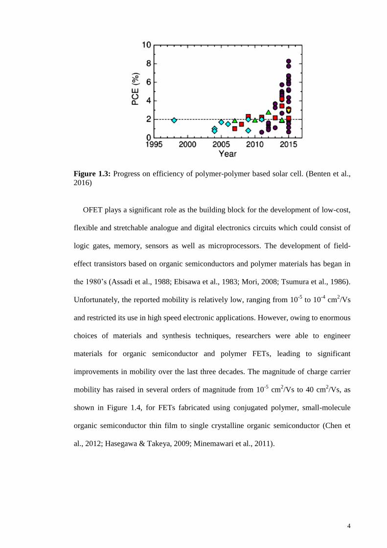
between governments, industrial partners and researchers, the power conversion

efficiency of polymer based solar cells has significantly increased from roughly 2% in

2010 to slightly beyond 8% in 2015 as depicted in Figure 1.3 (Benten et al., 2016).

These solar cells are fabricated using conjugated polymers which act as the electron

donor and acceptor and also enhance the flexibility and mechanical properties of the

device as compared to that of the solar cell based on polymer-fullerene blend.

4

Figure 1.3: Progress on efficiency of polymer-polymer based solar cell. (Benten et al.,

2016)

OFET plays a significant role as the building block for the development of low-cost,

flexible and stretchable analogue and digital electronics circuits which could consist of

logic gates, memory, sensors as well as microprocessors. The development of field-

effect transistors based on organic semiconductors and polymer materials has began in

the 1980’s (Assadi et al., 1988; Ebisawa et al., 1983; Mori, 2008; Tsumura et al., 1986).

Unfortunately, the reported mobility is relatively low, ranging from 10-5

to 10-4

cm2/Vs

and restricted its use in high speed electronic applications. However, owing to enormous

choices of materials and synthesis techniques, researchers were able to engineer

materials for organic semiconductor and polymer FETs, leading to significant

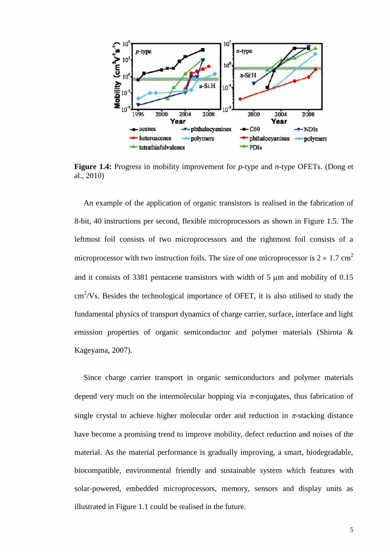
improvements in mobility over the last three decades. The magnitude of charge carrier

mobility has raised in several orders of magnitude from 10-5

cm2/Vs to 40 cm

2/Vs, as

shown in Figure 1.4, for FETs fabricated using conjugated polymer, small-molecule

organic semiconductor thin film to single crystalline organic semiconductor (Chen et

al., 2012; Hasegawa & Takeya, 2009; Minemawari et al., 2011).

5

Figure 1.4: Progress in mobility improvement for p-type and n-type OFETs. (Dong et

al., 2010)

An example of the application of organic transistors is realised in the fabrication of

8-bit, 40 instructions per second, flexible microprocessors as shown in Figure 1.5. The

leftmost foil consists of two microprocessors and the rightmost foil consists of a

microprocessor with two instruction foils. The size of one microprocessor is 2 1.7 cm2

and it consists of 3381 pentacene transistors with width of 5 m and mobility of 0.15

cm2/Vs. Besides the technological importance of OFET, it is also utilised to study the

fundamental physics of transport dynamics of charge carrier, surface, interface and light

emission properties of organic semiconductor and polymer materials (Shirota &

Kageyama, 2007).

Since charge carrier transport in organic semiconductors and polymer materials

depend very much on the intermolecular hopping via -conjugates, thus fabrication of

single crystal to achieve higher molecular order and reduction in -stacking distance

have become a promising trend to improve mobility, defect reduction and noises of the

material. As the material performance is gradually improving, a smart, biodegradable,

biocompatible, environmental friendly and sustainable system which features with

solar-powered, embedded microprocessors, memory, sensors and display units as

illustrated in Figure 1.1 could be realised in the future.

6

Figure 1.5: 8-bit, 6 Hz plastic microprocessor made of 3381 pentacene transistors

fabricated on a plastic foil. (Myny et al., 2012)

1.2 Motivation and Objectives

Disorderness in organic semiconductor and polymer causes low mobility and

fluctuation in number of charge carriers which lead to low speed, low bandwidth, high

noise floor and low signal-to-noise ratio. These unwanted effects eventually degrade the

device performance and limit its applications. Disordered properties in organic

semiconductor and polymer may also be reflected in current noise spectra as it has a

tendency to deviate from the typical 1/f noise characteristics and led to anomalous

charge transport with long-current tail. It has been known that the multi-scaling current

noise and anomalous transport behaviour are inadequately described by the

conventional 1/f type spectral interpretation and Fick's diffusion law, respectively. On

the other hand, it has been demonstrated that fractal analysis is useful for analysing

nonstationary signal and it is rather tempting to explore its application in studying

scaling behaviour of current noise in OFET. Likewise, fractional calculus has found

many applications in the modelling of complex phenomena with nonlocal effects,

namely long memory and long range dependence. Almost every dynamical equation

7

known in the fields of physical science have been reformulated using fractional

differential/integral operators. Thus, it is once again obvious to generalise the Fick’s

diffusion equation to the fractional drift-diffusion equation to model the anomalous

transport dynamics in disordered material. While the theoretical formulations are robust

and intuitive, analytical solution to time-fractional drift-diffusion equation is not always

possible in most general cases. One has ultimately resort to numerical solutions with

efficient algorithms that could handle and optimise non-local differential operators. In

this study, the focus will also be on the understanding of the origins of the scaling

behaviours of current noise in OFETs, the causes of long-tail transient currents and the

suitability of fractional drift-diffusion equation for modelling of charge carrier transport

in disordered organic semiconductors. Therefore the objectives of this study are:

1. to analyse the scaling behaviours of current noise in P3HT OFET using fractal noise

theory.

2. to relate the scaling behaviours of current noise to the charge carriers transport

mechanisms through the spectra and scaling exponents.

3. to study the anomalous charge carriers transport dynamics in disordered organic

semiconductors at different fields and light intensities.

4. to develop a phenomenological model which is capable of describing the normal and

anomalous charge carrier transports based on fractional differential equation.

1.3 Organisation of thesis

Chapter 1 provides a brief overview and challenges on organic electronics that are

relevant to the present work, especially in defining the motivation and the objectives of

this study. Literature review is provided in Chapter 2. Brief description on the

background theory is included here to lead the reader to the related concepts and tools

required in this work. An overview about organic semiconductors and polymers,

8

operations and noises in the field-effect transistors, fractal modelling of signals, surfaces

and transport dynamics are given in this chapter. Several normal and anomalous

transport theories are presented in this chapter. Chapter 2 also introduces the fractional

calculus theory, which serves as the mathematical framework for the derivation of

anomalous transport model for disordered material. The fabrication and characterisation

of OFET, low-frequency noise measurement and fractal analysis techniques are

demonstrated in the first half of Chapter 3. The second part of this chapter continues

with the derivation of the anomalous transport equation incorporated with multiple-

trapping using fractional calculus, the numerical methods required to solve the

fractional drift-diffusion equation and ends with the simulation procedures. Chapter 4

begins with a summary of the measurement conditions of P3HT OFET and then

followed by the discussion on the scaling behaviours of current noise subjected to the

presence of trap centres at different applied source-drain voltage. The simulation

conditions for modelling the charge transport in RR-P3HT and RRa-P3HT materials are

given in the beginning of Chapter 5 and then ended with the discussions on the transport

dynamics of RRa-P3HT at various applied bias and RR-P3HT at different light intensity

levels. Conclusions of this work, recommendations and suggestions for future work are

reported in Chapter 6.

9

CHAPTER 2: LITERATURE REVIEW AND BACKGROUND THEORY

Chapter 2 begins with a brief overview on the development of materials for plastic

electronics, followed by the operation, performance limiting factors and charge

transport theory of OFETs. Description on the fractal theory is given because it serves

as the fundamental concept for current noise analysis. Several charge transport theories

based on normal diffusion process are presented because they are commonly used to

model charge transport in crystalline material. Besides, these models can be generalised

to describe the anomalous charge transport in disordered materials using fractional

calculus. Lastly, the details of the anomalous transport models are given in the last

section of this chapter.

2.1 Materials for organic electronics

Organic semiconductors and polymers used for the fabrication of plastic electronics

could be classified into conjugated polymers, hybrid organic-inorganic structures,

molecular semiconductors, small molecule semiconductors and single crystal structure

polymers. Transistors which are fabricated using the latter two structures have

demonstrated high mobility values exceeding the mobility of amorphous silicon and is

comparable to the mobility of polysilicon.

Pentacene is one of the important polymers that has been extensively studied and

used in the fabrication of OFET. This is simply due to the mobility of pentacene is

matching up to the mobility of amorphous semiconductors. Günther and co-workers had

demonstrated that the mobility of pentacene OFET could achieve a value up to 0.45

cm2/Vs (Günther et al., 2015). They also found out that the mobility of the pentacene

OFET would be reduced when the deposition rate is increased. This is because a larger

amount of grain boundaries is induced in the channel region and hinders the movement

of charge carriers leaving the device. Dong and co-workers (Dong et al., 2016) utilised a

10

very thin single crystal pentacene OFET as shown in Figure 2.1 to achieve the highest

mobility of 5.7 cm2/Vs among pentacene OFETs. The thin layer of single crystal

pentacene was grown from a seed crystal directly on a bare silicone dioxide substrate

using the physical vapour transport method. Thus, pentacene molecules were aligned

themselves orderly to form a monolayer crystal on the SiO2 substrate. This significantly

enhanced the diffusion of charge carries in the single crystal structure and yielded very

high mobility.

(b)

Figure 2.1: (a) Very thin pentacene single crystals deposited on a SiO2/Si substrate, (b)

Copper grid is used as mask to complete fabrication of the OFETs. (Dong et al., 2016)

Besides pentacene, poly(3-hexylthiophene) is also one of the extensively studied

semiconducting conjugated polymers for electronic and optoelectronic applications due

to its exceptional properties such as high mobility, solution-based processability and

thermal properties (Bhatt et al., 2014; Dang et al., 2011). It has been demonstrated that

the performance of P3HT polymer is greatly influenced by its backbone couplings

which result in various types of regioisomers and the molecular weight. Regioregular

P3HT is produced if the entire polymer consists of only the monomers with head-to-tail

coupling configuration and less structural defects. On the other hand, regiorandom

P3HT could have the various types of coupling configurations (Loewe et al., 1999;

Terje & Reynolds, 2006) and Figure 2.2 shows some of the P3HT di-block copolymers.

11

Figure 2.2: Examples of P3HT di-block copolymers. (Bhatt et al., 2014)

It had been shown that RR-P3HT has higher mobility than the mobility of RRa-

P3HT (Mauer et al., 2010). The high mobility achieved for P3HT is 0.4 cm2/Vs which

was measured from the RR-P3HT FETs (Baeg et al., 2010). Although the mobility

demonstrated so far for P3HT OFET has significantly improved, but it is still not

suitable for high-speed device applications which are made from semiconductor

materials. Recently, Nawaz and co-workers reported the highest mobility of 1.2 cm2/Vs

which was measured from the defect free regioregular poly(3-hexylthiophene-2,5-diyl)

OFET (Nawaz et al., 2016). Besides, mobility ranging from 2 to 8.2 cm2/Vs produced

from PDVT-based OFET has been reported (Chen et al., 2012). The reduction in the

distance between the -stacking has tremendously improved the mobility of the P3HT-

based OFET from 10-5

cm2/Vs to 8 cm

2/Vs.

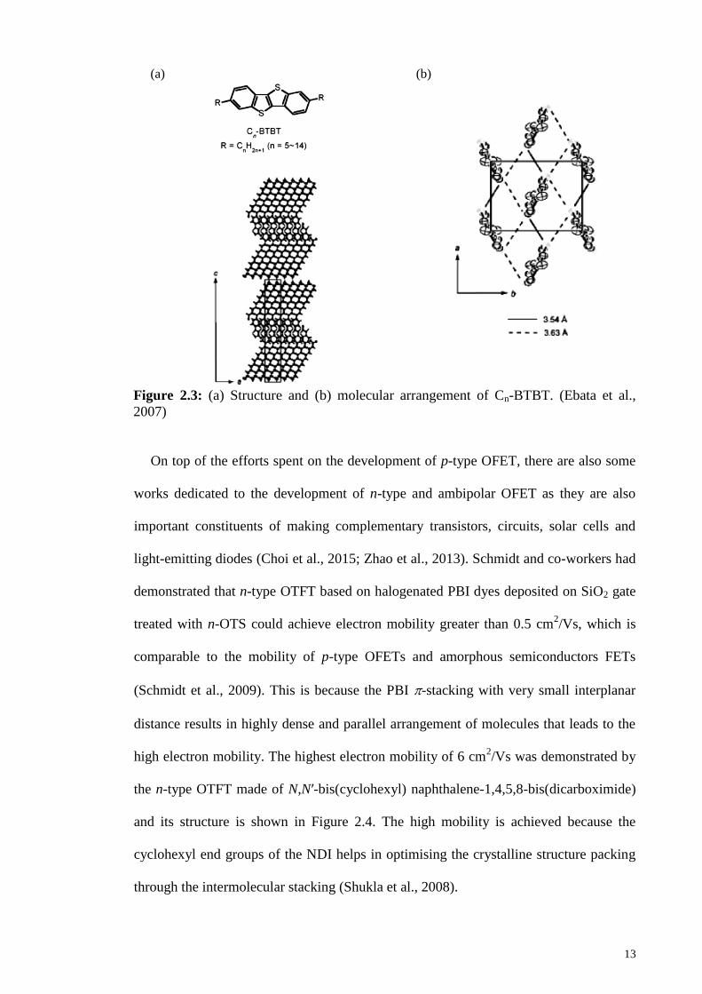
Single crystal structure polymers have been extensively studied in recent years due to

its high-order alignment of molecules and high mobility. Figure 2.3 shows a crystal

structure and molecular arrangement of the single crystal Cn-BTBT derivatives which

were produced by using the Friedel-Crafts acylation and Wolff-Kishner reduction

techniques with BTBT serving as the starting material. The mobility of the BTBT

derivatives was reported to be ranging from 0.16 to 2.75 cm2/Vs for 5 n 14 (Ebata et

12

al., 2007). Later on, Minemawari and co-workers successfully synthesised the single

crystals of C8-BTBT organic semiconductor by using the combination of anti-solvent

crystallisation and inkjet printing techniques. They then fabricated C8-BTBT TFTs

which produced highest average mobility of 16.4 cm2/Vs due to the high crystallinity of

the C8-BTBT structure (Minemawari et al., 2011). The mobility value of the C8-BTBT

is also comparable and higher than the mobility of the amorphous semiconductor ( =

0.5 to 1 cm2/Vs). It had been reported that single-crystal rubrene OFET fabricated using

the crystal lamination technique was able to achieve a high mobility value up to 30

cm2/Vs (Kalb et al., 2007) and other high performance single crystal materials for

OFETs are also reported in (Hasegawa & Takeya, 2009). Hence, the developments of

the anti-solvent crystallisation and inkjet printing techniques have realised the

fabrication of high performance single crystal organic semiconductors and large-area,

flexible optoelectronic and electronic devices. Besides, it had also been demonstrated

that top-contact, bottom-gate TFTs fabricated using small-molecule C10-DNTT organic

semiconductor achieved a high mobility value up to 8.5 cm2/Vs. C10-DNTT was

deposited using the vacuum deposition technique for a thickness of 10 nm while

maintaining the temperature of the substrate at 80 C. The mobility of the C10-DNTT

TFTs would be reduced to 2.8 cm2/Vs if the deposition is carried out by solution

shearing technique and further reduced to 1.3 cm2/Vs if the channel region is oriented

perpendicular to the shearing direction (Hofmockel et al., 2013).

13

(a)

(b)

Figure 2.3: (a) Structure and (b) molecular arrangement of Cn-BTBT. (Ebata et al.,

2007)

On top of the efforts spent on the development of p-type OFET, there are also some

works dedicated to the development of n-type and ambipolar OFET as they are also

important constituents of making complementary transistors, circuits, solar cells and

light-emitting diodes (Choi et al., 2015; Zhao et al., 2013). Schmidt and co-workers had

demonstrated that n-type OTFT based on halogenated PBI dyes deposited on SiO2 gate

treated with n-OTS could achieve electron mobility greater than 0.5 cm2/Vs, which is

comparable to the mobility of p-type OFETs and amorphous semiconductors FETs

(Schmidt et al., 2009). This is because the PBI -stacking with very small interplanar

distance results in highly dense and parallel arrangement of molecules that leads to the

high electron mobility. The highest electron mobility of 6 cm2/Vs was demonstrated by

the n-type OTFT made of N,N′-bis(cyclohexyl) naphthalene-1,4,5,8-bis(dicarboximide)

and its structure is shown in Figure 2.4. The high mobility is achieved because the

cyclohexyl end groups of the NDI helps in optimising the crystalline structure packing

through the intermolecular stacking (Shukla et al., 2008).

14

(a)

(b)

Figure 2.4: (a) Molecular and (b) single structure of N,N′-bis(cyclohexyl)naphthalene

diimide. (Shukla et al., 2008)

2.2 Operation of field-effect transistor

Figure 2.5 shows the top-contact and bottom-contact configurations of an OFET.

Basically, a field-effect transistor consists of an organic or inorganic semiconducting

active layer which is separated from the gate electrode by a layer of dielectric; source

and drain electrodes are separated by a channel length L and in contact with the

semiconducting layer. The source electrode is usually kept at zero bias and meant for

charge carrier injection. When the gate voltage Vg (potential difference between the

source and gate electrodes) is biased at a more positive (negative) level than that of the

source voltage Vs, electrons (holes) are injected into the semiconducting layer within the

channel region. The amount of accumulated charges is proportional to the gate voltage

Vg and the capacitance per unit area Ci of the dielectric. Before these charge carriers are

moving to the drain electrode and then giving rise to current, the deep trap centres at the

interface between the semiconducting and dielectric layers in the channel region have to

be filled by these charge carriers first. Thus, there is an extra voltage, namely the

15

threshold voltage Vth, required to compensate this effect and the effective gate voltage is

given as Vg – Vth before current is resulted.

Figure 2.5: (a) Top-contact and (b) bottom-contact configurations of OFET. (Shirota &

Kageyama, 2007)

When a small source-drain voltage Vds (potential difference between the source and

the drain electrodes) is applied, charge carriers could flow through the channel region

and be extracted from the drain electrode. The resulted source-drain current Ids is

linearly proportional to the Vds and it is given by (Shirota & Kageyama, 2007),

ids g th ds

WCI V V V

L

, (2.1)

where W is the width of the channel region. The characteristic of Ids in the linear region

is depicted on the L.H.S. of the dashed-line in Figure 2.6. If the Vds is increased until Vds

= Vg – Vth, the FET is now at its pinch-off condition where a small depletion region is

formed next to the drain electrode. Since the electric field in the depletion region is

relatively higher than the electric field at the pinch-off point, thus space-charge

16

saturation current is resulted when the charge carriers near the pinch-off point are swept

across the depletion region into the drain electrode. If Vds is continually increased, the

depletion region will be expanded and leads to the shortening of the channel length.

However, the potential at the pinch-off point is still unchanged (Vg Vth) and the same

for the potential that drops between the pinch-off point and the source electrode. Thus,

the resulted current saturates after the pinch-off condition is achieved. The Ids resulted

from the transistor at saturation condition is given by

2

2i

ds g th

WCI V V

L

. (2.2)

The characteristic of Ids in the saturation region is depicted on the R.H.S. of the dashed-

line in Figure 2.6. The saturation current could be increased by increasing gate voltage.

Figure 2.6: Current-voltage characteristic of an OFET for increasing Vg from (a) to (e).

(Shirota & Kageyama, 2007)

2.3 Performance limiting factors of transistors

Low mobility and noise could be the most significant factors which could undermine

the optimal performance of an OFET, thus a brief description on these factors and the

methods used to characterise them are provided in this section.

17

2.3.1 Noises in organic field-effect transistor

Current noise could be simply described as the random fluctuation in the current

produced from a device such as field-effect transistor. High current noise will yield a

low S/N ratio value which could set a limit on the performance of the device and hence

restrict the application of the device as an electronic switch, amplifier or logic device.

Commonly, the noise characteristics of a transistor could be studied through their LFN

power spectra. This approach has been proven to be useful for probing the transport

dynamics at microscopic level, bulk or interface defects and trap density information as

demonstrated in several published works (Johanson et al., 2002; Jurchescu et al., 2008;

Ke et al., 2008; Pénarier et al., 2002). This is because current-voltage measurement can

only represent the macroscopic behaviour of the devices; it is not so useful for studying

defects and trap centres related dynamics that are present in the devices. The gate

voltage dependence of mobility obtained by using time-of-flight (TOF) measurement

can be used as a device parameter to probe the information of the structural

imperfection and impurities (Tanase et al., 2003). However, high precision TOF

measurement requires an expensive and intricate setup thus hampers its affordability.

Figure 2.7 shows the normalised noise power spectra of undoped amorphous silicon

at different temperatures reported by Johanson and co-workers. They concluded that the

slopes of the noise power spectra at low-frequency depended very weakly on

temperature with slope values only slightly rising from 1.15 to 1.3 when temperature

was increased whereas the at high frequency did not depend on temperature with

value of 0.6 (Johanson et al., 2002). They also found the noise power spectra only

depended very weakly on doping. Later on, they reported that the generation-

recombination noise is associated with shallow trap levels occurring in the device and

1/f noise is believed to be caused by a large number of generation-recombination trap

18

centres that produces a cumulative generation-recombination noise (Kasap & Capper,

2006).

Figure 2.7: Normalised noise power spectra of undoped amorphous silicon at four

temperature (i) 495 K, (ii) 483 K, 467 K and (iv) 454 K. (Johanson et al., 2002)

Figure 2.8 shows the noise power spectra for various III-V semiconductor HBT with

emitter areas of the same order of magnitude which were measured at the same base

bias current (Pénarier et al., 2002). It could be noticed that the 1/f and Lorentzian-type

noises are presented in the noise power spectra of AlGaAs/GaAs and GaInP/GaAs

HBTs but Lorentzian-type noise is less apparent for the GaInP/GaAs HBTs. The noise

power spectra for InP/InGaAs HBTs are only made up by the 1/f and white noises.

White noise is frequency independent and given by 2eIb where Ib is the base current.

The Lorentzian-type noise is induced by the generation-recombination of charge carrier

from trap centres which are located near the emitted-base interface. The 1/f noise could

be produced by the recombination of charge carries at the surface or space charge

region.

19

Figure 2.8: Noise power spectra for various III-V semiconductor heterojunction bipolar

transistors. (Pénarier et al., 2002)

Figure 2.9 shows the low-frequency noise power spectra density for HMDS treated

RR-P3HT OFET for various channel lengths. It could be seen that the noise level

increases with the channel length of the OFET. Lorentzian-type of noise is observed at

low frequency which is induced by generation and recombination of charge carries by a

small amount of trap centres. The noise power spectra density is also found to deviate

from the 1/f noise behaviour. The 1/f noise is believed to be caused by the fluctuation in

the number of charge carriers which is induced by the generation and recombination or

charge carriers at the grain boundaries (Ke et al., 2008). Since the 1/f noise is influenced

by the grain boundaries, improvements on the quality of grain boundaries through the

fabrication processes will reduced the 1/f noise.

20

Figure 2.9: Low-frequency noise power spectra density for HMDS treated RR-P3HT

OFET. (Ke et al., 2008)

In brief, the fluctuation in output current of a transistor could be due to the (i)

random variation in the number of charge carriers leaving the device, (ii) random

generation and recombination of charge carriers while drifting across the active region

or interface of the device, (iii) variation in the mobility of charge carriers and (iv)

material disorders. Besides, it is obvious that the noise power spectra could deviate from

the 1/f noise behaviour and presents certain degree of power-law scaling behaviour as

evidenced from the noise power spectra that are measured from the transistors made of

amorphous silicon (amorphous structure), III-V semiconductor (crystalline structure)

and P3HT (disordered structure) materials.

It is reckoned that accurate characterisation of the low-frequency noise can serve as a

simple but powerful transport dynamics, device fabrication and performance diagnosis

tool. Most of the conventional noise analysis methods are developed based on the PSD

method which is calculated from the Fourier transform and only works well with

stationary noise. However, noise often contains nonstationary components and power-

law scaling behaviour as reported in (Brophy, 1968, 1969; Huo et al., 2003; Johanson et

21

al., 2002; Ke et al., 2008; Nelkin & Harrison, 1982; Pénarier et al., 2002). The notion of

nonstationarity refers to time-dependence of the basic statistics such as mean and

variance of the time series, and hence requires time evolutionary PSD (such as time-

frequency distribution). For example, the presence of trends or dynamical changes in the

time series would render a simple PSD method to be inaccurate. A common practice

would be to perform windowed Fourier transform or to perform the Fourier spectrum

analysis on non-contagious segments of the time series and to take ensemble average of

the power spectrum. This is done under presumption that the segments of the time series

are approximately stationary.

A more robust technique like the DFA, which can handle both stationary and

nonstationary fractal time series, would provide better estimation of the scaling

exponents present in the multiple regions of the times series. The utilisation of DFA on

the analysis of multiscaling noise resulted from semiconductor circuits and devices has

been demonstrated (da Silva Jr. et al., 2005; Shiau, 2011; Silva et al., 2009). Since the

current noise of OFET presented some scaling property similar to the current noise of

amorphous or III-V semiconductor transistors, it is believed that the DFA method would

be a potential method which could be used to study the current noise of the OFET.

2.3.2 Dispersive current and low mobility

Mobility is one of the important figure-of-merits that determines the speed and

bandwidth of electronic devices especially transistors. Accurate mobility measurement

is crucial to provide the real performance of the device. Thus, many methods have been

established for mobility measurement. Some of these methods are the TOF

measurement (Tiwari & Greenham, 2009), CELIV (Juška et al., 2000; Pivrikas et al.,

2005) and SHG spectroscopy (Iwamoto et al., 2003; Manaka et al., 2005, 2006).

22

Figure 2.10(a) and Figure 2.10(b) show typical non-dispersive and dispersive

transient photocurrents measured by the TOF measurement. The inset in Figure 2.10(b)

is the double-log plot of the transient photocurrent. The non-dispersive transient current

takes a step-like or nearly square pulse shape as shown in Figure 2.10(a). The step-like

pulse shape demonstrates that most of the charge carriers exceed the device at nearly the

same time. Thus, mobility of the non-dispersive transport is inversely proportional to

the transit time ttr (the time when charge carriers are leaving the device as indicated by

in Figure 2.10).

Figure 2.10: (a) Non-dispersive and (b) dispersive transient photocurrents. (Shirota &

Kageyama, 2007)

The mean squared displacement of charge carriers in normal diffusion is also linearly

proportional to time. Thus, the propagation of charge carriers could be modelled by the

Fick’s diffusion law which is derived based on the law of conservation of mass (Fick,

1855). Besides, several mathematical frameworks had been demonstrated in modelling

the normal diffusion in which these models are generally classified into (i) probabilistic

models based on the random walk (Einstein, 1905) and central limit theorem and (ii)

stochastic models based on the Brownian motion (Chandrasekhar, 1943), master

equation, Langevin equation and Fokker-Planck equation (Coffey et al., 2004; Fokker,

1914; Risken & Frank, 1996).

23

In contrast, the dispersive transient current, as shown in Figure 2.10(b), possesses a

long-tail shape after the initial spike and does not have a plateau region as compared to

that of the normal transient current. The transient current could be described by an

asymptotic power-law form. The presence of long-tail transient current implies the

occurrence of pulse broadening of charge carriers when they are propagating across the

device and yields low mobility which limits the performance of the device. The

transport dynamic of charge carrier is associated to the hopping-trapping mechanism in

localised states instead of charge transport in the conduction band as in the case of

semiconductor materials. Hence, charge transport in disordered material deviates from

the normal diffusion process which causes the MSD of charge carriers is proportional to

the power-law in time.

Figure 2.11 shows the schematic diagram of a SHG system that is used to analyse the

channel formation and electric field distribution in the channel region of OFET (Manaka

et al., 2005, 2006) and it was originally developed to study the polarisation of

amphiphilic monolayer (Iwamoto et al., 2003). This method uses an infrared light which

does not cause photo-carrier generation in the channel region and there is no charge

injection from the contacts in the off-state condition, thus the channel formation is

associated to the destruction of SHG signal which is induced by the second-order

nonlinear polarisation of the organic material. The mobility is then indirectly deduced

from the variation in the distribution of electric field (due to change in SHG signal)

which is related to the space differential of the potential according to

( )c

dVJ e n V

dx , (2.3)

where e is the electronic charge, is the mobility, nc(V) is the charge carrier density that

depends on the electric potential V. Besides, the properties of organic material and its

device operation could be studied.

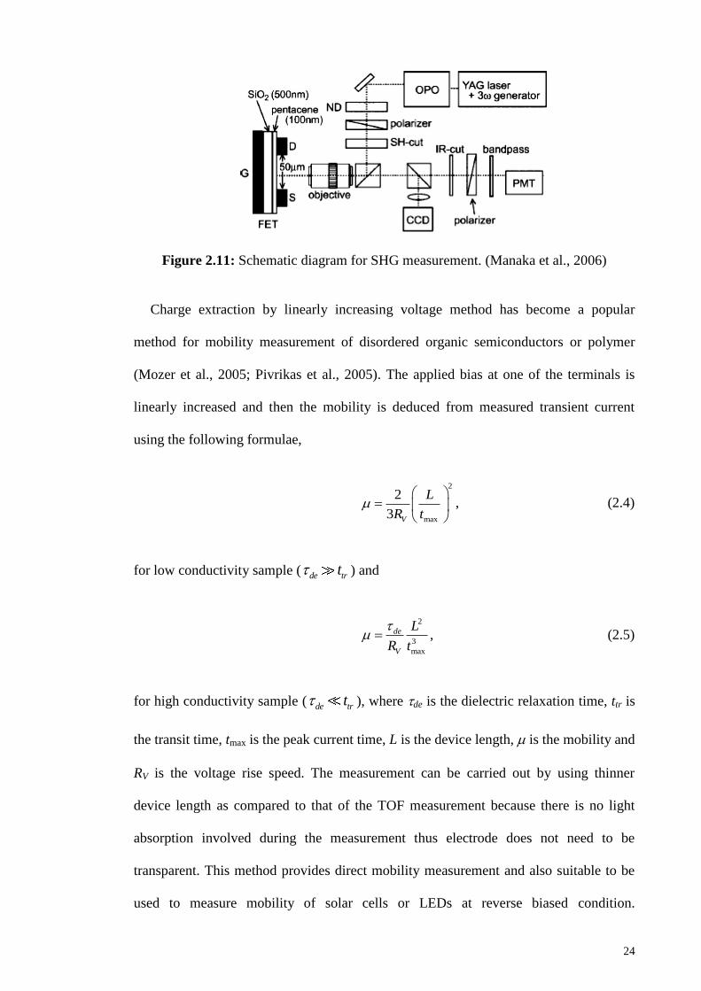
24

Figure 2.11: Schematic diagram for SHG measurement. (Manaka et al., 2006)

Charge extraction by linearly increasing voltage method has become a popular

method for mobility measurement of disordered organic semiconductors or polymer

(Mozer et al., 2005; Pivrikas et al., 2005). The applied bias at one of the terminals is

linearly increased and then the mobility is deduced from measured transient current

using the following formulae,

2

max

2

3 V

L

R t

, (2.4)

for low conductivity sample ( de trt ) and

2

3

max

de

V

L

R t

, (2.5)

for high conductivity sample ( de trt ), where de is the dielectric relaxation time, ttr is

the transit time, tmax is the peak current time, L is the device length, is the mobility and

RV is the voltage rise speed. The measurement can be carried out by using thinner

device length as compared to that of the TOF measurement because there is no light

absorption involved during the measurement thus electrode does not need to be

transparent. This method provides direct mobility measurement and also suitable to be

used to measure mobility of solar cells or LEDs at reverse biased condition.

25

Unfortunately, the mobility for hole and electron of an ambipolar device could not be

distinguished and the charge species with lower mobility will determine the mobility of

the device. This method also requires sufficient amount of charge carriers to be present

in the device for measurable output current. This drawback could be improved by

increasing the amount of charge carriers via doping or light illumination (it is called as

Photo-CELIV (Mozer et al., 2005)). The mobility measurable range depends on the

sample geometry and applied bias range. The extraction time and peak current levels are

proportional to the applied bias ramp speed, which determine the lowest measurable

mobility of the device down to range of 10-5

–10-6

cm2/Vs. In contrast, the upper limit of

the measurable mobility is determined by ratio of the peak current level and RC time

constant. If the ratio is approaching unit, the output current is hard to be distinguished

from the capacitive response.

2.4 Charge transport theories for OFET

Charge transport theory for disordered organic semiconductor or polymer materials

is developed based on the charge transport theory for amorphous semiconductor. This

means that conduction of charge carriers is due to the intermolecular hopping-trapping

process between localised states that are subjected to the energy and positional disorders

of the material. The hopping of a charge carrier from one place to another place in the

device under the influence of an electric field is hypothetically represented by the line in

the Figure 2.12(a). Along the hopping path, the charge carrier has undergone several

hopping through different localised sites with different energy levels as depicted in

Figure 2.12(b). By combining the hopping path in space and energy level, the hopping

of charge transport in two-dimensional energy map is resulted and depicted in Figure

2.12(c). The surface energy is rough due to the material disorder.

26

Figure 2.12: Schematic diagram showing the distribution of transport sites in (a) space,

(b) energy and (c) two dimensional map of energy surface. (Tessler et al., 2009)

The presence of energy disorder is induced by the variation in molecular interaction

energies that results in a broad energy density of states. The positional disorder is

caused by the structural defects such as kinks and twists which are generated in the

polymer chains during fabrication processes. These defects induce variation in the

conjugation lengths and interaction energies. In view of the broad and steep energy

distribution caused by the energy and positional disorder, charge carriers are expected to

be hopping between the localised states that are located near to the transport energy

level or mobility edge. Both exponential and Gaussian distributions are commonly used

in the derivation of the energy DOS in disordered material.

The propagation of charge carrier could be described by a probability evolution

equation, namely master equation, which is given by (Mott & Twose, 1961),

1 1iij i j ji j i ME i i

j

PtTR Pt Pt TR Pt Pt Pt

t

, (2.6)

where j i, Pti(t) is the probability that site i at location Ri and energy Ei is occupied by

a charge carrier or excitation at time t, 1 Ptj(t) is the probability that site j is empty,

TRij is the transition rate from site i to site j and ME-i is the decay rate of the excitation

at site i. The hopping rate from one site to another empty site could be represented

27

either by the Miller-Abrahams transition rate, Mott variable range hopping model,

Marcus transition rate or Gaussian disorder model.

Miller-Abraham transition rate is derived based on the phonon tunnelling mechanism

in semiconductor materials (Miller & Abrahams, 1960). The hopping of charge carriers

is assumed to be near the Fermi level, empty sites are randomly distributed in energy

and no polaron effect. The MATR is given by (Stafström, 2010; Tessler et al., 2009),

2 exp if

exp1 if

ij B j i

ij pho

j ia

R E k T E ETR

E El

, (2.7)

where pho is the phonon vibration frequency or jump-escape rate, la is the localisation

radius, E = Ej – Ei, Ei and Ej are the energy levels at site i and site j.

Mott variable range hopping model is also derived based on the phonon tunnelling

mechanism incorporated with polaron effect for disordered material (Mott & Twose,

1961). The hopping of charge carriers could have happened through resonance and

empty sites are randomly distributed in terms of energy and position. The transition rate

is given by (Dunlap & Kenkre, 1993; Holstein, 1959),

22

exp2 2 2 8

MH

ij p

ij

p B B B B p

E EETR

E k T k T k T k TE

(2.8)

where Ep is the polaron binding energy, Ea = Ep/2 is the polaron activation energy and

MH

ij is the transfer matrix element given by

0

2exp

ijMH MH

ij

a

R

l

, (2.9)

28

and 0

MH is calculated from the crossing point between the reactant (initial state) and

product (final state) energy curves. Equation (2.9) is resulted by assuming that the

electronic coupling between the two energy states decays exponentially with the

distance between the two localised sites.

In the Marcus theory, the initial state, final state and ground state are represented by

identical parabolic energy dispersive curve and shifted relative to each other based on

the Gibbs free energy of the system. Transition of charge carrier occurs through the

minimum energy at the intersecting of the potential surfaces of the initial and final

states. The Marcus transition rate is given by (Likhtenshtein, 2012; Stafström, 2010),

2022

exp44

MC

ij

ij

BB

G ETR

E k TE k T

, (2.10)

where E = 4Ea is the reorganisation energy (energy needed for vertical charge carrier

transfer without the ground state of the charge carrier is being refilled), G is the Gibbs

free energy between the initial and final states, and the MC

ij is the transfer matrix

element given by

0 expijMC MC

ij

a

R

l

, (2.11)

or Equation (2.11) can be rewritten in terms of the polaron activation energy Ea as

202

exp4 16

MCaij

ij

a B a B

G ETR

E k T E k T

. (2.12)

Gaussian disorder model had been proposed by Bässler to model charge transport in

disordered organic photoconductor (Bässler, 1993) and later on this model had been

29

widely used in charge transport study of doped polymers and disordered materials

(Borsenberger et al., 1993; Hartenstein et al., 1995). This model assumes that the

energies of hopping sites for either electron or hole are subjected to a Gaussian

distribution, thus the Gaussian DOS is given by,

2

22

1exp

22 EE

EE

, (2.13)

where energy E is measured relative to the centre of the DOS. The relationship between

the standard deviation E of the Gaussian DOS and the reduced energy disorder

parameter is given by

ˆ EE

Bk T

, (2.14)

and it is related to the dispersive parameter in the time-fractional drift-diffusion

equation (see Equation (3.8)) as ˆ1 . The topological defects that occur in the

polymer chain result in the space localisation of energy states and energies of

neighbouring sites are uncorrelated. The motion of charge carriers is highly random and

the hopping from site i to j is expressed by the MATR as given in Equation (2.7). Monte

Carlo method is then used to simulate the charge carrier transport and the material

disorder is implemented by (i) choosing the reduced energy disorder parameter from the

Gaussian DOS in Equation (2.13), (ii) the distances between the intersites is randomly

chosen from a uniform distribution and (iii) the intersite overlap or coupling parameter

c = 2a/la is taken from a Gaussian distribution, a is lattice constant and c is fixed at 10

as an experiment fitting parameter. The mobility is deduced from the average arrival

time of charge carriers to exceed the device. It should be equal to the transit time of the

plateau region of a non-dispersive current which is obtained from the TOF

30

measurement. The diffusion coefficient is calculated from the variance of the charge

carrier packet or the MSD as

2

2

x xD

t

. (2.15)

Besides the charge transport models presented in the preceding paragraphs, random

walk and central limit theorem used in normal diffusion are respectively generalised to

the continuous-time random walks and generalised central limit theorems for modelling

of charge transport in disordered material (Metzler & Klafter, 2000a; Metzler et al.,

1999; Scher & Montroll, 1975). Several works have attempted to unify both normal and

anomalous transports in a single theoretical framework by means of the generalisation

of normal transport equation using fractional calculus approach. The anomalous

transport models based on fractional calculus have been demonstrated in various forms

such as the fractional diffusion equation (Balakrishnan, 1985; Bisquert, 2005; Hilfer,

2000b; Schneider & Wyss, 1989; Wyss, 1986), fractional Fokker-Planck equation

(Barkai, 2001; Barkai et al., 2000; Metzler et al., 1999), fractional drift-diffusion

equations (Metzler & Klafter, 2004; Sibatov & Uchaikin, 2009), fractional Langevin

equation (Bazzani et al., 2003; Lim & Muniandy, 2002; Lutz, 2001; Metzler & Klafter,

2000b), fractional Brownian motion (Mandelbrot & Van Ness, 1968) and fractional

Klein-Kramer equation (Gajda & Magdziarz, 2011).

Barkai (2001) has developed a FFPE, which is compatible with the CTRW model

that was developed by Scher and Montroll (1975), to describe the anomalous behaviour

of the transient current of amorphous material. Since the probability density of the FFPE

developed by Barkai (2001) is normalised, thus the total charge carriers are conserved

and equivalent to the total charge carriers that are generated during the photo-absorption

process, particularly valid for the case in TOF measurement. Besides, Hilfer had

31

proposed a non-conserved version of the FDE based on the RL fractional derivative to

study anomalous diffusion by replacing the integer order time derivative of the standard

diffusion equation with a fractional order time derivative (Hilfer, 2000b). It was also

suggested that the fractional time derivative with order ranges from 0 to 1 may be

interpreted as infinitesimal generator of time evolution of free charge carriers in

disordered media. Bisquert (2005) had proved that the non-conserved FDE reported in

(Hilfer, 2000b) is capable of providing physical insight of the anomalous diffusion of

free charge carriers in disordered material with dissipation process such as trapping or

recombination mechanism. Sibatov and Uchaikin (2009) has also demonstrated various

versions of conserved TFDDE, incorporated with multiple-trapping mechanism and

recombination of charge carrier, to describe the anomalous diffusion of photo-generated

charge carriers under the influence of external electrical force in amorphous

semiconductors.

2.5 Fractal theory

The term 'fractal' is coined by Benoît Mandelbrot in 1975 based on the Latin word

'frangere' which means broken (Mandelbrot, 1982). A fractal possesses a few

characteristics such as (i) self similarity in which an object or geometric shape could be

infinitely subdivided into small parts and each of them has a similar shape but reduced

size of the original, (ii) scale-invariant which demonstrates the object has fine structure

across different scales, (iii) a fractal dimension Df which can take a non-integer value

and strictly greater than its topological dimension DT. Fractal dimension is considered

as a measure of the space-filling capacity of the fractal object within the environment

where it is contained, and (iv) the relationship between the number of rescaled copies Nf

to cover the original object and the scaling factor rf takes a power law form in which the

fractal dimension Df is being the scaling exponent.

32

One of the methods used to obtain the fractal dimension of an object is called Box

counting method. A square box with size WB is used to cover the fractal object and the

number of box NB with size WB is needed to cover the whole object of area A is

recorded. The relationship between NB and WB is given by

1

BB D

B

NW

, (2.16)

where DB is the box dimension (Minkowski-Bouligand dimension). The measurement

process is repeated with different box sizes. The box dimension is then obtained from

the slope of the linear least square line that passing through all the points in the log(NB)

versus log(1/WB) plot. The box dimension is also defined as

0

loglim

log 1B

BB

WB

ND

W . (2.17)

Similarly, the Hausdorff dimension DH can be obtained using the similar procedures as

that of the box counting method but the fractal object is covered with varying box sizes.

Besides, PSD method (see subsection 3.3.1) and DFA (see subsection 3.3.2) could also

be used to estimate the scaling exponent and fractal dimension of fractal objects.

Fractal object can be classified, based on its similarity property, as (i) exact self-

similarity, (ii) quasi-self-similar and (iii) self-affinity. Exact self-similarity is defined as

the set which has the same pattern at all scales. The Sierpinski triangle and von Koch

curve are the examples of exact self-similarity geometry as depicted in Figure 2.13 and

Figure 2.14, respectively. A Sierpinski triangle could be generated by first taking the

midpoints of each side of a triangle (represented by the black triangle in stage 0 as

shown in Figure 2.13) to form the vertices of a new triangle (represented by the white

triangle in stage 1) which is then removed from the original triangle. Three black similar

33

shape triangles are formed in the original triangle but each of them has only one-fourth

the original area and half the original dimension. The same procedure is repeated at

each of the black triangle in stage 1, thus nine smaller black triangles are resulted in

stage 2. Each of them has only one-fourth the original area and half the original

dimension of the triangle in stage 1. After n iteration, the number of triangles produced

is 3n

fN , the dimension is 1 2n and the area is 1 4

n. The fractal dimension of the

Sierpinski triangle is calculated as log3 log 1/ 2 1.585fD .

Figure 2.13: Sierpinski triangle. (Fractal organisation)

Von Koch curve, which was developed by Niels Fabian Helge von Koch, can be

formed by first removing and replacing the 1/3 middle part of a linear line (initiator, E0)

with the two other sides of an equilateral triangle to arrive at stage E1, as shown in

Figure 2.14. After that, this rule is generated for infinite subsequent levels to ultimately

form the von Koch curve (Falconer, 1990). The length of the von Koch curve becomes

infinite due to an additional 1/3 length is added onto the curve at every stage. The

fractal dimension of the von Koch curve can be calculated as, log4 log3 1.26fD .

Besides, three von Koch curves can be connected together to form a von Koch

snowflake.

34

Figure 2.14: (a) von Koch curve at different level of magnification and (b) von Koch

snowflake. (Falconer, 1990)

Quasi self-similarity is defined as the set which has arbitrarily small parts of the set

that can be magnified and altered smoothly to coincide with a large part of the set.

Examples of quasi self-similarity objects are the star-like branching structure of

polystyrene and Julia set as shown in Figure 2.15 and Figure 2.16, respectively. As

shown in Figure 2.15, the structure of a group of polymer branches takes on a star-

shaped structure and the structure of a smaller branch partially bears a resemblance to

the whole structure. Star-shaped macro-initiators are first synthesised from the

polystyrene initiators using the convergence technique and the star-shaped macro-

initiators will then be converged to form the radially linked star-block-linear

Polystyrene polymer as showed in Figure 2.15 (Knauss & Huang, 2003).

35

Figure 2.15: Radially linked star-block-linear polystyrene polymers. (Knauss & Huang,

2003)

Julia set, named after Gaston Maurice Julia, which can be described by a quadratic

function, 2f z z c , for a constant c and z is the position in space. For a constant

value of c = 1, the Julia set has a fractal dimension of 1.27 and the pattern is depicted

in Figure 2.16 (McMullen, 1998).

Figure 2.16: Julia set. (McMullen, 1998)

Self-affinity is defined as the set which has pattern possesses same statistical

properties at all scales. Romanesco broccoli, fern leaf, morphology of Physarum

Polycephalum plasmodium, coastline of Britain and Mandelbrot set are some examples

36

of self-affinity sets. Figure 2.17 shows a Romanesco broccoli and its florets which are

disengaged from the original structure at various scales but yet they still resemble the

whole structure of the broccoli and demonstrate the present of self-similar property. The

arrangements of florets follow certain spiral path where the path begins from the top

centre of the broccoli. The spiral path is defined by the Fibonacci spiral (a series of arcs

whose radius values are given by the Fibonacci sequence) and the number of spiral

paths in a direction is defined by the successive Fibonacci numbers. Besides, the

Fibonacci number could also be used to model other fractal nature objects such as the

number of branches of tree, arrangement of leafs around tree stem or stump, pattern on

the shell of Chambered nautilus and ratio between human fingers and forearm.

Figure 2.17: Romanesco broccoli at different magnification levels. (King, 2016)

Figure 2.18 shows a spleenwort fern which is decomposed into four magnification

levels and all the rescaled copies (branches) of the fern look alike the whole structure of

the fern. This shows that fern is one of the natural fractal sets that possesses self-

similarity property.

37

Figure 2.18: Fern leaf decomposed to four magnification levels.

Michael Barnsley, a British mathematician, had developed the mathematical

formulation and computer algorithm based on the iterated function system, to replicate

the pattern of fern (Barnsley, 1993). In the IFS method, the procedures to generate the

fern are (i) generating a starting point randomly, (ii) choosing one out of the four sets of

coordinate transformations based on its assigned probability, (iii) multiplying the

chosen starting point in step (i) by the transformation matrix and then sum with the

translation matrix, (iv) the resulting point is then fed as the starting point to generate the

next new point and (v) repeating steps (ii) to (iv) for many iterations. Since the whole

Barnsley Fern, named after Michael Barnsley, generation process is based on the

randomly chosen numbers, thus the Barnsley Fern is considered as a chaotic IFS fractal

sets. The computer generated Barnsley Fern is shown in Figure 2.19 and its fractal

dimension is estimated to be around 1.45.

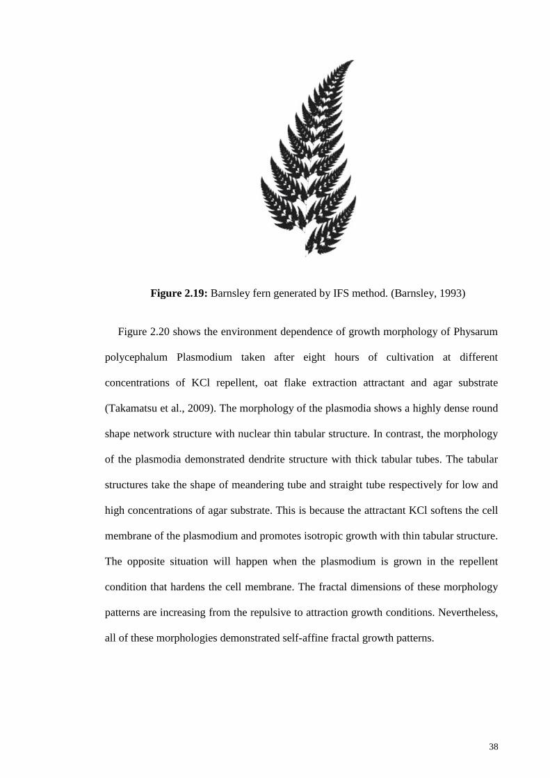
38

Figure 2.19: Barnsley fern generated by IFS method. (Barnsley, 1993)

Figure 2.20 shows the environment dependence of growth morphology of Physarum

polycephalum Plasmodium taken after eight hours of cultivation at different

concentrations of KCl repellent, oat flake extraction attractant and agar substrate

(Takamatsu et al., 2009). The morphology of the plasmodia shows a highly dense round

shape network structure with nuclear thin tabular structure. In contrast, the morphology

of the plasmodia demonstrated dendrite structure with thick tabular tubes. The tabular

structures take the shape of meandering tube and straight tube respectively for low and

high concentrations of agar substrate. This is because the attractant KCl softens the cell

membrane of the plasmodium and promotes isotropic growth with thin tabular structure.

The opposite situation will happen when the plasmodium is grown in the repellent

condition that hardens the cell membrane. The fractal dimensions of these morphology

patterns are increasing from the repulsive to attraction growth conditions. Nevertheless,

all of these morphologies demonstrated self-affine fractal growth patterns.

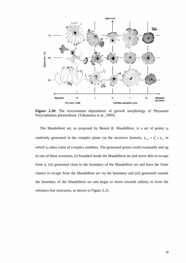
39

Figure 2.20: The environment dependence of growth morphology of Physarum

Polycephalum plasmodium. (Takamatsu et al., 2009)

The Mandelbrot set, as proposed by Benoit B. Mandelbrot, is a set of points z0

randomly generated in the complex plane via the recursive formula, 2

1 0n nz z z , in

which z0 takes value of complex numbers. The generated points could eventually end up

in one of these scenarios, (i) bounded inside the Mandelbrot set and never able to escape

from it, (ii) generated close to the boundary of the Mandelbrot set and have the finite

chance to escape from the Mandelbrot set via the boundary and (iii) generated outside

the boundary of the Mandelbrot set and begin to move towards infinity to form the

whiskers line structures, as shown in Figure 2.21.

40

Figure 2.21: Mandelbrot set. (Falconer, 1990)

As shown in Figure 2.22, the coastline of the Great Britain demonstrated high

irregularity and winding characteristics in which its total length of coastline varies with

the method employed to measure it. The length of the coastline can be measured by first

defining the window length WL of a measuring device and then moving the window

along the coastline by sequentially placing the new window on the end point of the

previous step. Thus, the total length of the coastline L(WL) is simply calculated as

L L LL W N W , (2.18)

and it is related to the fractal dimension through

f

LL D

L

WL W

W , (2.19)

where NL is the number of steps covering whole coastline which is given by

1

fL D

L

NW

, (2.20)

41

and Df is the fractal dimension (Mandelbrot, 1982). As the measurement is repeated

with gradually decreasing window length, the actual length of the coastline is expected

to be obtained since the coastline is better mapped at very fine scale. However, the

measurement shows that the measured length L(WL) is likely to increase infinitely. This

imposes a difficulty to determine the actual length of the coastline as its length varies

with the window length used in the measurement. This phenomenon was named as

Richardson effect in 1961 after Lewis Fry Richardson. The fractal dimension calculated

for the coastline of Britain is Df = 1.25.

Figure 2.22: Coastline of Great Britain. (“Geometric Fractal - Chapter 2 Fractal

Dimension of Coastlines”)

The idea of self-similarity is also extended to mathematical function namely the

Weierstrass function, proposed by Karl Weierstrass in 1875, which is a continuous

function but not differentiable at any point on the function. The Weierstrass function is

given by, (Mandelbrot, 1982),

2

0

1exp 2

1

k k

W

k

f t w ib tw

, (2.21)

where real number b 1, w = bH, the Hölder exponent H has the range of 0 H 1 and

the fractal dimension Df = 2 H for 1 Df 2. The Weierstrass function fW(t) generated

for various H values (H = 0.1, 0.3, 0.5 and 0.7) are depicted in Figure 2.23. It can be

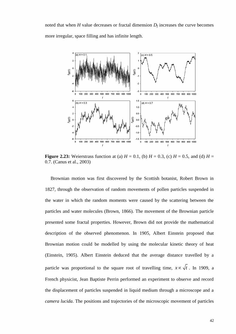
42

noted that when H value decreases or fractal dimension Df increases the curve becomes

more irregular, space filling and has infinite length.

Figure 2.23: Weierstrass function at (a) H = 0.1, (b) H = 0.3, (c) H = 0.5, and (d) H =

0.7. (Canus et al., 2003)

Brownian motion was first discovered by the Scottish botanist, Robert Brown in

1827, through the observation of random movements of pollen particles suspended in

the water in which the random moments were caused by the scattering between the

particles and water molecules (Brown, 1866). The movement of the Brownian particle

presented some fractal properties. However, Brown did not provide the mathematical

description of the observed phenomenon. In 1905, Albert Einstein proposed that

Brownian motion could be modelled by using the molecular kinetic theory of heat

(Einstein, 1905). Albert Einstein deduced that the average distance travelled by a

particle was proportional to the square root of travelling time, x t . In 1909, a

French physicist, Jean Baptiste Perrin performed an experiment to observe and record

the displacement of particles suspended in liquid medium through a microscope and a

camera lucida. The positions and trajectories of the microscopic movement of particles

43

were recorded at regular time intervals and respectively represented by the dots and

lines as shown in Figure 2.24. The recorded trajectories demonstrated the stochastic

nature of the movements of particles due to the collisions with water molecules. Perrin

concluded that the mean squared distance travelled by particles changes linearly with

time and reaffirmed the molecular kinetic theory of heat developed by Albert Einstein

(Bigg, 2008; Perrin et al., 1910). He also pointed out that the irregular movements of the

particles coincided with non-differentiable continuous functions.

Figure 2.24: Displacement of three particles recorded in the experiment conducted by

Perrin. (Perrin et al., 1910)

Almost two decades later, an American Mathematician, Norbert Wiener, had

rigorously developed the mathematical framework to describe the trajectory followed by

a single particle or Brownian motion based on the continuous non-differentiable

function theory (Wiener, 1923). Brownian motion is a random process B(t) which has

the following properties (Mandelbrot, 1982):

(i) With probability of 1, B(0) = 0, B(t) is continuous, Gaussian distributed and

nonstationary.

(ii) B(t) possesses self-affinity which gives 0.5 , 0B t s B st s and it will be

regenerating itself at every time instant which leads to short memory effect.

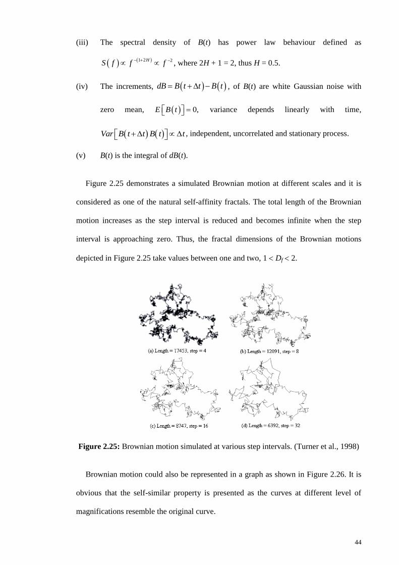
44

(iii) The spectral density of B(t) has power law behaviour defined as

1 2 2HS f f f

, where 2H + 1 = 2, thus H = 0.5.

(iv) The increments, dB B t t B t , of B(t) are white Gaussian noise with

zero mean, 0,E B t variance depends linearly with time,

Var B t t B t t , independent, uncorrelated and stationary process.

(v) B(t) is the integral of dB(t).

Figure 2.25 demonstrates a simulated Brownian motion at different scales and it is

considered as one of the natural self-affinity fractals. The total length of the Brownian

motion increases as the step interval is reduced and becomes infinite when the step

interval is approaching zero. Thus, the fractal dimensions of the Brownian motions

depicted in Figure 2.25 take values between one and two, 1 Df 2.

Figure 2.25: Brownian motion simulated at various step intervals. (Turner et al., 1998)

Brownian motion could also be represented in a graph as shown in Figure 2.26. It is

obvious that the self-similar property is presented as the curves at different level of

magnifications resemble the original curve.

45

Figure 2.26: Brownian function, H = 0.5, at various magnification levels. (Canus et al.,

2003)

Besides, fractal set is sometimes classified as monofractal or multifractal.

Monofractal is the fractal set which possesses only one fractal dimension. For example,

Koch snowflake, Cantor set, coastline of Britain, Brownian motion and fractional

Brownian motion. Multifractal is fractal set which possesses a series of fractal

dimensions, for instances, multifractal Brownian motion.

2.5.1 Fractal modelling of signals and surfaces

Fractional Brownian motion is another example of a mathematical function that

presents self-affinity pattern as depicted in Figure 2.27. The reduction in H value

decreases the jaggedness and also smoothens the curve. Brownian motion with H = 0.5

is a special case of the FBM.

46

Figure 2.27: Fractional Brownian motion at various H values. (Canus et al., 2003)

Fractional Brownian motion is derived by Benoit B. Mandelbrot using the RL

fractional integral as (Mandelbrot, 1982; Mandelbrot & Van Ness, 1968):

1/2

0

1

1/ 2

t Ht s dB s

H

, (2.22)

where dB(u) is the white noise. Equation (2.22) will exit if s t, H should be positive

value and achieve stationary increments, thus Equation (2.22) is rewritten using the

Weyl’s integral as,

1/21

1/ 2

t H

BB t t s dB sH

. (2.23)

Since t could attain values from both the directions of the coordinate, thus it will be

more practical to write the Equation (2.23) in its symmetric form which is defined as,

0 1/2 1/2 1/2

0

1.

1/ 2

tH H H

HB t t s s dB s t s dB sH

(2.24)

47

Equation (2.24) is called the FBM and its properties are given below:

(i) With probability of 1, BH(0) = 0, BH(t) is continuous, random, Gaussian

distributed and nonstationary process.

(ii) BH(t) possesses self-affinity which gives , 0H

H HB t s B st s and it will be

regenerating itself at every time instant which leads to short memory effect.

(iii) The spectral density of BH(t) has power law behaviour defined as

1 2PS

HS f f f

, where PS = 2H + 1 is the power spectra scaling

exponent. White noise, 1/f noise and Brownian noise are respectively

represented by PS = 0, PS = 1 and PS = 2.

(iv) The increments, H H HdB B t t B t , of the FBM BH(t) are called the

fractional Gaussian noise with zero mean, 0HE B t , covariance depends

linearly with time, 2H

H HVar B t t B t t , independent, uncorrelated

and stationary process.

(v) BH(t) is the integral of dBH(t).

(vi) The fractal dimension of the FBM is given by 2fD H .

Since the power spectra scaling exponents PS could be used to characterise the

fractal or scaling behaviour of a time series (either a signal or noise), thus the PSD

method and FBM could be used for time series analysis or modelling. Nevertheless,

FBM could also be used for surface and terrain analysis and modelling. Figure 2.28

shows typical examples of fractal surfaces which are generated using the fractional

Brownian motion in two dimensional spaces for different values of H ranging from 0.1

to 0.7. At small H value, the surface forms many small clusters and spread randomly

throughout the whole area. Oppositely, the surface forms few large clusters and contain

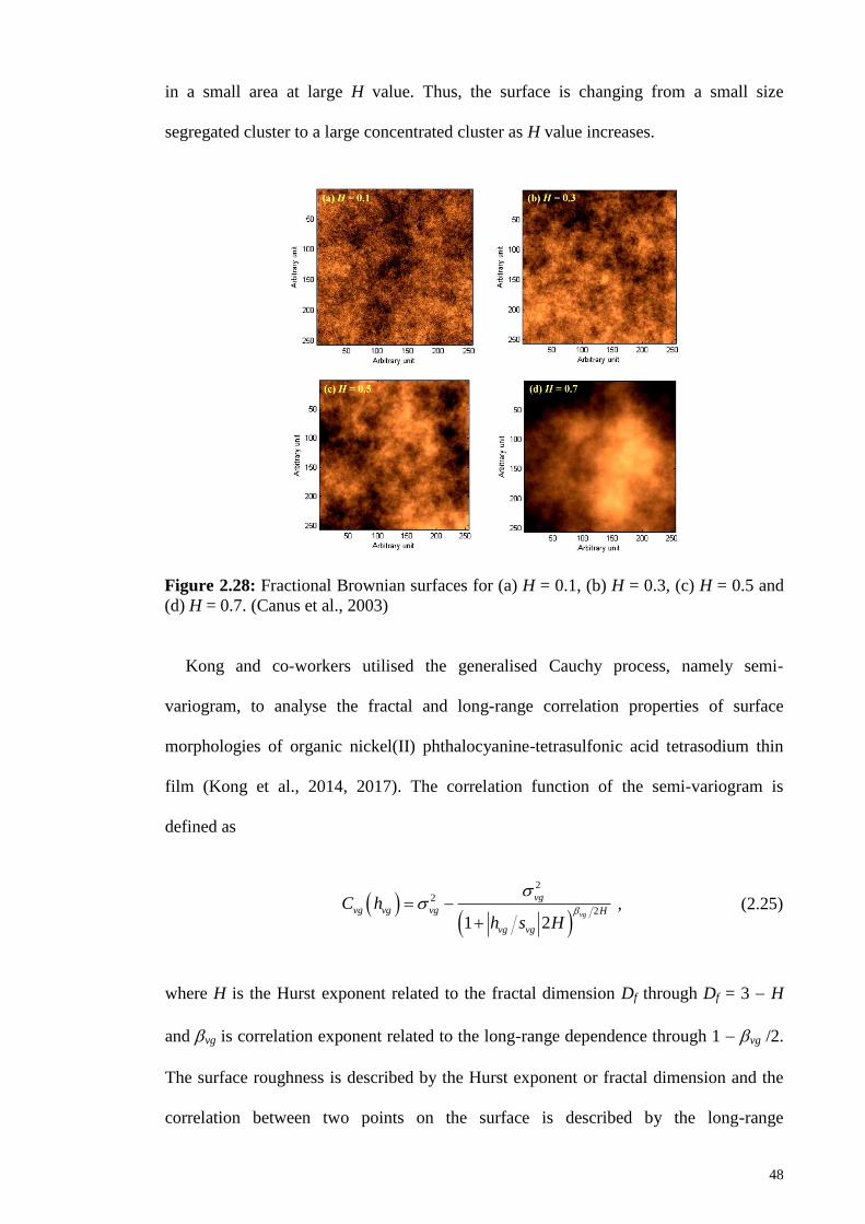
48

in a small area at large H value. Thus, the surface is changing from a small size

segregated cluster to a large concentrated cluster as H value increases.

Figure 2.28: Fractional Brownian surfaces for (a) H = 0.1, (b) H = 0.3, (c) H = 0.5 and

(d) H = 0.7. (Canus et al., 2003)

Kong and co-workers utilised the generalised Cauchy process, namely semi-

variogram, to analyse the fractal and long-range correlation properties of surface

morphologies of organic nickel(II) phthalocyanine-tetrasulfonic acid tetrasodium thin

film (Kong et al., 2014, 2017). The correlation function of the semi-variogram is

defined as

2

2

2

1 2vg

vg

vg vg vg H

vg vg

C hh s H

, (2.25)

where H is the Hurst exponent related to the fractal dimension Df through Df = 3 H

and vg is correlation exponent related to the long-range dependence through 1 vg /2.

The surface roughness is described by the Hurst exponent or fractal dimension and the

correlation between two points on the surface is described by the long-range

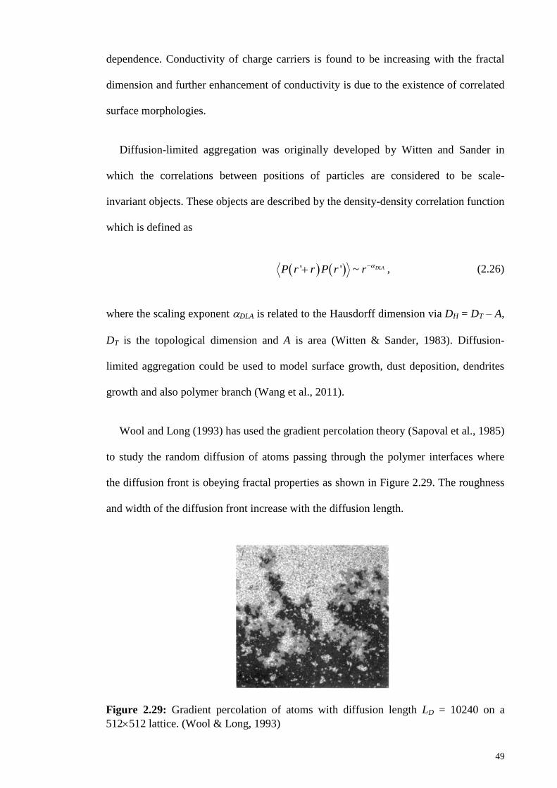
49

dependence. Conductivity of charge carriers is found to be increasing with the fractal

dimension and further enhancement of conductivity is due to the existence of correlated

surface morphologies.

Diffusion-limited aggregation was originally developed by Witten and Sander in

which the correlations between positions of particles are considered to be scale-

invariant objects. These objects are described by the density-density correlation function

which is defined as

' ' ~ DLAP r r P r r

, (2.26)

where the scaling exponent DLA is related to the Hausdorff dimension via DH = DT – A,

DT is the topological dimension and A is area (Witten & Sander, 1983). Diffusion-

limited aggregation could be used to model surface growth, dust deposition, dendrites

growth and also polymer branch (Wang et al., 2011).

Wool and Long (1993) has used the gradient percolation theory (Sapoval et al., 1985)

to study the random diffusion of atoms passing through the polymer interfaces where

the diffusion front is obeying fractal properties as shown in Figure 2.29. The roughness

and width of the diffusion front increase with the diffusion length.

Figure 2.29: Gradient percolation of atoms with diffusion length LD = 10240 on a

512512 lattice. (Wool & Long, 1993)

50

The diffusion front is characterised by the mass-to-radius relation as

fD

D Dm r , (2.27)

where mD is the mass, rD is the radius and Df is the fractal dimension. The width of the

diffusion front f is related to the diffusion length LD as

f

f DL

, (2.28)

and the scaling exponent of DLA (f) is related to the percolation exponent and

fractal dimension as

11

f fD

. (2.29)

2.5.2 Fractal dynamics

Stanley formerly published a work describing how fractal concepts could be applied

to polymer and anomalous transport in porous media (Stanley, 1984). An example is the

relation between the fractal dimension of backbone of polymer with electric current

flow and random walker. In crystalline media, the Fick’s diffusion law defines that the

r.m.s. displacement x2

0.5 of a random walker is linearly proportional to the number of

steps NW made by the walker which is given by

0.5

2

Wx N . (2.30)

If a random walker is moving in a porous media, it will only be able to travel a smaller

distance away from its origin as compared to the random walker that is moving in a

crystalline material. Thus, Equation (2.30) is redefined as

51

0.5

2 WD

Wx N , (2.31)

where DW 1 (Stanley, 1984). Equation (2.31) is equivalent to the mass-to-radius

relation given by Equation (2.27). Let’s say that the random walk represents the free

flight polymer chain and the walker represents the charge carrier propagating along the

backbone of the chain which is characterised by the fractal dimension, thus 1/DW is

equivalent to the fractal dimension Df of the random walker (polymer chain), number of

walker steps NW is equivalent to the mass of the polymer chain mD and r.m.s.

displacement is equivalent to the length of the random walk. Since the electrical current

density is proportional to the velocity of charge carriers, thus electrical current density

could be calculated by taking the time rate of change of MSD of the random walkers

multiplied by the electronic charge and density of charge carriers.

Diffusion is a Markov process which could be considered as a continuous time

stochastic process with continuous paths if the changes in time and space are infinitely

small. Thus, diffusion process could be represented by Brownian motion or Wiener

process through a stochastic differential equation that takes the form of (Øksendal,

2003),

, ,t t t tdX t X t X dW , (2.32)

where dWt is white noise (time derivative of Wiener process or Brownian motion),

(t,Xt) is a drift coefficient and (t,Xt) is a diffusion coefficient. White noise is a

stochastic process with Gaussian distribution and zero mean. Since Wt is a continuous

but non-differential function, Equation (2.32) could not be solved directly and usually is

written in its integral form as

0

0 0

, ,t t

t t s s st t

X X s X ds s X dW , (2.33)

52

and the solution Xt of Equation (2.33) gives the diffusion process.

2.6 Normal diffusion theory for charge transport in ordered material

This subsection provides the introduction to several charge transport theories which

are formulated for normal diffusion process adopted in crystalline media. These

transport models could be generalised using the fractional calculus to model the

anomalous diffusion in disordered material. Thus, the concept of fractional calculus is

given before the description of the anomalous transport theories.

(a) Diffusion equation based on Fick's law and law of conservation of mass

In 1885, Adolf Fick published his work entitled "Uber Diffusion" in Annalen der

Physik which described diffusion of particles in liquid medium confined by membranes

is due to the existence of concentration gradient. The existence of concentration

gradient causes particles to begin moving away from the high concentration region to

their surrounding regions with lower concentration till the equilibrium of concentration

is achieved.

According to Fick’s first law (Fick, 1855), the flow current density of particles is

proportional to the concentration gradient which is written as

,

,c x t

j x t Dx

, (2.34)

where D is the diffusion coefficient with dimension of L2/T, c(x,t) is the concentration of

particle, x is the position in one-dimensional Cartesian-coordinate space and t is time of

particle at x. Based on the law of conservation of mass, the continuity equation is

defined as

, ,c x t j x t

t x

. (2.35)

53

By substituting Equation (2.34) in Equation (2.35), Fick’s second law, which is also

commonly known as the diffusion equation, is resulted as

2

2

, ,c x t c x tD

t x

. (2.36)

The diffusion equation in Equation (2.36) describes the temporal evolution of the

concentration.

(b) Drift-diffusion equation based on Fick's law

If the particle is subjected to an external force F(x), the continuity equation is

rewritten as

,

, ,c x t

j x t x c x t Dx

, (2.37)

where v(x) = F(x) is the velocity of the particle and is the mobility. Thus, the drift-

diffusion equation is resulted when Equation (2.37) is substituted into Equation (2.35)

and it is written as

2

2

, ,,

c x t c x tD F x c x t

t x x

. (2.38)

(c) Diffusion equation based on random walk theory

In 1905, Albert Einstein (1905) derived the diffusion equation for random walker (or

Brownian molecular motion) based on the postulates of molecular kinetic theory of heat

in which particles move independently subjected to the influence of thermal energy.

Let’s say a particle is located at the origin and it has an equal probability of jumping an

equal length x to the left or to the right empty site at each short time interval t. The

54

state probability P(x,t) of the particle will be at position x = ix and at time t = kt is

given by

1 1

, , ,2 2

P x t P x x t t P x x t t . (2.39)

By expanding the two probability terms, in the R.H.S. of Equation (2.39), using the

Taylor-series expansion, one gets

2 22 2

2 2

23 3

, ,, ,

, ,

2 2

,,

P x t P x tP x x t t P x t x t

x t

x P x t t P x t

x t

P x tx t O x O t

x t

(2.40)

and

2 22 2

2 2

23 3

, ,, ,

, ,

2 2

,.

P x t P x tP x x t t P x t x t

x t

x P x t t P x t

x t

P x tx t O x O t

x t

(2.41)

Retain only the leading order terms in x and t, and then substitute Equation (2.40)

and Equation (2.41) into Equation (2.39), thus one gets the diffusion equation for one-

dimensional space as

2,

,P x t

D P x tt

, (2.42)

55

where 2

2D x t is the diffusion coefficient and the probability P(x,t) of finding

the particle at x and time t is related to the concentration of particle c(x,t) which is given

by

, ,c x t NP x t , (2.43)

and N is the total number of particles in the system. By solving Equation (2.42), the

propagation of particle away from the origin of coordinates in one-dimensional space is

given by

2 4

1 2

1,

4

x DtP x t eDt

. (2.44)

The mean squared displacement of the particle is then given by

2 2 3, 2x t x P x t d x Dt

. (2.45)

Thus, Equation (2.45) demonstrated that the MSD of the normal diffusion of random

walker is linearly proportional to time or 2x t t .

(d) Advection-diffusion equation based on random walk theory

If a particle is located at the origin and subjected to an external force, the probability

of the particle to jump a length x to the left empty site is not the same as the

probability of the particle to jump the same length to the right empty site at each short

time interval t. Let’s define that r1 and r2 are the transition probability of flow to right

and left, respectively. The state probability P(x,t) of the particle will be at position x =

ix and at time t = kt is given by

2 1, , ,P x t r P x x t t r P x x t t . (2.46)

56

By expanding the two probability terms, in the R.H.S. of Equation (2.46), using the

Taylor-series expansion, one gets

1 1 1 1

2 22 2

1 1

2 2

23 3

1

, ,, ,

, ,

2 2

,,

P x t P x tr P x x t t r P x t r x r t

x t

r x P x t r t P x t

x t

P x tr x t O x O t

x t

(2.47)

and

2 2 2 2

2 22 2

2 2

2 2

23 3

2

, ,, ,

, ,

2 2

,.

P x t P x tr P x x t t r P x t r x r t

x t

r x P x t r t P x t

x t

P x tr x t O x O t

x t

(2.48)

Retain only the leading order terms in x and t, and then substitute Equation (2.47)

and Equation (2.48) into Equation (2.46), thus one gets the advection-diffusion equation

for one-dimensional space as

2

2

, , ,P x t P x t P x tD

t x x

, (2.49)

where 2

2D x t is the diffusion coefficient and 1 2r r x t is advection

coefficient. The second term on the R.H.S. of Equation (2.49) represents the advection

flow of particles due to the external force. Equation (2.49) is considered as the

Smoluchowski equation (Smoluchowski, 2010) and similar to drift-diffusion equation

(see Equation (2.38)) when the probability P(x,t) is replaced by the concentration of the

charge particle as given by Equation (2.43). The resulted partial differential equation

57

represents the time evolution of the concentration profile of particles simultaneously

due to diffusion and advection processes.

Let’s say the external force is given by F(x) = dV(x)/dx, which is induced by an

applied potential V(x), Equation (2.49) can be rewritten as, (Coffey et al., 2004; Fokker,

1914; Risken & Frank, 1996),

2

2

, ,,

LE

P x t P x t F xD P x t

t x x m

, (2.50)

where m is the mass of particle, LE is the friction constant and the diffusion coefficient

D can be given by the Einstein-Stokes-Smoluchowski relation as D = kBT/mLE

(Einstein, 1905; Hughes, 1995; Kubo, 1966). Equation (2.50) is a specialised form of

the Fokker-Planck equation which is known as the Smoluchowski equation (Mazo,

2009).

(e) Diffusion equation based on Langevin equation

When a particle is suspended in a liquid and subjected to an external force, it will

experience frictional drag acting against its motion and random collisions with the

thermal agitated liquid molecules as it is moving from one place to another place. The

motion of the particle can be described by a stochastic differential equation for

Brownian motion, namely Langevin equation, given by (Kubo, 1966; Zwanzig, 2001),

2

2 LE LE

d xm F x m t

dt , (2.51)

where m is the mass of the particle, is the viscosity of the fluid, LE LE m is the

friction constant, 6LE a LEr is the friction coefficient, ra is the radius of the particle,

is the velocity, F(x) is the external force and mLE is the frictional force. The random

58

fluctuating force due to the collisions of particle with liquid molecules LE(t) is

Gaussian distributed and has the following properties as,

0LE t , (2.52)

and

' 2 'LE LE B LEt t k T t t . (2.53)

Equation (2.53) relates the strength of the fluctuating force to the magnitude of the

friction or dissipation of the liquid which is characterised by LE . This relation is known

as the fluctuation-dissipation theorem (Agarwal, 1972; Kubo, 1966; Zwanzig, 2001).

Besides, the friction coefficient is also related to the diffusion of the particle via the

Einstein-Stokes-Smoluchowski relation as D = kBT/LE. Thus, the frictional coefficient

is also referred as inverse mobility.

2.7 Fractional calculus theory

Fractional calculus has been developed since 1695, almost as old as the integer

calculus, when Gottfried von Leibnitz replied to Guillaume de l'Hôpital after he had

been asked for the meaning of dny/dx

n if n = 1/2 and wrote, "Thus, it follows that d

1/2x

will be equal to :x dx x ,...from which one day useful consequences will be drawn."

(Sokolov et al., 2002). Unlike integer order differential equation which has been widely

accepted and used in describing many physical phenomena, but fractional differential

equation has received very little attention till few decades ago. The foundation of

fractional calculus has been contributed by many great scientist (such as Pierre-Simon

Laplace, Bernhard Riemann, Joseph Liouville, Michele Caputo and many more) before

it could be readily used in describing physical phenomena. The applications of

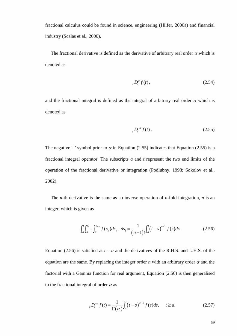
59

fractional calculus could be found in science, engineering (Hilfer, 2000a) and financial

industry (Scalas et al., 2000).

The fractional derivative is defined as the derivative of arbitrary real order which is

denoted as

( )a tD f t, (2.54)

and the fractional integral is defined as the integral of arbitrary real order which is

denoted as

( )a tD f t. (2.55)

The negative '' symbol prior to in Equation (2.55) indicates that Equation (2.55) is a

fractional integral operator. The subscripts a and t represent the two end limits of the

operation of the fractional derivative or integration (Podlubny, 1998; Sokolov et al.,

2002).

The n-th derivative is the same as an inverse operation of n-fold integration, n is an

integer, which is given as

1 1 1

1

1... ( ) ... ( )

1 !

nt s s t n

n na a a a

f s ds ds t s f s dsn

. (2.56)

Equation (2.56) is satisfied at t = a and the derivatives of the R.H.S. and L.H.S. of the

equation are the same. By replacing the integer order n with an arbitrary order and the

factorial with a Gamma function for real argument, Equation (2.56) is then generalised

to the fractional integral of order as

11

( ) ( ) , .t

a ta

D f t t s f s ds t a

(2.57)

60

Thus, fractional derivative of order is defined via the fractional integration and

successive integer differentiation which is mathematically written as

( ) ( )

nn

a t a tn

dD f t D f t

dt

. (2.58)

or

11

( ) ( )n

t n

a t n a

dD f t t s f s ds

n dt

. (2.59)

The number of differentiations is n = [] + 1 where [] is the whole part of . Base on

this definition, the lower limit becomes zero. Equation (2.57) is rewritten as

1

00

1( ) ( )

tRL

tD f t t s f s ds

, (2.60)

where n 1 n Z+

and called the RL fractional integral of order . Similarly,

Equation (2.58) or Equation (2.59) is called the RL fractional derivative of order and

written as

1

00

1( ) ( )

nt nRL

t n

dD f t t s f s ds

n dt

, (2.61)

where n 1 n Z+

. The RL fractional derivative could be viewed as an integral-

differentiation equation.

It should be noted that the RL fractional derivative of a constant is not zero but given

as

0

11

1

RL

tD t

, (2.62)

61

because (1 ) diverges if the fractional derivative order takes a non integer value.

Besides, the Laplace transform of the RL fractional integral results in a simple form as

0

RL

tL D f t u L f t . (2.63)

If the lower limit of Equation (2.57) becomes , the Weyl fractional derivative of

an exponential function yields

W t t

tD e e

. (2.64)

The Fourier transform of the Weyl fractional derivative or integration produces the

similar properties of Fourier transform of integer order derivative or integration,

respectively. For instance,

2

( )W

tF D f t i f . (2.65)

Caputo fractional derivative is a differentiation-integral equation which is given by,

1 ( )

00

1( ) ( )

t nC n

tD f t t s f s dsn

, (2.66)

where n 1 n Z+. Unlike the RL fractional derivative, the Caputo fractional

derivative of a constant is zero.

2.8 Theories of anomalous charge transport

It has been demonstrated that there are many transport processes in physical systems

deviate from the normal diffusion process as their MSD values depend non-linearly on

time. One typical example is the present of long tail transient photocurrent curves of

disordered organic semiconductor measured by the TOF measurement. The following

section will describe how the TOF measurement can be used as an important technique

62

to study the anomalous transport of charge carriers in disordered organic semiconductor.

The related charge transport theories for anomalous diffusion are then described in the

subsequent sub-sections.

2.8.1 Time-of-flight measurement

Time-of-flight measurement is one of the important techniques which can be used to

study the mobility of charge carriers, probing on the information about the defects

located within the surface, interface or bulk material. A basic setup of a TOF

measurement is depicted in Figure 2.30.

Figure 2.30: A basic setup for a TOF measurement. (Scher & Montroll, 1975)

A light pulse, which is generated by a laser source, is shone on a DUT (or TOF cell)

while it is biased. The time taken by a packet of charge carriers to drift across the DUT

is measured and then used to determine the charge carrier transit time ttr. The measured

transient current is given by

0

1,

L

I t j x t dxL

, (2.67)

where j(x,t) is the conduction current density and L is the length or thickness of the TOF

cell.

63

The measured transient current is affected by a few factors such as (i) RC time

constant rc, (ii) loss of charge carriers due to deep energy level trapping, (iii) spatial

variation of mobility due to material inhomogeneity of the DUT, (iv) spatial variation in

electric field due to trapped charge carriers in small signal case, (v) spatial variation in

electric field due to space charge effect in large signal case and (vi) spreading of the

pulse width of charge carrier packet which is comparable to the length of the DUT.

Factors (i) and (ii) impose the practical limit of the TOF measurement and the

condition, RC time constant rc transit time ttr deep trapping lifetime D, must be

embraced in order to obtain a reliable and accurate transient current measurement.

Factors (iii) to (v) induce spatial variation on the drift velocity which ultimately yields

fluctuation in current level that could lead to current noise. Nevertheless, the variation

in drift velocity does not necessarily smear out the step-like current level at the transit

time. Factor (vi) could be connected to various random processes, such as multiple-

trapping, hoping and dispersion of charge carriers due to material inhomogeneity, which

could result in the broadening of pulse width of charge carrier packet, reduction in

current level and smearing of the step-like transit edge as shown in Figure 2.31.

Figure 2.31: Step-like and dispersive current pulses obtained from TOF measurement.

The step-like transient current indicates a packet of charge carriers is drifting with a

constant velocity until it leaves the DUT at transit time.

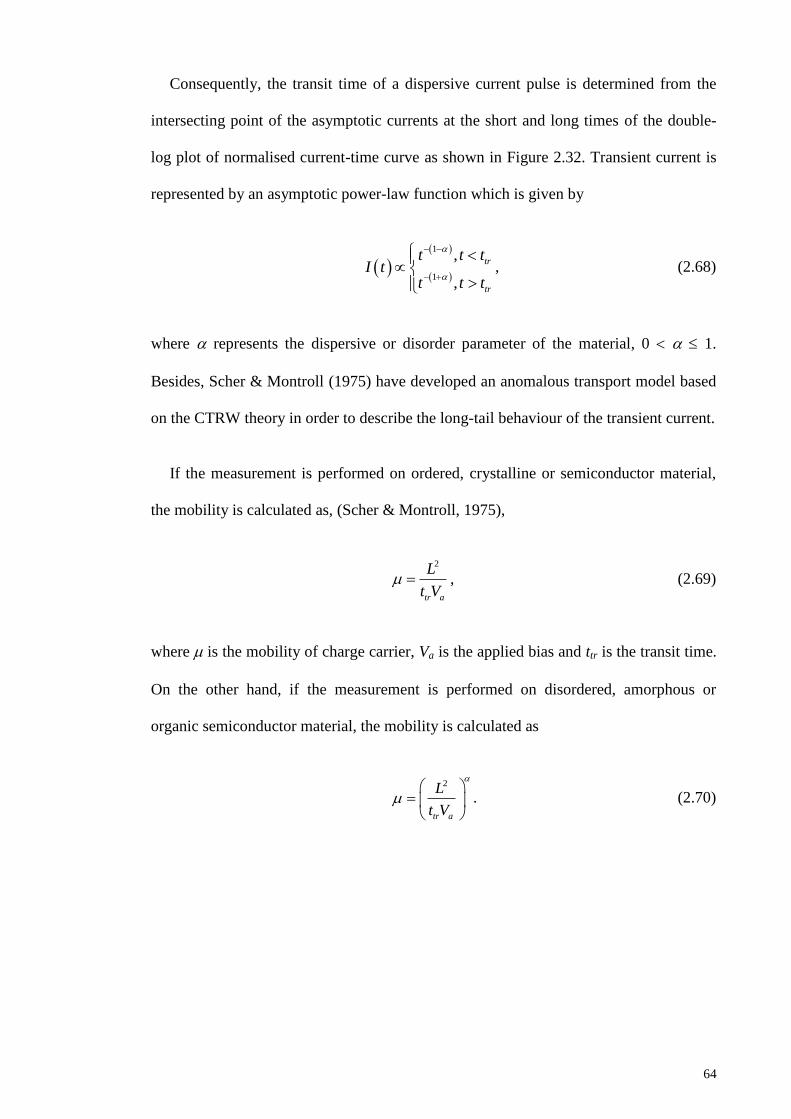
64

Consequently, the transit time of a dispersive current pulse is determined from the

intersecting point of the asymptotic currents at the short and long times of the double-

log plot of normalised current-time curve as shown in Figure 2.32. Transient current is

represented by an asymptotic power-law function which is given by

1

1

,

,

tr

tr

t t tI t

t t t

, (2.68)

where represents the dispersive or disorder parameter of the material, 0 1.

Besides, Scher & Montroll (1975) have developed an anomalous transport model based

on the CTRW theory in order to describe the long-tail behaviour of the transient current.

If the measurement is performed on ordered, crystalline or semiconductor material,

the mobility is calculated as, (Scher & Montroll, 1975),

2

tr a

L

t V , (2.69)

where is the mobility of charge carrier, Va is the applied bias and ttr is the transit time.

On the other hand, if the measurement is performed on disordered, amorphous or

organic semiconductor material, the mobility is calculated as

2

tr a

L

t V

. (2.70)

65

Figure 2.32: A double-log plot of transient photocurrent associated with a packet of

charge carriers moving in an electric field, with a hopping-time distribution function

(t) ~ t-1-

, 0 < < 1, towards an absorbing barrier at the sample surface. (Scher &

Montroll, 1975)

2.8.2 Continuous-time random walk theory

Scher and Montroll (1975) derived a continuous-time random walk model which

could explain the important features of the transient photocurrent measured by TOF

measurement in amorphous materials. The CTRW model assumes that (i) the transport

dynamic is a series of charge carrier (random walker) hopping from one localised site to

another empty site, (ii) each hopping event happens independently, (iii) the hopping

time, time interval between two successive hopping events, is an independent and

identically distributed (iid) random variable which is characterised by a hopping-time

distribution function that takes the form of a board power-law distribution, and (iv) the

hopping sites are distributed randomly and thus the structural and energy disorder of the

material are incorporated into the board power-law distribution.

CTRW process is described by the generalised master equation for PDF of just

arriving at position x at time t from x’ and t’ (Metzler & Klafter, 2000c, 2004),

0

, ' ', ' ', ' 'x t dx x t x x t t dt x t

, (2.71)

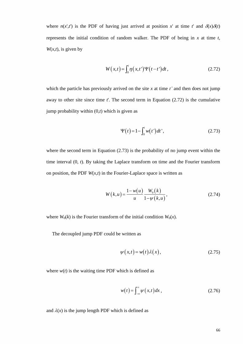
66

where n(x',t') is the PDF of having just arrived at position x' at time t' and (x)(t)

represents the initial condition of random walker. The PDF of being in x at time t,

W(x,t), is given by

0

, , ' 't

W x t x t t t dt , (2.72)

which the particle has previously arrived on the site x at time t’ and then does not jump

away to other site since time t'. The second term in Equation (2.72) is the cumulative

jump probability within (0,t) which is given as

0

1 ' 't

t w t dt , (2.73)

where the second term in Equation (2.73) is the probability of no jump event within the

time interval (0, t). By taking the Laplace transform on time and the Fourier transform

on position, the PDF W(x,t) in the Fourier-Laplace space is written as

01

,1 ,

w u W kW k u

u k u

, (2.74)

where W0(k) is the Fourier transform of the initial condition W0(x).

The decoupled jump PDF could be written as

,x t w t x , (2.75)

where w(t) is the waiting time PDF which is defined as

,w t x t dx

, (2.76)

and (x) is the jump length PDF which is defined as

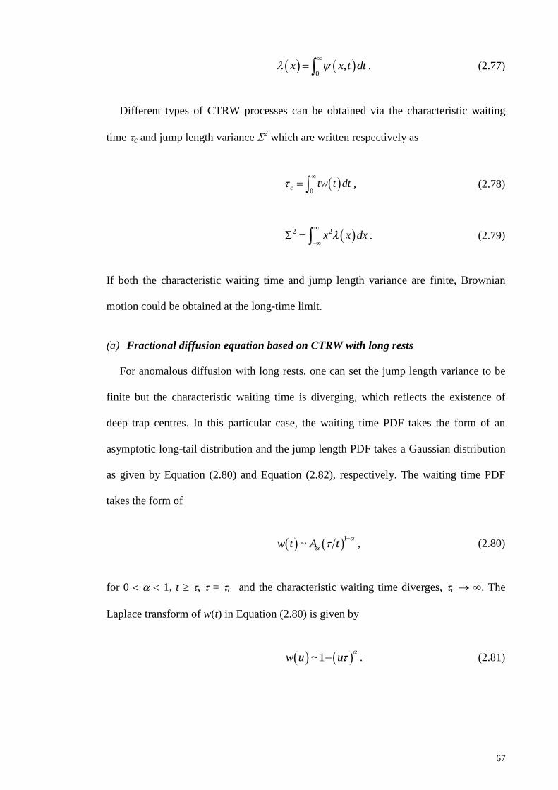
67

0

,x x t dt

. (2.77)

Different types of CTRW processes can be obtained via the characteristic waiting

time c and jump length variance 2 which are written respectively as

0

c tw t dt

, (2.78)

2 2x x dx

. (2.79)

If both the characteristic waiting time and jump length variance are finite, Brownian

motion could be obtained at the long-time limit.

(a) Fractional diffusion equation based on CTRW with long rests

For anomalous diffusion with long rests, one can set the jump length variance to be

finite but the characteristic waiting time is diverging, which reflects the existence of

deep trap centres. In this particular case, the waiting time PDF takes the form of an

asymptotic long-tail distribution and the jump length PDF takes a Gaussian distribution

as given by Equation (2.80) and Equation (2.82), respectively. The waiting time PDF

takes the form of

1

~w t A t

, (2.80)

for 0 1, t , = c and the characteristic waiting time diverges, c . The

Laplace transform of w(t) in Equation (2.80) is given by

~1w u u

. (2.81)

68

The jump length PDF takes the form of

2

22

1exp

44

xx

, (2.82)

where 22 =

2 is the jump length variance and its Fourier transform is given by

2 2 4~1 +Ok k k . (2.83)

By using Equation (2.81) and Equation (2.83) in Equation (2.74), thus, the PDF

W(x,t) in Fourier-Laplace space is written as

0

2,

1

W k uW k u

K u k

, (2.84)

where K = 2/2

is the anomalous diffusion coefficient with unit of cm2s

-. By using

the following identities,

0 tL D f t u f u , (2.85)

2 2 2F d f x dx k f k , (2.86)

and obtaining the inverse Laplace and Fourier transforms of W(x,t), one obtains the

integral form of the FDE (Barkai et al., 2000; Metzler & Klafter, 2000c) as

2

0 0 2, ,RL

tW x t W x D K W x tx

. (2.87)

Differentiate W(x,t) with respect to time, W(x,t)/t, the differential form of the FDE

(Wyss, 1986) is resulted as

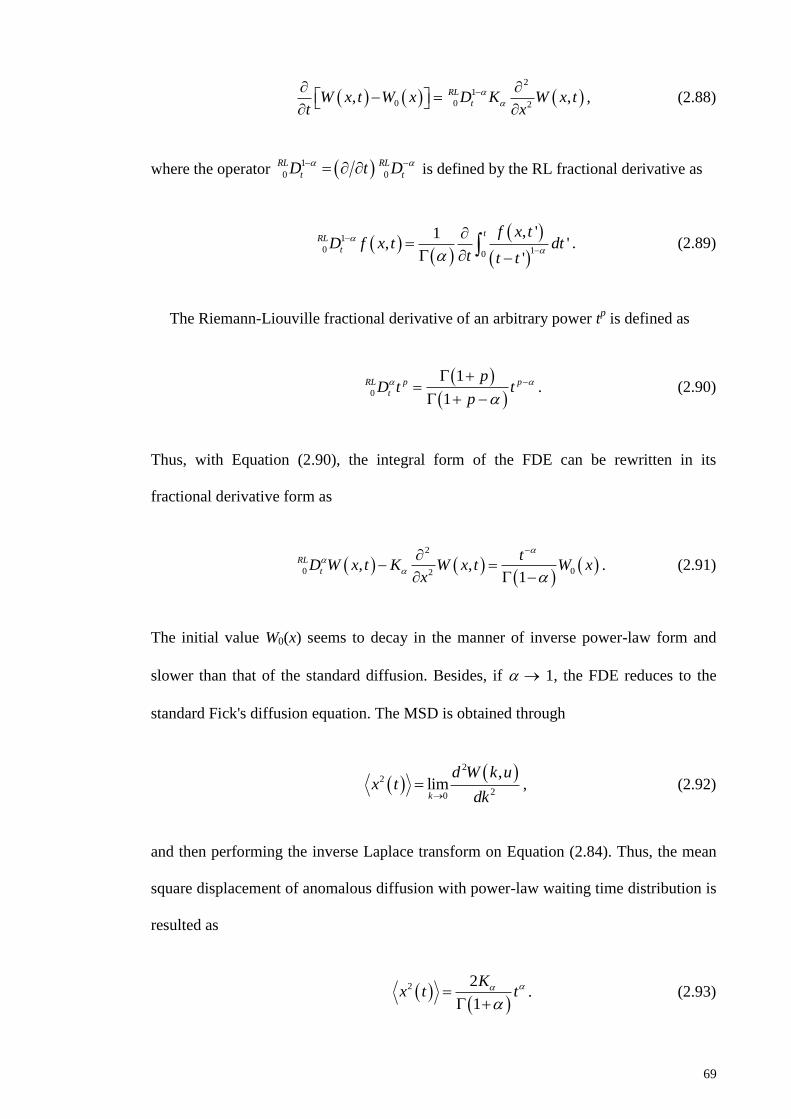
69

2

1

0 0 2, ,RL

tW x t W x D K W x tt x

, (2.88)

where the operator 1

0 0

RL RL

t tD t D is defined by the RL fractional derivative as

1

0 10

, '1, '

'

tRL

t

f x tD f x t dt

t t t

. (2.89)

The Riemann-Liouville fractional derivative of an arbitrary power tp is defined as

0

1

1

RL p p

t

pD t t

p

. (2.90)

Thus, with Equation (2.90), the integral form of the FDE can be rewritten in its

fractional derivative form as

2

0 02, ,

1

RL

t

tD W x t K W x t W x

x

. (2.91)

The initial value W0(x) seems to decay in the manner of inverse power-law form and

slower than that of the standard diffusion. Besides, if 1, the FDE reduces to the

standard Fick's diffusion equation. The MSD is obtained through

2

2

20

,limk

d W k ux t

dk , (2.92)

and then performing the inverse Laplace transform on Equation (2.84). Thus, the mean

square displacement of anomalous diffusion with power-law waiting time distribution is

resulted as

2 2

1

Kx t t

. (2.93)

70

(b) Fractional diffusion equation based on CTRW with Lévy flights

For diffusion with Lévy flights (long jumps), one can set the jump length variance to

be diverging but the characteristic waiting time is finite. This diffusion has Markovian

behaviour due to the finiteness of the characteristic waiting time. In this case, the

waiting time PDF takes a Poisson distribution and the jump length PDF takes a Lévy

distribution with the asymptotic behaviour as given by Equation (2.94) and Equation

(2.96), respectively. The waiting time PDF is defined as (Metzler & Klafter, 2000c),

1

expw t

t , (2.94)

where = c and its Laplace transform is given by

2~1w u u . (2.95)

The jump length PDF takes the asymptotic form of

1

s

ss

Ax

x

, (2.96)

for 1 s 2, x and its Fourier transform is given by

11

exp

ss

ss

k kk

. (2.97)

By using Equation (2.95) and Equation (2.96) in Equation (2.74), thus, the PDF

W(x,t) in Fourier-Laplace space is written as

1

,ss

W k uu K k

, (2.98)

71

where s sK is the anomalous diffusion coefficient with unit of sα -1cm s . By

performing inverse Fourier transform and then Laplace transform, the space-fractional

diffusion equation due to Lévy flight is obtained as

,s sW

x

WK D W x t

t

, (2.99)

where sW

xD

is the Weyl fractional differential operator in one dimension which is same

as the Riesz fractional differential operator. Equation (2.99) could be solved using the

Fox function. Figure 2.33 shows the comparison of the trajectories of a Brownian

motion and Lévy flight with fractal dimension Df = 1.5 for about 7000 steps. The Lévy

flight can be viewed as a local motion sporadically interrupted by a long break on all

length scales which leads to the formation of clustering of trajectory before a long jump

occurs. The trajectory of Lévy flight could also be characterised by the fractal

dimension.

Figure 2.33: Comparison between the trajectories of Brownian motion (left) and Lévy

flight at Df = 1.5 (right) for about 7000 steps. (Metzler & Klafter, 2000c)

72

(c) Fractional diffusion equation based on CTRW with long rests and Lévy flights

When both the characteristic waiting time and jump length variance become infinite,

the propagation of a random walker is characterised through broad PDFs and the space-

time fractional diffusion equation would be resulted as (Metzler & Klafter, 2000c),

1

0 ,s sRL W

t x

WD K D W x t

t

, (2.100)

where s sK

, sW

xD

is the RL time-fractional differential operator and sW

xD

is

the Weyl space-fractional differential operator. The pseudo MSD is defined as

22 s

Lx t t

, (2.101)

which indicates that particle spreads finitely in a space in a given time interval.

(d) Fractional Langevin equation

Fractional Langevin equation is generalised from the LE to take into account for the

damping effect due to an additional frictional force, which depends on the memory of

the particle acceleration, to the Stokes drag force. The additional frictional force is

called the Basset force (Basset, 1888; Mainardi & Pironi, 1996) and is given by

0 0

9 1 1

2 FLE FLE FLE

F m t B t

, (2.102)

where (t) is velocity of particle, m is the mass of particle,

2

0 , ,pa

FLE FLE

f

r

(2.103)

is the viscosity of the liquid, ra is the radius of the particle, p is the density of

particle, f is the density of liquid and B(t) is given as

73

0

1 1:

1 2

t td t ds d t dsB t ds ds

t s t s

. (2.104)

By using the RL fractional derivative of order ½, Equation (2.104) can be rewritten

as

3/2

1/2

02

RL

t

tB t D t t

. (2.105)

Thus, the FLE is resulted as

1/2

0 0

1 11 RL

FLE t

e e

d tD t R t

dt m

, (2.106)

where R(t) is the random fluctuating force and the damping effect of the frictional force

is given by the new friction coefficient as

3/2

0

1

2FLE FLE

e

tt t

, (2.107)

with an additional fractional noise associated to the term t3/2

in addition to the white

noise in the standard LE. The mobility of the particle is written as

FLE e

em m

, (2.108)

where

0

0

1 9 26 , ,

2 9a f FLE FLE FLE

FLE FLE

mr

(2.109)

and 1 FLE LE m is the friction coefficient per unit mass.

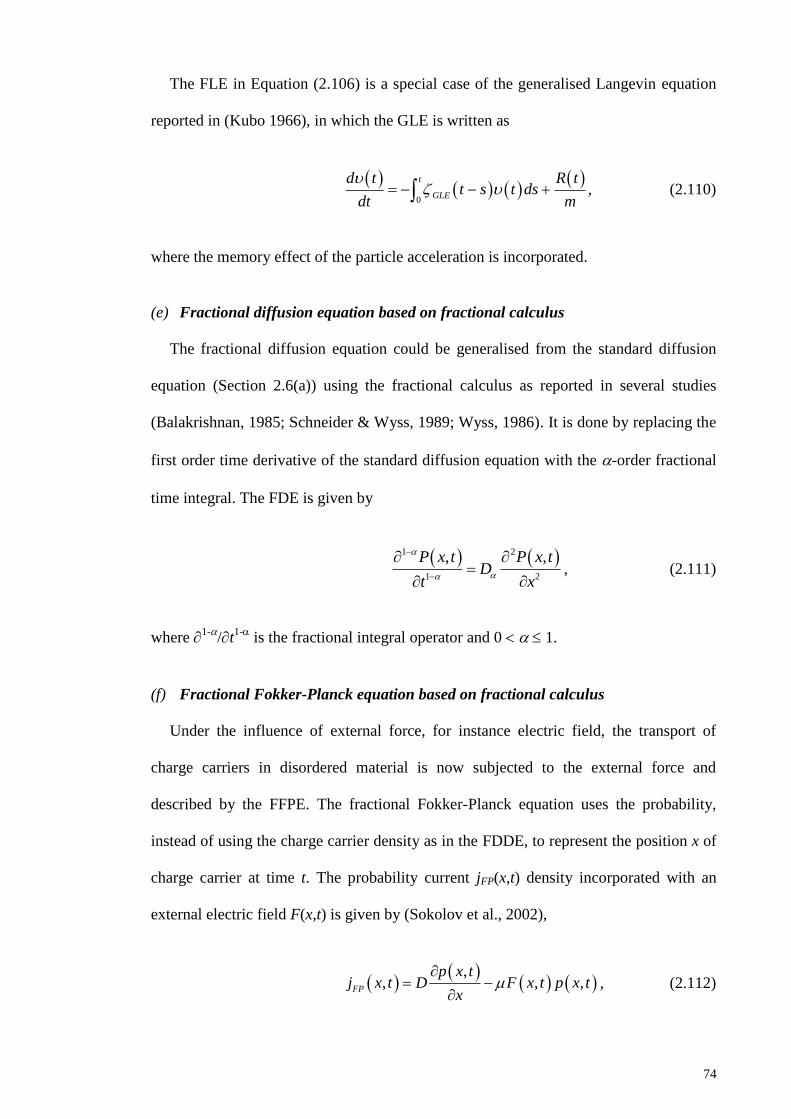
74

The FLE in Equation (2.106) is a special case of the generalised Langevin equation

reported in (Kubo 1966), in which the GLE is written as

0

t

GLE

d t R tt s t ds

dt m

, (2.110)

where the memory effect of the particle acceleration is incorporated.

(e) Fractional diffusion equation based on fractional calculus

The fractional diffusion equation could be generalised from the standard diffusion

equation (Section 2.6(a)) using the fractional calculus as reported in several studies

(Balakrishnan, 1985; Schneider & Wyss, 1989; Wyss, 1986). It is done by replacing the

first order time derivative of the standard diffusion equation with the -order fractional

time integral. The FDE is given by

1 2

1 2

, ,P x t P x tD

t x

, (2.111)

where 1-

/t1-

is the fractional integral operator and 0 1.

(f) Fractional Fokker-Planck equation based on fractional calculus

Under the influence of external force, for instance electric field, the transport of

charge carriers in disordered material is now subjected to the external force and

described by the FFPE. The fractional Fokker-Planck equation uses the probability,

instead of using the charge carrier density as in the FDDE, to represent the position x of

charge carrier at time t. The probability current jFP(x,t) density incorporated with an

external electric field F(x,t) is given by (Sokolov et al., 2002),

,

, , ,FP

p x tj x t D F x t p x t

x

, (2.112)

75

where P(x,t) is the probability of finding charge carrier at x and time t, D is the diffusion

coefficient and is the mobility. Substitute Equation (2.112) in the continuity equation,

one gets the FPE as

2

2

, ,, ,

p x t p x tD F x t p x t

t x x

. (2.113)

By using the RL fractional derivative, one can generalise the FPE equation to the

FKKE as

21

1 2

, ,, , 0

p x t p x tF x t p x t D

t t x x

, (2.114)

where D and are the fractional diffusion coefficient and fractional mobility,

respectively. The ratio of D/ = kBT gives the generalised Einstein's relationship.

76

CHAPTER 3: RESEARCH METHODOLOGY

Organic field-effect transistors based on P3HT are fabricated in order to obtain the

transient current noise for scaling analysis. Hence, this chapter provides some details on

the fabrication and electrical characterisations of OFET. The fractal analysis methods

which will be used to analyse the transient current noise are documented herein.

Anomalous charge transport theory incorporated with multiple-trapping which is

deduced using the fractional calculus and the numerical methods used to solve the

transport equations are demonstrated in this chapter. Lastly, transient current calculation

and simulation procedures of charge transport are presented.

3.1 Fabrication of organic field-effect transistor and current-voltage

measurement

Top-contact and bottom-gate OFETs were fabricated in order to study charge carrier

transport dynamics through their behaviour of noise. A 100 nm thick SiO2 layer is

grown on top of an n-type silicon substrate to serve as the dielectric layer. The active

layer of the device is made of P3HT. P3HT is dissolved in chloroform and is spin-

coated on top of the dielectric layer. The structure of the P3HT OFET is depicted in

Figure 3.1. P3HT is chosen in this study simply due to its high charge carrier mobility

and commercial availability. The P3HT active layer is thermally treated at 120 C for

ten minutes. The source and drain electrodes are deposited with a 50 nm thick gold on

top of the P3HT active layer. The channel width (arranged in interdigitated design) and

length are 11.2 mm and 40 µm, respectively.

77

Figure 3.1: Top-contact and bottom-gate P3HT OFET structure and setup of current-

voltage measurement.

Two Keithley SMUs are connected to the source, drain and gate contacts of the

OFET as shown in Figure 3.1. The drain currents are then measured for source-drain

voltage ranging from 0 to 60 V with respect to different gate voltages in order to

obtain the current-voltage characteristic of the OFET. Low noise coaxial cable is used to

minimise the triboelectric noise which is induced from the relative movement between

the dielectric and shielding layers of the cable. The measurement setup is placed in a

grounded metal box so that it is shielded from the electromagnetic interference radiating

from open space. Since the device is biased and measured using SMUs, thus power line

noise is superimposed on the noise of the SMUs which yields a sub-nanoampere noise

floor. Nevertheless, the current measured from the devices are ranging from

microamperes to sub-miliamperes, hence the noise floor of SMUs is insignificant as

compared to the currents resulted from devices. Activation energy of P3HT organic

semiconductor with low mobility (~10-4

cm2/Vs) is around 300 meV (Craciun, 2011),

thus thermal noise generation at room temperature could be negligible during the

measurement.

78

3.2 Low-frequency noise measurement

Low-frequency noise measurement is a common technique used to characterise the

noise behaviour and reliability of a device. This is because this technique is sensitive

enough to probe the microscopic properties, such as the surface defects, interface

defects, bulk defects and generation-recombination centres, of a device. Figure 3.2

shows a setup for the low-frequency noise measurement which consists of a current

amplifier, a dynamic signal analyser or a power spectrum analyser, a digital multimeter,

an oscilloscope and one or two source-measurement unit(s). The current amplifier is

used to amplify the current noise resulted from the DUT and then feeds it into the DSA.

Power spectral density of the current noise is computed in the DSA and then recorded in

a personal computer. The current noise is also measured with a DMM and monitored by

an OSK during the measurement. For very low current level measurement, a pre-

amplifier is connected between the DUT and the current amplifier to sense and pre-

amplify the low current which is resulted from the DUT before it is fed into the current

amplifier.

Figure 3.2: System for measuring low-frequency noise. (Kasap & Capper, 2006)

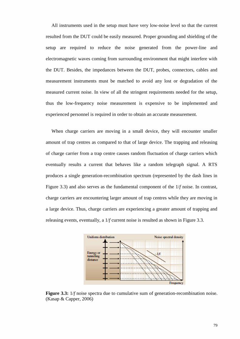
79

All instruments used in the setup must have very low-noise level so that the current

resulted from the DUT could be easily measured. Proper grounding and shielding of the

setup are required to reduce the noise generated from the power-line and

electromagnetic waves coming from surrounding environment that might interfere with

the DUT. Besides, the impedances between the DUT, probes, connectors, cables and

measurement instruments must be matched to avoid any lost or degradation of the

measured current noise. In view of all the stringent requirements needed for the setup,

thus the low-frequency noise measurement is expensive to be implemented and

experienced personnel is required in order to obtain an accurate measurement.

When charge carriers are moving in a small device, they will encounter smaller

amount of trap centres as compared to that of large device. The trapping and releasing

of charge carrier from a trap centre causes random fluctuation of charge carriers which

eventually results a current that behaves like a random telegraph signal. A RTS

produces a single generation-recombination spectrum (represented by the dash lines in

Figure 3.3) and also serves as the fundamental component of the 1/f noise. In contrast,

charge carriers are encountering larger amount of trap centres while they are moving in

a large device. Thus, charge carriers are experiencing a greater amount of trapping and

releasing events, eventually, a 1/f current noise is resulted as shown in Figure 3.3.

Figure 3.3: 1/f noise spectra due to cumulative sum of generation-recombination noise.

(Kasap & Capper, 2006)

80

An alternative method is proposed in this work to analyse the current noise using its

time domain which requires much simple and cheaper measurement setup. Two

Keithley 236 SMUs, represented by the battery symbol as shown in Figure 3.4, are used

to bias the device and measure the current resulted from the device, where one unit of

the SMUs is used to establish the source-drain voltage Vds and measure the drain current

Ids while another unit of SMU is used to supply the gate voltage Vg and measure the gate

current Ig. In order to obtain the temporal evolution of (transient) currents, devices are

repetitively biased using the sweep function of the SMU while the resulted currents are

measured during a fast integration time of 416 s. The measured currents in time

domain are then stored in the buffer (maximum of 1000 readings) of the SMUs before

they are recorded in a desktop computer for subsequent noise analysis using the

conventional PSD method and the more robust DFA approach. Power spectral density

of the transient current is numerically computed by taking the squared modulus of fast-

Fourier transform of the transient current. This can be effortlessly done with the FFT

subroutine available in the MATLAB program.

Figure 3.4: Current noise analysis based on PSD method and DFA.

81

3.3 Fractal analysis of current noise

This section provides the description of the fractal analysis method, namely power

spectral density method and detrended fluctuation analysis, used to analyse the current

noises of OFET measured at various source-drain voltages.

3.3.1 Power spectral density method

The low frequency noise analysis using the power spectra density method is

implemented by computing the squared modulus of Fourier transformed of the

measured transient current noise. If a time series exhibits power-law scaling the PSD

would take the following form

1

~PS

S ff , (3.1)

where S(f) is the power spectral density and f is the frequency.

The slope of the log-log plot of the PSD yields the scaling exponent PS. One can

link the scaling exponent PS to the Hurst exponent H if the underlying transport

mechanism is described by the FBM. The scaling exponent PS gives useful information

of the transport dynamics of the charge carriers hopping in the organic or polymer

material of OFETs and also information on trap centres and defects. The presence of

trap centres and defects could induce generation-recombination noise and 1/f noise in

the devices that sets a maximum limit on the performance of the devices (Jurchescu et

al., 2008; Ke et al., 2006, 2008; Xu et al., 2010). The occurrence of 1/f noise in a device

could be observed at the low frequency region of the current noise PSD in which the

PSD is inversely proportional to the frequency. In addition, it has been demonstrated in

(Brophy, 1968, 1969; Huo et al., 2003; Nelkin & Harrison, 1982) that the nonstationary

effect is naturally present in the current noise despite of the influence of the finite

82

sampling size effect of the time series. Huo et al. (2003) has also shown that the power

spectrum of the current noise follows a fractal power-law scaling or 1/f type behaviour

in which the scaling exponent of the power spectrum varies in the range of 1 < PS < 2.

This is associated to the density of trap centres and the probability distribution of release

rates that varies slowly with frequency (Nelkin & Harrison, 1982). The relationship of

the scaling exponent PS and the Hurst exponent is given as PS = 2H + 1.The current

noise can also be classified as uncorrelated white noise when PS = 0 (H = 0.5), 1/f

noise (H = 0) and Brownian noise when PS = 2 (H = 0.5).

3.3.2 Detrended fluctuation analysis

The detrended fluctuation analysis is a statistical method that has been developed to

study the existence of short-rage or long-range correlation of time series. This method

was first used to study DNA sequences (Peng et al., 1994) and progressively found its

applications in other time series analysis such as that of the electrocardiogram analysis

(Huikuri et al., 2009; Meyer & Stiedl, 2003; Peng et al., 1995), electroencephalogram

analysis (Ignaccolo et al., 2010; Lee et al., 2004; Penzel et al., 2003), weather

forecasting (Matsushita et al., 2007) and electrical noise study in semiconductor devices

(Houssa et al., 1998; Shiau, 2011). Detrended fluctuation analysis has been proven to be

a robust technique in time series analysis due to the capability of detecting whether a

trend is superimposed on a time series (Hu et al., 2001) and the capability of

differentiating stationary and nonstationary properties inherent in a time series (Chen et

al., 2002). This method contains few important steps (Peng et al., 1994, 1995; Penzel et

al., 2003) as outlined in the following paragraphs. As shown in the Figure 3.5, the time

series x(i) is first subtracted from the mean value x and then integrated as given by,

1

j

i

Y j x i x

. (3.2)

83

Figure 3.5: Detrending procedure of DFA at different window sizes. (Penzel et al.,

2003)

The integrated time series Y(j) is then divided into boxes of equal length nDFA. The

next step involves fitting a linear least-squares line in each box of length nDFA in which

it reflects the local trend in that box and its y-coordinate of the local trend is represented

by Yfit(j). The integrated time series Y(j) is then detrended via subtracting it from the

local trend Yfit(j) of each box. The average fluctuation F(nDFA) or the root-mean square

of the difference between Y(j) and Yfit(j) is computed as

2

1

1 N

DFA fit

j

F n Y j Y jN

, (3.3)

where N is the length of the time series. The average fluctuation F(nDFA) is then re-

calculated for all box sizes leading to the power-law behaviour, DFA

DFA DFAF n n

, if x(i)

is a fractal noise. As shown in Figure 3.6, the slope of linear scaling regime of the log-

log plot of F(nDFA) versus nDFA gives the scaling exponents DFA which can then be used

to deduce the correlation behaviour of fractal noises.

84

Figure 3.6: Double-log plot for r.m.s. fluctuation F versus box size. (Penzel et al.,

2003)

One can link the scaling exponent DFA to the anomalous diffusion process such as

the fractional Brownian motion where DFA = H + 1. When DFA = 0.5, the integrated

time series is associated with random walk whose original time series does not present

any correlation between two events. This is the standard characteristic of white noise.

The time series is said to be persistent with long memory effect when 0.5 DFA 1.

On the other hand, anti-persistent time series exhibits short memory effect and in this

case, 0 DFA 0.5. If DFA = 1 (H = 0), time series is identified as having the

characteristic of 1/f noise. Finally, when = 1.5 (H = 0.5), the integrated time series is

considered as a Brownian noise.

3.4 Transport equation based on fractional calculus

This section provides the description of the transport equation used in this work to

model the anomalous transport in disordered organic semiconductor and the numerical

techniques used to obtain the solutions of the transport equation.

3.4.1 Fractional kinetic equation with multiple-trapping mechanism

Based on multiple-trapping model, photo-generated charge carriers in disordered

material are classified into trap (localised) and free (delocalised) charge carriers. Trap

85

charge carrier is the charge carrier which is captured in localised state and free charge

carrier is the charge carrier which is freely hopping from one trap centre (localised state)

to another trap centre. The movement of free charge carriers is subjected to phonon

scatterings and external electric field that cause the charge carriers to drift with a finite

average velocity. The capture rate of charge carrier into the localised state is linearly

proportional to the number of free charge carrier density. Trap charge carrier density is

assumed to be higher than the free charge carrier density and the average time of

delocalisation is approaching zero, 0 0. The total charge carrier density, p(x,t) is the

sum of the trap, pt(x,t), and free, pf(x,t), charge carrier densities at x and t which is given

as

p(x,t) = pt(x,t) + pf(x,t). (3.4)

As demonstrated in (Sibatov & Uchaikin, 2007, 2009), the relationship between the

time rate of change of trap and free charge carrier densities, derived based on an

asymptotically power-law distribution function for the random residence time in the

localised states, is given as

1 ,

00

, 1

1

ft p x st

t s

p x tc ds

t t

1

0

,, ftp x tp x t

ct t

, (3.5)

where t is the RL fractional derivative of order 0 < < 1 which is an integral-

differential operator (Podlubny, 1998).

In the present of an applied electric field, the one-dimensional continuity equation of

the free charge carrier is given as

86

0

2

2

, ,1, ,

,,0 ,

f f

f

f

p x t p x tF x t p x t

t c t x

p x tD p x t

x

(3.6)

where p(x,0)(t) is the initial photo-generated charge carriers. By assuming that most of

the charge carriers are trapped in the localised states, p(x,t) pt(x,t), and substituting

Equation (3.5) into Equation (3.6), one could rewrite Equation (3.6) for the continuity

equation of the total charge carrier density as

21

0 01 2

, ,, , ,0 .

p x t p x tc F x t p x t c D p x t

t t x x

(3.7)

By applying RL fractional integral operator of order 1 to Equation (3.7), the

continuity equation of the total charge carrier density can be written as

2

2

, ,, , ,0 ,

1

p x t p x t tK x t p x t D p x

t x x

(3.8)

where K(x,t) = cl = c

0F(x,t) is the anomalous advection coefficient, D = 0cD is

the anomalous diffusion coefficient, 0 is the average time of delocalisation (mean free

time of a charge carrier moving between two successive entrapments), l = 0F(x,t) is

the average length of delocalisation, is the mobility and D is the diffusion coefficient

that is calculated using the Einstein relationship D = kBT/e where e is the electronic

charge, kB is the Boltzmann constant and T is the temperature. The velocity of charge

carrier is written as , ,v x t F x t where F(x,t) is the localised electric field. The

charge carrier capture coefficient 1

0 sinc

where 0 is the capture rate

of charge carriers into the localised states and = kBT/E0 is the dispersive parameter

which depends on the temperature T and the mean value E0 of the exponential energy

87

density of localised state of charge carrier. The dispersive parameter is also associated

to the fractional derivative order in Equation (3.5). The dispersive parameter, (x,t),

can also be expressed as a function of time, space or both time and space to represent

the change of material property (i.e. energy disorder) of inhomogeneous materials.

Thus, Equation (3.8) could be generalised to the one-dimensional variable-order time-

fractional drift-diffusion equation which is written as

, 2 ,

, , 2,

, ,, , ,0 ,

1 ,

x t x t

x t x tx t

p x t p x t tK x t p x t D p x

x x x tt

(3.9)

and representing the dispersive transport dynamics of charge carriers in organic

semiconductors based on the multiple-trapping mechanism. It should be noted that the

propagation of charge carriers will resemble the normal transport dynamics when (x,t)

is approaching 1.

It is known that the RL fractional derivative can be approximated using the GL

fractional derivative in order to obtain the numerical solutions of the time-fractional

diffusion equation as demonstrated in (Podlubny, 1998; Yang et al., 2009). However,

the order of accuracy of the GL fractional derivative is below one and shifted version of

the GL fractional derivative should be used in order to obtain stable solutions as pointed

in (Sousa, 2012). Murio (2008b) also pointed out that the GL fractional derivative might

only be consistent at all values of x and coincides with the Caputo fractional derivative

if zero initial condition is fulfilled.

Nevertheless, several works (Lin & Xu, 2007; Murio, 2008a; Sun et al., 2012) had

demonstrated a finite difference scheme to discretise the Caputo time fractional

derivative and able to obtain unconditionally stable solutions for the time-fractional

diffusion equation with (2) order accuracy in time. Solutions of the Caputo time-

88

fractional diffusion equation are obtained through the integer order derivatives at all

previous time steps. Thus, finite difference method used to discretise the integer order

derivative could be readily adopted to discretise the Caputo time fractional derivative.

This allows the past events of transport dynamics of charge carriers at all previous time

steps to be naturally incorporated in the Caputo time fractional derivative. Besides,

physical conditions could be represented by the boundary conditions of the Caputo

time-fractional drift-diffusion equation. It is also known that the Caputo fractional

derivative of a constant is zero but not the case for the RL fractional derivative.

3.4.2 Electric potential and field

The electric potential V(x,t) is obtained via solving the self-consistent Poisson

equation as given below,

2

20

, ,

r

V x t x t

x

, (3.10)

where (x,t) = ep(x,t) is the charge density, r is the relative permittivity of the material

and 0 is the permittivity of vacuum. The localised electric field is then calculated as,

,

,V x t

F x tx

. (3.11)

3.4.3 Current density

The average current density IT(t) is defined as the conduction current density

averaged over the thickness of the device or TOF cell,

0

,L

T

e dI t x L p x t dx

L dt , (3.12)

where p(x,t) is the total charge carrier density obtained by solving Equation (3.8) or

Equation (3.9). Observe that current density is generally inversely related to the cell

89

thickness L. Consequently, Equation (3.12) explicitly accounts for the influence of the

film thickness in that the current density level decreases when the thickness of the film

increases and vice versa.

3.5 Numerical methods

The anomalous transport dynamics of charge carriers in organic semiconductor

materials are studied by using the fractional drift-diffusion equation derived based on

the multiple-trapping mechanism (Sibatov & Uchaikin, 2009; Uchaikin & Sibatov,

2008, 2013). The integer order space derivative, integer time derivative and fractional

time derivative are approximated by using the finite difference method as described in

the subsequent sub-sections.

3.5.1 Finite difference scheme for integer order differential operator

The derivative of a function f(x) at x, based on the First Principle definition, is

defined as

'

0limh

f x h f xf x

h

, (3.13)

where h = x is the interval between x and x + h (Burden & Faires, 2011). Due to the

rounding-off error, two-point difference formula has an error of 22h f and lies

between x and x + h. In general, it is recommended that using more points in the

approximation of the derivative of f(x) could improve the accuracy of the

approximation. Thus, the three-point midpoint (central difference) formula for the first

derivative, with equally space point, is written as

2

3' 1

2 6

hf x f x h f x h f

h , (3.14)

90

where lies between x h and x + h. By expanding the function f(x) about a point x to

the third Taylor polynomial and evaluate at x h and x + h, the three-point midpoint

formula for the second derivative of f(x) can be defined as

2

4''

2

12

12

hf x f x h f x f x h f

h , (3.15)

where lies between x h and x + h. Equation (3.14) and Equation (3.15) can also be

used for time variable t.

3.5.2 Finite difference scheme for fractional order differential operator

In view of the advantages offered by the Caputo fractional time derivative, thus the

fractional time derivative in Equation (3.9) is expressed by using the Caputo fractional

time derivative which is defined, for a function f(x,t), as

,

, ,0

( , ) 1 ( , ), 0 ( , ) 1.

(1 ( , )) ( )

x tt

x t x t

f x t f x s dsx t

x t st t s

(3.16)

The variable-order Caputo fractional time derivative is discretised by using the

implicit difference scheme due to its unconditional stable property. Let’s define the

position is xi = ix for 0 i Nx, time is tk = kt for 0 k Nt 1, spatial step is x =

L/Nx, time step is t = T/Nt, T is the total time, L is the device length, Nt is the total time

step and Nx is the total spatial step. We can use the notation of

, ,i

k

i kf x t f i x k t f to represent the approximation of an arbitrary function and

i

k is fractional derivative order.

The variable-order fractional time differential operator, Equation (3.16), is

approximated as (Lin & Xu, 2007; Sun et al., 2012),

91

11

1 1

,

1

, ,1 0 1

, ,1

1 ,

i km

i k i km

x t k ti k i

x t x tti k m k

f x t f x s ds

sx tt t s

(3.17)

1

1

1

110

1

1

m

kim

m mk ti i

k t kmi

f f dsO t

t t s

.

1

1

11 , 1

10

1

2

ki

ki

k m k mki iα k m k

i ikmi

f fL f b

t

. (3.18)

where

1 11 1, 1 1 0 1 ,

k ki im k

ib m m , m , ,...,k

(3.19)

and 0, 1 1k

ib , , 1 0m k

ib as m and O(t) is the approximation error. It should be

noted that the results of the integer order time derivative of f(x,t) at all the previous time

steps are needed in order to implement the Caputo fractional derivative

3.5.3 Numerical integration

The definite integration of a function f(x) in a close interval [a, b] is given by

Riemann sum as

11

1

lim2

Nbi i

i ia N

i

x xf x dx f x x

, (3.20)

where f(x) is arbitrary function of x, xi is the i-th

point on the curve, and N is the total

number of points. When N , the R.H.S. of Equation (3.20) approximates the value

of the definite integral of f(x) over [a, b].

The most basic numerical integration method is carried out by approximating the

area under a curve over an interval [a, b] using a trapezoid as depicted in Figure 3.7.

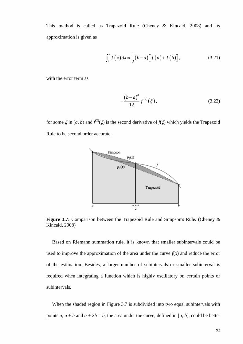
92

This method is called as Trapezoid Rule (Cheney & Kincaid, 2008) and its

approximation is given as

1

2

b

af x dx b a f a f b , (3.21)

with the error term as

3

2

12

b af

, (3.22)

for some in (a, b) and f(2)

() is the second derivative of f() which yields the Trapezoid

Rule to be second order accurate.

Figure 3.7: Comparison between the Trapezoid Rule and Simpson's Rule. (Cheney &

Kincaid, 2008)

Based on Riemann summation rule, it is known that smaller subintervals could be

used to improve the approximation of the area under the curve f(x) and reduce the error

of the estimation. Besides, a larger number of subintervals or smaller subinterval is

required when integrating a function which is highly oscillatory on certain points or

subintervals.

When the shaded region in Figure 3.7 is subdivided into two equal subintervals with

points a, a + h and a + 2h = b, the area under the curve, defined in [a, b], could be better

93

approximated using Equation (3.23). This technique is called the basic Simpson's Rule

(Cheney & Kincaid, 2008).

43

b

a

hf x dx f a f a h f b , (3.23)

where the subinterval h = (b a)/2 with the error term as

5

4

180

b af

, (3.24)


() is the fourth derivative of f() which yields the Simpson's

Rule to be fourth order accurate.

If the interval [a, b] is further subdivided into Nh subintervals in which Nh is divisible

by 2, thus the width of each subinterval is obtained as h = (b a)/Nh and each point is

given as xi = a + ih for 0 i Nh. This gives the Composite Simpson's Rule (Cheney &

Kincaid, 2008) as

/2 ( 2)/2

1 1

4 2 1 2 23

h hN Nb

ai i

hf x dx f a f b f a i h f a ih

, (3.25)

with the error term as

4

4

180

b a hf

, (3.26)


() is the fourth derivative of f() which yields the Composite

Simpson's Rule to be fourth order accurate.

94

3.5.4 Discretisation for partial differential equation

The anomalous transport dynamic of charge carriers in organic semiconductors is

studied by using the time-fractional drift-diffusion equation which is a generalisation

form of the normal diffusion equation incorporated with drift term due to the applied

electric field. So, it is worthwhile to take a look at the numerical method which can be

used to obtain the solution of the normal diffusion equation. Diffusion equation is a

parabolic type PDE which is written as (Burden & Faires, 2011; Cheney & Kincaid,

2008),

2

2

, ,; 0 , 0,

f x t f x tD x L t

t x

(3.27)

where D is the diffusion coefficient and Equation (3.27) is subjected to the following

conditions

0, , 0, 0;

,0 , 0 .

f t f L t t

f x f x x L

(3.28)

Finite difference method can be simply implemented to obtain the numerical solution

of Equation (3.27). It is carried out by replacing the first order time derivative and

second order space derivative in Equation (3.27) by Equation (3.14) and Equation (3.15)

, respectively. The first order time derivative is approximated by using the backward

difference method because the implicit difference scheme is unconditionally stable.

Thus, a larger time step could be used to reduce the computation time and memory size

as compared to the (smaller) time step required by the forward difference method. The

second order space derivative is approximated by using the central difference scheme

because smaller error is resulted as compared to that of the two-point midpoint

difference schemes.

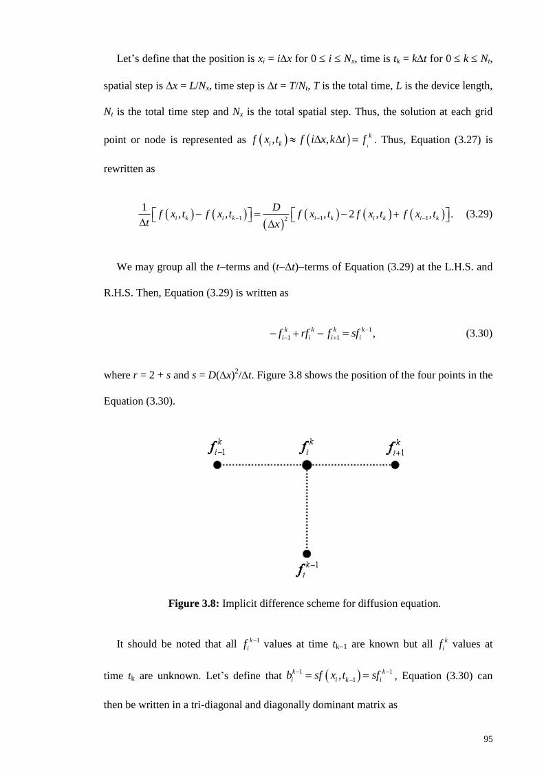
95

Let’s define that the position is xi = ix for 0 i Nx, time is tk = kt for 0 k Nt,

spatial step is x = L/Nx, time step is t = T/Nt, T is the total time, L is the device length,

Nt is the total time step and Nx is the total spatial step. Thus, the solution at each grid

point or node is represented as , ,i

k

i kf x t f i x k t f . Thus, Equation (3.27) is

rewritten as

1 1 12

1, , , 2 , , .i k i k i k i k i k

Df x t f x t f x t f x t f x t

t x

(3.29)

We may group all the tterms and (tt)terms of Equation (3.29) at the L.H.S. and

R.H.S. Then, Equation (3.29) is written as

1

1 1

k k k k

i i i if rf f sf

, (3.30)

where r = 2 + s and s = D(x)2/t. Figure 3.8 shows the position of the four points in the

Equation (3.30).

Figure 3.8: Implicit difference scheme for diffusion equation.

It should be noted that all 1k

if

values at time tk1 are known but all k

if values at

time tk are unknown. Let’s define that 1 1

1,k k

i i k ib sf x t sf

, Equation (3.30) can

then be written in a tri-diagonal and diagonally dominant matrix as

96

1 1

2 2

3 3

2 2

1 1

1

1 1

1 1

1 1

1 1

1

i i

n n

n n

f br

f br

f br

f br

f br

f br

, (3.31)

or rewritten as

Af = b . (3.32)

The unknown vector f can be solved because coefficient matrix A and R.H.S. vector

b are known. The linear equation system can be easily solved numerically by using the

Gaussian elimination method as described in the following subsection. The similar

numerical scheme will be implemented to obtain the solutions of the fractional time

drift-diffusion equation that represents the anomalous transport dynamic of charge

carriers in disordered organic semiconductors. The numerical procedure is described in

the section 3.5.6.

3.5.5 Gaussian elimination for solving linear equation systems

Many problems in science and engineering can be represented by a linear equation

system. Typically, the approximation of a parabolic PDE by algebraic equation often

produces a linear equation system which can be represented in a matrix form that has a

tri-diagonal structure,

97

1 1 1 1

1 2 2 2 2

2 3 3 3 3

1

2 1 1 1 1

1

i i i i i

n n n n n

n n n n

d c x b

a d c x b

a d c x b

a d c x b

a d c x b

a d x b

, (3.33)

where all the other elements in the coefficient matrix are zero, coefficients ai, bi, ci and

di are known variables and xj are unknown variables which will be determined.

Gauss elimination factorises the linear equation system (Ax = b) into an upper

triangular matrix U and a lower triangular matrix L, thus the coefficient matrix A is

rewritten as A = LU. The solution of the unknown vector x can be obtained from the

upper triangular matrix U after completing the procedures in the Gauss elimination

method. If the coefficient matrix A has specific form such as tri-diagonal, banded, or

symmetric structure, lesser amount of memory is required to store the elements of the

matrix. The conditions for the Gaussian elimination to be implemented and work

effectively are the matrix coefficient A is a matrix with size n n and do not have zero

triangular elements in matrix coefficient A.

The first phase in solving the unknown vector x is called the forward elimination

process where all the elements a of the matrix coefficient A will become zero (except a1

term), elements b and d will be replaced by new values and element c is unchanged.

11

1

; 2 .ii i i

i

ad d c i n

d

(3.34)

11

1

; 2 .ii i i

i

ab b b i n

d

(3.35)

98

Thus, the matrix in (3.33) is reduced to a non-zero upper triangular matrix and

written as

1 1 1 1

2 2 2 2

3 3 3 3

1 1 1 1

i i i i

n n n n

n n n

d c x b

d c x b

d c x b

d c x b

d c x b

d x b

, (3.36)

The second phase of the Gauss elimination is called the backward substitution

process. In this phase, the solution of xn in Equation (3.36) is obtained as

.nn

n

bx

d (3.37)

After that, the ithelement of vector x is obtained as

1

1; 1, 2,...,1.i i i i

i

x b c x i n nd

(3.38)

3.5.6 Discretisation for fractional drift-diffusion equation

Approximate the space derivative and fractional time derivative in Equation (3.9)

respectively by using the central difference scheme and Equation (3.18), thus the VO-

TFDDE can be rewritten as

1

1

, 2

1 1

2,

1 1

1 1

, ,

, ,, , .

i k

i k

x t

i k i k

x t

i k i k

i k i k

p x t p x tD

xt

p x t K x tK x t p x t

x x

(3.39)

99

1 1

1 1

1 1 11 1 1

0 2

1 1 1 11 11 1 1 1

0 0

2

.2 2

k ki i

k ki i

k k kα αk i i i

i

k k k kα αk ki i i i

i i

p p pL p c D

x

p p F Fc v c p

x x

(3.40)

The notations of , , , , i i i i i

k k k k kp v F V represent the approximations for the charge carrier

density, velocity, electric field, electric potential and disorder parameter (fractional

derivative order). Substitute Equation (3.18) into Equation (3.40) and group all the tk+1

and tk terms on the L.H.S. and R.H.S. of Equation (3.40), respectively. Equation (3.40)

is then written as

1 1

1 1

1 1

1

01 1 1 1

1 12

1 1

0 1 1

1 1

1 1 1

0 1 1 1

11, 1 , 1 1, 1 ,

1

22

2

2

2

2

1

k ki i

k ki i

k ki i

α k

ik k k k

i i i i

α k k

i i k k

i i

α k k k

i i i k

i

kk k m k m k k m k k

i i i i i i

m

c D tp p p p

x

c tp p

x

c t F Fp

x

b p b b p b

1 0.ip

(3.41)

By defining

1 11

01

, 2

2k ki iα k

ik

D i

c D tC

x

,

1 11 1

01

,

2

2

k ki iα k k

i ik

v i

c tC

x

and

1 1

1 1 1

0 1 11

,

2

2

k ki iα k k k

i i ik

F i

c t F FC

x

. The VOTFDDE is rewritten as

1 1 1 1 1 1 1 1 1

, , 1 , , , , 1

11, 1 , 1 1, 1 , 1 0

1

1 2

1 , 1.

k k k k k k k k k

D i v i i D i F i i D i v i i


i i i i i i i

m

C C p C C p C C p

b p b b p b p k

(3.42)

When k = 0 and 1 1k

i , Equation (3.42) resembles the standard drift-diffusion

equation.

100

1 1 1 1 1 1 1 1 1 0 0,1

, , 1 , , , , 11 2 , 1.D i v i i D i F i i D i v i i i iC C p C C p C C p p b (3.43)

Let’s define that 1 1 1

1 , ,

k k k

i D i v iP C C

, 1 1 1

, ,

k k k

i D i v iR C C , 1 1 1

, ,1 2k k k

i D i F iS C C and

1

1 1, 1 , 1 1, 1 , 1 0

1

1k

k k k m k m k k m k k

i i i i i i i i

m

Q b p b b p b p

. For k 1 and 1 i Nx – 1,

Equation (3.43) is a set of linear equations for 1k

ip that can be written in a matrix as

1 1 1 1

1 1 1 1

1 1 1 1 1

1 2 2 2 2

1 1 1 1 1

1

1 1 1 1

3 2 2 2

1 1 1

2 1 1

0 0

0

0

0 0

x x x x

x x x

k k k k

k k k k k

k k k k k

i i i i i

k k k k

N N N N

k k k

N N N

S R p Q

P S R p Q

P S R p Q

P S R p Q

P S p

1

2

1

1

x

x

k

N

k

NQ

, (3.44)

with the boundary conditions defined as p(0,t) = p(L,t) = 0.

The matrix in Equation (3.44) is a tri-diagonal matrix since the central three diagonal

elements on the L.H.S. of the matrix are non-zero. Forward elimination and backward

substitution method is adopted in order to solve the matrix in Equation (3.44) so that the

solutions 1

i

kp of the VO-TFDDE can be obtained. After the forward elimination

procedure, all the coefficient P are eliminated, all the coefficient R are remained and all

the new values of the ithelement of coefficient Q and S are calculated as:

1

1 1 1111

1

; 2 1.k

k k kii i i xk

i

PS S R i N

S

(3.45)

1

1 1 1111

1

; 2 1.k

k k kii i i xk

i

PQ Q Q i N

S

(3.46)

101

The matrix in Equation (3.44) is rewritten as

1 1 1 1

1 1 1 1

1 1 1 1

2 2 2 2

1 1 1 1

1 1 1 1

2 2 2 2

1 1 1

1 1 1

0 0

0

0

0 0

x x x x

x x x

k k k k

k k k k

k k k k

i i i i

k k k k

N N N N

k k k

N N N

S R p Q

S R p Q

S R p Q

S R p Q

S p Q

. (3.47)

In the backward substitution procedure, the first step is to obtain the solution 1

1

Nx

kp

from Equation (3.47) by

1

11

1 1

1

.x

x

x

k

Nk

N k

N

Qp

S

(3.48)

After that, the ithelement of

1

i

kp is obtained as

1 1 1 1

11

1; 1 2.k k k k

i i i i xk

i

p Q R p i NS

(3.49)

3.5.7 Discretisation for electric potential and Poisson equation

Electric field established within the device due to the present of charge carriers and

the external electric field could be calculated when the electric potential is obtained

through solving the Poisson equation which is an elliptical partial differential equation.

Thus, the numerical method used to solve the elliptic partial differential equation based

on finite difference method will be employed. It is done by replacing the second order

space derivative of the Poisson equation with the central difference scheme, thus

Equation (3.10) is written as

102

1 1 111 1

2

0

2.

k k kki i ii

r

V V V ep

x

(3.50)

At k, for k 1 and 1 i Nx – 1, Equation (3.50) is a set of linear equations for 1

i

kV

and can be written in a matrix as

1 101 021

1

1 1

2 2

2

1 1

0

1 1

2 2

1

1 11 01 2

2 1 0 0

1 2 1

0

1 2 1

0

1 2 1

0 0 1 2

x x

x

x x

k kr

k

k k

k k

i i

r

k k

N N

k

k kN rN N

p Ve xV

V p

e xV p

V p

Vp V

e x

,

(3.51)

where the boundary conditions are V(0,t) = Va (applied bias) and V(L,t) = 0. All the

values of the charge density 1

i

kep on the R.H.S. of the matrix are known for all grid

points. The matrix in Equation (3.51) is a tri-diagonal matrix since the central three

diagonal elements on the L.H.S. of the matrix are non-zero. Thus, the similar steps used

to obtain the solutions for the charge carrier density can also be used to solve for the

electric potential. After that, the ithelement of

1

i

kF is calculated using

1 1

1 1 1

2

k kk i i

i

V VF

x

. (3.52)

Electric fields at the terminals (boundaries) of the device are obtained as

1 1

1 1 00 ,

k kk V V

Fx

(3.53)

103

and

1 1

11 .x x

x

k k

N Nk

N

V VF

x

(3.54)

3.5.8 Discretisation for current density

By approximating the integration and the integer order time derivative in Equation

(3.12) respectively with the composite Simpson's Rule and the forward difference

method, the current density Ik+1

at time tk+1

can be written as

1 100 0

1

2 1 21 11 12 2 1

2 2 2 1 2 1

1 1

1 1

32 1 4 1

x x

k k k kLL L

k

N Nk kk k k ki ii i i i

i i

x xp p p p

L Le xJ

t x xp p p p

L L

(3.55)

3.6 Simulation procedures

The simulation first started with reads in required simulation parameters such as the

device structure and material parameters (see Table 5.1 and Table 5.2 for the full list of

the required parameters used in the simulation). Secondly, the mesh of the TOF cell

(device) is established with equi-distance spacing. Thirdly, the initial and boundary

conditions for charge carrier density, electric potential and electric field are defined in

the simulation. Fourthly, the propagation of charge carriers is obtained by solving the

fractional time drift-diffusion equation. Fifthly, the local electric field is obtained by

solving the Poisson equation. Step four and step five are then repeated alternately till the

simulation time is fulfilled. Finally, all the output data such as the charge carrier

density, electric field, electric potential and current density are recorded in the data files.

The flow of the simulation process is summarised in Figure 3.9.

104

Figure 3.9: Flow chart of transport dynamic simulation of charge carrier

The simulation code is developed and implemented using the FORTRAN

programming language. The main programming code representing the simulation

procedures is demonstrated below and the details of each subroutine are given in

APPENDIX B.

The optimisation of the fitting scheme is carried out by means of the simulation setup

is established to replicate the structure of TOF cell and the parameters used in the

simulation are chosen based on a range of experiment values for the material studied.

Program begin

call readin ! Input device and material parameters

call paras ! Preprocess input parameters

call init01 ! Initiate data array

call mesh ! Define mesh

call setic ! Define initial conditions

call capcnt ! Calculate capture rate

call setbc ! Define boundary conditions

call dev1d ! Perform device simulation

Program end

105

Figure 3.10 shows the transient currents calculated for various mesh sizes. The transient

current reduces greatly when the space interval is halved from 1.25 nm to 0.625 nm.

However, the transient current reduces slightly when the space interval is further

reduced from 0.6325 nm to 0.408 nm which is roughly three times smaller than 1.25

nm. It is obvious that the change in transient current becomes stagnant when the space

interval is reduced up to a critical value which depends on material and device

parameters. Besides, the effect of time step on the transient current is less significant as

compared to that of the space interval. For this reason, the simulation should be carried

out at smaller spatial interval in order to obtain more accurate results which will lead to

a significant rise in the computation time. Thus, there is a trade-off between the space

interval and computation time. The space interval and time step used for RRa-P3HT and

RR-P3HT (~94%) are given in Table 5.1 and Table 5.2, respectively.

Figure 3.10: Transient currents calculated for various mesh sizes.

106

CHAPTER 4: OFET NOISE STUDY BASED ON FRACTAL ANALYSIS

This chapter reports the measurement results of output current and transient current

noise of P3HT OFET. It is then followed by the fractal noise analysis results of the

transient current noise obtained from the power spectral density method and detrended

fluctuation analysis. A brief summary is included at the end of this chapter.

4.1 Experiment conditions

Poly(3-hexylthiophene-2,5-diyl) OFETs with top-contact and bottom-gate structure

are fabricated (see section 3.1) and the current noises are obtained at various source-

drain voltages (see section 3.2) in order to facilitate the current noise analysis which is

then implemented by using the PSD method and DFA (see section 3.3). The results and

findings of the current noise analysis of P3HT OFET are reported in the following

section.

4.2 Results and discussion on OFET noise analysis

Figure 4.1: Output characteristic of P3HT OFET with channel length of 40 m. The

source-drain voltage is swept from 0 V to 60 V for each gate voltage.

The output characteristic of the P3HT OFET is depicted in Figure 4.1, where solid

lines represent the sweeping of source-drain voltage from 0 V to 60 V at various gate

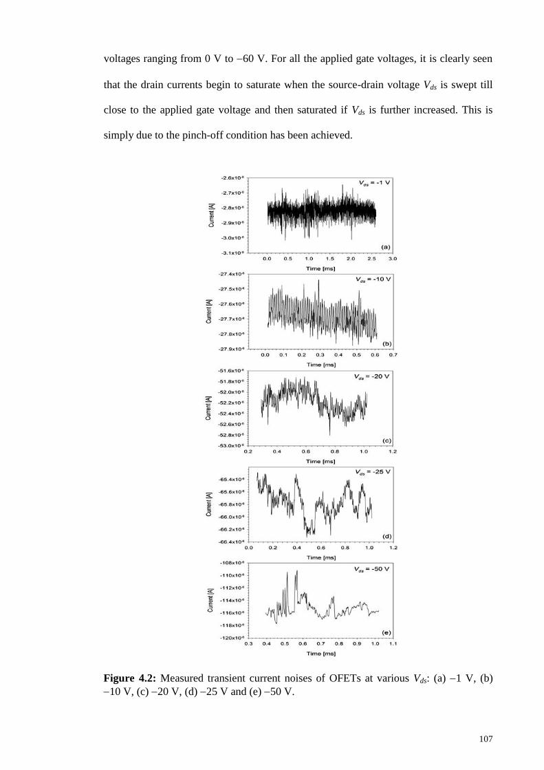
107

voltages ranging from 0 V to 60 V. For all the applied gate voltages, it is clearly seen

that the drain currents begin to saturate when the source-drain voltage Vds is swept till

close to the applied gate voltage and then saturated if Vds is further increased. This is

simply due to the pinch-off condition has been achieved.

Figure 4.2: Measured transient current noises of OFETs at various Vds: (a) 1 V, (b)

10 V, (c) 20 V, (d) 25 V and (e) 50 V.

108

The measured current noises of OFETs at various source-drain voltage Vds ranging

from 1 V to 50 V while having the gate voltage Vg fixed at 60 V are shown in

Figure 4.2(a)-(e). It can be clearly seen that the profile of the current noise is gradually

changing from white noise (rough time series) to 1/f noise and then to Brownian noise

behaviour (smoother time series) as Vds increases. The deviation of behaviour of the

transient current noise at different Vds is also observable through the calculated transient

current noise PSD obtained at high frequency region in which the scaling exponent PS

of the PSD is ranging from around 0.1 (white noise) to 2.0 (Brownian noise) as shown

in Figure 4.3(a)-(e). This observation is further evidenced by the DFA in which the

calculated scaling exponent DFA of the DFA obtained at a short time window is

changing from around 0.5 (white noise) to 1.5 (Brownian noise) as shown in Figure

4.4(a)-(e).

At Vds = 1 V, 1/f noise and shot noise are observed respectively at the low and high

frequency regions of the PSD as shown in Figure 4.3(a). The presence of 1/f noise at the

low frequency region of the PSD is due to the summation of the generation-

recombination noise spectral (Kasap & Capper, 2006). Generation-recombination noise

is due to the random capturing and releasing of charge carries at trap centres. This also

leads to the fluctuation of the number of free charge carriers occurring in the device.

When the device is operated at low voltage (below 2.5 V), free charge carries are

injected from the source contact, undergo trapping and then being released from the trap

centres as they drift across the channel region of the OFET. Hence, each charge carrier

arrives at the drain contact at a purely uncorrelated time. This transport mechanism

causes the occurrence of shot noise in the device. The calculated scaling exponent DFA

of the DFA confirmed that the measured current noise at Vds = 1 V is having the white

noise behaviour as shown in Figure 4.4(a).

109

Figure 4.3: PSDs of transient current noises of OFETs obtained at various Vds: (a) 1 V,

(b) 10 V, (c) 20 V, (d) 25 V and (e) 50 V. The straight line indicates the least-

squares line of the PSD.

110

Figure 4.4: DFA of transient current noises of OFETs obtained at various Vds: (a) 1 V,

(b) 10 V, (c) 20 V, (d) 25 V and (e) 50 V. The straight line indicates the least-

squares line of the DFA.

As Vds increases to 10 V, both the PSD method and DFA indicate that the current

noise presents with 1/f noise at the high frequency region of the PSD (Figure 4.3(b)) and

corresponds to a short time window of the DFA (Figure 4.4(b)). On the other hand,

Brownian noise is detected at low frequency region of the PSD and corresponds to a

111

large time window of DFA. It is also interesting to see that the white noise behaviour of

the current noise is detected by the DFA using a medium time window. When the

device is biased at moderate Vds, free charge carriers are injected from the source

contact into the channel region and all trap centres will be immediately filled first while

the remaining large amount of free charge carries are continuously hopping towards the

drain contact to produce current. Since electric field established at the channel region

extends and covers relatively a larger area as compared to that of the threshold voltage,

thus it contains a larger amount of trap centres that enhances the occurrence of

generation-recombination noise. The summation of the generation-recombination noise

spectral of a larger channel region eventually resulted in 1/f noise that happened at a

very short time period (Kasap & Capper, 2006). After a very short time, all trap centres

have been filled and the remaining free charge carriers are hopping towards the drain

contact in which each hopping is not correlated with each other. Meanwhile, trapped

charge carriers can be released from the trap centres and continue to hop towards the

drain contact. On the other hand, free charge carries can be captured by trap centres

again. Releasing of trapped charge carriers and re-trapping of free charge carriers are

also occurring in an uncorrelated manner. Based on these reasons, the resulted current is

fluctuating randomly like a white noise. In addition, a Brownian noise-like current

fluctuation is detected by both the PSD method and DFA (Figure 4.4(b)). This could be

attributed to the collective effect of hopping, capturing and releasing of charge carriers

over a long time period.

At Vds = 20 V, both the PSD method and DFA indicate that the current noise

presents with 1/f noise for the entire frequency region of the PSD (Figure 4.3(c)) and at

medium time window of DFA (Figure 4.4(c)). This is simply due to the summation of

generation-recombination noise spectra that lead to the 1/f noise when the electric field

extended to cover a larger area of the channel region that contains a relatively huge

112

amount of trap centres as compared to that of the number of trap centres at Vds = 10 V.

Besides that, Brownian noise is detected when the current noise is analysed by DFA

using large time window. This could be attributed to the collective effect of hopping,

capturing and releasing of charge carriers over a long time period as observed at Vds =

10 V. As shown in Figure 4.2(c), it can be seen that the profile of current noise reveals

a slight Brownian noise behaviour that is detectable by DFA. This demonstrates that

DFA is a more sensitive method as compared to PSD method in detecting the

nonstationary properties of the current noise.

At Vds = 25 V, both the PSD method and DFA indicate that the current noise

presents with Brownian noise for the entire frequency region of the PSD (Figure 4.3(d))

and at medium time window of DFA (Figure 4.4(d)). It is interesting to see that charge

carriers are now having an opposite transport dynamics as compared to the transport

dynamics that occurred at lower Vds ( 20 V). This suggests that correlation is induced

between each charge carrier hopping and causes charge carriers hopping like Brownian

particles in the device when the device is operated at high electric field. Besides that, 1/f

noise is observed when the current noise is analysed by DFA method using large time

window in which PSD method is not sensitive enough to reveal this behaviour. The

occurrence of 1/f noise is simply due to the fact that a large amount of trap centres is

provoked by the electrically induced stress on the active material which causes larger

generation-recombination noises. The summation of generation-recombination noise

spectra eventually yields the 1/f noise in the current noise that weakens the existence of

Brownian noise.

Transport dynamics that happened at Vds = 25 V is also reproducible when device

was operated at even higher bias, Vds = 50 V. The scaling exponent DFA of DFA

indicates that charge carriers are hopping like Brownian particles. However, PSD

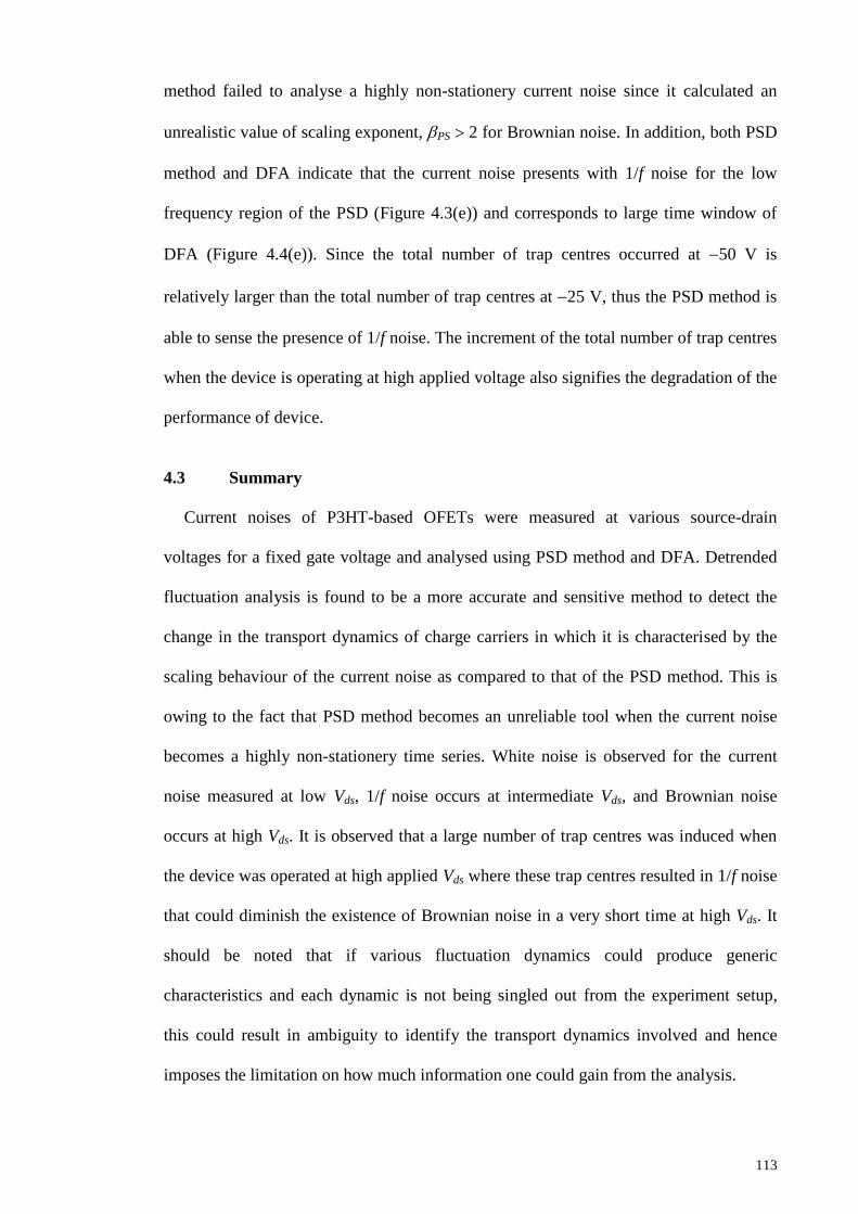
113

method failed to analyse a highly non-stationery current noise since it calculated an

unrealistic value of scaling exponent, PS 2 for Brownian noise. In addition, both PSD

method and DFA indicate that the current noise presents with 1/f noise for the low

frequency region of the PSD (Figure 4.3(e)) and corresponds to large time window of

DFA (Figure 4.4(e)). Since the total number of trap centres occurred at 50 V is

relatively larger than the total number of trap centres at 25 V, thus the PSD method is

able to sense the presence of 1/f noise. The increment of the total number of trap centres

when the device is operating at high applied voltage also signifies the degradation of the

performance of device.

4.3 Summary

Current noises of P3HT-based OFETs were measured at various source-drain

voltages for a fixed gate voltage and analysed using PSD method and DFA. Detrended

fluctuation analysis is found to be a more accurate and sensitive method to detect the

change in the transport dynamics of charge carriers in which it is characterised by the

scaling behaviour of the current noise as compared to that of the PSD method. This is

owing to the fact that PSD method becomes an unreliable tool when the current noise

becomes a highly non-stationery time series. White noise is observed for the current

noise measured at low Vds, 1/f noise occurs at intermediate Vds, and Brownian noise

occurs at high Vds. It is observed that a large number of trap centres was induced when

the device was operated at high applied Vds where these trap centres resulted in 1/f noise

that could diminish the existence of Brownian noise in a very short time at high Vds. It

should be noted that if various fluctuation dynamics could produce generic

characteristics and each dynamic is not being singled out from the experiment setup,

this could result in ambiguity to identify the transport dynamics involved and hence

imposes the limitation on how much information one could gain from the analysis.

114

CHAPTER 5: TRANSPORT STUDY OF RRa-P3HT AND RR-P3HT

Chapter 5 provides the conditions which are needed in the charge transport

simulations for RRa-P3HT at different electric field and RR-P3HT at different light

intensities. The simulated results are then plotted together with the measurement results

extracted from publish works for comparison (Mauer et al., 2010). It is then followed by

the discussions on the anomalous charge transport in these materials and a summary of

the results is provided at the end of this chapter.

5.1 Simulation conditions

A simple one-dimensional structure with equidistance mesh is adopted to represent

the cell of the TOF measurement as depicted in Figure 5.1. Two types of materials are

considered in the simulation so that the simulated results could be compared with the

experiment data that are digitised from Figure 2 and Figure 6 in (Mauer et al., 2010) for

RRa-P3HT and RR-P3HT (~94%), respectively. A light pulse is initially shone on the

top surface of the cell (x = 0) so that free charge carriers are generated just beneath the

surface of the cell and exponentially decaying into the cell according to

0 e a xN x N

, where a is the absorption coefficient, N0 is the photo-generated

charge carrier density and x is the depth beneath the surface of the cell. Charge carriers

are then diffusing and drifting towards the other end of the cell due to the external

electric field.

Figure 5.1: Schematic diagram represents the cell in TOF measurement.

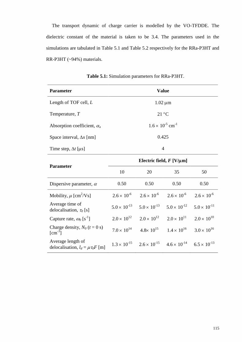
115

The transport dynamic of charge carrier is modelled by the VO-TFDDE. The

dielectric constant of the material is taken to be 3.4. The parameters used in the

simulations are tabulated in Table 5.1 and Table 5.2 respectively for the RRa-P3HT and

RR-P3HT (~94%) materials.

Table 5.1: Simulation parameters for RRa-P3HT.

Parameter Value

Length of TOF cell, L 1.02 m

Temperature, T 21 C

Absorption coefficient, a 1.6 10-5

cm-1

Space interval, x [nm] 0.425

Time step, t [s] 4

Parameter

Electric field, F [V/m]

10 20 35 50

Dispersive parameter, 0.50 0.50 0.50 0.50

Mobility, [cm2/Vs] 2.6 10

-6 2.6 10

-6 2.6 10

-6 2.6 10

-6

Average time of

delocalisation, 0 [s] 5.0 10

-13 5.0 10

-13 5.0 10

-12 5.0 10

-11

Capture rate, 0 [s-1

] 2.0 1012

2.0 1012

2.0 1011

2.0 1010

Charge density, N0 (t = 0 s)

[cm-3

] 7.0 10

14 4.8 10

15 1.4 10

16 3.0 10

16

Average length of

delocalisation, ld = 0F [m] 1.3 10

-15 2.6 10

-15 4.6 10

-14 6.5 10

-13

116

Table 5.2: Simulation parameters for RR-P3HT (~94%).

Parameter Value

Applied bias, V 40 V

Length of TOF cell, L 2 m

Temperature, T 50 C

Absorption coefficient, a 2 10-5

cm-1

Space interval, x [nm] 0.8

Time step, t [s] 0.2

Parameter

Light intensity, I0 [%]

4 10

Dispersive parameter, 0.90 0.99

Mobility, [cm2/Vs] 1.9 10

-5 7.9 10

-5

Average time of

delocalisation, 0 [s] 1.43 10

-13 1.43 10

-12

Capture rate, 0 [s-1

] 7.0 1012

7.0 1011

Charge density, N0 (t = 0 s)

[cm-3

] 1.5 10

17 2.0 10

17

Average length of

delocalisation, ld = 0F [m] 5.4 10

-15 2.3 10

-13

5.2 Results and discussion on transport dynamics of RRa-P3HT and RR-

P3HT

Figure 5.2 shows the transient current curves of RRa-P3HT which were digitised

from Figure 6 in (Mauer et al., 2010) and measured using the TOF measurement at

different electric fields. The transient current curves, represented by different lines in

Figure 5.2, were calculated by the VO-TFDDE and reproduced the experimental results

very well. It can be seen that all the current curves at different electric fields did not

show a plateau or a transition region before they ended with a long-tail on the double-

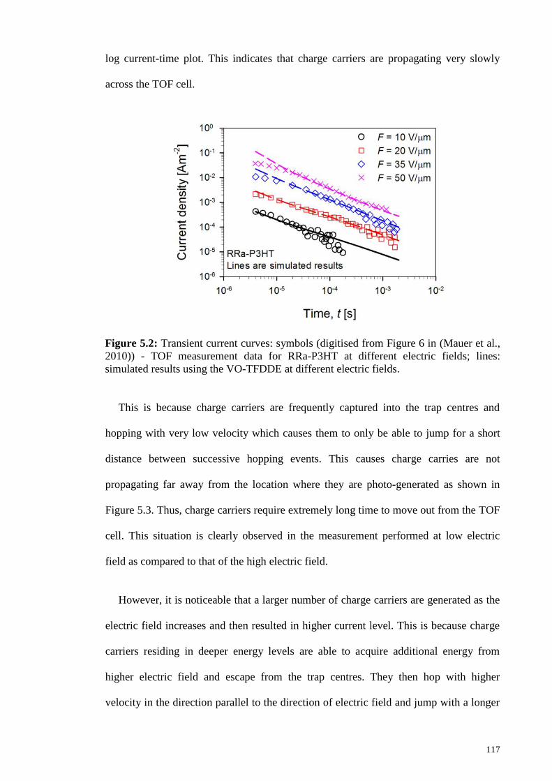
117

log current-time plot. This indicates that charge carriers are propagating very slowly

across the TOF cell.

Figure 5.2: Transient current curves: symbols (digitised from Figure 6 in (Mauer et al.,

2010)) - TOF measurement data for RRa-P3HT at different electric fields; lines:

simulated results using the VO-TFDDE at different electric fields.

This is because charge carriers are frequently captured into the trap centres and

hopping with very low velocity which causes them to only be able to jump for a short

distance between successive hopping events. This causes charge carries are not

propagating far away from the location where they are photo-generated as shown in

Figure 5.3. Thus, charge carriers require extremely long time to move out from the TOF

cell. This situation is clearly observed in the measurement performed at low electric

field as compared to that of the high electric field.

However, it is noticeable that a larger number of charge carriers are generated as the

electric field increases and then resulted in higher current level. This is because charge

carriers residing in deeper energy levels are able to acquire additional energy from

higher electric field and escape from the trap centres. They then hop with higher

velocity in the direction parallel to the direction of electric field and jump with a longer

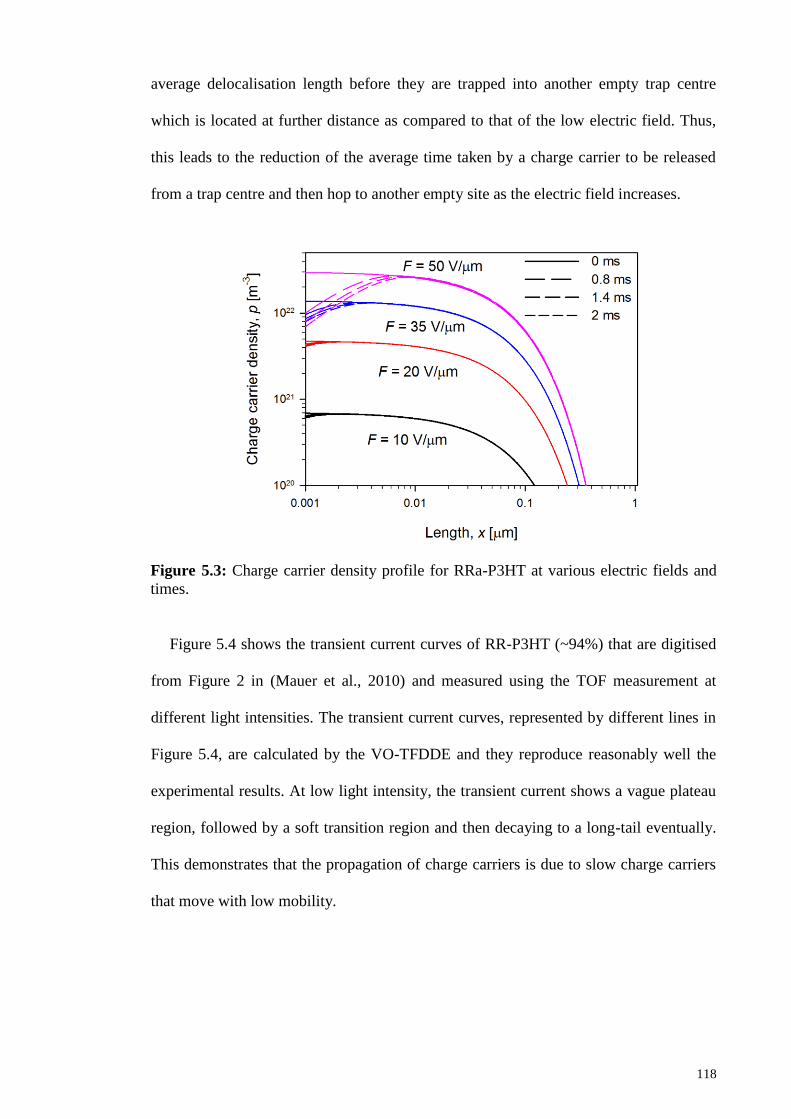
118

average delocalisation length before they are trapped into another empty trap centre

which is located at further distance as compared to that of the low electric field. Thus,

this leads to the reduction of the average time taken by a charge carrier to be released

from a trap centre and then hop to another empty site as the electric field increases.

Figure 5.3: Charge carrier density profile for RRa-P3HT at various electric fields and

times.

Figure 5.4 shows the transient current curves of RR-P3HT (~94%) that are digitised

from Figure 2 in (Mauer et al., 2010) and measured using the TOF measurement at

different light intensities. The transient current curves, represented by different lines in

Figure 5.4, are calculated by the VO-TFDDE and they reproduce reasonably well the

experimental results. At low light intensity, the transient current shows a vague plateau

region, followed by a soft transition region and then decaying to a long-tail eventually.

This demonstrates that the propagation of charge carriers is due to slow charge carriers

that move with low mobility.

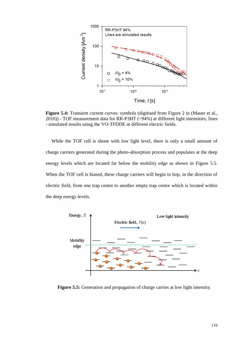
119

Figure 5.4: Transient current curves: symbols (digitised from Figure 2 in (Mauer et al.,

2010)) - TOF measurement data for RR-P3HT (~94%) at different light intensities; lines

- simulated results using the VO-TFDDE at different electric fields.

While the TOF cell is shone with low light level, there is only a small amount of

charge carriers generated during the photo-absorption process and populates at the deep

energy levels which are located far below the mobility edge as shown in Figure 5.5.

When the TOF cell is biased, these charge carriers will begin to hop, in the direction of

electric field, from one trap centre to another empty trap centre which is located within

the deep energy levels.

Figure 5.5: Generation and propagation of charge carries at low light intensity.

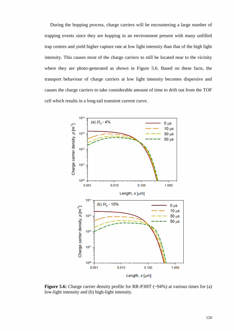
120

During the hopping process, charge carriers will be encountering a large number of

trapping events since they are hopping in an environment present with many unfilled

trap centres and yield higher capture rate at low light intensity than that of the high light

intensity. This causes most of the charge carriers to still be located near to the vicinity

where they are photo-generated as shown in Figure 5.6. Based on these facts, the

transport behaviour of charge carriers at low light intensity becomes dispersive and

causes the charge carriers to take considerable amount of time to drift out from the TOF

cell which results in a long-tail transient current curve.

Figure 5.6: Charge carrier density profile for RR-P3HT (~94%) at various times for (a)

low-light intensity and (b) high-light intensity.

121

In contrast to low light intensity, the transient current measured at higher light

intensity shows a clearer plateau, a transition region and then eventually followed by a

long-tail as shown in Figure 5.4. This indicates that the transport dynamics of charge

carriers is becoming slightly less dispersive as the light intensity increases. At higher

light intensity, a huge number of charge carriers is generated during the photo-

absorption process. These charge carries will be first populating within the deep energy

levels and then the excessive charge carriers will be stacking up to higher energy levels

which are located nearer to the mobility edge as shown in Figure 5.7.

Figure 5.7: Generation and propagation of charge carries at high light intensity.

Charge carrier can now hop at higher velocity from one trap centre to another empty

trap centre which is located close to the mobility edge. They will encounter lesser

capturing event and able to hop at a longer average delocalisation length as compared to

that of the low light intensity. Therefore, the propagation of charge carriers at high light

intensity requires lesser time to leave the TOF cell as shown in Figure 5.6. In view of

the facts that the RR-P3HT has lower capture rate and larger average length of

delocalisation, thus the transport dynamic of charge carriers in RR-P3HT is less

dispersive and much faster than that of the RRa-P3HT.

122

5.3 Summary

The dispersive transport dynamic of charge carriers in organic semiconductors is

modelled using the time-fractional drift-diffusion equation which is approximated using

the finite difference method. Numerical solutions of charge carrier density are obtained

which enables the calculation of transient current density. When electric field is

increased, charge carriers are able to acquire additional energy from the field which

promotes them to be released much easier from the trap centres and then propagating at

higher velocity before leaving the TOF cell that eventually results in higher transient

current. When light intensity is increased, a huge number of charge carriers can be

generated and occupying energy levels close to the mobility edge where charge carriers

will encounter lesser capturing event and hop at a longer average delocalisation length

in each successive hopping. This causes charge carriers to move less depressively for a

short time interval before the occurrence of long-tail behaviour. Besides, the transport

dynamic of charge carriers in RR-P3HT is relatively less dispersive and has higher

mobility than that of the RRa-P3HT since RR-P3HT has lower capturing rate and is less

energy disordered.

123

CHAPTER 6: CONCLUSIONS

Chapter 6 summarises the findings of this work and provides the recommendations

and suggestions for future works.

6.1 Summary

Noise analysis in disordered organic semiconductor devices is frequently overlooked

regardless of the importance of this approach which can be used to explore the transport

dynamics of charge carriers, bulk or interface defects, trap density and structural

properties of disordered organic semiconductors. Besides, the current noise of organic

semiconductor device deviates from the common 1/f noise behaviour which could not

be simply analysed by power spectra method. This work began on the study of transport

dynamics of charge carriers in disordered material by using fractal noise analysis.

Therefore, top-contact and bottom-gate P3HT-based OFETs had been fabricated with

thermal treatment condition. Transient current noises of the OFETs were measured at

various Vds ranging from 0 V to 60 V with respect to a fixed gate voltage of 60 V.

The results from conventional PSD method were compared with the DFA. The latter has

been proven to be a more reliable method for fractal signal analysis particularly in the

presence of nonstationary effects.

Interesting transitions between multiscaling to monoscaling behaviours were

observed in the PSD as well as the DFA plots for different applied Vds. Uncorrelated

white noise characteristics are observed for current noise measured at low Vds,

meanwhile 1/f noise-like scaling behaviours are observed at intermediate Vds. At higher

Vds, the noise characteristics appeared to be close to Brownian-like power-law

behaviour. The scaling characteristics of the transient current noise can be related to the

charge carrier dynamics. It is also found that large numbers of trap centres are induced

when the device is stressed at high applied Vds. The existence of these trap centres

124

would disperse charge carriers, leading to 1/f type noise that could diminish the

presence of Brownian noise in a very short time.

Owing to the fact that anomalous transport has dispersive and non-Gaussian transport

dynamics, thus anomalous transport cannot be adequately described by the standard

drift-diffusion equation which is a framework commonly used to model normal

diffusive transport. Therefore in the second part of this work, the standard drift-

diffusion equation was generalised to TFDDE using the fractional calculus approach to

model the anomalous transport in the RRa-P3HT and RR-P3HT. Physical elucidation of

TFDDE is given by stressing how the influence of the multiple-trapping mechanisms

and disorder in energy lead to the long-tail behaviour in the transient photocurrent

curves.

Time-fractional drift-diffusion equation is solved numerically using finite difference

scheme to obtain the profiles of charge carriers density evolution and hence to

reproduce the corresponding transient photocurrents of RRa-P3HT and RR-P3HT.

Poisson solver is also included in the model to account for the fluctuation of localised

electric field due to the evolution of charge carriers. It is found that charge carriers

acquire additional energy from high electric field that helps them to escape from the trap

centres more easily and then propagating at higher velocity, which yields higher

transient current. Higher concentration of charge carriers can be generated at higher

light intensity and they can occupy energy levels close to the mobility edge, where

charge carriers will encounter smaller capturing rate and hop at a longer length in each

hopping event. Thus, the transport dynamic of charge carriers at high light intensity is

less dispersive than that of the low light intensity. Besides, the transport dynamic of

charge carriers in RR-P3HT is relatively less dispersive and has higher mobility than

that of the RRa-P3HT since RR-P3HT has lower capturing rate and less disorder in

125

energy. It should be noted that the present study employed non-standard method based

on fractal theory and fractional calculus to describe power-law scaling noise spectra and

dispersive charge carrier transport dynamics in disordered organic semiconductors. At

the end of this study, these methods have been proven successfully in describing and

reproducing current noise and charge transport dynamics in disordered organic

semiconductors.

6.2 Recommendation and future works

A large number of grid points and smaller time intervals are needed in order to detect

the rapid change in the transport dynamics of the charge carriers and current density

calculation. This causes a high demand on the memory, computation time as well as

data storage. The recommendations for overcoming these issues could be:

1. adaptive mesh method could be used to replace the equi-distance mesh so that finer

spatial step is used at device region with higher electric field and vice versa.

2. adopt adaptive method on the composite Simpson’s rule to reduce the total number

of grid points used to define the mesh of the TOF cell.

Since molecular recombination is an important process which could cause fluctuation

and reduction in current that leads to performance degradation of device, thus it would

be beneficial to include the effect of molecular recombination in the transport

simulation. In this work, the anomalous transport is modelled by the multiple-trapping

model through the time-fractional drift-diffusion equation. However, the anomalous

transport model could be revised to incorporate the spatial disorder of the material

through the anomalous hopping which is described based on the Lévy flight dynamics.

Thus, anomalous transport produced by the competitiveness between the multiple-

trapping and hopping mechanisms could be modelled together. The suggestions for the

future works are:

126

1. charge carrier generation and recombination mechanism could be incorporated in

the fractional drift-diffusion equation to account for the molecular recombination of

organic semiconductors.

2. the integer order space derivative in the time-fractional drift-diffusion equation

could be rewritten in terms of the fractional space derivative to account for the space

disorder of the organic semiconductors so that the memory effect embedded in the

hopping of charge carrier in space could be modelled by the Lévy flight dynamics.

3. the TFDDE developed in this work is potentially able to be applied to model the

transport dynamics of charge carriers and electric field distribution which is

produced by the SHG measurement.

4. the TFDDE is not only useful to model the subdiffusive transport dynamics of

charge carriers and anomalous current in disordered materials but it could also be

used to model the standard transport dynamics of charge carriers in crystalline

materials.

127

REFERENCES

Agarwal, G. S. (1972). Fluctuation-dissipation theorems for systems in non-thermal

equilibrium and application to laser light. Physics Letters A, 38(2), 93–95.

Assadi, A., Svensson, C., Willander, M., & Inganäs, O. (1988). Field-effect mobility of

poly(3-hexylthiophene). Applied Physics Letters, 53(3), 195–197.

Baeg, K. J., Khim, D. Y., Kim, D. Y., Koo, J. B., You, I. K., Choi, W. S., & Noh, Y. Y.

(2010). High mobility top-gated poly(3-hexylthiophene) field-effect transistors

with high work-function Pt electrodes. Thin Solid Films, 518(14), 4024–4029.

Balakrishnan, V. (1985). Anomalous diffusion in one dimension. Physica A: Statistical

Mechanics and Its Applications, 132(2), 569–580.

Barkai, E. (2001). Fractional Fokker-Planck equation, solution, and application.

Physical Review E, 63(4), 46118.

Barkai, E., Metzler, R., & Klafter, J. (2000). From continuous time random walks to the

fractional Fokker-Planck equation. Physical Review E, 61(1), 132–138.

Barnsley, M. F. (1993). Fractals Everywhere (2nd ed.). Morgan Kaufmann Pub.

Basset, A. B. (1888). A treatise on hydrodynamics with numerous examples. University

of Michigan Library.

Bässler, H. (1993). Charge transport in disordered organic photoconductors a Monte

Carlo simulation study. Physica Status Solidi (B), 175(1), 15–56.

Bazzani, A., Bassi, G., & Turchetti, G. (2003). Diffusion and memory effects for

stochastic processes and fractional Langevin equations. Physica A: Statistical

Mechanics and Its Applications, 324(3), 530–550.

Benten, H., Mori, D., Ohkita, H., & Ito, S. (2016). Recent research progress of polymer

donor/polymer acceptor blend solar cells. Journal of Materials Chemistry A, 4(15),

5340–5365.

Bhatt, M. P., Magurudeniya, H. D., Rainbolt, E. A., Huang, P., Dissanayake, D. S.,

Biewer, M. C., & Stefan, M. C. (2014). Poly(3-Hexylthiophene) nanostructured

materials for organic electronics applications. Journal of Nanoscience and

Nanotechnology, 14(2), 1033–1050.

Bigg, C. (2008). Evident atoms: Visuality in Jean Perrin’s Brownian motion research.

Studies in History and Philosophy of Science Part A, 39(3), 312–322.

Bisquert, J. (2005). Interpretation of a fractional diffusion equation with nonconserved

probability density in terms of experimental systems with trapping or

recombination. Physical Review E, 72(1), 11109.

Borsenberger, P. M., Magin, E. H., Van Auweraer, M. Der, & De Schryver, F. C.

(1993). The role of disorder on charge transport in molecularly doped polymers

128

and related materials. Physica Status Solidi (a), 140(1), 9–47.

Brophy, J. J. (1968). Statistics of 1/f noise. Physical Review, 166(3), 827–831.

Brophy, J. J. (1969). Variance fluctuations in flicker noise and current noise. Journal of

Applied Physics, 40(9), 3551–3553.

Brown, R. (1866). The miscellaneous botanical works of Robert Brown. Volume 1. I.

Geographico-botanical, and, II. Structural and physiological memoirs. London:

The Ray Society.

Burden, L. R., & Faires, J. D. (2011). Numerical Analysis. (M. Julet, Ed.) (9e, Intern

ed.). Canada: Brooks/Cole, Cengage Learning.

Canus, C., Legrand, P., & Véhel, J. L. (2003). FRACLAB: A Fractal Matlab/Scilab

toolbox.

Chandrasekhar, S. (1943). Stochastic problems in physics and astronomy. Reviews of

Modern Physics, 15(1), 1–89.

Chen, H., Guo, Y., Yu, G., Zhao, Y., Zhang, J., Gao, D., Liu, H., & Liu, Y. (2012).

Highly π-extended copolymers with diketopyrrolopyrrole moieties for high-

performance field-effect transistors. Advanced Materials, 24(34), 4618–4622.

Chen, Z., Ivanov, P. C., Hu, K., & Stanley, H. E. (2002). Effect of nonstationarities on

detrended fluctuation analysis. Physical Review. E, Statistical, Nonlinear, and Soft

Matter Physics, 65(4), 41107.

Cheney, W., & Kincaid, D. (2008). Numerical mathematics and computing (6th ed.).

USA: Thomson Brooks/Cole.

Choi, J., Song, H., Kim, N., & Kim, F. S. (2015). Development of n-type polymer

semiconductors for organic field-effect transistors. Semiconductor Science and

Technology, 30(6), 64002.

Coffey, W. T., Kalmykov, Y. P., & Waldron, J. T. (2004). The Langevin equation - with

applications to stochastic problems in physics, chemistry and electrical

engineering (World Scientific series in contemporary chemical physics Vol. 14)

(2nd ed.). World Scientific Publishing Company.

Craciun, N. I. (2011). Electrical characterization of polymeric charge transport layers.

Groningen.

da Silva Jr., M. P., Lyra, M. L., & Vermelho, M. V. D. (2005). Analog study of the first

passage time problem driven by power-law distributed noise. Physica A: Statistical

Mechanics and Its Applications, 348, 85–96.

Dang, M. T., Hirsch, L., & Wantz, G. (2011). P3HT:PCBM, best seller in polymer

photovoltaic research. Advanced Materials, 23(31), 3597–3602.

Das, R. (2017). Printed, Organic & Flexible Electronics Forecasts, Players &

Opportunities 2017-2027. USA.

129

Dong, H., Wang, C., & Hu, W. (2010). High performance organic semiconductors for

field-effect transistors. Chemical Communications, 46(29), 5211–5222.

Dong, J., Yu, P., Arabi, S. A., Wang, J., He, J., & Jiang, C. (2016). Enhanced mobility

in organic field-effect transistors due to semiconductor/dielectric interface control

and very thin single crystal. Nanotechnology, 27(27), 275202.

Dunlap, D. H., & Kenkre, V. M. (1993). Disordered polaron transport: A theoretical

description of the motion of photoinjected charges in molecularly doped polymers.

Chemical Physics, 178(1–3), 67–75.

Ebata, H., Izawa, T., Miyazaki, E., Takimiya, K., Ikeda, M., Kuwabara, H., & Yui, T.

(2007). Highly soluble [1]Benzothieno[3,2-b]benzothiophene (BTBT) derivatives

for high-performance, solution-processed organic field-effect transistors. Journal

of the American Chemical Society, 129(51), 15732–15733.

Ebisawa, F., Kurokawa, T., & Nara, S. (1983). Electrical properties of

polyacetylene/polysiloxane interface. Journal of Applied Physics, 54(6), 3255–

3259.

Einstein, A. (1905). Über die von der molekularkinetischen Theorie der Wärme

geforderte Bewegung von in ruhenden Flüssigkeiten suspendierten Teilchen.

Annalen Der Physik, 17, 549–560.

Falconer, K. (1990). Fractal geometry: Mathematical foundations and applications.

West Sussex, England: John Wiley & Sons Ltd.

Fick, A. (1855). Ueber Diffusion. Annalen Der Physik Und Chemie, 170(1), 59–86.

Fokker, A. D. (1914). Die mittlere Energie rotierender elektrischer Dipole im

Strahlungsfeld. Annalen Der Physik, 348(5), 810–820.

Gajda, J., & Magdziarz, M. (2011). Kramers’ escape problem for fractional Klein-

Kramers equation with tempered α-stable waiting times. Physical Review. E,

Statistical, Nonlinear, and Soft Matter Physics, 84(2), 21137.

Geometric fractals - Chapter 2 fractal dimension. (n.d.). Retrieved December 23, 2016,

from http://fractalfoundation.org/OFC/OFC-index.htm

Günther, A. A., Widmer, J., Kasemann, D., & Leo, K. (2015). Hole mobility in

thermally evaporated pentacene: Morphological and directional dependence.

Applied Physics Letters, 106(23), 233301.

Hartenstein, B., Bässler, H., Heun, S., Borsenberger, P., Van der Auweraer, M., & De

Schryver, F. C. (1995). Charge transport in molecularly doped polymers at low

dopant concentrations: Simulation and experiment. Chemical Physics, 191(1–3),

321–332.

Hasegawa, T., & Takeya, J. (2009). Organic field-effect transistors using single crystals.

Science and Technology of Advanced Materials, 10(2), 24314.

130

Heeger, A. J., Macdiarmid, A. G., & Shirakawa, H. (2002). Alan J. Heeger, Alan G.

MacDiarmid, and Hideki Shirakawa. Macromolecules, 35(4), 1137–1139.

Hilfer, R. (2000a). Applications of fractional calculus in physics. Singapore: World

Scientific Publishing Co. Pie. Ltd.

Hilfer, R. (2000b). Fractional diffusion based on Riemann-Liouville fractional

derivatives. The Journal of Physical Chemistry B, 104(16), 3914–3917.

Ho, S., Liu, S., Chen, Y., & So, F. (2015). Review of recent progress in multilayer

solution-processed organic light-emitting diodes. Journal of Photonics for Energy,

5(1), 57611.

Hofmockel, R., Zschieschang, U., Kraft, U., Rödel, R., Hansen, N. H., Stolte, M.,

Würthner, F., Takimiya, K., Kern, K., Pflaum, J., & Klauk, H. (2013). High-

mobility organic thin-film transistors based on a small-molecule semiconductor

deposited in vacuum and by solution shearing. Organic Electronics, 14(12), 3213–

3221.

Holstein, T. (1959). Studies of polaron motion: Part I. The molecular-crystal model.

Annals of Physics, 8(3), 325–342.

Houssa, M., Vandewalle, N., Nigam, T., Ausloos, M., Mertens, P. W., & Heyns, M. M.

(1998). Analysis of the gate voltage fluctuations in ultra-thin gate oxides after soft

breakdown. In International Electron Devices Meeting 1998. Technical Digest

(Cat. No.98CH36217) (pp. 909–912).

Hu, K., Ivanov, P. C., Chen, Z., Carpena, P., & Stanley, H. E. (2001). Effect of trends

on detrended fluctuation analysis. Physical Review. E, Statistical, Nonlinear, and

Soft Matter Physics, 64(1), 11114.

Hughes, B. D. (1995). Random walks and random environments - Volume 1: Random

walks. Clarendon Press.

Huikuri, H. V, Perkiömäki, J. S., Maestri, R., & Pinna, G. D. (2009). Clinical impact of

evaluation of cardiovascular control by novel methods of heart rate dynamics.

Philosophical Transactions of the Royal Society A: Mathematical, Physical and

Engineering Sciences, 367(1892), 1223–1238.

Huo, Z., Mao, L., Xu, M., & Tan, C. (2003). Low frequency current noise in 2.5 nm

MOSFET and fractal dimension of soft breakdown. Solid-State Electronics, 47(9),

1451–1456.

Ignaccolo, M., Jernajczyk, W., Grigolini, P., & West, B. J. (2010). Dynamics of

electroencephalogram entropy and pitfalls of scaling detection. Physical Review. E,

Statistical, Nonlinear, and Soft Matter Physics, 81(3), 31909.

Irimia-Vladu, M. (2014). “Green” electronics: Biodegradable and biocompatible

materials and devices for sustainable future. Chemical Society Reviews, 43(2),

588–610.

131

Iwamoto, M., Tojima, A., Manaka, T., & Zhong-can, O.-Y. (2003). Compression-shear-

induced tilt azimuthal orientation of amphiphilic monolayers at the air-water

interface: A C∞ → C2v transition in the flow of a two-dimensional hexatic structure.

Physical Review E, 67(4), 41711.

Johanson, R. E., Günes, M., & Kasap, S. O. (2002). Noise in hydrogenated amorphous

silicon. IEE Proceedings - Circuits, Devices and Systems, 149(1), 68–74.

Jurchescu, O. D., Hamadani, B. H., Xiong, H. D., Park, S. K., Subramanian, S.,

Zimmerman, N. M., Anthony, J. E., Jackson, T. N., & Gundlach, D. J. (2008).

Correlation between microstructure, electronic properties and flicker noise in

organic thin film transistors. Applied Physics Letters, 92(13), 132103.

Juška, G., Arlauskas, K., Viliūnas, M., & Kočka, J. (2000). Extraction current

transients: New method of study of charge transport in microcrystalline silicon.

Physical Review Letters, 84(21), 4946–4949.

Kalb, W. L., Mathis, T., Haas, S., Stassen, A. F., & Batlogg, B. (2007). Organic small

molecule field-effect transistors with CytopTM

gate dielectric: Eliminating gate bias

stress effects. Applied Physics Letters, 90(9), 92104.

Kasap, S., & Capper, P. (Eds.). (2006). Springer Handbook of Electronic and Photonic

Materials. Stürtz GmbH, Würzburg, Germany: Springer Science+Business Media,

Inc.

Ke, L., Dolmanan, S., Shen, L., Vijila, C., Chua, S. J., Png, R. Q., Chia, P. J., Chua, L.

L., & Ho, P. K. H. (2008). Low frequency noise analysis on organic thin film

transistors. Journal of Applied Physics, 104(12), 124502.

Ke, L., Zhao, X. Y., Kumar, R. S., & Chua, S. J. (2006). Low-frequency noise

measurement and analysis in organic light-emitting diodes. IEEE Electron Device

Letters, 27(7), 555–557.

King, A. (2016). Fractal - A photographic investigation into fractal forms in science and

nature. Retrieved January 3, 2017, from

http://cargocollective.com/annabelking/Fractal-1

Knauss, D. M., & Huang, T. (2003). ((PS)nPS)m star-shaped polystyrene with star-

shaped branches at the terminal chain ends by convergent living anionic

polymerization. Macromolecules, 36(16), 6036–6042.

Kong, Y. L., Muniandy, S. V., Fakir, M. S., & Sulaiman, K. (2014). Morphological

image interpretation of organic nickel(II) phthalocyanine-tetrasulfonic acid

tetrasodium film using fractal analysis. Applied Surface Science, 301, 363–368.

Kong, Y. L., Muniandy, S. V., Sulaiman, K., & Fakir, M. S. (2017). Random fractal

surface analysis of disordered organic thin films. Thin Solid Films, 623, 147–156.

Kubo, R. (1966). The fluctuation-dissipation theorem. Reports on Progress in Physics,

29(1), 255–284.

132

Lee, J. M., Kim, D. J., Kim, I. Y., Park, K. S., & Kim, S. I. (2004). Nonlinear-analysis

of human sleep EEG using detrended fluctuation analysis. Medical Engineering &

Physics, 26(9), 773–776.

Likhtenshtein, G. I. (2012). Solar energy conversion: Chemical aspects. Wiley-VCH

Verlag GmbH.

Lim, S. C., & Muniandy, S. V. (2002). Self-similar Gaussian processes for modeling

anomalous diffusion. Physical Review. E, Statistical, Nonlinear, and Soft Matter

Physics, 66(2), 21114.

Lin, Y., & Xu, C. (2007). Finite difference/spectral approximations for the time-

fractional diffusion equation. Journal of Computational Physics, 225(2), 1533–

1552.

Loewe, R. S., Khersonsky, S. M., & McCullough, R. D. (1999). A simple method to

prepare head-to-tail coupled, regioregular poly(3-alkylthiophenes) using Grignard

metathesis. Advanced Materials, 11(3), 250–253.

Lutz, E. (2001). Fractional Langevin equation. Physical Review E, 64(5), 51106.

Mainardi, F., & Pironi, P. (1996). The fractional Langevin equation Brownian motion

revisited. Extracta Mathematicae, 11(1), 140–154.

Manaka, T., Lim, E., Tamura, R., & Iwamoto, M. (2005). Modulation in optical second

harmonic generation signal from channel of pentacene field effect transistors

during device operation. Applied Physics Letters, 87(22), 222107.

Manaka, T., Lim, E., Tamura, R., Yamada, D., & Iwamoto, M. (2006). Probing of the

electric field distribution in organic field effect transistor channel by microscopic

second-harmonic generation. Applied Physics Letters, 89(7), 72113.

Mandelbrot, B. B. (1982). The fractal geometry of nature. W. H. Freeman and

Company.

Mandelbrot, B. B., & Van Ness, J. W. (1968). Fractional Brownian motions, fractional

noises and applications. SIAM Review, 10(4), 422–437.

Matsushita, R., Gleria, I., Figueiredo, A., & Da Silva, S. (2007). Are pound and euro the

same currency?, 368(3–4), 173–180.

Mauer, R., Kastler, M., & Laquai, F. (2010). The impact of polymer regioregularity on

charge transport and efficiency of P3HT:PCBM photovoltaic devices. Advanced

Functional Materials, 20(13), 2085–2092.

Mazo, R. M. (2009). Brownian motion: Fluctuations, dynamics, and applications.

(International Series of Monographs on Physics (Book 112), Ed.) (1st ed.). Oxford

University Press.

Mazzio, K. A., & Luscombe, C. K. (2015). The future of organic photovoltaics.

Chemical Society Reviews, 44(1), 78–90.

133

McMullen, C. T. (1998). Hausdorff dimension and conformal dynamics, III:

Computation of dimension. American Journal of Mathematics, 120(4), 691–721.

Metzler, R., Barkai, E., & Klafter, J. (1999). Deriving fractional Fokker-Planck

equations from a generalised master equation. Europhysics Letters, 46(4), 431–

436.

Metzler, R., & Klafter, J. (2000a). Boundary value problems for fractional diffusion

equations. Physica A: Statistical Mechanics and Its Applications, 278(1), 107–125.

Metzler, R., & Klafter, J. (2000b). Subdiffusive transport close to thermal equilibrium:

From the Langevin equation to fractional diffusion. Physical Review E, 61(6),

6308–6311.

Metzler, R., & Klafter, J. (2000c). The random walk’s guide to anomalous diffusion: A

fractional dynamics approach. Physics Reports, 339(1), 1–77.

Metzler, R., & Klafter, J. (2004). The restaurant at the end of the random walk: Recent

developments in the description of anomalous transport by fractional dynamics.

Journal of Physics A: Mathematical and General, 37(31), R161–R208.

Meyer, M., & Stiedl, O. (2003). Self-affine fractal variability of human heartbeat

interval dynamics in health and disease. European Journal of Applied Physiology,

90(3), 305–316.

Milichko, V. A., Shalin, A. S., Mukhin, I. S., Kovrov, A. E., Krasilin, A. A.,

Vinogradov, A. V., Belov, P. A., & Simovski, C. R. (2016). Solar photovoltaics:

Current state and trends. Physics-Uspekhi, 59(8), 727–772.

Miller, A., & Abrahams, E. (1960). Impurity conduction at low concentrations. Physical

Review, 120(3), 745–755.

Minemawari, H., Yamada, T., Matsui, H., Tsutsumi, J., Haas, S., Chiba, R., Kumai, R.,

& Hasegawa, T. (2011). Inkjet printing of single-crystal films. Nature, 475(7356),

364–367.

Mori, T. (2008). Molecular materials for organic field-effect transistors. Journal of

Physics: Condensed Matter, 20(18), 184010.

Mott, N. F., & Twose, W. D. (1961). The theory of impurity conduction. Advances in

Physics, 10(38), 107–163.

Mozer, A. J., Sariciftci, N. S., Lutsen, L., Vanderzande, D., Österbacka, R., Westerling,

M., & Juška, G. (2005). Charge transport and recombination in bulk heterojunction

solar cells studied by the photoinduced charge extraction in linearly increasing

voltage technique. Applied Physics Letters, 86(11), 112104.

Murio, D. A. (2008a). Implicit finite difference approximation for time fractional

diffusion equations. Computers & Mathematics with Applications, 56(4), 1138–

1145.

134

Murio, D. A. (2008b). Time fractional IHCP with Caputo fractional derivatives.

Computers & Mathematics with Applications, 56(9), 2371–2381.

Myny, K., van Veenendaal, E., Gelinck, G. H., Genoe, J., Dehaene, W., & Heremans, P.

(2012). An 8-bit, 40-instructions-per-second organic microprocessor on plastic foil.

IEEE Journal of Solid-State Circuits, 47(1), 284–291.

Nawaz, A., Meruvia, M. S., Tarange, D. L., Gopinathan, S. P., Kumar, A., Kumar, A.,

Bhunia, H., Pal, A. J., & Hümmelgen, I. A. (2016). High mobility organic field-

effect transistors based on defect-free regioregular poly(3-hexylthiophene-2,5-

diyl). Organic Electronics, 38, 89–96.

Nelkin, M., & Harrison, A. K. (1982). Random-walk model for the saturation of 1/f

noise amplitudes. Physical Review B, 26(12), 6696–6705.

Øksendal, B. (2003). Stochastic differential equations. Berlin, Heidelberg: Springer

Berlin Heidelberg.

Pénarier, A., Jarrix, S. G., Delseny, C., Pascal, F., Vildeuil, J. C., Valenza, M., &

Rigaud, D. (2002). Low-frequency noise in III–V high-speed devices. IEE

Proceedings - Circuits, Devices and Systems, 149(1), 59–67.

Peng, C. K., Buldyrev, S. V., Havlin, S., Simons, M., Stanley, H. E., & Goldberger, A.

L. (1994). Mosaic organization of DNA nucleotides. Physical Review E, 49(2),

1685–1689.

Peng, C. K., Havlin, S., Stanley, H. E., & Goldberger, A. L. (1995). Quantification of

scaling exponents and crossover phenomena in nonstationary heartbeat time series.

Chaos (Woodbury, N.Y.), 5(1), 82–87.

Penzel, T., Kantelhardt, J. W., Grote, L., Peter, J. H., & Bunde, A. (2003). Comparison

of detrended fluctuation analysis and spectral analysis for heart rate variability in

sleep and sleep apnea. IEEE Transactions on Biomedical Engineering, 50(10),

1143–1151.

Perrin, J., Macleod, A. R., & Soddy, F. (1910). Brownian movement and molecular

reality. London: Taylor and Francis.

Pivrikas, A., Juska, G., Arlauskas, K., Scharber, M., Mozer, A., Sariciftci, N. S., Stubb,

H., & Österbacka, R. (2005). Charge carrier transport and recombination in bulk-

heterojunction solar-cells. In Z. H. Kafafi & P. A. Lane (Eds.) (p. 59380N).

Podlubny, I. (Ed.). (1998). Fractional differential equations: An introduction to

fractional derivatives, fractional differential equations, to methods of their solution

and some of their applications. USA: Academic Press.

Risken, H., & Frank, T. (1996). The Fokker-Planck equation: Methods of solution and

applications (Springer series in synergetics, book 18). (H. Haken, Ed.) (2nd ed.).

Berlin Heidelberg: Springer-Verlag.

Sapoval, B., Rosso, M., & Gouyet, J. F. (1985). The fractal nature of a diffusion front

and the relation to percolation. Journal de Physique Lettres, 46(4), 149–156.

135

Scalas, E., Gorenflo, R., & Mainardi, F. (2000). Fractional calculus and continuous-time

finance. Physica A: Statistical Mechanics and Its Applications, 284(1–4), 376–384.

Scher, H., & Montroll, E. W. (1975). Anomalous transit-time dispersion in amorphous

solids. Physical Review B, 12(6), 2455–2477.

Schmidt, R., Oh, J. H., Sun, Y. Sen, Deppisch, M., Krause, A. M., Radacki, K.,

Braunschweig, H., Könemann, M., Erk, P., Bao, Z., & Würthner, F. (2009). High-

performance air-stable n-channel organic thin film transistors based on halogenated

perylene bisimide semiconductors. Journal of the American Chemical Society,

131(17), 6215–6228.

Schneider, W. R., & Wyss, W. (1989). Fractional diffusion and wave equations. Journal

of Mathematical Physics, 30(1), 134–144.

Sekine, C., Tsubata, Y., Yamada, T., Kitano, M., & Doi, S. (2014). Recent progress of

high performance polymer OLED and OPV materials for organic printed

electronics. Science and Technology of Advanced Materials, 15(3), 34203.

Shiau, Y. H. (2011). Understanding as well as characterization of erratic interspike

dynamics in semiconductor devices, 151(2), 135–138.

Shirota, Y., & Kageyama, H. (2007). Charge carrier transporting molecular materials

and their applications in devices. Chemical Reviews, 107(4), 953–1010.

Shukla, D., Nelson, S. F., Freeman, D. C., Rajeswaran, M., Ahearn, W. G., Meyer, D.

M., & Carey, J. T. (2008). Thin-film morphology control in naphthalene-diimide-

based semiconductors: High mobility n-type semiconductor for organic thin-film

transistors. Chemistry of Materials, 20(24), 7486–7491.

Sibatov, R. T., & Uchaikin, V. V. (2007). Fractional differential kinetics of charge

transport in unordered semiconductors. Semiconductors, 41(3), 335–340.

Sibatov, R. T., & Uchaikin, V. V. (2009). Fractional differential approach to dispersive

transport in semiconductors. Physics-Uspekhi, 52(10), 1019–1043.

Silva, L. B. M., Vermelho, M. V. D., Lyra, M. L., & Viswanathan, G. M. (2009).

Multifractal detrended fluctuation analysis of analog random multiplicative

processes. Chaos, Solitons & Fractals, 41(5), 2806–2811.

Sirringhaus, H. (2014). 25th

anniversary article: Organic field-effect transistors: The

path beyond amorphous silicon. Advanced Materials, 26(9), 1319–1335.

Sokolov, I. M., Klafter, J., & Blumen, A. (2002). Fractional kinetics. Physics Today,

55(11), 48–54.

Sousa, E. (2012). How to approximate the fractional derivative of order 1 < α ≤ 2.

International Journal Bifurcation and Chaos, 22(4), 1250075.

Stafström, S. (2010). Electron localization and the transition from adiabatic to

nonadiabatic charge transport in organic conductors. Chemical Society Reviews,

39(7), 2484–2499.

136

Stanley, H. E. (1984). Application of fractal concepts to polymer statistics and to

anomalous transport in randomly porous media. Journal of Statistical Physics,

36(5), 843–860.

Sun, H., Chen, W., Li, C., & Chen, Y. (2012). Finite difference schemes for variable-

order time fractional diffusion eqaution. International Journal of Bifurcation and

Chaos, 22(4), 1250085.

Takamatsu, A., Takaba, E., & Takizawa, G. (2009). Environment-dependent

morphology in plasmodium of true slime mold Physarum polycephalum and a

network growth model. Journal of Theoretical Biology, 256(1), 29–44.

Tanase, C., Meijer, E. J., Blom, P. W. M., & De Leeuw, D. M. (2003). Unification of

the hole transport in polymeric field-effect transistors and light-emitting diodes.

Physical Review Letters, 91(21), 216601.

Terje, A. S., & Reynolds, J. (Eds.). (2006). Handbook of conducting polymers -

conjugated polymers: Processing and applications (3rd ed.). U.S.A.: CRC Press.

Tessler, N., Preezant, Y., Rappaport, N., & Roichman, Y. (2009). Charge transport in

disordered organic materials and its relevance to thin-film devices: A tutorial

review. Advanced Materials, 21(27), 2741–2761.

Tiwari, S., & Greenham, N. C. (2009). Charge mobility measurement techniques in

organic semiconductors. Optical and Quantum Electronics, 41(2), 69–89.

Tsumura, A., Koezuka, H., & Ando, T. (1986). Macromolecular electronic device:

Field-effect transistor with a polythiophene thin film. Applied Physics Letters,

49(18), 1210–1212.

Turner, M. J., Blackledge, J. M., & Andrews, P. R. (1998). Fractal geometry in digital

imaging. San Diego, USA: Academic Press.

Uchaikin, V. V., & Sibatov, R. T. (2008). Fractional theory for transport in disordered

semiconductors. Communications in Nonlinear Science and Numerical Simulation,

13(4), 715–727.

Uchaikin, V. V., & Sibatov, R. T. (2013). Fractional kinetics in solids: Anomalous

charge transport in semiconductors, dielectrics and nanosystems. Singapore:

World Scientific Publishing Co. Pte. Ltd.

von Smoluchowski, M. (2010). Versuch einer mathematischen Theorie der

Koagulationskinetik kolloider Lösungen. Zeitschrift Fuer Physikalische Chemie,

92, 129–168.

Wang, L., He, X., & Chen, Y. (2011). Diffusion-limited hyperbranched polymers with

substitution effect. The Journal of Chemical Physics, 134(10), 104901.

Wiener, N. (1923). Differential-space. Journal of Mathematics and Physics, 2(1–4),

131–174.

137

Witten, T. A., & Sander, L. M. (1983). Diffusion-limited aggregation. Physical Review

B, 27(9), 5686–5697.

Wool, R. P., & Long, J. M. (1993). Fractal structure of polymer interfaces.

Macromolecules, 26(19), 5227–5239.

Wyss, W. (1986). The fractional diffusion equation. Journal of Mathematical Physics,

27(11), 2782–2785.

Xu, Y., Minari, T., Tsukagoshi, K., Gwoziecki, R., Coppard, R., Balestra, F.,

Chroboczek, J. A., & Ghibaudo, G. (2010). Extraction of low-frequency noise in

contact resistance of organic field-effect transistors. Applied Physics Letters, 97(3),

33503.

Yang, Q., Liu, F., & Turner, I. (2009). Computationally efficient numerical methods for

time- and space-fractional Fokker–Planck equations. Physica Scripta, T136, 14026.

Zhao, Y., Guo, Y., & Liu, Y. (2013). 25th

anniversary article: Recent advances in n-type

and ambipolar organic field-effect transistors. Advanced Materials, 25(38), 5372–

5391.

Zwanzig, R. (2001). Nonequilibrium statistical mechanics. New York, USA: Oxford

University Press.

138

LIST OF PUBLICATIONS AND PAPERS PRESENTED

Journal papers

1. Choo, K. Y., Muniandy, S. V., Chua, C. L. and Woon, K. L. (2012). Scaling

behaviors of transient noise current in organic field-effect transistors. Organic

Electronics, 13(8), 1370-1376.

139

2. Choo, K. Y., Muniandy, S. V., Woon, K. L., Gan, M. T. and Ong, D. S. (2017).

Modeling anomalous charge carrier transport in disordered organic semiconductors

using the fractional drift-diffusion equation. Organic Electronics, 41, 157-165.

140

Proceeding/Conference papers

1. Muniandy, S. V., Woon, K. L. and Choo, K. Y. (2011). Anomalous charge transport

in disordered organic semiconductors. AIP Conf. Proc. Malaysia Annual Physics

Conference, 1328, 38-42.

141

2. Choo, K. Y. and Muniandy, S. V. (2015). Fractional dispersive transport in

inhomogeneous organic semiconductors. Int. J. Mod. Phys.: Conf., 36, 1560008 (16

pages).

142

Conference/Symposium Presentations


Dispersive charge transport study in periodic structures of crystalline-amorphous

hybrid organic materials. 8th

Conference of Asian Consortium on Computational

Materials Science (ACCMS-8), National Taiwan University of Science and

Technology (NTUST), Taipei, Taiwan on June 16-18. 2015.


Fractional dynamics of dispersive transport in organic semiconductors.

University of Malaya-Academia Sinica Research Symposium, University of

Malaya, Kuala Lumpur, Malaysia on 18 November 2015.

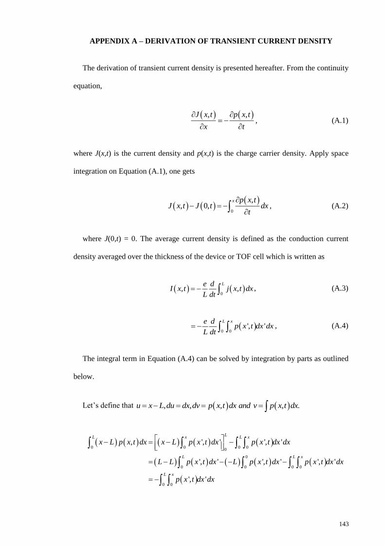
143

APPENDIX A – DERIVATION OF TRANSIENT CURRENT DENSITY

The derivation of transient current density is presented hereafter. From the continuity

equation,

, ,J x t p x t

x t

, (A.1)

where J(x,t) is the current density and p(x,t) is the charge carrier density. Apply space

integration on Equation (A.1), one gets

0

,, 0,

x p x tJ x t J t dx

t

, (A.2)

where J(0,t) = 0. The average current density is defined as the conduction current

density averaged over the thickness of the device or TOF cell which is written as

0

, ,Le d

I x t j x t dxL dt

, (A.3)

0 0

', 'L xe d

p x t dx dxL dt

, (A.4)

The integral term in Equation (A.4) can be solved by integration by parts as outlined

below.

Let’s define that , , , , .u x L du dx dv p x t dx and v p x t dx

0 0 0 00

0

0 0 0 0

0 0

, ', ' ', '

', ' ', ' ', '

', '

LL x L x

L L x

L x

x L p x t dx x L p x t dx p x t dx dx

L L p x t dx L p x t dx p x t dx dx

p x t dx dx

144

Thus, the average transient current density can also be written as

0

, ,Le d

I x t x L p x t dxL dt

. (A.5)

145

APPENDIX B – PROGRAMMING CODE DEVELOPED FOR ANOMALOUS

CHARGE TRANSPORT

The following code was developed by the author of the thesis and it is fully belong to

the author. No partial of the code is allowed to be reused or reproduced in any meant

without the permission of the author. The pseudo code of the programming is given

below.

(a) Device and material parameters

The device and material parameters needed for the programme are listed in the Table

5.1 and Table 5.2 respectively for RRa-P3HT and RR-P3HT (~94%).

inTPDE_v001o_P3HT.txt

Fractional order value: sa

Select variable order alfa (YES=1): opsa

Use non-even time step dt (YES=1): opdt

Temperature: temp

Applied bias: Va

Total no. spatial step: NX

Spatial step: dx

Total no. time step: TL

Time step: dt

Initial concentration: cimp

Background concentration: cint

Static relative permittivity: eps

Mobility-electron: mue

Lifetime (equilibrium): tau0e

Capture rate: wratee

Mean trap energy: en0

Absorption coefficient: abscoe

(b) Main programme – TFDE_vs001o

The main programme starts the simulation by sequentially calling to the subroutines

defined in the main programme TFDE_vs001o.

Program begin

call readin ! Input device and material parameters

call paras ! Preprocess input parameters

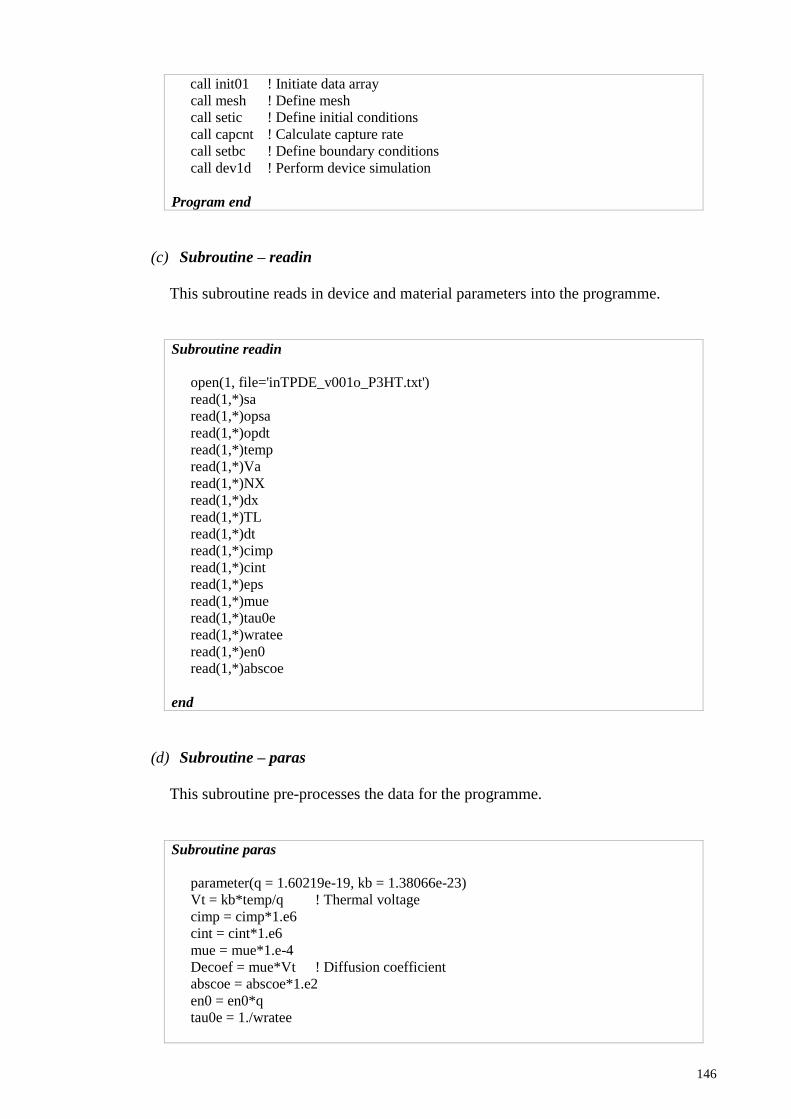
146

call init01 ! Initiate data array

call mesh ! Define mesh

call setic ! Define initial conditions

call capcnt ! Calculate capture rate

call setbc ! Define boundary conditions

call dev1d ! Perform device simulation

Program end

(c) Subroutine – readin

This subroutine reads in device and material parameters into the programme.

Subroutine readin

open(1, file='inTPDE_v001o_P3HT.txt')

read(1,*)sa

read(1,*)opsa

read(1,*)opdt

read(1,*)temp

read(1,*)Va

read(1,*)NX

read(1,*)dx

read(1,*)TL

read(1,*)dt

read(1,*)cimp

read(1,*)cint

read(1,*)eps

read(1,*)mue

read(1,*)tau0e

read(1,*)wratee

read(1,*)en0

read(1,*)abscoe

end

(d) Subroutine – paras

This subroutine pre-processes the data for the programme.

Subroutine paras

parameter(q = 1.60219e-19, kb = 1.38066e-23)

Vt = kb*temp/q ! Thermal voltage

cimp = cimp*1.e6

cint = cint*1.e6

mue = mue*1.e-4

Decoef = mue*Vt ! Diffusion coefficient

abscoe = abscoe*1.e2

en0 = en0*q

tau0e = 1./wratee

147

end

(e) Subroutine – init01

This subroutine initiates the data arrays needed for the programme.

Subroutine init01

NX1 = NX + 1

TL1 = TL + 1

c

do 10, i = 1,NX1

ix = i

xp(ix) = 0.000000

10 continue

c

do 20, n = 1,TL1

it = n

tn(it) = 0.000000

20 continue

c

do 40, n = 1,TL1

it = n

do 40, i = 1,NX1

ix = i

sole(ix,it) = 0.000000

Vdxe(ix,it) = 0.000000

vex(ix,it) = 0.000000

fx(ix,it) = 0.000000

40 continue

end

(f) Subroutine – mesh

This subroutine sets up the mesh space and time interval for the programme.

Subroutine mesh

do 10, i = 1,NX1

ix = i

xp(ix) = float(i-1)*dx

10 continue

c

Ldev = xp(NX1)

c

if(opdt==1)then

TLR1 = 250

TLR2 = 250

TLR3 = 250

TLR4 = 250

rngT1 = 1.e-6

148

rngT2 = 250.e-6

rngT3 = 500.e-6

rngT4 = 750.e-6

rngT5 = 1.e-3

dt1 = (rngT2-rngT1)/TLR1




c

do 20, n = 1,TL1

it = n

if(it.le.TLR1)then

tn(it) = float(it-1)*dt1

elseif(it.le.(TLR1+TLR2))then

tn(it) = float(it-TLR1)*dt2 + tn(TLR1)

elseif(it.le.(TLR1+TLR2+TLR3))then

tn(it) = float(it-(TLR1+TLR2))*dt3 + tn(TLR1+TLR2)

elseif(it.le.(TLR1+TLR2+TLR3+TLR4+1))then

tn(it) = float(it-(TLR1+TLR2+TLR3))*dt4+tn(TLR1+TLR2+TLR3)

end if

20 continue

else

do 25, n = 1,TL1

it = n

tn(it) = float(n-1)*dt

25 continue

end if

c

tmax = tn(TL1)

end

(g) Subroutine – setic

This subroutine defines the initial conditions for the TFDDE.

Subroutine setic

it = 1

do 10, i = 1,NX1

ix = i

if(xp(ix).le.Ldev)then

sole(ix,it) = cimp*exp(-abscoe*xp(ix))

else

sole(ix,it) = 0.000000

end if

10 continue

end

149

(h) Subroutine – capcnt

This subroutine calculates the capture coefficient.

Subroutine capcnt

parameter(pi = 3.141592654, q = 1.60219e-19, kb = 1.38066e-23)

do 10, ix=1,NX1

do 20, it=1,TL1

aftem = fsa(xp(ix),tn(it),opsa)

alfae(ix,it) = aftem

if(aftem.le.0.)then

cape(ix,it) = wratee

elseif(aftem.ge.0.99999)then

cape(ix,it) = 0.000000

else

cape(ix,it) = wratee* (sin(pi*aftem)/(pi*aftem))**(1./aftem)

end if

20 continue

10 continue

end

(i) Subroutine – setbc

This subroutine sets up the boundary conditions for charge carrier density and

electric potential.

Subroutine setbc

ib1 = 1

ib2 = NX1

c

do 30, n = 1,TL1

it = n

sole(ib1,it) = 0.0000000 ! carrier density, u(1,t)

sole(ib2,it) = 0.0000000 ! carrier density, u(NX1,t)

Vdxe(ib1,it) = Va

Vdxe(ib2,it) = 0.0000000

30 continue

c

do 45, i = 1,NX1-2

ix = i

call poisoe(ix,0)

45 continue

c

call pfebs(0)

call newfx(0)

end

150

(j) Subroutine – dev1d

This subroutine performs the device simulation up to the predetermined total

simulation time.

Subroutine dev1d

do 10, n = 1,TL1-1

do 20, i = 1,NX1-2

call tfpde(i,n)

20 continue

c

call mfebs(n)

call Itxe(n)

c

do 40, i = 1,NX1-2

call poisoe(i,n)

40 continue

c

call pfebs(n)

call newfx(n)

c

10 continue

end

(k) Subroutine – tfpde(i,n)

This subroutine calculates the coefficients of the system of linear equations

representing the time-fractional drift-diffusion equation and assigns them into matrix

forms.

Subroutine tfpde(inx,int)

it = int

ix = inx + 1

sumsol = 0.0000000

sdt = tn(it+1)-tn(it)

c---diffusion term

diffe1 = -(Decoef*fgma(2.-alfae(ix,it+1))*sdt**alfae(ix,it+1))/(dx**2)

diffe2 = (Decoef*fgma(2.-alfae(ix,it+1))*sdt**alfae(ix,it+1))/(dx**2)

diffe3 = -(Decoef*fgma(2.-alfae(ix,it+1))*sdt**alfae(ix,it+1))/(dx**2)

c---drift term

drfe1 = -(vex(ix,it)*fgma(2.-alfae(ix,it+1))*sdt**alfae(ix,it+1))/(2.*dx)

drfe3 = (vex(ix,it)*fgma(2.-alfae(ix,it+1))*sdt**alfae(ix,it+1))/(2.*dx)

drfe2 = ((vex(ix+1,it)-vex(ix-1,it))*fgma(2.-

alfae(ix,it+1))*sdt**alfae(ix,it+1))/(2.*dx)

c---calculate 0c

rcef1 = tau0e*cape(ix,it+1)**alfae(ix,it+1)

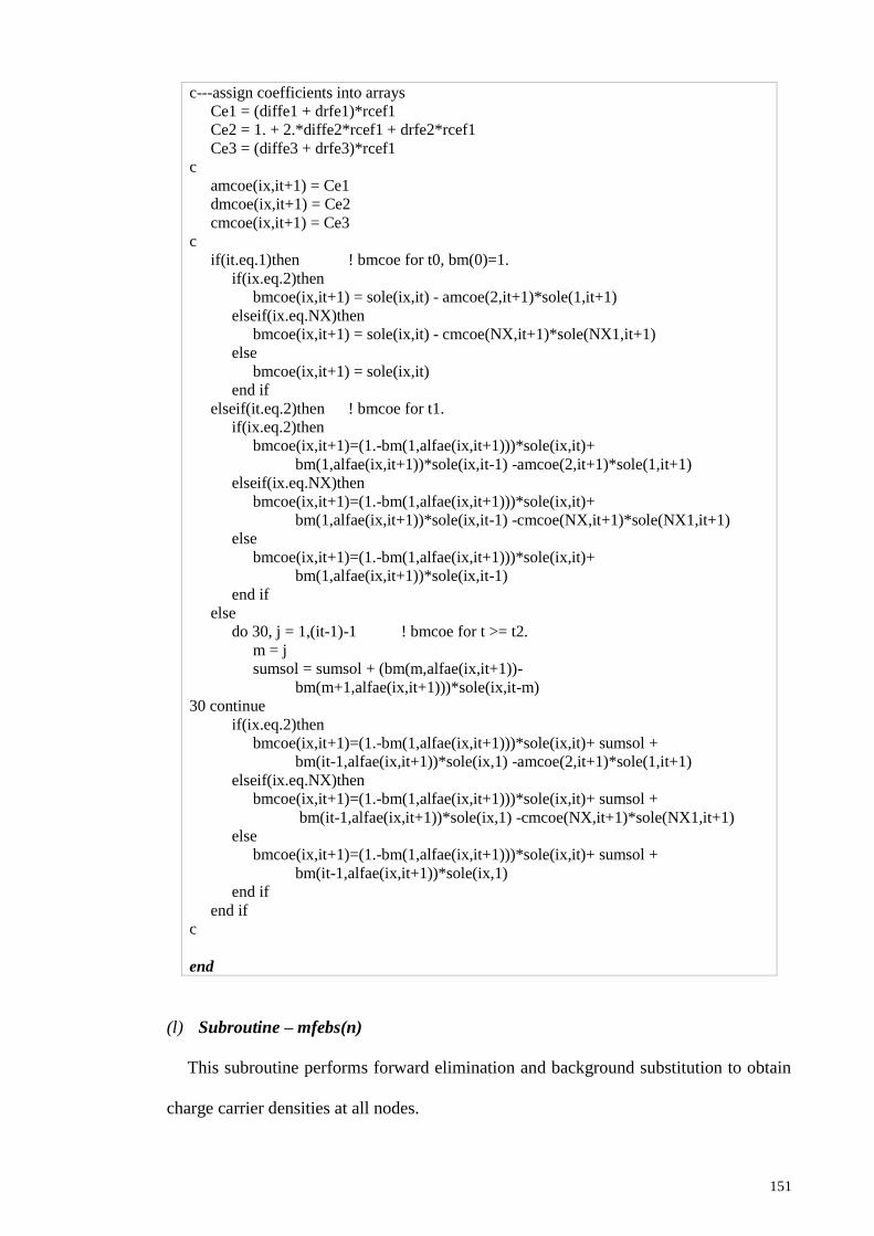
151

c---assign coefficients into arrays

Ce1 = (diffe1 + drfe1)*rcef1

Ce2 = 1. + 2.*diffe2*rcef1 + drfe2*rcef1

Ce3 = (diffe3 + drfe3)*rcef1

c

amcoe(ix,it+1) = Ce1

dmcoe(ix,it+1) = Ce2

cmcoe(ix,it+1) = Ce3

c

if(it.eq.1)then ! bmcoe for t0, bm(0)=1.

if(ix.eq.2)then

bmcoe(ix,it+1) = sole(ix,it) - amcoe(2,it+1)*sole(1,it+1)

elseif(ix.eq.NX)then

bmcoe(ix,it+1) = sole(ix,it) - cmcoe(NX,it+1)*sole(NX1,it+1)

else

bmcoe(ix,it+1) = sole(ix,it)

end if

elseif(it.eq.2)then ! bmcoe for t1.

if(ix.eq.2)then

bmcoe(ix,it+1)=(1.-bm(1,alfae(ix,it+1)))*sole(ix,it)+

bm(1,alfae(ix,it+1))*sole(ix,it-1) -amcoe(2,it+1)*sole(1,it+1)



bm(1,alfae(ix,it+1))*sole(ix,it-1) -cmcoe(NX,it+1)*sole(NX1,it+1)

else


bm(1,alfae(ix,it+1))*sole(ix,it-1)

end if

else

do 30, j = 1,(it-1)-1 ! bmcoe for t >= t2.

m = j

sumsol = sumsol + (bm(m,alfae(ix,it+1))-

bm(m+1,alfae(ix,it+1)))*sole(ix,it-m)

30 continue

if(ix.eq.2)then

bmcoe(ix,it+1)=(1.-bm(1,alfae(ix,it+1)))*sole(ix,it)+ sumsol +

bm(it-1,alfae(ix,it+1))*sole(ix,1) -amcoe(2,it+1)*sole(1,it+1)



bm(it-1,alfae(ix,it+1))*sole(ix,1) -cmcoe(NX,it+1)*sole(NX1,it+1)

else


bm(it-1,alfae(ix,it+1))*sole(ix,1)

end if

end if

c

end

(l) Subroutine – mfebs(n)

This subroutine performs forward elimination and background substitution to obtain

charge carrier densities at all nodes.

152

Subroutine mfebs(int)

it = int

c---forward elimination

do 100, i = 1,NX1-3

ix = i + 2

mfac = amcoe(ix,it+1)/dmcoe(ix-1,it+1)

dcoe = dmcoe(ix,it+1) - mfac*cmcoe(ix-1,it+1)

bcoe = bmcoe(ix,it+1) - mfac*bmcoe(ix-1,it+1)

dmcoe(ix,it+1) = dcoe

bmcoe(ix,it+1) = bcoe

100 continue

c---backward substitution

sole(NX,it+1) = bmcoe(NX,it+1)/dmcoe(NX,it+1)

c

do 200, i = NX1-2,2,-1

ix = i

sole(ix,it+1) = (bmcoe(ix,it+1)-cmcoe(ix,it+1)*sole(ix+1,it+1))/dmcoe(ix,it+1)

200 continue

end

(m) Subroutine – Itxe(n)

This subroutine calculates the average total current density.

Subroutine Itxe(int)

parameter(q = 1.60219e-19)

it = int

sI01 = 0.0000000

sI02 = 0.0000000

sdt = tn(it+1)-tn(it)

atem = q/sdt

btem = dx/3.

c---lower and upper bounds

sILB = (xp(1)/Ldev-1.)*(sole(1,it+1)-sole(1,it))

sIUB = (xp(NX1)/Ldev-1.)*(sole(NX1,it+1)-sole(NX1,it))

c---terms with factor 4

do 10, i = 1,floor(NX/2.)

ix = 2*i

sI01 = sI01 + 4.*(xp(ix)/Ldev-1.)*(sole(ix,it+1)-sole(ix,it))

10 continue

c---terms with factor 2

do 20, i = 1,ceiling((NX/2.)-1.)

ix = 2*i + 1

sI02 = sI02 + 2.*(xp(ix)/Ldev-1.)*(sole(ix,it+1)-sole(ix,it))

20 continue

c---average total current density

Iext(it+1) = atem*btem*(sILB+sIUB+sI01+sI02)

end

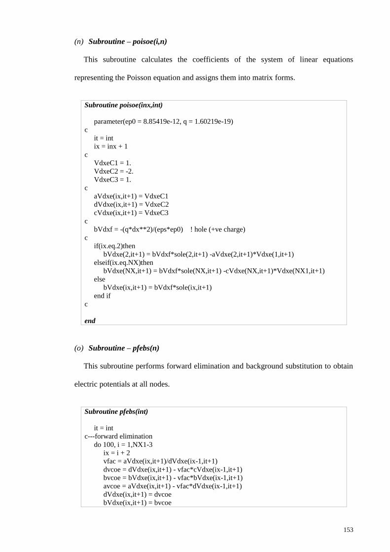
153

(n) Subroutine – poisoe(i,n)

This subroutine calculates the coefficients of the system of linear equations

representing the Poisson equation and assigns them into matrix forms.

Subroutine poisoe(inx,int)

parameter(ep0 = 8.85419e-12, q = 1.60219e-19)

c

it = int

ix = inx + 1

c

VdxeC1 = 1.

VdxeC2 = -2.

VdxeC3 = 1.

c

aVdxe(ix,it+1) = VdxeC1

dVdxe(ix,it+1) = VdxeC2

cVdxe(ix,it+1) = VdxeC3

c

bVdxf = -(q*dx**2)/(eps*ep0) ! hole (+ve charge)

c

if(ix.eq.2)then

bVdxe(2,it+1) = bVdxf*sole(2,it+1) -aVdxe(2,it+1)*Vdxe(1,it+1)


bVdxe(NX,it+1) = bVdxf*sole(NX,it+1) -cVdxe(NX,it+1)*Vdxe(NX1,it+1)

else

bVdxe(ix,it+1) = bVdxf*sole(ix,it+1)

end if

c

end

(o) Subroutine – pfebs(n)

This subroutine performs forward elimination and background substitution to obtain

electric potentials at all nodes.

Subroutine pfebs(int)

it = int

c---forward elimination

do 100, i = 1,NX1-3

ix = i + 2

vfac = aVdxe(ix,it+1)/dVdxe(ix-1,it+1)

dvcoe = dVdxe(ix,it+1) - vfac*cVdxe(ix-1,it+1)

bvcoe = bVdxe(ix,it+1) - vfac*bVdxe(ix-1,it+1)

avcoe = aVdxe(ix,it+1) - vfac*dVdxe(ix-1,it+1)

dVdxe(ix,it+1) = dvcoe

bVdxe(ix,it+1) = bvcoe

154

aVdxe(ix,it+1) = avcoe

100 continue

c---backward substitution

Vdxe(NX,it+1) = bVdxe(NX,it+1)/dVdxe(NX,it+1)

c

do 200, i = NX1-2,2,-1

ix = i

Vdxe(ix,it+1) = (bVdxe(ix,it+1)-cVdxe(ix,it+1)*Vdxe(ix+1,it+1))/dVdxe(ix,it+1)

200 continue

end

(p) Subroutine – newfx(n)

This subroutines calculate new electric field and velocity based on the updated

charge carrier density profile.

Subroutine newfx(int)

it = int

c

do 100, i = 1,NX1-2

ix = i + 1

fx(ix,it+1) = -(Vdxe(ix+1,it+1)-Vdxe(ix-1,it+1))/(2.*dx)

100 continue

c

fx(1,it+1) = -(Vdxe(2,it+1) - Vdxe(1,it+1))/dx

fx(NX1,it+1) = -(Vdxe(NX1,it+1) - Vdxe(NX,it+1))/dx

c

do 110, j = 1,NX1

ix = j

vex(ix,it+1) = mue*fx(ix,it+1) ! Velocity in x-direction.

110 continue

end

(q) function – bm(m,alfae(ix,it+1))

This function calculates the , 1m k

ib value given in Equation (3.19).

function bm(m,sabm)

bm = float(m+1)**(1.-sabm) - float(m)**(1.-sabm)

end

(r) function – fsa(xp(ix),tn(it),opsa)

This function calculates the fractional order or material disordered value.

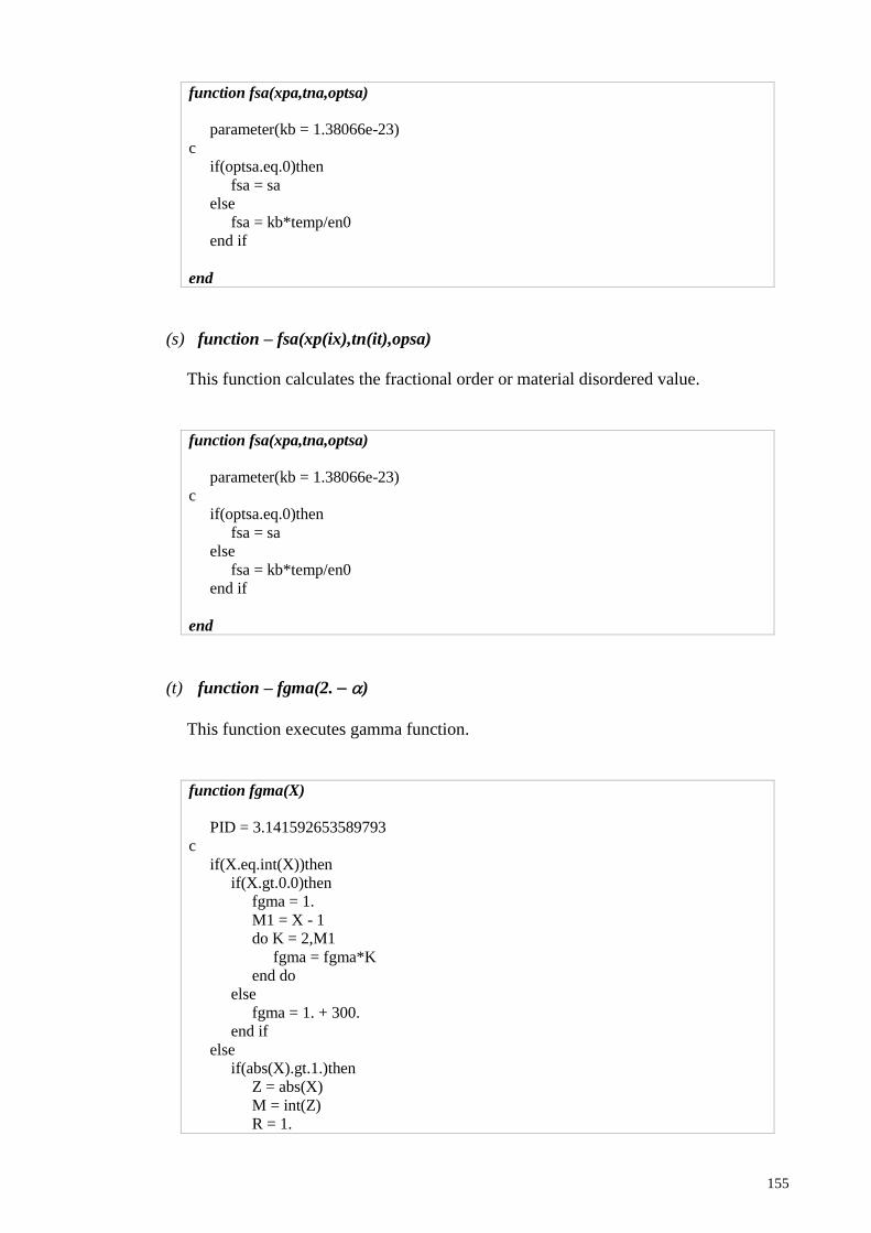
155

function fsa(xpa,tna,optsa)

parameter(kb = 1.38066e-23)

c

if(optsa.eq.0)then

fsa = sa

else

fsa = kb*temp/en0

end if

end

(s) function – fsa(xp(ix),tn(it),opsa)

This function calculates the fractional order or material disordered value.

function fsa(xpa,tna,optsa)

parameter(kb = 1.38066e-23)

c

if(optsa.eq.0)then

fsa = sa

else

fsa = kb*temp/en0

end if

end

(t) function – fgma(2. )

This function executes gamma function.

function fgma(X)

PID = 3.141592653589793

c

if(X.eq.int(X))then

if(X.gt.0.0)then

fgma = 1.

M1 = X - 1

do K = 2,M1

fgma = fgma*K

end do

else

fgma = 1. + 300.

end if

else

if(abs(X).gt.1.)then

Z = abs(X)

M = int(Z)

R = 1.

156

do K = 1,M

R = R*(Z-K)

end do

Z = Z - M

else

Z = X

end if

c

DATA G/1.0D0,0.5772156649015329D0, -0.6558780715202538D0,

-0.420026350340952D-1, 0.1665386113822915D0,-.421977345555443D-1,

-.96219715278770D-2, .72189432466630D-2, -.11651675918591D-2,

-.2152416741149D-3,.1280502823882D-3, -.201348547807D-4,

- .12504934821D-5, .11330272320D-5, -.2056338417D-6, .61160950D-8,

.50020075D-8, -.11812746D-8,.1043427D-9, .77823D-11, -.36968D-11,

.51D-12, -.206D-13, -.54D-14, .14D-14, .1D-15/

c

GR = G(26)

c

do K = 25,1,-1

GR = GR*Z + G(K)

end do

c

fgma=1./(GR*Z)

if(abs(X).gt.1.)then

fgma = fgma*R

if(X.lt.0.) fgma = -PID/(X*fgma*sin(PID*X))

end if

end if

c

end

157

APPENDIX C - STABILITY TEST AND CONVERGENCE ANALYSIS

(a) Stability test

Let’s define that ,

k k k

j a j jz p p , where , ,k

a j j kp p x t and k

jp represent the actual

and approximate solutions at (xj, tk), and k

jz at point xj = jx (j = 0, 1,..., Nx) can be

expanded by using a Fourier series as, (Sun et al., 2012),

2k i qx L

k

q

z x q e

, (C.1)

where the time index k = 1, 2,..., Nt, L = Nxx represents the total length and

2

0

1 Lk i qx L

k q z x e dxL

. (C.2)

The round-off error equations for the implicit scheme of Equation (3.42) and Equation

(3.43) are respectively written as

1 1 1 1 1 1 1 1 1

, , 1 , , , , 1

11, 1 , 1 1, 1 , 1 0

1

1 2

1 , 1.

k k k k k k k k k

D j v j j D j F j j D j v j j


j j j j j j j

m

C C z C C z C C z

b z b b z b z k

. (C.3)

1 1 1 1 1 1 1 1 1 0,1 0

, , 1 , , , , 11 2 , 0.D j v j j D j F j j D j v j j j jC C z C C z C C z b z k (C.4)

One can assume that

' 2k i qx L k t i j

j k kz e e e , (C.5)

and ' k t

k ke and 2 q x L . Thus, Equation (C.3) and Equation (C.4) are

rewritten as

158

1 11 1 1 1 1 1

, , 1 , , 1 , , 1

11, 1 , 1 1, 1 , 1

0

1

1 2

1 , 1.

i j i jk k k k i j k k

D j v j k D j F j k D j v j k

kk i j m k m k i j k k i j

j k j j k m j

m

C C e C C e C C e

b e b b e b e k

(C.6)

1 11 1 1 1 1 1

, , 1 , , 1 , , 1

0,1

0

1 2

, 0

i j i ji j

D j v j D j F j D j v j

i j

j

C C e C C e C C e

b e k

(C.7)

Equations (C.6) and (C.7) can be rearranged and simplified to obtain k+1 and 1 as

1

1, 1 , 1 1, 1 , 1

0

11

1 1 2 1

, , ,

1

, 1.

1 4 sin 2 sin2

kk m k m k k k

j k j j k m j

mk

k k k

F j D j v j

b b b b

k

C C i C

(C.8)

0,1

0

11 1 2 1

, , ,

, 0.

1 4 sin 2 sin2

j

F j D j v j

bk

C C i C

(C.9)

Since 0,1 1jb , one obtains that 1 0 as the denominators of Equation (C.8) and

Equation (C.9) are greater than unity. One can also write 0m for m = 2, 3,..., k,

then Equation (C.8) and Equation (C.9) respectively become

1

1, 1 , 1 1, 1 , 1

11 0

1 1 2 1

, , ,

1

, 1.

1 4 sin 2 sin2

kk m k m k k k

j j j j

mk

k k k

F j D j v j

b b b b

k

C C i C

(C.10)

01

1 1 2 1

, , ,

, 0.

1 4 sin 2 sin2

F j D j v j

k

C C i C

(C.11)

159

It is demonstrated in (Lin & Xu, 2007) that 1

1, 1 , 1 1, 1 , 1

1

1 1k

k m k m k k k

j j j j

m

b b b b

,

thus Equation (C.10) reduced to

01 0

1 1 2 1

, , ,

, 1.

1 4 sin 2 sin2

kk k k

F j D j v j

k

C C i C

(C.12)

Thus, it could be concluded that the implicit difference scheme is unconditional

stable as being proved by Equation (C.12).

(b) Convergence Analysis

Let’s define that ,

k k k

j a j jz p p , where , ,k

a j j kp p x t and k

jp represent the actual

and approximate solutions at (xj, tk) for j = 0, 1, 2,..., Nx and k = 0, 1, 2,..., Nt. The error

equations for the implicit scheme of Equation (3.42) and Equation (3.43), with 0 0jz ,

are written as (Sun et al., 2012),

1 1 1 1 1 1 1 1 1

, , 1 , , , , 1

11, 1 , 1 1, 1 1

1

1 2

1 , 1.

k k k k k k k k k

D j v j j D j F j j D j v j j

kk k m k m k k m k

j j j j j j

m

C C z C C z C C z

b z b b z k

(C.13)

where

1 1 1 1 1 1 1 1 1 1

, , , 1 , , , , , , 1

11, 1 , 1 1, 1 , 1 0

, , ,

1

1 2

1 .

k k k k k k k k k k

j D j v j a j D j F j a j D j v j a j


j a j j j a j j a j

m

C C p C C p C C p

b p b b p b p

(C.14)

1 1 1 1 1 1 1 1 1 1

, , 1 , , , , 11 2 , 0,D j v j j D j F j j D j v j j jC C z C C z C C z k (C.15)

where

160

1 1 1 1 1 1 1 1 1 1

, , , 1 , , , , , , 1

0,1 0

,

1 2

.

j D j v j a j D j F j a j D j v j a j

j a j

C C p C C p C C p

b p

(C.16)

Equation (3.18), Equation (3.15) and Equation (3.14) can be written as

1 1

1

, 11 0

1 11 , 1 1, 11

0

, ,,

,,2

k kj j

kj

k kj k j j

j k km k m kkj j j k mj

m

p x t b p x tp x t t

C tb b p x tt

(C.17)

221 1 1 1 1 1

2 22

, , 2 , ,,

j k j k j k j kp x t p x t p x t p x tC x

x x

(C.18)

and

1 1 1 1 1

3

, , ,.

2

j k j k j kp x t p x t p x tC x

x x

(C.19)

By using Equation (C.17) to Equation (C.19), Equation (C.14) can be written as

1

1

1

1 1 1

2

1 1

21

1

1 1

21

1 2 3

, ,

,2

, ,

kj

kj k

j

k k kj j j

j k j k

k

j k

j

j k j k

p x t p x t

t xt

F x t p x tx

C t C t x C t x

(C.20)

which gives

1 1 1211 ,

k k kj j jk

j C t t x t x

(C.21)

where C1, C2, C3 and C are constants. Thus, the implicit scheme is convergent as

1 1 1211

, 1, 0,1,2,..., -1.

k k kj j jk

j tk k

j

Cz t t x t x k N

b

(C.22)

MODELLING OF ANOMALOUS CHARGE CARRIERS … · TRANSPORT IN DISORDERED ORGANIC SEMICONDUCTORS CHOO...

Documents

Transcript of MODELLING OF ANOMALOUS CHARGE CARRIERS … · TRANSPORT IN DISORDERED ORGANIC SEMICONDUCTORS CHOO...