Modelling Epidemic Spread using Cellular Automata - Computer

Modelling Epidemic

Spread using Cellular

Automata

Shih Ching Fu

This report is submitted as partial fulfilment

of the requirements for the Honours Programme of the

Department of Computer Science and Software Engineering,

The University of Western Australia,

2002

Abstract

Most existing epidemic models make simplifying assumptions about the underly-ing environmental conditions they are trying to emulate. Of particular interest isthe assumption of a homogeneous world where not only are all the hosts identical,they are uniformly distributed over the landscape. Making such an assumptionlimits the realism of these models. To improve realism we should incorporatespatial heterogeneity. Cellular automata (CA) implicitly model space in theirstructure making them an attractive prospect for incorporating spatial factorsinto epidemic modelling. Using CA to model epidemics is not a new concept,however previous models have usually focused on one or two epidemic spreadparameters in order to isolate and analyse their impact. As far as creating a pre-dictive tool is concerned, we require a model that will take into account all themajor epidemic spread factors and produce a reasonable depiction of the future.

Not only can a CA model trivially implement many of the parameters foundin existing differential equation models, but they provide a useful tool for thegraphical visualisation of an epidemic’s spread. The model proposed in thisdissertation is far from complete and requires extensive quantitative data for val-idation purposes. Initial results suggest that through the use of simple localizedinteraction rules, an accurate overall epidemic behaviour can be emulated.

Keywords: Cellular automata, epidemic, simulation.CR Categories: F.1.1, I.6.8

ii

Acknowledgements

First and foremost I would like to thank my supervisor Professor George Milne.His interest and enthusiasm in my project was motivation for me to work thatextra bit harder. I appreciate that he supervised a number of other Honoursstudents this year as well. I would also like to thank Dr Gareth Lee for proofreading my thesis in Professor Milne’s absence.

I would also like to thank our Head of Department, Professor Robyn Owens.Not only did her Scientific Communication unit teach me a lot about writing andpresenting, but the support she has provided the Honours students this year wasinvaluable.

Thanks must also go out every member of the Honours Class of 2002. Weare a close knit group and their company made this year all the more enjoyable,even at the expense of a little productivity!

Finally of course I would like to thank my family for their support and en-couragement through out this year.

iii

Contents

Abstract ii

Acknowledgements iii

1 Introduction 1

2 Basic Viral and Epidemic Theory 3

2.1 What is a virus? . . . . . . . . . . . . . . . . . . . . . . . . . . . 3

2.1.1 Definition . . . . . . . . . . . . . . . . . . . . . . . . . . . 3

2.1.2 Infection life-cycle . . . . . . . . . . . . . . . . . . . . . . . 3

2.1.3 Transmission . . . . . . . . . . . . . . . . . . . . . . . . . 5

2.1.4 Mutation . . . . . . . . . . . . . . . . . . . . . . . . . . . 5

2.2 What is an epidemic? . . . . . . . . . . . . . . . . . . . . . . . . . 6

2.2.1 Definition . . . . . . . . . . . . . . . . . . . . . . . . . . . 6

2.2.2 Transmission probability . . . . . . . . . . . . . . . . . . . 6

2.2.3 Basic reproductive number, R0 . . . . . . . . . . . . . . . 7

2.2.4 Virulence . . . . . . . . . . . . . . . . . . . . . . . . . . . 7

2.2.5 Periodicity . . . . . . . . . . . . . . . . . . . . . . . . . . . 7

3 Cellular Automata 8

3.1 The Cell . . . . . . . . . . . . . . . . . . . . . . . . . . . . . . . . 8

3.2 Update rules . . . . . . . . . . . . . . . . . . . . . . . . . . . . . . 9

3.3 Interaction neighbourhoods . . . . . . . . . . . . . . . . . . . . . 9

4 Review of the Literature 10

4.1 Parameters that influence epidemic spread . . . . . . . . . . . . . 10

4.2 Differential equation models . . . . . . . . . . . . . . . . . . . . . 11

4.3 MFT approximation . . . . . . . . . . . . . . . . . . . . . . . . . 12

iv

4.4 Spatial models: CA . . . . . . . . . . . . . . . . . . . . . . . . . . 13

4.4.1 Variable population size . . . . . . . . . . . . . . . . . . . 14

4.4.2 Uneven population density . . . . . . . . . . . . . . . . . . 14

4.4.3 Variable susceptibility . . . . . . . . . . . . . . . . . . . . 15

4.4.4 Incubation and latency time . . . . . . . . . . . . . . . . . 15

4.4.5 Conclusion . . . . . . . . . . . . . . . . . . . . . . . . . . . 15

5 My Epidemic Model 16

5.1 Cell Definition . . . . . . . . . . . . . . . . . . . . . . . . . . . . . 16

5.2 World Definition . . . . . . . . . . . . . . . . . . . . . . . . . . . 17

5.3 Adjustable Simulation Parameters . . . . . . . . . . . . . . . . . . 17

5.3.1 Neighbourhood radius . . . . . . . . . . . . . . . . . . . . 17

5.3.2 Motion probability . . . . . . . . . . . . . . . . . . . . . . 18

5.3.3 Immigration rate . . . . . . . . . . . . . . . . . . . . . . . 18

5.3.4 Birth rate . . . . . . . . . . . . . . . . . . . . . . . . . . . 19

5.3.5 Natural death rate . . . . . . . . . . . . . . . . . . . . . . 19

5.3.6 Virus morbidity . . . . . . . . . . . . . . . . . . . . . . . . 19

5.3.7 Vectored infection rate . . . . . . . . . . . . . . . . . . . . 20

5.3.8 Contact infection probability . . . . . . . . . . . . . . . . . 20

5.3.9 Spontaneous infection probability . . . . . . . . . . . . . . 20

5.3.10 Recovery rate . . . . . . . . . . . . . . . . . . . . . . . . . 21

5.3.11 Re–susceptible rate . . . . . . . . . . . . . . . . . . . . . . 21

5.4 Cell update algorithm . . . . . . . . . . . . . . . . . . . . . . . . 21

5.4.1 Movement phase . . . . . . . . . . . . . . . . . . . . . . . 21

5.4.2 Infection and recover phase . . . . . . . . . . . . . . . . . 22

6 Control Scenario 23

6.1 World setup . . . . . . . . . . . . . . . . . . . . . . . . . . . . . . 23

6.2 Parameter settings . . . . . . . . . . . . . . . . . . . . . . . . . . 23

6.3 Results . . . . . . . . . . . . . . . . . . . . . . . . . . . . . . . . . 24

6.4 Discussion . . . . . . . . . . . . . . . . . . . . . . . . . . . . . . . 25

v

7 Viral Parameter Experiments 27

7.1 Residual immunity . . . . . . . . . . . . . . . . . . . . . . . . . . 27

7.1.1 World setup . . . . . . . . . . . . . . . . . . . . . . . . . . 27

7.1.2 Parameter settings . . . . . . . . . . . . . . . . . . . . . . 28

7.1.3 Results . . . . . . . . . . . . . . . . . . . . . . . . . . . . . 28

7.1.4 Discussion . . . . . . . . . . . . . . . . . . . . . . . . . . . 30

7.2 High virulence . . . . . . . . . . . . . . . . . . . . . . . . . . . . . 30

7.2.1 World setup . . . . . . . . . . . . . . . . . . . . . . . . . . 30


7.2.3 Results . . . . . . . . . . . . . . . . . . . . . . . . . . . . . 31

7.2.4 Discussion . . . . . . . . . . . . . . . . . . . . . . . . . . . 33

8 Spatial Experiments 35

8.1 Varied population density . . . . . . . . . . . . . . . . . . . . . . 35

8.1.1 World setup . . . . . . . . . . . . . . . . . . . . . . . . . . 35


8.1.3 Results . . . . . . . . . . . . . . . . . . . . . . . . . . . . . 38

8.1.4 Discussion . . . . . . . . . . . . . . . . . . . . . . . . . . . 39

8.2 Host immigration . . . . . . . . . . . . . . . . . . . . . . . . . . . 40

8.2.1 World setup . . . . . . . . . . . . . . . . . . . . . . . . . . 40


8.2.3 Results . . . . . . . . . . . . . . . . . . . . . . . . . . . . . 40

8.2.4 Discussion . . . . . . . . . . . . . . . . . . . . . . . . . . . 43

8.3 Corridors of spread . . . . . . . . . . . . . . . . . . . . . . . . . . 43

8.3.1 World setup . . . . . . . . . . . . . . . . . . . . . . . . . . 43


8.3.3 Results . . . . . . . . . . . . . . . . . . . . . . . . . . . . . 44

8.3.4 Discussion . . . . . . . . . . . . . . . . . . . . . . . . . . . 45

8.4 Barriers to spread . . . . . . . . . . . . . . . . . . . . . . . . . . . 45

8.4.1 World setup . . . . . . . . . . . . . . . . . . . . . . . . . . 45


vi

8.4.3 Results . . . . . . . . . . . . . . . . . . . . . . . . . . . . . 47

8.4.4 Discussion . . . . . . . . . . . . . . . . . . . . . . . . . . . 49

9 Conclusion 50

10 Future work 52

10.1 Model calibration . . . . . . . . . . . . . . . . . . . . . . . . . . . 52

10.2 Different cell types . . . . . . . . . . . . . . . . . . . . . . . . . . 53

10.3 Other tools . . . . . . . . . . . . . . . . . . . . . . . . . . . . . . 53

A SimDemic 57

A.1 Habitable.java . . . . . . . . . . . . . . . . . . . . . . . . . . . 57

A.2 World.java . . . . . . . . . . . . . . . . . . . . . . . . . . . . . . 58

A.3 Cell.java . . . . . . . . . . . . . . . . . . . . . . . . . . . . . . . 59

A.4 The GUI . . . . . . . . . . . . . . . . . . . . . . . . . . . . . . . . 59

B Original Honours Proposal 61

vii

List of Tables

4.1 Various epidemic models and the realism parameters they implement. 13

6.1 Epidemic spread parameter values for the control scenario. . . . . 24

7.1 Parameter values for the residual immunity experiment . . . . . . 28

7.2 Parameter values for the virus morbidity experiment . . . . . . . 31

8.1 Parameter values for the population density experiment . . . . . . 37

8.2 Parameter values for the host immigration experiment . . . . . . 41

viii

List of Figures

2.1 Infection life-cycle . . . . . . . . . . . . . . . . . . . . . . . . . . . 4

3.1 A general CA cell state transition . . . . . . . . . . . . . . . . . . 8

3.2 Commonly used interaction neighbourhoods . . . . . . . . . . . . 9

6.1 Control scenario: ratio of infectives to total population over time . 25

6.2 Control scenario: total population over time . . . . . . . . . . . . 26

7.1 Residual immunity: ratio of infectives to total population over time 29

7.2 Residual immunity: total population over time . . . . . . . . . . . 29

7.3 High virulence: infective ratio over time . . . . . . . . . . . . . . 32

7.4 High virulence: total population over time . . . . . . . . . . . . . 32

7.5 High virulence: effects of immunity . . . . . . . . . . . . . . . . . 34

8.1 High to low population density gradient . . . . . . . . . . . . . . 36

8.2 Low to high population density gradient . . . . . . . . . . . . . . 36

8.3 Decreasing population density: ratio of infectives . . . . . . . . . 38

8.4 Increasing population density: ratio of infectives . . . . . . . . . . 39

8.5 Population dynamics of the closed population experiment . . . . . 42

8.6 Population dynamics of the open population experiment . . . . . 42

8.7 Corridors of spread . . . . . . . . . . . . . . . . . . . . . . . . . . 44

8.8 Corridors of spread: lag map . . . . . . . . . . . . . . . . . . . . . 46

8.9 Barriers to spread . . . . . . . . . . . . . . . . . . . . . . . . . . . 47

8.10 Barriers to spread: lag map . . . . . . . . . . . . . . . . . . . . . 48

A.1 A screen capture of the SimDemic application. . . . . . . . . . . . 60

ix

CHAPTER 1

Introduction

Public health issues are seeing greater visibility in the media; a particular concernis viral spread through populated areas. Decreased worker productivity as aresult of viral illness costs industry millions of dollars every year [4]. With recentvirus epidemics such as foot and mouth disease in the United Kingdom andthe threat of using viruses such as smallpox as biological warfare agents, themonitoring of outbreaks is gaining importance for governments and public healthofficials. It therefore becomes desirable to predict patterns of viral infectionunder certain environments. It is hoped that the modelling of a phenomenonsuch as virus spread will help us understand, predict, and ultimately control thatphenomenon’s behaviour.

The majority of existing epidemic models utilize differential equations and donot take into account spatial factors such as population density. These modelsassume populations are closed and well mixed; that is, host numbers are constantand individuals are free to move wherever they wish. When trying to devise morerealistic models it makes sense to incorporate spatial parameters that reflect theheterogeneous environment found in nature. An alternative to using deterministicdifferential equations is to use a two-dimensional cellular automaton that reliesupon stochastic parameters.

The focus of this dissertation is to analyse how we can use a two-dimensionalCA to model the spread of a viral epidemic. Of particular interest is the mannerin which CA discretize space and I hope to show that spatial heterogeneity can beeasily incorporated into a CA epidemic model. The hypothesis is that the overallbehaviour of an epidemic can be produced from the summation of localized hostinteractions. To demonstrate this hypothesis, it will be necessary to devise anepidemic model and the show that this model can replicate the results of existingnon-CA models, as well as taking space into account.

Before beginning the modelling process, modellers must decide what levelof detail their models will examine. This is an important decision because toomuch detail will produce a cluttered and unworkable model, whereas too little

1

detail provides no useful information. Chapter 4 outlines some of the existingapproaches that have been adopted for epidemic modelling and looks at whichepidemic spread factors, or level of detail, they have chosen to implement. Aftera brief overview of basic epidemic theory and cellular automata in Chapters 2and 3, I will describe the elements of my new composite epidemic model and theepidemic spread parameters I have chosen to implement. Chapters 6, 7 and 8describe the experiments I have conducted to analyse the suitability of CA toepidemic modelling, which also serve to partially validate the epidemic model Idevised as a part of this project.

2

CHAPTER 2

Basic Viral and Epidemic Theory

In contrast with medicine, epidemiology studies the health of entire populationsrather than just the individual. This chapter outlines some of the concepts as-sociated with what is traditionally a statistical field and defines some of theterms you are likely to encounter in epidemiological articles and publications.Although epidemics can stem from any infectious disease, I will focus solely onviral epidemics.

2.1 What is a virus?

2.1.1 Definition

Andrewes [3] describes viruses as “on the borderline between life and death”.Under a microscope a virus resembles little more than a lifeless geometric crystal.However, when a virus penetrates the cell of a living organism it is able to rapidlyreplicate itself.

A virus comprises two parts: some genetic material and a protective proteincoating. After a virus has penetrated a living cell it rewrites the cell’s DNAand transforms it into an organism that produces hundreds or even thousandsof copies of itself. When these virus copies leave the infected cell they are onceagain lifeless until they penetrate another cell. Disease arises from cell damagecaused by the genetic rewriting procedure.

2.1.2 Infection life-cycle

The aim of a virus entering a living cell is to replicate itself, however as the hostacquires antibodies to fight the infection the virus will need to find another host.Consequently, after being infected, an individual usually becomes infectious aswell as diseased. A diseased host is one that shows symptoms – these symptoms

3

Figure 2.1: The relationship between infectiousness and virus symptoms [21].The labels above the line describe host infectiousness while the labels below theline describe disease dynamics. Note that the infectious period can start beforeor after the onset of symptoms.

are usually mechanisms to help the virus spread to new hosts, for example, cough-ing. However, the disease cannot be too debilitating because if the host dies, sodoes the contagion. The relationship between each of the phases of infection areshown in Figure 2.1, with each period described below.

Latent period This is during the early stages of an infection where the virus isyet to develop the ability to transfer to a new host.

Infectious period During this phase the virus is contagious and can be passedonto other individuals through the virus’ natural spread mechanisms.

Recovered or Removed As far as the virus is concerned, a host that hasgained a natural immunity or has died is no longer able to contribute tothe replication process. In either case, the virus cannot spread further.

Incubation period Early into an infection there may be no signs of infectionat all; this initial stage is known as the incubation period. It is during theintersection of this period and the infectious period where viruses spreadthe most [21]. This is because hosts are unaware of their ‘carrier’ statusand continue normal contact with other healthy hosts.

Symptomatic period This is the stage during the infection where there arevisible signs of infection, for example, an infected human would go and seea doctor. For viral infections, treatment usually only comprises relievingsymptoms and isolation away from other healthy individuals.

4

2.1.3 Transmission

Within the body a virus can pass between cells via contact with adjacent cells.However, outside of the body there are five main ways a virus can be transmittedbetween hosts [3]:

• respiratory transmission,

• via food or faeces,

• mechanical transmission,

• via living carrier or agent, or

• vertical transmission.

Respiratory transmission includes the inhalation of droplets that contain thevirus. These droplets could be a result of the coughing and sneezing by infectivehosts typical of the influenza virus. The Hepatitis A virus can be contracted fromconsumption of contaminated food or water. Mechanical transmission occurswhen virus particles enter through the skin such as through cuts. Transmissiondue to a living carrier is also known as vectored infection. Vectored infection canarise from tick bites or in the case of rabies, dog bites. Vertical transmissionrefers to the transfer of contagion from parent to child during childbirth.

2.1.4 Mutation

What is often called viral mutation is really accelerated natural selection [3].Viruses evolve like many other organisms but they have an advantage over morecomplex lifeforms because they can multiply rapidly. By having millions of de-scendants in a short space of time, the effects of natural selection are felt soonerso that the resulting strains of virus are the ones that are the most successful atduplicating and surviving. In general, the most successful parasites are the onesthat do not greatly harm their hosts, whereby reaching a state of ‘mutual toler-ation’. A hidden virus will not spread and a highly virulent strain will kill thehost; the balance between the two extremes is attained through natural selection.

Successful mutations usually undermine the antibodies produced by recoveredhosts and make them resusceptible to further infection. For some viruses, suchas influenza and HIV, this rapid mutation makes vaccination difficult.

5

2.2 What is an epidemic?

2.2.1 Definition

A viral outbreak occurs when the number of cases of a particular virus or disease ishigher than the normally expected or endemic level of infection. Different virusesin different regions of the world will have different threshold values for what isclassed as an outbreak. Influenza, with thousands of cases in the United Statesevery year, is considered endemic in many parts of the world [10] . However, justone case of smallpox in any country is considered an outbreak. An outbreak isupgraded into an epidemic when it becomes prolonged and rapidly spreads toneighbouring areas [21]. An epidemic which spreads to cover continents is calleda pandemic. An example is the influenza pandemic of 1918 that killed roughly40 million people across 4 continents [6].

2.2.2 Transmission probability

The transmission probability of infection refers to the chance that there is asuccessful transfer of the virus from one host to another. Estimates of thisprobability are useful to the epidemiologist in understanding the dynamics ofan epidemic [21]. A good estimate of the transmission probability is found bycalculating the secondary attack rate.

Secondary attack rate

The secondary attack rate (SAR) is a measure of contagiousness and is defined asthe ratio of individuals who develop an infection to the total number of susceptibleindividuals. This is shown in Equation 2.1. It is deemed a secondary attack ratebecause it refers to the infections that occur from a primary ‘source’.

SAR =number of individuals that develop the disease

total number of susceptibles(2.1)

It is calculated by identifying the infective hosts, tracking which healthy hostscome in contact with them, and then noting which become infective as well. It isimportant to note that the SAR is a value that is calculated in retrospect fromcollected data rather than a metric that can be predicted. Consequently, it is astatic figure that is averaged over the entire epidemic and does not provide aninstantaneous measure of epidemic spread.

6

2.2.3 Basic reproductive number, R0

For viral outbreaks, the basic reproductive number, R0, is the mean number ofsusceptibles that an infective host infects during its infectious lifetime. This num-ber only includes secondary (direct) infections not tertiary ones. For example, ifR0 = 6, we would expect an average of 6 secondary infections for each primaryinfection. If R0 = 1, then the number of infectives remains relatively constantand the virus is deemed to be endemic. The basic reproductive number is afunction of three parameters, as shown in Equation 2.2.

R0 = c× p× d

where c is the number of contacts per unit time,p is the transmission probability, andd is the duration of infectiousness

(2.2)

2.2.4 Virulence

Virulence, also known as virus morbidity, is a measure of how rapidly a viruskills its host and is inversely proportional to R0. Highly virulent viruses willhave R0 << 1 and usually result in acute outbreaks where many die but thevirus does not spread far. The probability of dying from the infection beforerecovering or dying from other causes is known as the case fatality ratio.

2.2.5 Periodicity

A common feature in epidemics is the damped oscillatory nature of the number ofinfections over time [25]. After an initial ‘boom’ in the number of infections, thenumber of infectives drops as the population acquires immunity. It might be ex-pected that after reaching an endemic level there would be few future outbreaks,but historic data has shown that the infective population oscillates. These oscil-lations seem to continue indefinitely but become successively weaker. Epidemictheory suggests that this periodicity is due to the turnover in host populations;when the previous generation of immune hosts dies, a new injection of suscepti-bles to perpetuate the outbreak is born.

7

CHAPTER 3

Cellular Automata

Cellular automata (CA) are dynamical systems characterized by their discretiza-tion of time and space [9]. Typically, a cellular automaton comprises an arrayor lattice of automata that evolve over discrete time quanta. This lattice can ben–dimensional, but is usually one or two dimensional. This chapter provides anoverview of CA and its inherently simple nature.

3.1 The Cell

The most basic component in a CA is the cell. Traditionally, each cell is a finitestate automaton (FSA) that evolves according to a pre-defined update rule. Thenext state of a cell is a function of its present state and the current inputs asshown in Figure 3.1. Classically, cells are square and placed side by side to forma lattice, however, there are no formal restrictions on the size or shape of thecells, their arrangement in the lattice, or whether all the cells must be identical.

Figure 3.1: A generalized state transition. A cell’s next state depends on thecurrent states of its neighbours.

8

3.2 Update rules

The present state of a CA is defined as the set comprising the current state ofall it cells. These states are in turn are governed by a global update rule [12].Although called an update rule, it usually consists of a list of criteria rather thanjust one. The next state of a cell is a function of its current state and the stateof its interaction neighbourhood. It is up to the implementer as to what the rulescontain and whether each cell must obey the same update function. The classicexample of a CA with a uniform update rule is John Conway’s Game of Life [17].

3.3 Interaction neighbourhoods

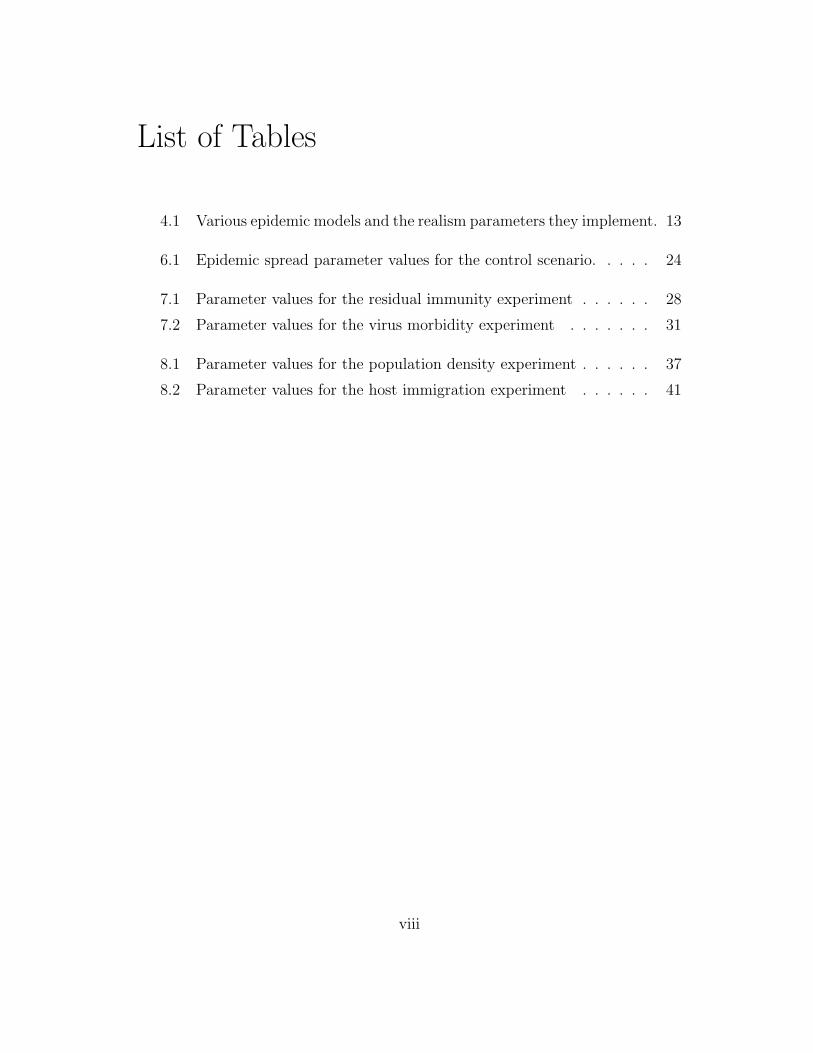
As stated earlier, a cell’s next state will depend on the current state of its neigh-bours. Before deciding on its next state, a cell will interrogate its neighbours fortheir present states and then evolve accordingly. Once again the size and shapeof the interaction neighbourhood is up to the implementer and will vary fromapplication to application. Figure 3.2 shows some of the more commonly usedneighbourhoods.

Figure 3.2: The black dot represents the target cell – the shaded cells are itsneighbours. The grid on the left shows the 4-connected, Von Neumann neigh-bourhood. The centre grid shows the 8-connected, Moore neighbourhood. Theright-hand neighbourhood uses a hexagonal lattice to provide equal separationsbetween cells.

9

CHAPTER 4

Review of the Literature

Epidemic spread models are devised for a number of reasons. Epidemiologistswant to create simple models so they can test the impact of specific parameterson an epidemic’s overall behaviour. Computer scientists might want to createsoftware packages that accurately depict the behaviour of epidemics as seen innature. The latter is the motivation for this dissertation.

There exist many models of epidemic spread, each with its own approach andset of assumptions. However, these models all share one property: the virtualworld in which they run is an idealized one where noise and imperfections arefiltered out. This arises from the difficulty of incorporating all the variables wesee in nature into a simulation that has a reasonable execution time — hoursrather than days. When modelling a complex system there is a trade off betweena model’s degree of abstraction and its usefulness; that is, without devaluing theresults a model provides, which details can be left out?

In this chapter I examine some of the existing epidemic modelling techniquesand compare their levels of detail and realism. The majority of past approacheshave used ordinary and partial differential equations (ODE’s and PDE’s). Iexamine those as well as mean field type (MFT) approximations [18] and cellularautomata (CA).

4.1 Parameters that influence epidemic spread

The main focus of my project is on the spatial behaviour of epidemics rather thanabsolute numbers and densities of infected individuals. In order to objectivelycompare the relative usefulness of modelling approaches I use a set of standardcriteria. These criteria are based on the following factors that Mollison [19]describes as significant in determining epidemic spread:

• susceptible population size,

10

• homogeneity of population density,

• infection transmissibility,

• immunity levels of individuals,

• motion of individuals, and

• infection incubation time.

All of the above will influence whether an infection will rapidly propagatethrough a population or head into extinction. Different models have differentassumptions regarding the above parameters and hence have different successrates in mimicking nature. The rest of this chapter examines three modellingmethodologies: ODE’s and PDE’s, MFT approximations, and CA to contrasthow each approach incorporates the above listed epidemic spread parameters. Amodel’s omission of a parameter does not necessarily imply that the model isunrealistic, though it might mean that the model is designed to investigate theimpact of one particular parameter independently of the others.

4.2 Differential equation models

Deterministic approaches to modelling, such as those using ODE’s and PDE’s,are poor at representing small populations compared to probabilistic models suchas CA [22]. They are poor in the sense that the results from ODE’s diverge tounreasonable values as the population size is scaled down toward zero. Thisdivergence is due to the simplifying assumptions made in ODE models:

• Population sizes are constant: no births, deaths or immigration occurs inthe world.

• Populations are uniformly distributed over the world.

• Populations are well mixed, that is, there is homogeneous motion about theworld.

Most of the above assumptions arise from regarding susceptible populations ascontinuous entities rather than comprising discrete individuals. Boccara [7] statesthat by recognizing that the spatial behaviour of an epidemic is “strongly linkedto the short range character of the infection process”, continuous differential

11

equation models that neglect the individual are probably going to be misleadingon all scales, not just small.

However, Di Stefano [22] shows that the continuous nature of ODE approx-imation is well suited to dealing with large populations because the effect ofthe close contact between individuals becomes negligible compared with the epi-demic’s macroscopic behaviour. The local correlations are lost because individu-als are able to roam all over the world. This spatial mixing effect is introducedinto PDE models through a diffusion term and become a function of the initialand boundary value conditions.

The need for homogeneity in an ODE model means that the natural pro-gression of an epidemic is not represented accurately. Variations in localizedpopulation densities, variations in immunity and susceptibility, and variations inincubation and sickness time are all attributes of natural epidemics but omittedin ODE simulations. Given that many spatial properties of epidemics are notrealized by differential equation models, another paradigm should be chosen ifspace issues are to be accurately addressed.

4.3 MFT approximation

Closely related to ODE and PDE models are those using mean field type (MFT)approximation. Kleczkowski [18] proposed an epidemic model using MFT ap-proximations examining the spread of childhood measles.

MFT approximation ignores localized correlations making it similar to a dif-ferential equation model [8]. MFT models assume that susceptible populationdensity is uniform over the world, which is also similar to ODE/PDE models.Finally, MFT and ODE/PDE models share the assumption that hosts are capa-ble of diffusing around the world – that is, the population is well mixed. Despiteall these similarities, MFT approximations are significantly different from dif-ferential equation models in that their mixing parameter can be a probabilisticvariable. Unlike ODE’s where either all individuals diffuse or none at all, thedecision to move around the MFT world is independent among individuals.

Similar to CA, MFT approximations utilize a lattice structure to emulatethe spatial nature of epidemic spread. Each lattice site contains an individualwho can exist in one of several states. The set of possible existence states isdetermined by the epidemic model being used. Many groups [7, 8, 13] haveused MFT approximations as a point of comparison with the CA models theydevelop; particularly models investigating the effect of host motion. Noting thatMFT approximations neglect localized correlations, it appears meaningless to

12

compare them with CA models because CA models focus on the contact betweenindividuals. But as Kleczkowski [18] describes, MFT and CA models convergewhen the MFT mixing parameter tends to infinity – that is, when the worldcontains more disorder than correlation. This convergence is analogous to thesituation where differential equation and CA models converge when populationsize tends to infinity.

In the context of exhibiting realistic spatial behaviour, MFT approximationsare better than modelling with differential equations because by determininghost movement probabilistically, they manage to partially portray the stochasticfluctuations observed in nature.

4.4 Spatial models: CA

Epidemic spread in nature is a stochastic process, so it seems logical to use amodel that is probabilistic. According to Ahmed et al. [2], “[CA have] a significantrole in epidemic modelling since it can be shown that [they are] more general thanordinary and partial differential equations.” This section examines existing CAmodels and identifies which virus spread parameters they have chosen to includeand which they have chose to omit.

All of the models that I discuss in this section are based on the SIR modelsuperposed with CA. The letters in SIR correspond to the three states an individ-ual can exist in: susceptible, infective and recovered [1]. Susceptible individuals,or susceptibles, are ones who can contract the pathogen from already infectedinfective individuals. Infectives can later recover from this infection. There arevariants of this model that introduce other intermediate states. For example, inSEIR there is the ‘E’ state, representing exposed but yet to be infected individuals.

Criteria [13] [7] [22] [1] [8]Wrap around world × × × × ×

Variable population size ×

Uneven population density × × ×

Movement of hosts × × ×

Immunity after recovery ×

Variable susceptibility ×

Includes incubation time ×

Includes latency time ×

Table 4.1: Various epidemic models and the realism parameters they implement.

13

The rest of this chapter looks at the models of Duryea et al. [13], Di Stefano etal. [22], Ahmed and Agiza [1], and Boccara et al. [8] to see which epidemic spreadfactors they have chosen to incorporate into their models. Such factors includepopulation density, host susceptibility and immunity, virus transmissibility, andvirus infection times. The inclusion of these parameters will directly affect therealism of the simulations we generate – that is, they are parameters that addheterogeneity to the otherwise idealistic world that designers build models in.Table 4.1 shows the parameters each group has chosen to implement.

4.4.1 Variable population size

In nature, the population within a region is always changing. Internal events suchas births and deaths increase and decrease the population respectively. Externalfactors such as immigration and emigration have similar effects. Epidemic spreadis affected by this constant flux in susceptible hosts but very few models includethis flux. The reason perhaps lies in the difficulty to integrate such features intoa model, or more probably, these models have very specific applications wherepopulation variation is considered negligible.

Of the five groups mentioned here, only one, Boccara et al. [8], has chosen tomodel population flux. When the proportion of infectives in a population reachesa constant steady-state value we say that the infection has become endemic.Boccara et al. chose to include the death and birth rates to investigate how theseparameters affect the stability of such endemic states. Other models such as thoseby Di Stefano [22] focus on the movement and the heterogeneity of susceptibilityin populations and choose to abstract out the population size parameter.

4.4.2 Uneven population density

The model of Boccara and Cheong [7] tries to introduce variations in populationdensity by allowing host movement. In effect, the cell update function is dividedinto two phases: infection and motion. Once each cell has decided which of theSIR states it evolves into, it chooses a destination cell and moves there. This hasthe effect of generating a non-uniform landscape of susceptible hosts.

Ahmed and Elgazzar [2] also model variations in population densities by al-lowing host movement; more specifically, cyclic host movement. PDE models usea diffusion term that creates random host motion whereas a cyclic cell to cellmapping function in a CA model makes it possible to emulate regular periodichost movement. This is analogous to someone going from home to work, andthen back home again.

14

4.4.3 Variable susceptibility

Susceptibility, immunity, and transmissibility relate to how easily a contagion canpass between hosts. Probabilistic CA/SIR models can represent highly contagiousviruses by assigning a high probability of infection when susceptibles come incontact with the contagion. Although these parameters are usually staticallydefined as in the model proposed by Ahmed and Agiza [1], the rule-based natureof CA means that these parameters can be modified dynamically during run-time. A population’s innate immunity to infection has a significant impact onwhether a small outbreak grows into an epidemic or simply dies out; the modelby Ahmed and Agiza appears to solely address this susceptibility parameter andneglects the others to perhaps isolate its effects.

4.4.4 Incubation and latency time

The last parameters in Table 4.1 to be discussed are incubation and latency time;these two terms should not be confused. The distinction is outlined in Figure 2.1.Incubation time is defined as the length of time between an individual beinginfected and an individual showing signs of disease. The time lapse between beinginfected and becoming infective is known as latency. Both of these quantitiesare modelled by Ahmed et al. [1], however they do not discuss the significance ofthese times. Others fail to include these quantities in their models but Ahmed andAgiza suggest that these parameters have an accelerating impact on an epidemic’sspatial spread.

4.4.5 Conclusion

Most of the models examined in this chapter have a specific focus: they isolatea particular epidemic spread parameter and see its effect over the epidemic asa whole. As part of determining the suitability of CA to epidemic modelling, itwill be necessary to take these specific models and try to compose them into asingle generalized composite model. By examining the merits of this compositemodel we can endorse or reject the conjecture that CA is appropriate for epidemicmodelling.

15

CHAPTER 5

My Epidemic Model

The cell evolution in a cellular automaton follows an update function that takesthe state of a particular cell and its neighbours and determines the next state.This chapter outlines the cell and update rule definitions adopted in my epidemicsimulation as well as the epidemic parameters that are implemented. A moredetailed description of the software implementation of this model can be foundin Appendix A.

5.1 Cell Definition

The basic unit of computation in my simulation is the cell. Here, ‘cells’ areautomata cells and not biological cells. However, rather than representing a par-ticular area of space, the effective size of a cell will be determined by the epidemicspread parameters set by the user. For example, by defining a small value for themobility, the user is in effect simulating the increased difficulty of traversing acell that represents a large area compared to a cell that represents a small area.The concept of a cell needs to be differentiated from the hosts that live insidethe cell, as illustrated by the following five cell attributes:

• carrying capacity,

• total population,

• susceptible subpopulation,

• infective subpopulation, and

• recovered subpopulation.

The carrying capacity of a cell is used as a mechanism to limit the movementof hosts between cells. It is a mechanism used to prevent crowding within a

16

particular cell – comparable to a surface area. The number of newborns will alsobe dependent on whether a cell has reached its carrying capacity. Although theeffect of the land’s carrying capacity is not directly enforced in nature, for thepurposes of simulation, it is a straightforward way to encourage or attenuate themotion of individuals between cells.

Traditionally, such as in the CA of Jon Von Neumann [9], a single automatonoccupied each of the cells that constituted the larger cellular automaton. Ratherthan stipulate this, this model allows multiple individuals to dwell in one cell upto the above-mentioned carrying capacity. Variable cell population has two mainpurposes: first it reduces the total number of cells and hence reduces computationtime; secondly it provides generality. If we set the carrying capacity to one wecan revert back to a traditional cellular automaton.

5.2 World Definition

A two–dimensional array of cells and the epidemic spread parameters that governtheir evolution constitute the world that the hosts ‘live’ in. The cells are arrangedin a rectangular grid comprising square cells with external dimensions that mayor may not be square. The world boundaries serve as impenetrable barriers tohost movement, but conceptually can be thought of as political boundaries thatallow immigration into and out of this world into adjacent worlds. The adjustableepidemic parameters that control cell evolution are described in the next section.

5.3 Adjustable Simulation Parameters

After researching existing epidemic models, particularly those examining viruspathogens that can survive outside the bodies of hosts, I compiled the followinglist of epidemic spread parameters. This is not an exhaustive list, but it containswhat I believe to be the most significant factors that account for the spatialbehaviour of an epidemic. Apart from the interaction radii, all the followingparameters are modelled using probabilities that directly impact the update rulesapplied over the CA lattice.

5.3.1 Neighbourhood radius

This parameter determines the size of the interaction neighbourhood that a cellinterrogates for state information. My simulation uses a square interaction neigh-

17

bourhood whose area, n, in terms of cells is determined by an interaction radius,r, as shown in Equation 5.1.

n = (2r + 1)2 (5.1)

There are two distinct interaction radii: motion and infection. The motionradius defines the greatest distance, measured in cells, a host can move during atime step. The infection radius is slightly different to the motion radius in thatit does not relate to hosts but to the virus pathogen. The infection radius definesthe greatest distance the virus pathogen can travel outside the body of a host onits own. This quantity is used to model the spread of a virus via natural vectorssuch as airborne droplets in influenza or vermin as in bubonic plague.

5.3.2 Motion probability

The individuals in the world are permitted to move between cells. The motionprobability determines the frequency of this motion. This simulation assumeshomogeneous mixing within each cell, but the motion of hosts between cells islimited by the motion probability parameter. For example, if the motion prob-ability, pmove, is set to 0.4, you would expect roughly two in five hosts to shiftfrom the cell they currently reside in to another cell within its motion neighbour-hood. The success of a host’s inter-cell movement is dependent on whether thedestination cell has reached its carrying capacity. In this model, the destinationcell is selected randomly from the surrounding interaction neighbourhood.

5.3.3 Immigration rate

This simulation can model an open or closed world, depending on the value of theimmigration parameter. For the purposes of this simulation, immigration refersto susceptible individuals who are not already in the world coming in and fillingany vacancies within the cell grid. This parameter determines the probabilitythat a cell will receive any immigrants. The actual number of immigrants willbe a random proportion of the number of spaces left in the cell. Immigration isequally likely for all cells except for cells which cannot support any more hosts(the cell is at its carrying capacity).

18

5.3.4 Birth rate

The birth rate parameter, as its name suggests, controls the addition of newbornsto the population pool at each time step. These increases are from births ofnew individuals via reproduction between existing hosts. It does not includepopulation increases due to immigration.

The birth rate is given as a parameter, pbirth, which is the probability thata pair of hosts will produce an offspring during a time step. The birth rate isuniform across all the possible different pair combinations such as SS, SI, SR, II,IR, and RR, but all newborns are susceptibles. That is, infection or immunity isnot passed onto the offspring. For many diseases this is a reasonable assumptionand makes the model simpler, but as discussed in Chapter 2 the contagion mightbe passed onto a child via vertical transmission. Equation 5.2 shows the relation-ship between the birth rate parameter and the total cell population increase pertime step.

% population increase per timestep ≈pbirth

2× 100 (5.2)

Equation 5.2 is only an approximation because births are determined proba-bilistically.

5.3.5 Natural death rate

Comparable to the birth rate parameter, deaths by natural causes are controlledby a natural death parameter. Unlike the birth parameter, the death parameterencompasses emigration from the world as well. This natural death parameterdoes not discern between the host types. That is, susceptibles, infectives andrecovered are equally affected by this parameter. The average lifetime of a healthyhost is approximated by the reciprocal of the natural death probability.

5.3.6 Virus morbidity

The neighbourhood radius, natural birth, immigration, and natural death pa-rameters mentioned above are all geographic or demographic factors that affectepidemic spread. Virus morbidity and the parameters discussed below are deemedviral spread factors.

Virus morbidity is a measure of how rapidly a virus kills its host, if at all.Unlike natural deaths, the virus morbidity parameter only affects infective hosts.

19

This parameter defines the probability that an infective will die from disease dur-ing a particular time step. For highly virulent viruses, the morbidity probabilitywill be close to unity, whereas very ‘mild’ viruses will have this parameter valuevery close to zero.

5.3.7 Vectored infection rate

Apart from entering an otherwise ‘clean’ cell inside a mobile infective host, thevirus contagion can spread across cells using its natural spreading mechanisms.Such spread is known as vectored infection. For this model, the velocity of inter-cell infection is controlled through the pinput parameter. The actual probabilityof spread, pvectored, is a function of the vectored infection parameter provided bythe user, pinput, and the density of susceptible hosts in the local interaction neigh-bourhood. This is illustrated in Equation 5.3. A high value for this parameterwould represent a highly transmissible virus such as one that was airborne orcarried in bird droppings.

pvectored =susceptible population

neighbourhood capacity× pinput (5.3)

5.3.8 Contact infection probability

Whilst the previous parameter handled the infection of hosts across cells, the con-tact infection probability determines how susceptible hosts are infected throughcontact with infectives within the same cell. Mixing within each cell is assumedto be homogeneous – all hosts in a cell will come in contact with all the otherhosts during a time step. The contact infection parameter is a measure of viruscontagiousness – highly contagious viruses need only a small amount of exposurebetween infective and susceptible hosts to pass on the contagion.

5.3.9 Spontaneous infection probability

To simulate the infection of individuals from factors external to the world, sus-ceptibles may be spontaneously ‘struck down’ with the virus. This parame-ter implies that although a susceptible individual might have escaped infectionthrough vectored and direct contact means, it might still become infective fromoutside means. Possibilities might include contracting the virus whilst on hol-idays, breathing in vermin faeces, contact with virus particles adhered to thetyres of vehicles, or other remote but still probable methods of infection. This

20

parameter is usually very small compared to the value of the other infectionprobabilities.

5.3.10 Recovery rate

In this simulation, recovery corresponds to a state change from infective to re-covered; it does not encapsulate death or emigration. Recovered individuals aresometimes known as removed individuals because they no longer contribute to theinfection cycle; not only are they immune from contracting the contagion, theycannot pass the contagion onto other susceptible hosts. The recovery rate param-eter is the probability that at a particular time step an infective host becomes arecovered host. The reciprocal of this parameter provides an approximation tothe mean infection duration.

5.3.11 Re–susceptible rate

The duration of a recovered host’s immunity is determined by the re-susceptibleparameter. This probability controls the chance of a recovered individual as-similating back into the susceptible population – in effect it is a recovered hostbecoming a susceptible host again. For viruses that mutate rapidly, this parame-ter will be close to unity, whilst viruses that offer lifelong immunity after infectionwill have a re–susceptibility close to zero.

5.4 Cell update algorithm

The CA cell update function is used to evolve each cell to its next state. The cellupdate function takes as arguments all the parameters outlined in the previoussection along with the state information of the interaction neighbourhood of thecell in question. The update of the world is done in two phases: first the motionof individuals between cells, then the evolution of individuals within cells.

5.4.1 Movement phase

1. Select a random cell from the world.

2. For each of the individuals in the cell, randomly select a neighbouring celland move the individual into it. This movement is dependent on the the

21

motion probability parameter described earlier and the destination cell notbeing full.

3. Repeat from step one until all the cells in the world have been accountedfor.

5.4.2 Infection and recover phase

1. Select the first cell.

2. Deduct the ‘natural deaths’ from the cell population.

3. Deduct the deaths from virus morbidity.

4. Add to the population any newborns.

5. Add any immigrant population.

6. Compute inter-cell (vectored) infections.

7. Compute intra-cell (contact) infections.

8. Compute spontaneous infections.

9. Compute host recoveries.

10. Compute re-susceptibles.

11. Repeat from step one for the next cell until all cells have been accountedfor.

22

CHAPTER 6

Control Scenario

Whenever a model of a natural phenomenon is devised, it needs to be calibratedsuch that any numbers that we supply as input or receive as output can be readilyinterpreted as ‘real-life’ figures. However, creating a fully calibrated model isbeyond the scope of this project as I am only interested in examining whetherCA is a good starting point for a comprehensive model. To substitute calibration,I have devised a control scenario which will be used as a comparison for all theexperiments discussed later.

6.1 World setup

The control world comprises a 100 × 100 grid of cells, with each cell possessingthe characteristics described in Chapter 5. Each cell will start with a populationof 100 susceptibles and be capable of supporting a maximum of 200 individuals.There is no initial source of infectives. The world starts ‘clean’ and waits forspontaneous outbreaks to spark an epidemic. A point source of infectives wasnot used because later experiments rely on spontaneous infections to seed theepidemics. This is to try and emulate how epidemics start in nature.

6.2 Parameter settings

The control scenario represents a homogeneously distributed population wherethe total population is in a state of dynamic equilibrium – that is, the num-ber of births roughly balances the number of deaths. However, the populationis expected to gradually increase due to immigration from outside worlds. Anon-zero motion probability means that at each time step, it is expected thatapproximately 0.1% of individuals will attempt to shift out of their current cellinto another one in their interaction neighbourhood. The initial values of theepidemic spread parameters described in Chapter 5 are summarized in Table 6.1.

23

Parameter Value InterpretationInfection radius 1 adjacent spread onlyMovement radius 1 adjacent movement onlyImmigration rate 0.01 1% increase in population per time stepBirth rate 0.02 1% increase in population per time stepNatural death rate 0.01 1% decrease in population per time stepVirus morbidity 0.05 5% of infectives die per time stepSpontaneous infection rate 0.0001 1 in 10000 chance of outside infectionVectored infection rate 0.2 20% chance of hostless inter–cell spreadContact infection rate 0.4 2 in 5 chance of infection after close contactRecovery rate 0.1 10% of infectives recover per time stepResusceptible rate 0.001 residual immunity lasts ≈1000 time stepsMovement probability 0.001 1 in 1000 individuals attempt to shift cells

Table 6.1: Epidemic spread parameter values for the control scenario.

Whilst it is simple to define a typical host population, it is much more difficultto define a typical virus strain for the control scenario without losing generality.To that end, although the values in Table 6.1 do not quantitatively representa particular virus, the ratios between the parameters need to be reasonable.Essentially these numbers are just educated guesses at what a typical virus wouldbe.

6.3 Results

Figure 6.1 shows the fluctuation in the proportion of infectives in the world over800 time steps. It is important to note that after approximately 100 epochs,the proportion of infectives levels out. I will define this steady-state value as anendemic level of infection in the population.

The plot in Figure 6.2 provides an indication of the dynamics of the totalpopulation, not just the infective hosts. Starting from an initial population ofone million the population rises by approximately 12% and at about the fifti-eth epoch the population starts to fall sharply to a much smaller value than itstarted. A comparison of Figures 6.1 and 6.2 shows that the rapid decline in pop-ulation corresponds to the sharp increase in infectives. The population reachesa local minimum just before the hundredth epoch and then starts to regenerate.This regeneration corresponds almost exactly with the point in Figure 6.1 whenthe proportion of infectives bottoms out. As the population recovers it reaches

24

0 100 200 300 400 500 600 700 8000

0.1

0.2

0.3Control scenario

Time (epochs)

Pro

port

ion

of in

fect

ives

Figure 6.1: The proportion of the total population that is infective during thecontrol scenario. From an initial infective population of zero, the infection spreadsrapidly before peaking at ≈ 0.26. From there, the transient rapidly decays andreaches an endemic proportion of ≈ 0.1.

a steady state value which is roughly one million – its initial size before theepidemic.

6.4 Discussion

The shape of the graph in Figure 6.1 is one which will be seen often in later ex-periments. The initial surge in infectives is a result of the virus spreading rapidlythrough a purely susceptible population with no natural immunity. However, ashosts recover and acquire immunity, the number of infectives quickly reduces toan endemic level. For any subsequent epidemics to occur the population will needto lose its natural immunity or be injected with a large number of infectives.

This control experiment provides some initial evidence for the suitability ofCA for epidemic modelling. The dynamics seen in Figure 6.1 are similar to thosepresented by Boccara et al. [8] and Kleczkowski [18] in their models that usemean field type approximations. However, they do not mention whether theyhave used real life data to validate the results from their theoretical models.

The main purpose of this experiment is to provide a benchmark for the fol-lowing experiments. As parameters and initial conditions are varied in later

25

0 100 200 300 400 500 600 700 8000.85

0.9

0.95

1

1.05

1.1

1.15x 10

6 Control scenario

Time (epochs)

Tot

al p

opul

atio

n

Figure 6.2: The fluctuation of the total world population over 800 time steps.After some rapid growth in the first 50 time steps the population declines just asrapidly. This decline corresponds with the peak in Figure 6.1. From time = 100onward, the population recovers to roughly its original size.

experiments, new results can be interpreted with respect to the results presentedhere and their consequences discussed.

26

CHAPTER 7

Viral Parameter Experiments

This section investigates whether a CA epidemic model can encapsulate the ca-pabilities of existing, non-spatially oriented models. Specifically the viral param-eters of immunity and virulence are examined. Each of these experiments hasthe same starting state as the control scenario, except that some of the viralparameters will be different.

7.1 Residual immunity

A population’s natural immunity to a viral contagion will limit the chances of asmall outbreak escalating into a large scale epidemic. There are many so-called‘childhood diseases’ such as chicken pox and measles where exposure and recoveryprovides the host with extended immunity. The duration of this immunity variesfrom one virus strain to another because even though a host may produce anti-bodies to fight further infection, the virus may mutate into a more resilient strain.This experiment does not examine the mutation rate of a virus (it assumes thatthere is only one strain) rather it looks at how immunity can be implemented ina CA model.

7.1.1 World setup

The world in this experiment is identical to the uniform world described in thecontrol scenario described in Chapter 6. Each cell has a carrying capacity of200 and an initial population of 100 susceptibles. Being free of infectives, anyvirus outbreaks in this world will be due to the non-zero spontaneous infectionparameter.

27

7.1.2 Parameter settings

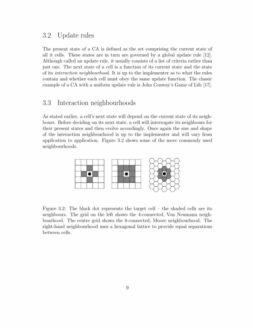
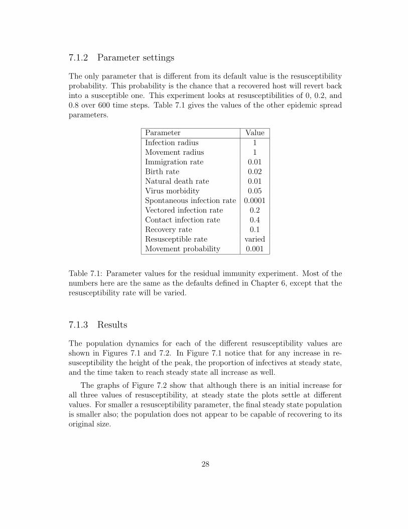
The only parameter that is different from its default value is the resusceptibilityprobability. This probability is the chance that a recovered host will revert backinto a susceptible one. This experiment looks at resusceptibilities of 0, 0.2, and0.8 over 600 time steps. Table 7.1 gives the values of the other epidemic spreadparameters.

Parameter ValueInfection radius 1Movement radius 1Immigration rate 0.01Birth rate 0.02Natural death rate 0.01Virus morbidity 0.05Spontaneous infection rate 0.0001Vectored infection rate 0.2Contact infection rate 0.4Recovery rate 0.1Resusceptible rate variedMovement probability 0.001

Table 7.1: Parameter values for the residual immunity experiment. Most of thenumbers here are the same as the defaults defined in Chapter 6, except that theresusceptibility rate will be varied.

7.1.3 Results

The population dynamics for each of the different resusceptibility values areshown in Figures 7.1 and 7.2. In Figure 7.1 notice that for any increase in re-susceptibility the height of the peak, the proportion of infectives at steady state,and the time taken to reach steady state all increase as well.

The graphs of Figure 7.2 show that although there is an initial increase forall three values of resusceptibility, at steady state the plots settle at differentvalues. For smaller a resusceptibility parameter, the final steady state populationis smaller also; the population does not appear to be capable of recovering to itsoriginal size.

28

0 100 200 300 400 500 6000

0.1

0.2

0.3

0.4

0.5

0.6

0.7Residual immunity

Time (epochs)

Pro

port

ion

of in

fect

ives

p = 0p = 0.2p = 0.8

Figure 7.1: The proportion of total population that is infective over 600 timesteps. The probability of resusceptibility is set to p = 0, p = 0.2, and p = 0.8. Asthe resusceptibility probability is increased, the duration of the epidemic (signi-fied by the width of the peak) and the level of endemic infection also increases.

0 100 200 300 400 500 6000

2

4

6

8

10

12x 10

5 Residual immunity

Time (epochs)

Tot

al p

opul

atio

n

p = 0p = 0.2p = 0.8

Figure 7.2: The fluctuations in total population for the same world as in Fig-ure 7.1. As the resusceptibility probability is increased from 0 to 0.2 to 0.8, thereis a reduction in the total steady-state population. Note that each graph reachesapproximately the same maximum, but have markedly different populations whenthe virus has decayed to its endemic level.

29

7.1.4 Discussion

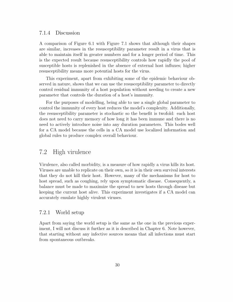
A comparison of Figure 6.1 with Figure 7.1 shows that although their shapesare similar, increases in the resusceptibility parameter result in a virus that isable to maintain itself in greater numbers and for a longer period of time. Thisis the expected result because resusceptibility controls how rapidly the pool ofsusceptible hosts is replenished in the absence of external host influxes; higherresusceptibility means more potential hosts for the virus.

This experiment, apart from exhibiting some of the epidemic behaviour ob-served in nature, shows that we can use the resusceptibility parameter to directlycontrol residual immunity of a host population without needing to create a newparameter that controls the duration of a host’s immunity.

For the purposes of modelling, being able to use a single global parameter tocontrol the immunity of every host reduces the model’s complexity. Additionally,the resusceptibility parameter is stochastic so the benefit is twofold: each hostdoes not need to carry memory of how long it has been immune and there is noneed to actively introduce noise into any duration parameters. This bodes wellfor a CA model because the cells in a CA model use localized information andglobal rules to produce complex overall behaviour.

7.2 High virulence

Virulence, also called morbidity, is a measure of how rapidly a virus kills its host.Viruses are unable to replicate on their own, so it is in their own survival intereststhat they do not kill their host. However, many of the mechanisms for host tohost spread, such as coughing, rely upon symptomatic disease. Consequently, abalance must be made to maximize the spread to new hosts through disease butkeeping the current host alive. This experiment investigates if a CA model canaccurately emulate highly virulent viruses.

7.2.1 World setup

Apart from saying the world setup is the same as the one in the previous exper-iment, I will not discuss it further as it is described in Chapter 6. Note however,that starting without any infective sources means that all infections must startfrom spontaneous outbreaks.

30


To isolate the effect of the virus morbidity parameter on epidemic spread, all ofthe parameters described in Chapter 5 are set to their default values. For thisexperiment virus morbidity is set to 0.5: it is expected that at each time stephalf of the infective individuals will die. This represents a highly virulent virussuch as some strains of Ebola found in the developing countries of Africa [24].The epidemic spread parameters are summarized in Table 7.2.

Parameter ValueInfection radius 1Movement radius 1Immigration rate 0.01Birth rate 0.02Natural death rate 0.01Virus morbidity 0.5Spontaneous infection rate 0.0001Vectored infection rate 0.2Contact infection rate 0.4Recovery rate 0.1Resusceptible rate variedMovement probability 0.001

Table 7.2: Parameter values for the virus morbidity experiment. A virus mor-bidity value of 0.5 represents a virus that on average kills within two epochs ofinfection.

7.2.3 Results

The graph in Figure 7.3 shows that after a rapid increase in the proportion ofinfectives (numbers reach approximately 8% of the total population), there is asimilarly steep decay back down to approximately 1.5%. From about t = 100onwards, the graph becomes very jagged where values fluctuate between 2.5% and4.5%. There are distinct troughs and peaks in the graph where a local maximumis followed by a local minimum less than 10 time steps later. This jagged patternis superposed with a larger pattern with a period of approximately 50 time steps,seen more clearly after t = 500. However, there does not appear to be any clearperiodicity elsewhere.

31

0 100 200 300 400 500 600 700 8000

0.01

0.02

0.03

0.04

0.05

0.06

0.07

0.08Highly virulent virus

Time (epochs)

Pro

port

ion

of in

fect

ives

Figure 7.3: A virus that has high virulence (or morbidity) will kill a high propor-tion of infective hosts before they can recover. This plot shows a virus infectingthe control population described in Chapter 6 with a resusceptibility of 0.001 andmorbidity of 0.5 executed over 800 time steps.

0 100 200 300 400 500 6000

1

2

3

4

5

6

7

8

9

10

11x 10

5 Highly virulent virus

Time (epochs)

Tot

al P

opul

atio

n

Figure 7.4: A similar plot to Figure 7.3 except that it shows total population notjust infectives. Once again there appears to be an underlying oscillatory natureto the curve.

32

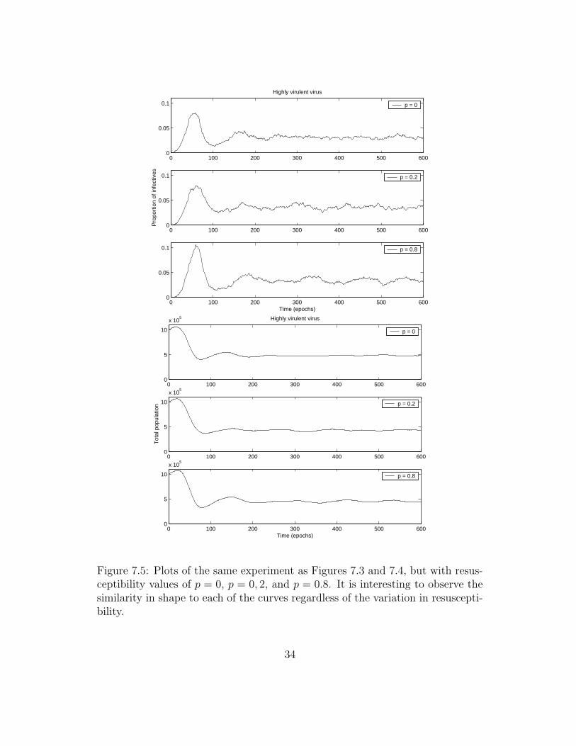
Figure 7.4 does not show the same jagged characteristics of Figure 7.3. How-ever, after the initial population decay the graph seems to settle into an oscilla-tory pattern. To show that this oscillatory pattern is not a result of coincidence,I have repeated this same experiment but with resusceptibility probabilities of0, 0.2, and 0.8. The results are presented in Figure 7.5. Notice that at leastqualitatively, each set of three graphs looks very similar.

7.2.4 Discussion

A highly virulent virus that kills its host quickly is unlikely to successfully spreadto a new host [3]. This effect is shown by the much reduced numbers of Figure 7.3in relation to the control scenario of Chapter 6. The jagged nature of this graph,not present in the control scenario, is due to the sudden death of many infec-tives during a particular time step. This periodicity has been observed in closedpopulations such as those on found on the Faroe Islands [20]. The quasi-periodicnature of the curve results from the regular injection of new susceptibles (new-born or immigrant) that provide the epidemic with new hosts only to later havethese new hosts die from the infection a few time steps later.

The similarities in the graphs of Figure 7.5 suggest that changing the residualimmunity of hosts has no significant effect when dealing with a highly virulentvirus. The effect of the immunity parameter appears to be negligible comparedwith the influence of the virulence parameter. This makes sense because the viruskills so swiftly that recoveries are few. In nature it is probably difficult to finda virus that kills rapidly and yet provide the survivors with lifelong immunity.This is because both of these characteristics work against virus spread and wouldnot be deemed advantageous mutations during natural selection.

This experiment shows how some emergent behaviours of epidemics such asperiodicity have been captured in a simple CA model. Specifically, this period-icity is encapsulated into a single parameter: the virus morbidity. Although it isthe ability of CA to incorporate space into epidemic models that is under ques-tion, showing that a CA model can reproduce the statistical results as observedin nature provides us with some confidence in CA as a modelling approach ingeneral.

33

0 100 200 300 400 500 6000

0.05

0.1

Highly virulent virus

p = 0

0 100 200 300 400 500 6000

0.05

0.1

Pro

port

ion

of in

fect

ives

p = 0.2

0 100 200 300 400 500 6000

0.05

0.1

Time (epochs)

p = 0.8

0 100 200 300 400 500 6000

5

10

x 105 Highly virulent virus

p = 0

0 100 200 300 400 500 6000

5

10

x 105

Tot

al p

opul

atio

n p = 0.2

0 100 200 300 400 500 6000

5

10

x 105

Time (epochs)

p = 0.8

Figure 7.5: Plots of the same experiment as Figures 7.3 and 7.4, but with resus-ceptibility values of p = 0, p = 0, 2, and p = 0.8. It is interesting to observe thesimilarity in shape to each of the curves regardless of the variation in resuscepti-bility.

34

CHAPTER 8

Spatial Experiments

The focus of this dissertation is on the spatial aspects of epidemics, particularlyhow spatial parameters affect the way they spread. This chapter contains aseries of experiments that show how a CA model can emulate several emergentbehaviours of an epidemic yet use only one rule set. The results of the experimentsin this chapter provide a basis for deciding the suitability of CA to epidemicspread modelling.

8.1 Varied population density

A virus relies upon a supply of susceptible hosts to survive and replicate. Butbefore a virus can infect a new host it must come in contact with it. An indi-cator to whether an outbreak will spread is the basic reproductive number, R0,discussed in Chapter 2. According to Equation 2.2, R0 is directly proportional tothe number of contacts per unit time which itself is proportional to the local pop-ulation density. Therefore, in regions of high local population density we expectan epidemic to spread more rapidly than in low density regions. This experimentexamines the effect of varied local population density and how CA rules can beused to emulate those effects.

8.1.1 World setup

This experiment is broken down into two sub-experiments. To juxtapose theeffect of local population density on virus infection velocity I have used twosynthetic landscapes – one with a negative density gradient from top to bottom,and another with a positive density gradient from top to bottom. These areshown in Figures 8.1 and 8.2. Those figures also show the initial ‘line source’ ofinfectives at the top of the grid. It is assumed that during the early stages ofthe experiment the epidemic spreads through the top of the grid and during thelater stages spreads through the lower part of the grid.

35

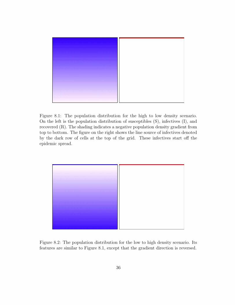
Figure 8.1: The population distribution for the high to low density scenario.On the left is the population distribution of susceptibles (S), infectives (I), andrecovered (R). The shading indicates a negative population density gradient fromtop to bottom. The figure on the right shows the line source of infectives denotedby the dark row of cells at the top of the grid. These infectives start off theepidemic spread.

Figure 8.2: The population distribution for the low to high density scenario. Itsfeatures are similar to Figure 8.1, except that the gradient direction is reversed.

36


To isolate the effect of local susceptible population density on the spread of anepidemic, most of the other parameters in this experiment are set to zero. Thisis to remove any skew that may arise from including several factors at once.The vectored and contact infection parameters are set to unity to accelerate thespread of the virus; doing this should not adversely affect the results because itis not the absolute value of the infection velocity that is of concern, but how itchanges with respect to population density. The recovery probability is set tozero so that the epidemic spreads in one direction only – that is, velocity cannotbe negative.

Additional to using a ramped population density, this experiment will lookat the effects of increasing the interaction neighbourhood size of the local pop-ulation density, as defined in Equation 8.1. Consequently, changing the size ofthe interaction neighbourhood will also change the local population density. Thevalues of the other parameters are summarized in Table 8.1.

local population density =neighbourhood population

neighbourhood capacity(8.1)

Parameter ValueInfection radius variedMovement radius 0.0Immigration rate 0.0Birth rate 0.0Natural death rate 0.0Virus morbidity 0.0Spontaneous infection rate 0.0Vectored infection rate 1.0Contact infection rate 1.0Recovery rate 0.0Resusceptible rate 0.0Movement probability 0.0

Table 8.1: The parameter values for the population density experiment. Mostof the parameters are set to zero except for the ones that relate directly topopulation density. For this experiment, the infection radius is varied and itseffect examined. Note that both the high to low density scenario and the low tohigh density scenario use the same parameter values.

37

8.1.3 Results

Each of the plots in Figures 8.3 and 8.4 show the proportion of the total pop-ulation that is infective over the course of 100 epochs or iterations. There aretwo features of note for each plot of each figure: the plot’s gradient and the timebefore the population becomes saturated with infectives.

For the high to low density scenario in Figure 8.3, we can see that the gradientsof the plots start off much steeper than they finish. That is, as the populationdensity decreases so does the gradient. A similar effect can be seen for thelow to high density scenario in Figure 8.4. Each of the curves starts with ashallow gradient, or small infection velocity, and as the epidemic reaches thehigher density regions, the gradients steepen.

When the infection radius is increased the population becomes saturated withinfectives more rapidly. That is, the ‘wave’ of infection reaches the bottom of thegrid in less time.

0 10 20 30 40 50 60 70 80 90 1000

0.1

0.2

0.3

0.4

0.5

0.6

0.7

0.8

0.9

1High density to low density

Time (epochs)

Pro

port

ion

of in

fect

ives

r = 1r = 2r = 5r = 10

Figure 8.3: Effect of population density on epidemic spread velocity. For theearlier time steps, we see the gradient of the graph is much steeper than for thelatter time steps. Each of the graphs corresponds to a different infection radius,r. Notice that for increasing infection radius the gradients become steeper.

38

0 10 20 30 40 50 60 70 80 90 1000

0.1

0.2

0.3

0.4

0.5

0.6

0.7

0.8

0.9

1Low density to high density

Time (epochs)

Pro

port

ion

of in

fect

ives

r = 1r = 2r = 5r = 10

Figure 8.4: Similar scenario to Figure 8.3, but for a different CA starting state.This plot appears to be opposite to the previous scenario: here the transientfinishes much steeper than it starts. Each of the graphs corresponds to a differentinfection radius, r.

8.1.4 Discussion

The infection velocity of the epidemic is proportional to the gradient of the plotsin Figures 8.3 and 8.4. As expected, as the epidemic spreads through a highdensity region, the infection velocity is greater than for low density regions. Innature, this effect is attributed to the increased number of contacts between aninfective host and other susceptible hosts, as shown in Equation 2.2.

As the size of the infection interaction neighbourhood is increased there is anarrowing effect on the graph: the virus propagates through the population morerapidly, but still exhibits the velocity changes noted earlier. This acceleration ininfection is mostly due to the larger ‘reach’ a contagion has to infect hosts inother cells. For example, viruses that are airborne or spread by birds would havea high ‘reach’ or transmissibility.

From a modelling perspective, the two curves of Figures 8.3 and 8.4 are ex-actly as predicted by epidemic theory – that is, high densities promote rapidspread. This experiment has shown that a CA model can take into account thelocal population profile and produce the appropriate epidemic spread velocity.This partially justifies CA as a good epidemic modelling paradigm in that wehave shown that the ruleset I devised for my model produces the desired results.

39

However, as yet we have no assurances that these rules will work for more complexlandscapes.

8.2 Host immigration

Whilst the experiment that examined variations in population density had thedensity profile remain static for the duration of the experiment, this experimentlooks at the effect of dynamic variations in population density and composi-tion. Of particular interest are the variations due to host immigration. Althoughnot purely a spatial factor, immigration affects the population density and dis-tribution over the landscape, indirectly influencing the spatial behaviour of anepidemic.

8.2.1 World setup

This experiment uses the exact same initial setup as the control scenario describedin Chapter 6 where the population is uniformly distributed over the landscape.Each cell starts with a population of 100 susceptibles and has room to fit 100more SIR hosts.


Once again this experiment is broken down into two sub-experiments. However,instead of using different starting landscapes, this experiment uses two differentsets of spread parameters. Most of the parameters are initialized to the defaultvalues defined in Chapter 6 except of course for the immigration rate. To simulatea closed population, the immigration rate is set to zero – there are no incominghosts from outside the world. For an open population, this parameter is set to0.05, meaning that approximately 5% of cells will receive susceptible hosts froman external source to fill up some of its empty space. The values of the otherparameters are shown in Table 8.2.

8.2.3 Results

The results for the closed population are displayed in Figure 8.5. It shows thefamiliar shape of an initial virus outbreak that decays back down to a smallersteady state value. The simulation was run for 800 epochs and for four different

40

Parameter ValueInfection radius 1Movement radius 1Immigration rate (closed) 0.0Immigration rate (open) 0.05Birth rate 0.02Natural death rate 0.01Virus morbidity 0.05Spontaneous infection rate 0.0001Vectored infection rate 0.2Contact infection rate 0.4Recovery rate 0.1Resusceptible rate variedMovement probability 0.001

Table 8.2: The epidemic spread parameters used in the host immigration ex-periment. Most of the values here are the same as in Table 6.1 except for theimmigration probability which is 0 for the closed scenario and 0.05 for the openscenario. Part of this experiment will look at the effects of residual immunitycontrolled by the resusceptibility parameter.

values of resusceptibility: 0, 0.1, 0.5, and 0.9. As the chance of resusceptibilityis increased there is a corresponding increase in the maximum ratio betweeninfectives and total population.

In each case, the proportion of infectives decays down to a value very close tozero. However, it is interesting to note that although for values of resusceptibilityequaling 0.1, 0.5, and 0.9 the infective population decayed to zero by t = 300,when the resusceptibility was set to zero, the infective population did not reachzero until much later.

The results for the open population shown in Figure 8.6 are much more con-sistent. Although the simulation was run for 800 epochs, only the first 400 areshown here as the infections rapidly reached steady state. The main feature tonote is that all of the plots reach a non-zero steady state value. Increases inthe resusceptibility parameter have resulted in a corresponding increase in theproportion of infectives at steady state, as well has removing the distinct peakthat represents the epidemic.

41

0 100 200 300 400 500 600 700 8000

0.1

0.2

0.3

0.4

0.5

0.6

0.7Closed population

Time (epochs)

Pro

port

ion

of in

fect

ives

p = 0p = 0.1p = 0.5p = 0.9

Figure 8.5: A closed population does not allow outside individuals to enter theworld. From the graph above we see that after the initial outbreak peaks anddecays to zero, the infection does not become endemic. Each of the plots corre-sponds to a resusceptibility probability of p = 0, p = 0.1, p = 0.5, and p = 0.9.Notice that for increasing resusceptibility, the number of hosts that become in-fected during the epidemic (the hump) increases dramatically.

0 50 100 150 200 250 300 350 4000

0.1

0.2

0.3

0.4

0.5

0.6

0.7

0.8

0.9Open population

Time (epochs)

Pro

port

ion

of in

fect

ives

p = 0p = 0.1p = 0.5p = 0.9

Figure 8.6: An open population allows the free movement of individuals in andout of the world. These graphs show a plateau structure as the resusceptibilityprobability is increased from 0 to 0.9. In contrast with Figure 8.5, all of the plotsreach an endemic non-zero value.

42

8.2.4 Discussion

Historical evidence has shown that for a population in which individuals arealways coming and going there is a greater chance that an infection will becomeendemic after an outbreak [21]. Conversely, for isolated communities, it is usuallythe case that after an initial outbreak, the immunity acquired by the survivorslimits any chance of a virus continuing to be active [20]. The reason for the effectmentioned by Scott and Duncan [21] is that in an open population, the virus canrely upon a constant influx of new susceptible hosts. On the other hand, remotepopulations such as those on islands or in isolated villages provide the virus withno new hosts and usually results in the virus’ demise.

The results presented in this section partially portray the effect of immigra-tion on endemic infection, but other anomalies make it hard to draw any otherconclusions. Quantitatively, the results are very extreme: an endemic proportionof 70% is highly unlikely – such large figures clearly show the limitations an un-calibrated model. Qualitatively, we are still able to see the expected increase inendemic infection with an increase in resusceptibility, so I believe there is stillenough evidence to justify the development of a composite CA epidemic model.

8.3 Corridors of spread

This experimental scenario is the first of two that will use my CA model to tryand visualize how an epidemic would spread through a more complex virtuallandscape than that seen earlier.

8.3.1 World setup

This experiment tries to reproduce what might be a real life landscape withimaginary town centres and transport links between them. I use ‘towns’ and‘roads’ because they are human influenced and attract high population densities.The scenario is not restricted to cultural features; other natural features such asrivers might lead to development along their shores. Conversely, other geograph-ical features such as mountain ranges or swamps will limit development. Whatis important is their directed and linear shape rather than the wide sweepingpopulation densities used in previous experimental scenarios. Figure 8.7 showsthe virtual landscape used in this experiment.

Each cell has a carrying capacity of 1000, with three ‘towns’ already at thismaximum. Two of these towns, the north-west one and the south-east one,

43

Figure 8.7: The synthetic landscape that I devised to show how an epidemic islikely to spread along features of high density before spreading across open space.There are three points of high population density – two of which are connected bya transport link which has its own settlement developed on either side of it. Thenorth-west and south-east ‘towns’ both have 100 infectives and 900 susceptibles.

start with a 1:9 infective to susceptible ratio. The ‘transport links’ comprise athree cell wide bar of susceptibles. Cells on the central axis of this bar havean initial susceptible population of 100, whilst the cells on either side have aninitial susceptible population of 75. The rest of the landscape comprises cellswith 10 susceptibles in them. The town in the south-west corner contains 1000susceptibles and no infectives.


The parameter settings for this scenario, because I am looking at the directedspread of the epidemic with respect to population density, are the same as forthe high to low, and low to high scenarios discussed earlier. Table 8.1 liststhe parameter values: essentially all of the parameters are zero except for theinfection radius, contact infection probability, and vectored infection probabilitywhich are all equal to one.

8.3.3 Results

The results of this scenario are presented in the lag map shown in Figure 8.8. Thelag map is basically a series of snapshots taken at t = 0, 20, 40, 60, 80, 100, 200, 300.

44

Each cell is represented by a coloured square: red squares contain at least oneinfective host and white squares contain only susceptible and recovered hosts.Figure 8.8 shows the tendency of the epidemic to follow the lines of populationdensity to produce the ‘fuzzy cross’ pattern.

After 300 epochs, the top left outbreak has reached all four edges of the mapbut the bottom right outbreak is yet to reach any. Notice that the epidemicspreads outward along the arms or ‘roads’ before filling up the space between theroads.

8.3.4 Discussion

This particular scenario provides some evidence of the power of CA models forvisualizing an epidemic; differential equation models provide no such capability.In Figure 8.8 it becomes obvious to see where the infective towns were, where thedensest populations are situated, as well as identify where the infection velocityis greatest. Features such as leap frogging or infilling where the epidemic appearsto skip regions of land before coming back to fill in the space can be seen in thelag map. This behaviour was documented in the foot and mouth disease epidemicin Great Britain in 2002 [14].

Knowing beforehand the probable direction that an epidemic will take mighthelp public health officials efficiently direct containment measures and medicalservices to deal with infections.

8.4 Barriers to spread

The last experimental scenario in this chapter tries to show how a CA modelcan simulate the effects of erecting barriers to slow or stop virus spread. As seenin the foot and mouth disease epidemic in Great Britain during 2001, a key toslowing down disease spread is restricting movement. Other measures includedthe culling of livestock or the inoculation of livestock. I try to reproduce thesemeasures in this scenario by varying the initial state of the CA lattice.

8.4.1 World setup

Figure 8.9 shows the starting distribution with two squares that represent ‘cattle’farms. The top left farm has a four square wide barrier surrounding it, whereasthe bottom left farm has a one square wide barrier surrounding it. Barriers are

45

Figure 8.8: A lag map showing the state of the epidemic at t =0, 20, 40, 60, 80, 100, 200, 300. Notice that the outbreak to the north-west is ableto cover a greater distance than the outbreak in the south-east because it hasaccess to the road link and the population associated with that link. Notice thatthe spread from t = 20 in the top left of the map appears asymmetric. This isprobably an artifact of the stochastic nature of this model.

46

implemented as cells with zero carrying capacity. In Figure 8.9, barriers arerepresented by black squares and host occupation is represented by blue shading.

Figure 8.9: In this scenario there are two sources of infection, each with a differentsized barrier around it restricting host movement and providing no hosts for anyviruses that try to cross.


Apart from increasing the infection radius to two, there are no additional param-eter changes for this scenario – the default values used in the control scenario areused again. Having an interaction radius of two means that the barrier aroundthe infectives in the bottom right corner will still be able to disperse.

8.4.3 Results

The resultant epidemic spread is shown in the lag map of Figure 8.10. Noticethat the virus is able to elude containment in the bottom right ‘farm’. Despitethe farm itself becoming free of infectives, the neighbouring country side hasbecome infective. The upper left farm is no longer contaminated and neither isits surrounding hinterland.

47

Figure 8.10: This lag map shows that buffer zones that are too narrow provideno resistance to the spread of a virus.

48

8.4.4 Discussion

Much like the previous experiment, this scenario provides an opportunity todemonstrate the visualization capabilities of a graphical CA model. There are nonew epidemiological conclusions to be drawn from either of the last two experi-ments – they show exactly what our intuition would suggest. What is importantis that other statistical models do not appear to illustrate such behaviours verywell. As far as sample data is concerned, very little is available about the spatialbehaviour of epidemics; much of epidemiology looks at statistical data and try-ing to devise models that match that data. This is particularly the case with lagmaps where data is gathered during and after the epidemic, rather than beinggenerated preemptively.

What my project hopes to do is to provide a starting point for using CAmodels as a predictive tool for epidemiologists. The main hurdle to achievingthat goal is finding comprehensive data to calibrate and validate models.

49

CHAPTER 9

Conclusion

To improve their conformance to nature, models of naturally occurring phe-nomenon should consider all of the parameters believed to influence that phe-nomenon’s behaviour. However, to do so would result in highly complex and in-tractable models. Consequently, modellers must make simplifications that whilstmaking the model more tractable, do not seriously sacrifice accuracy.

For the case of epidemiology, there is scientific and anecdotal evidence sug-gesting that spatial heterogeneity has a significant effect over an epidemic’sspread [16, 23]. This dissertation has examined the application of cellular au-tomata (CA) to epidemic simulation, specifically its ability to capture the impactof localized variations in host population densities.

Two sets of experiments were conducted: the first investigating whether aCA could reproduce the macroscopic behaviour of epidemics as predicted byexisting models; the second set focused on whether a CA model could mimic thedependence of virus spread velocity on population distribution patterns. Theresults from each of these experiments was compared with those obtained from acontrol experiment. This comparison was used to highlight the effects that eachepidemic spread parameter had over the entire epidemic.

The first set of experiments dealt with two virus parameters: residual immu-nity and virus morbidity. Decreasing the residual immunity that hosts acquiredafter recovery (modelled by increasing the resusceptibility probability) had theeffect of increasing the endemic level of infection. Experimentation with high fig-ures for virus morbidity resulted in outbreaks that spread slowly with oscillatorybehaviour. Both of these outcomes reflect the observed behaviour in nature aswell as that predicted by other models.

The second set of experiments looked at mimicking the spatial behaviour ofepidemics. These synthetic scenarios showed that variations in infection veloc-ity caused by heterogeneous population density can be incorporated into a CAmodel by using a vectored infection parameter. The inter-cell infection rule usesthe local population density, defined by the size of the interaction neighbourhood,

50

to moderate the spread of infection. Consequently, as the size of the interactionneighbourhood is increased, the effect of localized interactions between the dis-crete hosts is lost and the model converges toward a continuous model.

Validation of my model involved isolating each epidemic spread parameter inits own test scenario and showing that its effect, relative to the control scenario,was what was seen in epidemic theory. Particular effort was made to test thespatial parameters, however data to validate the effect of these parameters isdifficult to find; epidemiology is traditionally a statistical field.

After testing each parameter in isolation, a composite scenario that repre-sented a ‘real-life’ landscape was used to test the model as a whole. The hy-pothesis is that the macroscopic behaviour of an epidemic can be represented bythe sum of the localized microscopic behaviours defined by the neighbourhoodbased update rules. Although initial results appear to support this hypothesis, aproperly validated model will be needed before a solid conclusion can be made.But, I infer that the complex behaviour of an epidemic can be described by thesimple interactions between adjacent hosts.

The lagmaps shown in Chapter 8 provide some evidence that CA can pro-vide a means to include spatial heterogeneity into an epidemic model. A two-dimensional CA model provides a powerful visualisation tool. The graphicalrepresentation of an epidemic’s spread can be used to help direct medical andcontainment services during an actual outbreak. However, a fully validated andcalibrated model will be needed for that purpose and is not provided by thisdissertation.

51

CHAPTER 10

Future work

The epidemic model I have devised is far from complete. Rather than being acomplete product in itself, it serves only to provide the beginnings to developinga comprehensive simulation capable of preempting a viral epidemic’s behaviour.In this section I describe some of the improvements that need to be added to themodel: some to provide accuracy and some to provide flexibility.

10.1 Model calibration

For any model to be useful it must be calibrated against data that is observedfrom nature. This is critical because before a model can be trusted for predictingthe unknown it must first be able to reproduce the well-known. Calibration mightentail researching specific viruses and other infectious diseases and determiningthe values of the epidemic spread parameters that fit that contagion.

The spatial data that will be used for calibration will need to be either re-searched or empirically generated. Considering the scale of epidemics in terms ofspace and time, as well their health implications, it will be very difficult to gener-ate spatial data. This perhaps poses the greatest hurdle to devising an accuratemodel. Plant viruses might be a good starting point because they are easier tomanage but obviously cannot be used to examine the effects of host movement.

Conversely, rather than generate purely spatial data, other secondary param-eters might be used as metrics for examining model accuracy. Such secondarymetrics could include statistics on expected lifespan, residual endemic level, costof treatment and containment, and projected economic losses. Future modelsmight be able to derive figures for these parameters and use them for comparisonwith data gathered in more traditional (statistical) epidemiology.

52

10.2 Different cell types

Although classic CA uses a lattice comprising identical cells all obeying the sameupdate rule, it becomes very difficult to model nature because nature is far fromhomogeneous. Being able to use a combination of different cells which obeydifferent update rules will make any future models more flexible.

An example could be the introduction of cells that provide a cyclic movementof hosts. This idea was proposed by Ahmed and Elgazzar [2]. Such cells wouldemulate the periodic movement of hosts between regular destinations such as athome and work. This is useful because host movement is not always random butsometimes well defined and oscillatory.

10.3 Other tools

Various add-ons and features can be added to the simulation interface to make iteasier to use. It is likely that an epidemiologist with limited computer skills willbe using the simulator rather than a seasoned computer scientist. Features suchas loadable landscape files, a point and click graphical user interface, and highperformance real time simulation of epidemics would make the simulation moreusable and valuable as a tool.

My current implementation is in Java. Although acceptable for small scaleexperiments, it is too slow and too limited in grid size to be useful as a commercialtool. Once a ‘good’ model has been validated, custom hardware could be usedto improve performance and address lattice size limitations.

53

Bibliography

[1] Ahmed, E., and Agiza, H. N. On modeling epidemics. Including latency,incubation and variable susceptibility. Physica A 253 (1998), 347–352.

[2] Ahmed, E., and Elgazzar, A. S. On some applications of cellular au-tomata. Physica A 296 (2002), 529–538.

[3] Andrewes, C. H. The Natural History of Viruses. W. W. Norton &Company, 1967.

[4] Australian Associated Press. Flu-hit workers urged: Stay home. TheWest Australian Saturday April 20 (2002), 5.

[5] Bagni, R., Berchi, R., and Cariello, P. A comparison of simulationmodels applied to epidemics. Journal of Artificial Societies and Social Sim-

ulation 5, 3 (June 2002).Available http://jasss.soc.surrey.ac.uk/5/3/5.html.

[6] Billings, M. The influenza pandemic of 1918. Web page, June 1997.

[7] Boccara, N., and Cheong, K. Critical behaviour of a probabilisticautomata network SIS model for the spread of an infectious disease in apopulation of moving individuals. Journal of Physics A: Mathematical and

General 26, 5 (1993), 3707–3717.

[8] Boccara, N., Cheong, K., and Oram, M. A probabilistic automatanetwork epidemic model with births and deaths exhibiting cyclic behaviour.Journal of Physics A: Mathematical and General 27 (1994), 1585–1597.

[9] Burks, A. W., Ed. The Theory of Self-Reproducing Automata. Universityof Illinois Press, 1966. As cited in [12].

[10] Centers for Disease Control and Prevention. National center forhealth statistics. Web page, October 2002.Available: http://www.cdc.gov/nchs/Default.htm.

[11] Chou, H.-H. The trend cellular automata programming environment,February 2002.Available: http://www.complex.iastate.edu/hhchou/software.html.

54

[12] Codd, E. F. Cellular Automata. Academic Press, 1967.

[13] Duryea, M., Caraco, T., Gardner, G., Maniatty, W., and Szy-

manski, B. K. Population dispersion and equilibrium infection frequencyin a spatial epidemic. Physica D 132, 4 (1999), 511–519.

[14] Ferguson, N. M., Donnelly, C. A., and Anderson, R. M. Thefoot-and-mouth epidemic in great britain: Pattern of spread and impact ofinterventions. Science 292 (May 2001), 1155–1160.

[15] Ferguson, N. M., Donnelly, C. A., and Anderson, R. M. Transmis-sion intensity and impact of control policies on the foot and mouth epidemicin great britain. Nature 413 (October 2001), 542–548.

[16] Grenfell, B. T. Chance and chaos in measles dynamics. Journal of theRoyal Statistical Society 54, 2 (1992), 383–398.

[17] Haefner, J. W. Modeling Biological Systems: Principles and Applications.Chapman & Hall, 1996.

[18] Kleczkowski, A., and Grenfell, B. T. Mean-field-type equations forspread of epidemics: The ‘small world’ model. Physica A 274, 1–2 (1999),355–360.

[19] Mollison, D., Ed. Epidemic Models: Their Structure and Relation to

Data. Cambridge University Press, 1995.

[20] Rhodes, C. J., and Anderson, R. M. Power laws governing epidemicsin isolated populations. Nature 381, 6583 (June 1996), 600–602.

[21] Scott, S., and Duncan, C. J. Biology of Plagues: Evidence from His-

torical Populations. Cambridge University Press, 2001.

[22] Stefano, B. D., Fuks, H., and Lawniczak, A. T. Object-oriented im-plementation of CA/LGCA modelling applied to the spread of epidemics. In2000 Canadian Conference on Electrical and Computer Engineering (2000),vol. 1, IEEE, pp. 26–31.

[23] Tilman, D., and Kareiva, P., Eds. Spatial Ecology: The Role of Spacein Population Dynamics and Interspecific Interactions. Princeton UniversityPress, 1997.

[24] World Health Organisation. Statistics and graphics. Web page,September 2002. Available:

http://www.who.int/vaccines-surveillance/StatsAndGraphs.htm.

55

[25] Yorke, J. A., Nathanson, N., Pianigiani, G., and Martin, J. Sea-sonality and the requirements for perpetuation and eradication of viruses inpopulations. Journal of Epidemiology 109, 2 (February 1979), 103–123.

56

APPENDIX A

SimDemic

This appendix provides some of the details of how I implemented my epidemicmodel. The software entitled ‘SimDemic’, a play on the title of the series of pop-ular simulation games produced by Maxis, is a Java application with a graphicaluser interface (GUI) implemented using the Java Swing API. There are 3 mainclasses:

• Habitable.java,

• Cell.java, and

• World.java

plus an additional six classes for the GUI:

• SimGUI.java,

• ToolBarPanel.java,

• CellPanel.java,

• WorldParametersPanel.java,

• CellStatisticsPanel.java, and

• WorldStatisticsPanel.java.

A.1 Habitable.java

This class defines the Habitable object which, for the purposes of this applica-tion, will be a Cell or a World object. Each Habitable object has five attributes:

57

• int capacity,

• int total population,

• int susceptible subpopulation,

• int infective subpopulation, and

• int recovered subpopulation.

A.2 World.java

This class extends the Habitable class to add the epidemic spread parameters.These parameters are global to the simulation and apply to all of the lattice cells.On top of the attributes inherited from the Habitable class, each World also hasthe following:

• int epochs iterated,

• int height,

• int width,

• int movement radius,

• int infection radius,

• float immigration probability,

• float birth probability,

• float death probability,

• float infective death probability,

• float spontaneous infection probability,

• float vectored infect probability,

• float contact infection probability,

• float recover probability,

• float resusceptible probability,

58

• float movement probability, and

All of the above mentioned parameters are discussed in Chapter 5. To formthe cellular automaton, each World object contains a two-dimensional array ofCell objects. To perform the cell updates, the simulator iterates over every celland modifies a new array such that the old values are not manipulated. Thisprocess is first done for the movement phase and then for the infection phase ofthe update algorithm.

A.3 Cell.java

This class defines the Cell objects that comprise the CA lattice of my epidemicmodel. This class extends Habitable and contains the following additional fields:

• World parent,

• int row, and

• int column.

Each Cell takes note of the World and which row and column of that World’sgrid it lies in. The cells are arranged in a square grid lattice whose externaldimensions may or may not be square.

A.4 The GUI

The interface for this simulator is a very simple one that consists of a toolbar atthe top, two viewing windows, and a series of ‘sliders’ that control the epidemicspread parameters. Figure A.1 shows a screenshot of the GUI for the SimDemicapplication running under Linux. All of the components come from the JavaSwing toolkit and are available free from Sun Microsystems.

The toolbar at the top of the screen provides buttons to advance the sim-ulation by either one epoch or several automatically. The speed at which theautomatic updates are performed is controlled by a slider. The two scrollableviewing panels depict population information. The blue grid on the right showsthe underlying population profile where the saturation level of the blue is directlyproportional to the density of population in a particular cell. The panel on theleft provides an indication of which cells contain at least one infective host. The

59

Figure A.1: A screen capture of the SimDemic application.

sliders at the bottom provide a means to dynamically tweak each of the World’sepidemic spread parameters.

The information from a particular cell can be seen by clicking on the cell ineither of the viewing panes and reading off the values from the cell informationpanels. Statistics about the World are displayed here also.

60

APPENDIX B

Original Honours Proposal

Here is a word for word reproduction of my Honours project proposal that Isubmitted early in 2002. It is part of the requirements for the Honours course atthe Department of Computer Science & Software Engineering.

61

Modelling Epidemic Spread using Cellular Automata - Computer

Documents

Transcript of Modelling Epidemic Spread using Cellular Automata - Computer