University of Central Florida University of Central Florida

STARS STARS

Electronic Theses and Dissertations, 2004-2019

2011

Modeling Transport And Protein Adsorption In Microfluidic Modeling Transport And Protein Adsorption In Microfluidic

Systems Systems

Craig Finch University of Central Florida

Part of the Psychology Commons

Find similar works at: https://stars.library.ucf.edu/etd

University of Central Florida Libraries http://library.ucf.edu

This Doctoral Dissertation (Open Access) is brought to you for free and open access by STARS. It has been accepted

for inclusion in Electronic Theses and Dissertations, 2004-2019 by an authorized administrator of STARS. For more

information, please contact STARS@ucf.edu.

STARS Citation STARS Citation Finch, Craig, "Modeling Transport And Protein Adsorption In Microfluidic Systems" (2011). Electronic Theses and Dissertations, 2004-2019. 1848. https://stars.library.ucf.edu/etd/1848

MODELING TRANSPORT AND PROTEIN ADSORPTION IN MICROFLUIDICSYSTEMS

by

CRAIG FINCHB. S. University of Illinois, 1997

M. S. University of Central Florida, 2001

A dissertation submitted in partial fulfillment of the requirementsfor the degree of Doctor of Philosophy

in Modeling and Simulationin the College of Sciences

at the University of Central FloridaOrlando, Florida

Fall Term2011

Major Professor: James J. Hickman

c© 2011 Craig Finch

ii

ABSTRACT

Mass transport limitations and surface interactions are important phenomena in microfluidic

devices. The flow of water is laminar at small scales and the absence of turbulent mixing can

lead to transport limitations, especially for reactions that take place at surfaces. Microscale

devices have a high ratio of surface area to volume, and proteins are known to adsorb

preferentially at interfaces. Protein adsorption plays a significant role in biology by mediating

critical processes such as the attachment of cells to surfaces, the immune response and the

coagulation of blood. Simulation tools that can quantitatively predict transport and protein

adsorption will enable the rational design of microfluidic devices for biomedical applications.

Two-dimensional random sequential adsorption (RSA) models are widely used to model

the adsorption of proteins on surfaces. As Brownian dynamics simulations have become pop-

ular for modeling protein adsorption, the interface model has changed from two-dimensional

to three-dimensional. Brownian dynamics simulations were used to model the diffusive trans-

port of hard-sphere particles in a liquid and the adsorption of the particles onto a uniform

surface. The configuration of the adsorbed particles was analyzed to quantify the chemi-

cal potential near the surface, which was used to derive a continuum model of adsorption

that incorporates the results from the Brownian dynamics simulations. The equations of

the continuum model were discretized and coupled to a conventional computational fluid

dynamics (CFD) simulation of diffusive transport to the surface. The kinetics of adsorption

iii

predicted by the continuum model closely matched the results from the Brownian dynamics

simulation. This new model allows the results from mesoscale simulations to be used as

a boundary condition for micro- or macro-scale CFD simulations of transport and protein

adsorption in practical devices.

Continuum models were used to interpret experimental measurements of the kinetics of

protein adsorption. A Whispering Gallery Mode (WGM) biosensor was constructed and used

to measure the adsorption of fibronectin (FN) and glucose oxidase (GO) onto several types

alkysilane self-assembled monolayers (SAMs). Computational fluid dynamics was used to

model the transport of protein in the flow cell of the biosensor. Various models were fitted

to the experimental data, taking into account the transport limitations predicted by the

CFD simulations. The fitted parameter values and the quality of fit of the various models

were analyzed to test hypotheses about the mechanisms of adsorption. Cells were cultured

on silane surfaces coated with FN to assess its biological activity, and a colorimetric assay

was used to determine the enzymatic activity of the adsorbed glucose oxidase. The results

of the GO activity assay were compared to the activity predicted by the models. The

WGM biosensor, transport simulation and kinetic model fitting enabled new insights into

the adsorption of proteins on functionalized surfaces at solution concentrations that were

previously unattainable.

The process of CFD simulation and experimental validation was applied to the design of

microfluidic bioreactors for an in vitro tissue engineered model of an alveolus. The objective

was to optimize the design of the microreactors so they operate more like plug flow reac-

tors. Microreactors experience significant deviations from plug flow due to the high ratio

of surface area to volume and the no-slip boundary condition at the walls of the chamber.

iv

Iterative CFD simulations were performed to optimize microfluidic structures to minimize

the width of the residence time distributions of two types of chambers. Qualitative and

quantitative visualization experiments with a dye indicator demonstrated that the CFD

simulations accurately predicted the residence time distributions of the chambers. The use

of CFD simulations greatly reduced the time and cost required to optimize the performance

of the microreactors.

v

ACKNOWLEDGMENTS

This would not have been possible without support from my advisers, Dr. James J. Hickman

and Dr. Thomas Clarke, and the head of the Modeling and Simulation graduate program,

Dr. Peter Kincaid. I thank Kerry Wilson, Phillip Anderson, Christopher Long and Wesley

Anderson for providing experimental data and co-authoring several papers. Frank Vollmer

introduced our group to whispering gallery mode biosensing. Vaibhav Thakore offered many

helpful suggestions during our technical discussions.

I thank the Institute for Simulation and Training (IST), the I2 Lab, and the NanoScience

Technology Center at the University of Central Florida, as well the National Institutes for

Health (grant #RO1EB005459) and the United States Army (grant #W81XWH-10-1-0542)

for financial support. IST also donated computing resources on the Stokes cluster.

vi

TABLE OF CONTENTS

LIST OF FIGURES . . . . . . . . . . . . . . . . . . . . . . . . . . . . . . . . . . . . xi

LIST OF TABLES . . . . . . . . . . . . . . . . . . . . . . . . . . . . . . . . . . . . . xv

CHAPTER 1. INTRODUCTION . . . . . . . . . . . . . . . . . . . . . . . . . . . . . 1

Transport in Microfluidic Systems . . . . . . . . . . . . . . . . . . . . . . . . . . . 2

Protein Adsorption . . . . . . . . . . . . . . . . . . . . . . . . . . . . . . . . . . . 4

Overview . . . . . . . . . . . . . . . . . . . . . . . . . . . . . . . . . . . . . . . . . 5

CHAPTER 2. A CONTINUUM MODEL OF THE ADSORPTION OF HARDSPHERES . . . . . . . . . . . . . . . . . . . . . . . . . . . . . . . . . . 7

Introduction . . . . . . . . . . . . . . . . . . . . . . . . . . . . . . . . . . . . . . . 7

Methods and Materials . . . . . . . . . . . . . . . . . . . . . . . . . . . . . . . . . 10

Derivation of the Continuum Model . . . . . . . . . . . . . . . . . . . . . . . 10

Calculation of the Activity Coefficient . . . . . . . . . . . . . . . . . . . . . . 13

Brownian Dynamics Simulation . . . . . . . . . . . . . . . . . . . . . . 14

Implementation of Brownian Dynamics Simulation . . . . . . . . . . . . 15

Controls and Validation for the Brownian Dynamics Simulation . . . . . 16

Monte Carlo Calculation of the Activity Coefficient . . . . . . . . . . . 17

Exact Calculation of the Available Volume Function . . . . . . . . . . . 18

Implementation of the Continuum Model . . . . . . . . . . . . . . . . . . . . . 20

vii

Coupling the Continuum Model of Hard-Sphere Adsorption to a Conven-tional CFD Transport Simulation . . . . . . . . . . . . . . . . . 20

Validation of the Continuum Model . . . . . . . . . . . . . . . . . . . . 21

Brownian Dynamics Simulation Results . . . . . . . . . . . . . . . . . . . . . 22

Continuum Model Results . . . . . . . . . . . . . . . . . . . . . . . . . . . . . 24

Discussion . . . . . . . . . . . . . . . . . . . . . . . . . . . . . . . . . . . . . . . . 25

Future Applications . . . . . . . . . . . . . . . . . . . . . . . . . . . . . . . . 27

Conclusions . . . . . . . . . . . . . . . . . . . . . . . . . . . . . . . . . . . . . 28

CHAPTER 3. MODELING THE KINETICS OF PROTEIN ADSORPTION . . . . . 29

Introduction . . . . . . . . . . . . . . . . . . . . . . . . . . . . . . . . . . . . . . . 29

Alkylsilane Surface Modification . . . . . . . . . . . . . . . . . . . . . . . . . 29

Whispering Gallery Mode Biosensing . . . . . . . . . . . . . . . . . . . . . . . 31

Fibronectin . . . . . . . . . . . . . . . . . . . . . . . . . . . . . . . . . . . . . 32

Glucose Oxidase . . . . . . . . . . . . . . . . . . . . . . . . . . . . . . . . . . 33

Fitting Kinetic Models to Protein Adsorption Data . . . . . . . . . . . . . . . 34

Overview . . . . . . . . . . . . . . . . . . . . . . . . . . . . . . . . . . . . . . 34

Methods and Materials . . . . . . . . . . . . . . . . . . . . . . . . . . . . . . . . . 35

Experimental Methods . . . . . . . . . . . . . . . . . . . . . . . . . . . . . . . 35

Surface Preparation . . . . . . . . . . . . . . . . . . . . . . . . . . . . . 38

Fibronectin . . . . . . . . . . . . . . . . . . . . . . . . . . . . . . . . . . 39

Glucose Oxidase . . . . . . . . . . . . . . . . . . . . . . . . . . . . . . . 40

Analysis of Transport in the WGM Biosensor . . . . . . . . . . . . . . . . . . 41

Modeling the Kinetics of Protein Adsorption . . . . . . . . . . . . . . . . . . . 45

viii

RSA-Type Model of Adsorption with Transition . . . . . . . . . . . . . 45

Langmuir-Type Model of Adsorption with Transition . . . . . . . . . . 47

Langmuir-Type Model of Two-Layer Adsorption . . . . . . . . . . . . . 48

Calculating the Surface Density of Active GO . . . . . . . . . . . . . . 49

Implementation of Models and Fitting to Experimental Data . . . . . . . . . . 50

Results . . . . . . . . . . . . . . . . . . . . . . . . . . . . . . . . . . . . . . . . . . 51

Transport Analysis of the WGM Biosensor . . . . . . . . . . . . . . . . . . . . 52

Fibronectin . . . . . . . . . . . . . . . . . . . . . . . . . . . . . . . . . . 53

Glucose Oxidase . . . . . . . . . . . . . . . . . . . . . . . . . . . . . . . 54

Modeling the Adsorption of Fibronectin on Silane Surfaces . . . . . . . . . . . 57

Modeling the Adsorption of Glucose Oxidase on Silane Surfaces . . . . . . . . 59

Discussion . . . . . . . . . . . . . . . . . . . . . . . . . . . . . . . . . . . . . . . . 66

Comparison of Adsorption Models . . . . . . . . . . . . . . . . . . . . . . . . 67

Transport Analysis . . . . . . . . . . . . . . . . . . . . . . . . . . . . . . . . . 69

Fibronectin Adsorption . . . . . . . . . . . . . . . . . . . . . . . . . . . . . . 71

Fibronectin on DETA and 13F . . . . . . . . . . . . . . . . . . . . . . . 74

Fibronectin on SiPEG . . . . . . . . . . . . . . . . . . . . . . . . . . . . 75

Cell Growth and Survival on FN-Coated Alkylsilane Monolayers . . . . 76

Glucose Oxidase Adsorption . . . . . . . . . . . . . . . . . . . . . . . . . . . . 78

Glucose Oxidase on Glass . . . . . . . . . . . . . . . . . . . . . . . . . . 79

Glucose Oxidase on DETA . . . . . . . . . . . . . . . . . . . . . . . . . 80

Glucose Oxidase on 13F . . . . . . . . . . . . . . . . . . . . . . . . . . . 81

Glucose Oxidase on SiPEG . . . . . . . . . . . . . . . . . . . . . . . . . 81

ix

Fitting Kinetic Models to Experimental Data . . . . . . . . . . . . . . . . . . 82

Conclusions . . . . . . . . . . . . . . . . . . . . . . . . . . . . . . . . . . . . . 83

CHAPTER 4. CFD SIMULATION OF TRANSPORT IN A MICROFLUIDICBIOREACTOR . . . . . . . . . . . . . . . . . . . . . . . . . . . . . . . 85

Introduction . . . . . . . . . . . . . . . . . . . . . . . . . . . . . . . . . . . . . . . 85

Materials and Methods . . . . . . . . . . . . . . . . . . . . . . . . . . . . . . . . . 90

Device Fabrication . . . . . . . . . . . . . . . . . . . . . . . . . . . . . . . . . 90

CFD Simulation Methodology . . . . . . . . . . . . . . . . . . . . . . . . . . . 91

Design Methodology . . . . . . . . . . . . . . . . . . . . . . . . . . . . . . . . 93

Dye Visualization Experiments . . . . . . . . . . . . . . . . . . . . . . . . . . 96

Image Analysis . . . . . . . . . . . . . . . . . . . . . . . . . . . . . . . . . . . 98

Results . . . . . . . . . . . . . . . . . . . . . . . . . . . . . . . . . . . . . . . . . . 99

Experimental Validation of CFD Simulations . . . . . . . . . . . . . . . . . . 99

Discussion . . . . . . . . . . . . . . . . . . . . . . . . . . . . . . . . . . . . . . . . 106

Dye Visualization Experiments . . . . . . . . . . . . . . . . . . . . . . . . . . 107

Conclusions . . . . . . . . . . . . . . . . . . . . . . . . . . . . . . . . . . . . . 111

CHAPTER 5. GENERAL DISCUSSION . . . . . . . . . . . . . . . . . . . . . . . . . 112

LIST OF REFERENCES . . . . . . . . . . . . . . . . . . . . . . . . . . . . . . . . . 117

x

LIST OF FIGURES

Figure 2.1: Geometry used to define the hard-sphere adsorbing boundary condition.h is non-dimensionalized with the particle radius a. . . . . . . . . . . . . 12

Figure 2.2: An illustration of a Brownian dynamics simulation. Adsorbed particlesare black, particles in solution are blue, and the motion of each particle isindicated by a vector. . . . . . . . . . . . . . . . . . . . . . . . . . . . . . 14

Figure 2.3: Example showing how computational geometry can be used to obtain theavailable volume function. Unavailable space due to image particles isshown in red, and overlaps between particles and images are shown in green. 19

Figure 2.4: Kinetics of adsorption predicted by the Brownian dynamics simulation forthree different volume fractions. . . . . . . . . . . . . . . . . . . . . . . . 22

Figure 2.5: Radial distribution function predicted by Brownian dynamics simulationfor three volume fractions, and the RDF predicted by the RSA model. . . 23

Figure 2.6: Plot of the available volume function. Available surface function for RSAshown as red dashed line. . . . . . . . . . . . . . . . . . . . . . . . . . . . 24

Figure 2.7: Coefficients of the generalized diffusion equation, derived from Browniandynamics results. . . . . . . . . . . . . . . . . . . . . . . . . . . . . . . . 25

Figure 2.8: Kinetics of adsorption predicted by Brownian dynamics simulations andthe continuum model for φ = 0.01. . . . . . . . . . . . . . . . . . . . . . . 26

Figure 3.1: Schematic diagram of the whispering gallery mode biosensor . . . . . . . 36

Figure 3.2: Model of the flow cell with tubing used for the first stage of CFD simula-tions. A close-up of the mesh is shown at right. The inlet tube has beentruncated in these images. . . . . . . . . . . . . . . . . . . . . . . . . . . 42

Figure 3.3: 3D model of the resonator and waveguide in the flow cell of the WGMbiosensor. . . . . . . . . . . . . . . . . . . . . . . . . . . . . . . . . . . . 43

xi

Figure 3.4: Overall mesh for the two-dimensional CFD model and a close-up of themesh on the resonator. . . . . . . . . . . . . . . . . . . . . . . . . . . . . 44

Figure 3.5: Schematic representations of adsorption with post-adsorption transition(a) and two-layer adsorption (b). . . . . . . . . . . . . . . . . . . . . . . . 46

Figure 3.6: Blocking functions from the RSA model (φFIT,3) and scaled particle theory(Φα) . . . . . . . . . . . . . . . . . . . . . . . . . . . . . . . . . . . . . . 52

Figure 3.7: Comparison of kinetics predicted by SPT blocking function (a) and Lang-muir blocking function (b) for ka = 1, ks = π, kd = π, rα = 1, Σ = 1.2,and c = 1. . . . . . . . . . . . . . . . . . . . . . . . . . . . . . . . . . . . 52

Figure 3.8: The magnitude of velocity predicted by CFD simulations in the vicinity ofthe WGM resonator. . . . . . . . . . . . . . . . . . . . . . . . . . . . . . 53

Figure 3.9: CFD prediction of the concentration of FN very close to the surface of theresonator. . . . . . . . . . . . . . . . . . . . . . . . . . . . . . . . . . . . 54

Figure 3.10:CFD predictions and experimental measurements of the surface densityof adsorbed FN. Thick lines indicate CFD predictions, while thin linesindicate average experimental data. . . . . . . . . . . . . . . . . . . . . . 55

Figure 3.11:CFD prediction of the concentration of GO near the surface of the resonator. 55

Figure 3.12: Surface density of adsorbed GO predicted by CFD simulation and mea-sured by WGM biosensor. . . . . . . . . . . . . . . . . . . . . . . . . . . 56

Figure 3.13:Measured adsorption kinetics for fibronectin on 13F, DETA, and SiPEGsurfaces. . . . . . . . . . . . . . . . . . . . . . . . . . . . . . . . . . . . . 57

Figure 3.14:RSA model fitted to experimental data for FN on DETA. . . . . . . . . . 58

Figure 3.15:Adsorption model with post-adsorption transition fitted to experimentaldata for FN on 13F. . . . . . . . . . . . . . . . . . . . . . . . . . . . . . . 59

Figure 3.16:RSA model fitted to experimental data for FN on SiPEG. . . . . . . . . . 60

Figure 3.17: Langmuir model with post-adsorption transition fitted to data for GO onglass from the WGM biosensor. . . . . . . . . . . . . . . . . . . . . . . . 61

Figure 3.18: Langmuir two-layer adsorption model fitted to data for GO on DETA fromthe WGM biosensor. . . . . . . . . . . . . . . . . . . . . . . . . . . . . . 62

Figure 3.19: Langmuir model with post-adsorption transition fitted to data for GO on13F from the WGM biosensor. . . . . . . . . . . . . . . . . . . . . . . . . 62

xii

Figure 3.20:RSA model fitted to data for GO on SiPEG from the WGM biosensor. . 63

Figure 3.21: Experimental measurements and model predictions of GO activity on aglass surface. The * denotes the model with the best fit to the kinetic data. 63

Figure 3.22: Experimental measurements and model predictions of GO activity on aDETA surface. The * denotes the model with the best fit to the kineticdata. . . . . . . . . . . . . . . . . . . . . . . . . . . . . . . . . . . . . . . 64

Figure 3.23: Experimental measurements and model predictions of GO activity on a13F surface. The * denotes the model with the best fit to the kinetic data. 64

Figure 3.24:Relationship between adsorption models. . . . . . . . . . . . . . . . . . . 69

Figure 4.1: A schematic view of the concept for the design of the in vitro alveolus.Cells will be cultured on the PDMS membrane in the alveolar chamber. . 87

Figure 4.2: Progressive refinement of the design of the alveolar chamber. The diameterof the cell culture membrane was changed from 12mm to 6.5mm duringthe design process. Because the device has axial symmetry, only half ofthe geometry was simulated. . . . . . . . . . . . . . . . . . . . . . . . . . 94

Figure 4.3: Progressive refinement of the design of the conditioning chamber. Becausethe device has axial symmetry, only half of the geometry was simulated. . 95

Figure 4.4: Results of gas-exchange simulations for the alveolus and the conditioningchamber. . . . . . . . . . . . . . . . . . . . . . . . . . . . . . . . . . . . . 99

Figure 4.5: Residence time distributions predicted by CFD for carbon dioxide-saturated water. . . . . . . . . . . . . . . . . . . . . . . . . . . . . . . . . 100

Figure 4.6: Microreactor design (a), fabricated silicon chip (b), and chip in acrylichousing (c) . . . . . . . . . . . . . . . . . . . . . . . . . . . . . . . . . . . 101

Figure 4.7: Visualization of the flow in the alveolus predicted by CFD (left columns)and imaged with dye (right columns) . . . . . . . . . . . . . . . . . . . . 102

Figure 4.8: Visualization of the flow in the conditioning chamber predicted by CFD(left columns) and imaged with dye (right columns) . . . . . . . . . . . . 103

Figure 4.9: Visualization of the flow in the alveolar chamber in the full chip predictedby CFD (left column) and imaged with dye (right column) . . . . . . . . 103

Figure 4.10:Dye intensity at the outlet of the alveolar chamber. . . . . . . . . . . . . 104

Figure 4.11:Dye intensity at the outlet of the conditioning chamber. . . . . . . . . . . 105

xiii

Figure 4.12:Dye intensity at the outlet of the alveolus on the full chip. . . . . . . . . 105

Figure 4.13:Dye intensity at the outlet of the alveolar chamber in the full chip for threedifferent flow rates. . . . . . . . . . . . . . . . . . . . . . . . . . . . . . . 106

xiv

LIST OF TABLES

Table 3.1: Fitted parameter values for FN on DETA. . . . . . . . . . . . . . . . . . . 57

Table 3.2: Fitted parameter values for FN on 13F. . . . . . . . . . . . . . . . . . . . 58

Table 3.3: Parameter values fitted to FN on SiPEG. . . . . . . . . . . . . . . . . . . 59

Table 3.4: Cell counts (mm−2) for embryonic hippocampal neurons and embryonicskeletal muscle cultured on silane surfaces. . . . . . . . . . . . . . . . . . . 60

Table 3.5: Parameters fitted to data for GO on glass. . . . . . . . . . . . . . . . . . . 65

Table 3.6: Parameters fitted to data for GO on DETA. . . . . . . . . . . . . . . . . . 65

Table 3.7: Parameters fitted to data for GO on 13F. . . . . . . . . . . . . . . . . . . 65

Table 3.8: Fitted parameters for GO on SiPEG. . . . . . . . . . . . . . . . . . . . . . 65

Table 3.9: Saturation surface density of adsorbed fibronectin (ng/cm2) from this workand previous studies reported in the literature. . . . . . . . . . . . . . . . 72

Table 3.10: Properties of surfaces used in these experiments and similar surfaces usedin previous experiments. . . . . . . . . . . . . . . . . . . . . . . . . . . . . 79

xv

CHAPTER 1. INTRODUCTION

Microfluidics is the science and technology of manipulating small quantities of fluid. One

prominent author considers devices with fluid volumes less than 10−9 L to be microfluidic [1],

while the MEMS Handbook defines a microfluidic channel as having characteristic dimensions

between 1µm and 1mm [2]. Rather than attempting to agree upon an arbitrary upper limit

for the volume or characteristic dimension of the system, a more practical approach is to

classify a system based upon its characteristics. The defining characteristics of microfluidic

systems are the inability to induce turbulent flow, a high ratio of surface area to volume, and

high shear rates. At sufficiently small length scales, the flow of a fluid is completely laminar

and it is virtually impossible to induce turbulence. This means that parallel streams of fluids

in a microfluidic channel will mix only by diffusion, which is a considerably slower process

than the turbulent mixing that can be found in macroscale systems. Therefore, the creation

of mixers is one of the defining challenges of microfluidics [3]. Because a microfluidic device

has so much surface area relative to its volume, a large fraction of the fluid has the potential

to interact with the surface. Interfacial phenomena such as protein adsorption are much

more significant in a microfluidic device compared to a conventional one. Since fluid that is

in contact with a surface is generally stationary and turbulence does not occur, diffusion is

the only way that solute can be transported near the surface. This phenomenon may impose

1

a significant challenge if the purpose of the device is to deliver nutrients to a layer of cells

or analyte to the surface of sensor. The no-slip boundary condition on the walls, combined

with small channel dimensions, can lead to high shear rates near the walls. The unique

properties of microfluidic devices lead to both opportunities and challenges when applying

the technology to practical problems.

Microfluidic technology is having a significant impact on the field of biology, enabling the

creation of “lab on a chip” systems (also know as micro total analysis systems, or μTAS.) One

important application of microfluidic systems is to culture, manipulate and analyze single

cells or very small populations of cells [4]. The ability to isolate and study a single cell enables

systems biologists to study cell signaling without the noise generated by a heterogeneous

population of cells [5]. Microfluidics also offers the promise of developing high-throughput

cell-based assays [6]. Flow cytometry has become a practical tool for clinical diagnosis, and

microfluidic flow cytometers enable measurements to be performed with fewer cells [7]. This

is especially important when taking tissue samples from a fetus or infant. A key advantage of

microfluidic systems is that they can be mass-produced using conventional microfabrication

techniques, which could lead to inexpensive, disposable analysis chips that take the place of

conventional assays. A recent special issue of Lab on a Chip was devoted to the application

of microfluidics to point-of-care (POC) diagnostics [8].

Transport in Microfluidic Systems

Various dimensionless numbers have been derived to characterize fluid systems through di-

mensional analysis. One of the best-known is the Reynolds number, which describes the ratio

of inertial forces to viscous (damping) forces [9]. A large Reynolds number indicates that

2

inertial forces dominate and the flow may be turbulent. A small Reynolds number indicates

that viscous damping is strong enough to prevent turbulence from occurring, resulting in

laminar flow. The Reynolds number is defined as

Re =v̄L

ν

v̄ is the average velocity, L is the characteristic dimension and ν is the kinematic viscosity of

the system. Because both the average velocity and dimensions of microfluidic systems tend

to be small, the Reynolds number is also small, corresponding to the observation that flow

in microfluidic systems is almost always laminar.

If a volume of fluid is sufficiently small, there may not be enough molecules in the system

to satisfy the assumptions of continuum models. The Knudsen number is a dimensionless

group that can be used to assess the validity of the the continuum approximation. For a gas,

the Knudsen number is defined as

Kn =λ

L

λ is the mean free path of a molecule in the gas. Molecules in a liquid do not have a mean free

path because their motion is highly constrained by their neighbors, so the lattice spacing

δ can be used instead of λ to compute the Knudsen number [2]. The lattice spacing for

liquid water is about 0.3nm. Knudsen numbers below 10−3 indicate that the continuum

approximation is valid, while in the range 10−3 < Kn < 10−1 continuum models can be used

with slip boundary conditions. For Kn > 10−1 entirely different modeling procedures must

be used to obtain accurate results.

3

Protein Adsorption

Non-specific binding (adsorption) of biomolecules, such as proteins, at solid-liquid interfaces

affects the function of materials and devices intended for use with physiological fluids and

tissues. Microfluidic devices are especially prone to protein adsorption because of the large

amount of surface area relative to volume of the device [10]. When designing a microfluidic

system to deliver analyte to a cell or sensor, the adsorption of analyte to the walls of tubing or

channels must be taken into account to ensure that the desired amount of analyte actually

reaches its destination. Protein adsorption is the first step in many important biological

processes, including the attachment of cells to bioengineered surfaces, the coagulation of

blood, and the response of the immune system to an implanted device [11]. Adsorption of

biomolecules can lead to the formation of biofilms of bacteria [12] or blood components [13]

that can lead to infection or clogging. Therefore, biomolecule adsorption is a crucial factor

in determining the long-term efficacy of lab-on-chip systems, implants, and medical devices

that contact blood or other biological fluids [14, 15, 16]. For example, advances in neurally-

controlled prosthetics have been limited by the body’s inflammatory response to implanted

sensors [17].

The inherent variability of protein sequence and structure makes the prediction of protein

adsorption from first principles an intractable problem [18]. Thus, it has been necessary

to devise experimental solutions for making quantitative observations that can be used to

assess the biocompatibility of materials. Early research on protein adsorption focused on

measuring the surface concentration of adsorbed protein at equilibrium. A material with

high surface area was allowed to soak in a protein solution, and the amount of adsorbed pro-

4

tein was inferred from the loss of protein in solution. By measuring the surface concentration

for various solution concentrations, it is possible to plot an “isotherm” that provides some

information about the thermodynamics of adsorption. By the mid-1980s new optical meth-

ods such as total internal reflection fluorescence (TIRF) spectroscopy [19] and ellipsometry

enabled researchers to measure the kinetics of adsorption [20]. In the 1990s optical waveg-

uide light spectroscopy (OWLS) [21] and surface plasmon resonance (SPR) [22] instruments

became available. Despite significant progress in our understanding of protein adsorption,

only a handful of protein/surface combinations have been thoroughly studied and the general

problem of predicting and controlling protein adsorption remains unsolved [11, 23].

Overview

This work describes theoretical advances in the modeling and simulation of microfluidic

systems and demonstrates the practical application of those techniques. A new multi-scale

model of the adsorption of hard spheres was formulated to bridge the gap between simulations

of discrete particles and continuum fluid dynamics. A whispering gallery mode (WGM)

biosensor was constructed and used to measure the kinetics of adsorption for two types of

proteins on four different surfaces. Computational fluid dynamics was used to analyze the

transport of proteins in the flow cell of the biosensor. Kinetic models of protein adsorption

that take transport limitations into account were fitted to the experimental data and used

to draw conclusions about the mechanisms of adsorption. Transport simulations were then

applied to the practical problem of optimizing the design of a microfluidic bioreactor to enable

“plugs” of fluid to flow from one chamber to the next with minimal dispersion. Experiments

were used to validate the transport simulations. The combination of quantitative modeling

5

and simulation with experimental work leads to results that could not be achieved using

either method by itself.

6

CHAPTER 2. A CONTINUUM MODEL OF THE ADSORPTION OF HARD SPHERES

Introduction

Computational methods have been applied to model and predict protein adsorption, but their

success has been limited due to the complexity of the problem. While nanoscale simulation

methods like molecular dynamics (MD) have the potential to predict protein adsorption from

first principles, the small (femtosecond) time step required by atomistic techniques presents

a significant obstacle. The adsorption of proteins and their subsequent rearrangement occurs

on a time scale of seconds to hours [15]. MD has been used to simulate the adsorption of

a fragment of fibrinogen with explicit solvent molecules for 5ns of simulated time [24]. A

similar study was carried out to model the interaction between lysozyme and a graphite

surface for 500 ps [25]. It was recently reported that an advanced MD simulation on a

specially designed supercomputer has the ability to simulate several microseconds of protein

behavior [26]. Because of the limitations of atomistic models, simplified models are widely

used to model protein adsorption. Colloidal models represent a protein molecule with a

simplified geometric shape (typically a sphere or ellipsoid) and interactions are modeled by

DLVO (electrostatic and van der Waals) forces [27, 28, 29]. Recently, Brownian dynamics

simulations have been used to implement colloidal-scale simulations of protein transport and

adsorption [30, 31, 32].

7

A fundamental limitation of nanoscale and mesoscale simulation methods is that they

are impractical for modeling transport in practical applications such as medical implants,

engineered tissue constructs, blood flow simulations, and microfluidic devices. Computa-

tional fluid dynamics (CFD) simulations are widely used to model transport in macroscale

systems. Simplified continuum models of adsorption based upon chemical kinetics have been

used as adsorbing boundary conditions in CFD simulations [33, 34, 35]. At first, kinetic mod-

els of adsorption were formulated based upon the assumptions of the Langmuir adsorption

model [20]. More recently random sequential adsorption (RSA) models have been applied to

characterize the blocking of the surface more rigorously for various particle shapes [36]. The

available surface for adsorption is usually quantified through the available surface function

ASF (θ), where θ is the fraction of surface that is covered by adsorbed particles. Many types

of kinetic models are currently used to model protein adsorption [11].

Continuum models can be linked to discrete-particle simulations using the principles of

chemical thermodynamics. The available surface function has been generalized to depend

on the height above the adsorbing surface as well as the fractional surface coverage [37]. Ad-

sorbed particles create an energy barrier which becomes higher as the number of adsorbed

particles increases, reducing the flux of particles to the surface. This barrier incorporates

steric exclusion due to the blocking effect of hard particles and the longer-ranged repulsive

effect of electrostatic interactions [38]. This model has been implemented by making simpli-

fying assumptions about transport to the surface. For example, the surface boundary layer

approximation (SFBLA) assumes that the interface is one-dimensional and the flux through

the boundary layer is independent of the position above the surface [39]. Transport to the

interface has been accounted for by coupling the adsorption model to a diffusive transport

8

model, but the kinetic coefficients of the adsorption model were approximated with results

from an RSA model [38].

To fully account for the blocking effect of hard spheres, it cannot be assumed that the

flux at the surface (Js) is equal to the flux at the interface with the continuum (Jc) . A

particle may diffuse into the boundary region, collide with adsorbed particles, and diffuse

back out of the boundary region at a later time. At any instant, the flux at the surface

will be less than or equal to the flux at the bulk interface. Brownian dynamics simulations

of hard sphere adsorption were utilized to obtain configurations of adsorbed spheres, which

were then analyzed to obtain the generalized blocking function AV F (h, θ). The principles

of non-equilibrium thermodynamics were used to derive a continuum model of hard-sphere

adsorption in which the flux of particles was allowed to vary with the distance from the

surface. The generalized blocking function from the Brownian dynamics simulations was

used to determine the coefficients of the continuum model, which was solved numerically in

the region near the surface. This model was used as a boundary condition for a conventional

CFD simulation to predict coupled transport and adsorption. Good agreement was found

between the kinetics obtained from the Brownian dynamics simulations and the kinetics

predicted by the continuum model.

9

Methods and Materials

Derivation of the Continuum Model

The first steps of the derivation of the continuum model follow the method described in

[37, 38, 39], starting with the continuity equation

∂n

∂t= −∇ · J (2.1)

n is the number density of particles in solution and J is the flux of particles. Adsorption is

a process of equilibration that can be described using non-equilibrium thermodynamics. In

general, irreversible fluxes tend to be linear functions of thermodynamic gradients (such as

Fick’s first law) [40], so it was postulated that

J = − (M · ∇E) n (2.2)

M is the mobility tensor and E is the total potential, which can be written as E = µ+Φ. The

chemical potential µ represents particle-particle interactions, including interactions between

particles in solution and adsorbed particles. The external potential Φ includes effects such

as an electric field due to a charged surface or a gravitational potential. Using the relation

D = kTM, the flux can be written in terms of the diffusion tensor

J = −D · (∇µ/kT +∇Φ/kT ) n (2.3)

10

The chemical potential can be written in terms of the activity coefficient γ:

µ = µ−◦ + kT ln γn

n−◦(2.4)

µ−◦ is the potential in the standard state, which is chosen to be the potential of a particle

in solution far away from other particles. The activity coefficient is a function of position

in space, the number and configuration of particles, and the particle-particle interaction

potential. Expanding the potential and substituting into the flux equation results in

J = −D ·[∇µ−◦

kT+∇ ln

n

n−◦+∇ ln γ +

∇Φ

kT

]n (2.5)

Since the potential in the standard state is constant, the gradient of the first term is zero.

This expression for the flux was substituted into the continuity equation to obtain

∂n

∂t= ∇ ·

[D ·

(∇ ln

n

n−◦+∇ ln γ +

∇Φ

kT

)n

](2.6)

For modeling adsorption at an interface, the general equation can be simplified considerably

by making some assumptions about the interface. It was assumed that the interfacial layer is

thin with respect to the overall geometry. Transport parallel to the interface and convection

were neglected so the equation reduced to a one-dimensional form:

∂n

∂t=

∂

∂h

[D

(∂

∂hln

n

n−◦+

∂

∂hln γ +

1

kT

∂

∂hΦ

)n

](2.7)

h is the distance between the edge of the particle and the surface, as shown in Figure 2.1.

11

0

1

2

3

4

h/a

Jc

Js

Figure 2.1: Geometry used to define the hard-sphere adsorbing boundary condition. h isnon-dimensionalized with the particle radius a.

For the case of hard spheres with no surface potential, Φ ≡ 0 and the diffusion coefficient

near the surface was assumed to be constant. The notation n/n−◦ will be dropped, and it

will be assumed that n has been normalized. The equation can be re-arranged to have the

form of a generalized diffusion equation

∂n

∂t= D

∂

∂h

[(1

n

∂n

∂h+

1

γ

∂γ

∂h

)n

]= D

[∂2n

∂h2+

1

γ

∂γ

∂h

∂n

∂h+ n

∂

∂h

(1

γ

∂γ

∂h

)](2.8)

Equation 2.8 is a parabolic partial differential equation with variable coefficients. Let

k1 =1

γ

∂γ

∂h

k2 =∂

∂h

(1

γ

∂γ

∂h

)=∂k1∂h

(2.9)

12

Then

∂n

∂t= D

[∂2n

∂h2+ k1

∂n

∂h+ k2 n

](2.10)

This equation predicts the evolution of number density over time at every point in a domain

for which the activity coefficient is known. To utilize this equation to predict the surface

density of adsorbed particles over time, the boundary condition at the surface (h = 0) can

be defined

dΓ

dt= −Js (t) (2.11)

Γ is the number of adsorbed particles per unit area and Js is the flux at the surface. The

total surface density of adsorbed particles at time t is given by

Γ (t) =

∫ t

0

Js (τ) dτ (2.12)

The choice of boundary condition for the bulk solution depends upon the nature of the

problem to be solved. It is straightforward to couple the generalized diffusion equation

to a conventional CFD simulation to predict transport-influenced adsorption in arbitrary

geometries.

Calculation of the Activity Coefficient

The coefficients of the generalized diffusion equation are functions of the activity coefficient

γ, which is a function of space and the number and configuration of adsorbed particles.

Computation of the activity coefficient is critical to obtain a useful model.

13

Figure 2.2: An illustration of a Brownian dynamics simulation. Adsorbed particles areblack, particles in solution are blue, and the motion of each particle is indicated by a vector.

Brownian Dynamics Simulation

A Brownian dynamics simulation of irreversible hard-sphere adsorption was used to obtain

configurations of adsorbed particles. The Langevin position equation [41] was used to update

the position of each particle at each time step:

ri(t+ ∆t) = ri(t) + gq√

2D∆t (2.13)

ri is the position of particle i, ∆t is the simulation time step, D is the diffusion coefficient,

and gq ∈ R3 is a vector of random numbers drawn from a Gaussian distribution with a

mean of zero and a variance of one. At each time step, all particles in the domain were

moved simultaneously, and overlaps were detected. Any particle which overlapped another

was reset to its original position and moved again using a different random vector, until each

particle found a valid position.

14

The simulation domain was a rectangular box with height L and width and length S.

Periodic boundary conditions were applied on the four sides of the simulation domain so

that a particle that exited one side of the box re-entered on the opposite side. An adsorbing

boundary condition was used for the bottom of the box. A particle adsorbed when it reached

the adsorbing surface without overlapping any previously adsorbed particles. The configu-

ration of adsorbed particles was recorded every time a new particle adsorbed. To simulate a

perfect adsorbing boundary for validation purposes, adsorbed particles could be moved out

of the simulation domain so they did not interfere with the adsorption of additional particles.

Two different boundary conditions were used for the top of the box. To simulate constant

near-surface concentration a reflecting boundary was used for the top of the box. At each

time step, the particles in the box were counted. If there were too few particles in the

box, particles were added at positions drawn from a uniform random distribution, ensuring

that the newly added particles did not overlap with existing particles. If there were too

many particles in the domain, a particle was chosen at random for deletion. To simulate

diffusion on a semi-infinite domain, an open box top was used to allow the Brownian dynamics

simulation to exchange particles with an infinite bulk solution. This boundary condition was

implemented according to the multi-scale linking algorithm described in [42].

Implementation of Brownian Dynamics Simulation

The simulation was implemented using the Python programming language. Numerical data,

such as the coordinates of the particles, were stored in NumPy arrays [43]. Routines from

the SciPy library were used for standard operations like interpolation and numerical integra-

tion [44]. Collision detection was implemented in C for speed, using the weave function from

15

SciPy. The Message Passing Interface (MPI) was used to run multiple simulations in parallel

on a Linux cluster [45]. Each time a particle adsorbed on the surface the configuration of

adsorbed particles was recorded, along with the profile of concentration vs. distance from

the adsorbing surface and the fraction of the surface covered by particles (θ). The PyTables

package was used to save the simulation results to binary files in HDF5 format [46, 47].

The Brownian dynamics simulations were run with the parameters from [42] so that the

simulation results could be compared to published data: radius of the particle a = 5.8 ×

10−8m and the diffusion coefficient D = 3.77× 10−12m2/s. Although these parameters are

more representative of colloidal particles than proteins, the absolute values are not important

because both the Brownian dynamics and continuum models were implemented in terms of

dimensionless variables. The simulation was implemented with the dimensionless variables

that were defined in [42]:

r̄ =r

a, t̄ =

D

a2t (2.14)

Controls and Validation for the Brownian Dynamics Simulation

The Brownian dynamics simulation was validated by simulating diffusion-limited adsorption

and comparing the results to the analytical solution of a well-known boundary value prob-

lem. A perfect adsorbing boundary condition (perfect sink) was used so that particles that

adsorbed to the surface did not block the adsorption of additional particles. The classical

diffusion equation in one dimension can be solve analytically with the boundary conditions

n(h = 0, t) = 0 and n(h → ∞, t) = nb. Control simulations were performed with three dif-

ferent box widths (75, 100, 150) to ensure that edge effects were not distorting the pattern

of adsorbed particles. The simulation was also tested with three time steps (10−5, 10−6 and

16

10−7sec) to determine the largest time step that would produce accurate results.

Monte Carlo Calculation of the Activity Coefficient

The activity coefficient was determined empirically from the results of the Brownian dynam-

ics simulations using the Widom particle insertion method [48, 49]. In this method, a “test”

particle is introduced into a fixed configuration of particles and the energy of interaction ψ

between the test particle and the surrounding particles is calculated. The activity a can be

computed by taking the canonical average of many such insertions, using the formula

n

a=

⟨exp

(−ψkBT

)⟩(2.15)

For hard spheres, the energy of interaction is either infinite if the test particle overlaps an

existing particle or zero if it does not. Therefore the activity coefficient γ = a/n is also

infinite if the test particle overlaps another, and zero if it does not. To avoid dealing with

infinite quantities, the available volume function (AVF) was defined as

AV F (h, θ) = γ−1 (h, θ) (2.16)

The AVF is the three-dimensional equivalent of the available surface function. The value of

the AVF is one if the test particle does not overlap with a simulation particle and zero if it

does overlap.

After the completion of an ensemble of Brownian dynamics simulations, the AVF was

calculated for each run at multiple values of h and θ. For each θi a planar grid of non-

overlapping test particles was constructed in the simulation domain at a given height hi

17

above the adsorbing surface. Particles in solution with h ≥ 2 cannot interact with adsorbed

particles, as shown in Figure 2.1. The position of each test particle was offset by a small

random vector in xy plane and each test particle was checked for overlaps with every sim-

ulation particle. The fraction of test particles without overlaps was recorded as the value

of AV F (hi, θi). Multiple replicates with different random displacements from the grid were

performed for each θi and hi. The analysis was performed with 50 and 500 replicates, and

50 replicates were found to be sufficient to determine the AVF. The results from multiple

runs of the Brownian dynamics simulation were averaged to obtain an estimate of the avail-

able volume function. The coefficients of the generalized diffusion equation were computed

directly from the available volume function:

k1 =∂

∂hlog γ =

−1

AV F

∂AV F

∂h

k2 =∂

∂h

(1

γ

∂γ

∂h

)=

1

AV F 2

(∂AV F

∂h

)2

− 1

AV F

(∂2AV F

∂h2

)

Exact Calculation of the Available Volume Function

An alternative method was developed to compute the available volume function and confirm

the results of the implementation of Widom’s method. The Computational Geometry Al-

gorithm Library (CGAL) is collection of open-source tools for computational geometry [50].

At a given height above the surface hi, the generalized polygon class from CGAL was used

to compute the union of all the space which could not be occupied by the center of a par-

ticle at that particular height. “Image” particles were created to accurately represent space

occupied by particles at the edge of the domain that “wrapped” to the other side of the

18

Figure 2.3: Example showing how computational geometry can be used to obtain theavailable volume function. Unavailable space due to image particles is shown in red, andoverlaps between particles and images are shown in green.

19

domain due to the periodic boundary conditions in the Brownian dynamics simulation. An

example of the union of unavailable space, with image particles, is shown in Figure 2.3. The

fraction of space available for adsorption at a given hi and θi could be directly calculated

by subtracting the unavailable area from the total area and dividing the result by the total

area. For computational efficiency, the algorithm started with the first surface arrangement

θ0, calculated the available area, added the particles that adsorbed at θ1 and calculated the

available area, and so on. This was repeated for each hi, and parallel computing was used

to run multiple values of hi in parallel.

Implementation of the Continuum Model

The control volume formulation [51] was used to obtain a finite difference form of Equation 2.8

in the region 0 ≤ h < 2. The continuum adsorption model was defined in terms of the

same dimensionless space and time variables as the Brownian dynamics simulation. Central

differencing was used to approximate first derivatives in space, and a fully implicit scheme

was used to approximate time derivatives. To ensure stability, the source term was linearized

so that it was independent of the value of n. Any particle that touched the surfaces adsorbed,

so the number density of particles at the surface was always zero. The Dirichlet (type 1)

boundary condition n = 0 was used at h = 0. For simulations with constant near-surface

concentration the type 1 boundary condition n = nb was applied at h = 2.

Coupling the Continuum Model of Hard-Sphere Adsorption to a Conventional CFDTransport Simulation

For simulations in which the concentration at h = 2 was influenced by diffusion, a second

simulation domain was created to model diffusion in the bulk for h ≥ 2. The classical

20

diffusion equation was discretized and solved in the bulk domain in the same manner as

the generalized diffusion equation. The generalized diffusion equation was solved in the

interaction region to obtain the net flux, using the value of number density at h = 2 from

the previous time step. For small values of t the surface is mostly available for adsorption,

so the net flux is limited by diffusive transport. The net flux is determined by Jc rather

than Js. Once the surface is mostly blocked, the net flux is determined by the rate at which

particles can find available space on the surface, so the value of Js should be used for the

net flux. The correct value for the net flux can be computed by

J (h = 2, t) = −min (|Js| , |Jc|) (2.17)

The net flux from the generalized diffusion equation was used as the left-hand boundary

condition to solve the classical diffusion equation in the bulk, which resulted in a new

value for the number density at the interface. This number density was used to solve

the generalized diffusion equation in the near-surface domain again, and the iterative pro-

cess was repeated until the number density at the interface computed in each domain

converged:|n (h = 2−)− n (h = 2+)| < δ.

Validation of the Continuum Model

Equation 2.10 has the form of a diffusion equation. In the case that the activity coefficient

is constant, this equation reduces to the classical one-dimensional diffusion equation. It

was verified that the adsorption kinetics predicted by the continuum model matched the

kinetics predicted by the classical diffusion equation for a perfect adsorbing boundary when

21

0 5 10 15 20 25

t/sec

0.0

0.1

0.2

0.3

0.4

0.5

θ

φ = 0.001

φ = 0.01

φ = 0.05

Figure 2.4: Kinetics of adsorption predicted by the Brownian dynamics simulation for threedifferent volume fractions.

the activity coefficient was held constant (AV F (h, θ) ≡ 1).

Results

Brownian Dynamics Simulation Results

The Brownian dynamics simulation was run with three different number densities of particles

in solution. The number density had a significant impact on the kinetics of adsorption, as

shown in Figure 2.4. The configurations of adsorbed particles predicted by the Brownian

dynamics simulations were characterized using the pair correlation function g (r), which is

also known as the radial distribution function (RDF). The results are shown in Figure 2.5.

Figure 2.5 also shows the pair correlation function for configurations generated by RSA

simulations. A representative plot of the AVF for a volume fraction of 0.01 is shown in

Figure 2.6.

22

0 2 4 6 8 10

r/a

0

2

4

6

8

10

g(r/a

)

θ = 0.1

θ = 0.2

θ = 0.3

θ = 0.4

θ = 0.5

θ = 0.1

θ = 0.2

θ = 0.3

θ = 0.4

θ = 0.5

θ = 0.1

θ = 0.2

θ = 0.3

θ = 0.4

θ = 0.5

φ = 0.001φ = 0.01φ = 0.05RSA

Figure 2.5: Radial distribution function predicted by Brownian dynamics simulation forthree volume fractions, and the RDF predicted by the RSA model.

23

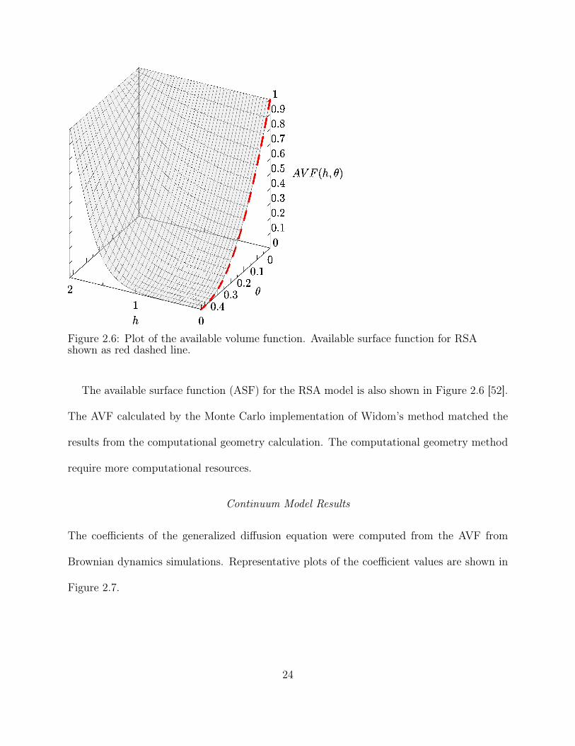
Figure 2.6: Plot of the available volume function. Available surface function for RSAshown as red dashed line.

The available surface function (ASF) for the RSA model is also shown in Figure 2.6 [52].

The AVF calculated by the Monte Carlo implementation of Widom’s method matched the

results from the computational geometry calculation. The computational geometry method

require more computational resources.

Continuum Model Results

The coefficients of the generalized diffusion equation were computed from the AVF from

Brownian dynamics simulations. Representative plots of the coefficient values are shown in

Figure 2.7.

24

(a) Coefficient k1 (b) Coefficient k2

Figure 2.7: Coefficients of the generalized diffusion equation, derived from Browniandynamics results.

The calculation of coefficient was challenging due to the presence of AV F−1 and AV F−2 in

Equation 2.9, which result in large numbers when the value of the AVF approaches zero. The

continuum model accurately reproduced the kinetics predicted by the Brownian dynamics

simulations, as shown in Figure 2.8.

Discussion

The RDFs for particle configurations generated by Brownian dynamics simulations are almost

identical to the RDF for particles generated by RSA. This agreement indicates that the

adsorption of hard spheres is a random sequential process that is essentially independent

of transport to the surface. If kinetic predictions are not required, an RSA simulation

can be used to generate surface configurations that are equivalent to results from hard-

25

0 2 4 6 8 10

t/sec

0.0

0.1

0.2

0.3

0.4

0.5θ

ContinuumBrD, ∆t = 10−5

BrD, ∆t = 10−6

BrD, ∆t = 10−7

Figure 2.8: Kinetics of adsorption predicted by Brownian dynamics simulations and thecontinuum model for φ = 0.01.

sphere Brownian dynamics simulations, with much less computational effort. Since the pair

correlation function shows that Brownian dynamics and RSA simulations produce identical

configurations of adsorbed particles, it is not surprising that the AVF for Brownian dynamics

at h = 0 is identical to the ASF for random sequential adsorption of circular disks.

The AVF shown in Figure 2.6 differs significantly from the blocking function reported

in [42], which was estimated by taking the ratio of flux at the surface to the flux expected for

a perfect adsorbing boundary. In this work the AVF was computed directly by attempting

to adsorb an additional particle onto a surface with adsorbed particles and verified with a

direct calculation using computational geometry. The method used here is more likely to

obtain an accurate result.

The kinetics of adsorption predicted by the continuum model matched the kinetics pre-

dicted by Brownian dynamics simulations when the Brownian time step was sufficiently

small. The continuum model required about one minute to run on a desktop PC, while the

Brownian dynamics simulation ran for up to several days on a high-performance cluster to

26

obtain equivalent results. The continuum model can be scaled to larger domain sizes much

more effectively than Brownian dynamic simulations, which require detecting collisions be-

tween particles. Collision detection scales as N2 using a brute-force approach, although

algorithms have been developed that produce linear scaling with N [53].

Future Applications

This work focused on the adsorption of hard spheres so that the results of the continuum

adsorption model could be rigorously validated by comparison to results from the RSA model

and the classical diffusion equation. However, the theoretical foundation of the model is di-

rectly applicable to particles with arbitrary force fields. The Widom method of obtaining the

generalized blocking function can also be directly applied to configurations of particles with

long-range “soft” interaction potentials. Brownian dynamics simulations of particles that in-

teract by means of DLVO forces have already been demonstrated [31, 32, 30]. An advantage

of Brownian dynamics is that it is straightforward to add additional forces and second-order

effects, such as hydrodynamic interactions, without changing the basic algorithm [30]. A

practical challenge to using this method for particles with long-range interactions is that

more computational resources will be required for running the Brownian dynamics simula-

tions and characterizing the chemical potential near the surface. Continuing advances in

simulation algorithms, parallelization techniques, and microprocessors will make Brownian

dynamics simulations even more useful in the near future.

27

Conclusions

The continuum model presented here reproduces the diffusion and adsorption of hard spheres

predicted by Brownian dynamics simulations, while requiring significantly reduced compu-

tational resources. Configurations of adsorbed particles from Brownian dynamics were an-

alyzed to obtain an available volume function, which extends the available surface function

into three dimensions. The available volume function was used to calculate values for the

coefficients of the generalized diffusion equation, and to validate the kinetics predicted by

the continuum model. The continuum model can be coupled to a general-purpose CFD

solver to predict transport and adsorption in practical applications such as biosensors and

models of organs. The method presented here can be extended to make a priori predictions

of protein adsorption if the particle-particle and particle-surface interaction potentials can

be characterized.

28

CHAPTER 3. MODELING THE KINETICS OF PROTEIN ADSORPTION

Introduction

The previous chapter advanced the theory of protein adsorption by developing a continuum

model that describes the adsorption of three-dimensional particles at an interface. In this

chapter, existing continuum models of protein adsorption will be used to interpret experimen-

tal measurements of the kinetics of protein adsorption on surfaces with varying properties.

Kinetic adsorption models from multiple sources will be formulated in a common mathemat-

ical framework and quantitatively compared. Computational fluid dynamics simulations will

be used to characterize transport limitations in the flow cell of a whispering gallery mode

(WGM) biosensor. The kinetic models will be fitted to experimental data from the WGM

biosensor, taking transport limitations into account, and used to test hypotheses about the

experimental results.

Alkylsilane Surface Modification

Many studies to date have focused on the adsorption of proteins to alkanethiol self-assembled

monolayers (SAMs), which are used to functionalize noble metal surfaces (typically gold).

These SAMs are convenient in that they are relatively easy to prepare, present highly ordered

monolayers with well-defined composition, and are compatible with integrated electrodes

and other sensor systems utilizing metal-coated surfaces, such as surface plasmon resonance

29

(SPR) sensors. In-depth discussions of alkanethiol SAMS are easily found in the literature

[54]. Less attention, however, has been given to alkylsilane monolayers, which are used to

functionalize glass or silica surfaces. This may be because they lack the highly ordered

packing formed by alkanethiol SAMs (resulting in less well defined surfaces), or a perceived

difficulty in the preparation of well-characterized alkylsilane surfaces. This is somewhat

unfortunate, as alkylsilanes represent a broad and useful class of compounds that are used

in an increasing variety of biomedical and biotechnological applications.

Alkylsilane monolayers are used to modify the surface chemistry of glass and silica sur-

faces to control the adhesion of proteins and cells. Laser ablation has been used to pattern

alkylsilane surfaces to create cytophobic and cytophilic regions that direct the attachment

and growth of cells [55]. (3-trimethoxysilylpropyl)diethyltriamine (DETA) is used as a cy-

tophilic cell culture substrate. 1,1,2,2-perfluorooctyltrichlorosilane (13F) is a hydrophobic

perfluorinated SAM that has been used to define cytophobic regions. More recently, teth-

ered chains of polyethylene glycol (SiPEG) have been used as cytophobic SAMs in place of

13F [56]. Surfaces modified with PEG, which is also known as oligo(ethylene glycol) (OEG)

or polyethylene oxide (PEO), have been extensively studied because of their resistance to

protein adsorption [57].

A biosensor system utilizing whispering gallery mode technology, where the active sensor

is typically a silica disk, ring, toroid, or sphere/spheroid, can provide new insights into the

adsorption behavior of biomolecules onto alkylsilane-modified surfaces. Glass and silicon

oxide surfaces are much more common than metal surfaces in cell culture applications, so

silane surface modification is of greater practical importance than thiol surface modification

for tissue engineering. To fully understand the behaviour of cells and tissue constructs, it is

30

critical to understand the underlying processes that govern the adsorption of biomolecules

to silica substrates and the alkylsilane coatings used to functionalize them.

Whispering Gallery Mode Biosensing

WGM biosensing is based on monitoring the frequency shift of an optical resonance excited

inside a dielectric resonator [58, 59]. In our implementation, near-infrared light is evanes-

cently coupled to a glass microsphere with a radius of 50-200 μm from a tapered optical

fiber, which is connected to a tunable distributed feedback (DFB) laser at one end and a

photodetector at the other. The laser and detector are used to precisely monitor changes

in the resonant wavelength of the microsphere. As proteins or other material accrete at the

surface of the microsphere, the effective radius of the sphere increases, resulting in a red shift

of the resonant wavelength that can be quantified and used to calculate the average surface

density of adsorbed material. Even with a simple experimental configuration [59] it has been

shown that a detection limit of ∼ 1 pg/mm2 can be readily achieved. This is ten times more

sensitive than an SPR biosensor and theoretical calculations predict the ultimate detection

limit of the method to be close to the single molecule level [60, 61, 62, 63]. These qualities

make WGM biosensing an ideal method for studying protein adsorption, as the dynamic

range of the method allows measurements to be performed in concentration regimes that

previously were unattainable. To date, optical resonators of this kind have been applied to a

variety of biosensing applications with great effect. In addition to the inherent sensitivity of

the method, standard CMOS technology can be applied to fabricate arrays of resonators on

silicon wafers that provide a scalable multiplex sensing capability for detecting multiple bio-

logical or chemical markers from a single sample in parallel [64, 65]. Furthermore it has been

31

shown that these measurements can be performed in complex samples such a blood plasma

and serum [66]. This provides an added level of complexity as “real-world” samples such

a plasma and serum contain a mixture of hundreds of proteins, which may non-specifically

bind to a sensor giving inaccurate readings or false positive measurements.

Fibronectin

The unique capabilities of the WGM sensor were utilized to quantify the kinetics of the

adsorption of fibronectin (FN) onto alkylsilane surfaces. Cell studies were then done to

evaluate the biological activity of the adsorbed FN [67]. Fibronectin is an important protein

in the extracellular matrix (ECM) that mediates the interaction of cells with surfaces, but its

activity has been shown to be influenced by its surface structure [68, 69]. Since the adsorption

of FN has been widely studied, the results from the WGM instrument could be compared

to an extensive amount of data. Fibronectin (FN) is a physiologically important protein in

vertebrates. It is abundant in plasma and other bodily fluids, and plays an important role in

the extracellular matrix. The structure of fibronectin is complex. The primary structure of

FN is a chain composed of three types of repeated modules. Although only one gene codes

for FN, alternative splicing of the pre-mRNA results in numerous variants in which modules

are added or deleted [70]. X-ray crystallography has been used to determine the secondary

and tertiary structure of the three types of modules. The complete FN molecule has not

been crystallized, so its secondary and tertiary structure are unknown. It is likely that the

secondary and tertiary structure are highly dependent on the local environment. In solution,

fibronectin exists as a dimer with two identical subunits linked by disulphide bonds. In the

extracellular matrix, fibronectin is assembled into a fibrillar network [71].

32

Glucose Oxidase

The WGM biosensor was also used to quantify the kinetics of adsorption of glucose oxidase

(GO) onto alkylsilane surfaces. The activity of the adsorbed enzyme was measured to provide

more information about its conformation on the surface. Glucose oxidase is an important and

useful enzyme from a technological standpoint. GO which has been adsorbed or covalently

attached to electrodes forms the basis for amperometric glucose sensors [72]. Advances in

portable blood glucose sensors have enabled diabetics to monitor and control their blood

glucose levels, minimizing the risk of complications from the disease [73]. Perhaps because

of its important role in biosensors, glucose oxidase has been thoroughly characterized. This

makes it an ideal candidate for testing and validating the accuracy of the WGM biosensor

system.

GO is a dimeric glycoprotein that is composed of two identical subunits [74]. The crystal

structure of GO from Aspergillus niger is available at the Protein Data Bank (1CF3), and

its bounding box is 6.0nm x 6.2nm x 7.7nm. Reported values for the molecular mass of GO

range from 152 kDa [75] to 186 kDa [76], depending upon the method of purification that was

used. The isoelectric point of GO is 4.2 [77]. Many previous studies have focused on the effect

of different surface chemistries on the structure and activity of adsorbed glucose oxidase [78,

79]. Atomic force microscopy (AFM) studies have been performed to determine the size and

shape of GO adsorbed on various surfaces [80, 81]. Although the immobilization of glucose

oxidase has been widely studied, only qualitative results have recently been reported for the

kinetics of adsorption [80].

33

Fitting Kinetic Models to Protein Adsorption Data

As mentioned in the previous chapter, kinetic models have been formulated as boundary

conditions for use in computational fluid dynamics (CFD) simulations of the transport and

adsorption of proteins [34, 35]. Kinetic models have also been fitted to experimental measure-

ments of adsorption kinetics. An RSA-type model with a simple approximation of transport

limitations was fitted to kinetic data from an OWLS adsorption sensor [82]. More recently,

a model of adsorption with a post-adsorption transition [83] was fitted to a comprehensive

set of kinetic data from a surface plasmon resonance sensor [69]. The concentration near

the surface was assumed to be constant. These two approaches were combined in a study in

which a Langmuir-type kinetic model coupled to a CFD simulation was fitted to experimen-

tal measurements of adsorption kinetics in microcapillaries [33]. This study was unique in

that the entire CFD model, including transport and adsorption, was included in the fitting

procedure.

Overview

A novel WGM biosensor was constructed and used to quantitatively study the kinetics of

adsorption of GO and FN at varying concentrations onto alkylsilane monolayers presenting

well-defined surface chemistries: DETA, 13F, and SiPEG. To determine the biological ac-

tivity of the adsorbed FN, neuronal and skeletal muscle cells were cultured on the modified

surfaces in a serum-free culture system [84, 85]. The kinetics of adsorption of glucose oxi-

dase were also measured on the silane monolayers and bare glass with the WGM biosensor,

and its enzymatic activity on each surface was determined with a standard assay kit. The

WGM biosensor incorporated a flow cell which minimized the effect of transport limitations

34

on protein adsorption. This, along with the inherent sensitivity of the method, allowed the

kinetics of adsorption of FN to be measured at concentrations lower than those that have

previously been reported [69]. Multiple kinetic models of protein adsorption were fitted to

the measured kinetic curves, and the resulting parameters were used to draw conclusions

about the mechanisms of adsorption. To maximize the accuracy of the fitted kinetic param-

eters, computational fluid dynamics simulations were used to quantify the limitations in the

transport of protein to the sensor surface. The results demonstrate that the combination

of WGM biosensing, CFD, and kinetic models of adsorption provides a unique capability to

quantify protein adsorption on silane-modified surfaces for the purpose of understanding the

interactions between tissues and tailored interfaces.

Methods and Materials

Experimental Methods

A whispering gallery mode sensor system was constructed as described in [86, 87]. A

schematic overview of the system is shown in Figure 3.1. After the assembly of the flow

cell, PBS solution was flowed through the tubing and flow cell until the system reached

thermal equilibrium. Protein solution at the appropriate concentration was flowed through

the system with a peristaltic pump at a volumetric flow rate of 150µl/hr. LabVIEW (Na-

tional Instruments, Austin, TX) was used to control the sweep of the laser wavelength and

acquire data. The data acquisition software tracked the location of each resonant valley in

the acquired spectrum using a peak fitting algorithm. All valleys with a FWHM (full width

at half maximum) value below a certain threshold were tracked, and the position of each

valley minimum was determined by fitting a Bessel function. The position of each resonance

35

Figure 3.1: Schematic diagram of the whispering gallery mode biosensor

over time was saved to a binary file to be analyzed later.

Data analysis software was written using the Python programming language. The binary

file created by LabVIEW for each experiment was loaded into the software and the spectral

location (nm) of each resonance was reconstructed over time from the raw data. One reso-

nance, with a continuous trace and the lowest FWHM value, was chosen for further analysis.

A linear baseline subtraction was applied to correct for baseline drift. The refractive index

of adsorbed protein (about 1.45) is similar to that of glass [88], so adsorbing proteins ef-

fectively increase the diameter of the spheroidal resonator. A method based on first order

perturbation theory [59, 63] was used to calculate the surface concentration of the adsorbed

species Γ (molecules cm−2) based on the measured change in resonant wavelength ∆λ:

∆λ

λ=

αexΓ

ε0 (n2s − n2

m)R(3.1)

36

λ is the nominal wavelength of the resonance (1310nm), ∆λ is the wavelength shift of the

resonance, ns is the refractive index of the spheroid (1.46) [89], nm is the refractive index

of the medium surrounding the sphere (1.3357) [88], αex is the excess polarizability of the

protein molecule, ε0 is the permittivity of free space and R is the radius of the spheroid.

The excess polarizability of the protein can be calculated from the refractive index increment

dn/dc:

αex = 4πε0ns2π

dn

dcm (3.2)

where m = NA/M is the mass (in grams) of a single protein molecule and M is the molar

mass. Equation 3.2 can be substituted into equation 3.1 and solved for surface concentration

to obtain

Γ =∆λ

λ

(n2s − n2

b)R

2nb dn/dc

NA

M(3.3)

The molar mass was not needed to calculate surface density ρ (g cm−2):

ρ = ΓNA

M=

∆λ

λ

(n2s − n2

b)R

2nb dn/dc(3.4)

The generally accepted value for the refractive index increment of a dilute protein solution

(0.184 cm3g−1) was used to compute the excess polarizability [59, 90]. Spheroid radii were

measured from images taken using brightfield microscopy. Two runs for each concentra-

tion were averaged for the DETA and 13F surfaces, and a single run was used for each

concentration on the SiPEG surface.

37

Surface Preparation

A single mode optical fiber with an acrylate polymer coating, 9µm core and 125µm cladding

(SMF-28e+, Corning Inc., Corning, NY) was used to fabricate the resonators [59]. The

acrylate coating was first removed using a fiber optic stripper and the stripped region was

cleaned with isopropyl alcohol (iPA) to remove any residual acrylate. The end of the stripped

fiber was then placed in the flame of a nitrous-butane Microflame torch (Azuremoon trading

company, Cordova, TN). A nitrous-butane flame was used due to the very high temperatures

needed to melt the glass and form the resonator (> 700◦C). The tip of the fiber was placed

in the flame until the glass glowed bright white and began to melt. The surface tension of

the molten glass caused it to form into a spheroidal droplet. As the tip melted, the fiber was

rotated to ensure that the resonator remained centered on the stalk of the fiber. Resonator

radii used for these studies ranged from 125µm to 175µm.

Glass resonators and glass cover slips (for control measurements) were modified with

silane surface chemistry to achieve the desired surface properties. The glass was first treated

with an oxygen plasma for 20 minutes. All silane solutions were prepared at a concentra-

tion of 0.1% (vol:vol) in distilled toluene in an MBraun glove box (Stratham, NH) under

anhydrous, low oxygen conditions. Storing and preparing solutions in this way prevented

solution phase polymerization of the silane as nascent water vapor and atmospheric oxygen

can react with the monomer. Preparation of 13F surfaces was performed in the glove box due

to the extreme reactivity of the monomer. Microspheres were immersed in the 0.1% 1,1,2,2-

perfluorooctyltrichlorosilane solution for 30 minutes. 5 minutes prior to completion of the

reaction, the beaker was removed from the glove box and placed in a chemical fume hood.

38

Both the SiPEG and DETA surface modifications were performed in a chemical fume hood.

The SiPEG coating was achieved by starting with a 0.1% solution (vol:vol) of 2-[Methoxy-

poly(ethyleneoxy)propyl]trimethoxysilane (Gelest, Tullytown, PA) and adding concentrated

HCl to create a 0.08% HCl solution (vol:vol). The resonators and cover slips were immersed

in the resultant solution for 1 hour. DETA coated substrates were immersed in a 0.1% solu-

tion (vol:vol) of (3-trimethoxysilylpropyl)diethyltriamine (Gelest) in toluene, gently heated

to 65◦C over 30 minutes and then allowed to cool for 15-20 minutes. Substrates were rinsed

three times with fresh toluene and heated again to 65◦C in fresh toluene for 30 minutes.

Upon completion of the reactions, the microspheres and cover slips were washed three times

in dry toluene and stored in a desiccator until needed. Control cover slips were analyzed by

XPS and contact angle goniometry, and the results were consistent with previously published

results [56].

Fibronectin

The kinetics of FN adsorption were measured with the WGM biosensor as described in [86].

The experiments will be briefly summarized here. Bovine plasma fibronectin in solution

(F1141, Sigma-Aldrich, St. Louis, MO) was diluted with 50mM phosphate buffered saline

(PBS) at pH 7.4. Concentrations of 10µg/ml, 5µg/ml, 1µg/ml, 0.5µg/ml and 0.25µg/ml

were used for the experiments. To determine the biological activity of the protein adsorbed

on the various silanes, cell culture experiments were performed on silane-coated cover slips

that had been treated with 1µg/ml of FN in PBS (pH 7.4). Embryonic hippocampal neurons

and skeletal myoblasts were cultured on the SiPEG, DETA, and 13F surfaces in a serum-

free culture system [84, 85]. After plating, cultures were maintained in a water-jacketed

39

incubator at 37◦C (85% relative humidity) and 5% CO2 for seven days. Phase-contrast

microscopy images were taken during the course of the culture to document the morphology

of the cells and, in the case of skeletal myoblasts, the differentiation of the cells into functional

myotubes. A live-dead assay (Invitrogen, Carlsbad, CA) was performed at day 7 to determine

the amount of living versus dead cells on the cover slips.

Skeletal muscle was dissected from the hind limb thighs of a rat fetus at embryonic day

18 (Charles River Laboratories, Wilmington, MA) as previously described [86]. Purified

myocytes were plated at a density of 500-800 cells per square millimeter onto FN-coated

cover slips. Myocytes were allowed to attach for 1 hour after which time 3 ml of culture

medium (neurobasal media containing B-27 (Invitrogen, Carlsbad, CA]), Glutamax (Invitro-

gen, Carlsbad, CA), and Penicillin/Streptavidin) was added. Culture medium was exchanged

every 4 days.

Embryonic hippocampal neurons were prepared according to a previously published pro-

tocol [86]. Rat pups at embryonic day 18 were dissected from timed pregnant rats and

the hippocampi were isolated from the embryonic brains. Isolated hippocampal neurons

were resuspended in culture medium (Neurobasal / B27 / Glutamax\u2122 / Antibiotic-

antimycotic) and plated at a density of 75 cells per square millimeter. After plating, 3 ml of

culture media was added. Half of the culture medium was changed every 3-4 days.

Glucose Oxidase

Glucose oxidase from aspergillis niger was obtained from Sigma-Aldrich (G7141, St. Louis,

MO) and diluted to 100µg/ml and 10µg/ml with PBS at pH 7.4. The kinetics of GO

adsorption were measured with the WGM biosensor using the same protocol as the FN

40

experiments. For the activity assay, glass resonators were placed in a 96-well plate and

incubated for two hours in the glucose oxidase solution. The resonators were then rinsed

three times with PBS, placed in a new 96-well plate and allowed to soak for two hours in 100µl

of PBS to remove any reversibly-bound enzyme. The Amplex Red glucose oxidase activity

assay (Invitrogen, Carlsbad, CA) was used to test the activity of the enzyme adsorbed to

the resonator. 50µl of the PBS was removed from each well and 50µl of Amplex Red

solution was added. A Synergy HT plate reader (Bio-Tek, Winooski, VT) was used read the

absorbance of each well at a wavelength of 530nm. A standard curve, created using known

concentrations of GO, was used to translate the absorbance measurements into activity units.

Analysis of Transport in the WGM Biosensor

The rate of adsorption on a surface may be limited by the rate at which the chemistry of

adsorption takes place, the rate of transport to the surface, or both. Computational fluid

dynamics was used to model the transport of protein in the flow cell of the WGM biosensor.

Before beginning, the Reynolds and Knudsen numbers were calculated confirm that flow

in the device would be entirely laminar and that conventional CFD simulation methods

were appropriate. CFD simulations were run with a CFD-ACE+ multiphysics solver (ESI

Software, Huntsville, AL) to determine the influence of transport on the adsorption of protein

on the resonator surface. For all CFD simulations, the size of the mesh and the time step

were refined until the simulation results did not change significantly. Upwind differencing

was used to approximate velocity derivatives, a 2nd order limiter was used to approximate

concentration derivatives, and the fully implicit Euler method was used for time stepping in

transient simulations. A constant-velocity boundary condition was used at the inlet, a fixed-

41

Figure 3.2: Model of the flow cell with tubing used for the first stage of CFD simulations. Aclose-up of the mesh is shown at right. The inlet tube has been truncated in these images.

pressure boundary was used at the outlet, and no-slip boundary conditions were applied on

all the surfaces.

A multi-scale approach was used to obtain high-resolution results while keeping the sim-

ulation run time reasonable. A model of the entire flow cell, including the 40 cm of tubing

between the three-way stopcock and the flow cell, was created using CFD-GEOM and dis-

cretized using a structured mesh. The model is shown in Figure 3.2. This model did not

include the resonator and waveguide, as they have a minimal effect on the overall flow in the

channel. A steady-state simulation was performed first to calculate the flow field. Transient

simulations were then performed in which the concentration at the inlet of the tubing was

suddenly increased from zero to the target concentration. The concentration of protein was

monitored at a point in the flow cell at the location of the resonator, and the simulation was

run until the concentration at this point reached the target value. It was assumed that the

low concentrations of protein used in these experiments did not affect the flow field signif-

icantly, so the transient simulations utilized the flow field from the steady-state simulation

42

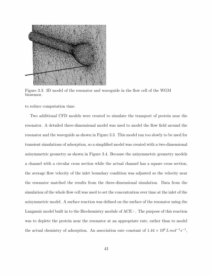
Figure 3.3: 3D model of the resonator and waveguide in the flow cell of the WGMbiosensor.

to reduce computation time.

Two additional CFD models were created to simulate the transport of protein near the

resonator. A detailed three-dimensional model was used to model the flow field around the

resonator and the waveguide as shown in Figure 3.3. This model ran too slowly to be used for

transient simulations of adsorption, so a simplified model was created with a two-dimensional

axisymmetric geometry as shown in Figure 3.4. Because the axisymmetric geometry models

a channel with a circular cross section while the actual channel has a square cross section,

the average flow velocity of the inlet boundary condition was adjusted so the velocity near

the resonator matched the results from the three-dimensional simulation. Data from the

simulation of the whole flow cell was used to set the concentration over time at the inlet of the

axisymmetric model. A surface reaction was defined on the surface of the resonator using the

Langmuir model built in to the Biochemistry module of ACE+. The purpose of this reaction

was to deplete the protein near the resonator at an appropriate rate, rather than to model

the actual chemistry of adsorption. An association rate constant of 1.44 × 106 Lmol−1s−1,

43

Figure 3.4: Overall mesh for the two-dimensional CFD model and a close-up of the meshon the resonator.

a dissociation rate constant of 8.9 × 10−4 s−1, and a maximum density of adsorption sites

of 4.4× 10−9molm−2 were used to match the maximum adsorption rate that was observed

in the experimental data for FN on DETA and 13F. A steady-state simulation was used to

establish the flow field and a transient simulation was used to determine the concentration

of protein near the surface of the resonator. The adsorption simulation mandated a fairly

small time step (on the order of 10−4 s), so it was impractical to run the simulation to

equilibrium due to the large number of time steps required. The system was simulated for

150-300 seconds (of simulated time). It was assumed that the near-surface concentration

increased linearly from the end of the CFD simulation to the target concentration.

44

Modeling the Kinetics of Protein Adsorption

It is well established that single-layer adsorption models can be stated in the general form

dθ

dt= kacΦ (θ)− kdθ (3.5)

where θ is the fraction of the surface covered by adsorbed particles, c is the concentration

of protein in solution near the surface, ka is the adsorption rate constant, and kd is the

desorption rate constant [20]. The function Φ (θ) represents the blocking effect of adsorbed

particles. For the Langmuir model, the blocking function is simply Φ (θ) = 1 − θ/θ∞.

The blocking function for the random sequential adsorption (RSA) model is not available

in analytic form. A widely used approximation for the random sequential adsorption of

spherical particles is

Φ (θ) =

(1− θ̄

)31.0− 0.812 θ̄ + 0.2335 θ̄

2+ 0.0845 θ̄

3 (3.6)

where θ̄ = θ/θ∞ [52]. Adsorption models of this form assume that proteins behave like hard

particles, with the RSA model making a further assumption that the particles pack like

spheres.

RSA-Type Model of Adsorption with Transition

Single-step adsorption models cannot adequately predict the kinetics of adsorption for many

combinations of proteins and surfaces. More complex models have been developed to account

for these experimental results. Because many surfaces cause proteins to denature upon

45

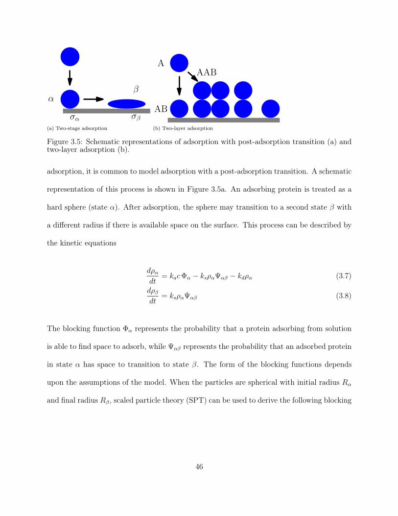
α

σα

β

σβ

(a) Two-stage adsorption

A

AB

AAB

(b) Two-layer adsorption

Figure 3.5: Schematic representations of adsorption with post-adsorption transition (a) andtwo-layer adsorption (b).

adsorption, it is common to model adsorption with a post-adsorption transition. A schematic

representation of this process is shown in Figure 3.5a. An adsorbing protein is treated as a

hard sphere (state α). After adsorption, the sphere may transition to a second state β with

a different radius if there is available space on the surface. This process can be described by

the kinetic equations

dραdt

= kacΦα − ksραΨαβ − kdρα (3.7)

dρβdt

= ksραΨαβ (3.8)

The blocking function Φα represents the probability that a protein adsorbing from solution

is able to find space to adsorb, while Ψαβ represents the probability that an adsorbed protein

in state α has space to transition to state β. The form of the blocking functions depends

upon the assumptions of the model. When the particles are spherical with initial radius Rα

and final radius Rβ, scaled particle theory (SPT) can be used to derive the following blocking

46

functions [91]:

Φα = (1− θ) exp

[−2 (ρα + Σρβ)

1− θ− ρα + ρβ + (Σ− 1)2 ραρβ

(1− θ)2

](3.9)

Ψαβ = exp

[−2 (Σ− 1) (ρα + Σρβ)

1− θ−

(Σ2 − 1)[ρα + ρβ + (Σ− 1)2 ραρβ

](1− θ)2

](3.10)

The following non-dimensional variables were defined: ρα = ραπR2α, ρβ = ρβπR

2α, θ =

ρα+Σ2ρβ, and Σ = Rβ/Rα. Since the blocking functions derived from SPT describe spherical

particles, they can be directly compared to the RSA blocking function. When ks = 0,

equations 3.7 and 3.8 reduce to equation 3.5. By setting ρβ = 0 and Σ = 1, equations 3.6

and 3.9 can be compared.

To quantitatively compare different multi-layer models, it is necessary to transform equa-

tions from different sources to use a common set of variables. The surface number densities ρi

used in equations 3.7 and 3.8 can be converted to fractional surface coverage by multiplying

by the area covered by an adsorbed particle in state i, σi, to obtain:

dθαdt

= ka σαcΦα − ksθαΨαβ − kdθα (3.11)

dθβdt

= ksΣ2θαΨαβ (3.12)

Langmuir-Type Model of Adsorption with Transition

A different model of adsorption with a post-adsorption transition has been used to fit the

adsorption kinetics of the fibronectin fragment FNIII7-10 [83, 69]. Written using the same

47

variables as equations 3.7 and 3.8, the equations that describe this model are

dραdt

= ka cAav − ks ραAav − kd ρα (3.13)

dρβdt

= ks ραAav (3.14)

where Yi is the surface density (ng/cm2) of adsorbed protein in each state. Aav is the surface

area (cm2) available for adsorption, which is given by

Aav = Atotal (1− f σ1 ρ1 − f b σ1 ρ2)

where b = σβ/σα. Since θi = σi f ρi and f = NA/M (molecules/ng), this expression can be

written Aav = Atotal (1− θ), where θ = θα + θβ. Equations 3.13 and 3.14 can be written in

terms of fractional surface coverage by multiplying both sides by σi f to obtain:

dθ1dt

= k σ1 σAtotal f c (1− θ)− sAtotal θ1 (1− θ)− r θ1 (3.15)

dθ2dt

= sAtotal b θ1 (1− θ) (3.16)

It is clear that the blocking function for this model is actually the Langmuir blocking function,

with θ∞ = 1.

Langmuir-Type Model of Two-Layer Adsorption

A two-layer adsorption model was formulated, based on the assumptions of the Langmuir

adsorption model. A schematic representation of this model is shown in Figure 3.5b. The

48

two-layer adsorption model can be represented by the chemical equations

A + Bka1,kd1←−−−→ AB

and

A + ABka2,kd2←−−−→ AAB

A represents a molecule in solution, B represents an available adsorption site, AB represents

a single molecule adsorbed on the surface, and AAB represents a “stack” of two adsorbed

molecules. The kinetics of adsorption can be modeled by a set of coupled ordinary differential

equations:

dθABdt

= ka1c (θ∞ − θAB − θAAB)− kd1θAB − ka2c θAB (3.17)

dθAABdt

= ka2c θAB − kd2 − θAAB (3.18)

θAB is the fraction of the surface covered by a single particle and θAAB is the fraction of the

surface covered by two layers of particles. θ = θAB + θAAB is the total fractional surface

coverage. Although it is straightforward to solve this set of equations analytically, the

resulting formulae are complicated, and the analysis of the solutions is beyond the scope of

this work.

Calculating the Surface Density of Active GO

Since the Langmuir and RSA models only allow protein to exist in one state, all of the

adsorbed protein must be treated as active or inactive. For the two adsorption models

49

that incorporate a post-adsorption transition, enzyme in the initial state was assumed to be

active, and enzyme in the denatured state was assumed to be inactive. For the two-layer

model, it was assumed that enzyme molecules in the upper layer prevented the substrate

solution from interacting with molecules adsorbed in the lower layer. Enzyme in the lower

layer was therefore treated as inactive. The activity of adsorbed enzyme in contact with

the surface which is not screened by an upper layer depends upon the nature of the surface.

It was assumed that hydrophilic surfaces (glass and DETA) did not induce denaturation

upon adsorption, so single-layer protein was assumed to be active. The surface density of

active enzyme was calculated ρactive = ρAB + ρAAB. For 13F (a hydrophobic surface), it was

assumed that adsorption induces denaturation and destroys the activity of the enzyme. Only

enzyme in the upper layer was considered to be active, so ρactive = ρAAB The surface densities

of active protein and total protein predicted by the models were plotted and compared to

experimental results.

Implementation of Models and Fitting to Experimental Data

A general single-layer adsorption simulation based on Equation 3.5 was implemented using

the Python programming language. Various blocking functions, such as the Langmuir and

RSA blocking functions, could be plugged into the simulation. Another simulation was

created based on equations 3.11 and 3.12 that could utilize either the Langmuir or SPT-

derived blocking function. Equations 3.15 and 3.18 were used to create a two-layer adsorption

simulation. The differential equations were solved numerically using the odeint routine

from SciPy [92]. All equations were solved in terms of fractional surface coverage to avoid

numerical difficulties that may occur when working with small floating-point numbers. For

50

comparison with experimental data, the fractional surface coverage predicted by each model

was converted to surface density (ng cm−1) using ρi = θi σ−1i f−1.

Each model was fitted to the experimental data from the WGM biosensor for glass, DETA,

13F, and SiPEG by adjusting the parameters until the best possible fit was achieved, accord-

ing to the least-squares criterion. The concentration of protein in solution near the surface

was assumed to be constant. For each surface, kinetic curves for all solution concentrations

were fitted simultaneously with a single set of parameters using the leastsq fitting routine

from SciPy, which uses a modified version of the Levenberg-Marquardt algorithm. Third-

order splines were used to interpolate the averaged experimental data to the same time points

used in the model. The quality of fit was quantified by computing the sum of squared errors

(SSE) for the total surface concentration of adsorbed protein measured by the WGM sensor

and the surface concentration predicted by the model. The SSE for each experiment was

divided by the total number of data points in the data set so that the quality of fit could be

compared between data sets with different numbers of time points.

Results

A comparison of the blocking functions of the Langmuir and RSA models is shown in Fig-

ure 3.6. The blocking function for protein in the initial state for the model derived from

scaled particle theory is also shown. It can be seen that the first-level blocking function

derived from SPT is similar but not identical to the RSA blocking function, especially at

higher values of fractional surface coverage.

The kinetics of adsorption based on the Langmuir blocking function were compared to

the kinetics modeled by the SPT blocking functions, and the results are shown in Figure 3.7.

51

0.0 0.2 0.4 0.6 0.8 1.0θ

0.0

0.2

0.4

0.6

0.8

1.0Φ

(θ)

LangmuirφFIT,3Φα

Figure 3.6: Blocking functions from the RSA model (φFIT,3) and scaled particle theory (Φα)

The parameters used for the comparison were taken from Figure 2a from [91]. Note that

0 2 4 6 8 10 12 14 16t

0.0

0.1

0.2

0.3

0.4

0.5

(a) Blocking function from scaled particle theory

0 2 4 6 8 10 12 14 16t

0.0

0.1

0.2

0.3

0.4

0.5

θαθβθ

(b) Langmuir two-stage model

Figure 3.7: Comparison of kinetics predicted by SPT blocking function (a) and Langmuirblocking function (b) for ka = 1, ks = π, kd = π, rα = 1, Σ = 1.2, and c = 1.

Figure 2a from [91] cannot be directly compared directly with Figure 3.7 in this work, because

θβ 6= ρβ.

Transport Analysis of the WGM Biosensor

The steady-state velocity magnitude predicted by the model of the whole flow cell is shown

in Figure 3.8. It can be seen that the flow field around the resonator was symmetric about

52

Figure 3.8: The magnitude of velocity predicted by CFD simulations in the vicinity of theWGM resonator.

the long axis of the resonator, with only a minor perturbation caused by the presence of

the waveguide. This configuration ensured that the shear rate was constant in the region

where the evanescent wave was excited, minimizing any shear rate effects on the adsorption

of protein from solution. These results also confirmed that the axisymmetric model was a

reasonable choice for simulating the depletion region near the surface of the resonator.

Fibronectin

The evolution of the concentration of FN in solution near the surface of the WGM resonator

over time is shown in Figure 3.9. At 10µg/ml the concentration near the surface of the

resonator required about 150 seconds to reach its final value. Figure 3.9b indicates that the

near-surface concentration takes longer to reach its final value as the bulk concentration is

decreased. Transport was not analyzed for the SiPEG surface because its low affinity for

protein was not expected to deplete protein in solution near the surface significantly. The

53

0 50 100 150 200t (sec)

0

2

4

6

8

10

µg/ml

(a) Near-surface concentration

0 50 100 150 200t (sec)

0.0

0.2

0.4

0.6

0.8

1.0

µg/ml

(b) Same data, rescaled to show lower concentrations

0.25 µg/ml0.5 µg/ml1 µg/ml5 µg/ml10 µg/ml

Figure 3.9: CFD prediction of the concentration of FN very close to the surface of theresonator.

surface density of adsorbed FN predicted by the CFD model is shown in Figure 3.10, along

with the average experimental data.

Glucose Oxidase

A similar analysis was performed for the transport of glucose oxidase in the flow cell. The

predicted concentration near the surface of the resonator with adsorption parameters for GO

on glass is shown in Figure 3.11. The results for DETA and 13F are virtually identical. To

verify that the correct kinetic constants were used in the Langmuir adsorption model, the

surface density of adsorbed protein over time predicted by the CFD simulations was plotted

along with the measured surface density. These results are shown in Figure 3.11. Transport

was not analyzed for the SiPEG surface because its low affinity for protein was not expected

to deplete protein in solution near the surface.

54

0 50 100 150 200time (s)

0

50

100

150

200

250

ng/cm

2

(a) DETA

0 50 100 150 200time (s)

0

50

100

150

200

250

ng/cm

2

(b) 13F

0.25 µg/ml0.5 µg/ml1 µg/ml5 µg/ml10 µg/ml

Figure 3.10: CFD predictions and experimental measurements of the surface density ofadsorbed FN. Thick lines indicate CFD predictions, while thin lines indicate averageexperimental data.

0 10 20 30 40 50 60t (sec)

0

20

40

60

80

100

µg/ml 10.0 µg/ml

100.0 µg/ml

Figure 3.11: CFD prediction of the concentration of GO near the surface of the resonator.

55

0 50 100 150 200t (sec)

0

20

40

60

80

100

120

ng/cm

2

(a) DETA

0 50 100 150 200t (sec)

0

20

40

60

80

100

120

ng/cm

2

(b) 13F

0 50 100 150 200t (sec)

0

20

40

60

80

100

120

ng/cm

2

(c) Glass

Exp 10.0 µg/mlCFD 10.0 µg/mlExp 100.0 µg/mlCFD 100.0 µg/ml

Figure 3.12: Surface density of adsorbed GO predicted by CFD simulation and measuredby WGM biosensor.

56

0 500 1000 1500 2000 2500 3000time (s)

0

50

100

150

200

250ng/cm

2FN on 13F

0 500 1000 1500 2000 2500 3000time (s)

0

50

100

150

200

250FN on DETA

0.25 µg/ml0.5 µg/ml1 µg/ml5 µg/ml10 µg/ml

0 500 1000 1500 2000 2500 3000time (s)

0

5

10

15

20

25

30

ng/cm

2

FN on OEG

Figure 3.13: Measured adsorption kinetics for fibronectin on 13F, DETA, and SiPEGsurfaces.

Table 3.1: Fitted parameter values for FN on DETA.

ka (cm3 ng−1 s−1) ks (s−1) kd (s−1) σα (nm2) σβ (nm2) SSE

RSA 2.05× 10−6 3.16× 10−4 182 86.1

RSA withtransition

2.37× 10−6 1.14× 10−4 2.12× 10−4 203 380 86.0

Modeling the Adsorption of Fibronectin on Silane Surfaces

The kinetics of adsorption of fibronectin on 13F, DETA, and SiPEG are shown in Figure

3.13. The kinetics predicted by the models fitted to adsorption on DETA are shown in

Figure 3.14, and the fitted parameter values are shown in Table 3.1. The kinetics predicted

by models fitted to FN adsorption on 13F are shown in Figure 3.15, and the parameter

values for the fitted models are shown in Table 3.3. The kinetics predicted by models fitted

to FN adsorption on SiPEG are shown in Figure 3.16, and the parameter values for the

57

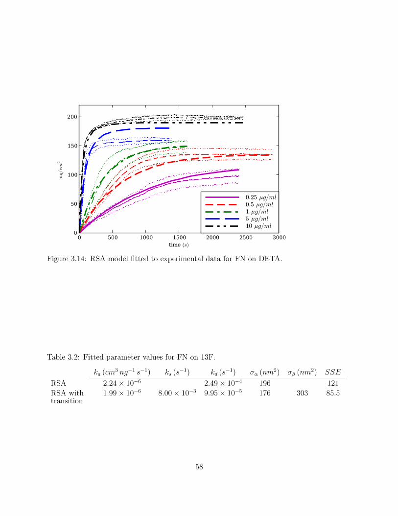
0 500 1000 1500 2000 2500 3000time (s)

0

50

100

150

200

ng/cm

2

0.25 µg/ml0.5 µg/ml1 µg/ml5 µg/ml10 µg/ml

Figure 3.14: RSA model fitted to experimental data for FN on DETA.

Table 3.2: Fitted parameter values for FN on 13F.

ka (cm3 ng−1 s−1) ks (s−1) kd (s−1) σα (nm2) σβ (nm2) SSE

RSA 2.24× 10−6 2.49× 10−4 196 121

RSA withtransition

1.99× 10−6 8.00× 10−3 9.95× 10−5 176 303 85.5

58

0 500 1000 1500 2000 2500 3000 3500time (s)

0

50

100

150

200

ng/cm

2

0.25 µg/ml0.5 µg/ml1 µg/ml5 µg/ml10 µg/ml

Figure 3.15: Adsorption model with post-adsorption transition fitted to experimental datafor FN on 13F.

Table 3.3: Parameter values fitted to FN on SiPEG.

ka (cm3 ng−1 s−1) ks (s−1) kd (s−1) σα (nm2) σβ (nm2) SSE

RSA 9.25× 10−7 7.14× 10−4 1240 2.7

RSA withtransition

1.12× 10−6 1.16× 10−2 1.04× 10−4 1240 3420 1.86

fitted models are shown in Table 3.3. Results of the cell culture experiments are shown in

Table 3.4.

Modeling the Adsorption of Glucose Oxidase on Silane Surfaces

The experimentally measured kinetic curves for glucose oxidase on glass, DETA, 13F, and

SiPEG, along with the model that achieved the best fit to each data set, are shown in

Figures 3.17, 3.18, 3.19 and 3.20, respectively. The initial rate of adsorption was highest

on the DETA and 13F surfaces and lowest on the SiPEG surface. The surface density of

adsorbed protein reached the highest saturation value on the DETA surface at 100µg/ml,

59

0 500 1000 1500 2000time (s)

0

5

10

15

20

25

30

ng/cm

2

0.5 µg/ml1 µg/ml10 µg/ml

Figure 3.16: RSA model fitted to experimental data for FN on SiPEG.

Table 3.4: Cell counts (mm−2) for embryonic hippocampal neurons and embryonic skeletalmuscle cultured on silane surfaces.

Cell Type Parameter N DETA 13F SiPEGHippocampal Live 9 212± 102 1± 3 4± 5Hippocampal Dead 9 340± 75 218± 81 265± 86

Muscle Live 4 178± 43 50± 32 0± 0Muscle Dead 4 63± 66 18± 14 111± 59Muscle Myotubes 4 35± 13 0± 0 0± 0

60

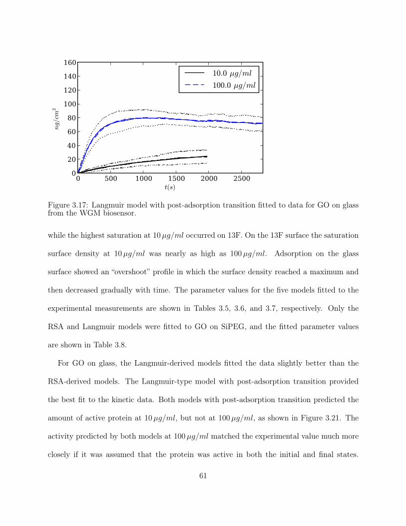
0 500 1000 1500 2000 2500t(s)

0

20

40

60

80

100

120

140

160ng/cm

2

10.0 µg/ml

100.0 µg/ml

Figure 3.17: Langmuir model with post-adsorption transition fitted to data for GO on glassfrom the WGM biosensor.

while the highest saturation at 10µg/ml occurred on 13F. On the 13F surface the saturation

surface density at 10µg/ml was nearly as high as 100µg/ml. Adsorption on the glass

surface showed an “overshoot” profile in which the surface density reached a maximum and

then decreased gradually with time. The parameter values for the five models fitted to the

experimental measurements are shown in Tables 3.5, 3.6, and 3.7, respectively. Only the

RSA and Langmuir models were fitted to GO on SiPEG, and the fitted parameter values

are shown in Table 3.8.

For GO on glass, the Langmuir-derived models fitted the data slightly better than the

RSA-derived models. The Langmuir-type model with post-adsorption transition provided

the best fit to the kinetic data. Both models with post-adsorption transition predicted the

amount of active protein at 10µg/ml, but not at 100µg/ml, as shown in Figure 3.21. The

activity predicted by both models at 100µg/ml matched the experimental value much more

closely if it was assumed that the protein was active in both the initial and final states.

61

0 500 1000 1500 2000t(s)

0

20

40

60

80

100

120

140

160

ng/cm

2 10.0 µg/ml

100.0 µg/ml

Figure 3.18: Langmuir two-layer adsorption model fitted to data for GO on DETA fromthe WGM biosensor.

0 500 1000 1500 2000 2500 3000 3500 4000t(s)

0

20

40

60

80

100

120

140

160

ng/cm

2

10.0 µg/ml

100.0 µg/ml

Figure 3.19: Langmuir model with post-adsorption transition fitted to data for GO on 13Ffrom the WGM biosensor.

62

0 500 1000 1500 2000t(s)

0

10

20

30

40

50

60

ng/cm

2

100.0 µg/ml

Figure 3.20: RSA model fitted to data for GO on SiPEG from the WGM biosensor.

Experiment

Langmuir

2-stage* RSA

2-stage

Langmuir

2-layer

0

20

40

60

80

100

120

140

160

ng/cm

2

10 µg/ml

active

total

Experiment

Langmuir

2-stage* RSA

2-stage

Langmuir

2-layer

0

20

40

60

80

100

120

140

160100 µg/ml

Figure 3.21: Experimental measurements and model predictions of GO activity on a glasssurface. The * denotes the model with the best fit to the kinetic data.

63

Experiment

Langmuir

2-stage RSA

2-stage*

Langmuir

2-layer

0

20

40

60

80

100

120

140

160

ng/cm

2

10 µg/ml

active

total

Experiment

Langmuir

2-stage RSA

2-stage*

Langmuir

2-layer

0

20

40

60

80

100

120

140

160100 µg/ml

Figure 3.22: Experimental measurements and model predictions of GO activity on a DETAsurface. The * denotes the model with the best fit to the kinetic data.

Experiment

Langmuir

2-stage RSA

2-stage

Langmuir

2-layer*

0

20

40

60

80

100

120

140

160

ng/cm

2

10 µg/ml

active

total

Experiment

Langmuir

2-stage RSA

2-stage

Langmuir

2-layer*

0

20

40

60

80

100

120

140

160100 µg/ml

Figure 3.23: Experimental measurements and model predictions of GO activity on a 13Fsurface. The * denotes the model with the best fit to the kinetic data.

64

Table 3.5: Parameters fitted to data for GO on glass.

ka (cm3 ng−1 s−1) ks (s−1) kd (s−1) σα (nm2) σβ (nm2) SSE

Langmuir 3.33× 10−8 1.15× 10−3 257 6.15Langmuirwithtransition

1.35× 10−8 1.48× 10−3 1.75× 10−3 122 414 0.73

RSA 1.16× 10−8 1.34× 10−3 80.8 7.81

RSA withtransition

3.80× 10−9 2.20× 10−3 1.99× 10−3 31.5 349 1.19

ka1 ka2 kd1 kd2 σ SSETwo layermodel

1.85× 10−8 5.46× 10−8 2.18× 10−4 4.60× 10−3 224 3.15

Table 3.6: Parameters fitted to data for GO on DETA.

ka (cm3 ng−1 s−1) ks (s−1) kd (s−1) σα (nm2) σβ (nm2) SSE

Langmuir 3.10× 10−8 1.83× 10−4 190 66.1

Langmuirwithtransition

1.15× 10−7 9.41× 10−3 3.22× 10−2 161 161 38.7

RSA 1.47× 10−8 2.15× 10−4 72.6 39.3

RSA withtransition

1.19× 10−8 0.412 2.33× 10−4 28.0 457 6.47

ka1 ka2 kd1 kd2 σ SSE

Two layermodel

1.44× 10−7 1.26× 10−8 1.19× 10−3 3.42× 10−9 363 12.7

Table 3.7: Parameters fitted to data for GO on 13F.

ka (cm3 ng−1 s−1) ks (s−1) kd (s−1) σα (nm2) σβ (nm2) SSE

Langmuir 7.20× 10−8 1.17× 10−4 247 2.45Langmuirwithtransition

5.96× 10−8 1.14× 10−2 6.74× 10−5 209 291 2.23

RSA 3.79× 10−8 3.81× 10−5 103 12.8

RSA withtransition

1.27× 10−9 0.377 9.73× 10−3 4.6 175 2.3

ka1 ka2 kd1 kd2 σ SSETwo layermodel

7.92× 10−8 7.18× 10−7 1.51× 10−4 1.28× 10−4 496 1.82

Table 3.8: Fitted parameters for GO on SiPEG.

ka (cm3 ng−1 s−1) kd (s−1) σ (nm2) SSE

Langmuir 4.06× 10−8 3.67× 10−4 684 0.81

RSA 2.18× 10−8 2.55× 10−4 482 0.73

65

For GO on DETA, the RSA-derived models fitted the data better than the Langmuir-type

models. The best fit to the kinetic curves was achieved by the RSA-type model with post-

adsorption transition. However, this model did not predict the amount of active enzyme at

10µg/ml or 100µg/ml, as shown in Figure 3.22 The two-layer model does not fit the kinetic

data quite as well, but it does predict the amount of active enzyme very well. For GO on

13F, the two-layer model and the Langmuir-type model with post-adsorption transition fitted

the kinetic data well. Although the two-layer model fitted the kinetic data slightly better,

Figure 3.23 indicates that it does not accurately predict the amount of active adsorbed

protein. The Langmuir-type model with a post-adsorption transition predicted the amount

of active protein very well.

Discussion

Although the whispering gallery mode biosensor we constructed is more sophisticated than

any WGM biosensor that has been previously reported, it is still a prototype system with

significant room for improvement. The sensitivity of the instrument could be improved by

reducing the effect of temperature on the resonant wavelengths of the spheroid. This could

be accomplished by actively stabilizing the temperature of the instrument or measuring the

temperature constantly and compensating for the temperature drift in software. Temper-

ature stabilization should eliminate the need to perform a linear baseline subtraction on

the data. The instrument could be made significantly easier to use if the resonator and

waveguide did not have to be fabricated separately and assembled by hand.

The methods used to convert the raw data (resonance wavelength over time) to final data

(adsorbed surface density over time) could also be improved. Equation 3.4 depends upon

66

several constants taken from literature, such as the refractive index of adsorbed protein and

the refractive index increment of protein in solution. The refractive index of adsorbed protein

is often taken to be constant [88]. More recent measurements have shown that the refractive

index actually depends upon the density of the adsorbed layer, which is influenced by the size

of the protein, the solvent conditions and the relaxation of the protein on the surface [90].

Refractive index increments for many proteins have been tabulated, and generally fall into

the range of 0.18−0.20 cm3g−1 [93]. However, the refractive index increment depends on the

wavelength and solvent conditions, and the infrared laser used in the WGM biosensor has a

significantly longer wavelength (1310nm) than the wavelengths at which the refractive index

increment is usually measured (∼ 600nm) [94]. The absolute surface densities reported by

the instrument could be made more accurate by measuring these values for the particular

proteins and solution conditions used in the protein adsorption experiments.

Comparison of Adsorption Models

Langmuir-type and RSA-type models are based upon different assumptions about adsorp-

tion behavior. RSA models assume that proteins act like hard spheres. Because the spheres

adsorb randomly on the surface, the surface packing is inefficient and the fractional surface

coverage reaches its maximum value around 0.547. Although it is well known that pro-

teins such as fibronectin are nothing like hard spheres, the RSA model is surprising useful

for fitting adsorption data for a wide variety of proteins. The Langmuir model makes no

assumptions about the shape of the adsorbing particles and assumes that the surface avail-

able for adsorption is a linear function of the surface coverage. Adsorption stops when a

limiting surface coverage has been reached, which may be less than 100% surface coverage

67

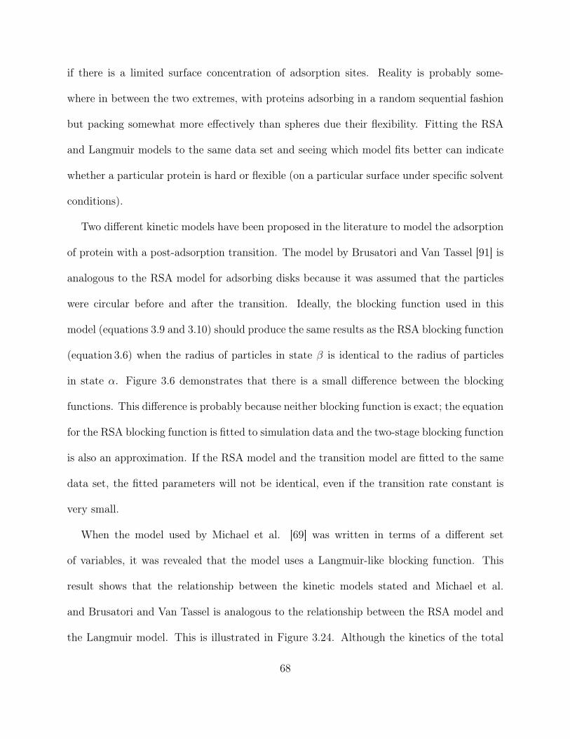
if there is a limited surface concentration of adsorption sites. Reality is probably some-

where in between the two extremes, with proteins adsorbing in a random sequential fashion

but packing somewhat more effectively than spheres due their flexibility. Fitting the RSA

and Langmuir models to the same data set and seeing which model fits better can indicate

whether a particular protein is hard or flexible (on a particular surface under specific solvent

conditions).

Two different kinetic models have been proposed in the literature to model the adsorption

of protein with a post-adsorption transition. The model by Brusatori and Van Tassel [91] is

analogous to the RSA model for adsorbing disks because it was assumed that the particles

were circular before and after the transition. Ideally, the blocking function used in this

model (equations 3.9 and 3.10) should produce the same results as the RSA blocking function

(equation 3.6) when the radius of particles in state β is identical to the radius of particles

in state α. Figure 3.6 demonstrates that there is a small difference between the blocking

functions. This difference is probably because neither blocking function is exact; the equation

for the RSA blocking function is fitted to simulation data and the two-stage blocking function

is also an approximation. If the RSA model and the transition model are fitted to the same

data set, the fitted parameters will not be identical, even if the transition rate constant is

very small.

When the model used by Michael et al. [69] was written in terms of a different set

of variables, it was revealed that the model uses a Langmuir-like blocking function. This

result shows that the relationship between the kinetic models stated and Michael et al.

and Brusatori and Van Tassel is analogous to the relationship between the RSA model and

the Langmuir model. This is illustrated in Figure 3.24. Although the kinetics of the total

68

Langmuir RSA

Michael et al. Brusatori et al.

Figure 3.24: Relationship between adsorption models.

fractional surface coverage θ are similar for both models, Figure 3.7 shows that the kinetics

of θα and θβ are very different for the two models. This difference has significant implications

for modeling experimental data if a protein in state α functions differently than a protein in

state β.

Transport Analysis

Although the flow cell was designed to minimize transport limitations, CFD simulations

showed that the near-surface concentration of fibronectin was influenced by transport limi-

tations early in the adsorption process on DETA and 13F surfaces. Initially, transport was

limited by the large amount of buffer that had to be displaced from the flow system before

the protein solution could reach the resonator at full concentration. This limitation was due

to the prototype nature of the system, and can be easily eliminated in future systems. After

the protein solution in the bulk of the flow cell reached its target concentration, the rate

of adsorption onto the resonator was high enough to deplete the fibronectin in a boundary

layer near the resonator. Because of the no-slip boundary condition at the surface and the

absence of turbulent mixing, diffusion was the only way that fibronectin could be transported

to the surface to adsorb. Fibronectin is a relatively large protein with a correspondingly low

diffusion coefficient, so its rate of diffusive transport was rather low. This type of limita-

69

tion is virtually unavoidable in microfluidic systems when the rate of adsorption is high and

the solution concentration is low. The near-surface concentration predicted by CFD was

used when fitting the adsorption models to the fibronectin data, enabling accurate kinetic

parameters to be extracted even in the presence of transport limitations.

The shape of the kinetic curves predicted by CFD simulations for the adsorption of FN

did not match the shape of the experimentally measured curves during the first minute

or so of adsorption. The experimental curves have a “sigmoidal” shape in which the rate

of adsorption increases during the first 30 seconds, while the maximum rate of adsorption

occurs at t = 0 for the predicted curves. Since the displacement of buffer from the system and

the development of the near-surface depletion layer have been modeled, another mechanism

must be hypothesized to account for this discrepancy. It is likely that a significant amount

of protein adsorbed to the silicone tubing between the reservoir and the flow cell and to the

channel walls in the flow cell. The rate of adsorption to these surfaces would be highest

when protein solution was first introduced into the system, leading to a depletion of protein

in the solution that reached the resonator. These surfaces would quickly saturate, reducing

the rate of adsorption to the tubing and allowing the protein solution to reach the resonator

at the desired concentration.

In the experiments reported here, transport limitation had much less influence on the

adsorption of glucose oxidase. GO is a smaller protein than FN, its initial rate of adsorption

is lower and the molar concentrations of GO used in these experiments were higher than the

concentrations of FN. GO reached 99% of full concentration at the resonator surface within

20 seconds, so the near-surface depletion had minimal impact on the kinetics. Constant

concentration was assumed when fitting the kinetic adsorption models to the GO data. The

70

association rate constants from fitted models (Tables 3.14-3.16 and 3.5-3.8) demonstrate that

GO has a much lower affinity for the surfaces than FN, which explains why its maximum

rate of adsorption is lower and transport limitation is much less significant.

Our modeling method was approximate in that the evolution of the near-surface concen-

tration over time was computed once, based on the estimated adsorption rate, and was not

modified during the curve-fitting procedure. A more accurate method would be to incorpo-

rate the CFD model into the fitting routine so that the near-surface concentration would be

updated as the adsorption rate changed [33]. However, this method is only practical when

the CFD simulation is simple enough to run very quickly. It was also assumed that the

near-surface concentration increased linearly from sixty seconds until the target concentra-

tion was reached. Although this probably had a slight impact on the modeled kinetics, it

was better than assuming that the concentration near the resonator remained constant.

Fibronectin Adsorption

The saturation surface concentration of FN, as measured by the WGM system, was compared

to previously published results for solution concentrations of 1µg/ml and 10µg/ml as shown

in Table 3.9. The WGM measurements compare favorably with previously published results

for a solution concentration of 10µg/ml. Although different measurement techniques and

surface preparations were used, the surface concentrations on hydrophobic and hydrophilic

surfaces were fairly similar among the various references (reference [97] being the only excep-

tion). The saturation surface concentration of FN on hydrophilic neutral surfaces measured

by the WGM sensor also indicated excellent agreement with previously published results.

However, the amount of adsorbed protein measured by the WGM system at lower concen-

71

Solution Con-centration(µg/ml)

HydrophobicSurface

HydrophilicChargedSurface

HydrophilicNeutralSurface

Ref Notes

10 200 (13F) 190 25 Thiswork

10 170 (CH3) 170 30 [95]10 160 (CH3) 30 [96]10 140 140 50 [69] FNIII7-10

fragment10 110 70 25 [97]10 ∼ 175 ∼ 175 [98] Saturation value

inferred1 135 (13F) 137 14 This

work1 20(CH3) 20 10 [95]1 20(CH3) 5 [96]1 30 25 10 [69]1 10 10 10 [97]

Table 3.9: Saturation surface density of adsorbed fibronectin (ng/cm2) from this work andprevious studies reported in the literature.

trations was significantly greater than the amount reported in previously published results

for hydrophobic and hydrophilic charged surfaces. In contrast, the surface concentration

value for a neutral hydrophobic surface was in good agreement with previous results. The

discrepancy between the WGM sensor results and the other methods at low concentrations

may be explained by differences in the measurement system, the surface chemistry, or the

adsorption process. Since the limiting surface coverages measured by the WGM sensor agree

well with other techniques for 10µg/ml and for neutral hydrophilic surfaces at 1µg/ml, the

results from the WGM sensor can be considered reliable. It is likely that if systematic errors

were inherent to the WGM method, those errors would be reflected throughout all solution

concentrations measured.

One possible interpretation of the higher saturation values measured at 1µg/ml and lower

on 13F and DETA could be the relative packing order of silane monolayers compared to alka-

72

nethiol monolayers. Alkanethiol SAMs are known to create highly ordered monolayers due to

their tight packing on highly ordered gold films [99]. Because of this tight packing only the

terminal functional groups of the alkanethiol are presented at the surface, resulting in highly

defined surface chemistries. Alkylsilane monolayers, which are formed on silica surfaces, are

less tightly packed and therefore form less ordered monolayers, which can potentially present

more than just the terminal functional group. It has been hypothesized that this may result

from interaction of electron donating groups of the silane side chain with silanol groups at

the surface resulting in reaction site-limited substrates [55]. This can lead to incomplete

monolayers that allow interaction of protein with the unreacted substrate or allow sufficient

degrees of freedom for the silane side-chains to adopt multiple conformations, creating less

ordered monolayers that can rearrange to accommodate the native protein structure. At the

high concentrations the amount of protein available to bind would swamp out these effects

but they would be present at the lower concentrations. This could explain why the differ-

ences between the silane chemistry used in this work and the alkanethiol chemistry used in

previous work [95] did not show up at 10µg/ml. Thus, this additional degree of freedom

would allow the long side chains to rearrange to accommodate greater protein interaction for

structural stabilization and higher coverage or to expose new surface sites for increased pro-

tein adsorption. This would not be possible with the tightly packed alkane thiol monolayers.

This effect could also have major consequences for protein function, as described later.

Another significant difference between the WGM measurement system and previous work

was that the protein was deposited on the WGM resonator under flow conditions and the

measurement was continued until saturation was reached, while previous measurements were

made after exposure to a static FN solution for a fixed amount of time (30-60 minutes.)

73

The combination of high-affinity surfaces and low solution concentration is conducive to

transport-limited adsorption, which could explain the discrepancy between WGM and static

experiments for hydrophobic and charged hydrophilic surfaces. In contrast, neutral hy-

drophilic surfaces have a much lower affinity for protein, so depletion of protein near the

surface would be much less of a factor, resulting in good agreement between the WGM and

static measurements.

Fibronectin on DETA and 13F

The fitted parameters of the RSA model were very similar for FN adsorption on DETA

and 13F surfaces, reflecting the similar shapes of the experimental curves. The RSA model

fitted the DETA data well, indicating that the assumptions of the RSA model were valid

for the process of adsorption on DETA. This result was confirmed by the fitting results for

the two-stage adsorption model. The mean squared error for the model with transition was

only slightly lower than the error for the fitted RSA model. We conclude that fibronectin

adsorbs on DETA with a well-defined footprint, which does not change significantly after

adsorption. This result is consistent with the well-established theory that proteins generally

experience less denaturation on a hydrophilic surface than on a hydrophobic surface [15].

The experimental results for FN on 13F showed significant deviations from the RSA model

in the saturation region, especially at higher solution concentrations. The two-stage model

allows particles to change size after adsorption, which significantly improved the fit of the

model to the data for FN on 13F. The fitted values for the association constant were quite

similar for DETA and 13F, but the transition rate constant ks for the 13F surface was an

order of magnitude larger than ks for the DETA surface. The results from the fitting process

74

indicated that FN denatured after adsorption on 13F, which had been previously postulated

for certain hydrophobic surfaces [68, 100].

Fibronectin on SiPEG

The RSA model fitted the SiPEG data well. The association rate constant for FN adsorption

on SiPEG was lower than the values for DETA and 13F while the dissociation rate constant

was higher, which is expected for a protein-resistant surface. This result is consistent with

findings that SiPEG is an electrostatically neutral surface that does not exhibit coulombic

attraction for proteins in solution. Surprisingly, the fitted radius of FN adsorbed on SiPEG

was more than twice the fitted radius of FN adsorbed on DETA or 13F. For the two-stage

model, the transition rate constant for adsorption on SiPEG was significantly higher than for

the other surfaces. The fitted pre-transition radius and post-transition radius of adsorbed

FN were also larger for SiPEG than DETA or 13F. The large radius predicted by the RSA

model and the significant transition predicted by the two-stage model seemed to indicate

that FN denatures after it adsorbs to PEG. This prediction was not consistent with the

well-known observation that proteins in contact with hydrophobic surfaces tend to dena-

ture, while proteins in contact with hydrophilic, charged surfaces tend to retain their native

conformations. However, it also may indicate that the SiPEG surface could be promoting

the denaturation of adsorbed proteins, which could explain why it is a cell-resistant surface

despite being hydrophilic.

Although the SSE of the fitted two-stage model was about 30% lower than the SSE for the

RSA model, the absolute change in SSE was relatively small, and may not be significant. It is

possible that the two extra variable parameters (transition rate constant and post-transition

75

radius) are redundant for the SiPEG surface, in which case their fitted values should not

be considered significant. It is also possible that the radius predicted by the fitting process

for SiPEG is an artifact caused by fitting the data with a model that is not well suited to

the surface chemistry. Given the assumptions of the RSA model, surface coverage can reach

saturation in only two ways: either the rate of desorption equals the rate of adsorption, or

there is no space left on the surface for another protein to adsorb. The second case may not

apply to an adsorption-resistant surface like SiPEG. However, combinations of parameters

and that fitted the initial adsorption kinetics did not predict the low saturation level of

protein observed in our experiments. One possible explanation is that FN adsorbed to a

small number of defects in the SiPEG monolayer, which could explain both the rapid initial

adsorption and the small amount of adsorbed protein when the surface is saturated. If

this were the case, a site-limited adsorption model like the Langmuir model may be better

for modeling adsorption on SiPEG. Our prototype instrument did not have the sensitivity

to perform a more thorough study of adsorption on SiPEG at low solution concentrations.

Future systems based on whispering gallery mode technology have the potential to study

the adsorption of proteins on SiPEG surfaces in greater detail, which could lead to greater

understanding as to why SiPEG resists protein adsorption.

Cell Growth and Survival on FN-Coated Alkylsilane Monolayers

Both the embryonic hippocampal neurons and myocytes showed significantly better survival

on DETA surfaces than 13F surfaces. However, measurements with the WGM biosensor

indicated that the amount of adsorbed protein measured on the 13F surfaces was compa-

rable to that of DETA, indicating that the conformation of adsorbed FN, and its function,

76

was just as important as the quantity of FN for cell survival. This is consistent with the

postulate made above that the silane monolayers are able to rearrange to accommodate more

protein and that the DETA surface, being charged and hydrophilic, could accommodate the

functional conformation of the FN so little or no denaturation would occur. Conversely, the

hydrophobic side chains of the 13F could rearrange to allow for the adsorption of more pro-

tein but would also promote the exposure of the protein’s hydrophobic core, thus denaturing

the protein and deactivating its biological activity as postulated previously for hydrophobic

surfaces [95].

Results from the skeletal myocyte culture (Table 3.4) provided further information about

the bioactivity of absorbed FN. Skeletal myocytes are precursor cells that fuse and differ-

entiate into contractile myotubes. This differentiation is mediated by, among other factors,

the interaction of the α5β1 integrin receptors on the surface of the myocytes with the cell

binding domain of the FN molecule [69]. Without this interaction, myotubes do not form.

The muscle cell culture on 13F indicated that while a significant number of cells survived,

no myotubes formed. The number of dead cells was actually less than that of SiPEG or

DETA, and the fact that so many cells survived on the 13F substrate indicates that there

was enough protein adsorbed to the surface to promote adhesion. However, the lack of my-

otube formation indicates that FN adsorbed on 13F had reduced biological activity due to

its denaturation and did not activate the α5β1 integrin signaling pathways necessary for

myotube differentiation. These proliferation and differentiation results are consistent with

previously reported results [69]. The lack of survival of cells on SiPEG surfaces can be at-

tributed to the small amount of adsorbed FN and the possibility that the protein was also

denatured.

77

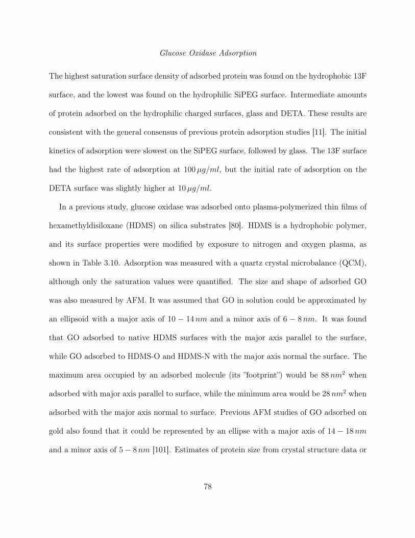
Glucose Oxidase Adsorption

The highest saturation surface density of adsorbed protein was found on the hydrophobic 13F

surface, and the lowest was found on the hydrophilic SiPEG surface. Intermediate amounts

of protein adsorbed on the hydrophilic charged surfaces, glass and DETA. These results are

consistent with the general consensus of previous protein adsorption studies [11]. The initial

kinetics of adsorption were slowest on the SiPEG surface, followed by glass. The 13F surface

had the highest rate of adsorption at 100µg/ml, but the initial rate of adsorption on the

DETA surface was slightly higher at 10µg/ml.

In a previous study, glucose oxidase was adsorbed onto plasma-polymerized thin films of

hexamethyldisiloxane (HDMS) on silica substrates [80]. HDMS is a hydrophobic polymer,

and its surface properties were modified by exposure to nitrogen and oxygen plasma, as

shown in Table 3.10. Adsorption was measured with a quartz crystal microbalance (QCM),

although only the saturation values were quantified. The size and shape of adsorbed GO

was also measured by AFM. It was assumed that GO in solution could be approximated by

an ellipsoid with a major axis of 10 − 14nm and a minor axis of 6 − 8nm. It was found

that GO adsorbed to native HDMS surfaces with the major axis parallel to the surface,

while GO adsorbed to HDMS-O and HDMS-N with the major axis normal the surface. The

maximum area occupied by an adsorbed molecule (its ”footprint”) would be 88nm2 when

adsorbed with major axis parallel to surface, while the minimum area would be 28nm2 when

adsorbed with the major axis normal to surface. Previous AFM studies of GO adsorbed on

gold also found that it could be represented by an ellipse with a major axis of 14 − 18nm

and a minor axis of 5− 8nm [101]. Estimates of protein size from crystal structure data or

78

Table 3.10: Properties of surfaces used in these experiments and similar surfaces used inprevious experiments.

Water contact angle Zeta potential (mV ) ReferenceGlass < 5◦ −25 [102, 56]DETA 49± 2◦ 10 [56, 103]13F 94± 2◦ −15 [55, 104]SiPEG 38± 2◦ [56]HDMS > 90◦ [80]HDMS-N < 50◦ 20 [80]HDMS-O Hydrophilic −40 [80]

AFM measurements on gold surfaces should be considered “order of magnitude” estimates,

since the size of proteins is heavily dependent upon their environment.

Glucose Oxidase on Glass

The Langmuir-type models fitted the kinetics of GO on glass slightly better than the RSA-

type models, and the two-stage models fitted the data better than the single-stage models.

The enzyme activity data indicated that GO adsorbed on bare glass retained about 25% of

its activity at a solution concentration of 10µg/ml. When the solution concentration was

increased to 100µg/ml, almost all of the adsorbed enzyme remained active. Both of the

two-stage models predicted the amount of active enzyme correctly at 10µg/ml, but under-

predicted the amount of active enzyme at 100µg/ml with the assumption that enzyme in

state α was active and enzyme in state β was inactive. If it was assumed that enzyme in both

states remains active, both of the two-stage models would accurately predict the amount of

active enzyme at 100µg/ml. It has been shown that some “soft” enzymes lose most of their

structure and activity when adsorbed to glass, while “hard” enzymes retain their structure

and function after adsorption [105, 106]. An alternative hypothesis is that an initial layer of

enzyme adsorbed to the surface in a highly spread-out state, resulting in a very low surface

79

density and low activity, followed by a second layer of adsorbed enzyme that retained its

activity. This could explain the low fraction of active enzyme at 10µg/ml, and the high

fraction of active enzyme at 100µg/ml. Modeling this process would require a model that

incorporated both a post-adsorption transition and multi-layer adsorption.

Glucose Oxidase on DETA

The model fits to the kinetic data for GO on DETA were not as good as the fits to the kinetic

data for GO on glass. The RSA-type model with a post-adsorption transition provided the

best fit to the kinetic data, as determined by the sum of squared error. It was assumed that

the DETA surface did not induce proteins to denature upon adsorption, and this assumption

was consistent with the data from the enzyme activity assay at 10µg/ml. When the solution

concentration was increased to 100µg/ml, approximately half of the adsorbed GO apparently

lost its activity. It is unlikely that this reduction was caused by denaturation, since adsorbed

proteins are more likely to retain their native conformation when the rate of adsorption is

higher [15]. Further, the fitted parameter values for the two-stage RSA-type model were fairly

implausible. The fitted transition rate constant was two orders of magnitude higher than the

transition rate constant for the glass surface, and the surface area occupied by a molecule

in state β was 16 times larger than a molecule in state α. A more likely hypothesis for the

50% reduction in activity is that a second layer of adsorbed enzyme formed, preventing the

substrate solution from reaching the lower layer of enzyme. The two-layer model provided the

best prediction of the amount of active adsorbed enzyme at both concentrations, although

it did not fit the kinetic data quite as well as the RSA-type two-stage model.

80

Glucose Oxidase on 13F

The kinetic data for GO on 13F was fitted well by both the Langmuir-type model with a post-

adsorption transition and the two-layer model. Although the SSE was slightly lower for the

two-layer model, the Langmuir-type model provided a much better prediction of the amount

of active adsorbed enzyme. The experimental data showed that almost none of the adsorbed

enzyme was active at a solution concentration of 10µg/ml. When the solution concentration

was increased to 100µg/ml, about 75% of the adsorbed enzyme retained its activity. GO

that adsorbs from a higher solution concentration may experience less denaturation because

it is sterically hindered from spreading out on the surface by the high density of adsorbed

enzyme molecules. Surprisingly, the fitted parameters for the Langmuir-type model with a

post-adsorption transition indicated the area occupied by a molecule in the final state was

not much larger than that of a molecule in the initial state.

Glucose Oxidase on SiPEG

Despite its sensitivity, the WGM sensor was unable to detect the adsorption of GO on an

SiPEG surface reliably at a solution concentration of 10µg/ml. At 100µg/ml, GO adsorbed

on the SiPEG surface, but at a relatively low surface density. The enzyme activity assay did

not detect any significant amount of active enzyme for either solution concentration. This

may be because the amount of activity was below the detection limit of the assay, or because

the enzyme did not retain its activity on SiPEG. It is well known that SiPEG surfaces resist

protein adsorption, but denaturation on SiPEG has not been previously reported. Further

investigation is necessary to answer this question. Both the RSA and Langmuir single-layer

models fitted this data set well.

81

Fitting Kinetic Models to Experimental Data

Fitting different models to the experimental data enabled us to test hypotheses about the

mechanisms of adsorption on various surfaces. Each model was based upon different as-

sumptions about the actual behavior of the protein at the surface. Fitting each model to

the experimental data and evaluating the quality of fit provided a quantitative methodology

to compare hypotheses and determine which assumptions were most realistic for a particu-

lar combination of protein and surface. The fitted parameter values also provided critical

information about the validity of each model. It is possible that a good fit can be achieved

with an unrealistic parameter value or combination of parameter values (such as a negative

value for a kinetic constant or radius). Therefore, it is important to understand the physical

process that is being modeled and review the fitted parameter values to ensure their valid-

ity. The least-squares fitting algorithm used in this work did not incorporate constraints

on parameter values. Many algorithms are available for constrained optimization [107, 92].

When several models fitted the data equally well, the quantitative enzyme activity data for

adsorbed glucose oxidase provided a valuable test to support or reject a particular model.

It was assumed that the kinetic constants did not vary across the limited concentration

range in this study. Therefore, a single set of parameters was fitted to multiple concentrations

for a single surface. Fitting more concentrations, while holding the number of fitted param-

eters constant, increased the possibility of finding a unique combination of parameters that

minimized the mean-squared error. A model with too many parameters can have multiple

parameter sets with equivalent optimal fits, much like an under-determined system of linear

equations can have multiple solutions. Although a lower SSE could have been achieved by fit-

82

ting data at each concentration individually, the likelihood of finding non-unique parameters

would have increased.

Finding a unique combination of parameters that provides a “best fit” to the data is

equivalent to finding a global minimum in an optimization problem. While this is not too

difficult for the basic Langmuir and RSA models (which have only three parameters each), it

becomes more challenging for the multi-stage and multi-layer models (with five parameters

each). It is easy to formulate even more complex adsorption models, but the addition of

each parameter increases the difficulty of finding a global minimum in the error function.

The danger of a very complex model with many variable parameters is that it can be fitted

to almost any data set but few useful conclusions can be drawn from the results! If models

with more parameters must be used, it will be necessary to find additional experimental

methods that can provide additional data or decrease the size of the search space. It may

also be necessary to use novel nonlinear optimization methods, such as genetic algorithms,

to optimize the fit of the model to the data.

Conclusions

The combination of simulations and experiments described in this chapter allowed protein

adsorption to be studied in a way that would not be possible with either technique by itself.

Utilization of the WGM sensor enabled, for the first time, quantitative analysis of protein

adsorption on silane monolayers, which are commonly used as substrates for cell culture.

The sensitivity of this technology can be readily enhanced by a number of methods, such as

fabricating smaller microspheres and using a laser with a shorter wavelength [62] or coating

the glass microsphere with a high-index wave-guiding layer [108]. WGM biosensors have the

83

potential to help answer difficult questions in biomaterials research. For example, PEG/OEG

monolayers are resistant to protein adsorption but have not been shown to be useful as long-

term biocompatible coatings for implants and medical devices. The field of bioengineering

would benefit from the development of a surface coating that reduces or eliminates the

immune response to a foreign body, such as an implanted medical device.

The work described here combined well-known modeling techniques in a novel way to

achieve a detailed understanding of protein adsorption on silane surfaces. Computational

fluid dynamics simulations were used to design and characterize the flow cell of the WGM

biosensor, while most experimental studies have used simple approximate models of trans-

port limitations or neglected them altogether. The results of the CFD simulations were

incorporated into the process of fitting kinetic models to fibronectin adsorption data (this

step was unnecessary for glucose oxidase.) Four existing adsorption models and one new

model were formulated in terms of the same variables and fitted to the experimental data,

and the quality of fit and fitted parameter values were compared. It is common to fit a

single model to experimental data. Fitting five models and comparing the results resulted in

a thorough and comprehensive study of protein adsorption on surfaces used for cell culture.

84

CHAPTER 4. CFD SIMULATION OF TRANSPORT IN A MICROFLUIDICBIOREACTOR

Introduction

The principles of transport and adsorption described in the previous chapters were applied to

the design of microreactors that form the liquid flow path for a functional in vitro model of an

alveolus. Alveoli are micro-scale structures in the lung that facilitate the exchange of oxygen

and carbon dioxide between the blood and inhaled air. Each alveolus is typically 200−250µm

in diameter, and the 300-480 million alveoli in the lungs of an adult human provide a total

surface area of 50−100m2 for gas exchange [109]. The alveolar membrane consists of a single

layer of epithelial cells in contact with the air and a single layer of endothelial cells that

forms a capillary for blood flow. Development of an in vitro model of the alveolus-capillary

interface would be important to biomedical science, as this barrier tissue is a point of entry

for toxins and plays a role in compromised gas exchange in disease states. A recent study

found that only 11% of the drugs that passed preclinical trials eventually became approved

for use by either U.S. or European regulatory agencies, and that the major causes of drugs

failing clinical trials were lack of efficacy and toxicity [110]. The majority of these failures

occurred in the expensive late phases of clinical trials. With the potential to overcome the

failures of traditional cell-based drug assays in predicting physiological behavior, body-on-

a-chip devices have become an increasing area of interest in pharmaceutical testing [111].

85

Body-on-a-chip devices have been created based on pharmacokinetic models in attempts to

supplement traditional cell culture methods that are not always capable of modeling the

tissue-tissue interactions that can occur when the body is exposed to pharmaceuticals [112].

Creating an in vitro model of the alveolus poses unique challenges due to the gas-liquid

environment, layers of disparate functional cell types, and the transport of nutrients, cells,

and dissolved gas species through the tissue. One lung-tissue based device was produced

out of poly(dimethyl siloxane) (PDMS) to recreate the structure, mechanics, and certain

aspects of transport that occur in lung tissue [113]. The elastomeric PDMS material used

in the device was highly permeable to both oxygen and carbon dioxide, which precluded

the ability to create physiologically relevant gas concentrations in the liquid phase of the

environment. Additionally, the high gas diffusion through the PDMS prevented measurement

of gas transport through the tissue, a fundamental function of the alveolus-capillary interface.

To overcome these limitations silicon microfluidic technology was utilized to create an in

vitro body-on-a-chip model of the lung with a long-term goal of quantifying the rate of gas

transport across the model alveolar membrane. A schematic showing the concept for the

design of the in vitro alveolus is shown in Figure 4.1.

Protein adsorption plays an important role in the microfluidic model of the alveolus. A

PDMS membrane was chosen as the substrate for culturing monolayers of epithelial and

endothelial cells because of its high permeability to oxygen and carbon dioxide. PDMS is re-

garded as a poor substrate for cell culture, so it is standard practice to treat the polymer with

an oxygen plasma and adsorb fibronectin onto the membrane prior to tissue culture [114].

Another advantage of PDMS is that it can be easily molded to create intricate shapes. This

capability will eventually be utilized to create porous membranes that will allow nutrients,

86

Figure 4.1: A schematic view of the concept for the design of the in vitro alveolus. Cellswill be cultured on the PDMS membrane in the alveolar chamber.

chemical signals and even macrophages to pass between the air and liquid sides of the mem-

brane.

Upon entering the device, the liquid flows through a conditioning chamber and exchanges

carbon dioxide and oxygen with a conditioning gas through a PDMS membrane. The con-

ditioning gas is a custom mixture of carbon dioxide and oxygen that has the same gas

composition as venous blood. The liquid then enters the alveolar chamber with the same gas

composition as venous blood. To be able to detect small changes in the rate of gas exchange

across the model alveolar membrane, the alveolar chamber was designed such that the gas

composition of the liquid reaches arterial values just before the liquid exits the chamber.

After leaving the alveolar chamber, the liquid passes through another chamber containing

dissolved-gas sensors. These sensors require several minutes to register small changes in gas

levels, so the system was designed to be operated in either continuous or stop-flow mode.

The microfluidics were designed so that a “plug” of fluid moves from the alveolar chamber

87

into the sensor chamber with relatively little mixing in the the longitudinal direction. The

residence time distribution of an ideal plug-flow system is a Dirac delta function, so the

width of the residence time distribution can be used to characterize how similar a system is

to plug flow. Each chamber must be designed so that liquid flowing through different parts

of the chamber experiences a similar residence time within the chamber. This objective is

equivalent to minimizing the width of the residence time distribution, or approximating plug

flow.

Microreactors have recently been employed for synthetic organic chemistry, nanoparticle

synthesis, and ultra-fast DNA amplification [115]. However, the combination of the no-slip

boundary condition and laminar flow in microfluidic devices produces flow patterns that

deviate substantially from the desired plug flow, presenting a challenge to the design of

continuous-flow microreactors [116]. Several innovative methods have been developed to cre-

ate plug flow in a microreactor, such as creating a multiphase flow with dispersed droplets

or “slugs” of water containing reagents in a stream of oil [117] or gas [118]. For single-phase

flows, a passive microfluidic structure known as a herringbone mixer can be added to a mi-

crofluidic channel to reduce the width of the residence time distribution to approximate plug

flow [119]. Ideally, combinations of simulation based design and experimental validation of

the results would be the best approach for successful system development. However, general

methods for minimizing the residence time distribution in a continuous-flow microreactor by

a combination of simulation and experiment have not been reported.

In experimental attempts to optimize microfluidic systems, the primary method em-

ployed for visualizing flow patterns in the devices has involved fluorescent or colored dyes

[120, 121, 122, 123]. Visualization experiments have focused mainly on the mixing of two

88

components, though this method has been used to a limited extent to measure residence

times in certain devices [124]. Both qualitative visual representations of flow and quan-

titative measurement of concentrations can be obtained using dyes, though quantitative

concentration measurements are less common. Theoretical studies have been performed to

predict the residence time distributions of various types of microfluidic structures. Analytical

models have been used to characterize the hydrodynamic dispersion in microchannels [125].

However, these methods are limited to devices with simple, well-defined geometries. Com-

putational fluid dynamics (CFD) simulations must be used to simulate practical microfluidic

devices with more complex geometries. Studies have shown that CFD simulations can pre-

dict convective and diffusive transport in microfluidic systems with a high level of accuracy

[126]. Recently, CFD simulations have been used to predict the residence time distribution

of a microfluidic mixing device by applying a pulse of a “tracer” at the inlet of the device

and monitoring the average concentration at the outlet [127]. CFD has also been used in

conjunction with a particle tracking simulation to model the residence time distribution of

a microfluidic channel containing a mixing structure [119]. Although CFD simulations have

been used to analyze the residence time distribution of microfluidic devices, the use of CFD

to optimize these devices has not been widely reported.

The field of microreactor design would benefit from a new methodology for design opti-

mization that combines experiments and simulations. This capability would be particularly

germane to biomedical engineering of new systems for drug discovery and toxicology. CFD

simulations were used as part of an iterative design process to quantify the convective and

diffusive transport of dissolved gas in the liquid side of the alveolus and optimize the design

to achieve the best possible approximation to plug flow. The flexibility of the design pro-

89

cess was demonstrated by the fabrication of an alveolar chamber that could accommodate a

standard tissue culture support and a polygonal chamber for more general applications. The

CFD predictions for different design iterations were validated with quantitative and quali-

tative experimental measurements using dye visualization. The design techniques presented

here can be utilized to optimize the performance of microreactors for any application.

Materials and Methods

Device Fabrication

Silicon was chosen as the substrate for the microfluidic device due to its impermeability to gas

and the ability to incorporate microstructures using standard microfabrication techniques,

and to allow future incorporation of other tissue compartments. A planar design was chosen

to avoid drilling or etching through the silicon substrate. Devices were fabricated using

silicon wafers with a thickness of 500µm. Wafers were liquid primed with P20 and spun

with Shipley Microposit S1818 photoresist at 3000 rpm for 60 seconds, followed by a soft

bake at 115◦C for 60 seconds on a hotplate. Exposure was performed on an ABM contact

aligner and the photoresist was developed with 726MIF developer. Silicon wafers were etched

with a Unaxis 770 deep reactive ion etcher (DRIE) to a depth of 125µm. The remaining

photoresist was stripped, and the devices were separated with a dicing saw. Devices that

incorporated all three chambers on the same chip as well as isolated chambers for each

component were fabricated and tested.

Housings were machined from acrylic plates to produce the outside portions of the mi-

crofluidic device. In the bottom section, a rectangular area was milled to approximately

0.8 mm deep into which a sheet of PDMS elastomer with nominal thickness of 0.6 mm was

90

placed. The silicon device was placed on top of the elastomer sheet so that the sheet pushed

the silicon device into the flat surface of the housing top to produce a tight seal. Inlet and

outlet holes were drilled into the housing top to direct fluid into the inlet of the silicon device

and allow the liquid to escape from the outlet. The two housing pieces each had a series

of threaded screw holes and were held together with twelve screws. The combined gasket

and silicon device thickness was larger than the depth of the rectangular recess on the bot-

tom housing piece so that the screws could be tightened to produce a seal between the top

housing piece and the silicon device.

CFD Simulation Methodology

The CFD-ACE+ suite of simulation tools was used to predict the performance of the device.

The Reynolds and Knudsen numbers were computed to ensure that flow would be entirely

laminar and that the continuum approximations inherent in CFD would be valid for the

system. CFD-GEOM was used to define the geometry and create a regular mesh throughout

the liquid volume. The velocity derivatives were approximated with upwind differencing and

a 2nd order limiter was used to approximate the derivatives for computing concentration.

A fully implicit first-order (Euler) scheme was used for time differencing and the time step

was calculated automatically using the “Auto Time Step” feature in CFD-ACE-GUI. The

minimum time step was set to 100µs. The actual time step was adjusted automatically

based upon the rate of change of the solution variables, resulting in a typical maximum

time step of 1ms. Simulation results were saved at regular time intervals. A fixed flow rate

boundary condition was used for the inlet, no-slip boundary conditions were applied at all

walls, and a fixed-pressure boundary condition was used at the outlet. The system was first

91

simulated in steady-state with pure water to determine the flow field (it was assumed that

dilute solutions of small molecules would not have a significant impact on the viscosity of

the water.) Transient simulations of gas transport were then performed, using the flow field

from the steady-state simulation to avoid re-calculating the flow field at each time step.

To characterize the residence time distribution of each design, the inlet boundary condition

introduced water saturated with carbon dioxide (mass fraction of 0.03366) at a volumetric

flow rate of 35µlmin−1, approximating a step function at the inlet of the device at t=0.

Initially, no gas was present in the water. A wall boundary condition (no gas transfer) was

used for the top wall of the chambers during the residence time simulations. The results

of this simulation protocol should also be valid for dissolved oxygen, which has a diffusion

coefficient similar to carbon dioxide (2 × 10−9m2s−1 for oxygen [128] and 1.7 × 10−9m2s−1

for carbon dioxide [129]).

Transient simulations were also performed to characterize the effectiveness of gas exchange

in the conditioning chamber and alveolar chamber. The boundary condition at the top of

each chamber was set up to model gas transport across a PDMS membrane. Since oxygen

and carbon dioxide have significantly higher solubility coefficients in PDMS than in water,

the membrane was not expected to present a barrier to gas transport. Therefore the liquid

at the upper boundary was assumed to be in equilibrium with the gas in the chamber

above the membrane. The conditioning chamber was initially filled with water with no

dissolved gas, and degassed water was introduced at the inlet. At the top of the chamber,

the concentrations of dissolved oxygen and carbon dioxide were fixed at the concentrations

found in venous blood. For the alveolar chamber, water with the gas composition of venous

blood was introduced at the inlet, and the initial condition was degassed water. Water at

92

the top of the chamber was assumed to be in equilibrium with breathing air. The transient

simulations were run until the average gas concentrations at the outlet reached steady state.

The results were visualized using CFD-VIEW. To quantify the average concentration

across the inlet or outlet channel at a specific point in time a cut plane was created across

the channel and the CFD-VIEW calculator was used to average the concentration across the

plane. The residence time distribution for the device was calculated by taking the derivative

with respect to time of the normalized concentration at the outlet.

Once the device was optimized to minimize the width of the residence time distribution for

dissolved gases in water, another set of simulations was performed to predict the transport

of dye for comparison with visualization experiments. The diffusion coefficient of Brilliant

Blue FCF dye has not been reported, so it was estimated based on known diffusion coeffi-

cients of similar dye molecules. The molar masses and diffusion coefficients of Fluorescein

(332 g mol−1), Rhodamine 6G (471 g mol−1), Congo Red (697 g mol−1), and Trypan Blue

(961 g mol−1) were plotted on a scatter plot [130, 131, 132]. A roughly linear relationship

was observed between molar mass and diffusion coefficient. Based on this relationship, the

diffusion coefficient of Brilliant Blue FCF was estimated to be approximately 2×10−10m2s−1.

Design Methodology

The chamber dimensions and internal structures were optimized by iterative computational

fluid dynamics simulations. The goal was to obtain the best possible approximation to plug

flow so that a bolus of liquid would flow through the series of chambers with minimal mixing

between the chambers. This goal was equivalent to minimizing the width of the residence

time distribution. A CFD simulation was performed for each new design and the residence

93

(a) (b) (c)

(d) (e) (f)

Figure 4.2: Progressive refinement of the design of the alveolar chamber. The diameter ofthe cell culture membrane was changed from 12mm to 6.5mm during the design process.Because the device has axial symmetry, only half of the geometry was simulated.

time distribution was calculated to evaluate that iteration. A round design was chosen for

the alveolar chamber in order to accommodate a circular cell culture membrane, such as

a Transwell insert (Corning Life Sciences). The membrane diameter was initially specified

to be 12mm but was changed to 6.5mm mid-way through the design process for reasons

unrelated to the design optimization. Once the shape and diameter of the chamber were

established, transient gas-exchange simulations were performed to establish the depth of the

chambers and the flow rate to ensure that the liquid exiting each chamber had the desired

gas concentration.

A representative sample of design iterations showing the progress of the design for the

alveolar chamber is shown in Figure 4.2. Initially, posts were added to the entrance of the

chamber to support the gas-exchange membrane and prevent fluid from passing directly

through the middle of the chamber at high velocity (Figure 4.2b). To prevent the formation

of stagnation zones around the outer edges of the chamber, the posts were changed to short

94

(a) (b) (c)

(d) (e) (f)

Figure 4.3: Progressive refinement of the design of the conditioning chamber. Because thedevice has axial symmetry, only half of the geometry was simulated.

baffles to force liquid to flow through the stagnation zones (4.2c). This was effective for

preventing stagnation near the inlet, but had little effect on stagnation near the outlet. The

baffles were then lengthened to force liquid to flow through the stagnation zones near the

outlet (4.2d,4.2e). In the final design, a small gap was added near the end of each baffle to

prevent stagnation on the channel inside of the baffle (4.2f).

The concept of the final design of the alveolar chamber can be summarized as follows.

The baffles are circular arcs which divide the incoming liquid into several streams such that

the velocity of the liquid in each stream is roughly proportional to the length of the path

it takes through the chamber. Liquid following the longest path around the perimeter of

the chamber has the same residence time as liquid traversing the shortest path through the

center of the chamber. The average flow velocity in each channel is determined by the width

of the channel and the size of the gap between the end of baffle and the center line of the

chamber. The outer baffle is just long enough to prevent a stagnation zone from forming

near the outlet of the chamber. The arc length of each baffle is as short as possible, since the

no-slip boundary condition on the baffles contributes to axial dispersion within each channel.

The starting point for the design of the conditioning chamber was a rectangle with tapering

95

inlet and outlet sections, which was based upon an existing chamber design [133]. This design

was also used for the sensor chamber and for bubble trap chambers which were included to

prevent bubbles from accumulating in the sensor chamber [134]. To allow the device to

operate in a stop-flow mode, these chambers were designed to have the same volume as the

alveolar chamber. The angle of the taper and the chamber width were adjusted to minimize

the width of the residence time distribution while maintaining a volume equal to that of the

circular chamber, as shown in Figure 4.3a and 4.3b. A staggered array of posts was then

added to distribute flow throughout the chamber and minimize stagnation zones (Figure 4.3c

through 4.3f.) The vertical spacing between posts and the number of columns of posts were

adjusted in the CFD model until the flow through the chamber was as close as possible to

plug flow. Because the chamber wall reduced the velocity of fluid flowing between the top

row of posts and the chamber wall, the spacing between the top row of posts and the chamber

wall had to be larger than the spacing between posts to avoid introducing a stagnation zone.

Dye Visualization Experiments

Blue food dye, containing Brilliant Blue FCF (FD&C Blue 1) dye, was used for visualizing

the flow of liquid through the microfluidic device. The concentration of dye in a phosphate

buffered saline (PBS) solution used in the experiments was selected based on preliminary data

of light intensity captured by the camera versus dilution of the dye solution. The solution

concentration was chosen to maximize sensitivity to changes in concentration throughout

the range of fully dilute to non-diluted from the initial concentration. For the initial solution

concentration chosen, the intensity versus concentration profile was approximately linear,

though this relationship would not hold if a higher concentration of dye was chosen. Visu-

96

alization experiments were performed by pumping the dye solution into the devices initially

containing 1X PBS with no dye and visualizing the movement of the blue dye solution in

the chambers. The dye was pumped at a rate of 35µlmin−1 using a syringe pump. The

individual chamber designs (polygonal chamber and round alveolar chamber) were tested

for dye visualization both with and without posts or baffles to evaluate the effect of the

baffle or post structures on the flow pattern. Additionally, the alveolar chamber in the final

combined device-incorporating multiple polygonal chambers and one alveolar chamber-was

tested to assess the flow pattern in the circular chamber in the practical device. The flow

visualizations in the various devices were used for comparison to the CFD predictions.

Dimensional analysis was utilized to understand how the device would perform with

dissolved gas, which has a diffusion coefficient that is roughly an order of magnitude higher

than that of the dye. The Péclet number is the dimensionless number that represents the

ratio of convective transport to diffusive transport in a fluidic system. The Péclet number in

a channel is given by Pe = LU/D, where L is the characteristic dimension of the channel, U

is the average velocity in the channel, and D is the diffusion coefficient of the solute. For a

rectangular channel, the hydraulic diameter is used as the characteristic dimension. Using the

average velocity in the channels between the chambers calculated by the CFD simulation, the

Péclet number for dissolved gas with a diffusion coefficient of 2× 10−10m2s−1 was computed

to be 770 for a volumetric flow rate of 35µlmin−1. Because the diffusion coefficient of the

dye is one order of magnitude lower than that of dissolved gas, experiments with dye were

performed with a volumetric flow rate of 3.5µlmin−1 to obtain a Péclet number comparable

to that of dissolved gas. Experiments were also performed with a flow rate of 350µlmin−1

to characterize the performance of the system over a range of two orders of magnitude.

97

Image Analysis

Images and video of the flowing liquid in the round alveolar chamber were captured using

a Hitachi KP-20a CCD microscope video camera attached to a Zeiss Stemi DV4 stereo

microscope. Because the blue dye absorbs light primarily in the red region of the visual

spectrum, the red channel of the captured images was isolated and used for image analysis

using ImageJ [135]. Video analysis was performed for flow experiments in which a solution

of dye was pumped into the device. Video was obtained at 5 frames per second from the

time dilute dye could be observed near the inlet of the chamber of interest until the entire

chamber had been filled with dye for several seconds. The average red channel intensity

was measured across a line of pixels at the inlet of the chamber and at the outlet of the

chamber for each video frame. For each frame, these average intensities for the inlet and

outlet were normalized to four points outside of the chamber unexposed to dye to account for

any variations in overall light intensity. For both the inlet and outlet, the average red channel

intensity of the first ten frames (corresponding to 0% saturation) and the last ten frames

(corresponding to 100% saturation) were computed. The average concentration across the

inlet and outlet for each frame was calculated by linearly interpolating the average intensity

between the 0% and 100% saturation intensities found from the beginning and end of the

experiment. The reported concentrations represent the average of three experiments under

the same conditions, with the curves aligned in time to the points in which the respective

inlet concentration reached 15% saturation.

98

(a) Oxygen (b) Carbon dioxide

Figure 4.4: Results of gas-exchange simulations for the alveolus and the conditioningchamber.

Results

Figure 4.4 shows the concentrations of O2 and CO2 in water at the outlet of the conditioning

chamber and alveolar chamber, for the final design of each chamber. The residence time

distributions predicted by the CFD simulations for the initial and final designs of the round

alveolar chamber and the polygonal chamber are shown in Figure 4.5a and Figure 4.5b,

respectively. Figure 4.5c shows the predicted combined residence time distribution for first

two chambers of the device (bubble trap and conditioning chamber) and for the first three

chambers of the device (bubble trap, conditioning chamber, and alveolus).

Experimental Validation of CFD Simulations

The overall layout of the device is shown in Figure 4.6a. The microfluidic device fabricated

in silicon is shown in Figure 4.6b. The silicon device in the acrylic housing is shown in

Figure 4.6c. The first chamber after the inlet is a bubble trap, followed by a chamber that will

eventually be used to condition the liquid to contain physiologically relevant concentrations

of dissolved gas. Another bubble trap is located downstream (to the right) of the alveolar

99

(a) Alveolar chamber (b) Conditioner

(c) Alveolus on full chip

Figure 4.5: Residence time distributions predicted by CFD for carbon dioxide-saturatedwater.

100

Figure 4.6: Microreactor design (a), fabricated silicon chip (b), and chip in acrylichousing (c)

chamber to prevent bubbles from accumulating in the sensor chambers, followed by two

chambers that will eventually house dissolved-gas sensors (one for CO2 and one for O2).

Four additional chip designs were fabricated (not shown) to test each chamber design in

isolation: the alveolar chamber with and without baffles and the conditioning chamber with

and without posts.

The flow pattern inside an isolated alveolar chamber with and without baffles is shown

in Figure 4.7, including both CFD results and experimental visualization. Figure 4.8 in-

dicates the amount of dye present in different locations within the isolated conditioning

chamber/bubble trap at various times. The flow patterns for the conditioning chambers

with and without the post arrangement are shown along with the flow patterns expected

from the CFD results. The visual scale of the CFD results was normalized so that pure water

was represented as white and the maximum dye concentration was black. Images from the

visualization experiments of the alveolar chamber in the combined three chamber device are

compared to the images from the isolated alveolar chamber and CFD results in Figure 4.9.

101

(a) Without baffles (b) With baffles

Figure 4.7: Visualization of the flow in the alveolus predicted by CFD (left columns) andimaged with dye (right columns)

102

(a) Without posts (b) With posts

Figure 4.8: Visualization of the flow in the conditioning chamber predicted by CFD (leftcolumns) and imaged with dye (right columns)

Figure 4.9: Visualization of the flow in the alveolar chamber in the full chip predicted byCFD (left column) and imaged with dye (right column)

103

Figure 4.10: Dye intensity at the outlet of the alveolar chamber.

Figure 4.10 indicates the dye concentration at the outlet of the alveolar chamber as

a function of time when a concentration step function was applied at the chamber inlet.

The outlet concentrations for the conditioning chamber designs, as analyzed from the video

captures, are shown in Figure 4.11, along with the concentrations expected from the CFD

results for these chambers. Figure 4.12 includes the outlet concentration of the alveolar

chamber in the three chamber design and the CFD modeling of this device. Dotted lines

indicate plus or minus one standard deviation from the experimental average, while a dashed

line indicates the concentration predicted by CFD. Figure 4.13 indicates the concentration

at the outlet of the first three chambers for flow rates equal to one tenth and ten times the

nominal flow rate.

104

Figure 4.11: Dye intensity at the outlet of the conditioning chamber.

Figure 4.12: Dye intensity at the outlet of the alveolus on the full chip.

105

Figure 4.13: Dye intensity at the outlet of the alveolar chamber in the full chip for threedifferent flow rates.

Discussion

Figure 4.4 illustrates that the chamber designs are capable of producing the desired gas

exchange characteristics. Although the steady-state concentration of carbon dioxide at the

outlet of the conditioning chamber does not quite reach the concentration found in venous

blood, this could be easily remedied by slightly changing the composition of the condition-

ing gas. The microfluidic alveolar chamber is more effective than an actual alveolus at

oxygenating the liquid and removing carbon dioxide. The rate of gas exchange across the

membrane is expected to decrease when cells are cultured on the membrane. The residence

time distributions in Figures 4.5a and 4.5b indicate that the design optimization process

clearly reduced the width of the residence time distribution for each chamber, improving the

approximation to plug flow. The residence time distribution of the round chamber without

baffles exhibited a long “tail” which was caused by the stagnation zones that formed near

106

the outlet of the chamber (Figure 4.7a). The addition of baffles forced liquid from the inlet

to flow around the outer perimeter of the chamber, greatly reducing these stagnation zones

and suppressing the “tail” of the residence time distribution. The residence time distribution

of the polygonal chamber without posts was narrower than the residence time distribution

of the round chamber without baffles. Without the constraint imposed by the circular tissue

culture membrane, the shape of the polygonal chamber could be optimized for plug-like flow

without additional structures. However, the addition of posts further narrowed the residence

time distribution. Figure 4.5c demonstrates that each successive chamber further widens the

residence time distribution so that a plug of fluid becomes more disperse as it progresses

through the device.

Dye Visualization Experiments

The experimental flow patterns confirmed the CFD predictions that introducing baffles into

the alveolar chamber would reduce stagnation zones to produce a more plug-flow like flow

pattern. At early time points, the baffles prevented a stream of dyed liquid from speeding

toward the outlet along the center line of the chamber, as shown in time points 3.5 s and

6.5 s. Especially at the later time points, the baffles reduced liquid stagnation near the outer

walls of the chamber. Stagnation zones in the alveolar chamber without baffles were clearly

visible at 11.5 s, and stagnant liquid remained at 16.5 s immediately adjacent to the walls.

In contrast, the liquid near the walls of the alveolar chamber with baffles was much more

uniform in concentration at 11.5 s, and the entire chamber had a nearly uniform concentration

at 16.5 s. The baffle design clearly improved the flow patterns in the round alveolar chamber,

though further improvements may be possible. The streaks of higher and lower concentration

107

liquid, which are prominent at 6.5 s, indicated that the flow pattern on the exit side of the

baffles was not completely uniform. It should be noted that the chambers were optimized for

the transport of gases that have diffusion coefficients an order of magnitude higher than the

diffusion coefficient of the dye used to visualize the flow patterns. Therefore, the stagnation

zones observed in the dye injection experiments are likely to be much smaller when dissolved

gas is used in place of dye.

The dye visualization of the flow patterns in the isolated conditioning chamber (Figure 4.8)

confirmed that the post layout improves the uniformity of the flow pattern in the conditioner,

like the baffles improved the flow pattern in the alveolar chamber. Specifically, at 6.5 s

and 9.5 s after the introduction of dye into the inlet the condition chamber without posts

exhibited large regions of stagnant liquid near the chamber walls, represented by lighter

color. In contrast, the chamber with posts did not experience these stagnant zones. The

CFD simulation predicted that the chamber without posts should be nearly completely

filled with dyed liquid by 6.5 s, while experiments showed that filling the chamber required

somewhat more time.

In Figure 4.9, the flow pattern for the liquid in the alveolus of the full device followed

the CFD results as well as matched the trends of the isolated alveolar chamber with baffles.

The dispersion of dye in the inlet of the alveolus due to the previous two chambers can be

observed in Figure 4.9. Because of the non-uniform concentration of dye across the inlet,

the alveolar chamber in the full device requires more time to reach a uniform concentration

compared to the single alveolar chamber. This trend can also be seen in the images from

the CFD simulation.

The images of the flow patterns (Figures 4.7-4.9) include information about the distribu-

108

tion of the outlet concentrations over the width of the chambers. In the chambers without

posts or baffles, there was variation in concentration across the width of the outlet before

full saturation was reached. The liquid near the walls had a lower concentration of dye than

the liquid in the center of the channel, due to the laminar flow within the chamber and the

channels. In both Figures 4.7 and 4.8, the posts or baffles greatly reduced this variation

across the channel width, indicating more plug-like flow.

The results from the quantitative evaluation of the outlet profiles in the isolated alveolar

chamber (Figure 4.10) further confirmed the results from the CFD simulation. In both the

CFD and in the experimental visualization, the start of the rise in concentration of the

liquid at the outlet was delayed by the presence of the baffles. Experimentally, the outlet

concentrations reached saturation at approximately the same time with and without baffles.

The delay in the onset of the increase in outlet concentration coupled with the fact that

the two outlets reached saturation at nearly the same time indicated that the liquid in the

alveolar chamber with baffles exhibited a narrower distribution of residence times.

The concentration profiles for the conditioning chambers with and without posts (Figure

4.11) reinforced the conclusion that the post layout improved the flow patterns to produce

more plug-like flow. The outlet concentrations in both chambers began to rise at approx-

imately the same time, but the two profiles began to deviate at approximately the half-

saturation point. In this chamber, the post layout improved the flow pattern by reducing

the stagnation zones, creating a steeper concentration profile at the outlet. Toward the

later times, the outlet concentration profile for the chamber without posts was delayed by

approximately 3 seconds relative to the profile of the chamber with posts.

The concentration profile at the outlet of the alveolar chamber in the full device (Figure

109

4.12) was actually steeper than the CFD results, indicating a narrower residence time distri-

bution within the entire chip than was predicted. The inlet concentration for the alveolus was

influenced by the previous two chambers, so the inlet concentration for the alveolar chamber

was not a step function for either the CFD or the experimental results. The influence of all

three chambers on the flow pattern was incorporated into both the CFD and experimental

results for the three-chamber design. The fact that the experimental concentration profile

at the outlet of the three-chamber design was only slightly shifted from the isolated alveolar

chamber indicates the entire design was quite effective at approximating plug flow.

The full device was imaged and the concentrations at the outlet of the alveolar chamber

were analyzed using flow rates covering three orders of magnitude to vary the ratio of con-

vective to diffusive mass transfer (i.e. different Péclet numbers) (Figure 4.13). As expected,

faster flow rates produced less steep concentration profiles in the normalized time scale, since

the higher convective transport rates limited the amount of diffusion that occurred during

the normalized time period. The slowest flow rate (3.5µlmin−1) simulates the outlet concen-

tration profile that would be produced using dissolved CO2 (with approximately one order

of magnitude higher diffusion coefficient than dye) at a flow rate of 35µlmin−1, since the

ratio of convective transfer to diffusive transfer is about the same for both conditions. This

condition (CO2 dissolved in a liquid flowing at 35µlmin−1) is appropriate for a lung-on-a-

chip device of similar geometry. Thus, the outlet saturation profiles for different flow rates

can be used to estimate the profiles that would be produced for other diffusion coefficients.

When comparing the original designs to the optimized designs, the improvements shown

by the experimental measurements closely matched the improvements predicted by the sim-

ulations. These results demonstrated that the CFD-based design process was effective at

110

reducing the number of experimental iterations required. The slight deviation of the simula-

tion results from the experimental results was likely due to differences in the injection of dye

at the inlet. The inlet concentration was modeled as a step function in the CFD simulations.

In the experiments, the concentration at the inlet of the chamber was not a perfect step

function because the dye was injected through a channel in the device housing which was

not included in the CFD model. In the functional lung device the conditioning chamber

will fix the concentration of dissolved gas in the liquid before it enters the alveolus, so any

dispersion introduced by the channel before the conditioning chamber will not be significant.

Conclusions

The microfluidic design presented here is a major step towards a complete in vitro model of

the alveolus. A novel design for a round chamber was developed that minimized stagnation

and functioned like a plug flow reactor despite the inherent disadvantage of the round shape.

This design could be used for any microfluidic chamber that needs to accommodate a circular

cell culture membrane. The design of the conditioning chamber shows that even better

approximations to plug flow can be achieved if the overall shape of the chamber can be

optimized. The design process, including both iterative CFD simulations and experimental

validation, can be used to optimize the design of any microreactor. Using CFD to simulate

and evaluate design iterations instead of fabricating a prototype for each iteration greatly

reduced the cost of the project and the time required to achieve the design goals.

111

CHAPTER 5. GENERAL DISCUSSION

Modeling and simulation were used to enable advances in nano-scale surface science and bio-

engineering that would have been difficult, time-consuming or impossible with experimental

methods alone. Similarly, modeling and simulation is of limited utility unless quantitative ex-

periments can be performed to inspire new hypotheses and validate the results of simulations.

Chapter 2 described the derivation of a new continuum model of hard-sphere adsorption that

allows the results of mesoscale Brownian dynamics simulations to be incorporated into con-

tinuum CFD simulations of practical devices. Although the work in this chapter was purely

theoretical, careful steps were taken to validate the Brownian dynamics simulation and the

continuum CFD simulation. The results of each simulation were compared against known

analytical results for well-defined test cases, and the results of the two simulations were

compared against one another. This chapter also illustrated the use of experimental controls

in simulation work, by checking the effect of simulation parameters such as the size of the

time step and simulation domain to ensure that artifacts are not present in the simulation

results. This multi-scale adsorption model is a step towards developing simulation tools that

can make accurate a priori predictions of protein adsorption in microfluidic lab-on-a-chip

devices.

The close coupling of experiments and simulations was continued in Chapter 3, which

112

began with a description of a WGM biosensor to study the kinetics of protein adsorption

on functionalized glass surfaces relevant for tissue culture. The biosensor does not require

any specialized equipment, and the device components (DFB laser, photodetector, optical

fiber, and simple microfluidics) are inexpensive compared to commercial systems and can be

readily assembled in any laboratory environment. Despite its simplicity, the sensitivity of

the setup rivals that of a state-of-the art surface plasmon resonance sensor (∼ 1 pg/mm2),

with the additional advantage that silica microspheres can be easily fabricated and conve-

niently modified with various silane surface coatings by exploiting established silanol surface

chemistries. This is an alternative to other methods, such as SPR, that require coating the

sensor with gold and are mostly limited to surface modification with thiols.

The WGM sensor allowed for the first time the detailed kinetic analysis of protein adsorp-

tion on silane monolayers and enabled some explanation of the differences between silane and

thiol surface modifications. The WGM sensor was used to obtain the most comprehensive

set of kinetic data that has been reported for the adsorption of fibronectin at low solution

concentrations, and the first quantitative measurement of the kinetics of glucose oxidase ad-

sorption on silane surfaces. CFD was used in the design of the flow cell, resulting in a sensor

system which predominantly measures the kinetics of adsorption rather than the kinetics

of transport the sensor. In the case of fibronectin adsorption, CFD analysis of transport

limitations in the flow cell allowed accurate kinetic parameters to be extracted from the

data set in the presence of transport limitations. Measuring adsorption kinetics at multiple

concentrations allowed a single set of kinetic constants to be fitted to multiple curves, which

increased the likelihood of obtaining a unique set of fitted parameters. Fitting multiple mod-

els to each data set and evaluating the quality of the fit allowed various hypotheses about

113

the mechanisms of adsorption to be tested. The use of modeling and simulation greatly

enhanced the conclusions that could be drawn from a set of experiments.

The results of the WGM biosensor measurements, model fitting and the cell culture ex-

periments indicate that similar amounts of FN adsorb on hydrophobic surfaces and charged

hydrophilic surfaces. When combined with antibody data from other studies, our data sup-

ports the conclusion that FN denatures after adsorption on hydrophobic surfaces, leading to

a loss of biological activity. Modeling the adsorption of GO indicated that the mechanism

of adsorption strongly depends on the surface chemistry of the adsorbing surface. One of

the most important goals in biomaterials research is to discover surfaces that resist pro-

tein adsorption. Surfaces similar to SiPEG (OEG-thiols) have been shown to be the most

protein-resistant class of surfaces [136], yet GO and FN both adsorb on SiPEG in small quan-

tities and the mechanism of protein resistance remains unknown. Models fitted to protein

adsorption on SiPEG seem to indicate that this surface may actually induce denaturation

in adsorbed proteins. The evidence presented here is tantalizing but insufficient to draw

definitive conclusions. Further improvements to the sensitivity of WGM biosensors will help

answer this and other difficult questions in biomaterials research.

The relevance of transport modeling in the design of biomicrofluidic devices was demon-

strated in Chapter 4, which presented the design optimization process for an in vitro alveolus.

Because of laminar flow and the no-slip boundary condition, transport in the original design

was not at all “plug-like,” with substantial stagnation zones in each chamber. Microfluidic

structures were added to each chamber to minimize the stagnation zones and enable a plug

of fluid to move from one chamber to the next with minimal dispersion. The results from

the full device demonstrate that the two types of chamber can be used as building blocks

114

for devices with multiple chambers. While each chamber contributes to the widening of the

residence time distribution, the optimized post and baffle designs can effectively be used

to improve overall flow patterns in a multitude of devices of similar geometry. The use of

CFD simulations enabled the optimization of the device by allowing many design iterations

to be performed without the expense and delay of fabricating a prototype at each iteration.

The CFD simulations were validated qualitatively and quantitatively with dye visualiza-

tion experiments in prototype devices. The validation protocol required only food dye and

an optical microscope with a camera-tools which are available in almost every laboratory.

This project demonstrates that simulation tools that can quantitatively predict transport

and protein adsorption will enable the rational design of microfluidic devices for biomedical

applications.

The in vitro alveolus also demonstrates the importance of quantitative protein adsorption

data. Although it is well known that PDMS must be modified before use as a cell culture

substrate, the modification protocols currently in use are empirically derived. This project

would benefit greatly from a deeper understanding of how proteins and cells interact with

PDMS. Silicone is typically treated with oxygen plasma to make it hydrophilic, and some-

times protein is adsorbed on it, before plating cells. Based on the fibronectin experiments

reported here, it can be hypothesized that FN adsorbed on hydrophilic PDMS retains a bio-

logically active conformation, while FN adsorbed on untreated hydrophobic PDMS may not

be biologically active. Whispering gallery mode technology can easily be applied to study the

adsorption of extracellular matrix proteins on PDMS. High-Q WGM resonators made out of

PDMS have already been demonstrated [137]. Because PDMS is easy to mold, it may also

be possible to integrate the leaky waveguide and resonator into one monolithic device that

115

can be mass-produced, eliminating the time-consuming and tedious task of flame-drawing a

waveguide and securing it into the flow cell with silicone adhesive. The combination of quan-

titative measurements and modeling and simulation will enable new advances in biomedical

science.

116

LIST OF REFERENCES

[1] G. M. Whitesides, “The origins and the future of microfluidics,” Nature, vol. 442,

no. 7101, pp. 368–373, 2006.

[2] K. V. Sharp, R. J. Adrian, J. G. Santiago, and J. I. Molho, The MEMS Handbook,

ch. 6. CRC Press, 2002.

[3] N.-T. Nguyen and Z. Wu, “Micromixers-a review,” Journal of Micromechanics and

Microengineering, vol. 15, no. 2, p. R1, 2005.

[4] C. Yi, C.-W. Li, S. Ji, and M. Yang, “Microfluidics technology for manipulation and

analysis of biological cells,” Analytica Chimica Acta, vol. 560, no. 1-2, pp. 1 – 23, 2006.

[5] D. N. Breslauer, P. J. Lee, and L. P. Lee, “Microfluidics-based systems biology,” Mol.

BioSyst., vol. 2, pp. 97–112, 2006.

[6] L. M. Borland, S. Kottegoda, K. S. Phillips, and N. L. Allbritton, “Chemical analysis of

single cells,” Annual Review of Analytical Chemistry, vol. 1, no. 1, pp. 191–227, 2008.

[7] T. D. Chung and H. C. Kim, “Recent advances in miniaturized microfluidic flow cy-

tometry for clinical use,” ELECTROPHORESIS, vol. 28, no. 24, pp. 4511–4520, 2007.

[8] S. K. Sia and L. J. Kricka, “Microfluidics and point-of-care testing,” Lab Chip, vol. 8,

pp. 1982–1983, 2008.

[9] R. Fox, A. McDonald, and P. Pritchard, Introduction to Fluid Mechanics. John Wiley,

117

2006.

[10] G. M. Walker, H. C. Zeringue, and D. J. Beebe, “Microenvironment design considera-

tions for cellular scale studies,” Lab Chip, vol. 4, pp. 91–97, 2004.

[11] M. Rabe, D. Verdes, and S. Seeger, “Understanding protein adsorption phenomena at

solid surfaces,” Advances in Colloid and Interface Science, vol. 162, pp. 87–106, 2010.

[12] G. Cheng, Z. Zhang, S. Chen, J. D. Bryers, and S. Jiang, “Inhibition of bacterial

adhesion and biofilm formation on zwitterionic surfaces,” Biomaterials, vol. 28, no. 29,

pp. 4192 – 4199, 2007.

[13] S. Sun, Y. Yue, X. Huang, and D. Meng, “Protein adsorption on blood-contact mem-

branes,” Journal of Membrane Science, vol. 222, no. 1-2, pp. 3 – 18, 2003.

[14] P. Roach, D. Eglin, K. Rohde, and C. Perry, “Modern biomaterials: a review—bulk

properties and implications of surface modifications,” Journal of Materials Science:

Materials in Medicine, vol. 18, no. 7, pp. 1263–1277, 2007.

[15] R. Latour, “Biomaterials: Protein-surface interactions,” in Encyclopedia of Biomateri-

als and Biomedical Engineering (G. Wnek and F. Bowling, eds.), pp. 1–15, London:

Taylor & Francis, 2005.

[16] J. Ramsden, D. Allen, D. Stephenson, J. Alcock, G. Peggs, G. Fuller, and G. Goch,

“The design and manufacture of biomedical surfaces,” CIRP Annals - Manufacturing

Technology, vol. 56, no. 2, pp. 687 – 711, 2007.

[17] J. C. K. Lai, M. P. Schoen, A. P. Gracia, D. S. Naidu, and S. W. Leung, “Prosthetic

devices: Challenges and implications of robotic implants and biological interfaces,”

Proceedings of the Institution of Mechanical Engineers, Part H: Journal of Engineering

in Medicine, vol. 221, no. 2, pp. 173–183, 2007.

118

[18] K. Wilson, S. J. Stuart, A. García, and J. Robert A. Latour, “A molecular modeling

study of the effect of surface chemistry on the adsorption of a fibronectin fragment

spanning the 7-10th type iii repeats,” Journal of Biomedical Materials Research Part

A, vol. 69A, no. 4, pp. 686–698, 2004.

[19] D. Axelrod, N. L. Thompson, and T. P. Burghardt, “Total internal inflection fluorescent

microscopy,” Journal of Microscopy, vol. 129, pp. 19–28, 1983.

[20] J. D. Andrade and V. Hlady, “Protein adsorption and materials compatibility: A tuto-

rial review and suggested hypotheses,” Advances in Polymer Science, vol. 79, pp. 1–63,

1986.

[21] R. Kurrat, M. Textor, J. J. Ramsden, P. Böni, and N. D. Spencer, “Instrumental im-

provements in optical waveguide light mode spectroscopy for the study of biomolecule

adsorption,” vol. 68, no. 5, pp. 2172–2176, 1997.

[22] M. Mrksich, G. B. Sigal, and G. M. Whitesides, “Surface plasmon resonance permits in

situ measurement of protein adsorption on self-assembled monolayers of alkanethiolates

on golde,” Langmuir, vol. 11, no. 11, pp. 4383–4385, 1995.

[23] J. J. Gray, “The interaction of proteins with solid surfaces,” Current Opinion in Struc-

tural Biology, vol. 14, pp. 110–115, 2004.

[24] M. Agashe, V. Raut, S. J. Stuart, and R. A. Latour, “Molecular simulation to char-

acterize the adsorption behavior of a fibrinogen γ-chain fragment,” Langmuir, vol. 21,

no. 3, pp. 1103–1117, 2005. PMID: 15667197.

[25] G. Raffaini and F. Ganazzoli, “Protein adsorption on a hydrophobic surface: A molec-

ular dynamics study of lysozyme on graphite,” Langmuir, vol. 26, no. 8, pp. 5679–5689,

2010. PMID: 20041676.

119

[26] R. O. Dror, M. O. Jensen, D. W. Borhani, and D. E. Shaw, “Exploring atomic reso-

lution physiology on a femtosecond to millisecond timescale using molecular dynamics

simulations,” The Journal of General Physiology, vol. 135, pp. 555–562, June 1, 2010

2010.

[27] D. Evans and H. Wennerström, The colloidal domain: where physics, chemistry, biol-

ogy, and technology meet. Advances in interfacial engineering series, VCH Publishers,

1994.

[28] C. M. Roth and A. M. Lenhoff, “Electrostatic and van der waals contributions to

protein adsorption: Computation of equilibrium constants,” Langmuir, vol. 9, pp. 962–

962, 1993.

[29] C. M. Roth and A. M. Lenhoff, “Electrostatic and van der waals contributions to protein

adsorption: Comparison of theory and experiment,” Langmuir, vol. 11, pp. 3500–3509,

1995.

[30] H. N. Unni and C. Yang, “Brownian dynamics simulation and experimental study of

colloidal particle deposition in a microchannel flow,” Journal of Colloid and Interface

Science, vol. 291, no. 1, pp. 28–36, 2005.

[31] R. V. Magan and R. Sureshkumar, “Multiscale-linking simulation of irreversible col-

loidal deposition in the presence of dlvo interactions,” Journal of Colloid and Interface

Science, vol. 297, no. 2, pp. 389–406, 2006.

[32] A. Quinn, H. Mantz, K. Jacobs, M. Bellion, and L. Santen, “Protein adsorption kinetics

in different surface potentials,” EPL (Europhysics Letters), p. 56003, 2008.

[33] J. Jenkins, B. Prabhakarpandian, K. Lenghaus, J. Hickman, and S. Sundaram,

“Fluidics-resolved estimation of protein adsorption kinetics in a biomicrofluidic sys-

120

tem,” Analytical Biochemistry, vol. 331, pp. 207–215, 2004.

[34] R. W. Glaser, “Antigen-antibody binding and mass transport by convection and dif-

fusion to a surface: A two-dimensional computer model of binding and dissociation

kinetics,” Analytical Biochemistry, vol. 213, no. 1, pp. 152–161, 1993.

[35] D. A. Edwards, “Estimating rate constants in a convection-diffusion system with a

boundary reaction,” IMA Journal of Applied Mathematics, vol. 63, pp. 89–112, 1999.

[36] J. Talbot, G. Tarjus, P. V. Tassel, and P. Viot, “From car parking to protein ad-

sorption: an overview of sequential adsorption processes,” Colloids and Surfaces A:

Physicochemical and Engineering Aspects, vol. 165, no. 1-3, pp. 287 – 324, 2000.

[37] Z. Adamczyk, B. Senger, J.-C. Voegel, and P. Schaaf, “Irreversible adsorp-

tion/deposition kinetics: A generalized approach,” Journal of Chemical Physics,

vol. 110, no. 6, pp. 3118–3128, 1999.

[38] Z. Adamczyk, “Kinetics of diffusion-controlled adsorption of colloid particles and pro-

teins,” Journal of Colloid and Interface Science, vol. 229, no. 2, pp. 477–489, 2000.

[39] Z. Adamczyk and P. Weroński, “Application of the dlvo theory for particle deposition

problems,” Advances in Colloid and Interface Science, vol. 83, no. 1-3, pp. 137–226,

1999.

[40] S. de Groot and P. Mazur, Non-equilibrium thermodynamics. Dover Books on Physics,

Dover Publications, 1984.

[41] M. Elimelech, J. Gregory, X. Jia, and R. Williams, Particle Deposition and Aggregation:

Measurement, Modelling and Simulation. Butterworth-Heinemann, 1998.

[42] R. V. Magan, “A multiscale-linking algorithm for the simulation of irreversible deposi-

tion,” Multiscale Model. Simul., vol. 2, no. 3, p. 475, 2004.

121

[43] T. E. Oliphant, Guide to NumPy. Provo, UT: Trelgol Publishing, 2006.

[44] T. E. Oliphant, “Python for scientific computing,” Computing in Science & Engineer-

ing, vol. 9, no. 3, pp. 10–20, 2007.

[45] E. Gabriel, G. E. Fagg, G. Bosilca, T. Angskun, J. J. Dongarra, J. M. Squyres, V. Sa-

hay, P. Kambadur, B. Barrett, A. Lumsdaine, R. H. Castain, D. J. Daniel, R. L.

Graham, and T. S. Woodall, “Open MPI: Goals, concept, and design of a next gener-

ation MPI implementation,” in Proceedings, 11th European PVM/MPI Users’ Group

Meeting, (Budapest, Hungary), pp. 97–104, September 2004.

[46] F. Alted, I. Vilata, et al., “Pytables: Hierarchical datasets in python,” 2002-.

[47] The HDF Group, “Hierarchical data format version 5,” 2000-.

[48] B. Widom, “Some topics in the theory of fluids,” Journal of Chemical Physics, vol. 39,

no. 11, p. 2808, 1963.

[49] R. P. A. Dullens, D. G. A. L. Aarts, W. K. Kegel, and H. N. W. Lekkerkerker,

“The widom insertion method and ordering in small hard-sphere systems,” Molecu-

lar Physics, vol. 103, no. 21-23, pp. 3195–3200, December.

[50] “Cgal, Computational Geometry Algorithms Library.” http://www.cgal.org.

[51] S. Patankar, Numerical heat transfer and fluid flow. Taylor & Francis, 1980.

[52] P. Schaaf and J. Talbot, “Surface exclusion effects in adsorption processes,” The Journal

of Chemical Physics, vol. 91, p. 4401, 1989.

[53] W. R. Taylor and Z. Katsimitsoulia, “A soft collision detection algorithm for simple

brownian dynamics,” Computational Biology and Chemistry, vol. 34, no. 1, pp. 1 – 10,

2010.

[54] J. C. Love, L. A. Estroff, J. K. Kriebel, R. G. Nuzzo, and G. M. Whitesides, “Self-

122

assembled monolayers of thiolates on metals as a form of nanotechnology,” Chemical

Reviews, vol. 105, no. 4, pp. 1103–1170, 2005.

[55] D. A. Stenger, J. H. Georger, C. S. Dulcey, J. J. Hickman, A. S. Rudolf, T. B. Nielsen,

S. M. McCort, and J. M. Calvert, “Coplanar molecular assemblies of amino- and per-

fluorinated alkylsilanes: Characterization and geometric definition of mammalian cell

adhesion and growth,” Journal of the American Chemical Society, vol. 114, pp. 8435–

8442, 1992.

[56] K. Wilson, M. Stancescu, M. Das, J. Rumsey, and J. Hickman, “Direct patterning of

coplanar polyethylene glycol alkylsilane monolayers by deep-ultraviolet photolithog-

raphy as a general method for high fidelity, long-term cell patterning and culture,”

Journal of Vacuum Science and Technology B, vol. 29, no. 2, pp. 021020–1 – 021020–

10, 2011.

[57] W. R. Gombotz, W. Guanghui, T. A. Horbett, and A. S. Hoffman, “Protein adsorption

to poly(ethylene oxide) surfaces,” Journal of Biomedical Materials Research, vol. 25,

no. 12, pp. 1547–1562, 1991.

[58] F. Vollmer, “Taking detection to the limit,” B. I. F. Futura, vol. 20, pp. 239–244, 2005.

[59] F. Vollmer, D. Braun, A. Libchaber, M. Khoshsima, I. Teraoka, and S. Arnold, “Protein

detection by optical shift of a resonant microcavity,” Applied Physics Letters, vol. 80,

no. 21, pp. 4057–4059, 2002.

[60] D. K. Armani, T. J. Kippenberg, S. M. Spillane, and K. J. Vahala, “Ultra-high-q toroid

microcavity on a chip,” Nature, vol. 421, pp. 925–928, 27 February 2003.

[61] F. Vollmer and S. Arnold, “Whispering-gallery-mode biosensing: label-free detection

down to single molecules,” Nature Methods, vol. 5, no. 7, pp. 591 – 596, 2008.

123

[62] F. Vollmer, S. Arnold, and D. Keng, “Single virus detection from the reactive shift of

a whispering-gallery mode.,” Proc. Natl. Acad. Sci. USA, vol. 105, no. 52, pp. 20701–

20704, 2008.

[63] S. Arnold, M. Khoshsima, I. Teraoka, S. Holler, and F. Vollmer, “Shift of whispering-

gallery modes in microspheres by protein adsorption,” Opt. Lett., vol. 28, pp. 272–274,

Feb 2003.

[64] M. Luchansky and R. Bailey, “Silicon photonic microring resonatros for quantitative

cytokine detection and t-cell secretion analysis,” Analytical Chemistry, vol. 82, no. 5,

2010.

[65] A. L. Washburn, L. C. Gunn, and R. C. Bailey, “Label-free quantitation of a cancer

biomarker in complex media using silicon photonic microring resonators,” Analytical

Chemistry, vol. 81, no. 22, pp. 9499–506, 2009.

[66] M. Luchansky, A. Washburn, M. McClellan, and R. Bailey, “Sensitive on-chip detection

of protein biomarker in human serum and plasma over and extended dynamic range

using silicon photonic microring resonators and sub-micron beads,” Lab on a Chip,

vol. 11, no. 12, pp. 2042–2044, 2011.

[67] B. G. Keselowsky, D. M. Collard, and A. J. García, “Surface chemistry modulates focal

adhesion composition and signaling through changes in integrin binding,” Biomaterials,

vol. 25, no. 28, pp. 5947–5954, 2004.

[68] M. A. Lan, C. A. Gersbach, K. E. Michael, B. G. Keselowsky, and A. J. García, “My-

oblast proliferation and differentiation on fibronectin-coated self assembled monolayers

presenting different surface chemistries,” Biomaterials, vol. 26, no. 22, pp. 4523–4531,

2005.

124

[69] K. E. Michael, V. N. Vernekar, B. G. Keselowsky, J. C. Meredith, R. A. Latour,

and A. J. García, “Adsorption-induced conformational changes in fibronectin due to

interactions with well-defined surface chemistries,” Langmuir, vol. 19, no. 19, pp. 8033–

8040, 2003.

[70] R. Pankov and K. M. Yamada, “Fibronectin at a glance,” Journal of Cell Science,

vol. 115, no. 20, pp. 3861–3863, 2002.

[71] Y. Mao and J. E. Schwarzbauer, “Fibronectin fibrillogenesis, a cell-mediated matrix

assembly process,” Matrix Biology, vol. 24, no. 6, pp. 389 – 399, 2005.

[72] J. Wang, “Electrochemical glucose biosensors,” Chemical Reviews, vol. 108, no. 2,

pp. 814–825, 2007.

[73] N. S. Oliver, C. Toumazou, A. E. G. Cass, and D. G. Johnston, “Glucose sensors: a

review of current and emerging technology,” Diabetic Medicine, vol. 26, no. 3, pp. 197–

210, 2009.

[74] G. Wohlfahrt, S. Witt, J. Hendle, D. Schomburg, H. M. Kalisz, and H.-J. Hecht, “1.8

and 1.9 a resolution structures of the penicillium amagasakiense and aspergillus niger

glucose oxidases as a basis for modelling substrate complexes,” Acta Crystallographica

Section D, vol. 55, no. 5, pp. 969–977, 1999.

[75] D. Keilin, E. F. Hartree, R. Cecil, and A. G. Ogston, “Properties of glucose oxidase

(notatin),” Biochemical Journal, vol. 42, no. 2, pp. 221–229, 1948. Diffusion coefficient

appears in addendum on p. 229.

[76] B. E. P. Swoboda and V. Massey, “Purification and properties of the glucose oxidase

from aspergillus niger,” Journal of Biological Chemistry, vol. 240, pp. 2209–2215, May

1, 1965 1965.

125

[77] J. H. Pazur and K. Kleppe, “The oxidation of glucose and related compounds by glucose

oxidase from aspergillus niger*,” Biochemistry, vol. 3, pp. 578–583, 1964/04/01 1964.

[78] K. P. Fears and R. A. Latour, “Assessing the influence of adsorbed-state conformation

on the bioactivity of adsorbed enzyme layers,” Langmuir, vol. 25, no. 24, pp. 13926–

13933, 2009.

[79] X.-D. Dong, J. Lu, and C. Cha, “Characteristics of the glucose oxidase at different

surfaces,” Bioelectrochemistry and Bioenergetics, vol. 42, no. 1, pp. 63–69, 1997.

[80] H. Muguruma, Y. Kase, N. Murata, and K. Matsumura, “Adsorption of glucose oxidase

onto plasma-polymerized film characterized by atomic force microscopy, quartz crystal

microbalance, and electrochemical measurement,” Journal of Physical Chemistry B,

vol. 110, pp. 26033–26039, 2006.

[81] I. Otsuka, M. Yaoita, M. Higano, S. Nagashima, and R. Kataoka, “Tapping mode afm

study on the surface dynamics of a single glucose oxidase molecule on a au(111) surface

in water with implication for a surface-induced unfolding pathway,” Applied Surface

Science, vol. 235, no. 1-2, pp. 188 – 196, 2004. <ce:title>8th European Vacuum

Conference and 2nd Annual Conference of the German Vacuum Society</ce:title>.

[82] R. Kurrat, J. J. Ramsden, and J. E. Prenosil, “Kinetic model for serum albumin adsorp-

tion : experimental verification,” J. Chem. Soc., Faraday Trans., vol. 90, pp. 587–590,

1994.

[83] I. Lundström and H. Elwing, “Stereospecific binding capacity of proteins on surfaces-

simple mathematical models,” Journal of Theoretical Biology, vol. 110, no. 2, pp. 195

– 204, 1984.

[84] G. J. Brewer, “Serum-free b27/neurobasal medium supports differentiated growth of

126

neurons from the striatum, substantia nigra, septum, cerebral cortex, cerebellum, and

dentate gyrus,” Journal of Neuroscience Research, vol. 42, no. 5, pp. 674–683, 1995.

10.1002/jnr.490420510.

[85] M. Das, K. Wilson, P. Molnar, and J. J. Hickman, “Differentiation of skeletal muscle

and integration of myotubes with silicon microstructures using serum-free medium

and a synthetic silane substrate,” Nat. Protocols, vol. 2, no. 7, pp. 1795–1801, 2007.

10.1038/nprot.2007.229.

[86] K. Wilson, C. Finch, P. Anderson, F. Vollmer, and J. J. Hickman, “Whispering gallery

mode biosensor quantification of fibronectin adsorption kinetics onto alkylsilane mono-

layers and interpretation of resultant cellular response.” Submitted to Biomaterials,

2011.

[87] K. Wilson, Application of Alkylsilane Self-Assembled Monolayers for Cell Patterning

and Development of Biological Microelectromechanical Systems. PhD thesis, University

of Central Florida, 2009.

[88] T. Akimoto, S. Sasaki, K. Ikebukuro, and I. Karube, “Refractive-index and thick-

ness sensitivity in surface plasmon resonance spectroscopy,” Applied Optics, vol. 38,

pp. 4058–4064, 1 July 1999 1999.

[89] Corning Incorporated, One Riverfront Plaza Corning, NY 14831 USA, Corning SMF-

28e Optical Fiber Product Information, December 2007.

[90] J. Vörös, “The density and refractive index of adsorbing protein layers,” Biophysical

Journal, vol. 87, no. 1, pp. 553 – 561, 2004.

[91] M. A. Brusatori and P. R. V. Tassel, “A kinetic model of protein adsorption/surface-

induced transition kinetics evaluated by the scaled particle theory,” Journal of Colloid

127

and Interface Science, vol. 219, pp. 333–338, 1999.

[92] E. Jones, T. Oliphant, P. Pearson, et al., “Scipy: Open source scientific tools for

python,” 2001-.

[93] G. Fasman, Practical handbook of biochemistry and molecular biology. CRC Press,

1989.

[94] M. Rocco, M. Carson, R. Hantgan, J. McDonagh, and J. Hermans, “Dependence of the

shape of the plasma fibronectin molecule on solvent composition. ionic strength and

glycerol content.,” Journal of Biological Chemistry, vol. 258, no. 23, pp. 14545–9, 1983.

[95] B. G. Keselowsky, D. M. Collard, and A. J. García, “Surface chemistry modulates

fibronectin conformation and directs integrin binding and specificity to control cell

adhesion,” Journal of Biomedical Materials Research Part A, vol. 66A, no. 2, pp. 247–

259, 2003.

[96] J. R. Capadona, D. M. Collard, and A. J. García, “Fibronectin adsorption and cell adhe-

sion to mixed monolayers of tri(ethylene glycol)- and methyl-terminated alkanethiols,”

Langmuir, vol. 19, no. 5, pp. 1847–1852, 2003.

[97] M. H. Lee, P. Ducheyene, L. Lynch, D. Boettiger, and R. J. Composto, “Effect of

biomaterial surface properties on fibronectin-alpha 5 beta 1 integrin interaction and

cellular attachment,” Biomaterials, vol. 27, pp. 1907–1916, 2006.

[98] L. Baujard-Lamotte, S. Noinville, F. Goubard, P. Marque, and E. Pauthe, “Kinetics

of conformational changes of fibronectin adsorbed onto model surfaces,” Colloids and

surfaces B, Biointerfaces, vol. 63, no. 1, pp. 129–37, 2008.

[99] K. L. Prime and G. M. Whitesides, “Self-assembled organic monolayers: Model systems

for studying adsorption of proteins at surfaces,” Science, vol. 252, no. 5009, pp. 1164–

128

1167, 1991.

[100] B. Sivaraman, K. P. Fears, and R. A. Latour, “Investigation of the effects of surface

chemistry and solution concentration on the conformation of adsorbed proteins using

an improved circular dichroism method,” Langmuir, 2009.

[101] M. Quinto, A. Ciancio, and P. G. Zambonin, “A molecular resolution afm study of

gold-adsorbed glucose oxidase as influenced by enzyme concentration,” Journal of Elec-

troanalytical Chemistry, vol. 448, no. 1, pp. 51–59, 1998.

[102] B. J. Kirby and J. Ernest F. Hasselbrink, “Zeta potential of microfluidic substrates: 1.

theory, experimental techniques, and effects on separations,” Electrophoresis, vol. 25,

pp. 187–202, 2004.

[103] E. Metwalli, D. Haines, O. Becker, S. Conzone, and C. Pantanoa, “Surface characteri-

zations of mono-, di-, and tri-aminosilane treated glass substrates,” Journal of Colloid

and Interface Science, vol. 298, pp. 825–831, 2006.

[104] V. Tandon, S. K. Bhagavatula, W. C. Nelson, and B. J. Kirby, “Zeta potential and

electroosmotic mobility in microfluidic devices fabricated from hydrophobic polymers:

1. the origins of charge,” Electrophoresis, vol. 29, pp. 1092–1101, 2008.

[105] T. Zoungrana, G. H. Findenegg, and W. Norde, “Structure, stability, and activity of

adsorbed enzymes,” Journal of Colloid and Interface Science, vol. 190, pp. 437–448,

1997.

[106] P. B. Welzel, “Investigation of adsorption-induced structural changes of proteins

at solid/liquid interfaces by differential scanning calorimetry,” Thermochimica Acta,

vol. 382, pp. 175–188, 2002.

[107] P. E. Gill, W. Murray, and M. H. Wright, Practical Optimization. Academic Press,

129

1981.

[108] I. Teraoka and S. Arnold, “Enhancing the sensitivity of a whispering-gallery mode

microsphere sensor by a high-refractive-index surface layer,” Journal of the Optical

Society of America B-Optical Physics, vol. 23, no. 7, pp. 1434–1441, 2006.

[109] M. G. Levitzky, Pulmonary Physiology. McGraw-Hill, 7e ed., 2007.

[110] I. Kola and J. Landis, “Can the pharmaceutical industry reduce attrition rates?,” Na-

ture Reviews: Drug Discovery, vol. 3, no. 8, pp. 711–716, 2004. 10.1038/nrd1470.

[111] J. Sung and M. Shuler, “In vitro microscale systems for systematic drug toxicity study,”

Bioprocess and Biosystems Engineering, vol. 33, no. 1, pp. 5–19, 2010.

[112] M. B. Esch, T. L. King, and M. L. Shuler, “The role of body-on-a-chip devices in

drug and toxicity studies,” Annual review of biomedical engineering, vol. 13, pp. 55–72,

August 2011.

[113] D. Huh, B. D. Matthews, A. Mammoto, M. Montoya-Zavala, H. Y. Hsin, and D. E. In-

gber, “Reconstituting organ-level lung functions on a chip,” Science, vol. 328, pp. 1662–

1668, June 25, 2010 2010.

[114] D. E. Powers, J. R. Millman, S. Bonner-Weir, M. J. Rappel, and C. K. Colton, “Ac-

curate control of oxygen level in cells during culture on silicone rubber membranes

with application to stem cell differentiation,” Biotechnology Progress, vol. 26, no. 3,

pp. 805–818, 2010.

[115] A. J. DeMello, “Control and detection of chemical reactions in microfluidic systems,”

Nature, vol. 442, no. 7101, pp. 394–402, 2006.

[116] R. L. Hartman, J. P. McMullen, and K. F. Jensen, “Deciding whether to go with

the flow: Evaluating the merits of flow reactors for synthesis,” Angewandte Chemie

130

(International Edition), vol. 50, no. 33, pp. 7502–7519, 2011.

[117] H. Song, J. D. Tice, and R. F. Ismagilov, “A microfluidic system for controlling reaction

networks in time,” Angewandte Chemie (English Edition), vol. 115, no. 7, pp. 792–796,

2003.

[118] A. Günther, M. Jhunjhunwala, M. Thalmann, M. A. Schmidt, and K. F. Jensen, “Mi-

cromixing of miscible liquids in segmented gas–liquid flow,” Langmuir, vol. 21, no. 4,

pp. 1547–1555, 2005.

[119] A. Cantu-Perez, S. Barrass, and A. Gavriilidis, “Residence time distributions in mi-

crochannels: Comparison between channels with herringbone structures and a rectan-

gular channel,” Chemical Engineering Journal, vol. 160, no. 3, pp. 834–844, 2010.

[120] S. Carlotto, I. Fortunati, C. Ferrante, P. Schwille, and A. Polimeno, “Time correlated

fluorescence characterization of an asymmetrically focused flow in a microfluidic de-

vice,” Microfluidics and Nanofluidics, vol. 10, pp. 551–561, Mar 2011.

[121] G. Ryu, J. S. Huang, O. Hofmann, C. A. Walshe, J. Y. Y. Sze, G. D. McClean,

A. Mosley, S. J. Rattle, J. C. deMello, A. J. deMello, and D. D. C. Bradley, “Highly

sensitive fluorescence detection system for microfluidic lab-on-a-chip,” Lab On A Chip,

vol. 11, no. 9, pp. 1664–1670, 2011.

[122] C. J. Campbell and B. A. Grzybowski, “Microfluidic mixers: from microfabricated to

self-assembling devices,” Philosophical Transactions of the Royal Society of London,

Series A: Mathematical, Physical and Engineering Sciences, vol. 362, pp. 1069–1086,

May 15, 2004 2004.

[123] V. Hessel, H. Löwe, and F. Schönfeld, “Micromixers–a review on passive and active

mixing principles,” Chemical Engineering Science, vol. 60, no. 8-9, pp. 2479–2501,

131

2005.

[124] C. H. Hornung and M. R. Mackley, “The measurement and characterisation of residence

time distributions for laminar liquid flow in plastic microcapillary arrays,” Chemical

Engineering Science, vol. 64, no. 17, pp. 3889–3902, 2009.

[125] D. Dutta, A. Ramachandran, and D. Leighton, “Effect of channel geometry on solute

dispersion in pressure-driven microfluidic systems,” Microfluidics and Nanofluidics,

vol. 2, no. 4, pp. 275–290, 2006.

[126] P. Znidarsic-Plazl and I. Plazl, “Steroid extraction in a microchannel system-

mathematical modelling and experiments,” Lab On a Chip, vol. 7, no. 7, pp. 883–889,

2007.

[127] J. T. Adeosun and A. Lawal, “Numerical and experimental studies of mixing char-

acteristics in a t-junction microchannel using residence-time distribution,” Chemical

Engineering Science, vol. 64, no. 10, pp. 2422–2432, 2009.

[128] M. Jamnongwong, K. Loubiere, N. Dietrich, and G. Hébrard, “Experimental study of

oxygen diffusion coefficients in clean water containing salt, glucose or surfactant: Con-

sequences on the liquid-side mass transfer coefficients,” Chemical Engineering Journal,

vol. 165, no. 3, pp. 758–768, 2010.

[129] A. Tamimi, E. B. Rinker, and O. C. Sandall, “Diffusion coefficients for hydrogen sulfide,

carbon dioxide, and nitrous oxide in water over the temperature range 293-368 k,”

Journal of Chemical & Engineering Data, vol. 39, no. 2, pp. 330–332, 1994.

[130] M. Nakagaki, “The diffusion of dye solutions,” Bulletin of the Chemical Society of

Japan, vol. 23, no. 3, pp. 104–107, 1950.

[131] M. K. Inglesby and S. H. Zeronian, “Diffusion coefficients for direct dyes in aqueous and

132

polar aprotic solvents by the nmr pulsed-field gradient technique,” Dyes and Pigments,

vol. 50, no. 1, pp. 3–11, 2001.

[132] C. T. Culbertson, S. C. Jacobson, and J. Michael Ramsey, “Diffusion coefficient mea-

surements in microfluidic devices,” Talanta, vol. 56, no. 2, pp. 365–373, 2002.

[133] P. K. Yuen, L. J. Kricka, P. Fortina, N. J. Panaro, T. Sakazume, and P. Wilding, “Mi-

crochip module for blood sample preparation and nucleic acid amplification reactions,”

Genome Research, vol. 11, pp. 405–412, March 1, 2001 2001.

[134] J. Sung and M. Shuler, “Prevention of air bubble formation in a microfluidic perfusion

cell culture system using a microscale bubble trap,” Biomedical Microdevices, vol. 11,

no. 4, pp. 731–738, 2009.

[135] W. S. Rasband, “ImageJ,” 1997-2011.

[136] E. Ostuni, R. G. Chapman, R. E. Holmlin, S. Takayama, and G. M. Whitesides,

“A survey of structure-property relationships of surfaces that resist the adsorption of

protein,” Langmuir, vol. 17, no. 18, pp. 5605–5620, 2001.

[137] A. L. Martin, D. K. Armani, L. Yang, and K. J. Vahala, “Replica-molded high-q

polymer microresonators,” Opt. Lett., vol. 29, pp. 533–535, Mar 2004.

133