Modeling the Psychology of Consumer and Firm Behavior with ...
26
Journal of Marketing Research Vol. XLIII (August 2006), 307–331 307 © 2006, American Marketing Association ISSN: 0022-2437 (print), 1547-7193 (electronic) *Teck H. Ho is William Halford Jr. Family Professor of Marketing, Haas School of Business, University of California, Berkeley (e-mail: hoteck@ haas.berkeley.edu). Noah Lim is Assistant Professor of Marketing, CT Bauer College of Business, University of Houston (e-mail: noahlim@uh. edu). Colin F. Camerer is Axline Professor of Business Economics, Cali- fornia Institute of Technology (e-mail: [email protected]). This research is partially supported by a National Science Foundation grant (No. SBR 9730187). The authors thank Wilfred Amaldoss, Juin-Kuan Chong, Drew Fudenberg, Botond Koszegi, George Loewenstein, John Lynch, Robert Meyer, Drazen Prelec, and Matt Rabin for their encourage- ment and helpful comments. They are especially grateful to the late journal editor, Dick Wittink, for inviting and encouraging them to undertake this review. Dick was a great supporter of interdisciplinary research. The authors hope that this review can honor his influence and enthusiasm by spurring research that spans both marketing and behavioral economics. TECK H. HO, NOAH LIM, and COLIN F. CAMERER* Marketing is an applied science that tries to explain and influence how firms and consumers behave in markets. Marketing models are usually applications of standard economic theories, which rely on strong assumptions of rationality of consumers and firms. Behavioral economics explores the implications of the limits of rationality, with the goal of making economic theories more plausible by explaining and predicting behavior more accurately while maintaining formal power. This article reviews six behavioral economics models that are useful to marketing. Three models generalize standard preference structures to allow for sensitivity to reference points and loss aversion, social preferences toward outcomes of others, and preference for instant gratification. The other three models generalize the concept of game-theoretic equilibrium, allowing decision makers to make mistakes, encounter limits on the depth of strategic thinking, and equilibrate by learning from feedback. The authors also discuss a specific marketing application for each of these six models. The goal of this article is to encourage marketing researchers to apply these models. Doing so will raise technical challenges for modelers and will require thoughtful input from psychologists who study consumer behavior. Consequently, such models could create a common language both for modelers who prize formality and for psychologists who prize realism. Modeling the Psychology of Consumer and Firm Behavior with Behavioral Economics 1 Marketing is inherently an applied field that is always interested in both the descriptive question of how actual behavior occurs and the prescriptive question of how behavior can be influenced to meet a certain business objective. give advice to managers. 1 Although both disciplines have the common goal of understanding human behavior, rela- tively few marketing studies have integrated ideas from the two disciplines. This article reviews some of the recent research developments in “behavioral economics,” an approach that integrates psychological insights into formal economic models. Behavioral economics has been applied fruitfully in business disciplines such as finance (Barberis and Thaler 2003) and organizational behavior (Camerer and Malmendier, in press). This review shows how ideas from behavioral economics can be used in marketing applications to link the psychological approach of consumer behavior to the economic models of consumer choice and market activ- ity. Because behavioral economics is growing too rapidly to survey thoroughly in an article of this sort, we concentrate on six topics. Three of the topics are extensions of the clas- sical utility function, and three of the topics are new meth- Economics and psychology are the two most influential disciplines that underlie marketing. Both disciplines are used to develop models and establish facts to understand how firms and customers actually behave in markets and to
Transcript of Modeling the Psychology of Consumer and Firm Behavior with ...

Journal of Marketing ResearchVol. XLIII (August 2006), 307–331307
© 2006, American Marketing AssociationISSN: 0022-2437 (print), 1547-7193 (electronic)
*Teck H. Ho is William Halford Jr. Family Professor of Marketing, HaasSchool of Business, University of California, Berkeley (e-mail: [email protected]). Noah Lim is Assistant Professor of Marketing, CTBauer College of Business, University of Houston (e-mail: [email protected]). Colin F. Camerer is Axline Professor of Business Economics, Cali-fornia Institute of Technology (e-mail: [email protected]). Thisresearch is partially supported by a National Science Foundation grant(No. SBR 9730187). The authors thank Wilfred Amaldoss, Juin-KuanChong, Drew Fudenberg, Botond Koszegi, George Loewenstein, JohnLynch, Robert Meyer, Drazen Prelec, and Matt Rabin for their encourage-ment and helpful comments. They are especially grateful to the late journaleditor, Dick Wittink, for inviting and encouraging them to undertake thisreview. Dick was a great supporter of interdisciplinary research. Theauthors hope that this review can honor his influence and enthusiasm byspurring research that spans both marketing and behavioral economics.
TECK H. HO, NOAH LIM, and COLIN F. CAMERER*
Marketing is an applied science that tries to explain and influence howfirms and consumers behave in markets. Marketing models are usuallyapplications of standard economic theories, which rely on strongassumptions of rationality of consumers and firms. Behavioral economicsexplores the implications of the limits of rationality, with the goal ofmaking economic theories more plausible by explaining and predictingbehavior more accurately while maintaining formal power. This articlereviews six behavioral economics models that are useful to marketing.Three models generalize standard preference structures to allow forsensitivity to reference points and loss aversion, social preferencestoward outcomes of others, and preference for instant gratification. Theother three models generalize the concept of game-theoretic equilibrium,allowing decision makers to make mistakes, encounter limits on thedepth of strategic thinking, and equilibrate by learning from feedback.The authors also discuss a specific marketing application for each ofthese six models. The goal of this article is to encourage marketingresearchers to apply these models. Doing so will raise technicalchallenges for modelers and will require thoughtful input frompsychologists who study consumer behavior. Consequently, such modelscould create a common language both for modelers who prize formality
and for psychologists who prize realism.
Modeling the Psychology of Consumer andFirm Behavior with Behavioral Economics
1Marketing is inherently an applied field that is always interested in boththe descriptive question of how actual behavior occurs and the prescriptivequestion of how behavior can be influenced to meet a certain businessobjective.
give advice to managers.1 Although both disciplines havethe common goal of understanding human behavior, rela-tively few marketing studies have integrated ideas from thetwo disciplines. This article reviews some of the recentresearch developments in “behavioral economics,” anapproach that integrates psychological insights into formaleconomic models. Behavioral economics has been appliedfruitfully in business disciplines such as finance (Barberisand Thaler 2003) and organizational behavior (Camerer andMalmendier, in press). This review shows how ideas frombehavioral economics can be used in marketing applicationsto link the psychological approach of consumer behavior tothe economic models of consumer choice and market activ-ity. Because behavioral economics is growing too rapidly tosurvey thoroughly in an article of this sort, we concentrateon six topics. Three of the topics are extensions of the clas-sical utility function, and three of the topics are new meth-
Economics and psychology are the two most influentialdisciplines that underlie marketing. Both disciplines areused to develop models and establish facts to understandhow firms and customers actually behave in markets and to
308 JOURNAL OF MARKETING RESEARCH, AUGUST 2006
2There are several reviews of the behavioral economics area aimed at theeconomics audience (Camerer 1999; McFadden 1999; Rabin 1998, 2002).Camerer, Loewenstein, and Rabin (2003) compile a list of key readings inbehavioral economics and Camerer and colleagues (2003) discuss the pol-icy implications of bounded rationality. Our review reads more like a tuto-rial and is different in that we show how these new tools can be used andapplied to typical problem domains in marketing.
ods of game-theoretic analysis that are alternatives to thestandard Nash equilibrium (hereinafter NE) analysis.2 Wedescribe a specific marketing application for each idea.
It is important to emphasize that the behavioral econom-ics approach extends rational choice and equilibrium mod-els; it does not advocate abandoning these models entirely.All the new preference structures and utility functions wedescribe here generalize the standard approach by addingone or two parameters, and the behavioral game theoriesgeneralize standard equilibrium concepts in many cases aswell. Adding parameters allows us to detect when the stan-dard models work well and when they fail and to measureempirically the importance of extending the standard mod-els. When the standard methods fail, these new tools can beused as default alternatives to describe and influence mar-kets. Furthermore, there are usually many delicate and chal-lenging theoretical questions about model specificationsand implications that will engage modelers and lead toprogress in this growing research area.
DESIRABLE PROPERTIES OF MODELS
Our view is that models should be judged according towhether they have four desirable properties: generality, pre-cision, empirical accuracy, and psychological plausibility.The first two properties, generality and precision, are prizedin formal economic models. For example, the game-theoretical concept of NE applies to any game with finitelymany strategies (it is general) and gives exact numericalpredictions about behavior with zero free parameters (it isprecise). Because the theory is sharply defined mathemati-cally, little scientific energy is spent debating what its termsmean. A theory of this sort can be taught around the worldand used in different disciplines (ranging from biology topolitical science), so that scientific understanding and cross-fertilization accumulates rapidly.
In general, the third and fourth desirable properties thatmodels should have, empirical accuracy and psychologicalplausibility, have been given more weight in psychologythan in economics, that is, until behavioral economics camealong. For example, in building a theory of price dispersionin markets from an assumption about consumer search,whether the consumer search assumption accuratelydescribes experimental data (for example) is often consid-ered irrelevant in judging whether the theory of marketprices built on that assumption might be accurate (as MiltonFriedman [1953] influentially argues, a theory’s conclu-sions might be reasonably accurate, even if its assumptionsare not). Similarly, until recently, whether an assumption ispsychologically plausible—that is, consistent with howbrains work and with data from psychology experiments—has not been considered a good reason to accept or reject aneconomic theory.
The goal in behavioral economics modeling is to have allfour properties, insisting that models have both the general-
3For further discussion of criteria for building models for marketingapplications, see also Leeflang and colleagues (2000) and Bradlow, Hu,and Ho (2004a, b).
ity and the precision of formal economic models (usingmathematics) and be consistent with psychological intuitionand empirical regularity. Many psychologists believe thatbehavior is context specific, so it is impossible to have acommon theory that applies to all contexts. Our view is thatwe do not know whether general theories fail until they arecompared with a set of separate customized models of dif-ferent domains. In principle, a general theory could includecontext sensitivity as part of the theory and would be veryvaluable.
The complaint that economic theories are unrealistic andpoorly grounded in psychological facts is not new. Early intheir seminal book on game theory, Von Neumann and Mor-genstern (1944, p. 4) stress the importance of empiricalfacts:
[I]t would have been absurd in physics to expect Keplerand Newton without Tycho Brahe, and there is no rea-son to hope for an easier development in economics.
Marketing researchers have also created lists of propertiesthat good theories should have, which are similar to thosewe listed previously. For example, Little (1970, p. 483)advises that a model that is useful to managers “should besimple, robust, easy to control, adaptive, as complete aspossible, and easy to communicate with.” Our criteriaclosely parallel those of Little.3 We both stress the impor-tance of simplicity. Our emphasis on precision is related toLittle’s emphasis on control and communication. The prop-erty of generality and his adaptive criterion suggest that amodel should be flexible enough to be used in multiple set-tings. We both want a model to be as complete as possibleso that it is both robust and empirically grounded.
SIX BEHAVIORAL ECONOMICS MODELS AND THEIRAPPLICATIONS TO MARKETING
Table 1 shows the three generalized utility functions andthe three alternative methods of game-theoretic analysis thatare the focus of this article. Under the generalized prefer-ence structures, decision makers care about both the finaloutcomes and the changes in outcomes with respect to a ref-erence point and are loss averse. They are not purely self-interested and care about others’ payoffs. They exhibit ataste for instant gratification and are not exponential dis-counters, as is commonly assumed. The new methods ofgame-theoretic analysis allow decision makers to make mis-takes, encounter surprises, and learn in response to feed-back over time. We also suggest how these new tools canincrease the validity of marketing models with specific mar-keting applications.
This article makes three contributions:
1. It describes some important generalizations of the standardutility function and robust alternative methods of game-theoretic analysis. These examples show that it is possible toachieve generality, precision, empirical accuracy, and psy-chological plausibility simultaneously with behavioral eco-nomics models.

Modeling the Psychology of Consumer and Firm Behavior 309
Behavioral Regularities Standard AssumptionsNew Specification
(Reference Example)New Parameters
(Behavioral Interpretation) Marketing Application
Generalized Utility FunctionsReference dependence and
loss aversionExpected utility hypothesis Reference-dependent
preferences (Kahnemanand Tversky 1979)
ω (weight on transactionutility)
μ (loss-aversioncoefficient)
Business-to-businesspricing contracts
Fairness and socialpreferences
Pure self-interest Inequality aversion (Fehrand Schmidt 1999)
γ (envy when others earnmore)
η (guilt when others earnless)
Sales force compensation
Impatience and taste forinstant gratification
Exponential discounting Hyperbolic discounting(Laibson 1997)
β (preference forimmediacy, “present bias”)
Price plans for gymmemberships
New Methods of Game-Theoretic AnalysisNoisy best-response Best-response property Quantal response
equilibrium (McKelveyand Palfrey 1995)
λ (better-responsesensitivity)
Price competition withdifferentiated products
Thinking steps Rational expectationshypothesis
Cognitive hierarchy(Camerer, Ho, and Chong
2004)
τ (average number ofthinking steps)
Market entry
Adaptation and learning Instant equilibration Self-tuning EWA (Ho,Camerer, and Chong, in
press)
λ (better-responsesensitivity)a
Lowest-price guarantees
aThere are two additional behavioral parameters φ (change detection, history decay) and ξ (attention to forgone payoffs, regret) in the self-tuning EWAmodel. These parameters do not need to be estimated; they are calculated on the basis of feedback.
Notes: EWA = experience-weighted attraction.
Table 1SIX BEHAVIORAL ECONOMICS MODELS
2. It demonstrates how each generalization and new method ofgame-theoretic analysis works with a concrete marketingapplication example. In addition, we show how these newtools can influence how a firm makes its price, product, pro-motion, and distribution decisions with examples of furtherpotential applications.
3. It discusses potential research implications for behavioraland modeling researchers in marketing. We believe that thisnew approach is a sensible way to integrate research betweenconsumer behavior and economic modeling.
We organize the rest of the article as follows: First, wediscuss each of the six models listed in Table 1 and describean application example in marketing. Second, we extend thediscussion on how these models have been and can beapplied in marketing. Third, we discuss research implica-tions for behavioral researchers and (both empirical andanalytical) modelers. We designed the article to be appreci-ated by two audiences. We hope that psychologists, who areuncomfortable with broad mathematical models and suspi-cious of how much rationality is ordinarily assumed in suchmodels, will appreciate how relatively simple models cancapture psychological insight. We also hope that mathe-matical modelers will appreciate the technical challenges intesting these models and, in extending them, will use thepower of deeper mathematics to generate surprising insightsinto marketing.
REFERENCE DEPENDENCE
Behavioral Regularities
In most applications of utility theory, the attractiveness ofa choice alternative depends on only the final outcome thatresults from that choice. For gambles over money out-comes, utilities are usually defined over final states ofwealth (as if different sources of income that are fungibleare combined in a single “mental account”). However, mostpsychological judgments of sensations are sensitive topoints of reference. This reference dependence suggests thatdecision makers care about changes in outcomes as well asthe final outcomes themselves. In turn, reference depend-ence suggests that when the point of reference againstwhich an outcome is compared is changed (as a result of“framing”), the choices people make are sensitive to thechange in frame. Moreover, a feature of reference depend-ence is that people appear to exhibit “loss aversion”; that is,they are more sensitive to changes that are coded as losses(relative to a reference point) than to equal-sized changesthat are perceived as gains.
A classic example that demonstrates reference depend-ence and loss aversion is the “endowment effect” experi-ment (Thaler 1980). In this experiment, one group of par-ticipants is endowed with a simple consumer good, such asa coffee mug or an expensive pen. Those who are endowedwith the good are asked the least amount of money they

310 JOURNAL OF MARKETING RESEARCH, AUGUST 2006
Economic Domain Study Type of Data
Estimated Loss-Aversion Coefficienta
Instant endowment effects for goods
Choices over money gambles
Loss aversion for goods relative tomoney
Kahneman, Knetsch, and Thaler (1990)
Kahneman and Tversky (1992)
Bateman et al. (2005)
Field survey, goods experiments
Choice experiments
Choice experiments
2.29
2.25
1.30
Asymmetric price elasticities Putler (1992)
Hardie, Johnson, and Fader (1993)
Supermarket scanner data 2.40
1.63
Loss aversion relative to initial seller“offer”
Chen, Lakshminarayanan, and Santos(2005)
Capuchin monkeys trading tokens forstochastic food rewards
2.70
Aversion to losses from internationaltrade
Tovar (2004) Nontariff trade barriers, U.S. industries in1983
1.95–2.39
Reference dependence in distributionchannel pricing
Ho and Zhang (2004) Bargaining experiments 2.71
Equity premium puzzle Benartzi and Thaler (1995) U.S. stock returns n.r.
Surprisingly few announcements ofnegative EPS and negative year-to-year EPS changes
Degeorge, Patel, and Zeckhauser (1999) EPS changes from year to year for U.S.firms
n.r.
Disposition effects in housing andstocks
Genesove and Mayer (2001)
Odean (1998)
Weber and Camerer (1998)
Boston condo prices 1990–1997
Individual investor stock trades
Stock trading experiments
n.r.
Daily income targeting by New YorkCity cab drivers
Camerer et al. (1997) Observations of daily hours and wages n.r.
Consumption: aversion to periodutility loss
Chua and Camerer (2004) Savings–consumption experiments n.r.
Table 2SOME EVIDENCE OF REFERENCE DEPENDENCE AND LOSS AVERSION
aWe discuss the loss-aversion coefficient in detail in the subsection “The Generalized Model.”Notes: n.r. indicates that the studies did not estimate the loss-aversion coefficient directly. EPS = earnings per share.
would accept to sell the good, and those who are notendowed with the good are asked how much they wouldpay to buy one. Most studies find that participants who areendowed with the good name selling prices that are abouttwice as large as the buying prices. This endowment effectcan be attributed to a disproportionate aversion to giving upor losing an endowment compared with the value of gainingone. Endowing a person with an object shifts his or her ref-erence point to a state of ownership, and the difference invaluations demonstrates that the disutility of losing a mug isgreater than the utility of gaining it.
As are other concepts in economic theory, referencedependence and loss aversion appear to be general in thatthey span domains of data (both field and experimental) andmany types of choices (see Camerer 2001, 2005). Table 2summarizes some economic domains in which referencedependence and loss aversion have been found. The primarydomain of interest to marketers is the asymmetry of priceelasticities (sensitivity of purchases to price changes) forprice increases and decreases. Elasticities are larger forprice increases than for decreases, which means thatdemand falls more when prices go up than it increases whenprices go down. Loss aversion is also a component ofcontext-dependent models in consumer choice, such as the
compromise effect (Kivetz, Netzer, and Srinivasan 2004;Simonson 1989; Simonson and Tversky 1992; Tversky andSimonson 1993), and can account for the large premium inreturns to equities relative to bonds and the surprisingly fewnumber of announcements of negative corporate earningsand negative year-to-year earnings changes. Cab driversappear to be averse to “losing” by falling short of a dailyincome target (reference point), so they supply labor untilthey hit that target. Disposition effects refer to the tendencyto hold on to money-losing assets (housing and stocks) toolong rather than sell and recognize accounting losses. Lossaversion also appears at industry levels, creating “antitradebias” and in micro decisions of monkeys trading tokens forfood rewards.
The Generalized Model
The aforementioned evidence suggests that a realisticmodel of preferences should capture the following twoempirical regularities:4
4See also Tversky and Kahneman (1991). There is a third feature of ref-erence dependence, called the “reflection effect,” which we do not discuss.The reflection effect posits that decision makers are risk averse in gaindomains and risk seeking in loss domains.

Modeling the Psychology of Consumer and Firm Behavior 311
1. Outcomes are evaluated as changes with respect to a refer-ence point. Positive changes are framed as gains, and nega-tive changes are framed as losses.
2. Decision makers are loss averse. That is, losses generate pro-portionally more disutility than equal-sized gains.
Prospect theory (Kahneman and Tversky 1979) is the firstformal model of choice to capture these empirical regulari-ties. Extending this insight, Koszegi and Rabin (2004)model individual utility u(x|r) so that it depends on both thefinal outcome (x) and a reference point (r). Specifically,u(x|r) is defined as
(1) u(x|r) ≡ v(x) + t(x|r),
where v(x) represents the intrinsic utility associated withthe final outcome (independent of the reference point) andt(x|r) is the transaction or change utility associated withgains and losses relative to the reference point r. This modelgeneralizes the neoclassical utility function by incorporat-ing a transaction component into the utility function. Ift(x|r) = 0, the general function reduces to the standard oneused in rational choice theory. An important question is howthe reference point is determined. In general, we use thetypical assumption that the reference point reflects the sta-tus quo before a transaction, but richer and more technicallyinteresting approaches are worth studying.
We assume that v(x) is concave in x. For example, theintrinsic utility can be a power function given by v(x) = xk.5In Koszegi and Rabin’s (2004) formulation, t(x|r) isassumed to have several simple properties. We assume thatt(x|r) = t(x – r) and define t(y) = t(x|r) to economize on nota-tion. The crucial property of t(y) is where ≡ limy → 0 t′ (|y|) and ≡ limy → 0 t′ (–|y|).The parameter μ is the loss-aversion coefficient; it measuresthe marginal utility of going from a small loss to zero, rela-tive to the marginal utility of going from zero to a smallgain. In a conventional (differentiable) utility function μ =1. If μ > 1, there is a “kink” at the reference point.
A simple t(y) function that satisfies the Koszegi-Rabinproperties is
where ω > 0 is the weight on the transaction utility relativeto the intrinsic utility v(x) and μ is the loss-aversioncoefficient.
This reference-dependent utility function can be used toexplain the endowment effect. Suppose that a decisionmaker has preferences for amounts of pens and dollars,denoted x = (xp, xd). Because there are two goods, the refer-ence point will also have two dimensions, r = (rp, rd).Because the choice involves two dimensions, a simplemodel is to assume that the intrinsic utilities for pens anddollars can be evaluated separately and added up so thatv(x) = v(xp) + v(xd). For simplicity, let k = 1, so that v(xp) =bxp and v(xd) = xd, where b > 0 represents the relative pref-erence for pens over dollars. Make the same assumption forthe transactional components of utility, t(x|r) = t(y) = t(yp) +t(yd), where yp = xp – rp and yd = xd – rd. The decision
( ) ( )( ) ,
20
t yv y y
=× ≥
−
ω
μ
if
×× × <
⎧⎨⎪
⎩⎪ ω v y y(| |) ,if 0
t−′ ( )0t+
′ ( )0( ( ))/( ( )) ,t t− + ≡ >′ ′0 0 1μ
5In the power form, v(x) = –xk if x is negative.
maker’s utility can now be expressed simply as u(xp, xd; yp,yd) = bxp + xd + t(yp) + t(yd).
In a typical endowment effect experiment, there are threetreatment conditions: choosing, selling, and buying. In thefirst treatment, participants are asked to state a dollaramount—their “choosing price” PC (or cash value)—suchthat they are indifferent between gaining a pen and gainingthe amount PC. Because they are not endowed with any-thing, the reference points are rp = rd = 0. The utility fromgaining one pen is the pen’s intrinsic utility, which is bxp or,simply, b. The transaction difference is yp = xp – rp = 1.Given the preceding specification of t(yp) (and the fact thatthe transaction is a gain), the transaction utility is ω × b × 1.Therefore, the total utility from gaining one pen is
(3) Utility(gain 1 pen) = b + ω × b.
A similar calculation for the dollar gain PC and its associ-ated transaction utility gives
(4) Utility(gain PC) = PC + ω × PC.
Because the choosing price PC is fixed to make the partici-pants indifferent between gaining the pen and gaining PC, itis possible to solve for PC by equating the two precedingutilities, which yields PC = b.
In the second treatment, participants are asked to state aprice PS at which they are willing to sell the pen with whichthey are endowed. In this condition, the reference points arerp = 1 and rd = 0. The intrinsic utility from having no penand gaining PS is 0 + PS. The transaction differences areyp = –1 and yd = PS. Plugging these into the t(y) specifica-tion (keep in mind that yp < 0 and yd > 0) and adding up allthe terms gives
(5) Utility(lose 1 pen, gain PS) = PS – μ × ω × b × 1 + ω × PS.
The utility of keeping the pen is Utility(keep 1 pen, gain0) = b (there are no transaction utility terms because thefinal outcome is the same as the reference point). BecausePS is the price that makes the participant indifferent to sell-ing the pen at that price, the value of PS must make the twoutilities equal. Equating and solving this gives PS = (b[1 +μω])/(1 + ω).
In the third treatment, participants are asked to state amaximum buying price PB for a pen. The reference pointshere are rp = rd = 0. The intrinsic utilities are b × 1 and –PBfor pens and dollars, respectively. Because the pen is gainedand dollars are lost, the transaction differences are yp = 1and yd = –PB. Using the t(y) specification on these differ-ences and adding up terms gives a total utility of
(6) Utility(gain 1 pen, lose PB) = b × 1 – PB
+ ω × b × 1 – μ × ω × PB.
Because the buying price is the maximum, the net utilityfrom the transaction must be zero. Setting Equation 6 to 0and solving it gives PB = (b[1 + ω])/(1 + μω). To summarizeresults in the three treatments, when ω > 0 and μ > 1, theprices are ranked PS > PC > PB because (b[1 + μω])/(1 +ω) > b > (b[1 + ω])/(1 + μω). That is, selling prices arehigher than choosing prices, which are higher than buyingprices. However, note that if either ω = 0 (transaction utilitydoes not matter) or μ = 1 (there is no loss aversion), allthree prices are equal to the value of the pen b, so there isno endowment effect.

312 JOURNAL OF MARKETING RESEARCH, AUGUST 2006
Table 3PREDICTIONS AND EXPERIMENTAL RESULTS FOR MODEL WITH TPT
Decisions Standard Theoretical Predictiona Experimental Data (M) Reference-Dependence Prediction
Wholesale price w 2 4.05 4.13Fixed fee F 16 4.61 4.65
Reject contract? (%) 0 28.80 34.85Retail price p 6 6.82 7.06
aMarginal cost of the manufacturer is 2, and demand is q = 10 – p in the experiment.
Marketing Application: Business-to-Business PricingContracts
A classic problem in channel management is the “chan-nel coordination” or “double marginalization” (DM) prob-lem. Suppose that an upstream firm (a manufacturer) offersa downstream firm (a retailer) a simple linear price contract,charging a fixed price per unit sold. This simple contractcreates a subtle inefficiency: When the manufacturer andthe retailer maximize their profits independently, the manu-facturer does not account for the externality of its pricingdecision on the retailer’s profits. If the two firms becomevertically integrated so that the manufacturing division inthe merged firm sells to the retailing division using an inter-nal transfer price, the profits of the merged firm would behigher than the total profits of the two separate firmsbecause the externality becomes internalized.
Moorthy (1987) had the important insight that even whenthe manufacturer and the retailer operate separately, thetotal channel profits can be equal to that attained by a verti-cally integrated firm if the manufacturer offers the retailer atwo-part tariff (TPT) that consists of a lump-sum fixed fee Fand a marginal wholesale per-unit price w. In this simplestof nonlinear pricing contracts, the manufacturer should setw at its marginal cost. Marginal-cost pricing eliminates theexternality and induces the retailer to buy the optimal quan-tity. However, marginal-cost pricing does not enable themanufacturer to make any profits, but setting a fixed fee Fdoes. The retailer then earns (p – w) × q – F, which is themarkup on each of q units sold less the fee F.
Ho and Zhang (2004) conducted the first experiments onthe use of TPTs in a channel and studied their behavioralconsequences. The results show that contrary to the theo-retical prediction, channel efficiency (the total profits of thetwo separate firms compared with the theoretical 100%benchmark for the vertically integrated firm) is only 66.7%.The standard theoretical predictions and some experimentalstatistics appear in Table 3. These data show that the fixedfees F are too low compared with the theoretical prediction(actual fees are approximately 5, whereas theory predicts16). Because F is too low, to maintain profitability, themanufacturers must charge a wholesale price w, which istoo high (charging approximately 4 rather than the marginalcost of 2). As a result, retailers often reject the contractoffers.
The reference-dependence model we described previ-ously can explain the deviations of the experimental datafrom the theoretical benchmark. The main intuition is thatretailers suffer an immediate loss from the fixed fee F butperceive later gains from selling above the wholesale pricew that they are charged. Specifically, the retailer’s transac-tion utility occurs in two stages with a TPT. In the first
stage, the retailer begins with a reference profit of zero butis loss averse with respect to paying the fixed fee F. Itstransaction utility, if it accepts the contract, is simply –ω ×μ × F, where ω and μ are as we defined them previously. Inthe second stage, the retailer realizes a final profit of (p –w) × q – F, which represents a gain of (p – w) × q relative toa reference point of –F (its new reference point after thefirst stage). Thus, its transaction utility in the second stageis ω × ((p – w) × q). The retailer’s overall utility is theintrinsic utility from its net profit (p – w) × q – F in theentire game plus the two components of transaction utility,–ω × μ × F and ω × ((p – w) × q). Adding all three termsgives the retailer a utility of
Note that when ω = 0, the reference-dependent modelreduces to the standard economic model, and utility is justthe profit of (p – w) × q – F. When μ = 1 (no loss aversion),the model simply scales up retailer profit by a multiplier(1 + ω), which reflects the hedonic value of an above-reference-point transaction. When there is loss aversion(μ > 1), however, the retailer’s perceived loss after payingthe fee F has a disproportionate influence on overall utility.Using the experimental data, Ho and Zhang (2004) esti-mated the fixed-fee multiplier (1 + ω × μ)/(1 + ω) to be1.57, which is much larger than the 1.0 that standard theorypredicts, with ω = 0 or μ = 1. Given this estimate, Table 3shows the predictions of crucial empirical statistics, which,in general, match the wholesale and retail prices (w and p),the fees F, and the contract rejection rate reasonably well. Avalue of ω = .5 implies a loss aversion coefficient of 2.71.
SOCIAL PREFERENCES
Behavioral Regularities
Standard economic models usually assume that peopleare purely self-interested; that is, they care only about earn-ing the most money for themselves. Self-interest is a usefulsimplification, but it is a poor assumption in many cases.Self-interest cannot explain why decision makers seem tocare about fairness and equality, are willing to give upmoney to achieve more equal outcomes, or punish othersfor actions perceived as selfish or unfair. This type ofbehavior points to the existence of social preferences, whichdefines a person’s utility as a function of his or her ownpayoff and others’ payoffs.
The existence of social preferences can be demonstratedin an “ultimatum” price-posting game. In this game, amonopolist retailer sells a product to a customer by postinga price p. The retailer’s marginal cost for the product is $0,
( ) ( ) ( ) .7 11
1u p w q FR = + − × − + ×
+⎛⎝⎜
⎞⎠⎟
⎡
⎣⎢
⎤
⎦⎥ω ω μ
ω

Modeling the Psychology of Consumer and Firm Behavior 313
6Bolton and Ockenfels (2000) developed a closely related model thatassumes that decision makers care about their own payoffs and their rela-tive share of total payoffs.
7The model is easily generalized to n players, in which case envy andguilt terms are computed separately for each opponent player, divided byn – 1, and added up.
and the customer’s willingness to pay for the product is $1.The game proceeds as follows: The retailer posts a pricep ∈ [0, 1], and the customer chooses whether to buy theproduct. If the customer buys, consumer surplus is given by1 – p, and the retailer’s profit is p; if the customer choosesnot to buy, each party receives a payoff of zero. If both par-ties are purely self-interested and care only about their ownpayoffs, the unique subgame perfect equilibrium to thisgame would be for the retailer to charge p = $.99 (assumingthat the smallest unit of money is a penny), anticipating thatthe customer accepts the price and earns a penny of surplus.Many experiments have been conducted to test the validityof this prediction in such ultimatum games (Camerer 2003,Ch. 2). The results are markedly different from the predic-tion of the pure self-interested model and are characterizedby three empirical regularities: (1) The average prices are inthe region of $.60 to $.70, with the median and modalprices in the interval [$.50, $.60]; (2) there are hardly anyprices greater than $.90, and very high prices often result inno purchases (rejections) (e.g., prices of $.80 and higheryield no purchases about half the time); and (3) there arealmost no prices in the range of p < $.50; that is, the retailerrarely gives more surplus to the consumer than to itself.
These results can be explained easily as follows: Cus-tomers have social preferences, which lead them to sacrificepart of their own payoffs to punish what they consider anunfair price, particularly when the retailer’s resulting mone-tary loss is greater than that of the customer. The retailer’sbehavior can be attributed to both social preferences andstrategic behavior; that is, either retailers dislike creatingunequal allocations or they are selfish but rationally antici-pate the customers’ concerns for fairness and lower theirprices to maximize profits.
The Generalized Model
A way to capture concerns about fairness mathematicallyis to apply models of inequality aversion. These modelsassume that decision makers are willing to sacrifice toachieve more equitable outcomes if they can. Fehr andSchmidt (1999) formalize a simple model of inequity aver-sion in terms of differences in players’ payoffs.6 Theirmodel puts different weights on the payoff difference,depending on whether the other player earns more or less.For the two-player model (denoted as Players 1 and 2), theutility of Player 1 is given by
where γ ≥ η and 0 ≤ η < 1.7 In this utility function, γ cap-tures the loss from disadvantageous inequality (envy), andη represents the loss from advantageous inequality (guilt).For example, when γ = .5 and Player 1 is behind, he or sheis willing to give up a dollar only if it reduces Player 2’spayoffs by $3 or more (because the loss of $1 is less thanthe reduction in envy of 2γ). Correspondingly, if η = .5 and
( ) ( , )( ),
(8 1 1 2
1 1 2 1 2
1 2
u x xx x x x x
x x=
− × − >− ×
ηγ −− >
⎧⎨⎩ x x x1 2 1)
,
8If retailers have η = .5, they are indifferent between cutting the price bya small amount ε, sacrificing profit, and reducing guilt by 2εη, so any pricein the interval [$.50, p*] is equally good. If η > .5, retailers strictly preferan equal-split price of $.50. Offering more creates too much guilt, andoffering less creates envy.
9Charness and Rabin (2002) present a more general three-parametermodel that captures the notion of reciprocity. We choose to ignore reci-procity and focus on a more parsimonious two-parameter model of socialpreferences. Yet another class of social preferences is Rabin’s (1993) andDufwenberg and Kirchsteiger’s (2004) “fairness equilibrium” approach.However, these models are more difficult to apply because branches in agame tree that are not chosen may affect perceptions of a player’s fairness,so backward induction cannot be applied in a simple way.
Player 1 is ahead, he or she is just barely willing to giveaway enough to Player 2 to make them even (because giv-ing away $x reduces the disparity by $2x and thus changesutility by –x + η × 2 × x). The assumption that γ ≥ η cap-tures the fact that envy is stronger than guilt. If γ = η = 0,the preceding model reduces to the standard pure self-interest model.
To assess how this model can explain the empirical regu-larities of the ultimatum price-posting game, suppose thatboth the retailer and the customer have inequity-averse pref-erences that are characterized by the specific parameters (γ,η). Recall that if both of them are purely self-interested(i.e., γ = η = 0), the retailer will charge the customer $.99,which the customer will accept. However, suppose that weobserve the customer reject a price of $.90. In this case, weknow that γ must be greater than .125 if customers arerational (because rejecting earns 0, which is greater than.1 – γ(.9 – .1) if and only if γ > .125). What is the equilib-rium outcome predicted by this model? Customers withenvy parameter γ are indifferent to rejecting a price offer ofp* = (1 + γ)/(1 + 2γ). (Rejecting gives 0 – γ(0 – 0), andaccepting gives 1 – p – γ[p – (1 – p)]; setting these twoexpressions to be equal gives p*.) If we assume that retail-ers do not feel too much guilt (i.e., η < .5), retailers willwant to offer a price that customers will just accept.8 There-fore, their optimal price is p* = (1 + γ)/(1 + 2γ). If γ = .5, forexample, the retailer’s maximum price is $.75. This ceilingprice is consistent with the empirical observations that ptypically ranges from $.50 to $.70 and that very low offersare rejected. The model can also explain why almost noretailer charges less than $.50, namely, because doing soresults in less profit and more envy.
Inequality aversion models are easy to use because amodeler can simply substitute inequality-adjusted utilitiesfor terminal payoffs in a game tree and use standard equi-librium concepts. Many other models of social preferenceshave been proposed. For example, Charness and Rabin(2002) suggest a model in which players care about theirown payoffs, the minimum payoff, and the total payoff. In atwo-player game, this model reduces to Fehr and Schmidt’s(1999) form, but in multiplayer games, it can explain whyone “do-gooder” player may sacrifice a small amount tocreate social efficiency.9
Marketing Application: Sales Force Compensation
The literature on sales force management has focusedmainly on how a manager should structure compensationplans for a salesperson. If the effort level of the salespersoncannot be contracted on or is not fully observable, a self-interested salesperson will always want to shirk (providethe minimum level of effort) if effort is costly. Thus, the key

314 JOURNAL OF MARKETING RESEARCH, AUGUST 2006
Table 4EFFORT COSTS FOR SALESPERSON
e 1 2 3 4 5 6 7 8 9 10
c(e) 0 1 2 4 6 8 10 13 16 20
Table 5PREDICTED AND ACTUAL OUTCOMES IN THE SALES FORCE CONTRACT EXPERIMENT
IC BC
Prediction Actual (M) Prediction Actual (M)
Managers’ DecisionsChoice (%) 100 11.6 0 88.4Wage 4 24.0 0 15.2Effort requested 4 5.7 1 6.7Fine 13 10.6 n.a. n.a.Bonus offered n.a. n.a. 0 25.1Bonus paid n.a. n.a. 0 10.4
Salespeople’s DecisionsEffort 4 2.0 1 5.0
OutcomesπM 26 –9.0 10 27.0πS 0 14.4 0 17.8
Notes: n.a. = not applicable.
10Their model is slightly different from the principal–agent setting thatis conventionally used in the sales force literature.
objective for the manager (principal) revolves arounddesigning incentive contracts (ICs) that prevent moral haz-ard by the salesperson (agent) (Basu et al. 1985). Inequalityaversion and reciprocity complicate this simple view. Ifagents feel guilt or repay kindness with reciprocal kindness,they will not shirk as often as models that assume self-interest predict. Fehr, Klein, and Schmidt (2004) suggestthat incentive contracts that are designed to prevent moralhazard do not work as well as implicit bonus contracts(BCs) if there is a proportion of managers and salespeoplewho care about fairness.10
In Fehr, Klein, and Schmidt’s (2004) model, the managercan choose to offer the salesperson either of two contracts: aBC or an IC. The salesperson’s effort e is observable, butany contract on effort must be verified by a monitoringtechnology, which is costly. The costs of effort c(e) areassumed to be convex (for experimental parameters, seeTable 4).
Under the BC, the manager offers a contract (w, e*, b*),where w is a prepaid wage, e* is a requested effort level,and b* is a promised bonus for the salesperson. However,both requested effort and the promised bonus are not bind-ing, and there is no legal or reputational recourse. If thesalesperson accepts the contract, he or she earns the wage wimmediately and chooses an effort e in the next stage. In thelast stage, the manager observes effort e accurately anddecides whether to pay an actual bonus b ≥ 0 (which can beless than or even greater than the promised bonus b*). Thepayoffs for the manager and the salesperson under the BCare πM = 10 × e – w – b and πS = w – c(e) + b, respectively.
Under the IC, the manager can choose whether to investK = 10 in the monitoring technology. If the manager does,he or she offers the salesperson a contract (w, e*, f) that
11Alternatively, the manager can choose K = 0 and offer only a fixedwage w.
consists of a wage w, a demanded effort e*, and a penalty f.The penalty f (which is capped at a maximum of 13 in thismodel) is automatically imposed if the manager verifies thatthe salesperson has shirked (e < e*). Although the monitor-ing technology is perfect when it works, it works only one-third of the time. With the IC, the expected payoffs for themanager and the salesperson if the manager invests in themonitoring technology are11
There is a large gain from exchange in this game if sales-people can be trusted to choose high effort. A marginalincrease in one unit of effort earns the manager an incre-mental profit of 10 but costs the agent only 1 to 4 units.Therefore, the first-best outcome in this game is for themanager to forgo investing in the monitoring technologyand for the salesperson to choose e = 10, giving a combinedsurplus of 10 × e – c(e) = 80. Under the IC, the optimal con-tract would be (w = 4, e* = 4, f = 13), resulting in πM = 26and πS = 0. Under the BC, a self-interested manager willnever pay any bonus in the last stage. Because the salesper-son knows this, he or she will choose e = 1. Therefore, theoptimal contract will be (w = 0, e* = 1, b* = 0), yieldingπM = 10 and πS = 0. Thus, if the manager has a choicebetween the two contracts, standard economic theory pre-dicts that the manager will always choose the IC over theBC. Intuitively, if managers do not expect the salespeople tobelieve their bonus promises and think that salespeople willshirk, they are better off asking for a modest enough effort(e = 4), enforced by a probabilistic fine in the IC, so that thesalespeople will put forth some effort.
Fehr, Klein, and Schmidt (2004) asked a group of partici-pants (acting as managers) first to choose a contract form(either IC or BC) and then to make offers using that con-tract form to another group of participants (acting as sales-people). On accepting a contract offer from a manager, asalesperson chose his or her effort level. Table 5 shows the
( ) ,
,
,9 10
10
If
If
e e
e e
e w K
e w
*
*
M
M
≥
<
= × − −
= × −
π
π −− +
= −
= − −K f
w c e
w c e f. ,
( )
( ) ..
33 33
S
S
π
π

Modeling the Psychology of Consumer and Firm Behavior 315
12We thank Klaus Schmidt for providing data that were not available intheir article (Fehr, Klein, and Schmidt 2004).
13For early work on the implications of fairness concerns on wages andeffort, see Akerlof and Yellen (1990).
theoretical predictions and the actual results of the datacollected using standard experimental economicsmethodology.12
Contrary to the predictions of standard economic theory,managers chose to offer the BC 88% of the time. Sales-people reciprocated by exerting a greater effort than neces-sary (an average of 5 out of 10), which is profitable forfirms. Fehr, Klein, and Schmidt (2004) also report thatactual ex post bonus payments increased with actual effort,which implies that managers reward salespeople’s efforts(similar to voluntary “tipping” in service professions). As aresult of the higher effort levels, the payoffs for both themanager and the salesperson (combined surplus) are higherunder the BC than under the IC. Overall, these observedregularities cannot be reconciled in a model with purelyself-interested preferences.13
Fehr, Klein, and Schmidt (2004) show that the results ofthe experiment are consistent with Fehr and Schmidt’s(1999) inequality aversion model of when the proportion offair-minded managers and salespeople (with γ, η, >.5) in themarket is assumed to be 40%. For the BC, there is a poolingequilibrium in which both the self-interested and the fair-minded managers offer w = 15, with the fair-mindedmanager paying b = 25 and the self-interested manager pay-ing b = 0 (giving an expected bonus of 10). The self-interested salesperson will choose e = 7, and the fair-minded salesperson will choose e = 2, giving an expectedeffort level of 5. The low effort exerted by the fair-mindedsalesperson is attributed to him or her disliking the inequal-ity in payoffs whenever he or she encounters the self-interested manager, with a probability of .6. For the IC,Fehr, Klein, and Schmidt show that it is optimal for the self-interested manager to offer the contract (w = 4, e* = 4, f =13). However, the fair-minded manager will choose (w =17, e* = 4, f = 13), which results in an equal division of sur-plus when e = 4. A purely self-interested salesperson willaccept and obey the contracts offered by both the self-interested and the fair-minded managers. However, the fair-minded salesperson will accept and obey only the contractsoffered by the fair-minded manager.
Comparing the BC and IC, the average level of effort ishigher in the former (effort level of 5 versus 4), resulting ina higher expected combined surplus. Consequently, both theself-interested and the fair-minded managers prefer the BCover the IC. This example illustrates how fairness and reci-procity can generate efficient outcomes in principal–agentrelations when standard theory predicts rampant shirking.
HYPERBOLIC DISCOUNTING
Behavioral Regularities
The discounted-utility (DU) framework is widely used ineconomics and other fields (including behavioral ecology inbiology) to model intertemporal choice. The DU modelassumes that decision makers make current choices thatmaximize the discounted sum of instantaneous utilities infuture periods. The most common assumption is that deci-sion makers discount the future utility at time t by an expo-nentially declining discount factor, d(t) = δt (where 0 < δ <
14The discount factor δ is also commonly written as 1/(1 + r), where r isthe discount rate.
15In this section, we focus on issues related to time discounting ratherthan other dimensions of intertemporal choice (Loewenstein 1987;Loewenstein and Prelec 1992, 1993; Loewenstein and Thaler 1989; Prelecand Loewenstein 1991). Frederick, Loewenstein, and O’Donoghue (2002)provide a comprehensive review of the literature on intertemporal choice.Zauberman and Lynch (2005) show that decision makers discount timeresources more than money.
1).14 Formally, if uτ is the agent’s instantaneous utility attime τ, intertemporal utility in period t, Ut, is given by
The DU model was first introduced by Samuelson(1937), and it has been widely adopted mainly because ofthe analytical convenience of “summarizing” agents’ futurepreferences by using a single constant parameter δ. Theexponential function d(t) = δt is also the only form that sat-isfies time consistency; that is, when agents make plansbased on anticipated future trade-offs, they still make thesame trade-offs when the future arrives (provided there isno new information).
Despite its simplicity and normative appeal, many studieshave shown that the DU model is problematic empirically.15
In economics, Thaler (1981) was the first to show that theper-period discount factor δ appears to decline over time(following Ainslie [1975] and others in psychology). Thalerasked participants to state the amount of money they wouldrequire in three months, one year, and three years later inexchange for receiving a sum of $15 immediately. Therespective median responses were $30, $60, and $100,respectively, which implies average annual discount rates of277% over three months, 139% over one year, and 63%over three years. The finding that discount rates declineover time has been corroborated by many other studies(e.g., Benzion, Rapoport, and Yagil 1989; Holcomb andNelson 1992; Pender 1996). Moreover, it has been shownthat a hyperbolic discount function of the form d(t) = 1/(1 +m × t) fits data on time preferences better than the exponen-tial form does.
Hyperbolic discounting implies that agents are relativelyfarsighted when making trade-offs between rewards at dif-ferent times in the future but pursue immediate gratificationwhen it is available. Recent research in neuroeconomics(McClure et al. 2004) suggests that hyperbolic discountingcan be attributed to competition of neural activities betweenthe affective and the cognitive systems of the brain. A majorconsequence of hyperbolic discounting is that the behaviorof decision makers will be time inconsistent; that is, deci-sion makers might not make the same decision theyexpected they would (when they evaluated the decision inprior periods) when the actual time arrives. Descriptively,this property is useful because it provides a way to modelself-control problems and procrastination (e.g.,O’Donoghue and Rabin 1999b).
The Generalized Model
A useful model that approximates hyperbolic discountingintroduces one additional parameter into the standard DUframework. This generalized model is known as the β–δ“quasi-hyperbolic” or the “present-biased” model. Phelps
( ) ( , , ..., ) .10 11
U u u u u utt t T t
t
t
T
+−
= +
≡ + ∑ δ ττ
τ
316 JOURNAL OF MARKETING RESEARCH, AUGUST 2006
Purchase andConsumption Decision
Instantaneous Utility in Period 1
Instantaneous Utility in Period 2
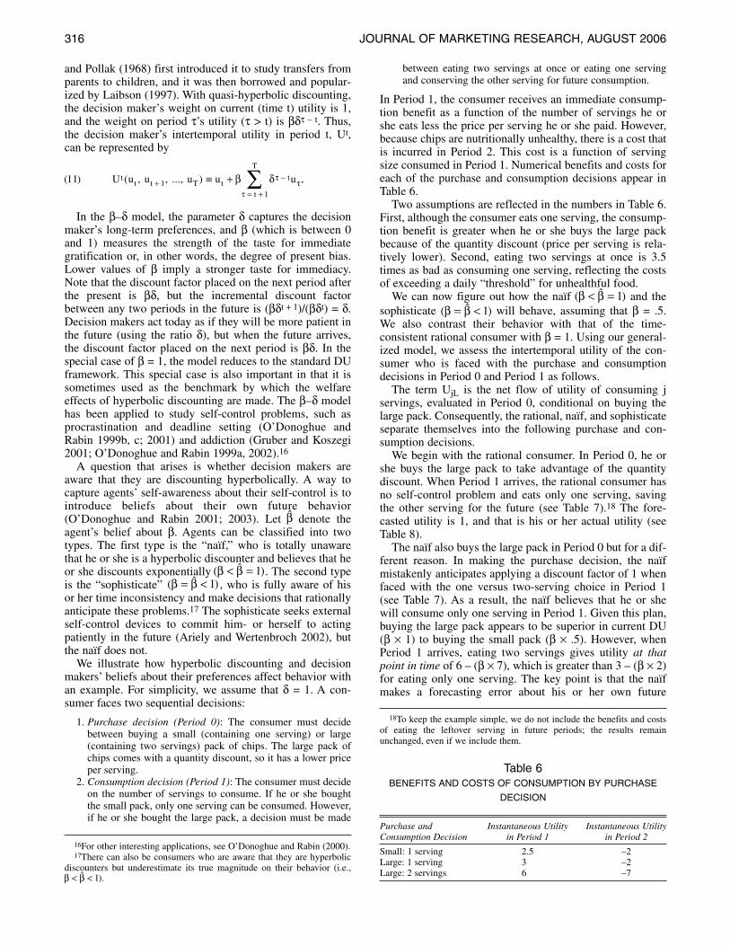
Small: 1 serving 2.5 –2Large: 1 serving 3.0 –2Large: 2 servings 6.0 –7
Table 6BENEFITS AND COSTS OF CONSUMPTION BY PURCHASE
DECISION
16For other interesting applications, see O’Donoghue and Rabin (2000).17There can also be consumers who are aware that they are hyperbolic
discounters but underestimate its true magnitude on their behavior (i.e.,β β< <ˆ ).1
and Pollak (1968) first introduced it to study transfers fromparents to children, and it was then borrowed and popular-ized by Laibson (1997). With quasi-hyperbolic discounting,the decision maker’s weight on current (time t) utility is 1,and the weight on period τ’s utility (τ > t) is βδτ – t. Thus,the decision maker’s intertemporal utility in period t, Ut,can be represented by
In the β–δ model, the parameter δ captures the decisionmaker’s long-term preferences, and β (which is between 0and 1) measures the strength of the taste for immediategratification or, in other words, the degree of present bias.Lower values of β imply a stronger taste for immediacy.Note that the discount factor placed on the next period afterthe present is βδ, but the incremental discount factorbetween any two periods in the future is (βδt + 1)/(βδt) = δ.Decision makers act today as if they will be more patient inthe future (using the ratio δ), but when the future arrives,the discount factor placed on the next period is βδ. In thespecial case of β = 1, the model reduces to the standard DUframework. This special case is also important in that it issometimes used as the benchmark by which the welfareeffects of hyperbolic discounting are made. The β–δ modelhas been applied to study self-control problems, such asprocrastination and deadline setting (O’Donoghue andRabin 1999b, c; 2001) and addiction (Gruber and Koszegi2001; O’Donoghue and Rabin 1999a, 2002).16
A question that arises is whether decision makers areaware that they are discounting hyperbolically. A way tocapture agents’ self-awareness about their self-control is tointroduce beliefs about their own future behavior(O’Donoghue and Rabin 2001; 2003). Let denote theagent’s belief about β. Agents can be classified into twotypes. The first type is the “naïf,” who is totally unawarethat he or she is a hyperbolic discounter and believes that heor she discounts exponentially . The second typeis the “sophisticate” , who is fully aware of hisor her time inconsistency and make decisions that rationallyanticipate these problems.17 The sophisticate seeks externalself-control devices to commit him- or herself to actingpatiently in the future (Ariely and Wertenbroch 2002), butthe naïf does not.
We illustrate how hyperbolic discounting and decisionmakers’ beliefs about their preferences affect behavior withan example. For simplicity, we assume that δ = 1. A con-sumer faces two sequential decisions:
1. Purchase decision (Period 0): The consumer must decidebetween buying a small (containing one serving) or large(containing two servings) pack of chips. The large pack ofchips comes with a quantity discount, so it has a lower priceper serving.
2. Consumption decision (Period 1): The consumer must decideon the number of servings to consume. If he or she boughtthe small pack, only one serving can be consumed. However,if he or she bought the large pack, a decision must be made
( ˆ )β β= < 1( ˆ )β β< = 1
β̂
( ) ( , , ..., )11 11
U u u u u utt t T t
t
t
T
+−
= +
≡ + ∑β δ ττ
τ
..
18To keep the example simple, we do not include the benefits and costsof eating the leftover serving in future periods; the results remainunchanged, even if we include them.
between eating two servings at once or eating one servingand conserving the other serving for future consumption.
In Period 1, the consumer receives an immediate consump-tion benefit as a function of the number of servings he orshe eats less the price per serving he or she paid. However,because chips are nutritionally unhealthy, there is a cost thatis incurred in Period 2. This cost is a function of servingsize consumed in Period 1. Numerical benefits and costs foreach of the purchase and consumption decisions appear inTable 6.
Two assumptions are reflected in the numbers in Table 6.First, although the consumer eats one serving, the consump-tion benefit is greater when he or she buys the large packbecause of the quantity discount (price per serving is rela-tively lower). Second, eating two servings at once is 3.5times as bad as consuming one serving, reflecting the costsof exceeding a daily “threshold” for unhealthful food.
We can now figure out how the naïf and thesophisticate will behave, assuming that β = .5.We also contrast their behavior with that of the time-consistent rational consumer with β = 1. Using our general-ized model, we assess the intertemporal utility of the con-sumer who is faced with the purchase and consumptiondecisions in Period 0 and Period 1 as follows.
The term UjL is the net flow of utility of consuming jservings, evaluated in Period 0, conditional on buying thelarge pack. Consequently, the rational, naïf, and sophisticateseparate themselves into the following purchase and con-sumption decisions.
We begin with the rational consumer. In Period 0, he orshe buys the large pack to take advantage of the quantitydiscount. When Period 1 arrives, the rational consumer hasno self-control problem and eats only one serving, savingthe other serving for the future (see Table 7).18 The fore-casted utility is 1, and that is his or her actual utility (seeTable 8).
The naïf also buys the large pack in Period 0 but for a dif-ferent reason. In making the purchase decision, the naïfmistakenly anticipates applying a discount factor of 1 whenfaced with the one versus two-serving choice in Period 1(see Table 7). As a result, the naïf believes that he or shewill consume only one serving in Period 1. Given this plan,buying the large pack appears to be superior in current DU(β × 1) to buying the small pack (β × .5). However, whenPeriod 1 arrives, eating two servings gives utility at thatpoint in time of 6 – (β × 7), which is greater than 3 – (β × 2)for eating only one serving. The key point is that the naïfmakes a forecasting error about his or her own future
( ˆ )β β= < 1( ˆ )β β< = 1

Modeling the Psychology of Consumer and Firm Behavior 317
Rational Naïf Sophisticate
Purchase Decision (Period 0)Small 2.5 – 2 β(2.5 – 2) β(2.5 – 2) Large Max{U1L, U2L) =
Max{3–2, 6–7}β × Max{U1L, U2L) =
β × Max{3–2, 6–7}β × Uj*L, where j* =
argmax{Large–j serving in Period 1}
Consumption Decision (Period 1)Small: 1 serving 2.5 – 2 2.5 – β × 2 2.5 – β × 2Large: 1 serving 0.3 – 2 0.3 – β × 2 0.3 – β × 2Large: 2 servings 0.6 – 7 0.6 – β × 7 0.6 – β × 7
Table 7UTILITIES OF THE CONSUMER GIVEN PURCHASE AND CONSUMPTION DECISIONS
Rational Naïf Sophisticate
Purchase Decision (Period 0) Large Large SmallSmall 0.5 .25 0.25Large 1.0 .50 –.50
Consumption Decision (Period 1) 1 Serving 2 Servings 1 Serving
Small: 1 serving n.a. n.a. 1.5Large: 1 serving 01 2.0 n.a.Large: 2 servings –1 2.5 n.a.
Notes: n.a. = not applicable.
Table 8DECISIONS AND UTILITIES OF THE CONSUMER (β = .5 FOR NAÏF AND SOPHISTICATE)
19However, it is not always the case that a sophisticated agent exhibitsmore self-control of this sort than a naïf does. O’Donoghue and Rabin(1999b) present examples in which sophisticated agents know they willsuccumb eventually and thus succumb sooner than the naive agents.
behavior: In period 0, the naïf chooses as if he or she will becomparing between utilities of 3 – 2 and 6 – 7 in Period 1,neglecting the β weight that will actually appear and dis-count the high future cost in Period 1, making the naïf eagerto eat both servings in one period. Note that as a result,actual utility, evaluated at Period 0, is not .5 but rather.5(6 – 7) = –.5.
The sophisticate forecasts accurately what will happen ifhe or she buys the large pack. That is, the Table 7 entries forutilities of consuming from the large pack when Period 1arrives are exactly the same for the naïf and the sophisti-cate. The difference is that the sophisticate anticipates thisactual choice when planning which pack to buy in Period 0.As a result, the sophisticate deliberately buys the smallpack, eats only one serving, and has both a forecasted andan actual DU of .25. The crucial point here is that the naïfdoes not plan to eat both servings, so he or she buys thelarge pack. The sophisticated knows that he or she cannotresist and thus buys the small pack.19
Marketing Application: Price Plans for Gym Memberships
Hyperbolic discounting is most likely to be found forproducts that involve either immediate costs with delayedbenefits (visits to the gym, health screenings) or immediatebenefits with delayed costs (smoking, using credit cards,eating) and temptation. Della Vigna and Malmendier (2004)examine the firm’s optimal pricing contracts in the presenceof consumers with hyperbolic preferences for gym member-ships. Their three-stage model is set up as follows.
At time t = 0, the monopolist firm offers the consumer aTPT with a membership fee F and a per-use fee p. The con-
20The unknown unit cost is just a modeling device to inject a probabilityof going to the gym or not into the analysis in a sensible way. It also cap-tures the case in which people are not genuinely sure about how much theywill dislike exercising or like the health benefits that result when they com-mit to a membership.
sumer either accepts or rejects the contract. If the consumerrejects the contract, he or she earns a payoff of u� at t = 1, thefirm earns nothing, and the game ends. If the consumeraccepts the contract, he or she pays F at t = 1 and thendecides between exercise (E) or nonexercise (N). If the con-sumer chooses E, he or she incurs a cost c and pays the firmthe usage fee p at t = 1. The consumer earns delayed healthbenefits b > 0 at t = 2. If he or she chooses N, the cost is 0,and the payoffs at t = 2 are also 0. It is assumed that theconsumer learns cost c at the end of t = 0, after he or she hasmade the decision to accept or reject the contract. However,before the consumer makes that decision, he or she knowsthe cumulative distribution G(c) from which c is drawn(G[c] is the probability that the consumer has a cost of c orless).20 The firm incurs a setup cost of K ≥ 0 whenever theconsumer accepts the contract and a unit cost a if the cus-tomer chooses E. The consumer is a hyperbolic discounterwith parameters . For simplicity, it is also assumedthat the firm is time consistent with a discount factor δ.
For the naive hyperbolic consumer choosing to exercise,the decision process can be described as follows: At t = 0,the utility from choosing E is βδ × (δb – p – c), and the pay-off from N is 0. Thus, the consumer chooses E if c ≤ δb – p.However, when t = 1 actually arrives, choosing E yieldsonly βδb – p – c, and thus the consumer actually chooses Eonly if c ≤ βδb – p. The naive hyperbolic consumer mispre-dicts his or her own future discounting process and thusoverestimates the net utility of E when buying the member-ship. The actual probability that the consumer chooses toexercise is the percentage chance that his or her cost is
( , ˆ , )β β δ

318 JOURNAL OF MARKETING RESEARCH, AUGUST 2006
below the cost threshold βδb – p, which is just G(βδb – p).Thus, the consumer chooses to exercise less often than he orshe plans to when buying the membership. The differencebetween the expected and the actual probability of exerciseis reflected by G(δb – p) – G(βδb – p). In addition, if anintermediate case in which the consumer can be partiallynaive about his or her time-inconsistent behavioris allowed, the degree by which the consumer overestimateshis or her probability of choosing E is –G(βδb – p). Unlike the naive or partially naive consumers, the fully sophisticated consumer (β = < 1) displays nooverconfidence about how often he or she will choose E.Overall, the consumer’s expected net benefit at t = 0 whenhe or she accepts the contract is βδ[–F + (δb – p –c)dG(c)].
The rational firm anticipates this, and its profit-maximization problem is given by
The “such that” constraint reflects the notion that as amonopolist, the firm can fix contract terms that make theconsumer indifferent between going and earning theexpected benefit or rejecting and earning the discountedrejection payoff βδu�. The firm maximizes its own dis-counted profits, which is the fixed fee F less its fixed costsK times the percentage of time it collects user fees becausethe consumer chooses E (the term G(βδb – p)) times the netprofit from the user fees p – a.
Della Vigna and Malmendier (2004) begin with the casein which consumers are time consistent (β = 1). Then, thefirm simply sets p* equal to marginal cost a and chooses F*to satisfy the consumer’s participation constraint (the afore-mentioned “such that” constraint). More interestingly, whenβ < 1, the firm’s optimal contract involves setting the per-use fee below marginal cost (p* < a) and the membershipfee F above the optimal level F* for time-inconsistent con-sumers. This result can be attributed to two reasons: First,the below-cost usage fee serves as a commitment device forthe sophisticate to increase his or her probability of exer-cise. The sophisticate likes paying a higher membership feecoupled with a lower per-use fee because the sophisticateknows that he or she will be tempted to skip the gym unlessthe per-use fee is low. Second, the firm can exploit thenaïf’s overconfidence about future exercise; the naïf willaccept the contract and pay F* but will exercise (and paysp* < a) less often than he or she believes. To support thesetheoretical results, Della Vigna and Malmendier presentedempirical evidence that shows that the industry for healthclub memberships typically charges high membership feesand low (and often zero) per-use fees. Furthermore, in theirstudy the average membership fee is approximately $300per year. For most gyms, consumers also have the option ofpaying no membership fee but a higher per-use fee(approximately $15 per visit). The average consumer whopaid a typical $300 fee goes to the gym so rarely that his orher effective per-use cost is $19 per visit; this consumerwould have been better off not buying the membership andjust paying on a per-use basis. This type of forecasting mis-take is precisely what the naive hyperbolic consumer does.
( ) max { ( )( )},
12F p
F K G b p p aδ βδ
βδsuch that
− + − −
− + ∫ − −⎡⎣⎢
⎤⎦⎥
=−∞−F b p c dG c ub pˆ
( ) ( ) .βδ δ βδ
∫ −∞−β̂δb p
β̂
G b p(ˆ )βδ −
( ˆ )β β< < 1
21For example, the predictions of NE in games with a unique mixed-strategy equilibrium are often close to the empirical results in aggregate.
NEW METHODS OF GAME-THEORETIC ANALYSES
Game theory is a mathematical system for analyzing andpredicting how people and firms will behave in strategic sit-uations. It has been a productive tool in many marketingapplications (Moorthy 1985). The field of game theory pri-marily uses the solution concept of NE and various refine-ments of it (i.e., mathematical additions that restrict the setof NE and provide more precision). Equilibrium analysismakes three assumptions: (1) “strategic thinking” (i.e.,players form beliefs based on an analysis of what othersmight do), (2) “optimization” (i.e., players choose the bestactions given those beliefs to maximize their payoffs), and(3) “mutual consistency” (i.e., players’ best responses andothers’ beliefs of their actions are identical [or, more sim-ply, players’ beliefs about what other players will do areaccurate]). Taken together, these assumptions impose a highdegree of rationality on the players in the game. Despitethese strong assumptions, NE is an appealing tool because itdoes not require the specification of any free parameter(when the game is defined) to arrive at a prediction. Fur-thermore, the theory is general because in games withfinitely many strategies and players, there is always someNE (sometimes more than one). Thus, for any marketingapplication, if the game is finite, the theory can be used toderive a precise prediction.
The advent of laboratory techniques to study economicbehavior that involves strategic interaction has enabledresearchers to test the predictive validity of NE in manyclasses of games, and hundreds of studies have been con-ducted (for a comprehensive review, see Camerer 2003).The accumulated evidence suggests that there are many set-tings in which NE does not explain actual behavior well,though in many other settings, it is remarkably accurate.21
The fact that NE sometimes fits poorly has spurredresearchers to look for alternative theories that are as pre-cise as NE but have more predictive power. These alterna-tive theories typically relax one or more of the strongassumptions underlying NE and introduce only one freeparameter that has a psychological interpretation.
In the following two sections, we introduce two alterna-tive solution concepts: quantal response equilibrium (QRE)(McKelvey and Palfrey 1995), which relaxes the assump-tion of optimization, and the cognitive hierarchy (CH)model (Camerer, Ho, and Chong 2004), which relaxes theassumption of mutual consistency. Both QRE and the CHmodel are one-parameter empirical alternatives to NE andhave been shown to predict more accurately than NE inhundreds of experimental games. We then describe the self-tuning experience-weighted attraction (EWA) learningmodel (Camerer and Ho 1998, 1999; Camerer, Ho, andChong 2002; Ho, Camerer, and Chong, in press). Thismodel relaxes both the best-response and the mutual consis-tency assumptions and describes precisely how playerslearn over time in response to feedback. The self-tuningEWA model nests the standard reinforcement and Bayesianlearning as special cases and is a general approach to modeladaptive learning behavior in settings in which people playan identical game repeatedly.

Modeling the Psychology of Consumer and Firm Behavior 319
B1 (q) B2 (1 – q)Empirical Frequency
(N = 128) NE QRE
A1 (p) 9, 0 0, 1 .54 .50 .65A2 (1 – p) 0, 1 1, 0 .46 .50 .35Empirical frequency .33 .67NE .10 .90QRE .35 .65
Table 9ASYMMETRIC HIDE-AND-SEEK GAME
22The data are taken from the first row of Table IX in McKelvey andPalfrey (1995).
23Assuming that the row player is mixing between A1 and A2 with prob-abilities p and 1 – p, the expected payoff for the column player fromchoosing B1 is p × 0 + (1 – p) × 1, and the expected payoff from choosingB2 is p × 1 + (1 – p) × 0. Equating the two expressions gives a solution p =.5. Similarly, the row player’s expected payoffs from A1 and A2 are q × 9 +(1 – q) × 0 and q × 0 + (1 – q) × 1. Equating the two expressions gives asolution q = .1.
QRE
Behavioral Regularities
Table 9 shows a game between two players. The rowplayer’s strategy space consists of Actions A1 and A2, andthe column player’s strategy space consists of Actions B1and B2. The game is a simple model of “hide-and-seek,” inwhich one player wants to match another player’s choice(e.g., A1 responding to B1), and another player wants tomismatch it (e.g., B1 responding to A2). The row playerearns either nine or one from matching on (A1, B1) or (A2,B2), respectively. The column player earns one from mis-matching on (A1, B2) or (A2, B1).
Table 9 also shows the empirical frequencies of each pos-sible action, averaged across many periods of an experimentconducted on this game.22 What is the NE prediction forthis game? We begin by observing that there is no pure-strategy NE for this game, so we look for a mixed-strategyNE. Suppose that the row player chooses A1 with probabil-ity p and A2 with probability 1 – p, and suppose that thecolumn player chooses B1 with probability q and B2 withprobability 1 – q. In a mixed-strategy equilibrium, the play-ers actually play a probabilistic mixture of the two strate-gies. If their valuation of outcomes is consistent withexpected utility theory, they prefer playing a mixture only ifthey are indifferent between each of their pure strategies.This property gives a way to compute the equilibrium mix-ture probabilities p and q. The mixed-strategy NE for thisgame turns out to be ([.5 A1, .5 A2], [.1 B1, .9 B2]).23 Com-paring this with the empirical frequencies, we find that NEprediction is close to actual behavior by the row players,whereas it underpredicts the choice of B1 for the columnplayers.
If one player plays a strategy that deviates from the pre-scribed equilibrium strategy, according to the optimizationassumption in NE, the other player must choose the bestresponse and deviate from NE as well. In this case,although the predicted NE and actual empirical frequenciesalmost coincide for the row player, the players are not play-ing an NE jointly, because the row player should haveplayed differently given that the column player deviated far
from the mixed-strategy NE (playing B1 33% of the timerather than 10%).
The Generalized Model
The QRE relaxes the assumption that players alwayschoose the best actions given their beliefs by incorporating“noisy” or “stochastic” best response. However, the theorybuilds in a sensible principle that actions with higherexpected payoffs are chosen more often; that is, players“better-respond” (cf. Fudenberg and Kreps 1993) ratherthan “best-respond.” Mathematically, the QRE nests NE asa special case, and it has a mathematically useful propertythat all actions are chosen with strictly positive probability(“anything can happen”). Behaviorally, this means that ifthere is a small chance that other players will do somethingirrational that has important consequences, players shouldtake this into account in a kind of robustness analysis.
The errors in the players’ QRE best-response functionsare usually interpreted as decision errors in the face of com-plex situations or as unobserved latent disturbances to theplayers’ payoffs (i.e., the players are optimizing given theirpayoffs, but there is a component of their payoff that onlythey understand). In other words, the relationship betweenQRE and NE is analogous to the relationship between sto-chastic choice and deterministic choice models.
To describe the concept more formally, suppose thatplayer i has Ji pure strategies indexed by j. Let πij be theprobability that player i chooses strategy j in equilibrium. AQRE is a probability assignment π (a set of probabilities foreach player and each strategy) such that for all i and j,πij = σij(u�i(π)), where u�i(.) is i’s expected payoff vector andσij(.) is a function mapping i’s expected payoff of strategy jonto the probability of strategy j (which depends on theform of the error distribution). A common functional formis the logistic quantal response function with σij(u�i) =
. In equilibrium, we have
where u�ij(π) is player i’s expected payoff from choosing jgiven that the other players choose their strategy accordingto the equilibrium profile π. It is easy to show mathemati-cally that πij is larger if the expected payoff u�ij(.) is larger(i.e., the better responses are played more often). Theparameter λ is the payoff sensitivity parameter. The extremevalue of λ = 0 implies that player i chooses among the Jistrategies equally often; that is, player i does not respond toexpected payoffs at all. At the other extreme, QREapproaches NE when λ → ∞, so that the strategy with the
( ) ,13
1
πλ
λij
u
uk
J
e
e
ij
iki
=×
×=∑
( )/( )e eu ukJij ikiλ λ× ×
=∑ 1

320 JOURNAL OF MARKETING RESEARCH, AUGUST 2006
highest expected payoff is played almost all the time. As λincreases, higher and higher probability is put on strategieswith better payoffs.
We now illustrate how to derive the QRE for a givenvalue of λ for the hide-and-seek game. Again, suppose thatthe row player chooses A1 with probability p and A2 withprobability 1 – p, and suppose that the column playerchooses B1 with probability q and B2 with probability 1 –q. Then, the expected payoffs from playing A1 and A2 areq × 9 + (1 – q) × 0 = 9q and q × 0 + (1 – q) × 1 = 1 – q,respectively. Therefore, we have πRowA1 = p = (eλ × 9q)/(eλ × 9q + eλ × (1 – q)). Similarly, the expected payoffs to B1and B2 for the column player are 1 – p and p, respectively,so we have πColumnB1 = q = (eλ × (1 – p))/(eλ × (1 – p) + eλ × p)).Note that q is on the right-hand side of the first equation,which determines p, and p is on the right-hand side of thesecond equation, which determines q. To a psychologist, thelogic might appear “circular” because p depends on q and qdepends on p, but that mutual dependence is what deliversmathematical precision. For any value of λ, there is onlyone pair of (p, q) values that solves the simultaneous equa-tions and yields a QRE. For example, if λ = 2, the QRE pre-dictions are p* = .646 and q* = .343, which are closer to theempirical frequencies than the NE predictions.
Using the actual data, a precise value of λ can be esti-mated using maximum-likelihood methods. The estimatedλ for the QRE model for the asymmetric hide-and-seekgame is 1.95. The negative of the log-likelihood of QRE (anoverall measure of goodness of fit) is 1721, a substantialimprovement over a random model benchmark (p = q = .5),which has a fit of 1774. The NE prediction has a fit of 1938,which is worse than random because of the extreme predic-tion of q = .1.
Marketing Application: Price Competition withDifferentiated Products
We now apply QRE to study price competition betweenfirms and contrast its predictions with NE. We adapt thisapplication from the work of Friedman, Palfrey, and Thisse(1995), who derive the QRE for a differentiated goodsBertrand duopoly. In this model, there are two firms thatchoose prices p1 and p2. After the firms choose pricessimultaneously, the quantity of products they sell is givenby two demand functions:
where a, b, and c > 0. For simplicity, we assume that themarginal cost of production for each firm is zero and thatc < 2b. That c > 0 implies that the two firms’ products areimperfect substitutes, so that if p2 is higher, consumers willdemand more of Product 1. We consider only the case inwhich the payoffs are nonnegative, so the firms’ strategyspace is the interval [0, (a/b)]. We can easily show that thesymmetric pure-strategy NE in which both firms choose thesame price is pNE = a/(2b – c). To begin deriving the QRE,let denote the firm’s expected price in the symmetric QREin which both firms choose the same distribution of prices.Friedman, Palfrey, and Thisse assume a quantal responsefunction as follows:
p
( ) ( , ) ,
( , )
14 1 1 2 1 2
2 1 2
q p p a bp cp
q p p a b
and= − +
= − pp cp2 1+ ,
where f(p) is the firm’s density function of prices over theinterval [0, (a/b)] and λ ≥ 0. To simplify the analysis, Fried-man, Palfrey, and Thisse solve for a QRE, assuming thatλ = 1. Letting , the expected price
in the symmetric QRE is
Furthermore,
Thus, is given implicitly by the following expression: =In solving this, we obtain =
(a/[6bc]) × [ – (b – 2c)]. In this case, wehave pNE > , because
is satisfied when c > 0. Thus, when λ = 1, QRE predictsprice dispersion and more competitive prices on averagethan the pure-strategy NE price. To understand this, notethat when players are pricing purely randomly (λ = 0), themean price is a/(2b), which is less than the pNE when c > 0.Because quantal response tends to drive prices downward,when one firm charges a lower price, the other firm wants toprice lower as well when products are substitutes. Fried-man, Palfrey, and Thisse also predict that is increasing inλ and approaches the NE solution when λ is large.
THE CH MODEL
Behavioral Regularities
In a dominance solvable game called the p-beauty contest(Ho, Camerer, and Weigelt 1998; Nagel 1995), a group ofplayers are each asked to pick a number from 0 to 100, andthe player who chooses a number that is closest to two-thirds the average of the numbers chosen by all players(including the player him- or herself) wins a cash prize. Ifthere is more than one winner (i.e., two or more playerschoose the same closest number), the prize is dividedequally. The NE prediction for this game is that all playerswill choose the number 0, and the reasoning for this is asfollows: “Even if everyone else picks 100, I should pick nomore than 67 (i.e., [2/3] × 100). However, all the other play-ers apply the same reasoning, so I should pick no more than45 (i.e., [2/3]2 × 100); but again, all the other players knowthis as well…,” and the choice of the player unravels to 0.The p-beauty contest has been played across diverse partici-pant groups. Table 10 gives a sample of the actual averagechoices from some of these groups.
The data show that the NE prediction of 0 explains first-period choices very poorly in this game. Furthermore,telling someone to play the equilibrium choice is badadvice. However, choices are heterogeneous across partici-
p
( ) ( ) ( )182 6
2 6 22a
b c
a
bcb c bc b c
−> − + − −⎡
⎣⎤⎦
p(b – 2c) + 6bc2
p( / ) ([ ]/[ ]).a b a cp a cp× + +4 2 6pp
( ) ( )172 30
2
K p a bp cp dpa
b
a cp aab= − + = ⎛
⎝⎜⎞⎠⎟
+ −⎛⎝⎜∫ ⎞⎞
⎠⎟.
( ) ( )( / )
.163 40
3p p f p dp
a b
K
a cp aab= × = + −⎛
⎝⎜⎞⎠⎟∫
pK p a bp cp dpa b= − +∫ ( )/
0
( ) ( )[ ( )]
[ ( )]
,15
0
f pp a bp cp
p a bp cp dpab
= − +
− +∫λ
λ
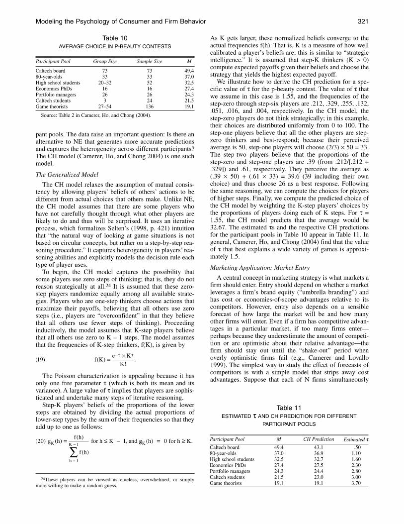
Modeling the Psychology of Consumer and Firm Behavior 321
Participant Pool Group Size Sample Size M
Caltech board 73 73 49.480-year-olds 33 33 37.0High school students 20–32 52 32.5Economics PhDs 16 16 27.4Portfolio managers 26 26 24.3Caltech students 3 24 21.5Game theorists 27–54 136 19.1
Source: Table 2 in Camerer, Ho, and Chong (2004).
Table 10AVERAGE CHOICE IN P-BEAUTY CONTESTS
Participant Pool M CH Prediction Estimated τCaltech board 49.4 43.1 .5080-year-olds 37.0 36.9 1.10High school students 32.5 32.7 1.60Economics PhDs 27.4 27.5 2.30Portfolio managers 24.3 24.4 2.80Caltech students 21.5 23.0 3.00Game theorists 19.1 19.1 3.70
Table 11ESTIMATED τ AND CH PREDICTION FOR DIFFERENT
PARTICIPANT POOLS
24These players can be viewed as clueless, overwhelmed, or simplymore willing to make a random guess.
pant pools. The data raise an important question: Is there analternative to NE that generates more accurate predictionsand captures the heterogeneity across different participants?The CH model (Camerer, Ho, and Chong 2004) is one suchmodel.
The Generalized Model
The CH model relaxes the assumption of mutual consis-tency by allowing players’ beliefs of others’ actions to bedifferent from actual choices that others make. Unlike NE,the CH model assumes that there are some players whohave not carefully thought through what other players arelikely to do and thus will be surprised. It uses an iterativeprocess, which formalizes Selten’s (1998, p. 421) intuitionthat “the natural way of looking at game situations is notbased on circular concepts, but rather on a step-by-step rea-soning procedure.” It captures heterogeneity in players’ rea-soning abilities and explicitly models the decision rule eachtype of player uses.
To begin, the CH model captures the possibility thatsome players use zero steps of thinking; that is, they do notreason strategically at all.24 It is assumed that these zero-step players randomize equally among all available strate-gies. Players who are one-step thinkers choose actions thatmaximize their payoffs, believing that all others use zerosteps (i.e., players are “overconfident” in that they believethat all others use fewer steps of thinking). Proceedinginductively, the model assumes that K-step players believethat all others use zero to K – 1 steps. The model assumesthat the frequencies of K-step thinkers, f(K), is given by
The Poisson characterization is appealing because it hasonly one free parameter τ (which is both its mean and itsvariance). A large value of τ implies that players are sophis-ticated and undertake many steps of iterative reasoning.
Step-K players’ beliefs of the proportions of the lowersteps are obtained by dividing the actual proportions oflower-step types by the sum of their frequencies so that theyadd up to one as follows:
( ) ( )( )
( )
–20 1
1
1g h
f h
f h
h KK
h
K= ≤
=
−
∑for , and gg h h KK ( ) for .= ≥0
( ) ( )!
.19 f Ke K
K= ×− τ τ
As K gets larger, these normalized beliefs converge to theactual frequencies f(h). That is, K is a measure of how wellcalibrated a player’s beliefs are; this is similar to “strategicintelligence.” It is assumed that step-K thinkers (K > 0)compute expected payoffs given their beliefs and choose thestrategy that yields the highest expected payoff.
We illustrate how to derive the CH prediction for a spe-cific value of τ for the p-beauty contest. The value of τ thatwe assume in this case is 1.55, and the frequencies of thestep-zero through step-six players are .212, .329, .255, .132,.051, .016, and .004, respectively. In the CH model, thestep-zero players do not think strategically; in this example,their choices are distributed uniformly from 0 to 100. Thestep-one players believe that all the other players are step-zero thinkers and best-respond; because their perceivedaverage is 50, step-one players will choose (2/3) × 50 = 33.The step-two players believe that the proportions of thestep-zero and step-one players are .39 (from .212/[.212 +.329]) and .61, respectively. They perceive the average as(.39 × 50) + (.61 × 33) = 39.6 (39 including their ownchoice) and thus choose 26 as a best response. Followingthe same reasoning, we can compute the choices for playersof higher steps. Finally, we compute the predicted choice ofthe CH model by weighting the K-step players’ choices bythe proportions of players doing each of K steps. For τ =1.55, the CH model predicts that the average would be32.67. The estimated τs and the respective CH predictionsfor the participant pools in Table 10 appear in Table 11. Ingeneral, Camerer, Ho, and Chong (2004) find that the valueof τ that best explains a wide variety of games is approxi-mately 1.5.
Marketing Application: Market Entry
A central concept in marketing strategy is what markets afirm should enter. Entry should depend on whether a marketleverages a firm’s brand equity (“umbrella branding”) andhas cost or economies-of-scope advantages relative to itscompetitors. However, entry also depends on a sensibleforecast of how large the market will be and how manyother firms will enter. Even if a firm has competitive advan-tages in a particular market, if too many firms enter—perhaps because they underestimate the amount of competi-tion or are optimistic about their relative advantage—thefirm should stay out until the “shake-out” period whenoverly optimistic firms fail (e.g., Camerer and Lovallo1999). The simplest way to study the effect of forecasts ofcompetitors is with a simple model that strips away costadvantages. Suppose that each of N firms simultaneously

322 JOURNAL OF MARKETING RESEARCH, AUGUST 2006
Figure 1COMPARISON OF CH PREDICTIONS WITH EMPIRICAL DATA
decides whether to enter a market or stay out (denoted as 1and 0, respectively). We denote the total market demand asd < N, where d is expressed as a fraction of the number offirms (i.e., 0 < d < 1). If d or fewer firms enter (i.e., supplyis equal to or less than demand), the entrants each earn aprofit of 1. If more than d firms enter (i.e., supply is greaterthan demand), all the entrants earn 0. If a firm does notenter, it earns a profit of .5.
To keep the mathematics simple, we assume that firmsare risk neutral and that there are infinitely many “atom-istic” entrants. In this case, firms care only about whetherthe fraction of others entering is above d or not: If the frac-tion of others entering is below d, the firm should enter, butif the fraction of others entering is above d, the firm is bet-ter off staying out and earning .5. The NE in this case is amixed-strategy equilibrium in which firms randomize andenter with probability d. When the number of firms is large(N → ∞), the law of large numbers implies that the fractionof entry is d.
In actual experiments conducted on market entry gamessuch as this one, there are three empirical regularities (seeCamerer 2003, Ch. 7; Rapoport and Seale, in press):
1. Entry tends to be monotonically increasing in demand d,even in one-shot games and early periods of repeated games;
2. There is too much entry for low values of d (relative to NE)and too little entry for high values of d; and
3. Individual profiles of entry rates for different d values inwithin-subject designs (in which players choose whether toenter for different d values) tend to show some simple stepfunctions and more jagged out-in-out-in step functions (e.g.,Rapoport, Seale, and Winter 2002).
The CH model can explain all these regularities. Tobegin, we denote the entry function of step-K firms for agiven demand d as e(K, d). This function maps the demandd and thinking step K into a decision either to enter (1) or tostay out (0). We denote the interim total entry function forall steps up to and including K as E(K, d). In the CH model,a step-K firm believes that it is competing against a normal-ized Poisson distribution of players that do 0, 1, 2, …, K – 1steps of thinking. Thus, the step-K firm believes that it isfacing an interim total entry rate of E(K – 1, d) = gK(h) × e(h, d). If E(K – 1, d) < d, the step-K firm shouldenter (e(K, d) = 1); if E(K – 1, d) > d, the firm should stayout (e(K, d) = 0). The CH model’s prediction of how manyfirms will enter for each value of d is the limiting case E(∞,d), which depends on the value of τ.
We now work through the first couple of steps of entrypredicted by the CH model. Step-zero firms will randomize,so their entry function is e(0, d) = .5 for all values of d(think of these firms as ignoring competitors or marketsize). Step-one firms believe that if d is below .5, there willbe too much entry (because e[0, d] = .5 > d), so they stayout. However, if d is above .5, they anticipate e(0, d) = .5 <d, so there will not be enough entry, and they can profit byentering. Step-two firms believe that they are facing a mix-ture of step-zero and step-one firms. In the Poisson CHmodel, the relative proportions of these two types of firmsare g2(0) = 1/(1 + τ) and g2(1) = τ/(1 + τ). For d < .5, theexpected interim entry function E(1, d) is g2(0) × .5 +g2(1) × 0 = .5/(1 + τ). Thus, when d < .5/(1 + τ), there is toomuch entry due to the entry by the step-zero firms, and sothe step-two firms stay out. However, when .5/(1 + τ) < d <
ΣhK
=−
01
.5, there is not enough entry because the step-zero firms’entry scared away the step-one firms, and thus the two-stepfirms enter. Similar calculations show that for d > .5, theexpected interim entry function is E(1, d) = g2(0) × .5 +g2(1) × 1 = (.5 + τ)/(1 + τ). Step-two firms stay out when.5 < d < (.5 + τ)/(1 + τ) and enter when d > (.5 + τ)/(1 + τ).If τ = 1.5, step-two firms enter for .2 < d < .5 and for d > .8.Figure 1 shows the full CH prediction for τ = 1.5 plottedagainst NE and the experimental data in Camerer, Ho, andChong (2004).
The CH model explains the first empirical regularity ofentry increasing in d as follows: Suppose that the game isplayed sequentially with a group of 20 firms. If the demandd is 40% (so that 8 of 20 firms can profit), after 8 firmsenter, the rest will stay out. Although the game is not actu-ally played sequentially, the higher-step firms anticipatewhat lower-step firms will do, which smoothes out the entryfunction in a “pseudosequential” way. It is as if the higher-step firms make entry decisions after the lower-step firmsdo, thus smoothing the entry function. In the CH model, thesecond regularity results because of the lingering effect ofthe zero-step firms, which overenter at low values of d andunderenter at high values of d. Regarding the third regular-ity, as firms do more steps of thinking, their entry functionsbecome more jagged, or nuanced; they are sensitive to sub-tle differences in which levels of demand d are attractive forentry. That the same CH model can explain both rapid equi-libration in the market entry games and the lack of equili-bration in the p-beauty contest shows the generality of themodel. Although the behavioral economics approach is gen-erally critical of the empirical limits of the rational choiceapproach, good models should also be able to explain whenrational choice emerges in the limit or surprisingly quickly,and the CH model can do so.

Modeling the Psychology of Consumer and Firm Behavior 323
LEARNING
Behavioral Regularities
Equilibrium concepts such as NE study behavior afterequilibration, at the point when players have come to guessaccurately what other players do. One force that producesequilibration is learning from feedback. That is, players’actions at a point in time reflect their prior experiences withthose actions, which are used to anticipate others’ futureactions. An example that illustrates learning is the “median-action” coordination game (see Van Huyck, Battalio, andBeil 1991). This game involves a group of n players, wheren is an odd number. The choice of each player i consists ofchoosing an integer action xi from 1 to 7. Let M denote themedian of all the players’ actions. The payoff function foreach player is given by πi(xi, M) = .1M – .05(M – xi)2 + .6.This game captures the key features of economic situationsin which there is a motive for conformity because playersare penalized for choosing an xi that is different from themedian M (through the penalty of .05[M – xi]2). At thesame time, players have a common incentive to coordinateon a higher median choice because of the premium .1Madded to profits. Thus, all the players want the median num-ber to be high, which creates a motive to choose a largenumber, but nobody wants to choose a number larger thanwhat they expect the median will be.
In this game, there are many NE. For each of the valuesfrom 1 to 7, if players believe that the median will equalthat value, the best response is xi = M, so the median M willresult. So all the integers from 1 to 7 are pure-strategy NE(there are many mixed equilibriums as well). In this exam-ple, the NE is not precise at all. This imprecision leavesroom for an empirical theory to pin down what happenswhen players play for the first time (as the CH theorydescribed previously) and to specify a path of play overtime as players learn. Before theories of limited strategizingand learning came along in behavioral game theory, how-ever, theorists were inclined to ask which general deductiveprinciples players might use to select among the many equi-libriums (these are called “selection principles”).
Three deductive principles of equilibrium selection maybe useful in predicting what players will choose in themedian-action game. The first selection principle is “payoffdominance”; that is, players will choose the equilibriumthat is best for everyone. The payoff-dominant equilibriumis for everyone to choose 7, earning $1.30 each. The secondselection principle is based on the concept that people willmaximize their “security” and choose the action whosesmallest payoffs are the largest (maximizing the minimumpayoff). Choosing 3 guarantees that a player will make aminimum of at least $.50, and because this is the highestguaranteed payoff for any strategy, the “maximin” ruleselects the strategy of 3. The third selection principle is theone-step rule we introduced previously in the CH model, inwhich people will choose the strategy with the highestexpected value, assuming all medians are equally likely.This rule selects the strategy of 4.
Van Huyck, Battalio, and Beil (1991) conducted sixexperimental sessions in which a group of nine playersmade decisions for ten periods for the game we justdescribed. The results exhibit four regularities: First, theprinciples of payoff dominance and secure (maximin)
actions are not supported; the medians were never 7 or 3 inany period; in fact, the medians for every period are either 4or 5. Second, the median choices in each session arestrongly influenced by the initial median (in all cases, thetenth-period median is exactly the initial first-periodmedian). Third, not only does pure-strategy NE fail to pro-vide a determinate prediction, but it also performs ratherpoorly because all the nine players chose the same action inonly 19 of the 60 total periods. Fourth, and most importantfor our purpose, equilibration seems to result from learningover time because the NE (in which all participants play thesame strategy in those 19 periods) is played in the later peri-ods. Next, we present a model that is able to capture someof these dynamics.
The Generalized Model
Before we begin, some notation is necessary. For playeri, there are mi strategies, denoted as sij (the jth strategy forplayer i). Strategies that i actually chooses in period t andthat all other players (denoted as –i) choose are si(t) ands–i(t), respectively. Player i’s ex post payoff of choosingstrategy sij in time t is πi(sij, s–i(t)), and the actual payoffreceived is πi(si(t), s–i(t)) ≡ πi(t). For player i, strategy j hasa numerical attraction Aij(t) at the end of period t afterupdating from the period’s experience, and Aij(0) is the ini-tial attraction before the game starts. Attractions of period tdetermine choice probabilities in period t + 1 through thefollowing logistic stochastic response function:
where λ measures the degree of payoff sensitivity. Note thatas in the QRE model we discussed previously, λ = 0 repre-sents random response, and λ = ∞ represents best response.In the self-tuning EWA model, attractions are updated by
where I[x, y] is an indicator function (equal to 1 if x = y and0 if otherwise; see Camerer and Ho 1998, 1999; Camerer,Ho, and Chong 2002; Ho, Camerer, and Chong, in press).That is, previous attractions are multiplied by an experienceweight N(t – 1), decayed by a weight φi(t), incrementedeither by the actual payoff received (when I[sij, si(t)] = 1) orby ξij(t) times the payoff that could have been received(when I[sij, si(t)] = 0), and normalized by dividing by φi(t) ×N(t – 1) + 1. Note that an equilibrium model is a specialcase of nonlearning in which the initial attractions Aij(0) arederived from equilibrium calculations, and the initialexperience weight N(0) is very large.
The EWA is a hybrid of reinforcement and fictitious play(belief-learning) models. Standard reinforcement modelsassume that only actual choices are reinforced (i.e., whenξij(t) = 0; Erev and Roth 1998). The weighted fictitious playbelief-learning model corresponds to a case in which allchoices are reinforced with equal weights (i.e., all forgonepayoffs are reinforced by a weight of ξij(t) =1). We initializeN(0) by setting it equal to one, and we update it according
( ) ( ) ( ) ( ) ( ) { ( )
[
22 1 1A t t N t A t tij i ij ij= × − × − + +(φ ξ
11 − × × )−ξ π φij ij i i ij i it I s s t s s t( )] [ , ( )]} [ , ( )] (( ) ( ) ,t N t× − +⎡⎣ ⎤⎦1 1
( ) ( ) ,( )
( )
21 1
1
P te
eij
A t
A tk
m
ij
iki
+ =×
×=∑λ
λ

324 JOURNAL OF MARKETING RESEARCH, AUGUST 2006
Figure 3PREDICTED FREQUENCIES OF THE SELF-TUNING EWA
MODEL
1 2
3 4
5 6
7 8
9 10 S1
S3
S5
S7
.0000
.1000
.2000
.3000
.4000
.5000
.6000
Strategy Period
Pro
bab
ility
Figure 2EMPIRICAL FREQUENCIES FOR THE MEDIAN ACTION GAME
1 2
3 4
5 6
7 8
9 10 S1
S3
S5
S7
.0000
.1000
.2000
.3000
.4000
.5000
.6000
Strategy Period
Pro
bab
ility
to N(t) = φi(t) × N(t – 1) + 1. The initial attractions Aij(0)are computed numerically using the CH model with τ = 1.5.
The change-detector function φi(t). The decay rate φi(t),which weights lagged attractions, is often called “forget-ting.” Although forgetting does occur, the more interestingvariation in φi(t) is a player’s perception of how quickly thelearning environment is changing. Therefore, the functionφi(t) should be capable of “detecting change.” When aplayer senses that other players are changing, a self-tuningφi(t) should dip down, putting less weight on old experi-ence. The core of the φi(t) change-detector function is a“surprise index,” which is the difference between otherplayers’ recent strategies and their strategies in previousperiods. We define a history vector across the other players’strategies k that records the historical frequencies (includ-ing the most recent period t) of the choices made by theother players. A vector element is hik(t) = (Σ t
τ = 1I[s–ik,s–i(τ)]/t. The recent “history” rik(t) is a vector of zeros andones, which has a one for strategy s–ik = s–i(t) and zeros forall other strategies s–ik (i.e., rik(t) = I[s–ik, s–i(t)]). The sur-prise index Si(t) = sums up thesquared deviations between the cumulative history vectorhik(t) and the immediate recent history vector rik(t) acrossall the strategies. This surprise index varies from zero totwo. To map it into a sensible change detection value, φi(t) =1 – .5 × Si(t) is used. Because Si(t) is between zero and two,φi(t) is always (weakly) between one and zero.
The attention function ξij(t). The parameter ξij(t) is theweight on forgone payoffs. Presumably, this is tied to the expost attention participants pay to alternative payoffs. Thosewho have limited attention are likely to focus on strategiesthat would have given higher payoffs than what they actu-ally received because these strategies represent missedopportunities. To capture this property, define ξij(t) = 1 ifπi(sij, s–i(t)) ≥ πi(t) and 0 if otherwise. That is, participantsreinforce chosen strategies (in which the payoff inequalityis always an equality) and all unchosen strategies that havebetter payoffs (in which the inequality is strict) with aweight of one. They reinforce unchosen strategies withequal or worse payoffs by zero. Note that this ξij(t) cantransform the self-tuning rule into special cases over time.If participants are strictly best responding (ex post), noother strategies have a higher ex post payoff, so ξij(t) = 0 forall strategies j that were not chosen, which reduces themodel to choice reinforcement. However, if participantsalways choose the worst strategy, then ξij(t) = 1, which cor-responds to weighted fictitious play. If participants chooseneither the best nor the worst strategy, the updating schemewill push them (probabilistically) toward strategies thatyield better payoffs, which is both characteristic of humanlearning and normatively sensible.
The self-tuning EWA model captures the dynamics of themedian-action game we described. Figure 2 shows theempirical frequency for each of the seven strategies acrosstime for all the six sessions. These aggregate data show thatthe initial choices were relatively more diffuse and convergetoward NE behavior (around 4 and 5) in the subsequentrounds. Figure 3 shows how the self-tuning EWA modeltracks these changes over time. Ho, Camerer, and Chong (inpress) also show how the same model captures learningdynamics in other games ranging from coordination,dominance-solvable games to games with a unique mixed-
( ( ) ( ))h t r tik ikkm i −−∑ 2
strategy equilibrium. So, as in economics and game theory,a single learning model has generality because it can beapplied to games with different structures.
Marketing Application: Price Matching with Loyalty
Capra and colleagues (1999) experimentally studied atype of price-matching competition (first introduced byBasu [1994]). In this game, two firms must choose an inte-ger price between marginal cost and a reservation price thatis common to all customers. If the prices are equal, each

Modeling the Psychology of Consumer and Firm Behavior 325
Figure 4EMPIRICAL FREQUENCIES FOR THE PRICE-MATCHING GAME
14
710
80
81~
90
91~
100
101~
110
111~
120
121~
130
131~
140
141~
150
151~
160
161~
170
171~
180
181~
190
191~
200
.1
0
.2
.3
.4
.5
.6
.7
.8
.9
Pro
bab
ility
Period
Strategy
Figure 5PREDICTED FREQUENCIES OF THE SELF-TUNING EWA
MODEL
14
710 0
.1
.2
.3
.4
.5
.6
.7
.8
.9
80
81~
90
91~
100
101~
110
111~
120
121~
130
131~
140
141~
150
151~
160
161~
170
171~
180
181~
190
191~
200
Pro
bab
ility
Period
Strategy
firm receives the common price as its payoffs (i.e., the salesvolume is normalized to one). If the prices are unequal,each firm receives the lower of the two prices. In addition,the firm that charges the lower price receives a bonus R, andthe firm that charges the higher price pays a penalty of R.Thus, this type of competition is akin to a duopoly, in whichthe two sellers promise customers that their posted pricesare the lowest and offer lowest-price guarantees in the formof price matching to underpin their claims. Because cus-tomers believe that firms that offer such guarantees have thelowest price (Jain and Srivastava 2000), the firm thatcharges the lowest price earns a goodwill reward, whereasthe high-price firm suffers a reputation loss when customerscompare their posted prices (for a generalization of thisgame, see Ho and Lim 2004). As long as R > 1, the uniqueNE for this game is that equilibrium prices will be at mar-ginal costs. The proof is simple: If another firm is expectedto choose a price P, by undercutting P by one unit, the lowerprice firm earns P – 1 + R, which is more than it can earn bymatching P (and therefore earning P) or overpricing (earn-ing P – R). Because both firms always want to undercut byone unit, in theory, there is a “race to the bottom.” Strik-ingly, this prediction is also invariant to the size of thepenalty/reward factor R.
Capra and colleagues (1999) tested the NE prediction ofthis game, varying R at six different levels (5, 10, 20, 25,50, and 80). Participants grouped randomly in pairs weretold to name a price from 80 to 200 simultaneously. Eachparticipant played the game for ten rounds for each level ofR. Figure 4 shows empirical frequencies for R = 50. A widerange of prices are posted in the early rounds. Prices gradu-ally fall to between 91 and 100 in rounds three through five,81 and 90 in rounds five through six, and toward the NEprediction of 80 in subsequent rounds. As Figure 5 shows,the self-tuning EWA model captures the data well. Giventhe initial dispersion of prices, it is able to capture the
dynamics of equilibration and the high proportion of NEoutcomes in the subsequent rounds (approximately 80%choose the NE in the final round).
MARKETING APPLICATIONS
In this article, we described a marketing-related applica-tion of each of the new models we presented. Our goal wasto show exactly how each new model is used and how itsapplication can lead to new insights. This section extendsour discussion and speculates on how these new tools canbe applied more broadly to determine and influence the fourmarketing-mix decisions (i.e., decisions on price, product,promotion, and place).
Price
The concepts of reference price and asymmetric priceeffects, which have been ascribed to reference dependenceand loss aversion, are well-known empirical regularities inmarketing (Hardie, Johnson, and Fader 1993; Kalyanaramand Winer 1995; Mayhew and Winer 1992; Winer 1986).Yet with the exception of the work of Greenleaf (1995),there has been virtually no analytical research on how pastprices or the magnitude of loss aversion affects firms’ pric-ing strategies, particularly in the contexts of competitionand intertemporal pricing. For example, does referencedependence predict that prices should move in cycles anddecline within each cycle, as in the case of a monopoly?More important, can marketing researchers formulate pric-ing strategies for reference-dependent customers for newproducts or products for which customers do not have pricehistories? Koszegi and Rabin (2004) developed a model ofreference-dependent preferences that assumes that the cus-tomer’s reference point is not based on past prices but onwhether he or she expects to purchase a certain product on a
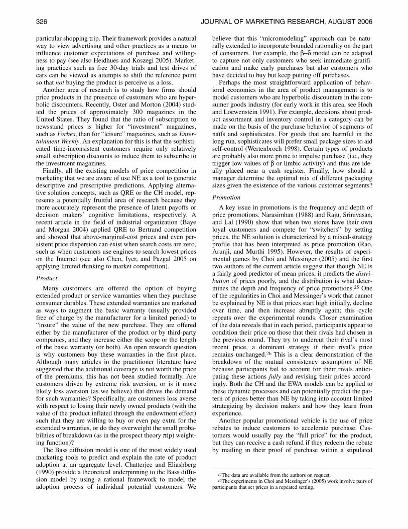
326 JOURNAL OF MARKETING RESEARCH, AUGUST 2006
particular shopping trip. Their framework provides a naturalway to view advertising and other practices as a means toinfluence customer expectations of purchase and willing-ness to pay (see also Heidhues and Koszegi 2005). Market-ing practices such as free 30-day trials and test drives ofcars can be viewed as attempts to shift the reference pointso that not buying the product is perceive as a loss.
Another area of research is to study how firms shouldprice products in the presence of customers who are hyper-bolic discounters. Recently, Oster and Morton (2004) stud-ied the prices of approximately 300 magazines in theUnited States. They found that the ratio of subscription tonewsstand prices is higher for “investment” magazines,such as Forbes, than for “leisure” magazines, such as Enter-tainment Weekly. An explanation for this is that the sophisti-cated time-inconsistent customers require only relativelysmall subscription discounts to induce them to subscribe tothe investment magazines.
Finally, all the existing models of price competition inmarketing that we are aware of use NE as a tool to generatedescriptive and prescriptive predictions. Applying alterna-tive solution concepts, such as QRE or the CH model, rep-resents a potentially fruitful area of research because theymore accurately represent the presence of latent payoffs ordecision makers’ cognitive limitations, respectively. Arecent article in the field of industrial organization (Bayeand Morgan 2004) applied QRE to Bertrand competitionand showed that above-marginal-cost prices and even per-sistent price dispersion can exist when search costs are zero,such as when customers use engines to search lowest priceson the Internet (see also Chen, Iyer, and Pazgal 2005 onapplying limited thinking to market competition).
Product
Many customers are offered the option of buyingextended product or service warranties when they purchaseconsumer durables. These extended warranties are marketedas ways to augment the basic warranty (usually providedfree of charge by the manufacturer for a limited period) to“insure” the value of the new purchase. They are offeredeither by the manufacturer of the product or by third-partycompanies, and they increase either the scope or the lengthof the basic warranty (or both). An open research questionis why customers buy these warranties in the first place.Although many articles in the practitioner literature havesuggested that the additional coverage is not worth the priceof the premiums, this has not been studied formally. Arecustomers driven by extreme risk aversion, or is it morelikely loss aversion (as we believe) that drives the demandfor such warranties? Specifically, are customers loss aversewith respect to losing their newly owned products (with thevalue of the product inflated through the endowment effect)such that they are willing to buy or even pay extra for theextended warranties, or do they overweight the small proba-bilities of breakdown (as in the prospect theory π(p) weight-ing function)?
The Bass diffusion model is one of the most widely usedmarketing tools to predict and explain the rate of productadoption at an aggregate level. Chatterjee and Eliashberg(1990) provide a theoretical underpinning to the Bass diffu-sion model by using a rational framework to model theadoption process of individual potential customers. We
25The data are available from the authors on request.26The experiments in Choi and Messinger’s (2005) work involve pairs of
participants that set prices in a repeated setting.
believe that this “micromodeling” approach can be natu-rally extended to incorporate bounded rationality on the partof consumers. For example, the β−δ model can be adaptedto capture not only customers who seek immediate gratifi-cation and make early purchases but also customers whohave decided to buy but keep putting off purchases.
Perhaps the most straightforward application of behav-ioral economics in the area of product management is tomodel customers who are hyperbolic discounters in the con-sumer goods industry (for early work in this area, see Hochand Loewenstein 1991). For example, decisions about prod-uct assortment and inventory control in a category can bemade on the basis of the purchase behavior of segments ofnaïfs and sophisticates. For goods that are harmful in thelong run, sophisticates will prefer small package sizes to aidself-control (Wertenbroch 1998). Certain types of productsare probably also more prone to impulse purchase (i.e., theytrigger low values of β or limbic activity) and thus are ide-ally placed near a cash register. Finally, how should amanager determine the optimal mix of different packagingsizes given the existence of the various customer segments?
Promotion
A key issue in promotions is the frequency and depth ofprice promotions. Narasimhan (1988) and Raju, Srinivasan,and Lal (1990) show that when two stores have their ownloyal customers and compete for “switchers” by settingprices, the NE solution is characterized by a mixed-strategyprofile that has been interpreted as price promotion (Rao,Arunji, and Murthi 1995). However, the results of experi-mental games by Choi and Messinger (2005) and the firsttwo authors of the current article suggest that though NE isa fairly good predictor of mean prices, it predicts the distri-bution of prices poorly, and the distribution is what deter-mines the depth and frequency of price promotions.25 Oneof the regularities in Choi and Messinger’s work that cannotbe explained by NE is that prices start high initially, declineover time, and then increase abruptly again; this cyclerepeats over the experimental rounds. Closer examinationof the data reveals that in each period, participants appear tocondition their price on those that their rivals had chosen inthe previous round. They try to undercut their rival’s mostrecent price, a dominant strategy if their rival’s priceremains unchanged.26 This is a clear demonstration of thebreakdown of the mutual consistency assumption of NEbecause participants fail to account for their rivals antici-pating these actions fully and revising their prices accord-ingly. Both the CH and the EWA models can be applied tothese dynamic processes and can potentially predict the pat-tern of prices better than NE by taking into account limitedstrategizing by decision makers and how they learn fromexperience.
Another popular promotional vehicle is the use of pricerebates to induce customers to accelerate purchase. Cus-tomers would usually pay the “full price” for the product,but they can receive a cash refund if they redeem the rebateby mailing in their proof of purchase within a stipulated

Modeling the Psychology of Consumer and Firm Behavior 327
period. An interesting issue is how rebate redemptionbehavior will change if firms vary the length of time theyallow customers to redeem the rebate and the monetary sizeof these rebates if the customers consist of naive andsophisticated hyperbolic discounters. For example, shouldthe profit-maximizing firm extend the redemption periodand increase the size of the rebate to attract the naïfs, know-ing that they are more likely to delay or forget (if it is afunction of delay) to redeem the rebate and end up payingthe full price? Furthermore, how should this be reconciledwith the desires of the sophisticates for tighter redemptiondeadlines or even “instant” rebates as forms of commitmentdevices? These questions have yet to be formally analyzed.
Place
The study of marketing distribution channels has beenheavily dominated by theoretical modeling. Compared withareas such as consumer behavior, there is relatively littleempirical research on channels. The study of channels pres-ents marketing researchers with unique opportunities tocombine empirical and especially experimental work(Anderson and Coughlan 2002) with the modeling tools inbehavioral economics. Existing models of channel relation-ships can be generalized following careful empirical studiesthat challenge the predictions of orthodox economic theory.
For example, firms in an independent channel cannotcapture all the possible profits in the channel by using a lin-ear price contract (this is the DM problem we mentionedpreviously). Pioneering work by Jeuland and Shugan (1983)and Moorthy (1987) shows theoretically that more complexnonlinear contracts, such as quantity discounts and TPTs,can eliminate the DM problem. A fundamental question thatarises from this stream of research is, Given that there aremany forms of quantity discount contracts that are used inpractice, should some contracts be preferred over others?Using experimental economics methodology, Lim and Ho(2006) compare two popular quantity discount contracts,the two-block and the three-block declining tariffs, whichare theoretically equally effective at solving the DM prob-lem. They find that the three-block tariff yields higher chan-nel profits than the two-block tariff. They show that theresults are consistent with a QRE in which the downstreamfirm in the channel also cares about the additional profits itwould have earned if the lower marginal price in a givenblock were to be applied to other blocks with higher mar-ginal prices.
In a different behavioral approach to DM, Cui, Raju, andZhang (2004) note that the DM problem may not createinefficiency in practice, even with a linear price contract, ifchannel members are not purely self-interested. They showthat if firms are sufficiently inequity averse (as in Fehr andSchmidt 1999), the efficient outcome that is reached by avertically integrated monopoly can be achieved with sepa-rate firms, so that complex nonlinear contracts aresuperfluous.
RESEARCH IMPLICATIONS
In this article, we show how the standard utility functionof decision makers such as customers or managers can begeneralized to capture three well-established empiricalregularities about people: They care about both absolute
outcomes and changes in outcomes relative to some refer-ence point, they care about both their own and others’ pay-offs, and they exhibit a taste for immediate gratification.These utility modifications have been increasingly popularin economics because they have one or two additionalparameters over the standard models, which make themamenable to empirical testing and estimation. We also pro-vide three alternatives to the standard NE solution conceptsin competitive situations. The QRE generalizes the standardequilibrium concepts by allowing decision makers to better-respond instead of best-respond. The CH model relaxes themutual consistency assumption of NE to allow decisionmakers to encounter surprises (because their beliefs of whatothers will do may not be the same as what others actuallydo). The self-tuning EWA model captures how decisionmakers might respond to experience over time when theycompete in repeated interactions. All these models comewith only one (in most cases) or two additional parametersthat can be empirically estimated.
We emphasize that the proposed models are by no meansthe final or complete models that capture all documentedbehavioral regularities. Research in psychology and eco-nomics is still actively delineating the boundaries of thesebehavioral regularities (see, e.g., Novemsky and Kahneman[2005] on loss aversion). It is also important to continue totest the predictions of standard models. More tests lead tomore facts about when and how the standard models fail(and when they succeed), which are useful because behav-ioral alternatives are still being proposed and refined. Teststhat include rational models as special cases also give esti-mates of the values of the additional parameters introducedin the behavioral models and can serve as a check ofwhether these behavioral models are well specified (e.g.,showing whether the parameter values obtained from thedata are psychologically plausible). The recent trend towardtesting well-specified theories in the laboratory (e.g., Amal-doss et al. 2000; Ghosh and John 2000; Ho and Zhang2004; Lim and Ho 2006; Srivastava, Chakravarti, andRapoport 2000) is a promising avenue for further researchand often makes it easier to separate rational and behavioralpredictions clearly.
Implications for Behavioral Researchers
We believe that it is crucial for behavioral researchers tocontinue to document robust violations of standard models.However, showing the existence of an important behavioralregularity is only the necessary first step toward its wideapplicability in marketing. To receive wide applicability, itis necessary that the regularity be precisely specified in aformal model. This formal specification process requires anactive collaboration between behavioral and quantitativeresearchers. Such collaboration, whether in the form ofcoauthorship or mutual influence from a common under-standing of facts and modeling language, is a promisingarea for further research. This article also implies that it isimportant for behavioral researchers to demonstrate impor-tant behavioral regularities in the field. The field experi-mentation approach allows researchers to test the idea thatbounded rationality may not survive in the marketplacebecause it rewards rationality more.

328 JOURNAL OF MARKETING RESEARCH, AUGUST 2006
Implications for Empirical Researchers
Empirical researchers in marketing have been successfulin testing standard economic models using field data sets.We believe that our proposed revised utility functionsshould be used in future empirical testing because they nestthe standard models. The empirical tests will provide usefulinformation as to when and how the standard models fail.We believe that this is an extremely fertile area of research.The QRE and the CH model can be used to study off-equilibrium path behavior in the framework of new empiri-cal industrial organization, which is an active area ofresearch in marketing. These revised models allowresearchers to check a foundational assumption of the fieldempirically; that is, firms always play pure equilibriumstrategies and never encounter surprises and make mistakes.We speculate that this standard assumption is likely to betrue in mature industries but less so in developing indus-tries. There is also room for applying the EWA learningmodels to capture how managers and customers learn overtime. For example, Ho and Chong (2003) apply the EWAmodel to predict consumers’ product choices and show thatit outperforms several existing models, including that ofGuadagni and Little (1983), using an extensive data setinvolving more than 130,000 purchases across 16 productcategories.
Implications for Analytical Researchers
We believe that there is an opportunity for analyticalmodelers to incorporate the revised utility functions in theirmodeling work. For example, it would be fruitful to investi-gate how a firm’s marketing-mix actions change when itfaces a group of customers who have reference-dependentpreferences, care about fairness, and are impatient. Howwould the market structure and degree of competition varyas a result of these changes? We believe that incorporatingthese changes might provide explanations for what seemlike market paradoxes that cannot be explained using stan-dard economic models. For example, Rotemberg (2005)shows that if customers care about fairness, it is optimal forfirms to engage in temporary sales events, and they shouldannounce their intention of increasing prices before actuallydoing so. Similarly, we believe that analytical modelers canapply both QRE and the CH model to analyze how firmsmight compete in a specific market setting. These modelswill allow researchers to capture behavior that would other-wise be suppressed by the stringent requirements of no sur-prises and zero mistakes. Both methods seem particularlypromising in modeling rapidly changing product marketsand in markets in which firms may not have a sufficientknowledge of actual demand and supply conditions.
In addition to the six topics we have narrowly focusedon, there are many more rich questions about the applicabil-ity of behavioral economics to market-level outcomes thatmarketing modelers are well-equipped to study. A rapidlyemerging question is how firms should make marketing-mix choices when consumers exhibit various types ofbounds on rationality. As Ellison (2005) notes, if consumersexhibit various biases relative to rational choice, from thefirm’s point of view, such biases will have the same practi-cal importance as product differentiation, though an identi-cal product might be differentiated by idiosyncrasies in con-sumer cognition rather than in tastes. This insight suggests
that familiar models could be adapted to study the behav-ioral economics of firm marketing behavior in the face ofconsumer rationality limits.
REFERENCES
Ainslie, George (1975), “Specious Reward: A Behavioral Theoryof Impulsiveness and Impulse Control,” Psychological Bulletin,82 (4), 463–96.
Akerlof, George and Janet Yellen (1990), “The Fair Wage-EffortHypothesis and Unemployment,” Quarterly Journal of Econom-ics, 105 (2), 255–83.
Amaldoss, Wilfred, Robert Meyer, Jagmohan Raju, and AmnonRapoport (2000), “Collaborating to Compete a Game-TheoreticModel and Experimental Investigation of the Effect of Profit-Sharing Arrangement and Type of Alliance,” Marketing Science,19 (2), 105–126.
Anderson, Erin and Anne Coughlan (2002), “Channel Manage-ment: Structure, Governance and Relationship Management,” inHandbook of Marketing, Barton Weitz and Robin Wensley, eds.London: Sage Publications, 223–47.
Ariely, Dan and Klaus Wertenbroch (2002), “Procrastination,Deadlines, and Performance: Self-Control by Precommitment,”Psychological Science, 13 (3), 219–24.
Barberis, Nicholas and Richard Thaler (2003), “A Survey ofBehavioral Finance,” in Handbook of the Economics of Finance,George Constantinides, Milton Harris, and Rene Stultz, eds.Amsterdam: Elsevier Science, North Holland, 1053–1128.
Basu, Amiya, Rajiv Lal, V. Srinivasan, and Richard Staelin (1985),“Salesforce Compensation Plans: An Agency Theoretic Per-spective,” Marketing Science, 4 (4), 267–91.
Basu, Kaushik (1994), “The Traveler’s Dilemma: Paradoxes ofRationality in Game Theory,” American Economic Review, 84(2), 391–95.
Bateman, Ian, Daniel Kahneman, Alistair Munro, Chris Starmer,and Robert Sugden (2005), “Testing Competing Models of LossAversion: An Adversarial Collaboration,” Journal of PublicEconomics, 89 (8), 1561–80.
Baye, Michael and John Morgan (2004), “Price-Dispersion in theLab and on the Internet: Theory and Evidence,” RAND Journalof Economics, 35 (3), 449–66.
Benartzi, Shlomo and Richard Thaler (1995), “Myopic Loss Aver-sion and the Equity Premium Puzzle,” Quarterly Journal ofEconomics, 110 (1), 73–92.
Benzion, Uri, Amnon Rapoport, and Joseph Yagil (1989), “Dis-count Rates Inferred from Decisions: An Experimental Study,”Management Science, 35 (3), 270–84.
Bolton, Gary and Axel Ockenfels (2000), “ERC: A Theory ofEquity, Reciprocity and Competition,” American EconomicReview, 90 (1), 166–93.
Bradlow, Eric T., Ye Hu, and Teck-Hua Ho (2004a), “A Learning-Based Model for Imputing Missing Levels in Partial ConjointProfiles,” Journal of Marketing Research, 41 (November),369–81.
———, ———, and ——— (2004b), “Modeling BehavioralRegularities of Consumer Learning in Conjoint Analysis,” Jour-nal of Marketing Research, 41 (November), 392–96.
Camerer, Colin (1999), “Behavioral Economics: Reunifying Psy-chology and Economics,” Proceedings of the National Academyof Sciences, 96 (19), 10575–77.
——— (2001), “Prospect Theory in the Wild: Evidence from theField,” in Choices, Values and Frames, Daniel Kahneman andAmos Tversky, eds. Cambridge, UK: Cambridge UniversityPress, 288–300.
——— (2003), Behavioral Game Theory: Experiments in Strate-gic Interaction. Princeton, NJ: Princeton University Press.
——— (2005), “Three Cheers—Psychological, Theoretical,Empirical—for Loss Aversion,” Journal of Marketing Research,42 (May), 129–33.

Modeling the Psychology of Consumer and Firm Behavior 329
———, Linda Babcock, George Loewenstein, and Richard Thaler(1997), “Labor Supply of New York City Cab Drivers: One Dayat a Time,” Quarterly Journal of Economics, 112 (2), 407–442.
——— and Teck Ho (1998), “EWA Learning in CoordinationGames: Probability Rules, Heterogeneity, and Time Variation,”Journal of Mathematical Psychology, 42 (2), 305–326.
——— and ——— (1999), “Experience-Weighted AttractionLearning in Normal Form Games,” Econometrica, 67 (4),837–74.
———, ———, and Juin-Kuan Chong (2002), “SophisticatedEWA Learning and Strategic Teaching in Repeated Games,”Journal of Economic Theory, 104 (1), 137–88.
———, ———, and ——— (2004), “A Cognitive HierarchyModel of Games,” Quarterly Journal of Economics, 119 (3),861–98.
———, Samuel Issacharoff, George Loewenstein, and TedO’Donoghue (2003), “Regulation for Conservatives: BehavioralEconomics and the Case for Asymmetric Paternalism,” Univer-sity of Pennsylvania Law Review, 151 (3), 1211–54.
———, George Loewenstein, and Matthew Rabin (2003),Advances in Behavioral Economics. Princeton, NJ: RussellSage Foundation/Princeton University Press.
——— and Dan Lovallo (1999), “Overconfidence and ExcessEntry: An Experimental Approach,” American EconomicReview, 89 (1), 306–318.
——— and Ulrike Malmendier (in press), “Behavioral Economicsof Organizations,” in Economic Institutions and BehavioralEconomics, Peter Diamond and Hannu Vartiainen, eds. Prince-ton, NJ: Princeton University Press.
Capra, Monica, Jacob Goeree, Rosario Gomez, and Charles Holt(1999), “Anomalous Behavior in a Traveler’s Dilemma?” Amer-ican Economic Review, 89 (3), 678–90.
Charness, Gary and Matthew Rabin (2002), “UnderstandingSocial Preferences with Simple Tests,” Quarterly Journal ofEconomics, 117 (3), 817–69.
Chatterjee, Rabikar and Jehoshua Eliashberg (1990), “The Innova-tion Diffusion Process in a Heterogeneous Population: A Micro-modeling Approach,” Management Science, 36 (9), 1057–1079.
Chen, Keith, Venkat Lakshminarayanan, and Laurie Santos(2005), “The Evolution of Our Preferences: Evidence fromCapuchin-Monkey Trading Behavior,” working paper, YaleSchool of Management.
Chen, Yuxin, Ganesh Iyer, and Amit Pazgal (2005), “LimitedMemory and Market Competition,” working paper, Haas Schoolof Business, University of California, Berkeley.
Choi, Sungchul and Paul Messinger (2005), “Edgeworth Promo-tional Cycles in the Loyal-Switcher Game,” working paper,Marketing Department, University of Alberta.
Chua, Zikang and Colin Camerer (2004), “Experiments onIntertemporal Consumption with Habit Formation and SocialLearning,” working paper, Division of Humanities and SocialSciences, California Institute of Technology.
Cui, Haitao, Jagmohan Raju, and John Zhang (2004), “Fairnessand Channel Coordination,” working paper, Marketing Depart-ment, Wharton School, University of Pennsylvania.
Degeorge, Francois, Jayendu Patel, and Richard Zeckhauser(1999), “Earnings Management to Exceed Thresholds,” Journalof Business, 72 (1), 1–33.
Della Vigna, Stefano and Ulrike Malmendier (2004), “ContractDesign and Self-Control: Theory and Evidence,” QuarterlyJournal of Economics, 119 (2), 353–402.
Dufwenberg, Martin and Georg Kirchsteiger (2004), “A Theory ofSequential Reciprocity,” Games and Economics Behavior, 47(2), 268–98.
Ellison, Glenn (2005), “Bounded Rationality in Industrial Organi-zation,” paper presented at the 2005 Econometric Society WorldCongress, University College London (August 19–24),(accessed April 12, 2006), [available at www.econ.ucl.ac.uk/eswc2005].
Erev, Ido and Alvin Roth (1998), “Predicting How People PlayGames: Reinforcement Learning in Experimental Games withUnique Mixed-Strategy Equilibria,” American EconomicReview, 88 (4), 848–81.
Fehr, Ernst, Alexander Klein, and Klaus Schmidt (2004), “Con-tracts, Fairness and Incentives,” Discussion Paper No. 2004-07,Department of Economics, University of Munich.
——— and Klaus Schmidt (1999), “A Theory of Fairness, Com-petition and Cooperation,” Quarterly Journal of Economics,114 (3), 817–68.
Frederick, Shane, George Loewenstein, and Ted O’Donoghue(2002), “Time Discounting and Time Preference: A CriticalReview,” Journal of Economic Literature, 40 (2), 351–401.
Friedman, James, Thomas Palfrey, and Jacques-Francois Thisse(1995), “Random Choice Behavior in Continuum Models,”research note, Department of Economics, University of NorthCarolina.
Friedman, Milton (1953), “The Methodology of Positive Econom-ics,” in Essays in Positive Economics, Milton Friedman, ed.Chicago: University of Chicago Press, 3–43.
Fudenberg, Drew and David Kreps (1993), “Learning Mixed Equi-libria,” Games and Economic Behavior, 5 (3), 320–67.
Genesove, David and Christopher Mayer (2001), “Loss Aversionand Seller Behavior: Evidence from the Housing Market,”Quarterly Journal of Economics, 116 (4), 1233–60.
Ghosh, Mrinal and George John (2000), “Experimental Evidencefor Agency Models of Salesforce Compensation,” MarketingScience, 19 (4), 348–65.
Greenleaf, Eric (1995), “The Impact of Reference Price Effects onthe Profitability of Price Promotions,” Marketing Science, 14(1), 82–104.
Gruber, Jonathan and Botond Koszegi (2001), “Is Addiction Ratio-nal? Theory and Evidence,” Quarterly Journal of Economics,116 (4), 1261–1305.
Guadagni, Peter and John Little (1983), “A Logit Model of BrandChoice Calibrated on Scanner Data,” Marketing Science, 2 (3),203–238.
Hardie, Bruce, Eric Johnson, and Peter Fader (1993), “ModelingLoss Aversion and Reference Dependence Effects on BrandChoice,” Marketing Science, 12 (4), 378–94.
Heidhues, Paul and Botond Koszegi (2005), “The Impact of Con-sumer Loss Aversion on Pricing,” working paper, Department ofEconomics, University of California, Berkeley.
Ho, Teck, Colin Camerer, and Juin-Kuan Chong (in press), “Self-Tuning Experience Weighted Attraction Learning in Games,”Journal of Economic Theory.
———, ———, and Keith Weigelt (1998), “Iterated Dominanceand Iterated Best-Response in p-Beauty Contests,” AmericanEconomic Review, 88 (4), 947–69.
——— and Juin-Kuan Chong (2003), “A Parsimonious Model ofSKU Choice,” Journal of Marketing Research, 40 (August),351–65.
——— and Noah Lim (2004), “A Theory of Lowest-Price Guar-antees,” working paper, Marketing Department, Haas School ofBusiness, University of California, Berkeley.
——— and Juan-Juan Zhang (2004), “Does the Format of PricingContracts Matter?” working paper, Marketing Department,Haas School of Business, University of California, Berkeley.
Hoch, Stephen and George Loewenstein (1991), “Time-Inconsistent Preferences and Consumer Self-Control,” Journalof Consumer Research, 17 (4), 492–507.
Holcomb, James and Paul Nelson (1992), “Another ExperimentalLook at Individual Time Preference,” Rationality and Society, 4(2), 199–220.
Jain, Sanjay and Joydeep Srivastava (2000), “An Experimental andTheoretical Investigation of Price-Matching Refund Policies,”Journal of Marketing Research, 37 (August), 351–62.
Jeuland, Abel and Steven Shugan (1983), “Managing ChannelProfits,” Marketing Science, 2 (3), 239–72.

330 JOURNAL OF MARKETING RESEARCH, AUGUST 2006
Kahneman, Daniel, Jack Knetsch, and Richard Thaler (1990),“Experimental Tests of the Endowment Effect and the CoaseTheorem,” Journal of Political Economy, 98 (6), 1325–48.
——— and Amos Tversky (1979), “Prospect Theory: An Analysisof Decision Under Risk,” Econometrica, 47 (2), 263–91.
——— and ——— (1992), “Advances in Prospect Theory:Cumulative Representation of Uncertainty,” Journal of Risk andUncertainty, 5 (4), 297–324.
Kalyanaram, Gurumurthy and Russell Winer (1995), “EmpiricalGeneralizations from Reference Price and Asymmetric PriceResponse Research,” Marketing Science, 14 (3), G161–69.
Kivetz, Ran, Oded Netzer, and V. Srinivasan (2004), “AlternativeModels for Capturing the Compromise Effect,” Journal of Mar-keting Research, 41 (August), 237–57.
Koszegi, Botond and Matthew Rabin (2004), “A Model ofReference-Dependent Preferences,” working paper, Departmentof Economics, University of California, Berkeley.
Laibson, David (1997), “Golden Eggs and Hyperbolic Discount-ing,” Quarterly Journal of Economics, 112 (2), 443–77.
Leeflang, Peter, Dick Wittink, Michel Wedel, and Philippe Naert,eds. (2000), Building Models for Marketing Decisions. NewYork: Kluwer Academic Publishers.
Lim, Noah and Teck Ho (2006), “Designing Price Contracts forBoundedly Rational Customers: Does the Number of BlocksMatter?” working paper, Marketing Department, Haas Schoolof Business, University of California, Berkeley.
Little, John (1970), “Models and Managers: The Concept of aDecision Calculus,” Management Science, 16 (8), B466–85.
Loewenstein, George (1987), “Anticipation and the Valuation ofDelayed Consumption,” Economic Journal, 97 (387), 666–84.
——— and Drazen Prelec (1992), “Anomalies in IntertemporalChoice: Evidence and an Interpretation,” Quarterly Journal ofEconomics, 107 (2), 573–97.
——— and ——— (1993), “Preferences for Sequences of Out-comes,” Psychological Review, 100 (1), 91–108.
——— and Richard Thaler (1989), “Anomalies: IntertemporalChoice,” Journal of Economic Perspectives, 3 (4), 181–93.
Mayhew, Glenn and Russell Winer (1992), “An Empirical Analy-sis of Internal and External Reference Price Effects Using Scan-ner Data,” Journal of Consumer Research, 19 (1), 62–70.
McClure, Samuel, David Laibson, George Loewenstein, andJonathan Cohen (2004), “Separate Neural Systems Value Imme-diate and Delayed Monetary Rewards,” Science, 306 (5695),503–507.
McFadden, Daniel (1999), “Rationality for Economists,” Journalof Risk and Uncertainty, 19 (1–3), 73–105.
McKelvey, Richard and Thomas Palfrey (1995), “QuantalResponse Equilibria for Normal Form Games,” Games andEconomic Behavior, 10 (1), 6–38.
Moorthy, Sridhar (1985), “Using Game Theory to Model Compe-tition,” Journal of Marketing Research, 22 (August), 262–82.
——— (1987), “Managing Channel Profits: Comment,” Market-ing Science, 6 (4), 375–79.
Nagel, Rosemarie (1995), “Unraveling in Guessing Games: AnExperimental Study,” American Economic Review, 85 (5),1313–26.
Narasimhan, Chakravarti (1988), “Competitive PromotionalStrategies,” Journal of Business, 61 (4), 427–49.
Novemsky, Nathan and Daniel Kahneman (2005), “The Bound-aries of Loss Aversion,” Journal of Marketing Research, 42(May), 119–28.
Odean, Terence (1998), “Are Investors Reluctant to Realize TheirLosses?” Journal of Finance, 53 (5), 1775–98.
O’Donoghue, Ted and Matthew Rabin (1999a), “Addiction andSelf-Control,” in Addiction: Entries and Exits, Jon Elster, ed.New York: Russell Sage Foundation, 169–206.
——— and ——— (1999b), “Doing It Now or Later,” AmericanEconomic Review, 89 (1), 103–124.
——— and ——— (1999c), “Incentives for Procrastinators,”Quarterly Journal of Economics, 114 (3), 769–816.
——— and ——— (2000), “The Economics of Immediate Grati-fication,” Journal of Behavioral Decision Making, 13 (2),233–50.
——— and ——— (2001), “Choice and Procrastination,” Quar-terly Journal of Economics, 116 (1), 121–60.
——— and ——— (2002), “Addiction and Present-Biased Prefer-ences,” working paper, Department of Economics, CornellUniversity.
——— and ——— (2003), “Self Awareness and Self Control,” inTime and Decision: Economic and Psychological Perspectiveson Intertemporal Choice, Roy Baumeister, George Loewen-stein, and Daniel Read, eds. New York: Russell Sage Founda-tion, 217–43.
Oster, Sharon and Fiona Scott Morton (2004), “Behavioral Deci-sion Making: An Application to the Setting of Magazine Sub-scription Prices,” working paper, Yale School of Management.
Pender, John (1996), “Discount Rates and Credit Markets: Theoryand Evidence from Rural India,” Journal of Development Eco-nomics, 50 (2), 257–96.
Phelps, Edmund and Robert Pollak (1968), “On Second-BestNational Saving and Game-Equilibrium Growth,” Review ofEconomic Studies, 35 (2), 185–99.
Prelec, Drazen and George Loewenstein (1991), “Decision Mak-ing Over Time and Under Uncertainty: A Common Approach,”Management Science, 37 (7), 770–86.
Putler, Daniel (1992), “Incorporating Reference Price Effects intoa Theory of Consumer Choice,” Marketing Science, 11 (3),287–309.
Rabin, Matthew (1993), “Incorporating Fairness into Game The-ory and Economics,” American Economic Review, 83 (5),1281–1302.
——— (1998), “Psychology and Economics,” Journal of Eco-nomic Literature, 36 (1), 11–46.
——— (2002), “A Perspective on Psychology and Economics,”European Economic Review, 46 (4–5), 657–85.
Raju, Jagmohan, V. Srinivasan, and Rajiv Lal (1990), “The Effectsof Brand Loyalty on Competitive Price Promotional Strategies,”Management Science, 36 (3), 276–304.
Rao, Ram, Ramesh Arjunji, and B.P.S. Murthi (1995), “GameTheory and Empirical Generalizations Concerning CompetitivePromotions,” Marketing Science, 14 (3), G89–G100.
Rapoport, Amnon and Darryl Seale (in press), “Coordination Suc-cess in Non-Cooperative Large Group Market Entry Games,” inHandbook of Experimental Economic Results, Charles Plott andVernon Smith, eds. New York: Elsevier.
———, ———, and Eyal Winter (2002), “Coordination andLearning Behavior in Large Groups with Asymmetric Players,”Games and Economic Behavior, 39 (1), 111–36.
Rotemberg, Julio (2005), “Fair Pricing,” working paper, HarvardBusiness School.
Samuelson, Paul (1937), “A Note on the Measurement of Utility,”Review of Economic Studies, 4 (2), 155–61.
Selten, Reinhard (1998), “Features of Experimentally ObservedBounded Rationality,” European Economic Review, 42 (3–5),413–36.
Simonson, Itamar (1989), “Choice Based on Reasons: The Case ofAttraction and Compromise Effects,” Journal of ConsumerResearch, 16 (2), 158–74.
——— and Amos Tversky (1992), “Choice in Context: TradeoffContrast and Extremeness Aversion,” Journal of MarketingResearch, 29 (August), 281–95.
Srivastava, Joydeep, Dipankar Chakravarti, and Amnon Rapoport(2000), “Price and Margin Negotiations in Marketing Channels:An Experimental Study of Sequential Bargaining Under One-Sided Uncertainty and Opportunity Cost of Delay,” MarketingScience, 19 (2), 163–84.

Modeling the Psychology of Consumer and Firm Behavior 331
Thaler, Richard (1980), “Toward a Positive Theory of ConsumerChoice,” Journal of Economic Behavior and Organization, 1(1), 39–60.
——— (1981), “Some Empirical Evidence on Dynamic Inconsis-tency,” Economic Letters, 8 (3), 201–207.
Tovar, Patricia (2004), “The Effects of Loss Aversion on TradePolicy and the Anti-Trade Bias Puzzle,” working paper, Eco-nomics Department, University of Maryland.
Tversky, Amos and Daniel Kahneman (1991), “Loss Aversion inRiskless Choice: A Reference-Dependent Model,” QuarterlyJournal of Economics, 106 (4), 1039–1061.
——— and Itamar Simonson (1993), “Context-Dependent Prefer-ences: The Relative Advantage Model,” Management Science,39 (10), 1179–89.
Van Huyck, John, Raymond Battalio, and Richard Beil (1991),“Strategic Uncertainty, Equilibrium Selection and CoordinationFailure in Average Opinion Games,” Quarterly Journal of Eco-nomics, 106 (3), 885–911.
Von Neumann, John and Oskar Morgenstern (1944), The Theoryof Games and Economic Behavior. Princeton, NJ: PrincetonUniversity Press.
Weber, Martin and Colin Camerer (1998), “The Disposition Effectin Securities Trading: An Experimental Analysis,” Journal ofEconomic Behavior and Organization, 33 (2), 167–84.
Wertenbroch, Klaus (1998), “Consumption Self-Control byRationing Purchase Quantities of Virtue and Vice,” MarketingScience, 17 (4), 317–37.
Winer, Russell (1986), “A Reference Price Model of Demand forFrequently Purchased Products,” Journal of ConsumerResearch, 13 (2), 250–56.
Zauberman, Gal and John Lynch (2005), “Resource Slack andDiscounting of Future Time Versus Money,” Journal of Experi-mental Psychology, 134 (1), 23–37.


![Modeling the Psychology of Consumer and Firm Behavior with ...1].pdf · 1 1. INTRODUCTION Economics and psychology are the two most influential disciplines that underlie marketing.](https://static.fdocuments.net/doc/165x107/5fbd02d898ad5d4fd41f1c9f/modeling-the-psychology-of-consumer-and-firm-behavior-with-1pdf-1-1-introduction.jpg)