Modeling the dynamical sinking of biogenic particles in ...

Modeling the dynamical sinking of biogenic particles in oceanic flowPedro Monroy1, Emilio Hernández-García1, Vincent Rossi1, and Cristóbal López1

1IFISC, Instituto de Física Interdisciplinar y Sistemas Complejos (CSIC-UIB), 07122 Palma de Mallorca, Spain

Correspondence to: Pedro Monroy ([email protected])

Abstract. We study the problem of sinking particles in a realistic oceanic flow, with major energetic structures in the mesoscale,

focussing in the range of particle sizes and densities appropriate for marine biogenic particles. Our aim is to unify the theoretical

investigations with its applications in the oceanographic context and considering a mesoscale simulation of the oceanic velocity

field. By using the equation of motion of small particles in a fluid flow, we assess the influence of physical processes such as the

Coriolis force and the inertia of the particles, and we conclude that they represent negligible corrections to the most important5

terms, which are passive motion with the velocity of the flow, and a constant added vertical velocity due to gravity. Even if

within this approximation three-dimensional clustering of particles can not occur, two-dimensional cuts or projections of the

evolving three-dimensional density can display inhomogeneities similar to the ones observed in sinking ocean particles.

1 Introduction

The sinking of small particles suspended in fluids is a topic of both fundamental importance and of practical implications in10

diverse fields ranging from rain nucleation to industrial processes (Michaelides, 1997; Falkovich and Fouxon, 2002).

In the oceans, photosynthesis by phytoplankton in surface waters uses sunlight, inorganic nutrients and carbon dioxide to

produce organic matter which is then exported downward and isolated from the atmosphere (Henson et al., 2012), a process

which forms the so-called biological carbon pump. The downward flux of carbon-rich biogenic particles from the marine

surface due to gravitational settling, one of the key process of the biological carbon pump, is responsible (together with the15

solubility and the physical carbon pumps) of much of the oceans’ role in the Earth carbon cycle (Sabine et al., 2004). Although

most of the organic matter is metabolized and remineralized in surface waters, a significant portion sinks into deeper horizons. It

can be sequestered on various time scales spanning a few years to decades in central and intermediate waters, several centuries

in deep waters and up to millions of years locked up in bottom sediments (DeVries et al., 2012). Suitable modeling of the

sinking process of particulate matter is thus required to properly assess the amount of carbon sequestered in the ocean and in20

general to better understand global biogeochemical cycling and its influence on the Earth climate.

This is a challenging task that involves the downward transport of particles of many different sizes and densities by turbulent

ocean flows which contain an enormous range of interacting scales. In the oceanographic community, numerous studies ap-

proached this problem by considering biogenic particles transported in oceanic flow as passive particles with an added constant

velocity in the vertical to account for the sinking dynamics (Siegel and Deuser, 1997; Siegel et al., 2008; Qiu et al., 2014;25

Roullier et al., 2014; van Sebille et al., 2015). They suggest that the sinking of particles may not be strictly vertical but oblique,

1

Nonlin. Processes Geophys. Discuss., doi:10.5194/npg-2016-78, 2016Manuscript under review for journal Nonlin. Processes Geophys.Published: 15 December 2016c© Author(s) 2016. CC-BY 3.0 License.

meaning that the locations where the particles are formed at the surface may be distant from the location of their deposition

in the seafloor sediment. Then Siegel et al. (2008) presented the concept of statistical funnels which describe and quantify the

source region of a sediment trap (subsurface collecting device of sinking-particle flux). The validity of this approximation and

the influence of different physical processes is however poorly discussed in these analyses.

In the physical community, the framework to model sinking particles is based on the Maxey-Riley-Gatignol equation for a5

small spherical particle moving in an ambient flow (Maxey and Riley, 1983; Gatignol, 1983; Michaelides, 1997; Provenzale,

1999; Cartwright et al., 2010), which highlights the importance of mechanisms beyond passive transport and constant sinking

velocity, such as the role of finite size, inertia and history dependence. A major outcome of these studies is that inhomogeneities

and particle clustering can arise spontaneously even if the fluid velocity field is incompressible and particles do not interact

(Squires and Eaton, 1991). Particle clustering and patchiness is indeed observed in the surface and subsurface of the ocean10

(Logan and D.B., 1990; Buesseler et al., 2007; Mitchell et al., 2008)

Here we consider the theory of small but finite-size particles driven by geophysical flows, which is, as mentioned above,

conveniently based on the Maxey-Riley-Gatignol equation. We discuss its validity and the relevance of the different physical

processes involved, which include the inertia of the particles and the Coriolis effect, in the range of sizes and densities of

marine biogenic particles. The settling dynamics is analyzed in a realistic ocean velocity field, obtained from a regional high-15

resolution simulation of the Benguela upwelling system (southwest Africa). We assess the influence of physical processes such

as the Coriolis force and the inertia of the particles with respect to the settling velocity. We also study the spatial distribution

of particles falling onto a plane of constant depth above the seabed and we observe clustering of particles that is interpreted

with simple geometrical arguments which do not require physical phenomena beyond passive transport and constant terminal

velocity.20

The paper is organized as follows: In Sect. 2 we review the main characteristics of marine particles which are relevant for their

sinking dynamics. In Section 3 we present the equations of motion describing this process, together with the approximations

needed to arrive to them and the type of particles for which they are valid. Sect. 4 uses these equations to study particle sinking

in a realistic flow model of the Benguela region. The paper is closed by a Conclusions section.

2 Characteristics of marine biogenic particles25

In theory, the sinking velocities of biogenic particles depend on various intrinsic factors (such as their sizes, shapes, densities,

porosities) which can be modified along their fall by complex bio-physical processes (e.g. aggregation, ballasting, trimming by

remineralisation) as well as by the three-dimensional flow field (Stemmann and Boss, 2012). However reasonable estimates of

the effective sinking velocities of marine particles can be obtained by taking into account only its size and density (McDonnell

and Buesseler, 2010). In our Lagrangian setting we thus consider that the two key properties of marine particles controlling30

their sinking dynamics are their size and density. Here we present the standard classification of marine particles according to

the typical range of size and density by compiling different bibliographical sources.

2


Size0.1nm 1nm 0.1μm 1μm 10μm 100μm 1mm 1cm

Phytoplankton: Pico- Nano- Micro-Zooplankton: Micro- Meso- Macro-

Aggregates: Submicron Micro- Macro-

Colloids Fecal pelletsTruly solvable materialsDissolved Organic Matter Particulate Organic Matter

Figure 1. Size and classification of marine particles (adapted from Simon et al. (2002)).

2.1 Size

Because of the diversity of the shapes, the size of a particle refers to the diameter of a sphere of equivalent volume (Equiv-

alent Spherical Diameter) (Guidi et al., 2008). The size of marine particles ranges from 1 nm (almost-dissolved colloids) to

aggregates larger than 1 cm (Stemmann and Boss, 2012).

Originally, the size classification of particles was based on the minimal pore size of the nets used for their collection, which5

is about' 0.45−1.0 µm. Any material larger than 0.2 µm (thus isolated by the filtration of seawater) is regarded as particulate

organic matter, while the fraction that percolates through the filter is labelled as dissolved matter. This includes colloidal and

truly dissolved materials (see Fig. 1). Although this discrimination of the size-continuum observed in the real ocean is somehow

arbitrary, it is useful –and we will follow it– because particles smaller than 1.0 µm are not prone to sink (Hedges, 2002).

In the following, our focus is thus on particulate matter larger than 1.0 µm (Fig. 1). The origin of organic matter is the10

primary production by phytoplankton organism. During their life they exude colloidal and small particles and they form larger

particles when they die. Dead phytoplankton are within the range of 1 µm (picoplankton, e.g. cyanobacteria) and a few hundred

of micrometers (microphytoplankton, e.g. diatoms).

3


Individual Particles (mostly organic) Aggregates (compounds of organic and

inorganic particles)

Fecal pellets (cylindrical):

– Krill fecal pellets: Length between 400 µm and 9 mm, diameter

120 µm (McDonnell and Buesseler, 2010). ESD (160 µm− 460 µm)

– 10 µm, consistent with pellet volume of a 200 µm copepod (Jackson,

2001)

Dead zooplankton (Stemmann and Boss, 2012):

– Macrozooplankton:

size> 2000 µm

– Mesozooplankton:

200< size< 2000 µm

– Microzooplankton:

20< size< 200 µm

Dead phytoplankton (Stemmann and Boss, 2012):

– Microphytoplankton:

(size> 200 µm)

– Nanophytoplankton:

(20<size< 200 µm)

– Picophytoplankton:

(2< size< 20 µm)

Aggregates(Simon et al., 2002):

– Macroscopic (Marine Snow):

size> 500 µm.

– Microscopic:

1µm< size< 500 µm.

– Submicron:

size< 1 µm.

Table 1. Simplified categorization of marine biogenic particles, and their associated sizes.

Thereafter zooplankton consumes alive phytoplankton and inert particles and produce fecal pellets and dead bodies. Most

fecal materials have enough size to sink rapidly by their own (De La Rocha and Passow, 2007). Typical sizes of such particles

are 10 µm for a pellet of copepod of 200 µm length (Jackson, 2001), krill fecal pellets are between 160 µm− 460 µm

(McDonnell and Buesseler, 2010) and euphausiid fecal pellets span 300 µm− 3 mm (Komar et al., 1981), providing the total

range of 10µm to 3 mm. Concerning the zooplankton dead bodies, they are divided in micro-, meso- and macro-, with sizes5

in the range 20µm− 1cm. A detailed summary is given in Table 1.

Finally, there are the so-called organic aggregates which occur in the size range of 1µm to 10cm. They are typically formed

in-situ by physical aggregation or biological coagulation and are usually composed of numerous planktonic individuals and

fecal pellets sticked together within a colloidal matrice. They are often distinguished in three size classes (Simon et al., 2002):

macroscopic aggregates or macro-aggregates > 5mm usually called marine snow; microscopic, from 1 to 500µm, also known10

as micro-aggregates; and submicron particles < 1µm (which do not sink).

4


2.2 Density

The density of marine particles depends on their composition which can be divided into a mineral and a organic fraction

(Maggi and Tang, 2015). The mineral or inorganic matter consists of biogenic minerals: Particulate Inorganic Carbon (PIC),

e.g. calcium carbonate produced by coccoliths with density 2700 kg/m3 and Biogenic Silica (BSi), produced by diatoms,

significantly less denser than PIC, 1950 kg/m3 (Balch et al., 2010). The density of Particulate Organic Matter (POC) ranges5

widely depending on its origin. For instance, the density of cytoplasm spans from 1030 to 1100 kg/m3, while the one of fecal

pellets ranges between 1230 kg/m3 and 1174 kg/m3 (Komar et al., 1981). Despite this variability, it is possible to assign a

range to the density of organic matter, from 1050 to 1500 kg/m3.

Considering all these estimates together, the density of marine particle ranges approximately between 1050 to 2700 kg/m3

(Maggi, 2013). This should be compared a standard value for sea water density in the interior ocean which spans roughly10

1020-1030 kg/m3. Thus most of the particle types describe previously will sink. Note that we do not consider here living

organisms which show vertical movements by active swimming or by controlling their buoyancy (Moore and Villareal, 1996;

Azetsu-Scott and Passow, 2004).

3 Equations of motion for small spherical rigid particles

3.1 The Maxey-Riley-Gatignol equation15

To describe the sedimentation of biogenic particles, we need to study the motion of single particles driven by fluid flow.

A milestone to analyze the dynamics of a small spherical rigid particle of radius a subject to gravity acceleration g in an

unsteady fluid flow u(r, t) is given by the Maxey-Riley-Gatignol (Maxey and Riley, 1983; Gatignol, 1983; Michaelides, 1997;

Cartwright et al., 2010) equation (MRG in the following):

ρpdvdt

=ρfDuDt

+ (ρp− ρf )g− 9νρf2a2

(v−u− a2

6∇2u

)

− ρf(dvdt− D

Dt(u +

a2

10∇2u)

)

− 9ρf2a

√ν

π

t∫

0

dds (v−u− a2

6 ∇2u)√t− s ds. (1)20

The velocity of the particle is denoted by v = v(t). The particle and fluid densities are ρp and ρf , respectively, and ν denotes

the fluid kinematic viscosity. The time derivative operators ddt = ∂

∂t +v ·∇ and DDt = ∂

∂t +u ·∇ denote the time rate of change

following the particle itself and the time rate of change following a fluid element in the undisturbed flow field u(r, t) respec-

tively. This equation of motion gives the balance between the different forces acting on the particle, which corresponds to the

right-hand-side terms: the pressure force (the force exerted on the particle by the undisturbed flow), the buoyancy force, the25

drag force (Stokes drag), the added mass force resulting from the part of the fluid moving with the particle, and the history

5


force. As will be discussed below the validity of this equation requires several conditions, being the main one the small size of

the particles. The terms with a2∇2u are the Faxén corrections (Faxén, 1922).

The full MRG is very complicated to manage. A further simplification is usually performed based on the single assumption

of very small particles (what this exactly means will be discussed later on). With this, the Faxén corrections and, as commented

below, also the history term (since a/√ν << 1) can be neglected (Maxey and Riley, 1983; Michaelides, 1997; Haller and5

Sapsis, 2008). Thus we obtain the standard form of the MRG equations (Maxey and Riley, 1983):

dvdt

= βDuDt

+u−v + vs

τp, (2)

where β = 3ρf

2ρp+ρf, the Stokes time is τp = a2

3βν , and vs = (1−β)gτp is the settling velocity in quiescent fluid. Equation (2) is

the starting point for most inertial particle studies (Michaelides, 1997; Balkovsky et al., 2001; Cartwright et al., 2010).

We now discuss the validity of the MRG equation Eq. (1) or rather its simplified form Eq. (2) for the range of sizes and den-10

sities of marine organisms. We do so in the context of open-ocean flows, which are typically most energetic at the mesoscale

(scales of about 100 km), and where there is a strong stratification, with vertical velocities three or four orders of magnitude

smaller than horizontal ones. The motion becomes more three-dimensional, and then the concepts of three-dimensional turbu-

lence more relevant, below scales l of some hundred of meters, with typical velocities decreasing as l1/3 for decreasing scale

and velocity gradients increasing as l−2/3 until the Kolmogorov scale l = η below which flow becomes smooth. The turbulence15

intensity is typically larger at the ocean surface than at depth. The first condition for the validity of the MRG equation that

Maxey and Riley discussed in their original paper (Maxey and Riley, 1983) is that the particles have to be much smaller than

the typical length scale of variation of the flow. This means that for multiscale (turbulent) flows the radius of the particle a has

to be much smaller than the Kolmogorov scale η, which is typically 0.3mm< η < 2mm in the ocean(Okubo, 1971; Jimenez,

1997). Another condition to be fulfilled is that the shear Reynolds number must be small Re∇ = a2U/νL << 1, where U and20

L are typical velocity and length scales. For a turbulent ocean with multiple scales and velocities, the most restrictive condition

arises when they take the values of the Kolmogorov velocity vη and length η, respectively, since then the velocity gradients

are maxima. In this case the condition becomes Re∇ = a2/η2 << 1, which again is satisfied for small particles. We note that

Guseva et al. (2013) found that the relative importance of the history term in Eq. (1) with respect to the drag force is of the

order of a parameter which in our notation is (Re∇)1/2. This justifies neglecting the history term for small particles, although25

its importance increases for increasing size (Daitche and Tél, 2011; Guseva et al., 2013).

Another condition to be satisfied for the validity of the MRG equation is that the so-called Reynolds particle number,

Rep = a|v−u|ν should fulfillRep << 1. Considering that gravity force dominates over other forces one has |v−u| ' |vs| ≡ vs,

where vs is, as introduced before, the settling velocity of particles in a quiescent fluid due to Stokes drag. The Reynolds particle

number is thenRep = avs

ν . Note that the settling velocity depends only on the densities of particles via the parameter β. Taking30

the density of sea water as ρf = 1025kg/m3 the parameter β has values within the range [0.5,0.99] for the typical values of

the density of marine particles previously discussed. Fig. 2 shows vs for different sizes and the regions where Rep > 1 (and

other parameter regions where MRG is not a good approximation) as a function of particle radius and for the limiting values of

β. It reveals that Eq. (1) can not describe ocean particles larger than 300µm of any density, and for a limited range of densities

6


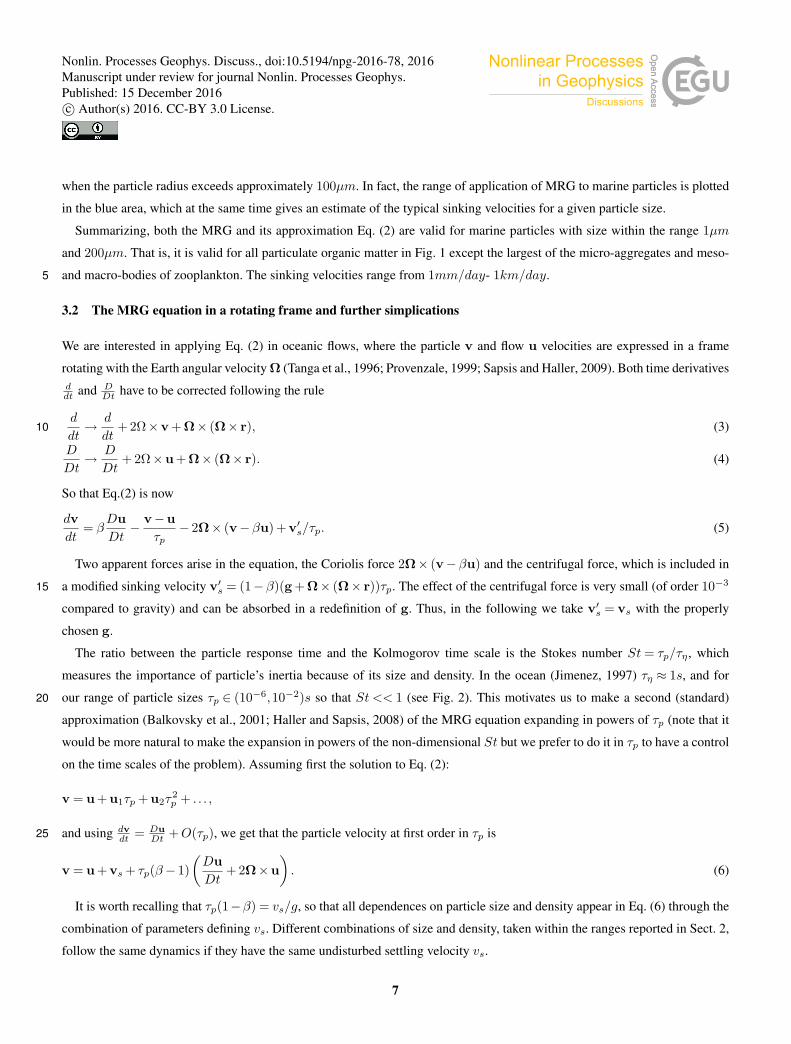
when the particle radius exceeds approximately 100µm. In fact, the range of application of MRG to marine particles is plotted

in the blue area, which at the same time gives an estimate of the typical sinking velocities for a given particle size.

Summarizing, both the MRG and its approximation Eq. (2) are valid for marine particles with size within the range 1µm

and 200µm. That is, it is valid for all particulate organic matter in Fig. 1 except the largest of the micro-aggregates and meso-

and macro-bodies of zooplankton. The sinking velocities range from 1mm/day- 1km/day.5

3.2 The MRG equation in a rotating frame and further simplications

We are interested in applying Eq. (2) in oceanic flows, where the particle v and flow u velocities are expressed in a frame

rotating with the Earth angular velocity Ω (Tanga et al., 1996; Provenzale, 1999; Sapsis and Haller, 2009). Both time derivativesddt and D

Dt have to be corrected following the rule

d

dt→ d

dt+ 2Ω×v + Ω× (Ω× r), (3)10

D

Dt→ D

Dt+ 2Ω×u + Ω× (Ω× r). (4)

So that Eq.(2) is now

dvdt

= βDuDt− v−u

τp− 2Ω× (v−βu) + v′s/τp. (5)

Two apparent forces arise in the equation, the Coriolis force 2Ω× (v−βu) and the centrifugal force, which is included in

a modified sinking velocity v′s = (1−β)(g + Ω× (Ω× r))τp. The effect of the centrifugal force is very small (of order 10−315

compared to gravity) and can be absorbed in a redefinition of g. Thus, in the following we take v′s = vs with the properly

chosen g.

The ratio between the particle response time and the Kolmogorov time scale is the Stokes number St= τp/τη , which

measures the importance of particle’s inertia because of its size and density. In the ocean (Jimenez, 1997) τη ≈ 1s, and for

our range of particle sizes τp ∈ (10−6,10−2)s so that St << 1 (see Fig. 2). This motivates us to make a second (standard)20

approximation (Balkovsky et al., 2001; Haller and Sapsis, 2008) of the MRG equation expanding in powers of τp (note that it

would be more natural to make the expansion in powers of the non-dimensional St but we prefer to do it in τp to have a control

on the time scales of the problem). Assuming first the solution to Eq. (2):

v = u + u1τp + u2τ2p + . . . ,

and using dvdt = Du

Dt +O(τp), we get that the particle velocity at first order in τp is25

v = u + vs + τp(β− 1)(DuDt

+ 2Ω×u). (6)

It is worth recalling that τp(1−β) = vs/g, so that all dependences on particle size and density appear in Eq. (6) through the

combination of parameters defining vs. Different combinations of size and density, taken within the ranges reported in Sect. 2,

follow the same dynamics if they have the same undisturbed settling velocity vs.

7


V s(m/s)

Size

0.5<β<0.99β=0.99β=0.50Rep>1τp>1s10-810-710-610-510-410-310-210-1100101

1μm 10μm 100μm 1mm 1cm 10cm

10 m/day100 m/day1000 m/dayKolmog

orov lentgthsca

le

Figure 2. Sinking velocity versus particle radius for different β, which is determined by densities. The blue zone determines the values of

the settling velocities at a given radius, as determined by the typical marine particle densities. The green area is determined by the condition

Rep > 1 for which the MRG equation is not valid. Use of the MRG equation is also unjustified for particles larger than the Kolmogorov

length scale also plotted in the figure. We also show the region τp > τη ≈ 1s where the additional approximation leading to Eq. (6) becomes

invalid.

A further discussion of Eq. (6) follows. At this order only three physical processes correct the particle velocity with respect

to the fluid velocity: the Stokes friction determining the settling velocity vs, the inertial term given by τp(β− 1)DuDt whose

major effect is to introduce a centrifugal force pulling particles away from vortex cores (Maxey, 1987; Michaelides, 1997),

and the influence of the Coriolis force 2τp(β− 1)Ω×u. Concerning sinking dynamics, the v = u + vs is the most relevant

8


approximation, and some studies, mainly in oceanographic contexts (Siegel and Deuser, 1997), considered it. Note that we

can use the right-hand-side of Eq. (6) with u = u(r, t) to define the particle velocity v as a velocity field in three-dimensional

space v = v(r, t). If one uses the lowest-order approximation v ≈ u we have ∇ ·v =∇ ·u = 0 when the fluid velocity field

u is incompressible (which is the case for ocean flows). This means that with only this term one cannot obtain a compressible

particle velocity which is the main reason quoted to explain why finite-size particles tend to cluster (Squires and Eaton, 1991;5

Bec, 2003). For this reason, numerous studies (Tanga et al., 1996; Michaelides, 1997; Bec et al., 2007; Cartwright et al.,

2010; Guseva et al., 2013; Beron-Vera et al., 2015) consider the role of the additional terms. With them ∇ ·v = τp(β− 1)∇ ·(DuDt +2Ω×u) 6= 0, and inertia-induced clustering may ocur. In the following sections we address two main questions: a) how

relevant for the sinking dynamics are the Coriolis and centrifugal terms?; and b) are they essential ingredients for the clustering

of biogenic particles? We will study the relevance of the different terms in Eq. (6) in a realistic oceanic setting.10

4 Numerical simulations

For the velocity flow u we use the outputs of a ROMS (Regional Ocean Modelling System) simulation of the Benguela region.

ROMS is a hydrostatic primitive equation model with free surface. We force it with climatological data in the region (Gutknecht

et al., 2013). The simulation area extends from 12S to 35S and from 4E to 19E (blue rectangle in Fig. 3). The velocity

field data set consists of 2 years of daily averages of zonal (u), meridional (v) and vertical velocity (w) components, stored in15

a 3D grid with a horizontal resolution of 1/12o and 32 vertical terrain-following levels using a stretched vertical coordinate

where the layer thickness increases from surface/bottom to the ocean interior.

In order to integrate particle trajectories from the velocity in Eq. (6) we interpolate linearly u(r, t) from the closest space-time

grid points to the actual particle locations. Given the huge disparity between the model resolution and the small particle-sizes

considered, it is pertinent to parameterize in some way the unresolved scales. This is done by adding a simple white noise to20

the particle velocity (Tang et al., 2012), with different intensity in the vertical and horizontal directions. Thus, we consider this

noisy version of the simplified MRG:

dr(t)dt

= v(t) (7)

v = u + vs + τp(β− 1)(DuDt

+ 2Ω×u)

+ W. (8)

W(t)≡√2DhWh(t) +√

2DvWz(t), with (Wh,Wz) = (Wx(t),Wy(t),Wz(t)) a three-dimensional vector Gaussian white25

noise with zero mean and correlations 〈Wi(t)Wj(t′)〉= δijδ(t− t′), i, j = x,y,z. We consider an horizontal eddy diffusivity,

Dh, depending on resolution length scale l according to Okubo formula (Okubo, 1971; Hernandez-Carrasco et al., 2011):

Dh(l) = 2.055× 104l1.55 (m2/s). Thus, if taking l ∼ 8 km= 8000 m (corresponding to 1/12) we obtain 10m2/s. In the

vertical direction we use a constant value of Dv = 10−5m2/s (Rossi et al., 2013).

9


Latitude

Longitude-36-34-32-30-28-26-24-22-20-18-16-14-12

4 6 8 10 12 14 16 18 20

Latitude

Longitude-36-34-32-30-28-26-24-22-20-18-16-14-12

4 6 8 10 12 14 16 18 20 -5000-4500-4000-3500-3000-2500-2000-1500-1000-5000

Bathymetry (m)

Figure 3. Map of region of study. Color corresponds to bathymetry. Blue rectangle is region used for simulations of the ROMS model.

Orange rectangle is the region for the clustering numerical experiment of Sect. 5 and red rectangle is the release site of the sinking numerical

experiments of Sect. 4.

10


In order to obtain quantitative assessment of the relative effects of the different physical terms in Eq. (8), we will compare

trajectories obtained from the following expressions which only consider some of the terms of the full expression Eq. (8):

v(0) = u + vs + W, (9)

v(co) = u + vs + τp(β− 1)2Ω×u + W, (10)

v(in) = u + vs + τp(β− 1)DuDt

+ W. (11)5

Besides the random noise term, the first expression (9) only considers the settling velocity, equation (10) resolves the settling

velocity plus the Coriolis effect, and equation (11) considers the settling plus the inertial term.

For the numerical experiments we will consider a set of six values of vs ranging from 5m/day to 200m/day, with different

integration times to have in all the cases a sinking to about 1000−1100 m depth. The stochastic equation (7) with expressions

(8)-(11) is written in spherical coordinates and numerically integrated by using a second-order Heun’s method with time step10

of 4 hours (Toral and Colet, 2014). We use R= 6371 km for the Earth radius, g = 9.81m/s2, and the angular velocity Ω

is a vector pointing in the direction of Earth axis and modulus |Ω|= 7.2722× 10−5 s−1. We use as initial starting date 17

September 2008. The numerical experiments consist in launching N = 6000 particles from initial conditions randomly chosen

in a square of size 1/6 centered at 10.0E 29.12S and −100.0m depth (red rectangle in Fig. 3), and let them to evolve for a

given time tf following Eq. (7) with expressions (8)-(11) using in each case identical initial conditions and the same sequence15

of random numbers for the noise terms. In this way we obtain the final positions of all the particles for each approximation to

the dynamics: ri(tf ), r(0)i (tf ), r(co)

i (tf ), and r(in)i (tf ), i= 1, ...,N .

Table 2 gives the mean and the standard deviation of the depths attained by the set of particles in each numerical experiment

as obtained from Eqs. (7) and (8). A first result is that the use of the different approximations (9)-(11) gives virtually the

same results. The only differences larger than 1 cm in mean or standard deviation are the ones for the smallest unperturbed20

settling velocity considered, vs = 5m/s, and are also reported in Table 2. The measured differences are negligible as compared

with the traveled distance or even with the model grid size. Indeed small changes in the ROMS model configuration or in the

velocity interpolation procedure would have an impact larger than this. The mean displacements in the horizontal obtained with

the different approximations are also within a 0.1% range. We thus conclude that the simplest approximation Eq. (9) which

only considers passive transport and an added constant sinking velocity already provides a good description of the sinking25

process for the type of marine particles considered here. As a side note, we comment that the depth attained by the particles

is always slightly shallower than z =−1100, which is the depth that would be reached in a still fluid. It is still debated under

which conditions fluid flows enhances or reduces the settling velocity (Maxey, 1987; Wang and Maxey, 1993; Ruiz et al., 2004;

Bec et al., 2014)

We perform now a more stringent test going beyond the analyses of mean displacements by considering differences between30

individual particle trajectories. To assess the impact of the Coriolis and of the inertial effects we compare the final positions

r(co)i (tf ), and r(in)

i (tf ) with the simpler dynamics Eq. (9) which gives r(0)i (tf ). To do so we compute the average absolute

11


vs integration time Mean final depth std final depth

(m/day) (days) (m) (m)

200 5 -1091.78 3.88

100 10 -1065.33 6.57

50 20 -1033.97 6.22

20 50 -1051.85 22.67

10 100 -1043.49 51.22

5 200 -1054.97 62.03

-1054.76 (co) 62.14

-1054.76 (in) 62.16

-1054.72 (0) 62.14Table 2. Mean and standard deviation of the set of depths attained, according to Eqs. (7) and (8), by the set of particles released from the red

rectangle in Fig. 3 at z =−100 for the different values of vs and integration times used. The results labeled (co), (in), and (0) are obtained

from the different approximations in Eqs. (9)-(11), which differ more than 1 cm from the ones obtained from Eq. (8) only in the vs = 5m/s

case.

difference in position per particle, which we separate in vertical and horizontal components:

r(k)h =

1N

N∑

i=1

∣∣∣x(0)i (tf )−x(k)

i (tf )∣∣∣ (12)

r(k)v =1N

N∑

i=1

∣∣∣z(0)i (tf )− z(k)

i (tf )∣∣∣ (13)

with xi = (xi,yi), and the superindex (k) takes the values (co) or (in).

Fig. 4 displays the influence of the inertial term as a function of the settling velocity. Certainly, the differences (both in5

vertical and horizontal) are negligible, being smaller than 1 m, which has to be compared with typical displacements in the

horizontal of hundreds of km and of 1000 m in the vertical. The conclusion is that this term can be neglected. Seemingly,

in Fig.5 the same type of comparison is done for the particle positions obtained with the Coriolis term. The differences with

respect to r(0)i are now higher (a maximum value of r ≈ 1000m in the horizontal and 10 cm in the vertical), but anyway they

are also negligible with respect to the total displacements or even with respect to the grid sizes. The trajectories of the full10

dynamics ruled by Eq. (8) are nearly identical to the ones under the approximation which keeps only the sinking term and

Coriolis, so that the corresponding comparison to r(0)i gives a figure essentially identical to Fig. 5 and will not be displayed

here.

For the range of sizes and densities of the marine particles considered here, the sinking dynamics is essentially given by the

velocity v = u+vs, which has been the one used in some oceanographic studies (Siegel and Deuser, 1997; Siegel et al., 2008;15

Roullier et al., 2014). Note however that a new question arises: what is then the reason for the observed clustering of falling

12


10-710-610-510-410-310-210-1100101

10 100

rin h,v(m)

vs(m/s)

rhrv

Figure 4. Average absolute difference per particle in distance traveled according to the inertial approximation Eq. (11) and the simpler one

Eq. (9). Upper blue line, horizontal component r(in)h ; lower red line, vertical component r(in)

v . The error bars are the standard errors in these

averages.

particles (Logan and D.B., 1990; Buesseler et al., 2007; Mitchell et al., 2008)? The argument of the non-inertial dynamics of

the particles does not serve since∇ ·v =∇ ·u = 0. A possible response is explored in the next section.

5 Geometric clustering of particles

Compressibility of the particle-velocity field, i.e.∇·v 6= 0, which can arise from inertial effects even when the corresponding

fluid-velocity field is incompressible∇·u = 0, has been identified as one of the mechanisms leading to preferential clustering5

of particles in flows (Squires and Eaton, 1991; Balkovsky et al., 2001). This is so because ρ(t), the particle density at time t at

the location r = r(r0, t) of a particle that started at r0 at time zero, satisfies ρ(t) = ρ(0)δ−1, where δ is a dilation factor equal

13


10-510-410-310-210-1100101102103

10 100

rco h,v(m)

vs(m/s)

rhrv

Figure 5. Average absolute difference per particle in distance traveled according to the Coriolis approximation Eq. (10) and the simpler one

Eq. (9). Upper blue line, horizontal component r(co)h ; lower red line, vertical component r(co)v . The error bars are the standard errors in these

averages.

to the determinant of the Jacobian | ∂r∂r0|, which satisfies

1δ

Dδ

Dt=∇ ·v (14)

or, using δ(0) = 1:

δ(tf ) = e∫ tf0 dt∇·v . (15)

Thus, particles will accumulate (i.e. higher ρ(tf )) in locations at which the arriving trajectories have passed predominantly5

through regions with ∇ ·v < 0. We have seen however that, to a good approximation ∇ ·v ≈∇ ·u = 0 since inertial effects

can be neglected for the type of marine particles we consider here, and then the three-dimensional particle-velocity field is

incompressible.

14


We now reproduce numerically a typical situation in which clustering of marine particles is observed. We release particles

uniformly in an horizontal layer close to the surface, letting them to sink in the presence of the oceanic flow, and observe the

distribution of the locations where they touch another horizontal deeper layer. The domain chosen is the rectangle 12S to 35S

and 4E to 19E (orange rectangle in Fig. 3). We divide the domain horizontally in squares of side 1/25, then initialize 1000

particles at random positions in each of them in August 20, 2008 at depth z =−100 m, and then integrate each trajectory until5

it reaches −1000m depth. We use expression (9) for the velocity, with vs = 50m/day. In order to avoid any small fluctuating

compressibility arising from the noise term we put W = 0 but we have checked that the result in the presence of noise is

virtually indistinguishable. At the bottom layer (z =−1000m) we count how many particles arrive to each of the 1/25 boxes

and display the result in Fig. 6(a). Despite ∇ ·v = 0 we see clear preferential clustering of particles in some regions related to

eddies and filaments. We note that our horizontal boxes have a latitude-dependent area so that distributing particles at random10

in them produces a latitude-dependent initial density which could lead to some final inhomogeneities. But we have checked

that for the range of displacements of the particles, this effect is everywhere smaller than 5% and thus can not be responsible

for the large clustering observed in Fig. 6(a). Nevertheless, this effect will be taken into account later.

We explain the observed particle clustering by noticing that what is measured in Fig. 6(a) is a projection in two dimensions

of a density field (the cloud of sinking particles) which evolves in three-dimensions. Even if the three-dimensional divergence15

is zero, and then an homogeneous three-dimensional density will remain homogeneous, a two-dimensional cut or projection

can be strongly inhomogeneous. This mechanism has been proposed to explain clustering and inhomogeneities in the ocean

surface (Huntley et al., 2015; Jacobs et al., 2016), but we show here that it is also relevant for the crossing of a horizontal layer

by a set of falling particles.

As a crude way to confirm that this clustering phenomenon arises from the two-dimensionality of the measurement, we20

estimate the changes in the horizontal density of evolving particle layers as if they were produced just by the horizontal part of

the velocity field. This is only correct if an initially horizontal particle layer remains always horizontal under evolution, which

is not true. But, given the huge differences in the values of the horizontal and vertical velocities in the ocean, we expect this

approximation to capture the essential physics and provide a qualitative explanation of the observed cluster. Thus we compute

the two-dimensional version of the dilation field, δh(x, tf ), at each horizontal location x in the deep layer at z =−1000m:25

δh(x, tf ) = e∫ tf0 dt∇h·v (16)

with the horizontal divergence

∇h ·v ≡∂vx∂x

+∂vy∂y

=∂u

∂x+∂v

∂y=−∂w

∂z, (17)

where in the second equality we have used Eq. (9) from which∇h ·v =∇h ·u and the third one is a consequence of∇·u = 0.

In order to get the values of δh on a uniform grid on the −1000m depth layer at the arrival date tf of the particles in the30

previous simulation, we integrate backwards in time trajectories from grid points separated 1/50 at z =−1000m until they

reach −100m. The starting date (tf ) of the backwards integration was September 7, 2008, i.e. 18 days after the release date

used in the previous clustering experiment. This value correspond to the average duration time of trajectories in that experiment.

Then δh was computed integrating in time the values of∇h ·v along every trajectory using Eq. (16).

15


Latitude

Longitude-38-36-34-32-30-28-26-24-22-20-18

6 8 10 12 14 16

Latitude

Longitude-38-36-34-32-30-28-26-24-22-20-18

6 8 10 12 14 16

Latitude

Longitude-38-36-34-32-30-28-26-24-22-20-18

6 8 10 12 14 16 00.20.40.60.811.21.41.61.82

Latitude

Longitude-38-36-34-32-30-28-26-24-22-20-18

6 8 10 12 14 16 0.80.840.880.920.9611.041.081.121.161.2a) b)

Figure 6. Results of the clustering numerical experiments of Sect. 5. a) Nf/N0, the number of particles Nf arriving to an horizontal box of

size 1/25 in the horizontal layer at z =−1000m, normalized by the number of particles N0 = 1000 released from the upper z =−100m

layer. b) The corrected dilation factor δ(x, tf )−1 cos(θf )/cos(θ0) mapped on the final z =−1000 m layer. It gives the ratio between

horizontal densities at the final and initial locations, corrected with the latitudinal dependence of the horizontal boxes used in panel a), to

give an estimation of the local particle number ratio between lower and upper layer.

Figure 6(b) displays the quantity δ(x, tf )−1 cos(θf )/cos(θ0), which gives the ratio between densities in the upper and lower

layer, corrected with the angular factors controlling the area of the horizontal boxes so that this can be compared with the

ratio between particle numbers displayed in Fig. 6(a). θf is the latitude of point x, and θ0 is the latitude of the corresponding

trajectory in the upper z =−100 m layer. As stated before, the latitudinal corrections by the cosine terms are always smaller

than a 5%. Although there is no perfect quantitative agreement, there is clear correspondence between the main clustered5

structures in panels (a) and (b) of Fig. 6, confirming that they originate from the horizontal dynamics in an incompressible

three-dimensional velocity field. We have checked in specific cases that locations with larger differences between Figs. 6(a)

and (b) correspond to places with large dispersion in the arrival times to the bottom layer, indicating deviations from the

horizontality assumption.

16


6 Conclusions

We have studied the problem of sinking particles in a realistic oceanic flow, focussing in the range of sizes and densities

appropriate for marine biogenic particles. Starting from a modeling approach in terms of the MRG equation (1), our conclusion

is that the simplest approximation given by Eq. (9), in which particles move passively except in the vertical direction in which

there is, together with the fluid flow, a constant settling velocity, is an accurate framework to describe the sinking process in the5

type of flows and particles considered. A re-assessment of these assumptions may be required if more complex processes (such

as aggregation/disaggregation) are included and when super-high resolution simulations of the ocean will become available.

Corrections arising from the Coriolis force turn out to be about 1000 times larger than the ones coming from inertial effects,

in agreement with the results in Sapsis and Haller (2009) or in Beron-Vera et al. (2015), but both of them are negligible when

compared to the effects of passive transport by the fluid velocity plus the added gravity term.10

If the fluid flow field u(r, t) has vanishing divergence then the same is true for the particle velocity field defined by the

approximation in Eq. (9). Then, no three-dimensional clustering can occur within this approximation. Nevertheless, we have

shown that two-dimensional cuts or projections of evolving three-dimensional particle clouds display horizontal clustering.

Competing interests. The authors declare that they have no conflict of interest.

Acknowledgements. We acknowledge support from Ministerio de Economía y Competitividad and Fondo Europeo de Desarrollo Regional15

through the LAOP project (CTM2015-66407-P, MINECO/FEDER), from the Office of Naval Research Grant No. N00014-16-1-2492, and

through a Juan de la Cierva Incorporación fellowship (IJCI-2014-22343) granted to V.R.

17


References

Azetsu-Scott, K. and Passow, U.: Ascending marine particles: Significance of transparent exopolymer particles (TEP) in the upper ocean,

Limnology and Oceanography, 49, 741–748, doi:10.4319/lo.2004.49.3.0741, 2004.

Balch, W. M., Bowler, B. C., Drapeau, D. T., Poulton, A. J., and Holligan, P. M.: Biominerals and the vertical flux of particulate organic

carbon from the surface ocean, Geophysical Research Letters, 37, L22 605, doi:10.1029/2010GL044640, 2010.5

Balkovsky, E., Falkovich, G., and Fouxon, A.: Intermittent Distribution of Inertial Particles in Turbulent Flows, Phys. Rev. Lett., 86, 2790–

2793, doi:10.1103/PhysRevLett.86.2790, 2001.

Bec, J.: Fractal clustering of inertial particles in random flows, Physics of Fluids, 15, 81–84, doi:10.1063/1.1612500, 2003.

Bec, J., Biferale, L., Cencini, M., Lanotte, A., Musacchio, S., and Toschi, F.: Heavy Particle Concentration in Turbulence at Dissipative and

Inertial Scales, Phys. Rev. Lett., 98, 084 502, doi:10.1103/PhysRevLett.98.084502, 2007.10

Bec, J., Homann, H., and Ray, S. S.: Gravity-Driven Enhancement of Heavy Particle Clustering in Turbulent Flow, Phys. Rev. Lett., 112,

184 501, doi:10.1103/PhysRevLett.112.184501, 2014.

Beron-Vera, F. J., Olascoaga, M. J., Haller, G., Farazmand, M., Triñanes, J., and Wang, Y.: Dissipative inertial transport patterns near coherent

Lagrangian eddies in the ocean, Chaos, 25, 087412, doi:10.1063/1.4928693, 2015.

Buesseler, K. O., Antia, A. N., Chen, M., Fowler, S. W., Gardner, W. D., Gustafsson, O., Harada, K., Michaels, A. F., Rutgers van der Loef,15

M., K., S. M. S. D., and Trull, T.: An assessment of the use of sediment traps for estimating upper ocean particle fluxes, Journal of Marine

Research, 65, 345–416, 2007.

Cartwright, J. H. E., Feudel, U., Károlyi, G., de Moura, A., Piro, O., and Tél, T.: Dynamics of Finite-Size Particles in Chaotic Fluid Flows,

pp. 51–87, Springer Berlin Heidelberg, Berlin, Heidelberg, doi:10.1007/978-3-642-04629-2_4, 2010.

Daitche, A. and Tél, T.: Memory Effects are Relevant for Chaotic Advection of Inertial Particles, Phys. Rev. Lett., 107, 244 501,20

doi:10.1103/PhysRevLett.107.244501, 2011.

De La Rocha, C. L. and Passow, U.: Factors influencing the sinking of POC and the efficiency of the biological carbon pump, Deep Sea

Research Part II: Topical Studies in Oceanography, 54, 639–658, doi:10.1016/j.dsr2.2007.01.004, 2007.

DeVries, T., F., P., and Deutsch, C.: The sequestration efficiency of the biological pump, Geophys. Res. Lett, 39, L13 601, 2012.

Falkovich, G. and Fouxon, I Stepanov, M. G.: Acceleration of rain initiation by cloud turbulence, Nature, 419, 151–154, 2002.25

Faxén, H.: Der Widerstand gegen die Bewegung einer starren Kugel in einer zähen Flüssigkeit, die zwischen zwei parallelen ebenen Wänden

eingeschlossen ist, Annalen der Physik, 373, 89–119, doi:10.1002/andp.19223731003, 1922.

Gatignol, R.: The Faxén formulae for a rigid particle in an unsteady non-uniform Stokes flow, J. Mec. Theor. Appl., 990, 143–160, 1983.

Guidi, L., Jackson, G., Stemmann, L., Miquel, J., Picheral, M., and Gorsky, G.: Relationship between particle size distribution and flux in

the mesopelagic zone, Deep-Sea Research I, 55, 1364–1374, 2008.30

Guseva, K., Feudel, U., and Tél, T.: Influence of the history force on inertial particle advection: Gravitational effects and horizontal diffusion,

Phys. Rev. E, 88, 042 909, doi:10.1103/PhysRevE.88.042909, 2013.

Gutknecht, E., Dadou, I., Le Vu, B., Cambon, G., Sudre, J., Garçon, V., Machu, E., Rixen, T., Kock, A., Flohr, A., Paulmier, A., and Lavik, G.:

Coupled physical/biogeochemical modeling including O2-dependent processes in the Eastern Boundary Upwelling Systems: application

in the Benguela, Biogeosciences, 10, 3559–3591, doi:10.5194/bg-10-3559-2013, 2013.35

Haller, G. and Sapsis, T.: Where do inertial particles go in fluid flows?, Physica D: Nonlinear Phenomena, 237, 573–583,

doi:10.1016/j.physd.2007.09.027, 2008.

18


Hedges, J. I.: Biogeochemistry of Marine Dissolved Organic Matter, Elsevier, doi:10.1016/B978-012323841-2/50003-8, 2002.

Henson, S., Sanders, R., and Madsen, E.: Global patterns in efficiency of particulate organic carbon export and transfer to the deep ocean,

Global Biogeochem. Cycles, 26, GB1028, 2012.

Hernandez-Carrasco, I., López, C., Hernández-García, E., and Turiel, A.: How reliable are Finite-Size Lyapunov Exponents for the assess-

ment of ocean dynamics?, Ocean Modelling, 36, 208–218, doi:10.1016/j.ocemod.2010.12.006, 2011.5

Huntley, H. S., Lipphardt, B. L., Jacobs, G., and Kirwan, A. D.: Clusters, deformation, and dilation: Diagnostics for material accumulation re-

gions, Journal of Geophysical Research: Oceans, 120, 6622–6636, doi:10.1002/2015JC011036, http://dx.doi.org/10.1002/2015JC011036,

2015.

Jackson, G. A.: Effect of coagulation on a model planktonic food web, Deep Sea Research Part I: Oceanographic Research Papers, 48,

95–123, doi:10.1016/S0967-0637(00)00040-6, 2001.10

Jacobs, G. A., Huntley, H. S., Kirwan, A. D., Lipphardt, B. L., Campbell, T., Smith, T., Edwards, K., and Bartels, B.: Ocean processes

underlying surface clustering, Journal of Geophysical Research: Oceans, 121, 180–197, doi:10.1002/2015JC011140, 2016.

Jimenez, J.: Ocean turbulence at milimiter scales, Scientia Marina, 61, 47–56, 1997.

Komar, P. D., Morse, A. P., Small, L. F., and Fowler, S. W.: An analysis of sinking rates of natural copepod and euphausiid fecal pellets,

Limnology and Oceanography, 26, 172–180, doi:10.4319/lo.1981.26.1.0172, 1981.15

Logan, B. and D.B., W.: Fractal geometry of marine snow and other biological aggregates, Limnology and Oceanography, 35,

doi:10.4319/lo.1990.35.1.0130, 1990.

Maggi, F.: The settling velocity of mineral, biomineral, and biological particles and aggregates in water, Journal of Geophysical Research:

Oceans, 118, 2118–2132, doi:10.1002/jgrc.20086, 2013.

Maggi, F. and Tang, F. H.: Analysis of the effect of organic matter content on the architecture and sinking of sediment aggregates, Marine20

Geology, 363, 102–111, doi:10.1016/j.margeo.2015.01.017, 2015.

Maxey, M. R.: The gravitational settling of aerosol particles in homogeneous turbulence and random flow fields, Journal of Fluid Mechanics,

174, 441–465, doi:10.1017/S0022112087000193, 1987.

Maxey, M. R. and Riley, J. J.: Equation of motion for a small rigid sphere in a nonuniform flow, Physics of Fluids, 26, 883–889,

doi:10.1063/1.864230, 1983.25

McDonnell, A. M. P. and Buesseler, K. O.: Variability in the average sinking velocity of marine particles, Limnology and Oceanography, 55,

2085–2096, doi:10.4319/lo.2010.55.5.2085, 2010.

Michaelides, E. E.: Hydrodynamic Force and Heat/Mass Transfer From Particles, Bubbles, and Drops, Journal of Fluids Engineering, 125,

209–238, doi:10.1115/1.1537258, 1997.

Mitchell, J., H., Y., Seuront, L., Wolk, F., and Li, H.: Phytoplankton patch patterns: Seascape anatomy in a turbulent ocean, Journal of Marine30

Systems, 69, 247–253, 2008.

Moore, J. and Villareal, T.: Size-ascent rate relationships in positively buoyant marine diatoms., Limnology and Oceanography, 41, 1996.

Okubo, A.: Oceanic diffusion diagram, Deep-Sea Research, 18, 789–802, 1971.

Provenzale, A.: Transport by coherent barotropic vortices, Annual Review of Fluid Mechanics, 31, 55–93, 1999.

Qiu, Z., Doglioli, A., and Carlotti, F.: Using a Lagrangian model to estimate source regions of particles in sediment traps, Science China:35

Earth Sciences, 57, 2447–2456, doi:10.1007/s11430-014-4880-x, 2014.

Rossi, V., Van Sebille, E., Sen Gupta, E., Garçon, V., and England, M.: Multi-decadal projections of the surface and interior pathways of the

Fukushima Cesium-137 radioactive plume, Deep Sea-Research I, 80, 37–46, 2013.

19


Roullier, F., Berline, L., Guidi, L., Durrieu De Madron, X., Picheral, M., Sciandra, A., Pesant, S., and Stemmann, L.: Particle size distribution

and estimated carbon flux across the Arabian Sea oxygen minimum zone, Biogeosciences, 11, 4541–4557, doi:10.5194/bg-11-4541-2014,

2014.

Ruiz, J., Macias, D., and Peters, F.: Turbulence increases the average settling velocity of phytoplankton cells, Proceedings of the National

Academy of Sciences, 101, 17 720–17 724, 2004.5

Sabine, C., Feely, R., Gruber, N., Key, R., Lee, K., Bullister, J., Wanninkhof, R., Wong, C., Wallace, D., Tilbrook, B., Millero, F., Peng, T.,

Kozyr, A., Ono, T., and Rios, A.: The Oceanic Sink for Anthropogenic CO2, Science, 305, 367–371, 2004.

Sapsis, T. and Haller, G.: Inertial Particle Dynamics in a Hurricane, Journal of the Atmospheric Sciences, 66, 2481–2492,

doi:10.1175/2009JAS2865.1, 2009.

Siegel, D., Fields, E., and Buesseler, K. O.: A bottom-up view of the biological pump: Modeling source funnels above ocean sediment traps,10

Deep-Sea Research I, 55, 108–127, 2008.

Siegel, D. A. and Deuser, W. G.: Trajectories of sinking particles in the Sargasso Sea: modeling of statistical funnels above deep-ocean

sediment traps, Deep-Sea Research Part I-Oceanographic Research Papers, 44, 1519 – 1541, 1997.

Simon, M., Grossart, H., Schweitzer, B., and Ploug, H.: Microbial ecology of organic aggregates in aquatic ecosystems, Aquatic Microbial

Ecology, 28, 175–211, doi:10.3354/ame028175, 2002.15

Squires, K. D. and Eaton, J. K.: Preferential concentration of particles by turbulence, Physics of Fluids A, 3, 1169–1178, 1991.

Stemmann, L. and Boss, E.: Plankton and particle size and packaging: from determining optical properties to driving the biological pump.,

Annual Review of Marine Science, 4, 263–90, doi:10.1146/annurev-marine-120710-100853, 2012.

Tang, W., Knutson, B., Mahalov, A., and Dimitrova, R.: The geometry of inertial particle mixing in urban flows, from deterministic and

random displacement models, Physics of Fluids, 24, doi:10.1063/1.4729453, 2012.20

Tanga, P., Babiano, A., Dubrulle, B., and Provenzale, A.: Forming Planetesimals in Vortices, Icarus, 121, 158–170,

doi:10.1006/icar.1996.0076, 1996.

Toral, R. and Colet, P.: Stochastic numerical methods: an introduction for students and scientists, John Wiley & Sons, 2014.

van Sebille, E., Scussolini, P., Durgadoo, J., Peeters, F., Biastoch, A., Weijer, W., Turney, C. S. M., Paris, C. B., and Zahn, R.: Ocean currents

generate large footprints in marine palaeoclimate proxies, Nature communications, 6, 6521, doi:10.1038/ncomms7521, 2015.25

Wang, L. and Maxey, M. R.: Settling velocity and concentration distribution of heavy particles in homogeneous isotropic turbulence, Journal

of Fluid Mechanics, 256, 27–68, 1993.

20


Modeling the dynamical sinking of biogenic particles in ...

Documents

Transcript of Modeling the dynamical sinking of biogenic particles in ...