
MODELING OF POPULATION DISTRIBUTION IN SPACE AND TIME … · applied to the PhD program at the ITC...
192
MODELING OF POPULATION DISTRIBUTION IN SPACE AND TIME TO SUPPORT DISASTER RISK MANAGEMENT Sérgio M. C. Freire
Transcript of MODELING OF POPULATION DISTRIBUTION IN SPACE AND TIME … · applied to the PhD program at the ITC...

MODELING OF POPULATION DISTRIBUTION IN SPACE AND TIME TO SUPPORT DISASTER RISK
MANAGEMENT
Sérgio M. C. Freire

3
MODELING OF POPULATION DISTRIBUTION IN SPACE AND TIME TO SUPPORT DISASTER RISK
MANAGEMENT
DISSERTATION
to obtain the degree of doctor at the University of Twente,
on the authority of the rector magnificus, prof.dr. T.T.M. Palstra,
on account of the decision of the Doctorate Board to be publicly defended
on Friday 8 May 2020 at 16.45 hours
by
Sérgio Manuel Carneiro Freire born on the 14th of May 1972
in Porto, Portugal

This dissertation has been approved by Prof. dr.ir. R.V. Sliuzas, supervisor
Prof. dr.ir. M.F.A.M. van Maarseveen, supervisor
ITC dissertation number 382 ITC, P.O. Box 217, 7500 AE Enschede, The Netherlands
ISBN 978-90-365- 4999-8 DOI 10.3990/1.9789036549998 Cover designed by Job Duim Printed by ITC Printing Department Copyright © 2020 by Sérgio Manuel Carneiro Freire, The Netherlands. All rights
reserved. No parts of this thesis may be reproduced, stored in a retrieval system or transmitted in any form or by any means without permission of the author. Alle rechten voorbehouden. Niets uit deze uitgave mag worden vermenigvuldigd, in enige vorm of op enige wijze, zonder voorafgaande schriftelijke toestemming van de auteur.

Graduation committee:
Chairman/Secretary Prof.dr. F.D. van der Meer Supervisor(s) Prof.dr.ir. R.V. Sliuzas
Prof.dr.ir. M.F.A.M. van Maarseveen
Members Prof.dr.ir. R.V. Sliuzas
Prof.dr.ir. M.F.A.M. van Maarseveen
Prof.dr. K. Pfeffer Prof.dr.ir. A. Stein dr. C.J. van Westen Prof. dr. C. Linard
Prof. dr. D. Martin

Dedicated to Sara and Marta:
“May you build a ladder to the stars
And climb on every rung
May you stay forever young”
Bob Dylan

i
Foreword It became a sort of tradition to equate a PhD to a ‘long and arduous journey’
– but it certainly was in this case. The work comprising this thesis spans 9
years, two countries and two research institutions where I have lived and
worked in this period: the FCSH-UNL (Lisbon, Portugal) and the EC-JRC (Ispra,
Italy).
My interest in modeling population distribution was born in the previous
millennium, during my time as graduate student at the University of Kansas
(USA). There on the edge of the Great Plains I had the fortune of being exposed
to the first version of LandScan global population grid (1998) and meeting its
visionary author, Jerry Dobson. I was struck by the apparent simplicity and
broad reach of the concept that characterize bright developments, and was
hooked on the possibilities.
After leaving KU I continued to develop my population models, and around
2008 I also directed my interest to their applications, especially in Disaster
Risk Management, as that seemed to me the domain where most societal
benefits were to be gained. I did this mostly on my own time while working on
other research projects and activities (e.g. teaching GIS), as I had no funding
for this specific line of research. I tried as much as possible to connect topics
and during those very productive years managed to develop several
applications of improved population distribution across different domains.
Having amassed some research experience and publications, around 2012 I
started inquiring about the possibility of turning some of this body of work and
publications into a PhD thesis, but this was deemed not viable. I moved on,
embracing a new challenge at the EC-JRC in Italy.
In 2015, with more than 100 scientific publications under my belt (and having
contributed to two PhDs) an opportunity appeared that could lead to earning
that degree that is a necessary (but not sufficient) step for a researcher to
improve his job prospects. Through Richard Sliuzas, whom I had met earlier, I
applied to the PhD program at the ITC Faculty, University of Twente (a perfect
fit for my topic), submitted a proposal, and formally enrolled in 2016. At this
point I assumed it would be rather straightforward to build a decent PhD thesis
as an external student by combining my ongoing research at JRC with that
already published.
I was wrong, of course – being with small children in a foreign country, having
a wife with frequent business travels, and an absorbing job, this was in
hindsight not a bright idea, and one that I regretted often. Paradoxically, a
truly smart person would have chosen otherwise than going for a PhD. This
diverted much energy, time, and patience from important activities and
persons, and represented a high cost for an unknown benefit. And yet here I

ii
am, nearing completion. In the process, I confirmed that earning a PhD is as
much a proof of research skills as it is a trial of endurance, resilience, and
stamina (the fact that many fail this test, enduring mental or physical damage,
would warrant more attention from those involved in awarding these degrees).
As I write this in Lombardy, we are in the middle of the COVID-19 pandemic,
which started just when I was in the home stretch of finalizing this thesis.
Besides prompting a worldwide lockdown and crisis without an end in sight
(and postponing my well-deserved vacation), this epidemic tragically
underlines the importance of disaster risk management and how much work
remains to improve it.

iii
Acknowledgements
Most of the publications comprising the core of this thesis have resulted from
international collaborations, and I am especially pleased and proud of this
circumstance. So I start by thanking all 12 co-authors, from seven nationalities
and four institutions in two continents – I was honored to have you on board.
Special thanks to my buddy and co-author extraordinaire Chris Aubrecht; my
initial solitary efforts at population modeling and applications had a boost when
we met at Gi4DM 2009 in Prague and joined interests and forces for a fruitful
collaboration and friendship that I deeply cherish. I am also appreciative of the
many people with whom I crossed paths and discussed ideas at numerous
scientific meetings (in four continents), many of whom I came to befriend.
Although this thesis features ’only’ five publications as core chapters, in two of
my lines of research merging here I have authored and co-authored 50+
scientific publications, of which 45 are cited in this thesis. Therefore I also want
to acknowledge that large group of co-authors, with whom I have learned so
much.
I want to thank the people and institutions who contributed data to the work
supporting this thesis, especially important when this research was unfunded:
António Costa, Francisco Costa, Albertina Lérias (Geopoint Lda.), José L.
Zêzere (RISKam group/CEG-IGOT), Nuno Gomes, and Lisbon Metropolitan
Area.
At FCSH-UNL in Lisbon I thank my colleagues from e-GEO and especially José
A. Tenedório and Carlos Pereira da Silva for supporting me in this line of
research when no one else was.
I thank my teammates at JRC, in particular Martino Pesaresi for the
encouragement and the enlightening discussions, but also my good comrades
of office 112: Aneta Florczyk, Marcello Schiavina, and Michele Melchiorri –
Michele, for assistance with the template and formatting, grazie mille.
I am grateful to ITC and my supervisors, Prof. Martin van Maarseveen and Prof.
Richard Sliuzas for accepting me as their student and for their supervision.
Richard, thanks so much for your guidance and generosity and apologies for
my impatience. I also express my gratitude to the distinguished PhD
Committee Members, in particular to the external members (Prof. Martin and
Prof. Linard) for accepting to serve on this jury. I extend my appreciation to
Petra Weber and ITC staff for all assistance.
To my former colleagues and life friends Hugo Carrão and António Nunes um
grande abraço for their ever-present encouragement. A special thank you is
due to Alex de Sherbinin for showing me that this could be done and that it
was not too late to do it.

iv
Last but certainly not least, I thank all my family and especially my wife Ana
for her support and for being so resilient during these last couple of tough
years for both of us. I owe a special recognition and apology to my daughters
Sara and Marta, who (while babies) kept me company during long nights while
I did much of the early work supporting this thesis. Then more recently, this
thesis was put together stealing also their time – and therefore it is dedicated
to them.

v
Table of Contents Foreword .............................................................................................. i Acknowledgements ............................................................................... iii List of Figures ..................................................................................... viii List of Tables ........................................................................................ x Acronyms and abbreviations .................................................................. xi Chapter 1. Introduction, context and objectives ........................................ 1
1.1. Introduction and Significance ........................................................ 2 1.2. Context and Background .............................................................. 3
1.2.1 Population exposure and risk landscape, governance, and trends . 3
1.2.2 Mapping exposure for assessing populations at risk .................... 7
1.2.3 Beyond exposure: the relevance of population in integrated DRM 13
1.2.4 Background: Modeling and mapping of population distribution in space and time (for exposure analysis and DRM) .............................. 17
1.3 Objectives and structure of the Dissertation ................................... 27 Chapter 2. Modeling of spatio-temporal distribution of urban population at
high-resolution – value for risk assessment and emergency management .. 37 2.1 Introduction ............................................................................... 38
2.1.1 Population distribution and emergency management ................. 38
2.1.2 Population in space and time .................................................. 39
2.2 Methods .................................................................................... 40 2.2.1 Study area ........................................................................... 41
2.2.2 Data sets ............................................................................. 42
2.2.3 Model .................................................................................. 43
2.3 Results ...................................................................................... 45 2.3.1 Verification and validation ...................................................... 45
2.4 Sample applications .................................................................... 46 2.4.1 Case study A: technological hazard (airborne toxic plume release) 46
2.4.2 Case study B: natural disaster (earthquake) ............................ 47
2.4.3 Case study C: terrorist attack (bombing of shopping center) ...... 48
2.4.4 Case study D: planning of best route for hazardous materials transportation .............................................................................. 49
2.5 Conclusions ............................................................................... 51 Chapter 3. Integrating population dynamics into mapping human exposure to
seismic hazard .................................................................................... 53 3.1 Introduction ............................................................................... 54
3.1.1 The importance of population dynamics for disaster risk assessment .................................................................................................. 54
3.1.2 Population exposure to seismic hazard .................................... 56

vi
3.2 Study area and data ................................................................... 57 3.2.1 Study area ........................................................................... 57
3.2.2 Data sets ............................................................................. 60
3.3 Methodology .............................................................................. 61 3.3.1 Modeling spatio-temporal population distribution ...................... 61
3.3.2 Assessing population and classifying human exposure to seismic hazard 63
3.4 Results and discussion ................................................................ 68 3.5 Conclusions ............................................................................... 70
Chapter 4. Advancing tsunami risk assessment by improving spatio-temporal
population exposure and evacuation modeling ........................................ 73 4.1 Introduction ............................................................................... 74 4.2 Data and study area ................................................................... 76
4.2.1 Study area ........................................................................... 76
4.2.2 Data sets ............................................................................. 78
4.3 Methodology .............................................................................. 79 4.3.1 Modeling nighttime and daytime population distribution ............ 79
4.3.2 Assessing population exposure to tsunami ............................... 81
4.3.3 Tsunami evacuation modeling ................................................ 81
4.4 Results and discussion ................................................................ 83 4.5 Conclusions and outlook .............................................................. 86
Chapter 5. Enhanced data and methods for improving open and free global
population grids: putting ‘leaving no one behind’ into practice .................. 89 5.1 Introduction .......................................................................... 90 5.2 Materials and methods ................................................................ 93
5.2.1 Data sets ............................................................................. 94
5.2.2. Revision of ‘unpopulated’ units .............................................. 95
5.2.3 Harmonization of population and settlement data along coastlines .................................................................................................. 97
5.3 Results and discussion ............................................................... 100 5.3.1 Revision of unpopulated units ............................................... 100
5.3.2 Harmonization of population and settlement data along coastlines ................................................................................................. 104
5.4 Conclusions .............................................................................. 107 Chapter 6. An Improved Global Analysis of Population Distribution in Proximity
to Active Volcanoes ............................................................................ 109 6.1 Introduction .............................................................................. 110
6.1.1 Potential Global Population Exposure to Volcanic Hazard —Narrowing Data Gaps ................................................................................... 112
6.1.2 The Contribution of the Global Human Settlement Layer (GHSL) to DRM ........................................................................................... 113
6.2 Materials and Methods ............................................................... 115

vii
6.2.1 Data .................................................................................. 115
6.2.2 Assessing Global Population Distribution and Volcanism ............ 117
6.3 Results and Discussion ............................................................... 118 6.3.1 Global Population Distribution from 1975 to 2015 in Relation to Volcanism ................................................................................... 118
6.3.2 Population Distribution from 1975 to 2015 in Relation to Volcanism, in Southeast Asia and Central America ........................................... 124
6.4 Conclusions .............................................................................. 131 Chapter 7. Synthesis, conclusions, and outlook ...................................... 133
7.1 Introduction .............................................................................. 134 7.2 Main results: Modeling population distribution in space and time to support Disaster Risk Management ................................................... 134
7.2.1 Chapter 2: Modeling of spatio-temporal distribution of urban
population at high-resolution – value for risk assessment and emergency management ............................................................................... 135
7.2.2 Chapter 3: Integrating population dynamics into mapping human exposure to seismic hazard ........................................................... 136
7.2.3 Chapter 4: Advancing tsunami risk assessment by improving spatio-
temporal population exposure and evacuation modeling ................... 138
7.2.4 Chapter 5: Enhanced data and methods for improving open and free
global population grids: putting ‘leaving no one behind’ into practice .. 140
7.2.5 Chapter 6: An Improved Global Analysis of Population Distribution in
Proximity to Active Volcanoes, 1975–2015 ...................................... 142
7.3 Other research contributions: cross-disciplinary benefits and applications
of the produced population distribution data for modelling, assessing
impacts, and measuring access to services and resources. ................... 144 7.4 Challenges and Way Forward ...................................................... 146
Bibliography ...................................................................................... 151 Summary .......................................................................................... 171 Samenvatting .................................................................................... 173
viii
List of Figures Figure 1 A typology of hazards and respective characteristics. Source: UNEP/GRID Arendal (http://maps.grida.no/go/graphic/typology_of_hazards).
........................................................................................................ 12 Figure 2 DRM process and phases, conceptualized as cycle and spiral. Source: Aubrecht et al. 2013 ............................................................................ 14 Figure 3 Location of the study area in Portugal and in the Lisbon Metro Area (LMA) (Source: CAOP). ........................................................................ 42 Figure 4 Flowchart of main tasks involved in the model: input data are noted in light gray, secondary products in orange, and main results noted in bold and
red .................................................................................................... 44 Figure 5 Case study A: airborne toxic plume release in Oeiras (Source: IGP; TeleAtlas). ......................................................................................... 47 Figure 6 Case study B: earthquake affecting downtown Cascais (Source: IGP; TeleAtlas). ......................................................................................... 48 Figure 7 Case study C: terrorist attack in a Cascais shopping center (Source:
IGP; TeleAtlas). .................................................................................. 49 Figure 8 Case study D: best route considering the population distribution (Source: IGP; TeleAtlas). ..................................................................... 50 Figure 9 Study area - Lisbon Metropolitan Area (LMA) ............................. 58 Figure 10 Seismic Intensity map for the study area (background from Google Earth). ............................................................................................... 60 Figure 11 Nighttime population density and seismic zones (background from
Google Earth). .................................................................................... 64 Figure 12 Daytime population density and seismic zones (background from Google Earth). .................................................................................... 64 Figure 13 Classification approach to categorize human exposure levels ...... 65 Figure 14 Map of nighttime human exposure to seismic hazard ................. 67 Figure 15 Map of daytime human exposure to seismic hazard ................... 67 Figure 16 Study area – Lisbon Metropolitan Area (LMA) ........................... 77 Figure 17 Tsunami Inundation Susceptibility map for the LMA (background from Google Earth) ............................................................................. 78 Figure 18 Nighttime (A) and daytime (B) population density and Tsunami Inundation Susceptibility zones (background from Google Earth) .............. 81 Figure 19 Study area for Tsunami evacuation modeling ........................... 82 Figure 20 Nighttime (A) and daytime (B) Tsunami evacuation modeling ..... 85 Figure 21 Flow chart of the ‘split and merge’ approach ............................ 97 Figure 22 Examples of detected discrepancies (patches larger than 1 km2) between GPWv4 (blue line) and GHS-BUILT 2014 (orange) along the coasts of (A) Japan (JPN), (B) Tunisia (TUN), (C) China (CHN), and (D) Romania (ROU) ........................................................................................................ 99 Figure 23 Global distribution of census units without population in GPWv4.10 data and those flagged based on the automated procedure developed (USA not
considered). Note that existence of unpopulated units is merely a feature of census design and not of the landscape ................................................ 100 Figure 24 Examples of application of the ‘split and merge’ approach to census units incorrectly deemed as unpopulated in (A) Guyana and (B) Lebanon, before (1) and after (2) the procedure is applied. Orange filling and red dashed boundary represent the original problematic polygon; blue solid line delineates
ix
borders of upper administrative level; grey solid polygons are correctly declared unpopulated polygons; solid coloured areas are the resulting
polygons; areas outside the processed administrative unit are shaded. ..... 102 Figure 25 Illustration of resulting 250-m population grids for 2015 in (A) Guyana and (B) Lebanon .................................................................... 104 Figure 26 Visually confirmed coastline discrepancy patches larger than 1 km2. ....................................................................................................... 105 Figure 27 Example illustrating situation (A) before and (B) after manual harmonization of a stretch of Caspian Sea coastline in Russia. Solid black lines
enclose original census units; black pixels denote mapped built-up areas (shaded: already within census boundaries; solid: outside original census areas). ............................................................................................. 105 Figure 28 Example of automated approach to mitigate inconsistencies along the coastline of Ukraine. This example shows the generation of a 2-km buffer that was split using the ‘split and merge’ approach. Solid black lines enclose original census units; solid blue line represents the extended boundary into the
sea through 2-km buffer; solid red lines represent the splitting of buffer into parts assigned to the nearest neighbouring unit; black pixels represent mapped built-up areas (shaded: already within census boundaries; solid: outside original census areas). ........................................................................ 106 Figure 29 Distribution of the two global datasets of volcanoes used in this study: Holocene Volcano List v4.7.6 (HV) and Significant Volcanic Eruption
Database (SV) (World Mollweide projection). ......................................... 117 Figure 30 Cumulative population as a function of radial distance to Holocene volcanoes (HV), in 1975, 1990, 2000, and 2015. ................................... 121 Figure 31 Cumulative population as a function of radial distance to volcanoes in Significant Volcanic Eruption Database (SV), in 1975, 1990, 2000, and 2015. ....................................................................................................... 121 Figure 32 Average population density as a function of radial distance to
Holocene volcanoes (HV), in 1975, 1990, 2000, and 2015. ...................... 122 Figure 33 Average population density as a function of radial distance to volcanoes in Significant Volcanic Eruption Database (SV), in 1975, 1990, 2000, and 2015. ......................................................................................... 122 Figure 34 Selected distances from Holocene volcanoes in (A) Southeast Asia and (B) Central America. .................................................................... 125 Figure 35 Average population density in Southeast Asia (SEAsia) and Central
America (CAm) as a function of radial distance of Holocene Volcanoes (HV), in 1975 and 2015. ................................................................................. 129 Figure 36 Average population density in Southeast Asia (SEAsia) and Central America (CAm) as a function of radial distance of volcanoes in Significant Volcanic Eruption Database (SV), in 1975 and 2015. .............................. 129 Figure 37 Island of Java (Indonesia), showing selected distances from Holocene
volcanoes, main cities, and population distribution in 2015 from GHS-POP (World Mollweide projection). .............................................................. 130

x
List of Tables
Table 1 Usefulness of geospatial demographic data (with focus on total population counts and density) in DRM phases. Source: author own elaboration
........................................................................................................ 15 Table 2 Overview of Chapters in this Thesis ............................................ 28 Table 3 Main characteristics of chapters in this thesis in relation to main research topics and concepts; main innovative aspects highlighted in bold . 34 Table 4 (cont.) Main characteristics of chapters in this thesis in relation to main research topics and concepts; main innovative aspects highlighted in bold . 35 Table 5 Main input datasets used for modeling nighttime and daytime
population .......................................................................................... 43 Table 6 Total exposed population in each case study ............................... 49 Table 7 Total exposed population along each route and period .................. 50 Table 8 Nighttime and daytime population in the municipalities of the Lisbon Metropolitan Area, in 2001 (derived from INE, 2001, 2003) ..................... 59 Table 9 Main input data sets used for modeling population distribution ...... 61 Table 10 Population exposed to seismic intensity levels in nighttime and daytime periods in the study area ......................................................... 69 Table 11 Total surface and population in each human exposure class in nighttime and daytime periods in the study area ..................................... 69 Table 12 Main input data sets used for modeling population distribution .... 79 Table 13 Population exposed to Tsunami inundation levels in nighttime and daytime periods in the LMA .................................................................. 84 Table 14 Population remaining in hazard zone and successful evacuees after different time intervals of tsunami evacuation ........................................ 85 Table 15 List of countries in which problematic polygons were selected ..... 101 Table 16 Population (in millions and as percentage of World total) by radial distance from Holocene volcanoes (HV) in 1975, 1990, 2000, and 2015. .. 119 Table 17 Compound annual growth rate of population by radial distance from Holocene volcanoes (HV) for each time interval. .................................... 119 Table 18 Population (in millions and percentage of World total) by radial distance from volcanoes with significant eruptions (SV) in 1975, 1990, 2000, and 2015. ......................................................................................... 119 Table 19 Compound annual growth rate of population by radial distance of volcanoes with significant eruptions (SV) for each time interval. .............. 120 Table 20 Population (in millions and percentage of region total) by radial
distance of Holocene volcanoes (HV) and volcanoes in Significant Volcanic Eruption Database (SV) in 1975, 1990, 2000, 2015, in Southeast Asia and Central America. ................................................................................ 125 Table 21 Compound annual growth rate of population by radial distance of Holocene volcanoes (HV) and volcanoes in the Significant Volcanic Eruption Database (SV), for each time interval, in Southeast Asia and Central America. ....................................................................................................... 127

xi
Acronyms and abbreviations 2-D Two dimensions 3-D Three dimensions ANPC Autoridade Nacional de Protecção Civil AOI Area Of Interest BU Built-up CAPRA Central American Probabilistic Risk Assessment CIESIN Center for International Earth Science Information Network
CLC2000 Corine Land Cover 2000 CNN Convolutional Neural Networks COP21 Conference of the Parties 21
COS90 Carta de Uso e Ocupação do Solo CUT Coalition for Urban Transitions DRC Democratic Republic of the Congo
DRM Disaster Risk Management DRR Disaster Risk Reduction EC European Commission EEA European Environment Agency EFAS European Flood Awareness Systems EM Emergency Management EM-DAT Emergency Events Database
EMS Emergency Management Service ENACT ENhancing ACTivity and Population Mapping ESM European Settlement Map EU European Union FEMA Federal Emergency Management Agency FUA Functional Urban Area GADM Global Administrative Areas
GAR Global Assessment Report on Disaster Risk Reduction GDACS Global Disaster Alert and Coordination System GDP Gross Domestic Product GED Global Exposure Database GED4GEM Global Exposure Database for the Global Earthquake Model GEG Global Exposure Database for GAR 2013
GFDRR Global Facility for Disaster Reduction and Recovery GHSL Global Human Settlement Layer GIS Geographic Information System GITEWS German-Indonesian Tsunami Early Warning System GloFAS Global Flood Awareness Systems
GPW Gridded Population of the World GRUMP Global Rural-Urban Mapping Project
GUF Global Urban Footprint GVP Global Volcanism Program HOT Humanitarian OpenStreetMap HRSL High Resolution Settlement Layer HV Holocene Volcano List
HYDE History Database of the Global Environment
INE Instituto Nacional de Estatística INFORM Index for Risk Management IOC Intergovernmental Oceanographic Commission

xii
IPCC Intergovernmental Panel on Climate Change IPCC Intergovernmental Panel on Climate Change
ISO International Organization for Standardization LBSM Location-Based Social Media LiDAR Light Detection and Ranging LMA Lisbon Metropolitan Area LULC Land Use/Land Cover MAUP Modifiable areal unit problem MRI Mortality Risk Index
NATECH Natural and technological hazards NGO Non-Governmental Organization NOAA National Oceanic and Atmospheric Administration
NRC National Research Council NSO National Statistical Office NSTC National Science and Technology Council PAGER Prompt Assessment of Global Earthquakes for Response
PAGER Prompt Assessment of Global Earthquakes for Response PEI Population Exposure Index POI Point of Interest PROTAML Regional Plan for Territorial Management for the Lisbon
Metropolitan Area SDG Sustainable Development Goals
SV Significant Volcanic Eruption Database UCDB Urban Centre Database UN United Nations UNDESA United Nations Department of Economic and Social Affairs UNDP United Nations Development Programme UNDRR United Nations Office for Disaster Risk Reduction UNECOSOC United Nations Economic and Social Council
UNISDR United Nations International Strategy for Disaster Reduction USGS United States Geological Survey VEI Volcanic Explosivity Index VGI Volunteered Geographic Information VPI Volcano Population Index VRC Volcanic Risk Coefficient

1
Chapter 1. Introduction, context and objectives

Introduction, Context and Objectives
2
1.1. Introduction and Significance Geospatial information on population distribution and densities is one of the
most fundamental and critical datasets to study human presence and
settlement, interactions, impacts, and vulnerabilities (Leyk et al. 2019), in
applications spanning the domains of research, decision and policy-making. For
example, in the context of policy support, the post-2015 international
development agreements (i.e. Sendai, Sustainable Development Goals-SDGs,
Paris Agreement/COP21, UN New Urban Agenda) place great demands and
responsibility on geospatial data, and in particular on that related to
population. As human life is the most important value to protect from disasters,
assessing population exposure to actual or potential disasters is key to Disaster
Risk Management (DRM) and Reduction measures (DRR). Consequently,
suitable population distribution data can benefit all phases of the disaster
management cycle, e.g. baseline risk analysis and impact assessment,
mitigation, preparedness (including early warning and evacuation), response
and rehabilitation (Freire 2010).
Risk results from the intersection, in space and time, of hazard, exposure, and
vulnerability. However, human exposure is dynamic and has been increasing
in potential magnitude and complexity due to population growth and the
expansion of human activities to hazardous areas, as a result of strong
clustering of people in settlements (e.g. from megacities to small villages), due
to increasing population mobility and dynamics (especially high frequency: for
work and study, but also due to tourism, migration, and displacement). Despite
its importance for risk management, mapping of human vulnerability and
population exposure has traditionally lagged behind hazard modeling efforts
(Pelling 2004), in terms of accuracy, detail, and currency (Smith et al. 2019).
Simultaneously, the risk and disaster landscape is becoming ever more
complex and interconnected (UNDRR 2019), and anthropogenic actions are
changing the very concept of ‘natural’ disaster (Peduzzi 2019). Against this
evolving background, assessing potential or actual human population exposure
requires geo-information on population distribution at a range of spatial and
temporal scales, as disasters can occur at any time, and their spatial effects
may range from local to global scales.
There are significant challenges and trade-offs affecting spatio-temporal
population modeling. For effective support to DRM, geospatial population data
should be reliable, up-to-date, have sufficient resolution (spatial, temporal,
thematic), and be readily available (i.e. either produced beforehand or be
rapidly computable on-demand). Such population data are still lacking for
many countries and regions, both rich and poor, and conducting DRM at global
scale would certainly benefit from complete, consistent, and integrated
population exposure datasets.

Chapter 1
3
If well-developed, such population datasets are multi-purpose and yield cross-
disciplinary benefits in a range of application domains: these include spatial
planning (urban, regional, infrastructure, public facilities), environmental
assessment, health and epidemiology, and GeoMarketing.
This thesis comprises contributions of population distribution modeling to
advancing Disaster Risk Management and Reduction efforts by:
(i) developing geospatial models that improve population distribution datasets
at a range of relevant spatial and temporal scales and resolutions;
(ii) applying those data to (real) disaster risk scenarios by combining geospatial
population layers with geophysical hazard maps;
(iii) using spatial analysis for quantitatively and qualitatively assessing human
exposure to specific hazards and levels and for cartographic representations
and visualization, and
(iv) discussing the findings, their impacts as well as contributions to DRM.
While the focus is on the spatio-temporal dynamics of human exposure, the
research considers related aspects such as population definition, geospatial
data and technology, spatio-temporal scales, hazard types and their
characteristics, and the specific population related information requirements
throughout the Disaster Risk Management Cycle.
In this initial chapter we present the main concepts involved in this thesis,
discuss the relevance and implications of mapping and assessing human
exposure to hazards and disasters, and list efforts, challenges, and
contributions of the geospatial modeling population distribution for Disaster
Risk Management (DRM). Additionally, we provide some context and
background on spatio-temporal population modeling.
1.2. Context and Background
1.2.1 Population exposure and risk landscape, governance, and trends
Disasters, either resulting from natural or man-made hazards (technological
accidents, terrorism) frequently occur with little or no warning and can
potentially affect people at local, continental, or even at global scales (Gill and
Malamud 2014). According to EM-DAT (EM-DAT 2018), globally between the
years 2000 and 2017 an average of at least 193 million people per year were
affected by disasters1.
1 This figure is likely underestimated owing to the combination of impact threshold adopted in definition for disaster and the fact that it includes only climate-related and geophysical events.

Introduction, Context and Objectives
4
Geospatial information on population distribution (e.g. mapping inhabited vs
uninhabited areas) and densities (i.e. people/km2) is one of the most
fundamental and critical datasets to study human presence and settlement,
interactions, impacts, and vulnerabilities (Leyk et al. 2019). Various post-2015
international development agreements (i.e. Sendai, SDGs, Paris
Agreement/COP21, UN New Urban Agenda) place great demands and
responsibility on geospatial data, and in particular on that related to
population. Of the seven global targets in the Sendai Framework for Disaster
Risk Reduction 2015-2030 (UNISDR 2015a), three explicitly focus on
population and require population data for their monitoring and assessment:
Target (a) Substantially reduce global disaster mortality by 2030, aiming to
lower average per 100,000 global mortality rate in the decade 2020-2030
compared to the period 2005-2015.
Target (b) Substantially reduce the number of affected people globally by
2030, aiming to lower average global figure per 100,000 in the decade 2020 -
2030 compared to the period 2005-2015.
Target (g) Substantially increase the availability of and access to multi-hazard
early warning systems and disaster risk information and assessments to the
people by 2030.
With the recognition of the interactions and interdependencies between DRR
and development (i.e. the “risk-global change-sustainability nexus”2) in all
other post-2015 International agendas some elements of DRR are included,
and DRR objectives have ties with SDG goals 1.5, 11.5, 11.B, 13.1 (UNISDR
2015a). The implementation of these International Frameworks provides an
opportunity to address underlying risk drivers and encourage a deeper
understanding of socioeconomic and environmental vulnerability. They also
create opportunities to generate and improve data and statistical capacity for
monitoring and decision-making, without which the SDGs may fail (Espey
2019). Disaggregated data sets and statistical data, previously scarce in the
disaster risk realm, are now prerequisites for measuring risk-informed
sustainable development, with improvements in data availability, quality and
accessibility being expected (UNDRR 2019).
Disaster risk has several definitions3 and there exist various approaches for its
assessment and mapping, even in the context of natural hazard research and
practice (Adger 2006; Birkmann 2006; Villagrán 2006). Until 2009 the United
Nations (UN), for example, defined disaster risk as a function of hazard
probability and vulnerability, the latter resulting from a combination of
2 As in Peduzzi 2019: The Disaster Risk, Global Change, and Sustainability Nexus. Sustainability, 11, 957. 3 An inventory was compiled by Thywissen 2006: Components of Risk. A Comparative Glossary, UNU Institute for Environment and Human Security.

Chapter 1
5
(population) exposure and ability to cope (UNDP 2004). One practical definition
currently widely accepted conceptualizes risk as resulting from the product of
three main elements: hazard, exposure, and vulnerability (Dao and Peduzzi
2003). The conceptualization of the Risk Triangle proposed by Crichton (1999)
sees these elements as connected sides which enclose and determine a risk
space or area. These conceptualizations have at least two important
implications, namely that (i) risk is null in the absence of one component, and
that (ii) wrongly estimating one of these components necessarily affects the
accuracy of the overall risk mapping and analysis. While it is generally assumed
that all components must be spatially coincident for a risk to exist (e.g.
Tomlinson, 2011), this understanding overlooks the importance of time.
However the components of risk are also highly sensitive to spatial and
temporal variation (Cutter 2003; Aubrecht et al. 2012a; Aubrecht et al. 2013).
Therefore and more accurately, one can say there is risk if all components
coincide in space and time. While risk is spatial, requiring spatially-explicit data
for mapping and assessment, it is also temporal and dynamic in nature,
requiring regular re-assessment (Peduzzi 2019).
Exposure4 in this context essentially refers to the “people, property, systems,
or other elements present in hazard zones that are thereby subject to potential
losses” (UNISDR 2009), while population exposure refers more strictly to the
human occupancy of hazard zones (Cutter 1996). People are unquestionably
the most important element to protect from hazards and threats, and the
distribution and density of the overall population is a rather basic geographical
indicator. Therefore, in the early 2000’s, a progressive recognition started that
accurately estimating population exposure was a fundamental component of
catastrophe loss modeling, one element of effective risk analysis and
emergency management (Chen et al. 2004; FEMA 2004). Some studies even
indicate that exposure data have the greatest influence on loss estimation from
risk models (Chen et al. 2004; Lavakare and Mawk 2008).
Results from the Mortality Risk Index (MRI) conducted for GAR 2009 (UNISDR
2009) showed that the intensity of hazard, level of exposure, poverty, and bad
governance were the main underlying factors of risk, and that exposure was
the main factor in higher intensity hazards (Peduzzi et al. 2009a; 2012). In a
convergence of findings by different risk communities, also the 2012 IPCC
Special Report on Extreme Events states that ”increasing exposure of people
and economic assets has been the major cause of long-term increases in
economic losses from weather- and climate-related disasters (high
confidence)” (IPCC 2012). It is safe to say that generally, while the importance
4 Definition was again recently modified to “the situation of people, infrastructure, housing, production capacities and other tangible human assets located in hazard-prone areas (UNISDR 2017)”.

Introduction, Context and Objectives
6
of vulnerability decreases with hazard intensity, the relevance of exposure
increases (Cardona et al. 2012).
Increases in global exposure to natural hazards have largely been driven by
population growth and urbanization rates (Huppert and Sparks 2006;
Neumann et al. 2015; Bowman et al. 2017). Not only human exposure has
been increasing in potential magnitude but also in complexity due to population
growth and expansion to hazardous areas, due to the strong clustering of
people in settlements (e.g. megacities), which become highly concentrated
locations of exposure (Chester 2000, Gu et al. 2015). When large settlements
are affected by a disaster, losses can be disproportionately large (e.g.
Hurricane Katrina in New Orleans in 2005). Also, increasing population density
and mobility has been contributing to growing vulnerability of social systems
(EEA, 2010), and growing population dynamics (especially high frequency
movements: for work and study, but also due to tourism, migration, and
displacement) (Kellens et al. 2012) are putting more people at risk, often
unbeknown (Wieland et al. 2012). Population mobility spans the globe. For
instance, the 2004 Indian Ocean earthquake and tsunami disaster highlighted
how significant numbers of international tourists can be affected by hazards
(Satake 2014).
Furthermore, evidence indicates that not only exposure of persons and assets
is increasing, but that in both higher and lower income countries it has
increased faster than vulnerability has decreased, thus generating new risks
(UNISDR 2015a; UNDRR 2019). This is likely to continue, as “an increase in
exposure induced by population and economic growth has been identified as
the main factor inflating disaster risk in the near future” (Peduzzi 2019). In a
recent prospective study of human exposure to dangerous heat in African cities
under multiple scenarios, Rohat et al. (2019) concluded that future exposure
is predominantly driven by changes in urban population alone or by concurrent
changes in climate and urban population.
Despite its importance, efforts to asses and map exposure, have lagged
behind. This has its roots in the early perception of risk as being hazard-based,
implying that traditionally modeling and analysis of disaster risk has been
undertaken by physical scientists whose work is more focused on the physical
processes of hazard than on the vulnerability and exposure components,
especially the human components (Smith et al. 2019). In the context of risk
of river floods, these authors admit “this is concerning, as arguably we know
even less about the location of people and assets, and the impact of hazards
on them, than we do about the frequency and nature of the flood hazard
events” (Smith et al. 2019, p. 2). Also, until not long ago the availability and
integration of socioeconomic variables into geospatial risk models implemented
within a Geographic Information System (GIS) remained a challenge (EC
2010). Perhaps the smaller amount of attention devoted to the importance,
gaps and challenges in modeling exposure is reflected in the very definition of

Chapter 1
7
risk proposed by the UN, mentioned above (UNDP 2004), where exposure was
embedded within vulnerability and did not emerge as an autonomous
component of the risk equation. This component has progressively received
more attention in last decade, with the realization that exposure modeling has
a critical role to play in risk assessment, and that needs and challenges
associated with this component are far from being solved (GFDRR 2014). These
challenges include need for information on exposure that is up-to-date,
detailed, covers wide geographical areas with spatial and temporal
consistency, and accounts for dynamics of exposure (Wieland et al. 2012;
GFDRR 2014).
Simultaneously, the risk and disaster landscape is becoming ever more
complex and interconnected (UNDRR 2019): many ‘classical’ hazards increase
in frequency and intensity, triggering cascading effects, and are joined by new
forms of terrorism and ‘invisible’ threats (e.g. epidemics, but also cyber
terrorism), while anthropogenic actions are changing and challenging the very
concept of ‘natural’ disaster (Peduzzi, 2019). The Sendai Framework has
widened the view of the world’s risks, by considering natural and man-made
hazards, stressing the need for action in the four priority areas at local,
national, regional and global levels (UNISDR 2015a). Those actions should be
supported by more detailed and data-driven understanding of disaster risk, at
three geographical scales: global, national, and local. The combination of
differences in levels of risk governance, actors, scope, and purposes, suggests
a need for multi-level geospatial information to support improved decision
making and to enable modeling of potential impacts on social systems
(Aubrecht et al. 2012a).
1.2.2 Mapping exposure for assessing populations at risk
As stated above, exposure is a core component of disaster risk, without which
there would be no impacts from hazards. Also, for some types of natural
hazards (tectonic), risk can only be significantly reduced by decreasing
exposure and vulnerability, as the hazard component of the equation is quite
unresponsive to human intervention. For example, earthquakes and volcanic
eruptions are still difficult to predict and we cannot reduce the magnitude of
events. Therefore accurately modeling, mapping, and quantifying population
exposure becomes an especially critical first step for supporting DRM and DRR.
In exposure modeling and analysis, population distribution maps (grids) are
important for the estimation of population exposure, and, in addition, these
maps (grids) are often used to model the distribution of other socio-economic
and exposure assets, such as GDP (e.g. Jongman et al. 2012). Also, population
density is a relevant indicator of (social) vulnerability to hazards (UNDRR
2019).

Introduction, Context and Objectives
8
Typically, the analysis and quantification of population exposure to hazards can
follow a deterministic or probabilistic approach. Deterministic approaches
typically quantify maximum potential exposure for a single “what if” hazard
scenario (often worst case), for lack of magnitude-frequency information. The
increased availability of such information has enabled a progressive shift
towards probabilistic assessment, whereas ‘physical population exposure’ can
be computed as the average annual population exposed to a hazard, when the
annual frequency of a given magnitude event [event/year] is known (Peduzzi
et al. 2009a).
As well as hazard, exposure is dynamic, varying at different spatial and
temporal scales. Regarding the dynamics of exposure, some authors
distinguish between chronic exposure and acute exposure as an extension of
their concept of acute and chronic hazards (Tobin et al. 2011). In this proposal,
an ‘acute hazard’ is “a sudden-onset event with a limited duration (typically
weeks or less) and not regularly repeated”, whereas a ‘chronic hazard’ is “an
event that is of unforeseen duration (e.g., volcanic activity) or that is
regular/repeated (e.g., yearly floods)” (Tobin et al. 2011, pp. 701).
Evaluating population exposure for global disaster risk assessment is
challenging, being limited by the availability and quality of geophysical and
socio-economic data (Lerner-Lam 2007; Peduzzi et al. 2009a). In fact,
estimations of human exposure to hazards have been mostly conducted for
limited areas, from parts of cities to small regions (e.g. Wieland et al., 2012;
Fraser et al. 2014; Yuan et al. 2019). When such studies were conducted for
large areas, such as continents or the globe, they usually did not incorporate
a temporal dimension (e.g., Small and Naumann 2001; Dilley et al. 2005).
However, analyzing past and present variation of exposure enables
identification of dynamics and trends and may provide insight into future
changes in risk. Given high urbanization rates and increasing spatio-temporal
variability in many present-day cities, exposure information is often out-of-
date, highly aggregated or spatially fragmented (Wieland et al. 2012).
Early efforts at assessing global exposure provided estimates of human
exposure to drought, earthquakes, floods, and tropical cyclones (UNDP 2004).
These efforts increased in the present decade, with a number of global (e.g.
GAR) and international initiatives aimed at DRR producing global exposure
databases containing information on settlements and population distribution.
These include the Global Exposure Database (GEG) initially developed for GAR
2013, reporting population from LandScan 2007 at 5 km spatial resolution (De
Bono and Mora 2014). For GAR 2015, Pesaresi and Freire (2014) developed
and provided an improved global grid reporting the percentage of built-up
areas per 30 arc-second cell. For GAR 2019, the exposure model has been
improved with more accurate measurement tools (UNDRR 2019). Developed

Chapter 1
9
for and in the frame of GED4GEM5, the Global Exposure Database (GED)
contains aggregate information on population and the number/built
area/reconstruction cost of residential and non-residential buildings at a 1 km
resolution.
These global databases have been mostly aimed at baseline risk assessment
and inter-country comparison, with their ‘operational’ value for subsequent
DRM phases being very limited due to coarse spatial resolution6, lack of
temporal component, and lack of consistency. For example, the United States
Geological Survey (USGS) estimates population exposure to significant global
earthquakes which occurred since 1973 (Allen et al. 2009). However, the
analysis departs from a static representation of population distribution, i.e., a
layer representing a single date. Improving retrospective analyses of human
exposure requires not only spatially explicit demographic data (NRC 2007), but
also population datasets having an historical dimension and consistent
modeling approach that enable their comparison (e.g. Freire et al. 2015c).
Other global platforms have been developed to support disaster risk and impact
assessment of hazards by quickly estimating human exposure to specific
hazards. The USGS’ PAGER7 (Prompt Assessment of Global Earthquakes for
Response) system innovated in 2007 by immediately estimating after an event
the number of people and settlements exposed to shaking by using the coarse
‘ambient’ population distribution surface from LandScan (Dobson et al. 2000).
Other such operational global platforms and services include:
INFORM8: Index for Risk Management, provides worldwide national and
selected sub-national (baseline) risk indices for management of
humanitarian crises and disasters, using average annual population
exposed to several hazards (earthquakes, floods, surge from tropical
cyclones, tsunamis), being updated annually;
GDACS9: Global Disaster Alert and Coordination System, providing early
estimates and projections of potential population exposure to actual
disaster events and their impacts (e.g. Hurricane Dorian, Aug. 2019)
(GDACS 2019);
5 https://storage.globalquakemodel.org/what/physical-integrated-risk/exposure-database/ 6 One serious side effect of coarse spatial resolution is that entire nations are not ‘gridded’ and hence not represented at such scales; this often includes the
most exposed to certain hazards, such as small Island Nations (e.g. cyclones, sea level rise). 7 https://earthquake.usgs.gov/data/pager 8 https://drmkc.jrc.ec.europa.eu/inform-index 9 https://www.gdacs.org

Introduction, Context and Objectives
10
Copernicus EMS10: rapid mapping prior, during, and after disaster
events, mapping areas affected and assessing initial impact of events
(including population exposed).
On the ground, three major disasters highlighted limitations in DRM and gaps
in population exposure modeling: 2004 Indian Ocean Tsunami - lack of early
warning/evacuation, and of modeling the presence of non-residential
population in affected areas (i.e. tourists) that composed a large and
unprecedented share of the victims; 2010 Haiti Earthquake - lack of detailed
and updated geospatial data on built-up and population, prompting massive
efforts at ‘rapid mapping’ via VGI/crowdsourcing; 2011 East Japan Earthquake
and Tsunami - the possibility of major NATECH cascading event was
overlooked.
One persistent challenge for global DRM is thus “to find innovative, efficient
methods to collect, organize, store and communicate exposure data on a global
scale, while also accounting for its inherent spatio-temporal dynamics” (Pittore
et al. 2017). While until recently, global scale was synonymous with coarse
resolution for exposure data, that has been rapidly changing due to
developments in geospatial technologies (including information extraction
methods) and data availability and access, in particular that derived from
Remote Sensing. These enhancements are making more advanced exposure
models possible (UNDRR 2019), and even in data rich environments, the use
of bottom-up approaches can further improve and update detailed data on
human and structural exposure (Freire et al. 2011a).
While many current threats and hazards have a worldwide scope and large
disasters can affect entire regions or countries, impacts are fundamentally
local, affecting people where they live and conduct their daily activities. Risk-
related policies may be decided at high administrative levels (e.g. national,
provincial), but disaster risk reduction and mitigation demand measures
implemented at local level, which requires understanding of vulnerabilities at
compatible scales (Lerner-Lam, 2007). This is also valid for the preparedness
phase, especially in remote locations, as disaster risks have local and specific
characteristics that should be understood (UNISDR 2015a). Concerning the
assessment of human exposure and DRM activities, this implies the need for
more detailed population data capable of supporting local scale analyses and
decision-making11 (Freire 2010).
Given the obvious social relevance of DRR, this need has been a major driver
of research efforts to improve population modeling and related DRM
10 https://emergency.copernicus.eu 11 Nonetheless, there are significant challenges and trade-offs affecting the modeling, mapping, and assessment of population exposure. These are essentially related to the modeling of population distribution discussed in section 1.2.4.

Chapter 1
11
applications, especially at national, sub-national, and local scales. These efforts
have increased spatio-temporal resolution and therefore accuracy of
population exposure assessments demonstrated for a number of hazards,
including bombing/explosion (Ahola et al. 2007), tsunami (Taubenbock et al.
2009; Freire et al. 2011b), coastal storm surge (Kellens et al. 2012; Aubrecht
et al. 2015), river flooding (Smith et al. 2016; Renner et al. 2018), volcanic
hazard (Bhaduri et al. 2002; Freire et al. 2015b), earthquake (Taubenbock et
al. 2008; Freire & Aubrecht 2010; Osaragi 2016), and heat waves (Hu et al.
2019). Hu et al. (2019) have innovated by tackling a hazard displaying
significant variation in the daily cycle and coupling with the respective
dynamics of population for improving spatio-temporal characterization of
human exposure in the city of Chicago, USA.
For support to local-level analyses and actions, baseline population exposure
should be ideally conducted at the level of individual buildings, as a focus of
human life where most human activities take place (per CAPRA12 exposure
levels). However, higher detail may be useful for specific hazards and large
buildings, as demonstrated in study of tsunami threat in Lisbon (Freire et al.
2011a; 2012). In the context of river flooding risk and actual impacts, Freire
et al. 2015c have demonstrated (i) the importance of producing and using high
resolution exposure data for more accurate DRM, and (ii) how recent
advancements in geospatial data and modeling enable attaining wide coverage
with high spatial resolution, approaching the local scale. This work illustrates
and improves a common problem in spatial DRM: the scale mismatch of hazard
and exposure data, whereas hazard maps are frequently of higher resolution
than exposure data, creating problems for the correct assessment of exposure.
Different types of hazards such as earthquakes, tsunamis, landslides, or fires
display different characteristics whose consideration is important for exposure
assessment and risk analysis and more broadly for DRM13 (Aubrecht et al.
2013). Hazard types vary in regards to their main causal processes (natural
vs. man-made), their geographical impact, and timescale: onset and impact
duration (Figure 1). But also important for risk analysis are their recurrence
intervals or return periods (see ‘physical population exposure’ above), as
changes in the hazard frequency and timing of hazard occurrence during the
year will have a strong impact on the ability of societies and ecosystems to
cope and adapt to changes (Cardona et al. 2012).
Modeling and mapping population exposure is especially important for those
hazards whose element most under direct threat is typically life or health (e.g.
tectonic, technological accidents, conflict), while some other hazards directly
threaten food or water on which ultimately humans depend.
12 https://ecapra.org 13 This section introduces the topic of role of hazards characteristics, which is further discussed throughout this thesis when relevant.

Introduction, Context and Objectives
12
Figure 1 A typology of hazards and respective characteristics14. Source:
UNEP/GRID Arendal (http://maps.grida.no/go/graphic/typology_of_hazards).
Particularly relevant for the current discussion are hazards’ potential impacts,
which can occur at spatial and temporal scales that span several orders of
magnitude (Gill and Malamud 2014). For example, while ground collapse
typically affects very localized areas in the span of seconds to minutes, climate
change has a global scope that spans from decades to millennia (Gill and
Malamud 2014).
Regarding the temporal scale, human dynamics in the short term (daily and
weekly patterns) can strongly affect the quantification of human exposure in
cases of extreme natural events with rapid onsets, such as earthquakes,
landslides or tsunamis (Pittore et al. 2017). Not accounting for socioeconomic
dynamics in exposure and risk assessment, especially in case of time-specific
or future events, causes mismatches in temporal scales (Lorenzoni et al. 2000;
Rohat 2018). Therefore sudden or rapid hazards are those for which analysis
stands to benefit the most from increased temporal resolutions of population
exposure and consequently such hazards have driven most recent research
efforts to improve population modeling, as mentioned above. Conversely, slow
onset hazards (e.g. droughts) are more tolerant to the use of a single
14 Other classifications of hazards exist, such as Integrated Research on Disaster Risk, 2014. Peril Classification and Hazard Glossary (IRDR DATA Publication No. 1). Beijing: Integrated Research on Disaster Risk.

Chapter 1
13
temporally-averaged measure of population for baseline exposure, such as
‘residential’ or ‘ambient’ population (discussed in more detail in section 1.2.3).
Concerning the spatial characteristics and scale, hazard zones of river floods
or tsunami are typically much more specific (due to close dependence on
topography) and have a ‘hard’ edge, requiring compatible detailed and precise
data for exposure and DRM; on the other hand, other climatic hazards
(cyclones, droughts) are less spatially specific and display ‘soft’ edges,
tolerating exposure data having lower spatial resolution and precision. Sudden
and highly localized hazards such as landslides or tornadoes are space- and
time-specific events which are especially stringent regarding the characteristics
of population data to support exposure analysis and DRM, requiring detailed
exposure data in both space and time.
Hazards also vary in complexity. Volcanic eruptions are especially complex
phenomena capable of causing human casualties from several different
hazards and cascading effects (Chester et al. 2000; Brown et al. 2017).
Cascading disasters, especially if affecting the same area, are capable of
inducing dramatic changes to population distribution and exposure during the
development of the events, becoming especially challenging for modeling of
human exposure.
In brief, conducting spatially-explicit risk assessment requires modeling and
mapping population exposure with sufficient resolution. Assessing potential or
actual population exposure to hazards requires geo-information on population
distribution at a range of spatial and temporal scales. As stated in GAR2019,
“disaggregated data sets and statistical data, previously scarce in the disaster
risk realm, are now becoming prerequisites for measuring risk-informed
sustainable development; further improvements in data availability, quality
and accessibility are anticipated” (UNDRR 2019).
1.2.3 Beyond exposure: the relevance of population in integrated DRM
Disaster Risk Reduction (DRR) is the outcome of effective (integrated) Disaster
Risk Management (DRM). DRM generally refers to “the application of disaster
risk reduction policies and strategies to prevent new disaster risk, reduce
existing disaster risk and manage residual risk, contributing to the
strengthening of resilience and reduction of disaster losses” (UNISDR 2017).
Disaster Risk Management15 is a complex multi-scale and multidisciplinary
activity involving many actors and stakeholders, and as planning framework
for DRR involves multiple dimensions of social and natural systems and their
interactions (Neal 1997).
15 Referred to as “Emergency Management” in some geographical contexts, e.g. in USA and Australia.

Introduction, Context and Objectives
14
DRM has been commonly regarded as a multi-stage process (Johnson 1992;
Mileti 1999), conceptualized as a cycle or a spiral (Figure 2) (Aubrecht et al.
2013; van Westen 2013). The process typically comprises the main
interconnected phases/ components of (i) planning or risk analysis, (ii)
mitigation, (iii) preparedness, (iv) response, and (v) recovery and
rehabilitation16 (see Lettieri et al. 2009 for a review).
Figure 2 DRM process and phases, conceptualized as cycle and spiral. Source: Aubrecht et al. 2013
One advantage of unrolling the cycle into a spiral is highlighting the need to
adopt and ‘repeat’ a structured approach to DRM through time, that
progressively shifts the focus from response and recovery to prevention and
preparedness (van Westen 2013) – or from reacting to disasters to preventing
them. What is often overlooked is the need to re-analyze risk after mitigation
measures are implemented, in order to assess to which extent risk was
mitigated and to quantify the remaining (or residual) risk. Aiming at
standardization, the recent ISO 31030 (ISO 2018) provides a general approach
to the risk assessment process, comprising three stages: risk identification,
risk analysis and risk evaluation.
Regardless of the conceptualization of DRM, throughout this process spatial
information has a crucial role (van Westen 2013), and this is especially true
regarding population. In people-centric DRM, (updated and detailed mapping
of) population distribution data is relevant for decision support in (practically)
every phase of the disaster risk management cycle (Freire, 2010), if produced
at appropriate spatial and temporal scales (Sutton et al. 2003). Since human
beings are the most vital element to protect, adequate planning, mitigation,
and reaction to disasters requires knowing the location of people and their
16 The number, sequence, and designation of DRM phases have been a matter of proposals and debate among researchers and practitioners, but such discussion is beyond of the scope of this thesis.

Chapter 1
15
characteristics. Table 1 shows in a non-exhaustive way the usefulness of
population geospatial demographic data in each phase of DRM, including its
potential role and type of questions addressed17.
Table 1 Usefulness of geospatial demographic data (with focus on total population counts and density) in DRM phases. Source: author own elaboration
DRM phases Role of geospatial population data (total
pop.)
Questions addressed/answered
Planning (Risk analysis & assessment)
Mapping of (potential) population exposure;
Assessment/quantification of population exposure;
Identification of human exposure hot spots;
Visualization, communication of distribution of human exposure for risk awareness;
Establishing a baseline situation for assessing risk.
Where are the potentially exposed people?
How many people are potentially exposed?
What are their densities, are there exposure hotspots?
Mitigation Assessment and planning of mitigation measures;
Preparation of population awareness and self-protection campaigns;
Location and quantification of people targeted for mitigation measures;
Where are mitigation measures most needed?
Is there a need for relocation/resettlement of population?
How many people will be affected by mitigation actions?
Preparedness (incl. early warning)
Informing the placement of means and resources according to potential exposure of people and their vulnerabilities;
Indicating to whom and where to direct early warning;
Where and how many supplies are needed in case of hazardous events (e.g. water & food)?
Where should shelters be located, and what should be their capacity? (e.g. for tsunami)
How many people should be evacuated and to where? What are the evacuation routes and their capacity?
Where to locate personnel and resources for best response? (e.g. firemen, ambulances)
17 Regarding their relation with a specific hazardous event, Planning, Mitigation, and Preparedness are pre-impact, while Response and Recovery are post-impact activities.

Introduction, Context and Objectives
16
Response
Locating and estimating affected people (victims) is essential to tailor response and rescue efforts;
Location and quantification of people potentially affected; Matching of resources required for effective response;
How many people were affected and where are they?
How can they be reached and rescued?
How many potential victims?
Rehabilitation and Recovery
Estimating all activities and people affected, even if indirectly, facilitates the recovery process;
How was the baseline (pre-event) population distribution and how can that be recovered or improved upon?
How to build back better, planning settlements to reduce and mitigate future risk?
Although not exhaustive, Table 1 shows that geospatial population data has a
useful role to play in all phases of DRM and that it can potentially provide
answers to a range of relevant questions, informing decision-making and
action. It becomes clear some of the many ways geospatial population data
can contribute to baseline risk analysis and potential impact assessment,
mitigation activities, preparedness measures (including early warning and
evacuation), response, and rehabilitation (Freire, 2010).
In integrated DRM, Planning should be the necessary (but not sufficient) initial
phase, determining the need for and informing specific actions required in sub-
sequent phases. Central to the Planning phase is Risk analysis, which includes
the identification of risk and its quantification. The mapping and assessment of
population exposure and potential impacts should have a central role in
informing actions on the ground, required in sub-sequent phases.
Analysis of pre-event population distribution is necessary for establishing a
base-line situation for assessing risk, and pre-event maps are often needed
during the response phase (Zerger and Smith, 2003). In the Mitigation phase,
geospatial population data can help locate, quantify and rank areas targeted
for measures. During Preparedness, these data can inform the placement of
means and resources according to potential exposure of people and their
vulnerabilities, and indicate to whom and where to direct early warning.
Despite the importance of Mitigation and Preparedness phases in reducing
impacts of hazards, it is usually Risk Analysis and Response that receive the
most attention. Response requires population totals that are spatially
disaggregated for estimating the number of casualties and conducting safety
and emergency relief (Tenerelli et al. 2015).

Chapter 1
17
While DRM is inherently a spatial problem (Goodchild 2006), after a disastrous
event the focus quickly turns to time, concerning both the time at which the
event has occurred or started to unfold and the so-called ‘golden hour’ for
search and rescue operations (Zerger and Smith 2003; Goodchild 2006). The
emergency of the response phase is a strong argument recommending that
suitable population distribution data be produced beforehand or rapidly
computable on-demand.
The frequent lack of such suitable data leads to the need for rush mode
mapping of both pre-event situation and affected areas post-disaster (as in
Copernicus EMS) and collaborative mapping via crowdsourcing/VGI, such as
HOT-Humanitarian OpenStreetMap18 and MapAction19. In this respect, the
2010 Haiti earthquake can be considered a landmark event (Norheim-Hagtun
and Meier 2010).
Despite efforts at devising efficient population estimation techniques that could
be employed in real-time once a disaster occurs (Dobson 2003, 2007), for
planning and simulation purposes and to ensure a timely response, adequate
population distribution data should be produced and made available
beforehand whenever possible. This is especially true for sudden and rapid
onset hazards such as those discussed in this thesis (earthquakes, tsunamis,
volcanic eruptions) where emergency responders and exposed population are
typically caught by surprise or where lead-time is very short.
Another pressing challenge for the DRM/DRR community is the provision of
free and open models and data, as “dissemination of exposure data is the key
to empowering end-users and communities and for allowing and encouraging
risk evaluation” (Pittore et al., 2017), leading the UN to cultivate and promote
the generation and use of open data for DRM (GFDDR 2014), as that provided
in PREVIEW Global Risk Data Platform20.
1.2.4 Background: Modeling and mapping of population distribution in space and time (for exposure analysis and DRM)21
For modeling, mapping, and assessing human exposure (and in general as
support to DRM) population data is a basic necessity, with its quality and level
of detail having a direct effect on response and lives saved (NRC 2007). The
NRC states that is “preferable in every situation to have [demographic] data
at finest possible spatial resolution, especially when dealing with emergency
situations” (NRC 2007, p. 31). In the above described context, the need to
18 https://www.hotosm.org 19 https://mapaction.org 20 https://preview.grid.unep.ch 21 Parts of this section are based on Leyk et al. 2019. The spatial allocation of population: a review of large-scale gridded population data products and their fitness for use. Earth Syst. Sci. Data, 11, 1385–1409, of which I am co-author.

Introduction, Context and Objectives
18
map population distribution suitable for assessing human exposure to hazards
has recently been growing in attention and importance.
The way population data is collected and represented in risk assessment has
typically depended on the scale of analysis and the availability of information
(Rhind 1991) (in van Westen et al 2013). Census campaigns and other ground
surveys are usually the main source of population/demographic data. In
georeferenced censuses, counts of resident population are assigned to census
reporting units or zones, which vary widely in shape, size, and population
densities. While population distribution in space is discontinuous and
heterogeneous, maps purely based on census data assume (i) an exhaustive
distribution (i.e. there is population in the whole census zone), and (ii) a
homogeneous distribution (i.e. density is constant in each zone). Collection of
high-quality census data involves significant cost and technical expertise, and
such data is usually updated every ten years with longer and irregular updates
in many countries (UNDESA 2009). These and other challenges contribute to
make the quality, detail, age, and reliability of census data quite
heterogeneous among countries (Balk et al. 2006; Leyk et al. 2019). Such
shortcomings propagate to derived population grids and their applications.
For accurate spatio-temporal modeling of population distribution, geospatial
census data comprise mainly two types of challenges/issues. One is more
conceptual, tied to the complex nature of population as a geographical variable
(i.e. a discrete quantitative variable, having finite and known counts), the
semantical concept (definition of ‘residential’ population22) and technical
specifications (enumeration vs. reporting units, their reference period, scale,
etc.); and another is more practical, tied to the quality and reliability of data.
While the first challenge and how to overcome it has received considerable
attention by applied research, the latter one has remained largely ignored in
production of global population grids and we have addressed it in Chapter 5.
Geospatial modeling allows to overcome or mitigate some of these
characteristics and limitations and to address main requirements and
challenges for increasing the usefulness of geospatial population data (e.g.
higher spatio-temporal resolutions, consistency, quality, currency).
However, modeling the spatio-temporal distribution of population has been
typically subject to a number of trade-offs between geographical coverage,
spatial resolution, temporal resolution, and uncertainty. These trade-offs are
mostly due to data availability and quality, and modeling capacity. To illustrate
22 It should be noted that data on resident populations as provided by censuses
are themselves a convention (concept of ‘usual residence’), whose distribution never occurs at any specific moment in time (de jure census population) or if it does occur (de facto, location at the time of the census) that distribution may not be representative of a different situation or lose meaning in the medium/long term (i.e., a year) (Leyk et al. 2009).
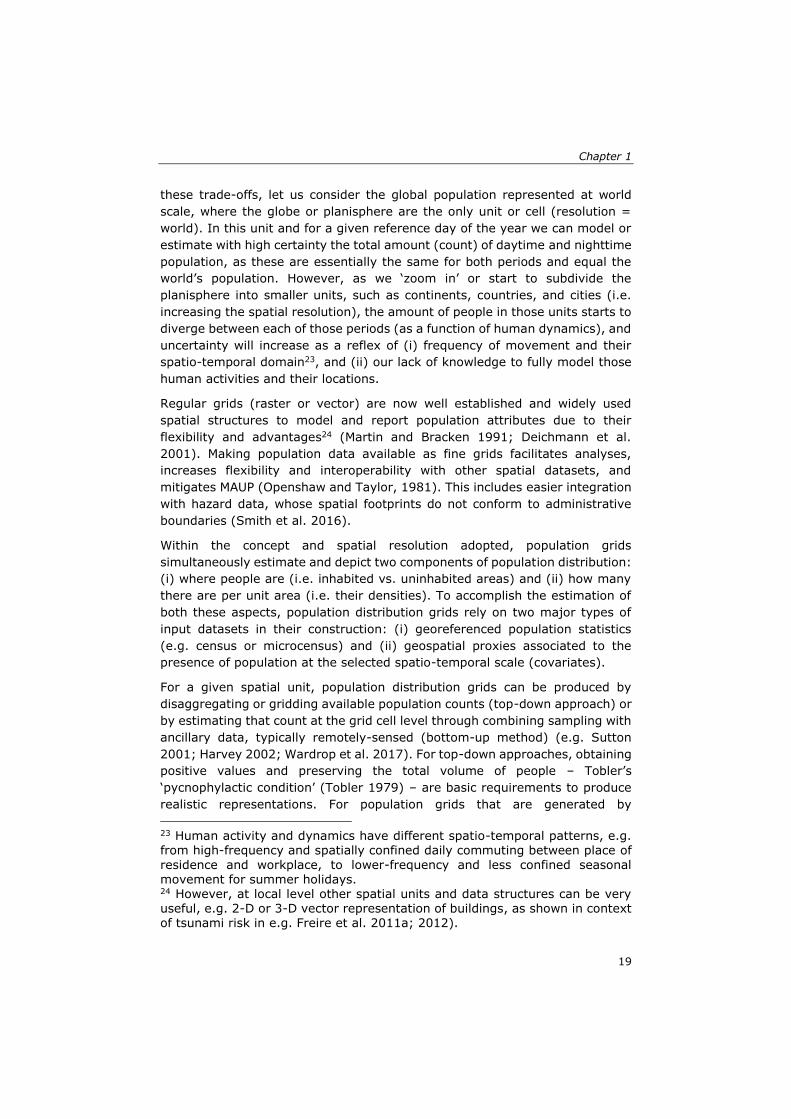
Chapter 1
19
these trade-offs, let us consider the global population represented at world
scale, where the globe or planisphere are the only unit or cell (resolution =
world). In this unit and for a given reference day of the year we can model or
estimate with high certainty the total amount (count) of daytime and nighttime
population, as these are essentially the same for both periods and equal the
world’s population. However, as we ‘zoom in’ or start to subdivide the
planisphere into smaller units, such as continents, countries, and cities (i.e.
increasing the spatial resolution), the amount of people in those units starts to
diverge between each of those periods (as a function of human dynamics), and
uncertainty will increase as a reflex of (i) frequency of movement and their
spatio-temporal domain23, and (ii) our lack of knowledge to fully model those
human activities and their locations.
Regular grids (raster or vector) are now well established and widely used
spatial structures to model and report population attributes due to their
flexibility and advantages24 (Martin and Bracken 1991; Deichmann et al.
2001). Making population data available as fine grids facilitates analyses,
increases flexibility and interoperability with other spatial datasets, and
mitigates MAUP (Openshaw and Taylor, 1981). This includes easier integration
with hazard data, whose spatial footprints do not conform to administrative
boundaries (Smith et al. 2016).
Within the concept and spatial resolution adopted, population grids
simultaneously estimate and depict two components of population distribution:
(i) where people are (i.e. inhabited vs. uninhabited areas) and (ii) how many
there are per unit area (i.e. their densities). To accomplish the estimation of
both these aspects, population distribution grids rely on two major types of
input datasets in their construction: (i) georeferenced population statistics
(e.g. census or microcensus) and (ii) geospatial proxies associated to the
presence of population at the selected spatio-temporal scale (covariates).
For a given spatial unit, population distribution grids can be produced by
disaggregating or gridding available population counts (top-down approach) or
by estimating that count at the grid cell level through combining sampling with
ancillary data, typically remotely-sensed (bottom-up method) (e.g. Sutton
2001; Harvey 2002; Wardrop et al. 2017). For top-down approaches, obtaining
positive values and preserving the total volume of people – Tobler’s
‘pycnophylactic condition’ (Tobler 1979) – are basic requirements to produce
realistic representations. For population grids that are generated by
23 Human activity and dynamics have different spatio-temporal patterns, e.g. from high-frequency and spatially confined daily commuting between place of
residence and workplace, to lower-frequency and less confined seasonal movement for summer holidays. 24 However, at local level other spatial units and data structures can be very useful, e.g. 2-D or 3-D vector representation of buildings, as shown in context of tsunami risk in e.g. Freire et al. 2011a; 2012).

Introduction, Context and Objectives
20
disaggregating available statistics (top-down) while preserving their volume,
output accuracy (with respect to ground truth data) is largely dependent on
the spatial detail and quality of input geospatial layers (Freire et al. 2018a).
In the spatial refinement of existing population statistics (top-down), many
approaches have been tested and used (Wu et al. 2005), but most are
variations of the classical dasymetric mapping technique (Semenov-Tian-
Shansky 1928; Wright 1936). Dasymetric mapping is a simple yet powerful
cartographic technique that allows limiting the distribution of a variable to the
zones where it is present by using related ancillary information in the process
of areal interpolation (Eicher and Brewer 2001). The technique has been
progressively revived and refined in last two decades, namely with
development of ‘intelligent dasymetric mapping’ variants (Mennis 2003;
Mennis and Hultgren, 2006).
In dasymetric mapping of population, the quality of the proxy variable(s) is
more important than the choice of the downscaling method/algorithm (Martin
et al. 2000). Hence, all other factors being equal, the factors determining the
output accuracy of the final map (grid) can be ranked as follows:
1. Detail (resolution) and quality of source zoning population (i.e. census
statistics),
2. Quality of proxy variable (covariate) for population disaggregation,
3. Specific methodology applied for disaggregation from source zones to
target zones.
Then for disaggregating global population grids based on dasymetric mapping
(either using one or more covariates as input), the challenge can be narrowed
to two aspects: (i) obtaining reliable geospatial population statistics, and (ii)
creating an appropriate proxy (target) layer associated to the presence of
population at the selected spatio-temporal scale (i.e. covariate). In most
population disaggregation approaches, significant effort and cost is expended
preparing, combining and modeling geographic variables in order to obtain an
appropriate proxy layer or probability surface to support population
disaggregation (e.g. WorldPop25). In developing more detailed multi-temporal
global population grids, this thesis (Chapter 5) has focused instead on aspects
(1) and (2) mentioned above.
1.2.4.1 Global Population Grids
At global level, starting in the 1990s the increased availability of digital spatial
data combined with improved capabilities of Geographic Information Systems
(GIS) have enabled the development of several global population distribution
grids, such as the GPW (Tobler et al. 1995), HYDE (Goldewijk and Battjes
25 https://www.worldpop.org

Chapter 1
21
1997), LandScan (Dobson et al. 2000), and GRUMP (Balk et al. 2005)26. These
grids vary in regards to population concept, data sources, and modeling
approach – for a detailed review of current large-scale gridded population data
products, see Leyk et al. 2019.
Although global population grids have been available for more than two
decades, constraints have limited their usability for some applications (Hay et
al. 2005; Linard and Tatem 2012; Mondal and Tatem 2012). Among these are
their coarse spatial resolution (maximum was 30’’), use of dichotomous maps
of built-up in their construction, and coarse, limited, and incomplete
discrimination of urban areas and settlements (especially smaller ones) (Potere
and Schneider 2007; Potere et al. 2009). Better and finer global analyses of
population-environment interactions require enhanced geoinformation on
population distribution and densities, in particular concerning temporal and
spatial resolution and capacity for change assessment. For global change
detection and assessment, having a clear and coherent spatio-temporal
production model is important to ensure users’ confidence and allow
comparisons in space and time (Freire et al. 2016a). Because even if conducted
at global scale, exposure assessment to some hazards is highly sensitive to
spatial resolution of population grids: e.g. tsunamis, river floods, landslides.
In the modeling of population distribution, geo-information science and Earth
observation play an increasingly important role (Leyk et al 2019). These
technologies have been contributing in several ways to improving population
modeling for decades (Tenerelli et al. 2015), but more recent developments in
imagery and methods for information extraction have been evolving towards
constituting a more detailed, objective and independent data source on human
presence on the Earth surface. The combination of new cost-effective,
automated and fully replicable data classification methods (e.g. machine
learning) with the synoptic capacities of satellite Earth Observation imagery,
made accessible in a public, full open-and-free frame, can contribute to fill
information gaps. This is especially true in poor, remote, unsafe, disputed, very
large, and/or highly dynamic areas of the globe where conventional data
gathering and updating is challenging (Freire et al. 2018a).
At global level, these developments have enabled global mapping of built-up
areas and settlements with unprecedented spatio-temporal detail, consistency,
and temporal coverage – in essence capturing the local scale with global
coverage. These new remotely-sensed global datasets include the Global
Human Settlement Layer (GHSL) (Pesaresi and Ehrlich 2009; Corbane et al.
2017), mining both optical and radar imagery in the period 1975-2016, and
26 These were the only global gridded population data products available when work for this thesis was initiated.
Introduction, Context and Objectives
22
the Global Urban Footprint (GUF) for 2012, generated from radar satellite
constellation of TerraSAR-X and TanDEM-X (Esch et al., 2017).
Making these datasets available open and free, as in the case of GHSL, helps
to increase access, promotes transparency, and ensures accountability of the
information produced. GHSL’s enhanced spatio-temporal mapping of buildings
and density of built-up areas offers a suitable proxy for the location of people
and, as such, is being used for enhancing multitemporal global population
grids, such as GHS-POP (covering the period 1975-2015) and WorldPop
(covering years 2000-2020), and to create time series of population estimates
that can be used to fill in data gaps between national census surveys that are
commonly taken at decadal intervals (Nieves et al. 2018). In the case of
WorldPop, built-up areas are being used in combination with other spatial
covariates to create population grids (Stevens et al. 2015).
Box 1.1 The GHS-POP gridded population time series The Global Human Settlement Population Grid (GHS-POP) depicts the distribution and density of the total population as the number of people per
grid cell (at 250 m spatial resolution) for nominal epochs 1975-1990-2000-2015. Using dasymetric mapping, residential population estimates (counts) per smallest census unit available, provided by CIESIN GPWv4 for the years of interest, are disaggregated to grid cells informed by the distribution and density of built-up areas as mapped by GHSL (GHS-BUILT) for matching epochs (Freire et al. 2016a; 2018). At time of first public release (2016) GHS-POP was the highest resolution
gridded global population time series and remains the only detailed such dataset spanning the last 40 years. Respect to previous global time series, GHS-POP innovated by increasing spatial resolution by a factor of 16 (from
~1 km to 250 m) while improving temporal depth respect to other global gridded series (GPW, GRUMP), and by representing both population counts and densities by using an equal-area projection (World Mollweide). It is the only disaggregated global dataset relying on a single, time-specific, and
consistent proxy (built-up areas), limiting the risk of circularity and endogeneity in analyses. For latest release, areas declared as unpopulated were revised critically and the representation of population along coastlines was improved (Freire et al. 2018a). In order to increase their usability (Lewis 2014), since 2019 these grids are also provided in two different coordinate systems (addition of WGS84), and can be downloaded as bulk or in regular
tiles. Global mapping of built-up areas was performed through the Global Human Settlement Layer (GHSL) project using Landsat imagery collections for nominal epochs 1975, 1990, 2000 and 2014 (Pesaresi et al. 2013; 2016). The GHSL approach is grounded on the concept that buildings and their agglomerations (i.e., settlements) are nowadays the main visible and direct manifestation of human presence (and activity) on the Earth’s surface.
GHS-POP is part of an integrated suite of geospatial products, aiming to constitute a detailed and consistent time series of lightly modeled population distributions that is based on reproducible methods for sustainable data production (Melchiorri et al. 2019) and can be used in policy support in

Chapter 1
23
numerous domains (Ehrlich et al. 2018a), including monitoring exposure
trends (Ehrlich et al. 2018b). These grids are created using consistent, open and free input data integrated using a clear and transparent approach and are also freely accessible and downloadable at https://ghsl.jrc.ec.europa.eu/ghs_pop2019.php (last access: 30 September 2019).
At continental level, new big earth data analytics are also enabling sustained
mapping of built-up areas at high spatial resolutions, such as the European
Settlement Map (ESM) (Ferri et al. 2014). Detailed mapping of built-up areas
(at 10 m) from ESM was combined with an enhanced LULC map to disaggregate
detailed census 2011 data for producing the most detailed pan-European grid
of resident population (100 m) spanning 43 countries (Freire and Halkia 2014).
For several countries a model was developed to increase the spatial resolution
of source census data and population was gridded at 10 m, to fully preserve
the maximum resolution of census data. Also, a new disaggregation approach
was developed with two levels, where land use land cover determines
reallocation of population within source zones, and built-up density determines
specific densities at the grid cell level. The latter population grids showed
promise for improving DRM operations at local scale, namely in frame of
Copernicus EMS Mapping27 activities (Freire et al. 2015c). ESM is now in its
third version, with Symbolic Machine Learning (SML) supervised classifier, the
PANTEX and the morphological image features being employed to map
buildings for 39 countries from multi-sensor very high resolution optical
imagery (multispectral and panchromatic) for reference year 2015, totaling
~127TB of data (Sabo et al. 2019). An added-value to the previous versions is
the improved automatic detection of buildings, automatic extraction of water,
extraction of building typology (residential vs. non-residential) and an
information layer allowing to derive city indicators (Corbane and Sabo 2019).
These data are expected to benefit modeling of population distribution.
Other developments in population and settlement mapping are progressing on
a country basis, such as the High Resolution Settlement Layer (HRSL) (Tieke
et al. 2019). CIESIN is producing and providing population distribution grids at
a resolution of 1 arc-second (~30 m) for 2015, based on settlement extents
extracted from very high-resolution (0.5 m) satellite imagery by the
Connectivity Lab at Facebook, using convolutional neural networks (CNN).
1.2.4.2 Increasing temporal resolution and integrating unconventional data sources
Census figures register where people reside and usually sleep28, although their
spatial distribution varies widely over daily, seasonal and long term time scales
27 https://emergency.copernicus.eu/mapping/ems/emergency-management-service-mapping 28 Within the definition of ‘usual residence’ for resident population concept; resident population is usually taken as an approximation of nighttime

Introduction, Context and Objectives
24
(Sutton et al. 2003). This variation in both space and time can be seen as the
static and the dynamic components of population distribution. In this view the
static component typically refers to the number of inhabitants per mapping
unit (and their characteristics), whereas the dynamic component results from
their activity patterns, and their distribution along the spatial and temporal
dimensions (van Westen et al. 2013). Due to the diverse locations of human
activities (e.g. work, study, leisure) and the displacements they induce, the
spatial distribution of population is strongly time-dependent, particularly in
metropolitan areas, characterized by intense commuting flows29 (Foley 1952;
1954; Schmitt 1956). However, these high frequency dynamics are often not
captured by available population data sources at needed spatio-temporal
scales, and typically require geospatial modeling for their representation as
spatially-explicit data. Especially for disaster risk management in urban areas,
it is the population variation during the daily cycle that is particularly relevant,
and in this respect the most important determination is whether an incident
occurs at night or during the day (Dobson 2007; Alçada-Almeida 2009).
Incidentally, a number of prominent contemporary disasters occurred during
the daytime period, e.g.: 9/11 attacks (USA, 2001) between 8:46 – 10:28 am;
2010 Haiti Earthquake, at 4:53 pm; 2011 Great Tohoku Earthquake and
Tsunami, at 2:46 pm (all local times). These events occurred when a large
share of the population was in workplaces, schools, etc. This implied that even
detailed, accurate and current population distribution maps based on census
data (i.e. resident population), if available, were rendered mostly operationally
useless for Emergency Management (Response).
Modeling population distribution at high temporal resolution (e.g. day vs.
night) is especially challenging regarding the two main tasks or steps involved,
i.e. (i) obtaining or estimating stocks of population groups for given zones and
time periods, and (ii) disaggregating or allocating these population counts to
respective target units or place of activity (Martin et al. 2015). For very
localized areas of interest (AOI) and limited temporal events (e.g. a stadium
during a football match) this is relatively straightforward, as the problem is
limited to mapping the expected population (i.e. attendance volume) present
at the event in the area of the event. However, it becomes increasingly
challenging as the study area increases, given the need to balance the
population budget and correctly subtract the attendance from the surrounding
areas it originated from and where it is not present during the event (e.g. using
an origin-destination matrix). To further complicate matters, daytime
population, in what is clearly a simplification of a more complex reality of population distribution during that period. 29 It should be noted that also residential population is subject to dynamics and displacement, and that these can be especially quick and intense in case of conflict or other crises (e.g. in Syria, see Corbane et al. 2016).

Chapter 1
25
population distribution can be considerably different in a working or a weekend
day or holiday.
Twenty years ago, the LandScan project (Dobson et al. 2000) has incorporated
the temporal dimension in global population distribution by mapping ‘ambient’
population30, an “average population distribution over a 24-hour period”
(Badhuri et al. 2002) that “integrates diurnal movements and collective travel
habits into a single measure” (Dobson et al. 2000). Conceptually, by straying
away from residence-based population density, this representation may be
more adequate for assessing exposure for daytime hazard events or those
having slow onset, affecting populations over a wide temporal window (e.g.
pollution, epidemics, toxic release). The latter case is especially fitting owing
to the low temporal specificity of LandScan Global data. However, LandScan’s
spatial resolution (30 arc-seconds, ~1 km at Equator), while acceptable for
most global and national analyses, is insufficient for most sub-national
requirements. Furthermore, ambient population corresponds to a compromise
between daytime and nighttime distributions that strictly represents neither
period.
Meeting the need for more temporally-explicit representations, two subsequent
population distribution databases having higher temporal and spatial detail
were developed for the territory of the USA: a team at Los Alamos National
Laboratory mapped day- vs nighttime and indoor and outdoor populations at
250 m (McPherson and Brown 2004; McPherson et al. 2004), and LandScan
USA started modeling day- vs night populations (Bhaduri et al. 2002), then
evolving into mapping their distributions also on weekends and special events
(Bhaduri et al. 2007). Outside of the US, a few ad-hoc efforts succeeded in
providing such important improvements, most at local level and even fewer at
national scale: these include models for Helsinki (Ahola et al. 2007), the UK
Population 24/7 project (Martin et al. 2010), work for Lisbon (Freire 2010;
Freire et al. 2012; 2013), the DynaPop model (Aubrecht et al. 2014), and a
series of models for Tokyo (Osaragi 2009; 2016). Such models typically rely
on intensive geospatial and/or statistical databases on time usage, which are
usually only available for selected areas and often at a high cost. This raises
the issue of the sustainability of approaches, an important requirement for
continued support to DRM activities. Building on the high resolution European
Settlement Map (ESM) built-up layer (Ferri et al. 2014), Freire et al. (2015b)
have proposed an approach based on available free data (the ‘NDPop’ model)
enabling the refinement of the spatial distribution of resident population and
the addition of a temporal dimension to population data (day- vs night),
wherever a LULC map is available (e.g. whole Europe). However, in this model
30 Despite this distinct definition, the concept is commonly abused in scientific literature as representing ‘residential’ population.

Introduction, Context and Objectives
26
the discrimination of daytime population is dependent on the quality of
LandScan global grid of ambient population.
In recent years, a number of emerging data sources and technologies were
explored for direct mapping of population or as alternative proxies for its
disaggregation, but mainly as proof-of-concept. These include mobile phones
(Deville et al. 2014), crowdsourcing/Volunteered Geographic Information
(VGI) (Bakillah et al. 2014), and location-based social media (LBSM) (Aubrecht
et al. 2011; 2017). LBSM appears especially valuable for dynamic population
distributing modeling by providing information both on time usage and on
target zone characterization (Aubrecht et al. 2017a). However promising, a
number of issues involve these types of data and technologies, e.g.
sustainability of approaches, data access and ownership, privacy and
anonymity of social media users, and representation bias (Zhang and Zhu
2018). The main challenge for developers and users is how to scale up highly
localized approaches to wide geographical areas (continents, world) and
provide datasets open and free.
Considering the trade-offs mentioned above, mapping the dynamics of
population is especially challenging for large, multi-national areas and typically
involves intensive work of identifying, mining, combining and matching
heterogeneous statistical and spatial data from disparate sources. This requires
significant investment in data integration and harmonization, to improve and
supplement limitations of single remote sensing and conventional map sources
(Lloyd et al. 2019). The combination of conventional (remote sensing data,
LULC maps) with unconventional big geospatial data sources (VGI, POIs) is
allowing overcoming some of the previous challenges and gaps, such as
improving accuracies, increasing temporal resolution, while covering wide
geographical areas (Ye et al. 2019; Yang et al. 2019). The project ENACT31
(ENhancing ACTivity and population mapping) succeeded in producing the first
continent-wide (28 countries of EU), consistent, seamless, high-resolution and
validated population density grids that take into account both daily and
seasonal variations: day- and nighttime grids per month of the year were
produced at 1 km resolution32, for 2011 (Batista e Silva et al. 2018), accounting
for workers, students, and visitors. This effort was aided by technical advances
and increased availability and access to various big data sources that enabled
the detailed mapping of land use and activities (Rosina et al. 2018). In the
context of risk analysis and DRM, we have combined the ENACT population
31 https://ghsl.jrc.ec.europa.eu/enact.php 32 Although in ENACT it was possible to decrease the trade-off between
geographical coverage and temporal resolution, there remains the typical trade-off between spatial and temporal resolution: although the latter resolution has increased 24-fold, this was only possible at 1 km spatial resolution, or 100 times lower detail than previous best-available Pan-European resident population grids (100 m), by Freire and Halkia (2014).

Chapter 1
27
grids with the most recent pan-European hazard data on flood and seismic
hazard, in order to map and quantify variations of population exposure, to
study their spatio-temporal patterns, and to identify potential daily and
seasonal exposure hot spots (Freire et al. 2018b; Schiavina et al. 2018).
In brief, for effective support to DRM, geospatial population data should be
accurate, trusted and reliable (UNDRR 2019). Furthermore, it should be up-to-
date, have sufficient resolution (spatial, temporal, thematic), and be readily
available (i.e. produced beforehand or rapidly computable on-demand)
through sustainable and reproducible methods. Such population data are still
lacking for many countries and regions, both rich and poor, and conducting
DRM at global scale would benefit from complete, consistent, and integrated
datasets.
1.3 Objectives and structure of the Dissertation The mapping of human distribution and population exposure has generally
lagged behind hazard modeling and mapping, in terms of accuracy, detail, and
currency. The main objective of this research was to develop methods to
improve the mapping of population distribution across multiple spatio-temporal
scales in support of Disaster Risk Management. This thesis comprises
contributions of population distribution modeling to advancing Disaster Risk
Management and Reduction efforts by:
(i) developing several geospatial models that improve (in detail,
currency, quality) representation/mapping of population distribution at
a range of spatial and temporal scales (Chapters 2, 3, 5),
(ii) applying those data to real disaster risk scenarios for different
hazard types by combining geospatial population layers with hazard
maps (Chapters 2, 3, 4, 6),
(iii) using spatial analysis for assessing human exposure, including
quantitative and qualitative analyses, map representations and
visualization (Chapters 2, 3, 4, 6).
We progress from local to global coverage, following specific modeling capacity
and requirements at local level with increasing ability to bring improvements
to the global domain. The research supporting this work, still ongoing, has
taken place over a period of 9 years (concurrent with other research activities
and topics) and has so far comprised more than 50 scientific and technical
publications. The five core chapters are published as peer-reviewed
publications, four of them as articles in different ISI-indexed journals.
With each model development and application, we aim to contribute to
answering a set of questions, as presented in Error! Reference source not f
ound.. This table also shows the overall objectives and the range of different
issues addressed in each chapter.

Introduction, Context and Objectives
28
Table 2 Overview of Chapters in this Thesis
Chapters Objectives Key Questions Issues Addressed
2. Modeling of spatio-temporal distribution of urban population at high-resolution – value for risk assessment and emergency management
To demonstrate and discuss the value for risk assessment and emergency management of modeling the distribution of urban population at higher spatial and temporal resolutions, to enable local-level analyses.
Is the spatial distribution of urban population in the daily cycle relevant for risk analysis (exposure) at local scale?
How can more detailed modeling of spatio-temporal distribution of urban population contribute to DRM, considering its cycle?
Relevance of spatially-explicit population data for DRM/emergency management.
Approaches to map population distribution in space and time.
Uses and benefits of detailed day and nighttime population distribution grids are illustrated for four different disaster scenarios, natural and man-
made.
Spatio-temporal characteristics of disaster development for population exposure.
3. Integrating population dynamics into mapping human exposure to seismic hazard
To improve earthquake risk analysis at regional level (metropolitan area) to benefit decision support for disaster and emergency management by (i) modeling and mapping nighttime and daytime population distribution at high spatial resolution, (ii) investigating spatio-temporal population exposure to earthquake hazard and (iii) classifying exposure levels through the combination of
Can new geospatial data on spatio-temporal distribution of population, derived by scaling-up a costly local-based approach, be combined with an earthquake hazard map to improve human exposure mapping and assessment in a metropolitan area?
What is the estimated variation in population exposure by seismic level in the Lisbon Metropolitan Area
Importance of population dynamics for disaster risk assessment.
GISc research needs in DRM.
Development and testing a high resolution data-based model to map the nighttime and daytime population distributions at metropolitan level, by scaling up a local-level model.
Mapping and assessing human exposure to different seismic hazard levels in

Chapter 1
29
Chapters Objectives Key Questions Issues Addressed
population densities with seismic hazard levels to derive and propose new fine-scale composite human exposure maps.
To improve modeling and mapping of population distribution for enhanced assessment of population exposure to hazards at regional level (metropolitan area).
(LMA) in day- and nighttime periods?
day- vs nighttime periods, demonstrated with real seismic scenario in Lisbon Metropolitan Area (Portugal).
Visualization and communication of human exposure.
Potential implications of results for DRM.
4. Advancing tsunami risk assessment by improving spatio-temporal population exposure and evacuation modeling
To improve the assessment of tsunami risk and contributing to more efficient and effective DRM by considering the time dependence (daily cycle) of population exposure and
evacuation from this hazard in a metropolitan area.
How is the spatio-temporal distribution of population in the daily cycle in a metropolitan area relevant for population exposure to and evacuation from tsunami hazard?
Tsunami hazard, population exposure, and risk.
Modeling and mapping evacuation time in day and nighttime periods.
Potential implications of results for DRM.
5. Enhanced data and methods for improving open and free global population grids: putting ‘leaving no one behind’ into practice
To test data and methods to mitigate deficiencies affecting global collections of census data, for improving open and free global population distribution grids.
How can some major shortcomings in geospatial population statistics be detected, assessed, and mitigated with remote sensing information and automated approaches, while preserving the statistic’s integrity for policy making?
Characteristics and requirements of population data and grids for international policy support.
Taxonomy of shortcomings affecting geospatial population statistics.
Potential sources of detected anomalies

Introduction, Context and Objectives
30
Chapters Objectives Key Questions Issues Addressed
and inconsistencies.
Shortcomings present in global collections of census data, by introducing, applying, and discussing novel procedures aimed at investigating and detecting some of those major anomalies.
Automated detection of some detected inconsistencies using high resolution geospatial data derived from remote sensing.
Automated mitigation of inconsistencies using the ‘split and merge’ approach.
6. An Improved Global Analysis of Population Distribution in
Proximity to Active Volcanoes, 1975–2015
To characterize with unprecedented detail the spatio-
temporal changes in the distribution of human population in proximity to historically active volcanoes by combining detailed geospatial grids of global population densities for the 1975–1990–2000–2015 periods with the latest data on distribution of volcanoes on Earth, considering both Holocene volcanoes and those having
How has resident population distribution and density been
varying at global and regional scales (South East Asia, and Central America) in proximity to historically active volcanoes in period 1975-2015, and what is the current situation?
To what extent does a new model and data on spatio-temporal distribution of population (decadal cycle) improve global and
Volcanic hazards, population exposure, and risk.
Data requirements
for assessing population exposure and how to narrow gaps.
Contribution of GHSL to DRM.
Technical challenge of measuring accurately both distances and areas in global maps.
Variation of population distributions with distance to Holocene

Chapter 1
31
Chapters Objectives Key Questions Issues Addressed
significant eruptions.
To conduct more updated and refined global and regional assessments of population distribution in proximity to historically active volcanoes based on new and improved multi-temporal (long cycle, inter-annual) global population grids, and investigate and estimate globally the recent evolution (over 40 years) and current distribution of population in relation to historic volcanism.
regional characterization of population living in proximity to volcanoes and the assessment of population potentially affected by their hazards?
volcanoes and those with significant eruptions, 1975-2015.
Potential implications for DRM.
To summarize the chapter contents, Chapter 2 sets the stage for the thesis
by demonstrating and discussing the value for risk analysis and emergency
management of modeling the distribution of urban population at higher spatial
and temporal resolutions, to enable local-level analysis. Uses and benefits of
detailed day- and nighttime population distribution grids are illustrated for four
different disaster scenarios (using fictitious hazard data), either natural and
man-made, at municipal level.
Chapter 3 departs from the population distribution model from Chapter 2 and
scales it up to regional level (the Lisbon Metropolitan Area) to improve
modeling and mapping of population distribution for enhanced assessment of
population exposure to earthquake hazard, which is quite relevant in the study
area. The chapter discusses how to benefit decision support for disaster and
emergency management by (i) modeling and mapping nighttime and daytime
population distribution at high spatial resolution, (ii) investigating spatio-
temporal population exposure to earthquake hazard and (iii) classifying
exposure levels through the combination of population densities with seismic
hazard levels to derive and propose new fine-scale composite human exposure
maps. This constitutes the first known integration of explicit and detailed

Introduction, Context and Objectives
32
spatio-temporal population dynamics into mapping human exposure to seismic
hazard in a metropolitan area.
In Chapter 4 we address improvements to the assessment of tsunami risk and
contributions to more efficient and effective DRM by considering the time
dependence (in the daily cycle) of population distribution in a metropolitan
area, where this hazard is rather significant. In addition to assessing variation
of human exposure, we conduct a simulation of evacuation from this hazard in
day- and nighttime periods. This work provides a pioneering example of the
integration of spatio-temporal population dynamics to assess exposure to
tsunami for a whole metropolitan area.
Chapter 5 is more policy focused, concerned with characteristics and
requirements of population data and grids for supporting requirements of post-
2015 international development agreements (e.g. SDGs, Sendai) and
respective indicators. In this chapter we develop /explore/propose new
automated approaches to detecting, assessing, and mitigating some of the
major deficiencies present in global geospatial population statistics using
remotely sensed data and geospatial modeling.
Finally, in Chapter 6 we use the multi-temporal global population grids
enhanced with developments from Chapter 5 to conduct more updated and
refined global and regional assessments of population potentially affected by
volcanism. Based on these improved multi-temporal (long cycle, inter-annual)
population grids, we investigate and estimate globally the recent evolution
(1975-2015) and current distribution of population in relation to historic
volcanism.
In a concluding chapter (Chapter 7) we summarize the main contributions of
the approaches presented in previous chapters, in relation to respective
research objectives and questions, and discuss ongoing and future
developments in modeling population distribution to support Disaster Risk
Management and Reduction.
All chapters (articles) develop and apply new methodologies to solve problems
related to modeling and mapping population distribution and exposure to
hazards, aiming to improve assessment of potential human exposure in their
respective study areas and fields of application (i.e. earthquake, tsunami,
volcanism). Regarding population distribution modeling for DRM, this thesis is
concerned with the total number of people present in a given area. This focus
has the following reasons:
a) For many hazard events, especially sudden ones or those above certain
magnitude, all human beings are approximately equally vulnerable
(Villagrán 2006);

Chapter 1
33
b) Worldwide and in specific regions, the total population count of a
geographical area is still affected by issues and significant uncertainties
(see Chapter 5), therefore benefiting from improvements;
c) If the most simple, basic, and neutral demographic variable (total
population) is still affected by significant uncertainties, it is likely these
are even greater for more complex and sensitive variables (e.g. sex,
age, ethnicity) ;
d) Other attributes of population (e.g. sex, age) are often only available
at coarser scales (i.e. higher administrative levels) than total
population33, and disaggregation and gridding of these variables is
typically conducted applying the ratio from source zones to all
disaggregated total population cells in each zone – therefore
propagating the errors in mapping total population. In this scenario,
improving grids of total population will also benefit mapping of related
demographic attributes.
Each chapter puts these developments in their respective context, justifies why
new data is needed and demonstrate its usability and contribution to analysis
of human exposure and DRM. In addition, Chapters 2, 3, 4, and 6 show
development of improved population distribution grids and their application to
specific hazard scenarios, natural and man-made. These population grids were
produced using variations of the ‘dasymetric mapping’ approach, and these
layers were previous unavailable for the respective study areas at these spatio-
temporal resolutions.
With the exception of Chapter 2, which uses fictitious hazard data, all analyses
assess population exposure by relying on best-available hazard maps and data
for the respective study areas. Table 3 summarizes the main characteristics of
chapters in this thesis in relation to main research topics and concepts.
33 As confirmed in CIESIN GPWv4.11 metadata: https://sedac.ciesin.columbia.edu/downloads/docs/gpw-v4/gpw-v4-documentation-rev11.pdf

Introduction, Context and Objectives
34
Table 3 Main characteristics of chapters in this thesis in relation to main research topics and concepts; main innovative aspects highlighted in bold

Chapter 1
35
Table 4 (cont.) Main characteristics of chapters in this thesis in relation to main research topics and concepts; main innovative aspects highlighted in bold

Introduction, Context and Objectives
36

37
Chapter 2. Modeling of spatio-temporal
distribution of urban population at
high-resolution – value for risk
assessment and emergency
management34
34 This chapter is published as:
Freire, S., 2010. Modeling of spatio-temporal distribution of urban population at high-resolution – value for risk assessment and emergency management. In: Konecny, M., Zlatanova, S., Bandrova, T.L. (eds.), Geographic Information and Cartography for Risk and Crisis Management. Lecture Notes in Geoinformation and Cartography. Springer Berlin Heidelberg, pp. 53-67.

Modeling of spatio-temporal distribution of urban population at high-resolution – value
for risk assessment and emergency management
38
Abstract Knowing the spatiotemporal distribution of population at the local scale is
fundamental for many applications, particularly in risk analysis and emergency
management. Because of human activities, population counts and their
distribution vary widely from nighttime to daytime, especially in metropolitan
areas, and may be misrepresented by census data. This study uses a
dasymetric mapping approach to refine population distribution in Portugal. The
most recent census enumeration figures and mobility statistics are combined
with physiographic data to allocate nighttime population to residential areas,
and workplaces and workforce are georeferenced to model daytime
distribution. Main results represent expected maximum daytime population
and maximum nighttime residential population for each 25-m grid cell in the
study area. Since the same spatial reference base is used to allocate
population, day and night distributions are directly comparable, as is
demonstrated in sample applications in the context of emergency
management. Verification and validation procedures and demonstrations
indicate that the approach suits the objectives.
2.1 Introduction
2.1.1 Population distribution and emergency management
Natural or man-made disasters, either resulting from natural hazards,
technological accidents, or terrorism, usually occur without warning and can
potentially affect people from a local to a continental scale. Risk is usually
defined as a function of hazard probability and vulnerability, the latter resulting
from a combination of exposure and ability to cope (UNDP 2004).
Misestimating one of these components necessarily affects the accuracy of the
overall risk assessment and mapping.
Human life is unquestionably the most important asset to protect, and the dis-
tribution and density of the overall population is a rather basic geographical
indicator. Therefore accurately estimating population exposure is recognized
as a key component of catastrophe loss modeling, one element of effective risk
analysis and emergency management (FEMA 2004, Chen et al. 2004, NRC
2007). However, until recently, assessment and mapping of human
vulnerability has been lagging behind hazard analysis efforts (Pelling 2004),
and potential loss derived from exposure has served as a quantitative proxy
for risk (Lerner-Lam 2007). Also, updated and detailed mapping of population
distribution is important for decision support in practically every phase of the
emergency management cycle, if produced at appropriate spatial and temporal
scales (Sutton et al. 2003), e.g., central to the planning stage is the
assessment of population exposure and vulnerability in the hazard zone;
mitigation includes reducing vulnerability and exposure (namely by displacing
population or other measures); preparedness may involve fitting and placing

Chapter 2
39
means and resources according to vulnerability, for more efficient response in
case of disaster; during and after the event, locating and estimating victims is
essential to tailor response and rescue efforts, including allocating emergency
personnel, hospital beds, etc.; and finally, estimating all activities and people
affected, even if indirectly, facilitates the recovery process.
Despite recent efforts by Dobson (Dobson 2003, 2007) at devising a population
estimation technique that could be employed in real time once a disaster
occurs, for planning and simulation purposes and to ensure a timely response,
adequate population distribution data should be produced and made available
beforehand whenever possible.
2.1.2 Population in space and time
The increased availability of digital spatial data combined with improved
capabilities of Geographic Information Systems (GIS) have allowed for the
development of several global population distribution databases, such as the
GPW, HYDE, and LandScan (Tobler et al. 1995; Goldewijk and Battjes 1997;
Dobson et al. 2000). However, their spatial resolution is still too coarse to
adequately support analysis at the local level and most do not represent the
dynamics of population distributions. Dobson acknowledges that “even finer
resolutions are needed for many types of disasters”, namely those that can
“impact areas as small as a neighborhood, city block, or single building”
(Dobson 2002). Data sets may be produced globally, but people are always
affected locally.
Due in part to the complex nature of population as a geographical variable,
several approaches have been adopted to estimate their spatial distribution,
including statistical modeling (correlation), surface modeling, and cartographic
methods (Fisher and Langford 1996; Wu et al. 2005). However, many of these
methods require assumptions that over-simplify the reality or disaggregate
population totals based on heuristic or empirical parameters. Additionally,
obtaining positive values and preserving the total volume of people—Tobler’s
“pycnophylactic condition” (Tobler 1979)—are basic requirements to produce
realistic representations. Dasymetric mapping is a cartographic technique,
originally used for population mapping, which aims at limiting the distribution
of a variable to the areas where it is present, by using related ancillary
information in the process of areal interpolation (Eicher and Brewer 2001).
Population distributions are not static in time, varying over daily, seasonal, and
long term time scales (Sutton et al. 2003) due to a number of human activities,
such as work and leisure. For emergency planning in urban areas, it is the
population variation during the daily cycle that is particularly important to be
able to estimate the number, age, and socioeconomic classes affected by an
impact (Alçada-Almeida 2009). In Portugal, as in most countries, existing
population distribution maps and vulnerability or exposure analyses are

Modeling of spatio-temporal distribution of urban population at high-resolution – value
for risk assessment and emergency management
40
normally based on census data, often aggregated at the commune level (e.g.,
Oliveira et al. 2005). Census figures register where people reside and usually
sleep, although their spatial distribution varies widely between night and day,
especially within metropolitan areas. Due to daily commuting alone, the
daytime population of municipalities in the metro areas of Lisbon and Porto can
differ by more than 50% of the official census figures (INE 2003). Also, the
availability of a total count for census or administrative areas creates problems
for analysis (e.g., MAUP, ecological fallacy), being generally assumed that the
distribution is constant and exhaustive in those areas, or represented by their
centroid.
Making population distribution data available as a high-resolution raster data-
base facilitates rapid GIS analysis at the local level and for any zoning.
Therefore, when disaster strikes or is imminent, knowing how many people are
likely to be in the affected area can be invaluable information for adequate
emergency response and evacuation planning. The LandScan project (Dobson
et al. 2000) successfully incorporated the temporal dimension in population
distribution by mapping “ambient population”, a temporally averaged measure
of population density that accounts for human activities (such as sleep, work,
study, transportation, etc.). This representation may be more adequate for
certain applications (such as emergency management) than residence-based
population density. However, LandScan’s spatial resolution (30 arc-seconds),
while adequate for national to global analyses, is insufficient for most practical
uses in Portugal. Furthermore, ambient population corresponds to a
compromise between daytime and nighttime distributions that strictly
represents neither period. Therefore, population distribution databases having
higher temporal and spatial detail are being developed for the territory of the
USA (McPherson and Brown 2004, Bhaduri et al. 2002).
This study is aimed at developing and testing a data-based model to map the
nighttime and daytime population distributions in Portugal at high resolution
to enable local-level analysis. This effort correlates with recent
recommendations to improve vulnerability analyses (Cutter 2003, Balk et al.
2006, Birkmann 2007).
2.2 Methods Pre-processing and modeling of geographical data were conducted in ESRI®
ArcGIS 9.1, a GIS application. GIS offers the necessary tools and flexibility to
implement raster or vector-based dasymetric methods, and was used to verify,
correct, and integrate geographic data sets, and for modeling, analysis, and
mapping the results for presentation.
Because some data sets were made available on a municipal basis, each mu-
nicipality was modeled separately. For each municipality, 25-m raster grids
were created representing different types of population distribution. The raster

Chapter 2
41
structure provides uniform and flexible units that facilitate the reaggregation
for any zoning, thus being suitable for modeling and analysis. A spatial
resolution of 25 m was adopted to approximate the size of a single-family
residence (half block). Also, when the model was tested for sensitivity to cell
size, an increase in resolution to 12.5 m yielded marginal gains in the accuracy
of results.
2.2.1 Study area
The official administrative limits of the municipalities (concelhos) of Cascais
and Oeiras in 2001 constitute the study area for this research. These are two
of the 18 municipalities that comprise the Lisbon Metropolitan Area (LMA), the
main metropolitan area in Portugal (Figure 3).
Cascais and Oeiras occupy 97 and 46 km2, respectively, and have a combined
resident population of 332,811; this results in an average population density
of 2,332 inhabitants/km2, well above the national average density of 112
inhabitants/km2. However, population density varies widely throughout the
study area, from high density in multistory residential apartments to low
density in rural areas. Even at the census block group level, some polygons
are quite large and do not reflect their uneven population density.
This area was selected for several reasons: (a) its characteristics, namely with
regard to urban and suburban character, and strong economic activity, (b) the
availability and access to input data, and (c) personal familiarity with the area,
which facilitates data verification and field work.

Modeling of spatio-temporal distribution of urban population at high-resolution – value
for risk assessment and emergency management
42
Figure 3 Location of the study area in Portugal and in the Lisbon Metro Area (LMA) (Source: CAOP).
2.2.2 Data sets
In this study, the spatial detail of census zones whose counts are to be
disaggregated should be met in scale, resolution, and accuracy by ancillary
data sets used for disaggregation. Input variables used for modeling include
both physiographic and statistical data. In the first group are census tracts,
street centerlines, and land use and land cover (LULC), while the second
includes census counts (INE 2001), data on workforce by workplaces, and
commuting statistics (INE 2003) for the study area. These data were obtained
from various sources and in different formats which are listed in Table 5.

Chapter 2
43
Table 5 Main input datasets used for modeling nighttime and daytime population
Data set Source Date Data type
Street centerlines Private 2004 Vector polyline
LULC (COS90; CLC2000) Public 1990; 2000 Vector polygon
Census block groups Public 2001 Vector polygon
Census statistics Public 2001 Database (MS Access)
Workplaces and employment
Public 2001 Table
Commuting statistics Public 2001 Table (O/D matrix)
In general, temporal consistency among data sets was very high, with the
exception of street centerlines whose reference date was 3 years subsequent
to the model target date (2001). For this reason and owing to the importance
of this data set in the model, it was decided to modify it in order to better
represent the reality of the target date. The LULC data originated from two
maps and was also corrected and improved upon within the study area.
2.2.3 Model
The modeling of population distribution is based on dasymetric mapping using
street centerlines as spatial reference unit to allocate population counts. The
most recent statistical and census data (2001) provide the population counts
for each daily period, while physiographic data sets define the spatial units
(i.e., grid cells) used to disaggregate those counts. This general approach was
successfully implemented by the Los Alamos National Laboratory (New Mexico,
USA) to map daytime and nighttime population distributions in the United
States at 250-m resolution (McPherson and Brown 2004), and is adapted and
applied to Portugal.
An overview of tasks involved in this modeling process is presented in Figure
4. Input data are noted in light gray, secondary products previously unavailable
in Portugal are noted in bold, and main results are noted in bold and darker
gray.

Modeling of spatio-temporal distribution of urban population at high-resolution – value
for risk assessment and emergency management
44
Figure 4 Flowchart of main tasks involved in the model: input data are noted in light gray, secondary products in orange, and main results noted in bold and red
The map of nighttime population distribution was obtained by using a grid bi-
nary dasymetric mapping method to disaggregate residential population from
census zones to residential streets. First, available digital LULC maps were
improved, relevant classes selected, and combined, in order to identify
residential land use. Street centerlines were also modified in order to better
represent the road network existing in 2001. Then, freeways are removed from
consideration and the resulting eligible streets are combined with residential
land use classes from LULC data to obtain residential streets. These are
subsequently rasterized at 25 m and the population from census block groups
(source zones) are interpolated to the respective residential street cells (target
zones) using areal weighting.
The daytime population distribution results from the combination of two com-
ponents (as illustrated in Figure 4): (a) the daytime population in their places
of work or study—the workforce population surface, and (b) the population
that remains home during the day—the daytime residential population grid.
The latter is obtained by multiplying the nighttime distribution by the
percentage of resident population who, according to official statistics (INE
2003), do not commute to work or school. In the absence of other information,
it is assumed that non-commuters remain in their residences in the daytime
period. This implies that this study is not including the potential effects of

Chapter 2
45
leaving home for shopping and several other activities on daytime population
distributions.
The workforce population surface was created by georeferencing 4,316 work-
places and schools and respective workforce and students in the study area;
1,395 of these were georeferenced manually using ancillary data and field
work. The remainder workplaces were geocoded to the street centerlines in
ArcGIS using their addresses. Total daytime population surface results from
the sum of workforce population with daytime residential population on a cell-
by-cell basis. The ambient population distribution is estimated by computing a
weighted average of nighttime and daytime distributions, considering the
proportion of nighttime and daytime periods occurring in a typical 7-day weekly
cycle.
2.3 Results Main results consist of raster surfaces of nighttime (residential) population,
daytime residential population, daytime worker and student population, total
daytime population, and ambient population. These have the number of people
in each 25-m cell in 2001, thus representing population density by 625 m2.
Nighttime and daytime distributions represent maximum expected density on
a typical workday, assuming that everyone is at home at night and all workers
and students are in their workplaces and schools, and the remainder in their
residences. Although still a simplification of reality, it is preferable than
computing a zonal average by census polygon alone.
2.3.1 Verification and validation
Validation of daytime population distribution was limited by unavailability of
compatible reference data sets for Portugal. However, this limitation can be
considered less relevant since daytime population distribution originates from
a combination of the nighttime distribution surface (subject to formal
validation) with mostly official statistical data, as opposed to being derived
from heuristic or empirical weights. Still, the daytime population distribution
was subject to verification in several ways: (a) input data (especially
workplaces’ addresses) were verified through cross-checking with other
sources and field work, regarding location of workplaces (firms), (b) results
were verified with high-resolution imagery to confirm positional accuracy of
distributions, and (c) it was checked that the total number of workers provided
and other statistics (census and mobility) were not contradictory.
The nighttime population distribution was subject to a formal accuracy assess-
ment process, using the higher-resolution census blocks as reference (i.e.,
ground truth) in a correlation analysis. Cell values in modeled distributions
were aggregated by census block in ArcGIS and compared against the
respective census count. Correlation coefficients (Pearson’s r) of 0.84 were

Modeling of spatio-temporal distribution of urban population at high-resolution – value
for risk assessment and emergency management
46
obtained for the municipality of Cascais and 0.79 for the municipality of Oeiras.
Even when the 36 blocks that coincide with block groups are not considered,
the coefficients decrease only slightly to 0.79 and 0.75, respectively. This
indicates that model performance is rather good, in light of its high resolution
and considering the large number of samples used for validation (2,433 census
blocks in Cascais, 1,456 in Oeiras).
2.4 Sample applications Three fictitious case study scenarios are presented as sample applications of
model results in the context of risk analysis and emergency management.
Situations are examples of technological hazards, natural disasters, and
terrorist attack. These scenarios illustrate the usefulness of improved
population distribution mapping for planning or response to actual events.
2.4.1 Case study A: technological hazard (airborne toxic plume release)
A truck transporting highly toxic chemical products is involved in a serious
accident on the off-ramp of a busy freeway in Oeiras, at 11:00 hours (AM). An
airborne toxic plume is released and the dominant winds slowly push it
southwards. Figure 5 represents this scenario, showing the plume and the
daytime population distribution overlaid on orthophotos from 2004.

Chapter 2
47
Figure 5 Case study A: airborne toxic plume release in Oeiras (Source: IGP; TeleAtlas).
2.4.2 Case study B: natural disaster (earthquake)
The Lisbon Metro Area is located in a high seismic risk area, having suffered
destructive earthquakes in the past (e.g., 1755). Around 15:00 hours a strong
earthquake strikes the town of Cascais, causing major damage around
downtown and along the coast. Figure 6 represents this scenario, showing the
area most seriously affected by destruction and collapse of buildings, and the
daytime population distribution overlaid on 2004 orthophotos.

Modeling of spatio-temporal distribution of urban population at high-resolution – value
for risk assessment and emergency management
48
Figure 6 Case study B: earthquake affecting downtown Cascais (Source: IGP; TeleAtlas).
2.4.3 Case study C: terrorist attack (bombing of shopping center)
Around 16:30 hours a powerful explosive is detonated in a large shopping mall
in Cascais, causing great destruction and a fire. Figure 7 represents this
scenario, showing the area most affected by the blast, and the daytime
population distribution overlaid on 2004 orthophotos.
Based on the scenarios presented above, it is relatively straightforward to use
GIS analysis to calculate the affected (exposed) population in each event. Table
6 quantifies and compares exposure based on direct use of census data versus
use of appropriate model results. In all the scenarios there are important
differences in the figures of total exposed population using census data
compared to more appropriate model data. In these daytime scenarios, use of
census data indicates significant under-estimation of affected population, more
dramatic in Scenario C. This could possibly lead the authorities to under-
prepare the emergency response, resulting in an increase of more serious
victims or unnecessary suffering. Also, use of daytime distributions to simulate
and plan for daytime events also improves assessment of exposure and may
contribute to better planning and mitigation measures.

Chapter 2
49
Figure 7 Case study C: terrorist attack in a Cascais shopping center (Source: IGP; TeleAtlas).
Table 6 Total exposed population in each case study
Scenarios Census data
(Block group)
Model results
(Daytime pop.)
Difference
[persons (%)]
A 2,144 3,950 1,806 (84%) B 22,841 28,944 6,113 (26%) C 86 2,151 2,065 (2,400%)
2.4.4 Case study D: planning of best route for hazardous materials transportation
Scenario D illustrates the use of spatiotemporal population distribution in a
planning stage as a criterion for truck routing of hazardous materials between
the A5 freeway exit and a processing facility, in an industrial area of the
municipality of Oeiras. Consideration of population distribution in this context
allows two fundamental issues to be addressed simultaneously: what is the
best period (day or night) and route in order to minimize population exposure
along the way?
In the example, population distribution in a 50-m wide buffer along the streets
is considered as the cost impedance to select the route between two locations
which minimizes overall population exposure. Best routes were computed for
the nighttime period and for the daytime period, considering each period’s

Modeling of spatio-temporal distribution of urban population at high-resolution – value
for risk assessment and emergency management
50
respective population distribution resulting from the model as the sole criterion
(Figure 8).
Figure 8 Case study D: best route considering the population distribution
(Source: IGP; TeleAtlas).
Table 7 quantifies and compares overall population exposure along each route and in each period.
Table 7 Total exposed population along each route and period
Best routes
Exposed population
Length [km]
Nighttime Daytime Difference [persons (%)]
Nighttime 4,9 345 3352 3007 (872%) Daytime 2,7 1001 2734 1733 (173%)
Results show that consideration of spatiotemporal population distribution for
routing leads to definition of quite different routes, having quite different
lengths. Although the best route for the nighttime period is 4.9 km long, only
345 people are within the affected zone, whereas in the daytime period 2,734
people would be exposed along a shorter 2.7-km route. Additionally, total
exposure along the best route for the nighttime period varies widely between
night and day, increasing by 3,007 people to surpass the daytime’s best route
exposure. Therefore, in order to minimize overall population exposure it is the

Chapter 2
51
nighttime period and longest route that should be selected for truck routing of
hazardous materials in the study area.
2.5 Conclusions As the population is not static, it was demonstrated that emergency
management activities would greatly benefit from the use of reliable population
distribution data with increased spatiotemporal resolution for estimation of
human exposure and vulnerability. GIS enables both the development and
spatial analysis’ applications of these data sets. The adopted approach, based
on official data, allows the mapping of nighttime and daytime population
distribution at high spatial resolution, to support local-level analysis. This
method also efficiently accommodates people that work at home, by not
considering that all active population leaves their residences during the
workday. The main value of these results includes the increased spatial resolu-
tion of nighttime distribution, the fact that both nighttime and daytime distribu-
tions share the same spatial reference basis, and that daytime distribution is
better approximated. Furthermore, the combination of both distributions yields
an approximate representation of ambient population. The dasymetric
mapping technique and zonal interpolation meet the requirements for
disaggregation of population counts—obtaining positive values and
preservation of total mass—so the final distribution matches official statistics
and counts.
Given the availability of input data sets, this approach could be applied to all
municipalities (19) comprising the Metropolitan Areas of Lisbon and Porto, that
together contain 40% of Portugal’s population. Subsequent versions would
benefit from a number of improvements: better modeling of “distributed
activities” (e.g., cleaning, security), and accounting for people present in
transportation networks, in hospitals and prisons, or involved in leisure and
shopping activities; increased temporal segmentations of population
distribution, so as to represent differences on a weekly basis (workdays vs.
weekend) or on a seasonal basis (winter vs. summer); and the use of statistical
sources beyond census demographics to consider tourism influx in areas and
periods where that activity is significant. In the context of exposure and risk
analysis, it would also be useful to model people who are indoors versus those
involved in outdoor activities.
Acknowledgement:
The kind support of GeoPoint Lda. throughout this project was greatly
appreciated. The author also thanks the Lisbon Metropolitan Area for providing
data on school facilities, from the Sistema Metropolitano de Informação
Geográfica – Grande Área Metropolitana de Lisboa

Modeling of spatio-temporal distribution of urban population at high-resolution – value
for risk assessment and emergency management
52
53
Chapter 3. Integrating population
dynamics into mapping human
exposure to seismic hazard35
35 This chapter is published as: Freire, S., C. Aubrecht, 2012. Integrating population dynamics into mapping human exposure to seismic hazard. Natural Hazards & Earth Systems Sciences, 12(11):3533-3543.

Integrating population dynamics into mapping human exposure to seismic hazard
54
Abstract Disaster risk is not fully characterized without taking into account vulnerability
and population exposure. Assessment of earthquake risk in urban areas would
benefit from considering the variation of population distribution at more
detailed spatial and temporal scales, and from a more explicit integration of
this improved demographic data with existing seismic hazard maps. In the
present work, “intelligent” dasymetric mapping is used to model population
dynamics at high spatial resolution in order to benefit the analysis of spatio-
temporal exposure to earthquake hazard in a metropolitan area. These night-
and daytime-specific population densities are then classified and combined
with seismic intensity levels to derive new spatially-explicit four-class -
composite maps of human exposure. The presented approach enables a more
thorough assessment of population exposure to earthquake hazard. Results
show that there are significantly more people potentially at risk in the daytime
period, demonstrating the shifting nature of population exposure in the daily
cycle and the need to move beyond conventional residence-based demographic
data sources to improve risk analyses. The proposed fine-scale maps of human
exposure to seismic intensity are mainly aimed at benefiting visualization and
communication of earthquake risk, but can be valuable in all phases of the
disaster management process where knowledge of population densities is
relevant for decision-making.
3.1 Introduction
3.1.1 The importance of population dynamics for disaster risk assessment
Even in the context of natural hazards, risk has several definitions and multiple
approaches exist for its assessment and mapping (Adger, 2006; Birkmann,
2006; Villagran, 2006). The United Nations, for example, define disaster risk
as a function of hazard probability and vulnerability, the latter resulting from
a combination of exposure and ability to cope (UNDP, 2004; UNISDR, 2009).
Among the different types of elements that may be present in hazard zones
(people, property, systems, etc.), human life is unquestionably the most
important value to protect from disasters. The elements of vulnerability and
population exposure are present in some form in all the conceptualizations of
risk and natural disasters, and risk is not fully characterized without an
assessment of those components, in addition to the hazard itself. However,
assessment and mapping of social vulnerability has traditionally been
overlooked in favor of hazard modeling studies (Pelling, 2004; Douglas, 2007).
The development of sophisticated and detailed numerical-based modeling of
hazard zones (e.g. seismic intensity zones, tsunami flood depth, chemical
dispersion models) contrasts with the use of static, generalized, residence-
based representations of population exposure using census data. Nonetheless,
Chapter 3
55
vulnerability is regarded as a greater contributing factor to disaster risk than
the mere existence of hazards (Uitto, 1998; Alexander, 2006; EEA, 2010).
Population exposure refers to the human occupancy of hazard zones (Cutter,
1996), or the population present within the hazard area that would be
potentially directly affected by an event. For many hazard occurrences,
especially those above a certain magnitude or intensity, population exposure
is arguably the greatest determinant of vulnerability and resulting losses and
impacts. Therefore, it has progressively been acknowledged that the accurate
estimation of population exposure as a vital component of catastrophe impact
modeling is an essential element of effective risk analysis and emergency
management (Chen et al., 2004; FEMA, 2004). Despite the study of exposure
and vulnerability to hazards being increasingly at the core of hazards and
disaster research, the inclusion of socioeconomic variables into geospatial risk
models implemented within a Geographic Information System (GIS) remains
a challenge (EC, 2010). Quantifying population exposure as a step for
conducting spatially-explicit risk assessment requires mapping the spatial
distribution of population with sufficient resolution. Population data is therefore
a basic necessity for human exposure analysis, with its quality and level of
detail having a direct effect on response and lives saved (NRC, 2007). Updated
and detailed mapping of population distribution at appropriate spatial and
temporal scales provides an important basis for decision support in every phase
of the emergency management cycle (Sutton et al., 2003; Freire, 2010;
Aubrecht et al., 2012a). Concerning the spatial dimension, disaster risk
reduction and mitigation demand measures implemented at local level, which
requires understanding of vulnerabilities at compatible scales (Lerner-Lam,
2007). Since natural hazards can affect urban areas in a very selective manner,
only fine-scale population data can provide an accurate estimate of the
population affected (Deichmann et al., 2011) Analysis of pre-event population
distribution is necessary for establishing a base-line situation for assessing risk,
and pre-event maps are often needed during the response phase (Zerger and
Smith, 2003). Also, due to limited real-time capability for mapping population
distribution, such data sets should be prepared ahead of time, despite efforts
by Dobson (2007) at developing a bottom-up population estimation technique,
based on Building Occupance Tables, which could be employed once a disaster
occurs.
Increasing population density and mobility has been contributing to growing
vulnerability of social systems (EEA, 2010). Due to the diverse locations of
human activities and the displacements they induce, the spatial distribution of
population is strongly time-dependent, especially in metropolitan areas. For
the temporal shifting of population exposure, the most important
determination is whether an incident occurs at night or during the day (Dobson,
2007). However, temporal variations of risk, due to changes in the human
component involving population and additional socioeconomic assets, are still

Integrating population dynamics into mapping human exposure to seismic hazard
56
rarely included in pre-event assessments conducted by emergency managers
(Kakhandiki and Shah, 1998). This striking fact may be due to both lack of
appropriate data during the planning stage, and failure to perceive the
dynamics of risks. In any case it contrasts sharply with decision makers’ shift
to focus on temporal detail once a disaster strikes (Zerger and Smith, 2003;
Goodchild, 2006). Therefore, Geographic Information Science research needs
to include improved integration of physical processes and socioeconomic
models in disasters and emergency management. Required improvements also
include visual depictions of risks and vulnerability that represent their spatial
and temporal shifts at local level (Cutter, 2003; Aubrecht et al., 2012b). For
improved analysis of human exposure in large urban areas and to facilitate
integration with hazard zones, population distribution data should be available
as high-resolution raster data sets depicting at least a day-night estimation of
its variation (Freire, 2010).
Motivated by concerns with homeland security and emergency management,
two such nighttime and daytime population distribution databases were
developed in the last decade for the US: LandScan USA, having a 90-m (3 arc-
s) cell size (Bhaduri et al., 2002; Dobson et al., 2003), and 250-m resolution
day and nighttime grids produced by the Los Alamos National Laboratory
(McPherson and Brown, 2004).
3.1.2 Population exposure to seismic hazard
For efficient and effective risk management, hazard and vulnerabilities should
be assessed before a disaster strikes (Birkmann, 2007), which requires the
creation and maintenance of baseline data as part of geospatial preparedness
activities (Emrich et al., 2011). This is especially relevant in the case of
earthquakes, whose damaging effects are compounded by the impossibility of
accurate and timely forecasting (Geller, 1997; Buchanan, 2001; Guo, 2010).
Earthquakes are rapid-onset, short-duration, time-specific and potentially
high-consequence events, having long been the prototype for a major disaster.
They have local to regional geographical impact (Peduzzi et al. 2009b), often
causing significant secondary hazards and cascading impacts such as fire,
flooding, and release of hazardous chemicals (Rashed and Weeks, 2003).
Population density, together with building type and event magnitude, is one of
the main factors determining damage from an earthquake (Ambraseys and
Jackson, 1981). In an assessment of health effects of past earthquakes,
Alexander (1996) notes that the risk of injury varies significantly between night
and day, which leads to the recommendation that vulnerability and exposure
should be assessed in this temporal cycle.
Contrary to other hazards (e.g. forest fires), earthquake risk cannot be
addressed by taking actions that lower the hazard component (i.e. location,
geographic scope, frequency, duration, and magnitude); instead, only by

Chapter 3
57
decreasing the vulnerability (of structures and people) can this risk be mit-
igated. For implementing those measures, modeling, mapping, and quantifying
population exposure forms an essential first step. On a local scale, Taubenbock
et al. (2008) have illustrated for a single district in Istanbul, Turkey, the impor-
tance of considering population dynamics for assessing the spatial distribution
of risks in case of earthquake. Aubrecht et al. (2011) have demonstrated how
high-resolution population data, disaggregated to building level, can improve
pre-event estimation of human exposure to potential earthquake hazard in an
urban area. On a global scale, the USGS’ PAGER (Prompt Assessment of Global
Earthquakes for Response) system estimates after an event the number of
people exposed to shaking by using the coarse population distribution surface
from LandScan (Dobson et al., 2000). However, most studies on population
exposure to earthquake hazard only consider census-based resident population
(i.e. nighttime) and often fail to integrate population distribution data with
actual seismic hazard maps. Therefore, there is an essential need to advance
current state-of-the-art exposure assessment by: (i) accounting for spatio-
temporal variation of population distribution in urban areas, and (ii) combining
more explicitly and in more detail the best demographic data on the potentially
affected population with existing seismic hazard maps.
The main objectives of the present work are to improve earthquake risk
analysis at regional level to benefit decision support for disaster and
emergency management by (1) modeling and mapping nighttime and daytime
population distribution at high spatial resolution, (2) assessing spatio-temporal
population exposure to earthquake hazard and (3) classifying exposure levels
through the combination of population densities with seismic hazard to derive
and propose new fine-scale composite human exposure maps. The approach
is presented using the Lisbon Metropolitan Area as the test site.
3.2 Study area and data
3.2.1 Study area
The test site for this study encompasses the eighteen municipalities that
currently compose the Lisbon Metropolitan Area (LMA), the main metropolitan
area in Portugal (Figure 9).

Integrating population dynamics into mapping human exposure to seismic hazard
58
Figure 9 Study area - Lisbon Metropolitan Area (LMA)
This region is characterized by a moderate seismicity with a diffuse pattern,
having been affected by historical earthquakes that caused many victims,
severe damages and economic losses (Carvalho et al., 2006). These impacts
are the outcome of seismic activity occurring in the collision of the Iberian and
African plates, resulting in a historical seismicity which includes events
originating both in the interplate region (distant source) and in the nearby
faults of the intraplate region, including the Lower Tagus Valley. Moderate to
large earthquakes originating in this area include those in 1344, 1531 (M =
7.2), and 1909 (M = 6.3) (Oliveira, 2008). The famous 1755 event (M = 8.5–
9.0), regarded as probably the greatest seismic disaster to have affected West-
ern Europe, occurred around 09:40 a.m., when many people were not in their
residences, causing between 60,000 and 100,000 casualties and much
destruction (Chester, 2001). A 1755-type event, seen as worst-case scenario
for the LMA region, is estimated to have a return period of between 3000 and
4000 yr. In the Lower Tagus Valley, earthquake return periods vary between
less than 100 yr for M = 5 to about 1000 yr for M = 7. Estimation of
vulnerabilities is still one of the main uncertainties for earthquake scenarios in
Lisbon, and improved inventory of population in the daily cycle is required
(Oliveira, 2008).
A “Special Emergency and Civil Protection Plan for Seismic Risk” (PEERS-AML-
CL), approved in 2009, was produced for the LMA and adjacent municipalities
(26 in total). The Plan, based on a seismic intensity map, was devised as an
operational instrument for organizing response to an event, and is

Chapter 3
59
automatically activated for an earthquake having a magnitude equal to or
greater than 6.1 (Richter) or intensity level VIII (Modified Mercalli). However,
the Plan only considers census’ resident population in vector format for the
assessment of human exposure, therefore merely approximating affected
population for a nighttime event.
The LMA accounts for 36% of the country’s GDP and 30% of all national
companies are located there. The 18 municipalities of Lisbon Metro occupy a
total land area of 2,963 km2 (3.3% of Portugal) and are home to 2 661 850
residents, 26% of the country’s population (INE, 2001). The total resident
population has increased 5.6% from 1991 to 2001. Although the average
population density is 898 inhabitants per square kilometer, these densities vary
widely in space and time. Beyond the more urbanized core, the region still
includes numerous rural areas with scattered settlements whose uneven
population density is not adequately captured and represented by
heterogeneous census polygons, which can be quite large even at the block
level. Also, due to concentration of activities and daily commuting for work and
study, the daytime distribution of the population in the municipalities of the
LMA is significantly different from the nighttime period, and their totals can
vary by more than 50% compared to the residential figures from the census
(INE, 2003; Table 8).
Table 8 Nighttime and daytime population in the municipalities of the Lisbon Metropolitan Area, in 2001 (derived from INE, 2001, 2003)
Municipality Nighttime Daytime Difference (%)
Alcochete 13 010 11 374 −12.6
Almada 160 825 146 987 −8.6 Amadora 175 872 141 253 −19.7 Barreiro 79 012 68 193 −13.7 Cascais 170 683 151 115 −11.5
Lisboa 564 657 898 840 59.2 Loures 199 059 167 315 −15.9 Mafra 54 358 49 862 −8.3 Moita 67 449 51 895 −23.1 Montijo 39 168 38 435 −1.9 Odivelas 133 847 96 653 −27.8 Oeiras 162 128 148 937 −8.1
Palmela 53 353 54 286 1.7 Seixal 150 271 115 779 −23.0 Sesimbra 37 567 32 921 −12.4 Setubal 113 934 115 854 1.7 Sintra 363 749 291 421 −19.9 Vila Franca de
Xira
122 908 103 719 −15.6
Total 2 661 850 2 684 839 0.9
The characteristics of the area and the availability of a recent Seismic Hazard

Integrating population dynamics into mapping human exposure to seismic hazard
60
Intensity map, in the context of the above-mentioned Special Emergency and
Civil Protection Plan, provide an appropriate context for the effort presented in
this paper, i.e. contributing to improved risk assessment for that particular
hazard type.
3.2.2 Data sets
The main data sets produced and used in the course of the presented analyses
were population distribution surfaces and a seismic intensity map, respectively
(Figure 10).
Figure 10 Seismic Intensity map for the study area (background from Google
Earth).
Input variables used for modeling population distribution include both
physiographic and statistical data. The first group comprises street centerlines
and land use/land cover (LULC) maps, while the second includes census counts
(INE, 2001), data on workforce, and commuting statistics (INE, 2003) for the
study area. These data were obtained from various sources and in different
formats, as listed in Table 9. COS90 is a digital LULC map at the scale 1:25
000, covering almost the entire country using a very detailed legend, however

Chapter 3
61
it dates from 1990. CORINE Land Cover 2000 (CLC2000) was a pan-European
project mapping LULC at the scale 1:100 000 using a hierarchical nomenclature
with 44 classes in the most detailed level (level 3). Therefore, to ensure
temporal consistency among input data sets, it was decided to update the
COS90 base by adding new Artificial Surfaces from the more recent CORINE
Land Cover database for the year 2000. That way, high temporal uniformity of
the input data set is achieved, which is usually a challenge in geographic
modeling. The seismic intensity map was produced for the above-mentioned
“Special Emergency and Civil Protection Plan for Seismic Risk” (PEERS-AML-
CL) and represents maximum Seismic Intensity (Modified Mercalli scale) for
the area based on the following situation: earthquake events of M = 6.6/6.7
with epicenter in the lower valley of the Tagus river. Based on this scenario,
Seismic Intensity in the LMA is expected to vary between levels VI and IX
(Figure 10).
3.3 Methodology All processing and modeling of spatial and spatially-related data was conducted
in a Geographic Information System application. GIS offers the necessary tools
and flexibility to implement raster and vector-based dasymetric methods, and
is used for modeling, analysis, and validation as well as for mapping and
illustrating the results.
3.3.1 Modeling spatio-temporal population distribution
The modeling of population distribution for the LMA is based on raster
dasymetric mapping using street centerlines as spatial reference units to re-
allocate population counts.
Table 9 Main input data sets used for modeling population distribution
Data set Date Data type
Street centerlines 2004 Vector polyline Land use/cover maps (COS90; CLC2000)
1990; 2000 Vector polygon
Census block groups 2001 Vector polygon Census statistics 2001 Database (MS Access)
Commuting statistics 2001 Table (O/D matrix) Daytime worker/student population distribution
2001 Raster (25m)
Dasymetric mapping is a cartographic technique that allows limiting the
distribution of a variable to the zones where it is present by using related
ancillary information in the process of areal interpolation (Wright, 1936; Eicher
and Brewer, 2001). Raster based dasymetric mapping with adequate resolution
can be effective at bridging the gap between visualization-oriented choropleth
maps and analysis-oriented areal interpolation. A top-down approach is

Integrating population dynamics into mapping human exposure to seismic hazard
62
employed to spatially disaggregate and refine the population from official
census and statistics for nighttime and daytime periods. The most recent sta-
tistical and census data available (2001) provide the population counts for each
daily period, while physiographic data sets define the spatial units (i.e. grid
cells) used to disaggregate those counts. The model combines the approach
proposed by McPherson and Brown (2004) with the innovative use of
“intelligent” dasymetric mapping (Mennis and Hultgren, 2006) to disaggregate
official population counts to target zones.
Four raster population distribution surfaces were produced, at 25 m resolution:
(1) nighttime (residential) population, (2) daytime residential population, (3)
daytime worker and student population, and (4) total daytime population. The
basic methodology was presented and tested previously for Cascais and Oeiras,
two municipalities of the LMA (Freire, 2010). However, due to being very labor-
intensive and exceedingly costly, the original methodology had to be adapted
and improved to expedite the modeling of a much larger area with sufficient
accuracy. The nighttime population distribution surface was obtained by
allocating resident population from census zones to residential streets. First,
relevant classes were selected from the LULC maps and combined, in order to
identify residential land use. Some rules were applied to minimize the effect of
errors present in the LULC data. Two residential classes were considered and
sampled, using the containment method as proposed by Mennis and Hultgren
(2006) to derive the respective density weights: “Continuous Urban Fabric”
and “Discontinuous Urban Fabric”. Then, freeways were removed from
consideration and the resulting eligible streets were intersected with residential
land use from LULC data to obtain residential streets. Subsequently, these
were rasterized at 25 m resolution and the population from census block
groups (source zones) was interpolated to the respective residential street cells
(target zones) according to the density weights.
The total daytime population distribution results from the sum of two surfaces
on a cell-by-cell basis: (1) the daytime population in their places of work or
study – i.e. the workforce population surface, and (2) the population that
remains home during the day – i.e. the daytime residential population grid.
The latter is obtained by multiplying the nighttime distribution by the ratio of
resident population who, according to official statistics (INE, 2003), does not
commute to work or school in each municipality. The workforce population
surface was created by allocating commuters to selected “labor” streets, in a
fashion similar to the one used for modeling nighttime distribution. Two classes
of varying workforce density were also defined and sampled, using the
previously generated detailed workforce population surface for Cascais (Freire,
2010) to derive density weights. The resulting 25-m population grids were
aggregated to 50-m cells for analysis and visualization purposes, thus
representing densities by 2500 m2 (0.25 ha).
Nighttime distribution was validated using the higher-resolution census block

Chapter 3
63
units as reference (i.e. ground truth) in a correlation analysis. The
corresponding correlation coefficient (Pearson’s r) was 0.85. Validation of
workforce distribution was limited by lack of an independent and reliable
reference data set covering the whole LMA study area. Correlating the new
workforce surface in Oeiras with the database previously generated for that
municipality yielded a coefficient of 0.60. Additional details on population
distribution modeling are provided in Freire (2011).
3.3.2 Assessing population and classifying human exposure to seismic hazard
The Seismic Intensity map was obtained from the PEERS-AML-CL (ANPC, 2007)
in image format and was manually digitized and clipped for the study area
(Figure 10). Using the Modified Mercalli Intensity Scale (USGS, 2009) it
represents the expected intensities generated by magnitude 6.6/6.7
earthquakes with epicenter in the lower valley of the river Tagus. In order to
improve the assessment of human exposure as a contribution to better
characterization of seismic risk in the LMA, two analyses are implemented: (1)
quantification of population potentially affected by seismic intensity levels in
nighttime and daytime periods, and (2) classification and mapping of human
exposure to seismic hazard in nighttime and daytime periods. Population
potentially affected by seismic intensity levels is assessed using zonal analysis
to summarize nighttime and daytime population surfaces by seismic zone of
the earthquake intensity map. Figure 11 and Figure 12 illustrate the varying
population distribution and densities in nighttime versus daytime periods in
each intensity zone.

Integrating population dynamics into mapping human exposure to seismic hazard
64
Figure 11 Nighttime population density and seismic zones (background from Google Earth).
Figure 12 Daytime population density and seismic zones (background from
Google Earth).
The second analysis involves defining major classes for seismic intensity and
population density and corresponding subsequent reclassification. Combining

Chapter 3
65
these two variables, human exposure levels are derived, mapped, and
quantified. Ranking human exposure by using just a few categories helps in
having a clear perspective of its distribution. Avoiding cognitive overload is
considered highly beneficial in visual risk communication (Lundgren and
McMakin, 2009) and can assist in prioritizing areas for mitigation and response
actions. Therefore, in order to reclassify the two variables (i.e. population
density, seismic intensity) into a common and easily understandable ordinal
scale, four main categories are defined: (1) Very High, (2) High, (3) Moderate,
and (4) Low.
The class breaks for population density (in persons/ha) are derived based on
histogram analysis and adjusted by rounding. For the seismic hazard, the
whole Modified Mercalli scale, varying from I to XII, is reclassified based on
intensity levels and definitions (see USGS, 2009) and by using a cautious
approach, i.e. by including level IX in the highest category. Referring to the
manner in which the earthquake is felt by people, the lower six levels are
grouped in the Low and Moderate categories. The higher six levels, referring
to observed structural damage, are classified as High and Very High. Figure 13
shows original levels and classes, corresponding categories, and combined
human exposure classes. In the study area, the seismic intensity levels vary
from VI to IX (cp. Figure 10).
Figure 13 Classification approach to categorize human exposure levels
The reclassified seismic intensity map is rasterized at 50 m resolution and
combined with the reclassified nighttime and daytime population density maps,
resulting in maps of human exposure to seismic hazard for each of those
periods. We use the two-color grading for symbolization, as recommended by
Gaspar-Escribano and Iturrioz (2011) for this type of risk communication

Integrating population dynamics into mapping human exposure to seismic hazard
66
(Figure 14 and Figure 15). Total population and area are then summarized for
the resulting human exposure categories in the LMA.

Chapter 3
67
Figure 14 Map of nighttime human exposure to seismic hazard
Figure 15 Map of daytime human exposure to seismic hazard

Integrating population dynamics into mapping human exposure to seismic hazard
68
3.4 Results and discussion The modeled population surfaces represent maximum expected densities on a
typical workday, assuming that everyone is at home at night and all workers
and students are in their workplaces and schools, and the remainder in their
residences during the daytime period. While this is a simplification of reality, it
is a major improvement over residence-based data sets that can benefit
analyses from regional to local scale. Although in each surface only total
population is modeled, it is an essential baseline indicator for first assessment
of exposure to any type of (natural and/or man-made) hazard. After the
disaggregation process, the model preserves the official population counts
used as input.
Table 10 quantifies the total population potentially exposed to each seismic
intensity level in the nighttime and daytime periods. It shows that from night
to day the population exposed to the two highest seismic levels increases, while
the number of persons exposed to the two lower levels decreases. More
specifically, exposure to the highest seismic level (i.e. level IX) increases by
22% to affect 5% of the total daytime population (137,222 people). Even more
important, from the nighttime to daytime period an additional 204 786 persons
are exposed to the levels VIII and IX, which then contain 52% of the daytime
population. This is due to the shift in population distribution and the
concentration of daytime activities in areas of higher seismic intensity. The
level VIII zone concentrates the largest share of the population both in
nighttime and daytime periods, while not occupying the largest share of the
surface of the LMA.
The area and total population in each human exposure level in nighttime and
daytime periods are presented in Table 11. It shows that most of the area and
population of the LMA are in Moderate or High exposure classes in both time
periods. However, while only 3% of the populated area is classified as Very
High exposure, this class includes 23% of the total population in the daytime
period. This represents an increase of 48% (203,641) in population and also
31% in area from nighttime to daytime. It also indicates a significant increase
in population density in that exposure class between those periods. Despite
the high temporal consistency of input data sets, the main source of
inaccuracies for the total daytime population distribution surface lies in the
daytime worker and student population grid, with the model propagating error
and uncertainties present in the input data. The locations of active commercial
and industrial sites can easily become outdated, as these activities are usually
more dynamic than residential areas, and “hybrid” LULC maps based on remote
sensing data are notoriously problematic at capturing effective land use. Also,
there is no indication of workers’ density in these land use patches, and
disaggregating the population based on the surface of their street network
leads to inaccuracies. One major limitation is the availability of mobility
statistics (and derived number of workers and students) only at the municipal

Chapter 3
69
level, resulting in uncertainty as to their actual distribution within the
municipality. Finally, density weights used for interpolating the workforce to
“labor” land use classes are obtained from one municipality (Cascais) that may
not be similar to others in the LMA.
Table 10 Population exposed to seismic intensity levels in nighttime and daytime periods in the study area
Earthquake intensity Population [M. Mercalli S.] Absolute [Pers.] Relative [%]
IX 112,826 4
Nig
ht
VIII 1,076,180 41
VII 887,493 34 VI 569,940 22 Total 2,646,439 100
IX 137,222 5
Day
VIII 1,256,570 47 VII 746,992 28 VI 535,767 20 Total 2,676,551 100
IX 24,396 22 Diffe
rence
VIII 180,390 17 VII -140,501 -16 VI -34,173 -6 Total 30,112 1
Relative differences are relative to the night numbers. Sums can add up to more than 100% due to rounding.
Table 11 Total surface and population in each human exposure class in
nighttime and daytime periods in the study area
Human Exposure Area Population Abs. [ha] Rel. [%] Abs. [Pers.] Rel. [%]
VH 884 3 423,112 16 Nig
ht
H 6,390 21 1,308,780 49 M 22,617 76 914,550 35
Total 29,891 100 2,646,442 100
VH 1,154 3 626,753 23
Day
H 6,022 17 1,062,020 40 M 27,611 79 987,772 37 Total 34,787 100 2,676,545 100
VH 270 31 203,641 48
Diff.
H -368 -6 -246,760 -19 M 4,994 22 73,222 8 Total 4,896 16 30,103 1
VH (very high), H (high), M (moderate), L (low)
Relative differences are relative to the night numbers

Integrating population dynamics into mapping human exposure to seismic hazard
70
3.5 Conclusions An approach was developed that enables modeling and mapping of spatio-
temporal population distribution and density in the daily cycle at high spatial
resolution to advance analysis of earthquake exposure and eventually improve
risk assessment. Benefits of this approach were illustrated with application to
a large metropolitan area prone to this type of hazard. By combining land use
data sets and demographic census and mobility statistics, the population model
yields mapping of earthquake risk. Analysis of exposure to seismic levels in the
LMA shows that there are considerable differences from nighttime to daytime,
with significantly more people potentially at risk in the daytime period. This
fact implies that conducting exposure analysis based on census data alone may
result in misestimating risk for a daytime event, such as the great 1755
earthquake, with possible serious consequences for response and evacuation
activities.
Since population density is a crucial factor determining earthquake losses, the
refined spatio-temporal population surfaces were combined with a recent
seismic intensity map to derive new spatial representations of human
exposure. The new maps are spatially-explicit four-class-composites of human
exposure to seismic intensity mainly aimed at benefiting visualization and
communication of earthquake risk, which can eventually contribute to better
decision-making in a disaster management context. Results show that very
little of the populated area is classified as Very High exposure and yet it
includes almost a quarter of the daytime population. Although the best-
available seismic map for the study area has lower spatial detail than the
population surfaces, their raster structure allows enhanced flexibility, rapid
assessment of exposure and easy integration with improved hazard maps,
when compared to the typical vector-based census data. Additionally, such
population distribution data sets can be combined with different hazard maps
to improve spatio-temporal exposure assessment and mapping for any type of
hazard, natural or man-made, and at any scale. This effort is a contribution to
address recent recommendations to enhance vulnerability analyses (Cutter,
2003; Balk et al., 2006; Birkmann, 2007; NRC, 2007). Such an improved
characterization of vulnerability and risk can benefit all phases of the disaster
management process where human exposure should be considered, namely in
emergency planning, risk mitigation, preparedness, and response to an event.
Despite their inherent uncertainties, addressed above, these results can be
used at the planning stage to improve characterization of potential population
exposure in the hazard zones, and detailed population surfaces can also be
used as input in earthquake simulators for modeling of human casualties in
different hazard scenarios. Risk mitigation measures might include lowering
human exposure levels by decreasing population densities in future urban
planning decisions, for which a critical assessment of current exposure is
needed. During the preparedness stage, means and resources needed for

Chapter 3
71
response can be placed according to exposure levels, or these areas can be
prioritized for evacuation training. After the event, a quick estimation of
affected people and potential victims is vital for tailoring response and rescue
efforts, including allocating emergency personnel, hospital beds, and other
resources (Freire, 2010). Population models can be further improved by using
more up-to-date and detailed land use/land cover data detailing functional use,
ideally by city block or building (Aubrecht et al., 2009). This improvement was
already demonstrated for part of the study area in the context of exposure to
tsunami (Freire et al., 2012). The availability of finer-level commuting statistics
(e.g. at the level of commune) would greatly reduce uncertainties in the
daytime scenario. Concerning temporal resolution, it would be important to
represent weekly and seasonal cycles, which affect population distribution in
many urban areas. This development is limited by the unavailability of mobility
statistics that enable characterization of these cycles. Future work should also
focus on evolving from mapping of human exposure to social (and economic)
vulnerability, thus incorporating certain indicators picturing social and
economic characteristics, a great challenge at such detailed resolution. Perhaps
a less daring development would be to combine structural vulnerability of
buildings, when available, with estimates of population present to better
approximate potential human losses in case of an earthquake.
Acknowledgements:
We thank Nuno Gomes for assisting with preparation of datasets. The
publication of this paper was supported in part by the Strategic Project of e-
GEO (PEstOE/SADG/UI0161/2011) Research Centre for Geography and
Regional Planning, funded by the Portuguese State Budget through the
Fundacao para a Ciencia e a Tecnologia.

Integrating population dynamics into mapping human exposure to seismic hazard
72

73
Chapter 4. Advancing tsunami risk assessment by improving spatio-temporal population exposure and evacuation modeling36
36 This chapter is published as: Freire, S., C. Aubrecht, S. Wegscheider, 2013. Advancing tsunami risk assessment by improving spatio-temporal population exposure and evacuation modeling. Natural Hazards, 68:1311-1324.

Advancing tsunami risk assessment by improving spatio-temporal population exposure
and evacuation modeling
74
Abstract Tsunamis are among the most destructive and lethal of coastal hazards. These
are time-specific events, and despite directly affecting a narrow strip of
coastline, a single occurrence can have devastating effects and cause massive
loss of life, especially in urbanized coastal areas. In this work, in order to
consider the time dependence of population exposure to tsunami threat, the
variation of spatio-temporal population distribution in the daily cycle is mapped
and analyzed in the Lisbon Metropolitan Area. High resolution daytime and
nighttime population distribution maps are developed using ‘intelligent
dasymetric mapping,’ that is, applying areal interpolation to combine best-
available census data and statistics with land use and land cover data.
Workplace information and mobility statistics are considered for mapping
daytime distribution. In combination with a tsunami hazard map, information
on infrastructure, land use and terrain slope, the modeled population
distribution is used to assess people’s evacuation speed, applying a geospatial
evacuation modeling approach to the city of Lisbon. The detailed dynamic
population exposure assessment allows producing both daytime and nighttime
evacuation time maps, which provide valuable input for evacuation planning
and management. Results show that a significant amount of population is at
risk, and its numbers increase dramatically from nighttime to daytime,
especially in the zones of high tsunami flooding susceptibility. Also, full
evacuation can be problematic in the daytime period, even if initiated
immediately after a major tsunami-triggering earthquake. The presented
approach greatly improves tsunami risk assessment and can benefit all phases
of the disaster management process.
4.1 Introduction Tsunamis are sudden-onset natural hazards having a short duration, yet
capable of producing lasting impacts of local to regional geographical scope
(Peduzzi 2004). Despite being relatively rare events, large tsunamis are among
the most destructive and lethal of coastal hazards, with a single occurrence
having the potential to cause huge loss of life (Nirupama 2009), as recently
again demonstrated, for example, in December 2004 in the Indian Ocean and
in 2011 in Tohoku, Japan.
Comprehensive assessment and mapping of communities’ risk to natural
hazards, such as tsunamis, requires estimation of social vulnerability, of which
population exposure is considered one of the most critical variables and pre-
assessment requisites (Aubrecht et al. 2012b). However, more effort has been
put into understanding of tsunami hazard than into estimating potential
impacts on people and infrastructure (Wood 2007; Jelinek et al. 2012), despite
quantitative assessment of tsunami risk being necessary to support spatial
planning and for local authorities to provide population protection (Lima et al.
2010). Therefore, step one of tsunami preparedness includes assessing and

Chapter 4
75
mapping concentrations of population present (NSTC 2005; IOC 2008), since
for practical purposes, one can consider all human beings to be equally
vulnerable in case of direct tsunami impact (Villagran de Leon 2008).
Population data are a basic necessity for assessing potential human exposure,
with its quality and level of detail having a direct effect on response and lives
saved (NRC 2007). Furthermore, updated and detailed mapping of population
distribution is important for decision support in practically every phase of the
emergency management cycle, if produced at appropriate spatial and temporal
scales (Sutton et al. 2003).
On November 1, 1755, following a large earthquake (M = 8.5), the city of
Lisbon was hit by a major tsunami having 6-m high waves that caused much
loss of life (Baptista et al. 1998; Chester 2001). This very destructive event
occurred during the daytime period, sometime after 10 a.m., lasting for only a
few minutes. Tsunamis are quick-onset hazards usually having a short
duration, whose lead time is strongly dependent on the existence of an early-
warning system.
The spatial distribution of population, and hence exposure to hazards, is also
time dependent, especially in large urban areas. Due to human activities and
mobility, the distribution and density of population vary greatly in the daily
cycle. Therefore, a more accurate assessment of population exposure and risk
analysis requires going beyond residence-based census maps and figures
(Aubrecht et al. 2012a). The development of the LandScan Global Population
Database (Dobson et al. 2000) represented a great improvement over
residence-based population data sets. However, its spatial resolution (30 arc-
seconds) is still too coarse to adequately support analyses at the local level,
and the representation of ‘ambient population’ corresponds to a temporal
averaging that is not ideal for using in time-specific hazards, such as a tsunami,
which can strike a limited area at any time of day or night. To address these
limitations, generic population distribution databases having higher temporal
and spatial detail are being developed for the territory of the USA (Bhaduri et
al. 2002; McPherson and Brown 2004). In the context of the development of a
tsunami early-warning system for Indonesia, Taubenbock et al. (2009) have
improved risk analysis for Padang, West Sumatra, by assessing hazard and
vulnerability, including population and evacuation modeling, however adopting
a bottom-up, survey-based extrapolation. Results showed a difference in
population exposure from nighttime to daytime, even if only a slight increase
(4.5%). Since tsunamis are time-specific events which usually directly affect a
narrow strip of coastline, advanced assessment of human exposure and
integrated risk analysis requires spatially detailed demographic data which
account for population dynamics typical of urban areas (Freire et al. 2011).
The Lisbon Metropolitan Area (LMA), Portugal, is subject to considerable
likelihood of tsunami, as confirmed by the occurrence of numerous events in
the past, including several minor ones in the twentieth century (Baptista and
Advancing tsunami risk assessment by improving spatio-temporal population exposure
and evacuation modeling
76
Miranda 2009). Although the probability of occurrence is lower than other
natural hazards, impacts can be extremely high and tsunamis are a major risk
for Lisbon coastal areas (Baptista et al. 2006). Tsunami hazard is usually
represented by inundation maps that identify areas and depths of tsunami
flooding or run-up. The Regional Plan for Territorial Management for the Lisbon
Metropolitan Area (PROTAML), recently under discussion, includes a Tsunami
Inundation Susceptibility map for the area, showing that significant urbanized
areas may be at risk (CCDR-LVT 2010). However, no assessment of
vulnerability or human exposure to this hazard was conducted in the
framework of the plan.
The present work aims at improving the assessment of tsunami risk and
contributing to more efficient and effective emergency management (EM) by
considering the time dependence of population exposure to this hazard in a
large urban area. Population density is modeled in high spatial and temporal
detail following a top-down approach to disaggregate data from official
statistics. The resulting population distribution surfaces are integrated with the
above-mentioned tsunami hazard map (from PROTAML) to estimate potential
human exposure. Additionally, the population’s speed of evacuation is modeled
and analyzed in the nighttime and daytime periods to investigate whether there
are significant differences and what consequences these might have for EM.
4.2 Data and study area
4.2.1 Study area
The study area for modeling spatio-temporal population distribution and
assessing its exposure to tsunami is the Lisbon Metropolitan Area (LMA) (Figure
16).
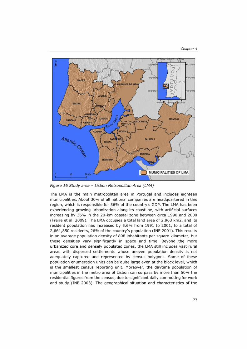
Chapter 4
77
Figure 16 Study area – Lisbon Metropolitan Area (LMA)
The LMA is the main metropolitan area in Portugal and includes eighteen
municipalities. About 30% of all national companies are headquartered in this
region, which is responsible for 36% of the country’s GDP. The LMA has been
experiencing growing urbanization along its coastline, with artificial surfaces
increasing by 36% in the 20-km coastal zone between circa 1990 and 2000
(Freire et al. 2009). The LMA occupies a total land area of 2,963 km2, and its
resident population has increased by 5.6% from 1991 to 2001, to a total of
2,661,850 residents, 26% of the country’s population (INE 2001). This results
in an average population density of 898 inhabitants per square kilometer, but
these densities vary significantly in space and time. Beyond the more
urbanized core and densely populated zones, the LMA still includes vast rural
areas with dispersed settlements whose uneven population density is not
adequately captured and represented by census polygons. Some of these
population enumeration units can be quite large even at the block level, which
is the smallest census reporting unit. Moreover, the daytime population of
municipalities in the metro area of Lisbon can surpass by more than 50% the
residential figures from the census, due to significant daily commuting for work
and study (INE 2003). The geographical situation and characteristics of the

Advancing tsunami risk assessment by improving spatio-temporal population exposure
and evacuation modeling
78
LMA, bordering the Atlantic Ocean and the large estuary of the Tagus River,
and being prone to tsunamis, provide an appropriate context for this research.
4.2.2 Data sets
The main data sets produced and used in the course of the presented analyses
were population distribution surfaces and a Tsunami Inundation Susceptibility
map (Figure 17). Input variables used for modeling population distribution
include both physiographic and statistical data.
Figure 17 Tsunami Inundation Susceptibility map for the LMA (background from Google Earth)
The first group comprises street centerlines and land use and land cover (LULC)
maps; the second set includes official census counts (INE 2001), data on
workforce, and commuting statistics (INE 2003) for the study area, produced
by Statistics Portugal. Commuting statistics were obtained in the form of an
origin/destination matrix of daily commuters at municipal level for the LMA,
from which the number of workers and students present in each municipality
was derived. The used data were obtained from various sources and in different
formats which are listed in Table 12. It was assured that all data sets were in
the same projected coordinate system. COS90 (Carta de Ocupação do Solo,
i.e., land cover map) is a digital LULC map at the scale 1:25,000 covering
almost the entire country; however, it dates from 1990. Therefore, to ensure
Chapter 4
79
near-perfect temporal consistency among input data sets, it was decided to
update it to some extent using the more recent CORINE Land Cover database
for the year 2000 (CLC2000). This updating consisted in adding the new
patches of artificial surfaces appearing between 1990 and 2000.
Table 12 Main input data sets used for modeling population distribution
Data set Source Date Data type
Street centerlines Private
vendor
2004 Vector polyline
Land use/cover maps
(COS90; CLC2000)
Public 1990;
2000
Vector polygon
Census block groups Public 2001 Vector polygon
Census statistics Public 2001 Database
(MS Access)
Commuting statistics Public 2001 Table
(O/D matrix)
Daytime worker/student
population distribution for
Cascais and Oeiras
Previous
study (Freire
2010)
2001 Raster (25 m)
The map of tsunami hazard for the LMA was produced for the Regional Plan for
Territorial Management for the Lisbon Metropolitan Area (PROTAML) report
(CCDR-LVT 2010) and was obtained in digital vector format. This map results
from modeling an event similar to the 1755 occurrence as a worst-case
scenario and depicts areas susceptible to inundation by tsunami (i.e.,
inundation extent). Susceptibility is represented using two classes or levels,
High and Moderate, with the former including low-lying coastal areas and the
latter referring to adjacent low-elevation areas farthest from the coast, with
decreasing likelihood of inundation by tsunami (Figure 17). This map can be
considered to represent maximum generic tsunami hazard for the LMA, given
that small variations in the characteristics of the tsunami source may not be
too significant for impact assessment (Lima et al. 2010).
4.3 Methodology
4.3.1 Modeling nighttime and daytime population distribution
Detailed population distribution for the LMA is modeled based on raster
dasymetric mapping using street centerlines as spatial reference units to
reallocate population counts. Dasymetric mapping is a cartographic technique
Advancing tsunami risk assessment by improving spatio-temporal population exposure
and evacuation modeling
80
which enables limiting the presence of a variable, such as population, to zones
where it is present, as defined by related ancillary data (Wright 1936). In this
model, the most recent statistical and census data available (2001) provide
the population counts to be disaggregated, while physiographic data sets are
selected and combined to define the spatial units (i.e., grid cells) used to
disaggregate those counts. The approach applied by McPherson and Brown
(2004) is combined with the innovative method of ‘intelligent dasymetric
mapping’ proposed by Mennis and Hultgren (2006) in order to transfer
population counts from original source zones to target zones. To obtain the
nighttime (residential) population distribution surface, the existing detailed
census data (INE 2001) is further refined by reallocating residential population
to effective residential areas. This procedure was initiated by identifying and
selecting strict residential land use from the updated LULC map. Two
residential classes (‘Continuous Urban Fabric’ and ‘Discontinuous Urban
Fabric’) were considered and sampled to derive the respective population
density weights, using the containment method proposed by Mennis and
Hultgren 2006. Then, eligible streets (i.e., all except freeways) were
intersected with residential land use from LULC data to obtain residential
streets, which were rasterized at 25-m resolution. Finally, the population from
census block groups (source zones) was interpolated to the respective
residential street cells (target zones) according to the density weights.
The total daytime population distribution grid results from the sum of two
surfaces on a cell-by-cell basis: (1) the daytime population in their places of
work or study—the workforce population surface—and (2) the population that
remains home during the day— the daytime residential population grid. This
latter grid is obtained by applying to the nighttime (i.e., residential), the ratio
of people who do not commute for study or work, in each municipality,
according to the population mobility statistics (INE 2003). The workforce
population surface is produced by interpolating the total number of workers
and students in each municipality (source zone) to rasterized streets within
‘labor’ and mixed ‘labor-residential’ land-use polygons (target zones). While
‘labor’ polygons were simply extracted by selecting appropriate LULC classes,
the mixed ‘labor-residential’ class was defined by applying simple rule-based
decisions to the census data and the LULC map. The empirical parameters used
for interpolation of this surface are obtained from a previous modeling effort
for part of the study area, which is based on precise geocoding of workplaces’
addresses and workforce (Freire 2010). Finally, the obtained 25-m population
density grids were aggregated to 50-m cells for subsequent analysis and
visualization purposes. Although this approach was developed and presented
in more detail in Freire and Aubrecht (2010, 2012 – Chapter 3), both the input
data and modeling rules were refined, increasing final accuracy:
Misclassification of a few areas in the LULC map were corrected, and rules used
to define the mixed ‘labor-residential’ class were improved.
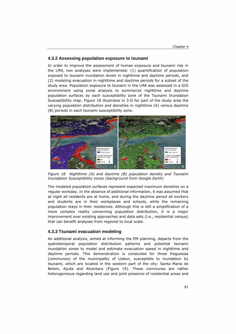
Chapter 4
81
4.3.2 Assessing population exposure to tsunami
In order to improve the assessment of human exposure and tsunami risk in
the LMA, two analyses were implemented: (1) quantification of population
exposed to tsunami inundation levels in nighttime and daytime periods, and
(2) modeling evacuation in nighttime and daytime periods for a subset of the
study area. Population exposure to tsunami in the LMA was assessed in a GIS
environment using zonal analysis to summarize nighttime and daytime
population surfaces by each susceptibility zone of the Tsunami Inundation
Susceptibility map. Figure 18 illustrates in 3-D for part of the study area the
varying population distribution and densities in nighttime (A) versus daytime
(B) periods in each tsunami susceptibility zone.
Figure 18 Nighttime (A) and daytime (B) population density and Tsunami Inundation Susceptibility zones (background from Google Earth)
The modeled population surfaces represent expected maximum densities on a
regular workday. In the absence of additional information, it was assumed that
at night all residents are at home, and during the daytime period all workers
and students are in their workplaces and schools, while the remaining
population stays in their residences. Although this is still a simplification of a
more complex reality concerning population distribution, it is a major
improvement over existing approaches and data sets (i.e., residential census)
that can benefit analyses from regional to local scale.
4.3.3 Tsunami evacuation modeling
An additional analysis, aimed at informing the EM planning, departs from the
spatiotemporal population distribution patterns and potential tsunami
inundation zones to model and estimate evacuation speed in nighttime and
daytime periods. This demonstration is conducted for three freguesias
(communes) of the municipality of Lisbon, susceptible to inundation by
tsunami, which are located in the western part of the city: Santa Maria de
Belem, Ajuda and Alcantara (Figure 19). These communes are rather
heterogeneous regarding land use and joint presence of residential areas and

Advancing tsunami risk assessment by improving spatio-temporal population exposure
and evacuation modeling
82
economic activities, therefore providing a good test bed for this demonstration.
The evacuation analysis assesses the time needed, after a full evacuation is
initiated, for the population to reach safe areas, that is, areas immediately
outside of the inundated zone, assuming they are traveling by foot. Part of the
methodology was developed in the framework of the German-Indonesian
Tsunami Early Warning System (GITEWS) project (Post et al. 2009; Strunz et
al. 2011; Wegscheider et al. 2011). The evacuation modeling is performed
using GIS-based geospatial analysis and relies on a cost-weighted distance
approach. The best (i.e., the fastest) evacuation route from any given location
to a safe area is defined, and the time needed to reach it is calculated.
Figure 19 Study area for Tsunami evacuation modeling
The output of the model, that is, the time needed for evacuation toward a safe
area, is based on several parameters: (1) extent of the hazard impact area
(i.e., potential inundation area), (2) characteristics of the evacuation paths
(slope, land cover, street network), (3) (time-specific) population density and
(4) location of critical facilities (i.e., facilities with people of reduced or lacking
abilities to evacuate, such as hospitals). For more details see Post et al. (2009)
and Wegscheider et al. (2011). Data from the Urban Atlas
(www.eea.europa.eu/data-and-maps/data/urban-atlas) that recently became
available were used as source of land cover information. The Urban Atlas
project maps land cover and land use for selected European cities (i.e.,
including the part of the LMA chosen for the tsunami evacuation modeling case
study) using 19 thematic classes and has a minimum mapping unit of 0.25 ha

Chapter 4
83
(for ‘Artificial surfaces’). While not being available for the entire LMA, it is a
more detailed and updated source of LULC info for intra-urban analysis than
COS90 + CLC2000. The derived evacuation time surfaces are used, in
combination with the detailed population distribution grids, to calculate the
number of successful evacuees after certain time intervals.
4.4 Results and discussion Using the above-described intelligent dasymetric mapping methodology, four
raster population distribution surfaces were produced, at 50 m resolution: (1)
nighttime (residential) population, (2) daytime residential population, (3)
daytime worker and student population, and (4) total daytime population. The
nighttime population distribution is finer than the one provided by the original
census data, and the other three population grids were previously unavailable.
The new nighttime and workforce distribution grids were validated using
correlation analysis with higher-resolution reference data, that is, block-level
census and the previous’ model distribution for Oeiras, respectively.
Correlation coefficients (Pearson’s r) of 0.86 and 0.64, respectively, were
obtained for each of these two population grids.
Concerning the population distribution model, an additional source of
uncertainties lies in the spatial nature and dynamic character of activities used
to produce the daytime worker and student population grid, combined with the
unavailability of mobility statistics more detailed than at the municipal level.
Still, the usefulness of earlier versions of similar spatio-temporal population
distribution surfaces for the LMA, which are multi-purpose, was illustrated for
Disaster Risk Management applications, specifically in improving earthquake
risk assessment (Freire and Aubrecht 2010, 2012). Population surfaces at such
high resolution prove more appropriate for local-level quantification of human
exposure, enabling a more detailed and thorough assessment of potential
effects and impacts. Results of the analysis of exposure to tsunami in the LMA
show that the population potentially exposed to some level of tsunami
inundation hazard significantly increases from nighttime to daytime periods
(Table 13). The majority of the population exposed is associated with the ‘high
inundation susceptibility’ zone. Particularly these ‘high hazard’ areas also
feature a significant increase in population from nighttime to daytime, both in
absolute and in relative terms (i.e., as proportion of total population within the
inundation zone). While during nighttime around 60% of the potentially
exposed population is located in areas having a high tsunami hazard level,
daytime population movement results in more than 200,000 persons
additionally exposed in that area, corresponding to a factor of increase greater
than 2.5. Considering the total population of the Lisbon Metropolitan Area, 16%
of the daytime population is potentially exposed, compared to 8% of the
resident population during the nighttime period. While population exposure to
the moderate hazard level remains relatively stable at 3%, a considerable

Advancing tsunami risk assessment by improving spatio-temporal population exposure
and evacuation modeling
84
increase from 5% during nighttime to 12% during daytime is observed in the
highly susceptible areas. These results reflect the location of human economic
activities closer to the coastline and highlight the more intensive occupation of
these areas during the daytime period.
Table 13 Population exposed to Tsunami inundation levels in nighttime and daytime periods in the LMA
Tsunami hazard Population
[Inundation levels] Abs.
[Pers.]
Rel.
[%]
High 125,730 59 Nig
ht
Moderate 86,929 41
Total 212,659 100
High 334,000 78
Day
Moderate 93,444 22
Total 427,444 100
High 208,270 166 Diffe
r.
Moderate 6,515 7
Total 214,785 101
*Relative differences are relative to the night
numbers
Regarding the modeling of tsunami evacuation, Figure 20 shows the modeled
surfaces of evacuation time and access points to safe areas (i.e., outside of the
inundation zone), for the nighttime (A) and daytime (B) periods, respectively.
The differences for nighttime and daytime evacuation times become intensified
by the fact that densely populated areas are slower to evacuate, as a higher
‘traffic volume’ of evacuees slows down the speed of every individual (Klupfel
2005; Rogsch 2005). This is also considered in the modeling process.
Therefore, longer evacuation periods are observed in daytime, since about
40,000 people are estimated to be present in the hazard zone in the three
communes in this period, compared to 8,000 residents in nighttime.

Chapter 4
85
Figure 20 Nighttime (A) and daytime (B) Tsunami evacuation modeling
Results of the evacuation modeling analysis reveal significant differences in the
magnitude and speed of evacuation between night and day (Table 14).
Differences are especially striking in the commune of Alcantara, due to the
configuration of hazard zone and population distribution. Overall in the study
area, all resident (nighttime) population is able to evacuate to safety within 10
min. In daytime, although more than 95% of the population has reached safety
after 20 min, it takes as long as 90 min for a full evacuation. This duration is
longer than the travel time to this location for the devastating 1755 tsunami
(approx. 50–70 min; Baptista et al. 1998), implying that for a similar scenario,
there could be approximately 700 people in the study area who would not reach
safe areas on foot, according to the modeled results. This is assuming that
everyone present in the hazard zone would initiate evacuation to closest safe
areas immediately following a large earthquake (greater than M = 6.5) or
tsunami warning, but no early-warning and evacuation system for tsunamis is
yet implemented in Lisbon. Therefore, it would be important to consider other
safety measures, such as vertical evacuation, that would shorten travel time
to safety. Also, this analysis would be improved by further considering
nonresidents and nonstudents/workers (e.g., tourists) present and involved in
leisure activities, which are especially relevant in the Alcantara (nightlife) and
in the Belem (daytime museums and monuments) communes. For this
exercise, we are not considering the specific effects in the area that a triggering
earthquake might cause in people, buildings and other structures, impacting
the ensuing evacuation from tsunami, since such a detailed and spatially
explicit modeling is not available.
Table 14 Population remaining in hazard zone and successful evacuees after different time intervals of tsunami evacuation
Commune Elapsed
time
Population
[min] Remaining Evacuees

Advancing tsunami risk assessment by improving spatio-temporal population exposure
and evacuation modeling
86
Santa
Maria de
Belém
0 4,300 0 Nig
ht
5 1,600 2,700
10 0 4,300
Santa
Maria de
Belém
0 25,800 0
Day
5 19,900 5,900
10 4,600 21,200
15 500 25,300
20 400 25,400
75 0 25,800
Alcântara
0 3,800 0 Nig
ht
5 300 3,500
10 0 3,800
Alcântara
0 17,700 0
Day
5 9,200 8,500
10 900 16,800
15 200 17,500
20 200 17,500
90 0 17,700
Ajuda 0 200 0
Nig
ht 5 0 200
Ajuda 0 200 0 D
ay 5 0 200
4.5 Conclusions and outlook This work is an initial approach toward considering the spatio-temporal
population distribution to assess risk of tsunami in a large metropolitan area.
The region is prone to this hazard and was severely affected by this type of
event in the past. Improved high-resolution data sets of nighttime and daytime
population density were developed and combined with existing Tsunami
Inundation Susceptibility zones to estimate potential population exposure in
those periods in the Lisbon Metropolitan Area. In addition, evacuation speed
was modeled and analyzed for both scenarios in a subset of the study area.
Results show that potential population exposure to tsunami is significantly
time-dependent, displaying a strong variation from nighttime to daytime. The

Chapter 4
87
analysis indicates that a significant amount of population is at risk, and its
numbers increase dramatically from nighttime to daytime, especially in the
zones of high susceptibility (i.e., lower elevation and closer to the coastline).
Evacuation modeling reveals that full horizontal evacuation may be problematic
in the daytime period, even if initiated immediately after an early warning or a
major tsunami-triggering earthquake event. This finding recommends that
additional measures be considered as alternatives, such as vertical evacuation.
As with any similar exercise, this model implies a number of uncertainties that
can affect the specific results of population distribution, exposure and
evacuation. However, the analyses provide valuable information for further
development of scenarios leading to evacuation planning and management
measures, yet to be implemented in the study area. This improved
characterization of vulnerability and risk can benefit all phases of the disaster
management process where human exposure should be considered, namely in
emergency planning, risk mitigation, preparedness and response to an event.
Considering the large variations between nighttime and daytime population
exposure that become apparent in the presented case study model, it is clear
that integration of this kind of information in a pre-event assessment stage
would favor preparation for actual hazardous events and thus be a huge step
toward improved mitigation and eventually saving lives. The new population
surfaces can also be used as input in loss simulators for modeling of human
casualties resulting from different types of hazards and threats, such as
earthquakes, flash floods, landslides or chemical accidents. Given the
availability of input data sets, this approach could, for example, also be applied
to the Oporto Metropolitan Area, further encompassing nine municipalities and
1,260,680 inhabitants.
Planned future developments include conducting a more detailed spatial
modeling of population distribution and exposure assessment to tsunami at the
building level considering its function, height and elevation (Aubrecht et al.
2010). This will also enable modeling of vertical evacuation, that is, evacuation
to a safe structure or floor above the inundation level. Subsequent analyses
would also benefit from assessing likely population exposure in additional
temporal cycles, relevant for population dynamics in large urban centers (e.g.,
rush hour, week-ends, etc.). Especially useful for tsunami risk assessment
would be to account for seasonal differences, given that human occupation of
beaches is usually very high in warm summer days.
Acknowledgments:
The authors thank Prof. J. L. Zezere and the RISKam group (CEG-IGOT) for
providing the tsunami inundation susceptibility map.

Advancing tsunami risk assessment by improving spatio-temporal population exposure
and evacuation modeling
88

89
Chapter 5. Enhanced data and methods
for improving open and free global
population grids: putting ‘leaving no
one behind’ into practice37
37 This chapter is published as:
Freire S., M. Schiavina, A. J. Florczyk, K. MacManus, M. Pesaresi, C. Corbane, O. Borkovska, J. Mills, L. Pistolesi, J. Squires & R. Sliuzas, 2018. Enhanced data and methods for improving open and free global population grids: putting ‘leaving no one behind’ into practice. International Journal of Digital Earth, 13:1. DOI: 10.1080/17538947.2018.1548656

Enhanced data and methods for improving open and free global population grids: putting
‘leaving no one behind’ into practice
90
Abstract Data on global population distribution are a strategic resource currently in high
demand in an age of new Development Agendas that call for universal
inclusiveness of people. However, quality, detail, and age of census data varies
significantly by country and suffers from shortcomings that propagate to
derived population grids and their applications. In this work, the improved
capabilities of recent remote sensing-derived global settlement data to detect
and mitigate major discrepancies with census data is explored. Open layers
mapping builtup presence were used to revise census units deemed as
‘unpopulated’ and to harmonize population distribution along coastlines.
Automated procedures to detect and mitigate these anomalies, while
minimizing changes to census geometry, preserving the regional distribution
of population, and the overall counts were developed, tested, and applied. The
two procedures employed for the detection of deficiencies in global census data
obtained high rates of true positives, after verification and validation. Results
also show that the targeted anomalies were significantly mitigated and are
encouraging for further uses of free and open geospatial data derived from
remote sensing in complementing and improving conventional sources of
fundamental population statistics.
5.1 Introduction Accurate geospatial data on global population distribution and characteristics
are increasingly required and relied upon for analysis and modelling in an
expanding range of disciplines (Gaughan et al. 2014; Wardrop et al. 2018).
These data are also crucial in the frame of the Digital Earth perspective in the
path towards decision-making (Shupeng and van Genderen 2008). In the
context of evidence-based assessment for policy support, the recent wave of
post-2015 international development agreements (including the Sendai
Framework for Disaster Risk Reduction 2015–2030 (adopted March 2015);
United Nations (UN) 2030 Agenda for Sustainable Development (SDGs,
September 2015); COP 21 Paris Agreement on Climate Change (November
2016); UN New Urban Agenda (December 2016)) places great demands and
responsibility on geospatial data, and in particular on that related to
population.
Public information about the characteristics and spatial distribution of
population is a strategic resource supporting the monitoring and
implementation of international frameworks. Information about population
density per uniform spatial sampling schemas (e.g. grid cells) are necessary
for modelling critical aspects of human-environment interaction, such as:
Exposure (to hazards, pollutants); Access (to resources, services, facilities);
and Impacts, in both perspectives of (i) the impact of human activities on the
planet and (ii) impact of the environment on the people living on the Earth’s
surface (natural disasters, environmental change) (UNISDR 2015a; UNDESA

Chapter 5
91
2016; UNECOSOC 2016). The Sustainable Development Goals (SDG) indicators
are ‘action oriented, global in nature and universally applicable’ and should be
themselves sustainable and comparable across space and time (UNECOSOC
2016, 7). Ideally, the indicators supporting the international development
agenda should be based on geospatial population data that is up-to-date,
sufficiently detailed, accurate, consistent, cost-effective (i.e. sustainable),
transparent (i.e. using clear methods), and accessible to all. These
development agreements, their targets and monitoring needs (i.e. indicators)
present an opportunity not only for producing more data, but also for improving
existing datasets. The reliability of international statistics is periodically called
into question (e.g. Wolff, Chong, and Auffhammer 2011), and the recent surge
in initiatives aimed at producing more accurate and detailed statistics (e.g. by
UN (UNDP 2018), World Bank (WB 2018), Bill & Melinda Gates Foundation and
UK Department of International Development) are a realization that statistical
capacity must be strengthened (UNECOSOC 2016).
Regular grids (raster or vector) are now well established and widely used
spatial structures to model and report population attributes, and their
advantages are largely recognized (Deichmann, Balk, and Yetman 2001).
Several global gridded population datasets are currently produced. They are
differentiated by the underlying population concept (e.g. ‘resident’ vs.
‘ambient’ population), gridding method, and distribution policy (for reviews and
recent developments see Linard and Tatem 2012; Stevens et al. 2015; Freire
et al. 2016a). For a given spatial unit, population distribution grids can be
produced by disaggregating (e.g. gridding) population counts (top-down
approach) or by estimating that count at the grid cell level through combining
sampling with ancillary data (bottom-up method) (Wardrop et al. 2018). Global
population grids aiming to support policies and international agreements in
global forums are typically based on available statistics whose national totals
match, or are adjusted to match, those used in UN population estimates (e.g.
UNDESA 2015). UN estimates are used as a standard in order to produce more
accurate and harmonized datasets for countries where census data are
considered to be less reliable, and because of the extensive work done by the
UN Population Division to adjust and correct census data post enumeration.
Examples of such grids include Gridded Population of the World (GPW)
(Deichmann, Balk, and Yetman 2001; Doxsey-Whitfield et al. 2015) the Global
Rural-Urban Mapping Project (GRUMP) (Balk et al. 2006), and the Global
Human Settlement Population (GHS-POP) (Freire et al. 2016a). For population
grids that are generated by disaggregating available statistics (top-down) while
preserving their volume, output accuracy (with respect to ground truth data)
is largely dependent on the spatial detail and quality of input geospatial layers.
In addition to their spatial detail, population census-like layers vary widely in
quality concerning their geometry, attributes, reliability, and currency.
Incidentally and unfortunately, the quality and reliability of statistics’ are

Enhanced data and methods for improving open and free global population grids: putting
‘leaving no one behind’ into practice
92
particularly low in many developing countries (Tatem et al. 2007), at whom
the post-2015 development agenda is especially directed.
Production of global grids relies on population sources that are somewhat
heterogeneous in respect to these characteristics. These sources include
provisional or final censuses originating in National Statistical Offices (NSOs)
as well as estimates and projections provided by Non-governmental (NGOs)
and other organizations. Despite valuable efforts to collect, integrate, and
improve global census data obtained from disparate sources (e.g. GPW), some
important requirements remain unsolved. Addressing the universal
inclusiveness requisite associated with the UN ‘leaving no one behind’
imperative of the new sustainable development agenda (UNDESA 2016)
requires that all people are counted and accounted for in the place they live.
However, census enumerations often do not meet this requirement (even
sometimes by design as in de facto census), and any statistical sampling
inherently lacks information about marginal and uncounted populations.
Perhaps surprising and unknown to some users, available population statistics
also suffer from error and uncertainty that affect even the most basic of
demographic variables (i.e. total population). While uncertainty is difficult to
assess and communicate, error often propagates unimpeded to downstream
analyses and applications. The main deficiencies and shortcomings affecting
geospatial population statistics can be summarized in the following basic
taxonomy:
1. Issues affecting geography (census reporting units): a) Lack of spatial detail
(i.e. too coarse or generalized, related to spatial precision) b) Low spatial
accuracy (i.e. units partially displaced or completely misplaced)
2. Issues affecting attributes (population counts in present case) a)
Undercounting and/or underreporting (i.e. underenumeration) b) Over-
counting and/or over-reporting (i.e. overenumeration)
These issues have been unnoticed or unaddressed due to the lack of external
accuracy assessment related to a shortage in independent compatible high-
resolution reference data. Notable exceptions are the works of Hay et al.
(2005) and Mondal and Tatem (2012) that discuss deficiencies in the
representation of population distribution along coastlines, and Linard and
Tatem (2012) that address these in frame of infectious disease research. In
contrast to remote sensing-based maps where validation is expected to rely on
independent reference data, typically collected from ground truthing (see
Congalton and Green 2009), quality assessment of population grids is usually
limited to internal consistency of model performance (i.e. population data used
for validation is the same that was used for modelling, just finer). Also, the
relative coarse resolution of global grids produced until recently (i.e. ∼1–5 km)
mitigated the impact of some deficiencies that now become apparent as cell
sizes approach ∼100 m.

Chapter 5
93
Significant improvements to the quality of population grids are to be gained by
addressing some of these shortcomings. Detection and mitigation of
deficiencies in population statistics require independent, reliable, higher-
resolution data. Remote sensing imagery and methods have been evolving
towards constituting a more detailed, objective and independent data source
on human presence on the Earth surface. The combination of new cost-
effective, automated and fully replicable data classification methods (e.g.
machine learning) with the synoptic capacities of satellite Earth Observation
imagery, made accessible in a public, full open-and-free frame, can contribute
to fill information gaps and supplement existing statistics by mitigating some
major shortcomings in population data. This is especially true in poor, remote,
unsafe, disputed, very large, and/or highly dynamic areas of the globe where
conventional data gathering and updating is challenging.
Current methods and processing capacity allow for global mapping of built-up
areas and settlements with unprecedented spatio-temporal detail and accuracy
– in essence capturing the local scale with global coverage, finally starting to
fulfil a long-standing promise of remote sensing technology. Making these
datasets available open and free helps to increase access, promotes
transparency, and ensures accountability of the information produced. Global,
consistent and updated geospatial data such as that made openly available in
the framework of the Global Human Settlement Layer (GHSL) (Pesaresi and
Ehrlich 2009) are already providing an effective contribution and improving the
disaggregation of census data into derived population grids (Freire et al.
2015d; Linard et al. 2017; Nieves et al. 2017). However, it remains to be
tested in large scale if such remotely sensed data can also assist in assessing
and mitigating major deficiencies present in geospatial population statistics.
This article addresses shortcomings present in global collections of census
data, by introducing, applying, and discussing novel procedures aimed at
investigating and detecting some of those major anomalies. It then
demonstrates mitigation of some inconsistencies using high-resolution
geospatial data derived from remote sensing. The focus is on deficiencies in
mapping coastlines and declared unpopulated areas, as extreme instances of
deficiencies 1a) and 1b) and 2a) in the taxonomy mentioned above. Making
use of open and free high-resolution global settlement layers derived from
contemporary satellite imagery, the approaches are illustrated with GHSL in
the frame of producing GHSL-based new global population grids (release
2018).
5.2 Materials and methods Two main types of geospatial data were used in this work: vector-based census
data reporting on estimated total population counts for the target year of 2015
(http://sedac.ciesin.columbia.edu/ gpw), and raster layers reporting on built-
up presence for 2013/2014 derived from Landsat image collections in the

Enhanced data and methods for improving open and free global population grids: putting
‘leaving no one behind’ into practice
94
frame of the GHSL project (http://ghslsys.jrc.ec.europa.eu/index.php). Some
aspects of these two datasets are compared and combined, with remote
sensing data being used to identify anomalies in the geospatial census data.
These anomalies are mitigated with the support of the remote sensing-derived
data after verification and validation.
5.2.1 Data sets
5.2.1.1 Geospatial data on census population
As a source of census population data, a database assembled by the Center for
International Earth Science Information Network (CIESIN) in the frame of the
Gridded Population of the World project (Tobler et al. 1997) was used. For
more than two decades, GPW has been collecting, combining, and harmonizing
available population census and estimates into what is considered the most
complete, detailed and coherent census-based geodatabase available globally.
This database is periodically updated with more recent and improved data, with
GPW employing clear and transparent methods to create open and free
residence-based population grids for different reference years (Doxsey-
Whitfield et al. 2015). Despite these efforts, the GPW databases are subject to
availability and quality of source (national) population statistics, and therefore
inherit their gaps and shortcomings, as reliability and currency of population
data is quite heterogeneous among countries (for GPW metadata see CIESIN
2017a).
The GPW data used consisted in country-based layers (one for each of 241
countries) of census and administrative polygons containing estimated
residential population for the GHSL target years 1975-1990-2000-2015,
adjusted to country-level estimates of UN World Population Prospects 2015
(UNDESA 2015). Due to the development of the work and the updating
schedule of GPW data, two versions from the same release were used: GPWv4,
released in 2016 (CIESIN 2016), was used for detection of inconsistencies
along coastlines; GPWv4.10, available in late 2017 (CIESIN 2017b), was used
for revision of unpopulated areas. GPWv4.10 is a revision of GPWv4 with
boundary or population updates for 64 countries. More details about these data
can be found here: http:// sedac.ciesin.columbia.edu/data/collection/gpw-v4.
5.2.1.2 Built-up areas from remote sensing
In the frame of the Global Human Settlement Layer (GHSL) project, global
built-up (BU) areas were recently mapped with unprecedented spatial detail,
consistency, and temporal coverage (Pesaresi et al. 2016). The GHSL has
developed and employed novel and automated approaches to produce a time
series of raster layers reporting on the presence of building structures, defined
as ‘all constructions above ground intended for human or animal sheltering or
for the production of economic goods’ (Pesaresi et al. 2013). These data were
derived from Landsat image collections spanning four periods: 1975, 1990,

Chapter 5
95
2000 and 2013–2014 and are made available open and free. Quality assurance
was conducted to validate these data against a heterogeneous set of available
layers mapping building footprints (Pesaresi et al. 2016). More recently,
independent spatio-temporal quality assessment of the GHSL built-up time
series was performed for the USA showing very encouraging accuracy that
generally increases over time (Leyk et al. 2018). Most relevant for the present
work, these built-up areas exhibited strong correlation with population
distribution and density, and suitability for population disaggregation and
modelling (Freire et al. 2015d, 2016; Linard et al. 2017; Nieves et al. 2017).
In this effort, global layers mapping built-up areas for the latest epoch (2013–
2014), at spatial resolutions of 38 and 250 m, were used as an indication of
the presence of human settlements. Due to the development timeline of this
work and the updating schedule of GHSL products, data from different releases
were used: the GHS-BUILT data released in 2015 (GHS_BUILT_LDSMT_GLO-
BE_R2015B) were used for combination with census data from GPW for initial
flagging and systematic detection of discrepancies (Pesaresi et al. 2015a);
while the latest and improved GHSBUILT data
(GHS_BUILT_LDSMT_GLOBE_R2018A), produced in Fall 2017 (Corbane et al.
2017), to be publicly released in Fall 2018, were used for population
disaggregation and creation of final population grids. All geospatial layers were
projected to World Mollweide projection (EPSG 54009), the equal-area
projection adopted for production of the GHSL global population grids. This is
also important for the processing undertaken and described here, which is
mostly based in quantification and comparison of surfaces.
5.2.2. Revision of ‘unpopulated’ units
An extreme case of issue 2a) of the taxonomy of census anomalies proposed
in Section 1. is the reporting of areas as ‘unpopulated’ or ‘uninhabited’ or
otherwise as containing no population. During the early stages of production
of GHSL global population grids, it was observed that some units declared as
having no population in census data in fact contained settlements and
significant areas of built-up according to the GHS-BUILT data. Consequently a
spatial analysis procedure was designed to (i) check for the presence of
(resident) population in census units where no population was reported, and
(ii) mitigate these issues while minimizing changes to the input census data
(conservative approach). Units deemed as ‘uninhabited’ or otherwise
unpopulated in the census data were critically assessed for the presence of
significant residential population, based on ancillary data (e.g. coordinates of
populated places) and very high resolution (VHR) imagery. Such census units
were then selected based on their size and the extent of built-up surface in
2014 as an indication of the likely presence of settlements. Due to the
experimental nature of the work, a sequential approach was adopted in order
to inspect, control, and calibrate the assumptions made at each step. Adopting

Enhanced data and methods for improving open and free global population grids: putting
‘leaving no one behind’ into practice
96
a conservative approach was important to quickly narrow the selection to the
main issues and limit the rate of false positives. For selection of potentially
problematic census units, a simple semi-heuristic rule-based approach was
followed. From the set of census units in GPWv4.10 having no population
(238,029 units), most non-residential zones were filtered out by selecting
polygons larger than 300 ha (3 km2). This threshold was adopted because it
is the mean size of non-residential built-up patches (i.e. industrial, commercial,
and service facilities) in the CORINE Land Cover (CLC) 2012 vector map,
v18.5.1 (EEA 2016). CLC2012 currently covers 39 countries and 5.8M km2 in
Europe, and this threshold may not be the best one to use in other contexts.
From these 47,508 census units larger than 300 ha, units were selected that
contained a total surface of built-up in 2014 (according to GHS-BUILT R2015B)
greater than 10 ha, to increase confidence in presence of significant resident
populations. As the resulting set of 2,717 units was still too large a number for
visual inspection with available resources, and after confirming it would include
a high rate of false positives in countries that have both detailed and accurate
censuses, countries deemed, based on our in-depth empirical knowledge of the
data, as having reliable census (14 of the 45 countries in set) were excluded.
This led to the identification of potentially problematic census units in 31
countries, to be visually inspected for verification and validation of the
approach. These units were inspected using VHR imagery from web mapping
services (Esri World Imagery service through the ArcMap application). After
collecting sufficient visual evidence that some units were inhabited (i.e.
presence of residential-type buildings with signs of habitation), that anomaly
had to be mitigated. A decision was taken to adopt the most conservative
approach that would imply minimal changes to the GPW’s geospatial census
dataset and still ensure that some population would be accounted in those
areas, to be then disaggregated to the mapped BU areas in the creation of
GHS-POP grids. To implement this, a ‘smart’ geoprocessing approach was
devised and automated (hereafter called ‘split and merge’) to assign population
to those previously unpopulated areas without altering the boundaries and the
total population of the upper administrative level. The approach involves
splitting and merging the confirmed problematic polygons, based on
geographical proximity to those ones adjacent and containing population, and
merging the split parts to the latter.
Figure 21 shows the main steps involved in the application of the ‘split and
merge’ approach. This method consists in spatially dividing the problematic
polygons according to a proximity rule accounting for adjacent populated
polygons belonging to the same administrative unit. This task is performed by
(i) re-projecting the polygons to an equidistant projection, more suitable for
measuring distances (i.e. World Equidistant Cylindrical), (ii) rasterizing to a
sufficiently fine resolution (i.e. a trade-off between accuracy and computational
demand) with an all-touched approach, (iii) applying a nearest-neighbour

Chapter 5
97
nibbling technique (only considering populated neighbouring units), (iv)
polygonising the resulting part and finally (v) re-projecting back to the original
projection. The polygons obtained are then cleaned of geometric artefacts by
clipping them to the original boundary. Each generated part of the problematic
polygon is then dissolved with the related populated neighbouring unit, in this
way ‘populating’ the whole original problematic area.
Figure 21 Flow chart of the ‘split and merge’ approach
5.2.3 Harmonization of population and settlement data along coastlines
Seashores and waterfronts can be especially intense and dynamic zones, due
both to natural processes and their attractiveness for settlement and building
of infrastructure (EEA 2006; McGranahan, Balk, and Anderson 2007; Freire,
Santos, and Tenedório 2009). These strong and fast dynamics contribute to
making census or administrative geometries outdated or inaccurate. Moreover,
the geospatial census data are not produced with globally harmonized technical
specifications, thus including different nominal scales and spatial tolerance
characteristics. The characteristics of the GHSL layer mapping built-up areas
(i.e. seamless coverage, uniform technical specs, decametric-scale spatial
detail, currency) have revealed discrepancies with GPW along coastlines
(including inland water bodies). Most of these consisted in the coastline from
GPW being inland respect to that actually detected by GHSL, implying in
practice that no population would be disaggregated to those mapped built-up
areas in GHSL that were water bodies in GPW (i.e. spatial mismatch between
source and target zone). This would cause changes to the population density

Enhanced data and methods for improving open and free global population grids: putting
‘leaving no one behind’ into practice
98
and extent of coastal settlements or omit them entirely in the resulting
population grids. Therefore, a systematic procedure was developed aiming at
identifying globally the main inconsistencies between the two datasets along
coastlines, and efforts were undertaken to reconcile them. This procedure was
aimed at harmonizing population and settlement data along coastlines, but
does not intend to harmonize the delineation of water bodies themselves. The
high-resolution (38 m) GHSL layer on built-up areas for 2014 (GHS-BUILT from
R2015B), available at the time of work, was used to detect the significant
human presence (i.e. BU) beyond GPWv4 censuses coastlines. The process of
detecting inconsistencies included the following three main steps: (i) creation
of a layer depicting the built-up areas outside of the GPW landmass, (ii)
identification of potentially inhabited patches containing built-up, and (iii)
visual inspection and validation of the patches. It is well known that full
automatic detection of built-up areas from satellite imagery is prone to com-
mission errors in sandy or rocky landscapes, and, as a result, part of the built-
up area pixels in coastal areas might be false positives. Therefore, a visual
inspection was required. It should be noted that the term coastline here refers
to inland water bodies as well as seashores, and the level of detail at which
coasts are outlined varies widely across countries (e.g. the inland water bodies
in the USA are depicted with high detail while in most other countries only the
large ones are outlined with low detail).
During step (i), first a water mask derived from the country polygons of GPWv4
data was rasterized at approximately 38 m, and only within the data domain
of the GHSL layer as defined by the GHSL Datamask product (Pesaresi et al.
2015b). Then, this coastal water layer was intersected with the GHS-BUILT
layer, producing the built-up areas not overlapping with any GPW country poly-
gons. In total, these areas have amounted to 6,142 km2 of surface. The
procedure for selecting and validating potentially inconsistent patches included
three steps: (1) vectorizing connected cells classified as built-up surface (using
4-connectivity rule) into individual polygons (nearly 800,000 patches, with a
mean surface of 7700 m2, corresponding to 5/6 contiguous pixels), (2)
selecting all patches larger than 1 km2 (287 selected), and (3) visual inspection
using GIS software and very high resolution (VHR) satellite imagery from web
mapping service (Google Maps) to confirm presence of buildings. The 1 km2
size threshold was chosen to balance importance and potential impact of
inconsistencies with resources available for verification and validation. Figure
22 shows examples of built-up patches located beyond the coastline of GPW in
Japan, Tunisia, China, and Romania, assessed during visual inspection. For the
selected patches (those larger than 1 km2) in which visual inspection
confirmed presence of built-up surfaces, mitigation consisted in reconciling the
outline of GPW census units with built-up patches by manually extending the
units on the coast to include these areas.

Chapter 5
99
Figure 22 Examples of detected discrepancies (patches larger than 1 km2) between GPWv4 (blue line) and GHS-BUILT 2014 (orange) along the coasts of (A) Japan (JPN), (B) Tunisia (TUN), (C) China (CHN), and (D) Romania (ROU)
After conducting automatic detection and during visual inspection of the main
coastal discrepancies between GPWv4 and GHSL, systematic or additional
inconsistences were identified. These systematic inconsistencies between the
more recent and improved GHS-BUILT P2018 and GPW4.10 layers were still
present in some countries: Japan, Ukraine, Switzerland, and France. Therefore,
an automated approach to mitigate these issues that appear to be caused by
the coarser scale (low spatial detail) and/or positional errors (poor
georeferencing) of census reporting units was developed and applied. For
inconsistences detected in lakes (i.e. Switzerland and France) the ‘split and
merge’ approach (described in Section 2.1) was directly applied to polygons
representing lakes in order to split them and dissolve each part with the
nearest neighbour polygon. In coastal areas, such as in Ukraine and Japan, the
GPW coastline was first extended seawards using a 2-km external buffer. Next,

Enhanced data and methods for improving open and free global population grids: putting
‘leaving no one behind’ into practice
100
this buffer was split according to proximity to the original census units by using
the split and merge approach, and then assigned each part of the buffer to a
census polygon (see Figure 28). In this case, the whole set of census polygons
was used, without selecting only the populated areas.
5.3 Results and discussion
5.3.1 Revision of unpopulated units
The implementation of the semi-automated rule-based procedure to the initial
238,029 census units deemed as uninhabited in GPW geospatial census data
resulted in the selection of 128 units in 31 countries as potentially containing
significant resident population (Figure 23).
Figure 23 Global distribution of census units without population in GPWv4.10 data and those flagged based on the automated procedure developed (USA not considered). Note that existence of unpopulated units is merely a feature of census design and not of the landscape
All of these 128 units were validated visually with VHR imagery from web
mapping services (Esri/Bing, Google maps). This was both to proceed with
confidence in such a sensitive issue, and to assess the validity of the semi-
heuristic rule-based approach used for selection of problematic units. The
validation with VHR imagery revealed the presence of significant residential
areas having clear signs of habitation in 76 census units, belonging to 19
countries (Table 15), resulting in a success rate of the automated procedure of
around 59% (of polygons). These 76 problematic units have a combined area
of 297,090 km2, of which 624 km2 are reported by GHSL to be covered by
building structures in 2014. If this built-up surface is accurate and all of it is
dedicated to residential function, using a low occupancy rate of 100 m2 of built-
up surface per person would put a conservative estimate of under-reported

Chapter 5
101
population in these units at more than 6 million people. Some recent estimates
put the value of ‘missing’ (i.e. undercounted) people in urban slums at 369
million worldwide (Carr-Hill 2017).
Table 15 List of countries in which problematic polygons were selected
Country N Area
(km2)
BU area 2014
(km2)
Afghanistan 1 76.7 0.1 Armenia 1 53.2 2.0 Democratic Republic of the Congo
7 99,575.9 154.9
Colombia 1 514.1 0.1
Cyprus 1 4.4 0.4 Egypt 16 184,254.7 283.2 Georgia 2 2005.2 1.8 Guyana 1 918.6 0.7 India 1 116.4 70.3 Iraq 4 8459.9 65.7 Lebanon 4 56.1 0.7
Mali 2 53.5 14.0 Malawi 14 121.1 4.7 Nepal 1 163.9 1.7 Philippines 1 86.6 0.9 Rwanda 1 37.7 0.2 Serbia 16 214.5 7.5
Thailand 1 306.4 2.1 Ukraine 1 71.1 12.6
Total 76 297,090 623.7
Note: For each country the number of polygons (N), the sum of the area of such polygons and the total built-up (BU) surface accounted by GHSL built-
up layer in 2014 is reported. Mitigation of these anomalies was carried out using the ‘split and merge’
approach, which was applied to a total of 58 units covering about 296,670
km2, in the following countries: Afghanistan, Armenia, Democratic Republic of
the Congo (DRC), Colombia, Cyprus, Egypt, Georgia, Guyana, Iraq, Lebanon,
Mali, Malawi, Nepal, Rwanda, Thailand, and Ukraine. Among them, the
Democratic Republic of the Congo and Egypt are the most problematic, with
the surface of incorrectly labelled ‘unpopulated’ units reaching 99,576 km2 and
184,255 km2, respectively. In Egypt some problems seem to be caused by the
coarse spatial detail and spatial inaccuracy of census polygons.
Figure 24 shows the results of the application of the ‘split and merge’ approach
in Guyana and Lebanon. In Guyana, the declared unpopulated polygon (Figure
24 (A1)) is split into seven parts and is then dissolved with adjacent polygons
belonging to the same administrative level (Figure 24 (A2)). In Lebanon the
setting is more complex: the target polygon (Figure 24(B1)) is split into four
parts which are then dissolved with the neighbouring administrative units,

Enhanced data and methods for improving open and free global population grids: putting
‘leaving no one behind’ into practice
102
three of which are to the East of a unit (in grey) correctly declared as
uninhabited. The resulting polygons, preserving their respective population
counts, replace the problematic one in the census database that is used as one
of the inputs (source zones) in the production of population grids (Figure
24(B2)).
Figure 24 Examples of application of the ‘split and merge’ approach to census units incorrectly deemed as unpopulated in (A) Guyana and (B) Lebanon, before (1) and after (2) the procedure is applied. Orange filling and red dashed boundary represent the original problematic polygon; blue solid line delineates borders of upper administrative level; grey solid polygons are correctly
declared unpopulated polygons; solid coloured areas are the resulting polygons; areas outside the processed administrative unit are shaded.
Ultimate results and benefits for population disaggregation are illustrated in
Figure 25, for the same areas in Guyana and Lebanon, showing that final
population distribution grids for year 2015 include populated cells in areas
previously deemed as uninhabited. The procedure for mitigating and ‘re-

Chapter 5
103
populating’ units previously unpopulated was implemented while limiting
changes to the original geospatial census data. While in practice a new census
geometry was created, the approach effectively minimizes changes to the
source census database by:
(a) Minimizing modifications to the original geometry,
(b) Retaining the census hierarchy,
(c) Maintaining the regional distribution of population,
(d) Preserving the overall population counts.
The adopted approach is conservative: it decreases the population density in
the zones corresponding to the original neighbouring populated units by
expanding their area, while preserving their population. This approach is most
suitable for the case when the population in the problematic unit was
enumerated but re-assigned to other neighbouring units on reporting, thus
retaining an accurate country population. However, if these populations were
not enumerated to begin with, the country total will be inherently incorrect,
which constitutes a more challenging case. Mitigation of the latter anomaly
would require estimation of population actually residing in the unit using a
bottom-up approach (see Wardrop et al. 2018 for options and discussion).
Moreover, sources of population counts are notoriously old and outdated for
some countries (e.g. Lebanon, DRC). It is possible that some units became
populated or were settled after the census or estimates were conducted, as
may be the case with refugee camps in Lebanon. It is also conceivable that
some units, at the time the enumeration or estimates were produced, included
settlements which were uninhabited (for a number of reasons, including war
or other crises). Some areas are obviously densely populated (e.g. Sadr City
in Baghdad, Iraq); their omission is most probably due to political and/or
religious conflicts.
Problems of coverage and completeness in censuses are not new and their
causes may be multiple and varied, including practical and political reasons
(Carr-Hill 2013), and would certainly deserve more investigation that is beyond
the scope of this paper. While there is some research reporting the general
problem of undercounts (see Carr-Hill 2017 for summary), especially of
particular groups, there is much less on the causes for complete and flagrant
omission of population in large areas. In any case, the process of projecting
population counts for a recent target year and subsequent adjustment to UN
estimates, as done by GPW, does not ‘populate’ a census unit originally devoid
of resident population because the adjustment is accomplished at the national
level.

Enhanced data and methods for improving open and free global population grids: putting
‘leaving no one behind’ into practice
104
Figure 25 Illustration of resulting 250-m population grids for 2015 in (A) Guyana and (B) Lebanon
5.3.2 Harmonization of population and settlement data along coastlines
The semi-automated procedure to detect discrepancies between census data
in GPWv4 and GHSL along coastlines (including inland water bodies) resulted
in the detection of 287 patches having at least 1 km2 built-up area based on
GHSL BU 2014 (totalling nearly 760 km2). The systematic visual inspection
using VHR imagery revealed that 197 patches (containing 591 km2 or 77% of
the inspected built-up area) had correctly identified areas with significant built-
up structures, located in 25 countries across the globe. In the remaining 90
patches, built-up structures could not be identified or their presence was not
significant. Figure 26 shows the location of the 197 patches where built-up
presence was confirmed, showing issues clustered in Europe and in E Asia. As
reported in Section 2.3, two procedures were followed for mitigating the
confirmed discrepancies along coastlines, one manual and another automated.
Initially the manual procedure was adopted, but the automated ‘split and
merge’ procedure became more expeditious when the issue was found to be
more systematic than initially assessed, as in case of Japan and the coast of
the Ukraine.
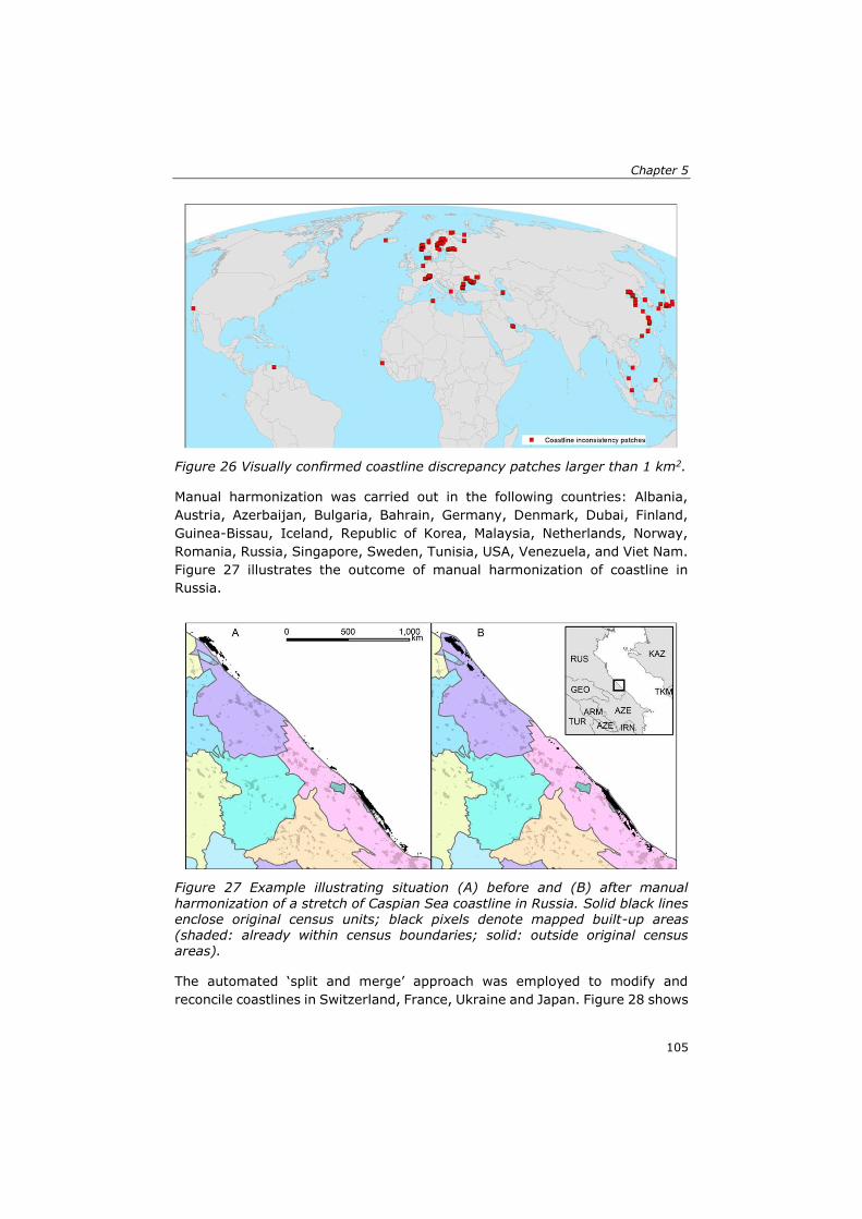
Chapter 5
105
Figure 26 Visually confirmed coastline discrepancy patches larger than 1 km2.
Manual harmonization was carried out in the following countries: Albania,
Austria, Azerbaijan, Bulgaria, Bahrain, Germany, Denmark, Dubai, Finland,
Guinea-Bissau, Iceland, Republic of Korea, Malaysia, Netherlands, Norway,
Romania, Russia, Singapore, Sweden, Tunisia, USA, Venezuela, and Viet Nam.
Figure 27 illustrates the outcome of manual harmonization of coastline in
Russia.
Figure 27 Example illustrating situation (A) before and (B) after manual
harmonization of a stretch of Caspian Sea coastline in Russia. Solid black lines enclose original census units; black pixels denote mapped built-up areas (shaded: already within census boundaries; solid: outside original census
areas).
The automated ‘split and merge’ approach was employed to modify and
reconcile coastlines in Switzerland, France, Ukraine and Japan. Figure 28 shows

Enhanced data and methods for improving open and free global population grids: putting
‘leaving no one behind’ into practice
106
the automated harmonization of coastlines applied along a stretch of Black Sea
coast in Ukraine.
Figure 28 Example of automated approach to mitigate inconsistencies along the coastline of Ukraine. This example shows the generation of a 2-km buffer that was split using the ‘split and merge’ approach. Solid black lines enclose original census units; solid blue line represents the extended boundary into the
sea through 2-km buffer; solid red lines represent the splitting of buffer into parts assigned to the nearest neighbouring unit; black pixels represent mapped built-up areas (shaded: already within census boundaries; solid: outside original census areas).
Although the detected anomalies may be significant for some applications such
as the present one, and relevant from the perspective of data consistency, not
all necessarily constitute errors in the original source data. Both in the case of
coastline deficiencies and for units declared as unpopulated, the discrepancies
may be due to anachronism between data sources. Coastal zones are typically
attractive and dynamic areas from a settlement perspective, and geospatial
data on administrative divisions used to support population estimates may not
reflect the current land extents and settlement expansion obtained by land
reclamation. Significant settlement expansion through land reclamation has
been taking place in Asia (especially in China) and in the Middle East and it is
important that time series of population grids capture and represent that
process. Also, settlements can extend over water bodies such as floating
settlements thus being located beyond the formal coastline. These can and are
captured by GHSL, as no land mask is imposed a priori to limit detection of
built-up. Instead of adopting the classical approach rooted in topography (e.g.
Anderson et al. 1976) of following a hierarchical top-down procedure in
abstracting the Earth surface into categories, GHSL adopts a people-centric
approach that departs from the detection of human presence, and only then
classifies phenomena into higher abstraction levels such as settlement classes
(Pesaresi and Ehrlich 2009) (for explanation of GHSL family of products and

Chapter 5
107
analysis see Melchiorri et al. 2018). This approach may be a better match for
the census paradigm, which aims to first identify where all people are so they
can be surveyed and characterized. In this capacity, perhaps GHSL mapping
of built-up could assist in planning census campaigns, especially in remote
areas of countries having dynamic population trends that have not conducted
a census in a long time.
Regarding the many discrepancies observed along coastlines, it is possible that
these originate in differences in scale and level of detail among datasets, and
at times can be introduced by the coarser detail of the database of Global
Administrative Areas (GADM 2011) when boundaries are adjusted to a global
framework in the GPW workflow.
Finally, it is important to note that the built-up structures detected and mapped
could include abandoned or seasonal settlements, or otherwise non-residential
facilities (e.g. ports, industrial areas). Ideally, a combination of census’ spatial
detail and attributes or ancillary data would allow further discrimination of land
use according to application needs. In practice, the two addressed anomalies
can be regarded as an expression of the same underlying issue, i.e. complete
omission of population counts (due to undercounting/under-reporting or poor
census geography) against contradicting evidence. It has been shown that a
similar approach can be used to automatically mitigate systematic issues of
both types.
5.4 Conclusions Global population distribution grids are increasingly required and relied upon
for many applications. These datasets are mostly produced by gridding or
disaggregating counts from official population census and estimates. Despite
the continuous advancements in population gridding methods, these usually
do not address ex-ante issues affecting input population statistics. Availability,
quality and detail of national data reporting on population is highly
heterogeneous, and the best available global geospatial census data is not
immune to shortcomings. These propagate to derived population distribution
grids and may negatively impact their applications, in an age of new
Development Agendas whose effective monitoring relies heavily on accurate
and reliable geospatial population data and calls for universal inclusiveness of
people. Exploring the improved capacities of recent global settlement data
derived from remote sensing, we have sought to improve the mapping of popu-
lation distribution by addressing some of these shortcomings.
New automated procedures to detect and mitigate major discrepancies and
anomalies occurring in geospatial census data were developed, tested and
implemented, while minimizing changes to the original data. Global and
consistent remote sensing-derived data reporting on built-up presence was
used to revise census units deemed as ‘unpopulated’ and to harmonize
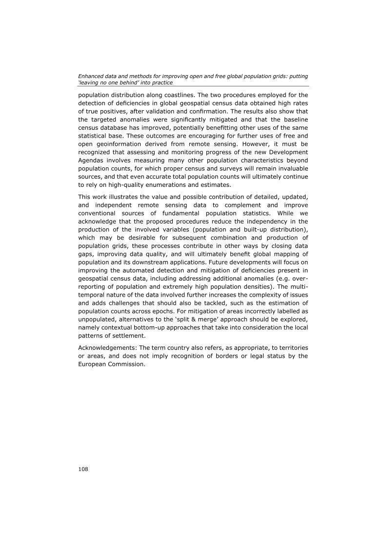
Enhanced data and methods for improving open and free global population grids: putting
‘leaving no one behind’ into practice
108
population distribution along coastlines. The two procedures employed for the
detection of deficiencies in global geospatial census data obtained high rates
of true positives, after validation and confirmation. The results also show that
the targeted anomalies were significantly mitigated and that the baseline
census database has improved, potentially benefitting other uses of the same
statistical base. These outcomes are encouraging for further uses of free and
open geoinformation derived from remote sensing. However, it must be
recognized that assessing and monitoring progress of the new Development
Agendas involves measuring many other population characteristics beyond
population counts, for which proper census and surveys will remain invaluable
sources, and that even accurate total population counts will ultimately continue
to rely on high-quality enumerations and estimates.
This work illustrates the value and possible contribution of detailed, updated,
and independent remote sensing data to complement and improve
conventional sources of fundamental population statistics. While we
acknowledge that the proposed procedures reduce the independency in the
production of the involved variables (population and built-up distribution),
which may be desirable for subsequent combination and production of
population grids, these processes contribute in other ways by closing data
gaps, improving data quality, and will ultimately benefit global mapping of
population and its downstream applications. Future developments will focus on
improving the automated detection and mitigation of deficiencies present in
geospatial census data, including addressing additional anomalies (e.g. over-
reporting of population and extremely high population densities). The multi-
temporal nature of the data involved further increases the complexity of issues
and adds challenges that should also be tackled, such as the estimation of
population counts across epochs. For mitigation of areas incorrectly labelled as
unpopulated, alternatives to the ‘split & merge’ approach should be explored,
namely contextual bottom-up approaches that take into consideration the local
patterns of settlement.
Acknowledgements: The term country also refers, as appropriate, to territories
or areas, and does not imply recognition of borders or legal status by the
European Commission.
109
Chapter 6. An Improved Global Analysis
of Population Distribution in Proximity
to Active Volcanoes38
38 This chapter is published as: Freire, S.; Florczyk, A.J.; Pesaresi, M.; Sliuzas, R., 2019. An improved global analysis of population distribution in proximity to active volcanoes, 1975–2015. ISPRS Int. J. Geo-Inf., 8(8), 341.

An improved global analysis of population distribution in proximity to active volcanoes
110
Abstract: Better and more detailed analyses of global human exposure to hazards and
associated disaster risk require improved geoinformation on population
distribution and densities. In particular, issues of temporal and spatial
resolution are important for determining the capacity for assessing changes in
these distributions. We combine the best-available global population grids with
latest data on volcanoes, to assess and characterize the worldwide distribution
of population from 1975–2015 in relation to recent volcanism. Both Holocene
volcanoes and those where there is evidence of significant eruptions are
considered. A comparative analysis is conducted for the volcanic hot spots of
Southeast Asia and Central America. Results indicate that more than 8% of the
world’s 2015 population lived within 100 km of a volcano with at least one
significant eruption, and more than 1 billion people (14.3%) lived within 100
km of a Holocene volcano, with human concentrations in this zone increasing
since 1975 above the global population growth rate. While overall spatial
patterns of population density have been relatively stable in time, their
variation with distance is not monotonic, with a higher concentration of people
between 10 and 20 km from volcanoes. We find that in last 40 years in
Southeast Asia the highest population growth rates have occurred in close
proximity to volcanoes (within 10 km), whereas in Central America these are
observed farther away (beyond 50 km), especially after 1990 and for Holocene
volcanoes.
6.1 Introduction Volcanic eruptions are among the most powerful and destructive natural
hazards on Earth, capable of causing widespread human suffering and
extensive economic losses, both from direct impacts and through the
disturbances to livelihoods arising from indirect or cascading effects (e.g., via
disruptions of air transport, through originating tsunamis, etc. (UNISDR
2015b). Severe eruptions can cause rapid global changes by modifying weather
patterns, disrupting climate, and, as in the past, induce mass extinctions of
species (National Academy of Sciences, 2017). Although moderate to large
volcanic eruptions are infrequent, these are potentially high-consequence
incidents, especially for nearby populations due to lava flows, ash deposition,
pyroclastic events, and other phenomena (Dilley et al. 2005). Still, the 2010
eruption of Eyjafjallajökull volcano in Iceland demonstrated that even modest
eruptions in relatively remote locations can have global impacts (National
Academy of Sciences, 2017, Ragona et al. 2011). Volcanic activity can have a
disproportionate effect on livelihoods and economy because of high systemic
vulnerability (Poljanšek et al. 2017).
Volcanoes located in densely populated areas, however, do not need to have
powerful eruptions to produce devastating effects. In such settings, even
small-to moderate-sized eruptions may constitute severe threats, by

Chapter 6
111
generating multiple hazards which can affect areas from the immediate vicinity
up to hundreds of kilometres distance (for detailed discussion see Chester et
al. 2000, Brown et al. 2017). In a study of past disasters, residents make up
the largest number of fatalities (Brown et al., 2017).
Beyond their destructive power, volcanoes and volcanic activity can also
benefit humans and their livelihoods. Among their major beneficial effects are
the provision of nutrients to the surrounding soil, favoring agricultural
productivity—an important aspect in agrarian societies—but also economic
activities such as resource extraction (e.g., Sulfur mining), tourism, and
geothermal energy (National Academy of Sciences, 2017). Such benefits help
to explain population concentrations in their vicinity. In addition, tropical
volcanoes provide climatic advantages relative to surrounding regions (Small
et al., 2001), which may have promoted human settlement and the clustering
of people. Such clustering in proximity to active volcanoes creates exposure
levels with changes that vary in space or time (Strader et al., 2015). This
exposure combines with existing vulnerabilities to generate risk and the
potential for losses. Evidence indicates that exposure of persons and assets in
all countries has increased faster than vulnerability has decreased, thus
generating new risks (UNISDR, 2015).
Evaluating potential or actual human exposure for global disaster risk
assessment is as essential as it is challenging, being limited by the availability
and quality of geophysical and socio-economic data (Lerner-Lam, 2007,
Peduzzi et al. 2009a). As a result, previous estimations of human exposure
were typically conducted for small areas and without a temporal dimension, or
merely approximated with coarse population geoinformation (~1 km grids).
However, the rapid increase in exposure of population and assets is currently
a major driver of growing disaster risk (UNISDR, 2013), requiring adequate
global geoinformation layers depicting the distribution and densities of
population. Such geoinformation is valuable throughout the emergency
management cycle, but for timely and efficient response it should be prepared
and made available beforehand (Freire, 2010). After a disaster event, the
quality and granularity of population data have a direct effect on response and
lives saved (National Research Council, 2007). Although global population grids
have been produced since the 1990s, they have suffered from some issues
which limit their usability (Linard et al. 2012, Mondal et al. 2012). Among these
are their coarse spatial resolution, incomplete discrimination of settlements
(especially smaller ones), and the use of dichotomous maps of built-up in their
construction. Also, for change detection and analysis, a coherent and robust
spatio-temporal production model is required to allow objective comparisons.
Concerning volcanic risk, Andredakis et al. 2015 highlight that risk elements
are on the rise, most notably population exposure. The shifting focus of
urbanization from developed to developing countries taking place in recent
decades is also increasing global exposure to natural hazards, including

An improved global analysis of population distribution in proximity to active volcanoes
112
volcanism (Chester et al. 2000). Volcanic activity remains a constant threat
globally and the number of people at risk from volcanism is rising with
increased urbanization and population growth (National Academies of Sciences
2017, Chester et al. 2000, Brown, et al. 2017, Ewert 2004). However, volcanic
risk analysis and assessment at the global scale is not as advanced as for other
hazards such as flooding, earthquakes and tropical cyclones (Poljanšek et al.
2017), being limited by the availability and quality of data (Pan et al. 2015),
especially regarding their consistency and detail. Similarly to earthquakes,
volcanic eruptions are difficult to mitigate technologically (Riede, 2016), in that
the hazard component can hardly be decreased by human action. While
expected losses may be lower than those from other hazards at a global scale,
in affected regions, they can be very significant. Since 1950, an average of 31
volcanoes have erupted each year (United Nations, 2015), and at any one time
at least 20 are erupting (Siebert et al. 2010, Siebert et al. 2015). Given this
context, major gains to disaster risk reduction are to be obtained through
reductions in vulnerabilities and especially in exposure, requiring improved
assessments of these components.
6.1.1 Potential Global Population Exposure to Volcanic Hazard —Narrowing Data Gaps
Several assessments of potential worldwide population exposure to volcanic
hazard have been conducted using globally-available population grids, e.g.,
(Dilley et al. 2005, Small and Naumann 2001, Aspinall et al. 2011, Brown et
al. 2015). However, most such studies are now relatively outdated, or use
coarse population geoinformation. Often, assessments are based on data that
are neither open nor free. Small and Naumann (Small and Naumann 2001) in
their landmark work quantified human proximity to both Holocene and
historically active volcanoes for 1990, but underlined that the spatial resolution
of population data used (GPWv2) imposes limitations on the analysis and is not
adequate for detailed assessment of potential volcanic risk. Ewert and Harpel
(Ewert et al. 2004) have proposed a Volcano Population Index (VPI) to make
objective estimates and comparisons of the number of people at risk from
volcanic hazards. Within a given radius of a volcanic vent, the index quantifies
one component of risk—population—from one volcano to another. The authors
have noted that the 1-kilometer grid size of the population grid used
(LandScan) was the principal limiting factor in making precise estimates of
population at risk (Ewert et al. 2004). The Population Exposure Index (PEI)
(Aspinall et al. 2011) is one of the prominent indices used in assessing volcano
risk. It is based on the population within 10, 30, and 100 km of a volcano,
which is then weighted according to evidence on historical distributions of
fatalities within a given distance from volcanoes. The PEI is divided into seven
levels, from sparsely to very densely populated areas. The authors have stated
that the main drawback of such methods is that they rely on a number of
parameters having high uncertainty or that are simply unknown for many

Chapter 6
113
volcanoes. This limits application of the method mainly to those with good
historical records (Scandone et al. 2016). As a simpler and more direct way to
compare different volcanoes or volcanic areas, (Scandone et al. 2016) have
proposed a volcanic risk coefficient (VRC) using the number of people that may
be affected by the maximum expected eruption as a main variable. In addition
to the estimation of this specific hazard information, this still requires detailed
and comparable population distribution data.
Common to all these efforts is the need for up-to-date and spatially-explicit
population distribution data, which are globally-consistent and have sufficient
resolution to support detailed analyses and comparisons. This is especially
important as databases of locations and features of potential volcano hazard
(i.e., GPV) are also subject to frequent revisions and updates, thereby inviting
parallel re-assessments of global and regional potential population exposure.
Improved modeling and mapping of global population distribution can be
achieved with remote sensing imagery and methods, which have been evolving
towards a more detailed, objective and independent data source on the human
presence on the Earth surface (Freire et al. 2018a). The multiscale synoptic
perspective is considered one of the core strengths of remote sensing when it
comes to questions of urban and socio-economic development and in regards
to the closely interlinked disaster risk domain (Aubrecht et al. 2017b). In the
specific case of population exposure to volcanic hazard, (Brown et al. 2017)
point out that “moderate resolution satellite imagery, such as that provided by
the Landsat series, could provide more spatially explicit quantifications of
settlement patterns in the vicinity of potentially active volcanoes. More
recently, (Pittore et al. 2017) advocate for full exploitation of rapid, large-scale
data collection based on remote sensing, while also stressing that
dissemination of exposure data is key to empowering end-users and
communities and for allowing and encouraging risk evaluation.
6.1.2 The Contribution of the Global Human Settlement Layer (GHSL) to DRM
The recent application of new cost-effective, automated and fully replicable
data classification methods (e.g., symbolic machine learning) to contemporary
open and free global satellite imagery collections have enabled the emergence
of a new generation of geospatial data derived from remote sensing, led by the
Global Human Settlement Layer (GHSL) (Pesaresi and Ehrlich 2009). These
developments allowed the global mapping of built-up areas and settlements
with unprecedented spatio-temporal detail and accuracy (Pesaresi et al. 2009,
Pesaresi et al. 2013, Pesaresi et al. 2016), under a set of pragmatic
requirements and principles summarized in (Melchiorri et al. 2019). Among
other uses, these new datasets are providing an effective contribution to
population disaggregation and other population distribution modeling efforts,
especially due to a combination of:

An improved global analysis of population distribution in proximity to active volcanoes
114
Semantic robustness and interoperability
Currency of data
Spatial detail
Global coverage
Temporal depth
Provision of open and free data
GHSL’s enhanced spatio-temporal mapping of buildings and density of built-up
areas offers a suitable proxy for the location of people and, as such, is being
used to improve the disaggregation of census data into derived population
grids (Freire et al. 2015d, Freire et al. 2016a, Linard et al. 2017, Nieves et al.
2017, Balk et al. 2019).
From its inception, development of GHSL was driven by requirements for post-
disaster and post-conflict damage, needs and reconstruction assessment,
including refugee camps and temporary, rapidly-changing human settlement
monitoring (Pesaresi et al. 2015c). Therefore Disaster Risk Management and
Reduction is a major field of application of GHSL data, and among the uses of
its population distribution grids (GHS-POP) are the baseline estimation of
multi-temporal exposure to global hazards (Pesaresi et al. 2017, Ehrlich et al.
2018b) and assessment of impacts from climate hazards (Ehrlich et al. 2018a),
including the current and future projections of risk of river flood (Alfieri et al.
2017) (https://www.efas.eu; http://www.globalfloods.eu), and support to
creation of risk indices for management for humanitarian crises and disasters
(e.g., INFORM—Index for Risk Management (http://www.inform-index.org).
The GHSL layers and especially population distribution data enable conducting
more updated, refined, and longitudinal assessments of population potentially
affected by different types of natural hazards (Ehrlich et al. 2018b), including
threats posed by volcanoes (Freire et al. 2016b). Due to their characteristics,
it is expected that these new population data can further advance, update, and
detail assessment of population distribution in the vicinity of active volcanoes
and contribute to enhance estimations of potential exposure to this type of
hazard.
In this article, we aim to characterize with unprecedented detail the changes
in the distribution of human population in proximity to historically active
volcanoes, focusing on the last 40 years. We do that by combining detailed
geospatial grids of global population densities for the 1975–1990–2000–2015
period with the latest data on distribution of volcanoes on Earth, considering
both Holocene volcanoes and those having significant eruptions. We
investigate the recent evolution and current distribution of population in
relation to historical volcanism and discuss how overall potential population
exposure and density patterns have been varying with distance. More detailed
attention is dedicated to Southeast Asia and Central America, where
concentrations of people in vicinity of volcanoes are greater than in other
Chapter 6
115
volcanic regions. This work details and updates preliminary research done by
Freire et al. 2016b and shows the value of using the more recent datasets in
future assessments of volcanic risk.
6.2 Materials and Methods In Section 6.2.1., we present and discuss the datasets used, including a
description of the production and features of the global population grids that
made this study possible, and the global datasets of volcanoes. In Section 6.2.2
we present the methodology that was applied for assessing global population
distribution in relation to historical and significant volcanism.
6.2.1 Data
6.2.1.1 Global Population Distribution Grids 1975–2015
In order to assess population distribution in relation to distance to volcanoes,
we have used population grids for 1975, 1990, 2000, and 2015 produced in
the frame of the Global Human Settlement Layer (GHSL) project. These grids
(GHS-POP), reporting the distribution and density of total resident population
per 250-m cell, are created by using maps of density of built-up areas (Pesaresi
et al. 2016) for matching epochs as proxy for disaggregating best-available
population estimates (Freire et al. 2016a).
GHS-POP is based on population estimates provided by CIESIN’s Gridded
Population of the World (GPW) v4.10 for matching periods (CIESIN, 2016),
with national figures adjusted to UN World Population Prospects (Doxsey-
Whitfield, 2015). CIESIN collects and integrates the most recent and finest
resolution census data available, and the CIESIN-GPWv4.10 input dataset
includes the latest round of censuses (2010–2011) and comprises more than
12 million census or administrative units, with average spatial resolution
varying widely by country.
The GHS-POP population grids effectively harmonize and increase the
resolution of this variable in space and time by using consistent ancillary data
and methods. Among the specific methodological features of these grids are:
(i) the use of a single spatially and temporally-explicit proxy (built-up
areas from GHSL);
(ii) this proxy is mostly of higher spatial resolution than census data and
is derived with a consistent approach;
(iii) the employment of a simple, transparent and consistent methodology
for population disaggregation.
GHS-POP is also unique among current global population grids in that cell
values represent both counts and densities of population, by using as native
projection the World Mollweide equal-area projection. The latest release of
GHS-POP used in this study (made publicly available in 2019), mitigates

An improved global analysis of population distribution in proximity to active volcanoes
116
important shortcomings of previous population grids by improving
representation of distributions along coastlines and critically revising areas
declared as ‘unpopulated’ but where significant evidence of human habitation
existed (Freire et al. 2018a). Therefore GHS-POP is especially suited for
supporting Disaster Risk Management (DRM) tasks by refining distribution of
resident population to known places of human shelter and activities (i.e.,
buildings), where most people spend the majority of their time. Due to these
characteristics and given that GHS-POP is currently the only global dataset that
spans the last 40 years with comparable, detailed, open, and free data on
distribution of population in settlements, it allows investigating population
distribution in proximity to volcanoes in this period.
6.2.1.2 Global Geographical Distribution of Volcanoes
The proximal analysis of population was conducted considering two widely used
global datasets of volcanoes, available online: the Holocene Volcano List v.
4.7.6 (Volcanoes of the World 4.7.6.) of the Smithsonian Institution’s Global
Volcanism Program (GVP) (Global Volcanism Program, 2013) and the NOAA
Significant Volcanic Eruption Database (NOAA, 2019), this one also based on
GVP.
The Holocene Volcano List (HV in this article) is a global listing of volcanoes
believed to have been active during the Holocene period (the last ~10,000
years). This database includes information on the latitude, longitude, elevation,
type of volcano, and last known eruption. The HV database is frequently
updated and v. 4.7.6 used in this work includes 1432 volcanoes, of which 118
are submarine volcanoes and 83 correspond to volcanic fields.
The Significant Volcanic Eruption Database (SV in this article) is a global listing
of over 500 significant eruptions. The current version used here lists 826
eruptions for 265 volcanoes. This database includes information on volcanoes
(i.e., latitude, longitude, geographic location, elevation, type of volcano), their
eruptions (date of eruption, the assigned Volcanic Explosivity Index (VEI) and
associated events, such as tsunami and/or earthquake), and impact (fatalities,
estimated economical damage, etc.). A significant eruption is defined as one
that meets at least one of the following criteria: caused fatalities, produced
moderate damage (approximately 1 million USD or more), had a Volcanic
Explosivity Index (VEI) of 6 or larger, caused a tsunami, or was associated with
a major earthquake (NOAA, 2019). Figure 29 shows the global distribution of
volcanoes from the above databases that were considered in this study.

Chapter 6
117
Figure 29 Distribution of the two global datasets of volcanoes used in this study: Holocene Volcano List v4.7.6 (HV) and Significant Volcanic Eruption
Database (SV) (World Mollweide projection).
6.2.2 Assessing Global Population Distribution and Volcanism
We analyzed global population distribution as a function of distance to
volcanoes in 1975, 1990, 2000, and 2015, using the 250 m population grids
(GHS-POP) for the respective epochs. Using GIS software, population
distribution was analyzed up to a radial distance of 100 km from volcanoes, by
buffering each volcano in 1 km steps and conducting zonal analysis of
population grids. Given the global scope of this analysis and the challenges
involved with measuring accurately both distances and areas (impossible in
same cartographic projection), and the fact that population grids are produced
in equal-area projection (thus representing both counts and densities), we
devised the following procedure:
(1) Calculation of distance buffers from volcanoes in World Equidistant
Cylindrical projection;
(2) Merging the resulting buffers by distance (i.e., dissolve by distance
function);
(3) Re-projection of the distance buffers to World Mollweide projection;
(4) Rasterization to the working grid (i.e., 250 m World Mollweide aligned
with the GHS global grid), and calculation of landmass surface and
population counts per each buffer in World Mollweide.
This approach tries to minimize distortions in distances, areas, and population
counts. The considerable effort expended to maintain the accuracy of
underlying databases is an aspect that is absent (or omitted) from previous
global analyses (Dilley et al. 2005, Small and Naumann 2001, Aspinall et al.

An improved global analysis of population distribution in proximity to active volcanoes
118
2011, Brown et al. 2015), therefore constituting a relevant new feature of the
current analysis.
For discussing the results, four distances from volcanoes were selected as
being especially relevant: 10, 30, 50, and 100 km. Aspinall et al. (2011)
adopted 10 and 30 km in their PEI proposal. Moreover, 10 km is a frequently
used distance for evacuation after moderate to large eruptions. Regarding the
50 km mark, (Brown et al. 2017) have identified that close to 100% of volcanic
fatalities registered have occurred within this distance from volcanoes. 100 km
is considered relevant as a maximum distance from volcanoes for assessing
the direct effects of volcanic eruptions, since lethal pyroclastic flows and surges
(Nakada, 2000), and lahars (Rodolfo, 2000) may occasionally extend to these
distances. Among twelve destructive phenomena associated with volcanic
eruptions, it is estimated that seven can potentially reach such a distance
(Chester et al. 2000). Given the observation by (Small and Naumann 2001)
that higher population densities in Southeast Asia and Central America lie in
closer proximity to volcanoes than in other volcanic regions, we conduct a more
detailed analysis of results for these regions. As in that work, volcanic regions
are considered to be those with a significant number of persistently active
volcanoes.
6.3 Results and Discussion
6.3.1 Global Population Distribution from 1975 to 2015 in Relation to Volcanism
This section presents and discusses the global distribution of population from
1975 to 2015 in relation to volcanism, considering both overall population in
each period and annual growth rates by distance to both HV and SV. While the
first part focuses on significant distance ranges up to 100 km of volcanoes, a
second part analyses the specific spatio-temporal patterns of population
density within 50 km of volcanoes in more detail.
Table 16 shows total accumulated population within selected distance ranges
(radial distances) from Holocene volcanoes (HV), for each period considered.
Results show that the total population living in proximity of Holocene volcanoes
(HV) is very significant and that this amount has been increasing steadily in
last 40 years. In 2015, more than 1 billion people, 14.3% of the global
population, are estimated to live within a range of potential direct impact of
volcanic eruptions (i.e., within 100 km). Close to 60 million people are
estimated to live within potential evacuation range worldwide (i.e., within 10
km).

Chapter 6
119
Table 16 Population (in millions and as percentage of World total) by radial distance from Holocene volcanoes (HV) in 1975, 1990, 2000, and 2015.
1975 1990 2000 2015
Dist. (km)
Pop. [106]
% Pop. [106]
% Pop. [106]
% Pop. [106]
%
10 29 0.7 41 0.8 49 0.8 59 0.8 30 176 4.3 243 4.6 284 4.6 340 4.6 50 301 7.4 415 7.8 489 8 592 8.1 100 566 13.9 751 14.1 870 14.2 1054 14.3
Global 4,061 100 5,310 100 6,127 100 7,349 100
Concerning population growth rates in vicinity of Holocene volcanoes (HV)
(Table 17), these are generally decreasing with time, accompanying global
population trends. These rates were especially high from 1975 to 2000, and
were increasing with proximity to HV. However, despite slowing down with
time, rates in vicinity of HV were largely above the global average in all periods.
Table 17 Compound annual growth rate of population by radial distance from Holocene volcanoes (HV) for each time interval.
Distance (km)
1975–1990
1990–2000
2000–2015
1975–2015
10 2.29 1.76 1.27 1.78
30 2.19 1.58 1.19 1.66 50 2.17 1.64 1.29 1.71 100 1.90 1.48 1.29 1.57
Global 1.80 1.44 1.22 1.49
Table 18 and Table 19 refer to variation of population within selected distances
of volcanoes with significant eruptions (SV). Results show that this population
has also been increasing steadily and amounts to 616 million in 2015, or 8.4%
of global population. Also very significant are the 21 million people living within
10 km of these volcanoes.
Table 18 Population (in millions and percentage of World total) by radial
distance from volcanoes with significant eruptions (SV) in 1975, 1990, 2000, and 2015.
1975 1990 2000 2015
Distance (km)
Pop. [106]
% Pop. [106]
% Pop. [106]
% Pop. [106]
%
10 12 0.3 16 0.3 18 0.3 21 0.3 30 87 2.2 115 2.2 130 2.1 150 2 50 169 4.1 222 4.2 254 4.1 297 4 100 333 8.2 444 8.4 515 8.4 616 8.4
Global 4,061 100 5,310 100 6,127 100 7,349 100
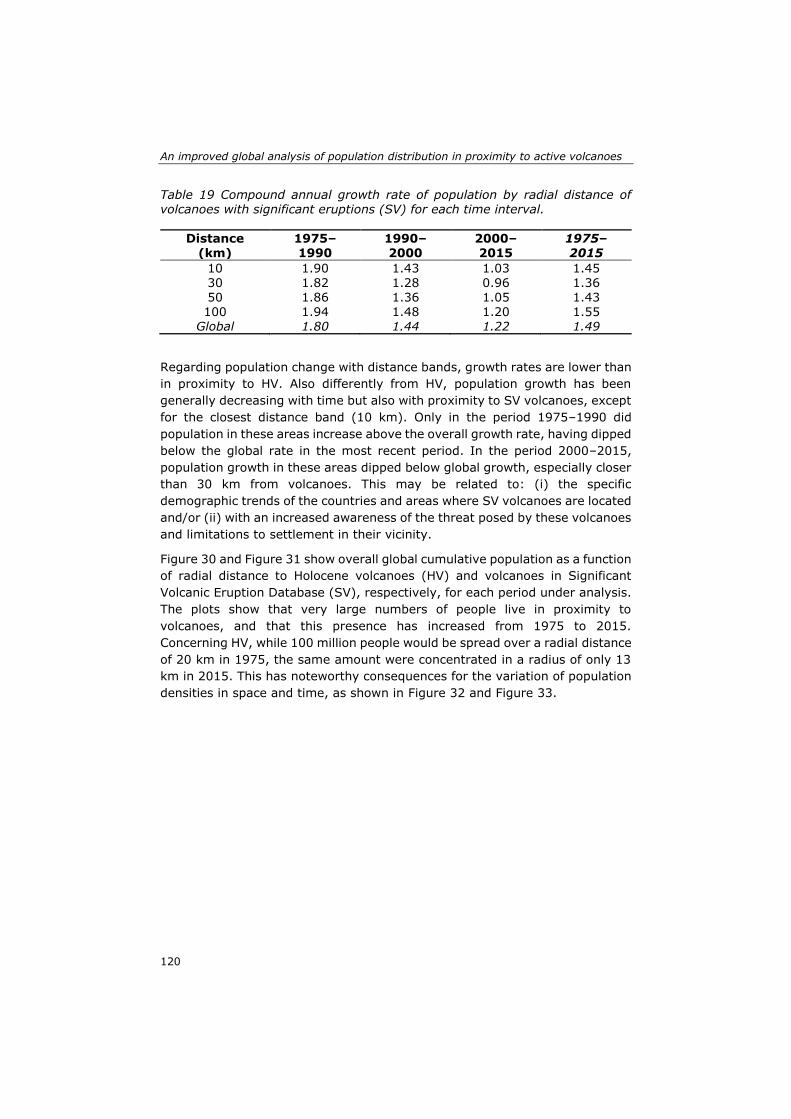
An improved global analysis of population distribution in proximity to active volcanoes
120
Table 19 Compound annual growth rate of population by radial distance of volcanoes with significant eruptions (SV) for each time interval.
Distance (km)
1975–1990
1990–2000
2000–2015
1975–2015
10 1.90 1.43 1.03 1.45 30 1.82 1.28 0.96 1.36 50 1.86 1.36 1.05 1.43 100 1.94 1.48 1.20 1.55
Global 1.80 1.44 1.22 1.49
Regarding population change with distance bands, growth rates are lower than
in proximity to HV. Also differently from HV, population growth has been
generally decreasing with time but also with proximity to SV volcanoes, except
for the closest distance band (10 km). Only in the period 1975–1990 did
population in these areas increase above the overall growth rate, having dipped
below the global rate in the most recent period. In the period 2000–2015,
population growth in these areas dipped below global growth, especially closer
than 30 km from volcanoes. This may be related to: (i) the specific
demographic trends of the countries and areas where SV volcanoes are located
and/or (ii) with an increased awareness of the threat posed by these volcanoes
and limitations to settlement in their vicinity.
Figure 30 and Figure 31 show overall global cumulative population as a function
of radial distance to Holocene volcanoes (HV) and volcanoes in Significant
Volcanic Eruption Database (SV), respectively, for each period under analysis.
The plots show that very large numbers of people live in proximity to
volcanoes, and that this presence has increased from 1975 to 2015.
Concerning HV, while 100 million people would be spread over a radial distance
of 20 km in 1975, the same amount were concentrated in a radius of only 13
km in 2015. This has noteworthy consequences for the variation of population
densities in space and time, as shown in Figure 32 and Figure 33.

Chapter 6
121
Figure 30 Cumulative population as a function of radial distance to Holocene volcanoes (HV), in 1975, 1990, 2000, and 2015.
Figure 31 Cumulative population as a function of radial distance to volcanoes in Significant Volcanic Eruption Database (SV), in 1975, 1990, 2000, and 2015.

An improved global analysis of population distribution in proximity to active volcanoes
122
Figure 32 Average population density as a function of radial distance to Holocene volcanoes (HV), in 1975, 1990, 2000, and 2015.
Figure 33 Average population density as a function of radial distance to volcanoes in Significant Volcanic Eruption Database (SV), in 1975, 1990, 2000, and 2015.
Differently from some previous analyses (e.g., Small and Naumann 2001), we
have considered all volcanoes listed in the databases regardless of their type
or location, as e.g., submarine volcanoes may still affect populations on land
upon erupting, as many are located in proximity to inhabited areas. This is
especially relevant for remote archipelagos (such as Tonga, French Polynesia,

Chapter 6
123
Solomon Islands Guam, Hawaii, Mariana Islands), where potential exposure
and risk is typically overlooked in global analyses and where DRM poses specific
challenges. In fact, we think this may be a ‘hidden’ source of potential exposure
and risk that should deserve more attention in future research. Of 118
submarine volcanoes in the HV list, 76 have documented eruptions.
Figure 32 and Figure 33 show the average population densities (over land) by
radial distance to volcanoes. These charts show that relatively high population
densities occur in the vicinity of all volcanoes, especially of those with
significant eruptions (above the overall global densities over land, which are
27 and 49 people/km2 in 1975 and 2015, respectively); and these densities
increase sharply away from volcanoes but in very close proximity, especially
from SV, in whose vicinity densities are significantly higher. Moreover, while
maintaining the overall pattern, those densities have been increasing
considerably since 1975, particularly in the period 1975–1990. However, it is
at a distance of 10 to 20 km from Holocene volcanoes that the absolute
increase in population density has been greatest (additional 75 persons/km2),
from 1975 to 2015.
In all periods, population density generally increases with close proximity to
volcanoes, peaking at around 15–20 km away, and then decreases sharply in
their immediate vicinity, but still maintaining relatively high densities. This
sharp decrease may be due to presence of steep slopes, volcanic activity, or
enforcing of exclusion zones for settlement. This pattern is even more striking
for volcanoes with significant eruptions (SV), where overall population
densities are higher (up to 270 people/km2), with obvious implications for
exposure, risk analyses, and potential impacts. This pattern is dissimilar from
the monotonically decreasing densities reported by Small and Naumann 2001.
This difference may be the outcome of sharper analyses enabled by the
characteristics of the new population grids, i.e., effective disaggregation to
built-up areas and higher spatial detail.
These results further detail, revise and update previous estimates, such as that
of UNISDR 2015b that states “... at present, more than 800 million people in
86 countries live within 100 km of a volcano that could potentially erupt (GVM,
2014a)”, and that “... over 29 million people worldwide live within just 10 km
of active volcanoes, and around 800 million people live within 100 km” (Brown
et al. 2015). Likely reasons for such disagreement include their reliance on
conceptually different population grids (e.g., LandScan versus GHS-POP), and
their reliance on older census data. Also, LandScan does not depart from or
aim to model distribution of residential population, from which population living
in proximity can be estimated with more confidence, but instead maps ambient
population.

An improved global analysis of population distribution in proximity to active volcanoes
124
6.3.1.1 Sources of Uncertainty
As with all global data, both the volcano datasets and the population grids are
affected by error and uncertainty. This analysis is performed using a 250 m
population grid, which also makes it sensitive to uncertainty in spatial
precision. The uncertainties in GHS-POP mostly result from the quality and
reliability of censuses and the capacity to fully detect built-up in diverse
landscapes using heterogeneous Landsat image archives (Pesaresi et al.
2016). Such issues typically worsen with temporal distance from the current
period (for a more detailed discussion, see reference (Freire et al. 2018a).
Despite the mitigation procedures implemented in the production of the current
population grids, some issues remain unsolved in global population data, which
should not be used for pixel level assessments.
Issues of spatial accuracy and precision also affect the GVP datasets in which
volcanoes are represented through points (coordinate pairs), and a single point
frequently refers to a group of volcanoes or craters (e.g., volcanic fields) or
giant calderas (e.g., Yellowstone, USA); for some of these, due to their size
and extent, an areal feature (polygon) would be a better representation for the
potential hazard source. Also, the geographical coordinates (decimal degrees)
are often coarse with precision sometimes limited to the first decimal, which
corresponds to a real world precision of about 5.5 km. This is clearly insufficient
for detailed analyses in close proximity to volcanoes. This vagueness and low
spatial precision reduce accuracy and discourage more detailed analyses.
These and other uncertainties introduce limitations for studies: while these are
usually mitigated when aggregated assessments such as this one are
conducted, they can become apparent when analyses are carried out for
individual volcanoes or at very fine scale (e.g., very close proximity).
6.3.2 Population Distribution from 1975 to 2015 in Relation to Volcanism, in Southeast Asia and Central America
This section analyzes in more detail results for two important volcanic regions,
Southeast Asia and Central America. The first region comprises the countries
of Indonesia, Philippines, and East Timor, while the second includes Mexico,
Guatemala, Belize, Honduras, El Salvador, Nicaragua, Costa Rica, and Panama.
Figure 34 shows location of Holocene volcanoes in these regions and the
selected distances under analysis. SE Asia and Central America together
represent 40% of the total global population living within 100 km of volcanoes,
but with different contributions and patterns of population by radial distances
(Table 20).

Chapter 6
125
Figure 34 Selected distances from Holocene volcanoes in (A) Southeast Asia and (B) Central America.
Table 20 Population (in millions and percentage of region total) by radial distance of Holocene volcanoes (HV) and volcanoes in Significant Volcanic

An improved global analysis of population distribution in proximity to active volcanoes
126
Eruption Database (SV) in 1975, 1990, 2000, 2015, in Southeast Asia and Central America.
1975 1990 2000 2015
Dist. (km)
HV SV HV SV HV SV HV SV
Southeast Asia
10 11
(6.6%)
[4 (2.5%)
]
18 (7.3%
)
[7 (2.8%)
]
22 (7.5%
)
[8 (2.9%)
]
27 (7.4%
)
[10 (2.9%)
]
30 73
(42.5%)
[42 (24.2%
)]
109 (44.6%)
[59 (24.3%
)]
129 (44.3%)
[69 (23.7%
)]
153 (42.5%)
[81 (22.4%
)]
50 118
(68.4%)
[80 (46.2%
)]
171 (69.9%)
[113 (46.1%
)]
202 (69.6%)
[132 (45.4%
)]
243 (67.7%)
[157 (43.6%
)]
100 143
(82.8%)
[132 (76.2%
)]
207 (84.9%)
[189 (77.4%
)]
247 (85.1%)
[225 (77.4%
)]
301 (83.7%)
[272 (75.8%
)] Region
173 (100%) 244 (100%) 290 (100%) 359 (100%)
Central America
10 6
(7.1%)
[2 (3%)]
8 (6.9%
)
[3 (2.7%)
]
9 (6.8%
)
[3 (2.5%)
]
11 (6.4%
)
[4 (2.3%)
]
30 29
(35.3%)
[11 (14.1%
)]
40 (34.6%)
[16 (13.9%
)]
47 (34.1%)
[19 (13.8%
)]
57 (32.8%)
[23 (13.4%
)]
50 41
(50.3%)
[22 (27%)]
56 (49.1%)
[30 (26.4%
)]
67 (48.3%)
[36 (25.9%
)]
81 (46.7%)
[43 (24.9%
)]
100 57
(70.6%)
[44 (53.9%
)]
81 (70.3%)
[60 (52.2%
)]
97 (70%)
[71 (51.2%
)]
120 (69.4%)
[86 (49.7%
)] Region
81 (100%) 115 (100%) 139 (100%) 173 (100%)
In SE Asia the population within 100 km of HV has increased from 143 million
in 1975 to 301 million in 2015, representing 84% of the region’s inhabitants.
In Central America the population within this distance increased from 57 million
in 1975 to 120 million in 2015, comprising 69% of the region’s inhabitants.
Especially striking in SE Asia are the 10 and the 27 million people currently
living within 10 km of SV and HV, respectively, accounting for almost half of
the global population within this range of recently active volcanoes. This short
distance is especially problematic in small inhabited islands which are
completely contained within this range, where fast evacuation can be
particularly challenging.
However, while in SE Asia the share of total population within 100 km of HV
has increased (albeit slightly) between 1975 and 2000, in Central America this
value has been decreasing, and even more so when SVs are considered.

Chapter 6
127
Concerning the annual growth rates of population by radial distance of HV and
SV, Table 21 shows important differences between and within these regions.
Table 21 Compound annual growth rate of population by radial distance of Holocene volcanoes (HV) and volcanoes in the Significant Volcanic Eruption Database (SV), for each time interval, in Southeast Asia and Central America.
1975–1990 1990–2000 2000–2015 1975–2015
Dist. (km) HV SV HV SV HV SV HV SV
Southeast Asia 10 3.05 [3.15] 2.10 [2.16] 1.36 [1.34] 2.17 [2.22] 30 2.66 [2.37] 1.69 [1.49] 1.15 [1.05] 1.85 [1.65] 50 2.48 [2.32] 1.71 [1.59] 1.25 [1.15] 1.82 [1.7] 100 2.51 [2.44] 1.77 [1.74] 1.32 [1.29] 1.88 [1.83]
Region 2.34 1.75 1.43 1.85
Central America 10 2.14 [1.67] 1.67 [1.31] 1.07 [0.84] 1.62 [1.27] 30 2.21 [2.25] 1.75 [1.84] 1.21 [1.28] 1.72 [1.78] 50 2.19 [2.19] 1.74 [1.74] 1.24 [1.19] 1.72 [1.7] 100 2.31 [2.13] 1.88 [1.71] 1.41 [1.27] 1.86 [1.7]
Region 2.34 1.91 1.47 1.91
While in SE Asia the highest growth rates have occurred in close proximity to
HV and SV volcanoes (within 10 km), in Central America the strongest rates
are observed farther away (beyond 50 km), especially after 1990 and for HV.
Also, whereas in SE Asia much of this growth has occurred at rates well above
the regional ones between 1975 and 2000 (especially for HV), in Central
America increases stayed below regional rates for all distances and periods,
suggesting that areas more distant from volcanoes were favored for
settlement. While explaining the observed variations is beyond the scope of
this paper, we can offer some hypotheses for the underlying causes:
(a) Pressure for space in a context of relatively weak planning, causing
settlement to encroach on volcanoes (overall average population
densities are much higher in SE Asia than in Central America);
(b) More recent dates of eruptions and variations in risk perception.
Additional research is needed to test these and other hypotheses that may
explain settlement patterns.
Regarding variation of population densities in these regions in proximity of HV
and SV, Figure 35 and Figure 36 show some differences. For both volcano sets,
population densities are generally higher in SE Asia, especially in 2015 where
these can be more than twice those in Central America (HV). In SE Asia,
population densities increase faster with distance from HV and remain
relatively high (>400 persons/km2) up to 44 km away. Beyond 4 km, density
surpasses the overall mean for the region (78 and 163 persons/km2 in 1975
and 2015, respectively). There is a pronounced peak in densities around a
distance of 18–22 km that has intensified since 1975. Because this is

An improved global analysis of population distribution in proximity to active volcanoes
128
essentially a mountainous landscape, this may also reflect the average distance
of valley floors (or the mid-distance between consecutive mountains), where
conditions for settlement are more favorable. Figure 37 illustrates the situation
in 2015 in the Island of Java (Indonesia), showing the locations of Holocene
volcanoes, main cities, and the population distribution.

Chapter 6
129
Figure 35 Average population density in Southeast Asia (SEAsia) and Central America (CAm) as a function of radial distance of Holocene Volcanoes (HV), in 1975 and 2015.
Figure 36 Average population density in Southeast Asia (SEAsia) and Central
America (CAm) as a function of radial distance of volcanoes in Significant Volcanic Eruption Database (SV), in 1975 and 2015.

An improved global analysis of population distribution in proximity to active volcanoes
130
Figure 37 Island of Java (Indonesia), showing selected distances from Holocene volcanoes, main cities, and population distribution in 2015 from GHS-POP (World Mollweide projection).
Regarding SV volcanoes (Figure 36), in Central America densities increase
dramatically up to 6–8 km and remain high up to 16 km, decreasing markedly
after that distance. SE Asia displays a similar proximal pattern for both HV and
SV, with very high densities observed around 20 km from SV (700 people/km2)
and remaining high until 50 km away. These results suggest that the overall
settlement patterns observed, although specific for each region, were mostly
defined prior to 1975, especially in Central America. These spatio-temporal
patterns of settlement have consequences for DRM. This analysis confirms and
characterizes increases in the exposure of population. Due to the large size,
densities, and trends of population potentially exposed to volcanic activity,
coupled with structural vulnerabilities, SE Asia and Central America constitute
hot spots of exposure and risk. In both regions, the high densities of
inhabitants in the immediate vicinity of volcanoes poses widespread challenges
for DRM, in particular for evacuation though also the sheer scale of response
and recovery operations can become quite daunting in case of large eruptions.
In this context, effective monitoring of volcanic activity, emergency
preparation and early warning can significantly reduce local risk and potential
impacts from eruptions. Furthermore, these new population data and results
have implications for exposure indices, such as the VPI (Ewert et al. 2004) and
PEI (Aspinall et al. 2011). Due to their reliance on and sensitivity to population
distribution data, such indices should use the latest population grids available
and be regularly updated to accurately reflect the current exposure and risk
situation.
Chapter 6
131
6.4 Conclusions Where human population grows there is an increasing pressure to settle on
more hazardous areas, including in areas subject to volcanic activity. Active
volcanoes generate diverse hazardous phenomena which can affect
populations in their immediate vicinity but also farther away. Volcanic
eruptions are not yet influenced by human activity nor can their time, location,
or magnitude be mitigated by human capacity and ingenuity. Therefore, the
available approaches for effective DRR are risk estimation, monitoring,
awareness raising, implementation of impact mitigation measures, and
preparation for events. These require detailed knowledge of potential human
exposure through improved geoinformation on population distribution and
densities, in space and time. As a contribution to this effort, we have
characterized globally the geographical distribution of human population with
proximity to historically active volcanoes, and its recent evolution from 1975
to 2015. We have combined recently produced detailed and multi-temporal
geospatial grids of global population densities with the latest data on
distribution of Holocene volcanoes and those with evidence of significant
eruptions. This analysis updates and refines earlier estimates and introduces a
previously unavailable spatio-temporal dimension to analysis of human
settlement in proximity of volcanoes.
We find that population is not evenly distributed across geographical space
around volcanoes and that concentrations have been increasing since 1975.
Results concerning the overall global situation indicate that in 2015 more than
600 million people (8.4% of total) lived within 100 km of a volcano with at
least one significant eruption, and more than 1 billion people (14.3% of the
total) within that distance of a Holocene volcano. This last amount has
increased by 1.57% per year since 1975, above the global population growth
rate for the period. Especially significant have been the growth rates and total
population living within 10 km, which in 2015 totals 59 million for Holocene
volcanoes and 21 million for those with significant eruptions. Almost half of this
population lives in Southeast Asia. Population densities in vicinity of volcanoes
are also higher than global average densities, and those have been increasing
with time in last 40 years. We find that overall spatial patterns have been
relatively stable in time but that their variation with distance is not monotonic,
with density generally increasing with proximity to volcanoes, peaking at
around 15–20 km away, and then decreasing sharply in their immediate
vicinity.
Despite both regions having high potential exposure to volcanoes, we find
differences between Southeast Asia and Central America: in SE Asia the share
of total population within 100 km of HV has increased (albeit slightly) between
1975 and 2000, and the highest growth rates occur in close proximity to HV
and SV volcanoes (within 10 km); in Central America the share of population
within 100 km of HV and SV has been decreasing, and the strongest rates are
An improved global analysis of population distribution in proximity to active volcanoes
132
observed farther away from volcanoes. In inhabitable land, especially in fertile
tropical climates, volcanoes seem to have exerted a noticeable ‘pull-and-push’
effect on humans that contributed to determining the specific settlement
patterns we currently observe.
Not only do these more detailed and comprehensive analyses update and
revise earlier estimates and findings, but they also enable monitoring of
patterns and detection of changes with time. This work also illustrates how
emerging open and free geospatial datasets can narrow gaps in population
distribution data and knowledge for supporting Disaster Risk Management and
Reduction activities. In this domain, these new population grids could benefit
a global volcano warning system, by improving estimation of potential human
impacts (Andredakis et al. 2015). In case of volcanic eruption preparedness,
such geo-information could be used for baseline evacuation planning and
estimation of resources needed for adequate response. While this work has
focused on volcanism, these population grids can also be combined with any
type of hazard, enabling improved modeling and analyses throughout the
emergency management cycle.
Author Contributions: Conceptualization, Sergio Freire, Aneta J. Florczyk, and
Martino Pesaresi; Data curation, Aneta J. Florczyk; Formal analysis, Sergio
Freire and Aneta J. Florczyk; Methodology, Sergio Freire and Aneta J. Florczyk;
Writing—original draft, Sergio Freire and Aneta J. Florczyk; Writing—review &
editing, Sergio Freire, Richard Sliuzas.
Acknowledgments: The authors would like to thank Michele Melchiorri and
Marcello Schiavina for their technical and moral support. We thank the three
anonymous reviewers for their comments and suggestions.

133
Chapter 7. Synthesis, conclusions, and
outlook

Synthesis, Conclusions, and Outlook
134
7.1 Introduction This chapter summarizes the main contributions of the approaches presented
in previous chapters, including challenges, and discusses ongoing and future
developments in modeling population distribution to support Disaster Risk
Management and Reduction.
The main objective of this thesis was to develop methods to improve the
mapping of population distribution at a range of spatial and temporal scales for
benefiting analyses of population exposure and related DRM activities.
7.2 Main results: Modeling population distribution in space and time to support Disaster Risk Management This PhD research involved addressing challenges in modeling, scaling-up
approaches, data availability and quality. In brief, the main points and
contributions of this thesis are the following:
1) Since impacts of hazards and disasters are place and time dependent,
several DRM and DRR phases and activities would benefit from relying on more
spatially-detailed and time-specific assessments of population exposure, at a
range of relevant spatio-temporal scales (local to global).
2) Improving population distribution data for human exposure assessment
requires addressing challenges present in input data and geospatial modeling.
While at local scale in data rich environments more detailed and sophisticated
models can be developed with acceptable uncertainty, scaling up such
approaches to the global domain requires addressing different challenges while
accepting some limitations39 in data availability, quality, and concepts so as
not to compromise policy support and maximize the range of uses of population
data, especially for supporting International Frameworks.
3) Geospatial information on population distribution constitutes crucial baseline
data for risk analysis and DRM across a range of hazards and threats, and
39 An example of such concessions is the fact that GHS-POP currently allocates
resident population to all mapped built-up areas (buildings) located within populated source zones from census, and therefore also to those that lack residential function. This is a contingency imposed by lack of consistent and complete worldwide mapping of functional use of buildings. In practice, in populated units that contain non-residential buildings (i.e. horizontal mixed-use), GHS-POP allocates some population counts to these buildings while
subtracting them from residential ones (ensuring volume preservation). In this respect, it can be argued that GHS-POP approaches a more spatially-restricted
representation of ‘ambient’ population (as LandScan) where ‘ambient’ population is constrained to buildings. However, in cases where a single population grid is produced such representation might be more suitable for certain DRM applications, as confirmed by INFORM (http://www.inform-index.org).

Chapter 7
135
investing in improving data benefits exposure assessment by detailing and
revealing a sharper picture, with the aim of ‘leaving no one behind’; improved
population data are simultaneously relevant and generic as to enable improved
modeling and analyses throughout the emergency management cycle and in
all domains where the spatio-temporal distribution of people is pertinent. This
last point is illustrated in the next section (7.3), showing applications of the
produced population distribution data in diverse domains and for different
purposes.
Below we summarize the main contributions and findings of each chapter,
considering their specific research objectives and questions, as well as
strengths and weaknesses of the approach followed.
7.2.1 Chapter 2: Modeling of spatio-temporal distribution of urban population at high-resolution – value for risk assessment and emergency management
Chapter 2 addressed two main questions:
(i) Is the spatial distribution of urban population in the daily cycle relevant for
risk analysis (exposure) at local scale?, and
(ii) How can more detailed modeling of spatio-temporal distribution of urban
population contribute to DRM, considering its cycle?
The research has shown that at local scale there is significant variation of
population in the daily cycle, and the quantification of variation in population
exposure to different hazard types, natural and man-made, demonstrated the
relevance the new data makes for sharpening risk analyses. We have
illustrated for different DRM scenarios that use of census data (resident
population) can cause significant errors in the estimates of potentially affected
population due to daytime events, suggesting the temporal matching of
population exposure data to the hazard event. With this knowledge, the
chapter provides a first known attempt at systematizing and suggesting
contributions of detailed population distribution data for decision support
according to main phases of the DRM cycle: planning, mitigation,
preparedness, response, and recovery.
The population model includes several limitations and assumptions. These
include its relatively stringent data requirements, and the use of what is usually
a commercial input data set (the workplaces and employment database) --
despite coming from a public source. The fact that data is neither open nor free
constrains their accessibility and applications. The geocoding of workplaces’
specific street addresses makes the model more spatially accurate and precise,
but this is a time-consuming task that increases cost of final data production.

Synthesis, Conclusions, and Outlook
136
Moreover, the concept of workplace40 limits correct assignment of workers in
spatially ‘distributed activities’ such as cleaning and security services.
Due to the absence of information on building volume or floor space, population
counts from source zones were disaggregated to residential streets (target
zones) using areal weighting. Also one single parameter per municipality was
available to derive daytime residential population for a workday, and the
assumption that all workers are in their workplaces and non-commuters remain
in their residences in the daytime period is obviously a simplification of a more
complex reality. In the frame of DRM applications and scenarios discussed,
modeling of outdoor population would be especially relevant and valuable for
scenarios A-technological hazard (airborne toxic plume release) and D-
planning of best route for transportation of hazardous materials.
On the positive side, the consistency among input data sets – especially
temporal currency – was quite high, which becomes increasingly difficult as the
geographical scale (scope) of models expands. The adopted modeling approach
supports local-level analysis, while also efficiently accommodating people that
work at home, by not considering that all active population leaves their
residences during the workday. In addition to surfaces of nighttime
(residential) and daytime population, this approach yields detailed grids of
workers/students and daytime residential population, that can be useful in DRM
applications. Also, an ‘ambient’ population grid can be derived in a transparent
way by computing a weighted average of nighttime and daytime distributions.
Consideration of spatio-temporal population distribution in this context has
allowed two fundamental issues to be addressed simultaneously in scenario D:
what is the best period (day or night) and route in order to minimize population
exposure along the way?
The main value of these results includes the increased spatial resolution of
residential (~nighttime) distribution, the fact that both nighttime and daytime
distributions share the same spatial reference basis, and that daytime
distribution and potential population exposure is better estimated than was
previously possible using residential population.
7.2.2 Chapter 3: Integrating population dynamics into mapping human exposure to seismic hazard
Chapter 3 sought to answer two questions:
(i) Can new geospatial data on spatio-temporal distribution of population,
derived by scaling-up a costly local-based approach, be combined with an
40 In the workplace database all workers are assigned to the locations of the employing companies/services, although their activities may be conducted elsewhere (e.g. professional drivers).

Chapter 7
137
earthquake hazard map to improve human exposure mapping and assessment
in a metropolitan area?, and
(ii) What is the estimated variation in population exposure by seismic level in
the Lisbon Metropolitan Area (LMA) in day- and nighttime periods?
Regarding the first question, in this chapter an approach was developed that
enables modeling and mapping of spatio-temporal population distribution and
density in the daily cycle at high spatial resolution for Metro Areas in Portugal.
The day- and nighttime population grids were produced for the Lisbon Metro
Area (LMA) by scaling-up a previous local-based approach (presented and
applied in chapter 2). The population model generated a nighttime (resident)
raster distribution at a higher resolution than census data and a comparable
daytime population surface, previously unavailable for the study area. The
refined spatio-temporal population surfaces were successfully combined with a
recent seismic intensity map to map and estimate population exposure in the
daily cycle and derive new spatial representations of this exposure, i.e.
spatially-explicit four-class-composites of human exposure to seismic
intensity. Results show that, although in the standard approach very little of
the populated area is classified as Very High exposure, this zone includes
almost a quarter of the daytime population in the LMA. The work confirms that
population exposure analysis based on census data alone may result in
significant underestimates of risk for a daytime event. Furthermore, it has
shown that the introduced spatio-temporal refinements in modeling population
densities enabled a more thorough assessment of potential human exposure
in the LMA.
Concerning the second question, the analysis of population exposure to seismic
levels in the LMA showed that there are considerable differences from
nighttime to daytime, with significantly more people potentially at risk in the
daytime period. Results indicate that from night to day the population exposed
to the highest seismic level (i.e. level IX) increases by 22% to affect 5% of the
total daytime population of LMA (137,222 people). Even more important, from
the nighttime to daytime period an additional 204,786 persons are estimated
to be exposed to the levels VIII and IX, whose zones then contain 52% of the
daytime population.
Regarding shortcomings of this work, sources of uncertainties in population
model are in the spatial nature and dynamic character of activities used to
produce the daytime worker and student population grid, combined with the
unavailability of mobility statistics more detailed than the municipal level.
Quality assessment of the workforce grid in the test area revealed modest
correlation with detailed reference data. This may be caused by errors or
inconsistences in mapping “labor” classes in the available land use maps (i.e.
Industrial, Commercial, and Service areas), combined with lack of indication of
workers’ density in these 2-D land use patches, and inaccuracies generated by

Synthesis, Conclusions, and Outlook
138
disaggregating the population based on the raster surface of the street
network.
Turning to the strengths of this work, the requirements and availability of input
data sets would allow extending the population modeling approach to the
Oporto Metropolitan Area, further encompassing nine municipalities and
1,759,524 inhabitants (2011). The proposed modeling approach proved to be
sustainable (repeatable) for these areas as required input data matching the
2011 census was made available and even improved, now covering the whole
country of Portugal. Due to their characteristics, such population distribution
datasets can be combined with different hazard maps to improve spatio-
temporal exposure assessment and mapping for any type of hazards, as shown
in chapter 4 with tsunami. In the case of seismic risk, potentially the detailed
population surfaces could be used as input in earthquake simulators for
modeling of human casualties. The approach to mapping and assessing human
exposure can be applied to other areas where similar data is available,
highlighting hotspots of exposure to seismic hazard or other threats where
population density is a relevant measure of vulnerability, and may assist in
prioritizing areas for mitigation, preparedness and response actions.
7.2.3 Chapter 4: Advancing tsunami risk assessment by improving spatio-temporal population exposure and evacuation modeling
The main question related to this chapter was:
How is the spatio-temporal distribution of population in the daily cycle in a
metropolitan area relevant for population exposure to and evacuation from
tsunami hazard?
The research considers the spatio-temporal population distribution in assessing
risk of tsunami in a metropolitan area. Considering the variation of population
distribution in the daily cycle at high spatial resolution, both the potential
population exposure in each of those periods and speed of evacuation were
modeled and analyzed. Results show that potential population exposure to
tsunami is significantly time-dependent in the metropolitan area if commuting
dynamics are considered, displaying a strong variation from nighttime to
daytime, thus confirming the importance of accounting for human dynamics in
this cycle for DRM and reduction of impacts.
In case of tsunami, the analysis indicates that a significant amount of
population is potentially at risk, and its numbers increase dramatically from
nighttime to daytime, especially in the zones of high hazard susceptibility. Due
to concentration of economic activities and public and private services in the
coastal hazard zone, the overall potential exposure doubles from nighttime to
daytime, representing 16% of the population of the Lisbon Metropolitan Area.
In areas of high hazard susceptibility to tsunami, population movement results
in Daytime population being 2.5 times the number of residents. Evacuation

Chapter 7
139
modeling shows significant differences in the magnitude and speed of
evacuation between night and day, and how this may be affected by varying
population density. Analysis reveals that full horizontal evacuation may be
problematic in the daytime period, even if initiated after a potential tsunami-
triggering earthquake. This finding suggests that the consideration of
alternatives for preparedness measures, such as vertical evacuation, should be
considered.
Main weaknesses of this work include the limitations and assumptions of the
population distribution model, already mentioned in chapter 3, despite efforts
undertaken to improve the quality of population grids. Estimation of potential
population exposure and evacuation is based on a worst-case scenario, as the
return period for hazard event was not available. In a large city and
metropolitan area, modeling exposure in 2-D is likely to lead to over-estimation
of potential impacts (including human) as many tall buildings and structures
may afford greater protection from direct tsunami impacts41. For full
assessment of tsunami risk, vulnerability of exposed elements should also be
considered, especially in the absence of early warning. Structural
vulnerabilities of buildings are particularly relevant in case of nighttime event
when most people can be expected to be in their homes sleeping.
Strong aspects of this work are the modeling of population and assessment of
exposure at high spatio-temporal resolution. Tsunamis are time-specific,
sudden hazard events whose risk management activities have a lot to benefit
from availability of population models in daily cycle for planning, mitigation,
preparedness, and response. Modeling population at very high spatial
resolution is also important due to nature of water as fluid, which enables it to
affect very specific and small areas.
In addition to providing valuable information for planning and managing
evacuation measures, the work suggests subsequent developments. These
include conducting a more detailed spatial modeling of population distribution
and exposure assessment to tsunami at the building level considering their
characteristics and enabling modeling of vertical evacuation. A demonstration
of detailed spatial modeling of population distribution and exposure
assessment to tsunami at the building level considering its function, height and
elevation for part of the same study area (Lisbon, Portugal) was carried out by
Freire et al. 2011a. Building further on this work, feasibility of vertical
evacuation was modeled and assessed for same three communes of the city of
Lisbon (Freire et al. 2012), identifying 165 potential shelters for vertical
evacuation and estimating that all exposed residents are able to evacuate to
safety after 10 minutes if this alternative is considered.
41 This issue was addressed in subsequent work where 3-D modeling of exposure was undertaken: Freire et al. 2012.
Synthesis, Conclusions, and Outlook
140
7.2.4 Chapter 5: Enhanced data and methods for improving open and free global population grids: putting ‘leaving no one behind’ into practice
Chapter 5 sought to answer the question:
How can some major shortcomings in geospatial population statistics be
detected, assessed, and mitigated with remote sensing information and
automated approaches, while preserving the statistic’s integrity for policy
making?
The research shows the value of detailed, updated, and independent global
remote sensing information to complement and improve conventional sources
of fundamental population statistics. New automated procedures to detect and
mitigate major discrepancies and anomalies occurring in geospatial census
data were developed, tested and implemented. Global and consistently-derived
remote sensing information reporting on built-up presence from the Global
Human Settlement Layer (GHSL) was used to revise census units deemed as
‘unpopulated’ and to harmonize population distribution along coastlines, while
minimizing changes to the original population data. To accomplish this, an
automated method was proposed and applied: the ‘split & merge’ approach.
Respecting the overall integrity of statistics is important, and is often a needed
compromise to ensure its ‘acceptance’ for policy support by national
institutional stakeholders. This mitigation approach illustrates the existing
tension between producing the best data possible vs. using official data that is
accepted by stakeholders (e.g. national authorities) as base for monitoring and
informing policy in international agreements (e.g. SDGs). Results show that
the targeted anomalies were significantly mitigated and that the baseline
census database has improved, potentially benefitting other uses of the same
statistical base. Outcome and benefits for population disaggregation were
illustrated.
Strengths of this approach are its use of open and free information from remote
sensing, and the automated approach for detection and mitigation of
anomalies, while harmonizing both data sets. Relying on open and free
information and on an automated approach benefits transparency,
repeatability and cost-effectiveness (i.e. sustainability) of procedures. The
developed ‘split and merge’ approach proved effective at mitigating both types
of detected anomalies, while minimizing changes to census geometry,
preserving the regional distribution of population, and the overall counts at the
upper administrative level. Another positive outcome is the improved
representation of the process of settlement expansion through land
reclamation from the sea, and accounting for human settlements extending
over water bodies such as floating settlements.

Chapter 7
141
In context of risk analysis and DRM activities, this contributes to improving the
accuracy of exposure assessment in coastal areas, especially those more
susceptible to sea level rise and coastal hazards (tsunamis,
hurricanes/cyclones, storm surge). These grids were already used for
assessing the proportion of urban residents and urban land less than 10m
above sea level (CUT 2019).
Still several of limitations can be identified: the semi-heuristic rule-based
approach used for selection of potentially problematic census units can be
further improved: the initial areal threshold for excluding units likely
nonresidential was based on empirical evidence for Europe, and this threshold
may not represent other geographical contexts. The success rate of this
approach (59%), although encouraging, is likely not sufficient for automating
this procedure, as it yields significant false positives. Narrowing the rules to
capture more extreme anomalies would decrease the rate of false positives (at
the expense of increasing omission), the main priority of such data-improving
exercise.
The ‘split and merge’ approach is conservative and suited for cases where the
population in the problematic unit was enumerated but re-assigned to other
neighboring units on reporting. This is a benevolent assumption on census data
production that may not always hold true. Alternatives to the ‘split & merge’
approach should be explored, namely contextual bottom-up approaches that
take into consideration the local patterns of settlement, i.e. estimating the
population in the target ‘unpopulated’ unit based on the average occupancy
rates of adjacent census units. Despite these limitations, the approach has
merits that may warrant making it publicly-available as a free tool, possibly
integrated with the open and free SmartDissolve tool developed for
aggregating census data in a ‘smart’ and flexible way (Schiavina and Freire,
2017).
Within the present population disaggregation approach, relying solely on built-
up structures detected and mapped through remote sensing to inform
harmonization with census is not without risks: resident population may be
allocated to abandoned or seasonal settlements, or otherwise non-residential
facilities (e.g. ports, industrial areas), misrepresenting the concept. Also, the
proposed mitigation procedures reduces in those areas the independency in
the production of the involved variables (population stats and built-up
distribution), which may be desirable for subsequent combination and
production of population grids and is a cornerstone of the GHSL approach.
Challenges involved in creating improved global population grids using best-available census data
The global database of censuses supporting GPW (and GHS-POP) is not yet
fully open and free, with CIESIN unauthorized to re-share the census polygons
for about 30 countries (including the two most populous, China and India).

Synthesis, Conclusions, and Outlook
142
Therefore the production of the GHS-POP global grids and mitigation of
detected deficiencies (Chapter 5) involved logistical and practical challenges to
produce complete global layers: the GHS-POP grids for those 30 countries were
produced by connecting remotely and running scripts in CIESIN servers in NY,
USA. This reinforces the importance and need for fully open and free census
data.
7.2.5 Chapter 6: An Improved Global Analysis of Population Distribution in Proximity to Active Volcanoes, 1975–2015
Chapter 6 sought to answer two closely related questions:
(i) How has resident population distribution and density been varying at global
and regional scales (Southeast Asia, and Central America) in proximity to
historically active volcanoes in the period 1975-2015, and what is the current
situation?
(ii) To what extent does a new model and data on spatio-temporal distribution
of population (decadal cycle) improve global and regional characterization of
population living in proximity to volcanoes and the assessment of population
potentially affected by their hazards?
Concerning the first question, this research shows that population is not evenly
distributed across geographical space around active and historical volcanoes,
and finds that overall concentrations of people in their vicinity have been
increasing since 1975. In 2015 more than 600 million people (8.4% of world
total) lived within 100 km of a volcano with at least one significant eruption,
and more than 1 billion people (14.3% of the total) within that distance of a
Holocene volcano. The latter amount has increased by 1.57% per year since
1975, above the global population growth rate for the period. Especially
significant have been the growth rates and total population living within 10 km,
which in 2015 sums 59 million for Holocene volcanoes and 21 million for those
with significant eruptions, with almost half of this population living in Southeast
Asia. Population densities in vicinity of volcanoes are also higher than global
average densities (over land), and those densities have been increasing with
time in the period analyzed. In the period under analysis, we find differences
between Southeast Asia and Central America: in SE Asia the share of total
population within 100 km of HV has increased (albeit slightly) between 1975
and 2000, and the highest growth rates occur in close proximity to HV and SV
volcanoes (within 10 km). In Central America the share of population within
100 km of HV and SV has been decreasing, and the strongest rates are
observed farther away from volcanoes.
Regarding the second question, this work introduces a previously absent
spatio-temporal dimension to the analysis of human settlement in proximity to
historically active volcanoes, focused on contemporary times. The work
exploits the potential of the first detailed, consistent, spatially-explicit time

Chapter 7
143
series of global population distribution spanning the period 1975-2015. The
characteristics of the population grids developed and used (GHS-POP), namely
the combination of high spatial resolution and decadal temporal scale, enable
characterizing with unprecedented detail the changes in the distribution of
human population in proximity to historically active volcanoes in last 40 years.
This research also revises, details and updates previous analyses for current
period, revealing different patterns from those previously described. The
enhancements in population modeling reveal that global spatial patterns,
despite being relatively stable in the temporal window considered, display a
variation with distance that is not monotonic, with density generally increasing
with proximity to volcanoes, peaking at around 15–20 km away, and then
decreasing. This details and revises previous findings by Small and Naumann
(2001). This work also illustrates how emerging open and free geospatial
datasets can narrow gaps in population distribution data and knowledge for
supporting Disaster Risk Management and Reduction activities. The revealed
increase in potential human exposure may elevate disaster risk if not
compensated by reductions in vulnerabilities (e.g. through preparedness, early
warning).
Regarding strengths, these results are based on open and free data and a
simple and transparent population distribution model. “A corollary of the
transparency rule is that simple or parsimonious model representations are
better than more ‘sophisticated’ or complex models, when they are being used
for policy impact assessments” (Saltelli and Funtowicz 2014). Also, GHS-POP
is the first spatially-explicit global time series relying exclusively on a proxy
actually mapped (and not estimated or hind-cast) for disaggregation of
population estimates in the periods considered. Expanding previous analyses,
both Holocene volcanoes and those where there is evidence of significant
eruptions are considered. In addition, the research has considered all
volcanoes listed in the databases regardless of their type or location, as e.g.,
submarine volcanoes may still affect populations on land upon erupting, as
many are located in proximity to inhabited areas (Lindsay et al. 2005).
In assessing population counts and densities in proximity of volcanoes, the
work addressed the challenge of measuring accurately both distances and
areas in global maps. The proposed approach tries to limit distortions in
distances, areas, and population counts, improving over previous global
analyses where this aspect is neglected (or omitted). These population grids
can be combined with any type of hazard, enabling improved modeling and
analyses throughout the emergency management cycle at regional and global
scales.
One important limitation of such global analysis is that both the datasets of
volcanoes and the population grids are affected by error and uncertainty. The
analysis is carried out using a 250 m population grid, which makes it sensitive
to uncertainty in spatial precision, although this is mitigated by the aggregation

Synthesis, Conclusions, and Outlook
144
induced by using 2 km steps for distance. Uncertainties in GHS-POP mostly
result from the quality and reliability of censuses and the accuracy of built-up
detection in diverse landscapes using heterogeneous Landsat image archives.
In volcanic rocky landscapes, commission error of built-up detection can
occasionally result in misallocation of population. Such issues typically worsen
with temporal distance from the current period. Despite the mitigation
procedures implemented in the production of these population grids, some
issues remain unsolved in global population data, such as: reporting units with
unrealistically high densities, and reporting of population in uninhabited areas
(i.e. over-reporting). Further, the GVP datasets (volcanoes) are affected by
issues of generalization, low spatial accuracy and precision: (a) a single point
frequently refers to a group of volcanoes or craters (e.g., volcanic fields) or
giant calderas, for which an areal feature (polygon) would be a better
representation for the potential hazard source; and (b) the geographical
coordinates (decimal degrees) are often coarse with precision sometimes
limited to the first decimal, which corresponds to a real world precision of about
5.5 km. This is clearly insufficient for detailed analyses in close proximity to
volcanoes and the combination of uncertainties from population and GPV
discourages finer scale analyses, especially for individual volcanoes. Aware of
these issues, we have tried not to convey a false sense of precision and
communicate uncertainty by providing population numbers in millions (Saltelli
and Funtowicz 2014).
Future avenues for research in human exposure to volcanic hazard, as pointed
out in the chapter, include (i) assessing the potential threat of submarine
volcanoes, and (ii) a renewed and updated look at the potential exposure of
nearby cities considering their spatial characteristics, an analysis now enabled
by the recent release of the GHSL-based Urban Centre Data Base (UCDB,
Florczyk et al. 2019).
These population grids (GHS-POP) are being used for operational DRM (risk
and impacts) in INFORM42, GDACS43, and Copernicus EMS44.
7.3 Other research contributions: cross-disciplinary benefits and applications of the produced population distribution data for modelling, assessing impacts, and measuring access to services and resources. In addition to applications in the field of DRM, we have used the approaches
and population models discussed in chapters 3 and 4 to advance research and
knowledge in other application domains, such as:
42 https://drmkc.jrc.ec.europa.eu/inform-index 43 https://www.gdacs.org 44 https://emergency.copernicus.eu

Chapter 7
145
Planning of public facilities – access to services (Freire et al. 2011c)
GeoMarketing analysis (Freire and Santos 2012)
Environmental noise pollution analysis – exposure, impacts (Freire and
Gomes 2013)
Solar potential analysis (Santos et al. 2014)
At global scale, and in the domain of data provision for policy support, the
GHS-POP grids provide data for monitoring of SDGs, as in analysis of Land Use
Efficiency (SDG goal 11.3.1) (Melchiorri et al. 2019).
The consistent production of detailed and compatible time series of built-up
and population grids has enabled developing the global modeling and
classification of human settlements in space and time (i.e. the GHS-SMOD45)
(Pesaresi and Freire, 2016). The SMOD ports in the global domain, using GHSL
data, the ‘degree of urbanization’ method already adopted in Europe by the
European Commission and EUROSTAT, and by the OECD (Dijkstra and Poelman
2014). This harmonized global definition of Cities and Settlements is people-
based, i.e. supported by GHS-POP grids (Melchiorri et al. 2018) and has
recently evolved to a more detailed classification of settlements in two levels,
also called ‘refined degree of urbanization’ (Dijkstra et al. 2018). This definition
is currently being proposed to the UN Statistical Commission for global
adoption. Development of the GHS-SMOD has in turn enabled the production
of the Urban Centre Database (UCDB), the most complete database on cities
to date, publicly released as an open and free dataset. The UCDB represents
the global status on Urban Centres in 2015 by providing information on cities
location, their extent (surface, shape), and describing each city with a set of
geographical, socio-economic and environmental attributes, many of them
going back 25 or even 40 years in time (Florczyk et al. 2019).
Since they were first released in 2016, GHS-POP grids have so far also
supported the following research: Assessment of population affected by heat
waves (Ceccherini et al. 2017); visualization of global population density as
interactive multi-scale map (Smith 2017); the modeling of functional urban
areas (FUAs) for the whole world (Moreno-Monroy et al. 2018); quantification
of Carbon footprints of 13 000 cities (Moran et al. 2018); the determination of
the Ranked Significance of Population Centers (Nelson and McKeon 2019); the
study of the variability in urban population distributions across Africa (Tuholske
et al 2019); assessment of trade-offs between urban change and food
production (Wang et al. 2019); and the reporting on the demographic impact
on urban growth (Gerten et al. 2019).
45 https://ghsl.jrc.ec.europa.eu/ghs_smod2019.php
Synthesis, Conclusions, and Outlook
146
7.4 Challenges and Way Forward This research introduced and addressed temporal dynamics in modeling and
assessing population exposure at high spatial resolution and related
applications in DRM activities. Some of the developed approaches and
population grids already made their way into being adopted for operational
DRM systems and activities, however addressing different needs at different
scales while providing global coverage (e.g. INFORM, GDACS, Copernicus EMS
Mapping). While further integration of these population grids within other risk
information systems is under development (e.g. EFAS46 and GloFAS47), several
challenges and gaps remain.
1) What is effective contribution of population distribution data to integrated
DRM activities?
In this research, some insight into the value of detailed geospatial population
data for DRM has been provided, showing how these data can potentially
contribute to all phases. Still more research is needed into the effective
contribution of population distribution data to integrated DRM activities,
considering their specific requirements and the many different stakeholders
(e.g. risk analysts, public and private planning authorities, emergency
responders, etc.) and levels involved in DRM phases.
The research provided first-hand evidence to us that a closer coupling of
researchers and DRM practitioners ‘on the ground’ (e.g. civil protection) is
needed, both to inform the first group on the specific needs of operational DRM
and to make the latter group aware of capacities and limitations of developed
approaches to support those requirements. This necessitates continued efforts
in further narrowing the gaps between research and development of solutions
and DRM practice, to improve the ‘last-mile’ preparation for disasters
(Taubenbock et al. 2009).
While the increased availability of global and regional population distribution
grids (especially those open and free) has widened the options for
users/applications, it has also fueled confusion in the user domain regarding
their underlying concepts and technical specifications, and their fitness for use
(e.g. Calka and Bielecka 2019). Despite recent efforts by the producers of large
scale population grids at clarifying these aspects (Leyk et al. 2019), more
systematic evidence-based information is needed on how population variables,
concepts, and technical specifications (quality) affect and fit scientific and
applied uses, namely in DRM.
2) Population dynamics of quick vs. slow-onset hazard events
46 https://www.efas.eu/ 47 https://www.globalfloods.eu/

Chapter 7
147
This research has addressed population exposure to a set of sudden or quick-
onset hazard events, where it can be reasonably assumed that the baseline
population grids (in respective temporal cycles) approximate the actual
distribution being impacted by disaster events, especially in the absence of
effective early warning systems. However, slower onset or cascading events
(e.g. 2011 Great East Japan Earthquake and Tsunami) might modify this
baseline representation by inducing specific population dynamics during the
development of the different hazard events, requiring further research
factoring human behavior (i.e. agent-based simulations) for the modeling and
assessment of this evolving exposure.
3) Importance of overall population counts and need to go beyond these
This research was mostly concerned with modeling distributions of population
counts and densities48. Non-withstanding the primordial importance of total
population in DRM analysis and as denominator of many indicators in post-
2015 development agendas, additional demographic variables are also
relevant for several issues and there is increasing demand for their spatially-
explicit mapping. This calls for improved modeling of the distribution of these
attributes, which can benefit from enhanced source data and modeling of total
population, and also from development of specific modeling approaches and
ancillary data.
4) How to detect, assess, and mitigate (in an automated way) major
deficiencies present in geospatial population statistics?
This research has shown that improving (open and free) global population
distribution grids requires attention to ex ante problems such as reliability and
quality aspects of geospatial population statistics, such as completeness and
spatial accuracy of censuses. Although these have been largely overlooked by
the population modeling community, they acquired a new relevance in the
frame of indicator-informed development agendas and the inclusiveness
requirements of the UN pledge/commitment on ‘leaving no one behind’.
Despite the detection and mitigation procedures we developed and
implemented in the production of new global population grids (Freire et al.
2018a-Chapter 5), other issues remain unsolved in global population data, and
more work is required to address and mitigate problems such as the existence
of reporting units with unrealistically high densities, and reporting of population
in uninhabited areas (i.e. over-reporting). In meantime, downstream efforts to
improve modeling of population distribution should go in parallel with (and
contribute to) strengthening national institutional capacities to produce better
data and making it freely available to all stakeholders.
48 Although we have modeled the distribution of specific population groups (e.g. workers, students – Chapters 3 and 4).

Synthesis, Conclusions, and Outlook
148
5) How to improve population estimates for comparable time series?
Related to the previous point, this research has created global time series of
population grids spanning 40 years having unprecedented spatial detail (250
m). While processing capacity and availability of detailed ancillary data (GHSL
built-up areas at 30 m resolution) would allow modeling at higher spatial
resolutions, this would be currently ill-advised in presence of significant
inaccuracies and uncertainties, which in many cases would be made more
conspicuous by the smaller cell size of population grids. In such a case, higher
spatial resolution would be obtained while increasing uncertainty (i.e. trade-off
between spatial resolution and confidence).
In addition to the inaccuracies mentioned above, the established process of
producing estimates for common target years for all census units and
subsequent adjustment to UN national-level estimates (Doxsey-Whitfield et al.,
2015) is known to cause anomalous estimates, especially in small units and
farther away from the census year, an issue we have signaled at an early stage
of the work (Freire et al., 2016). Although this enormous harmonization task
is beyond the scope of this research, improvements to this estimation and
adjustment method would result in major benefits to such population grids and
should be pursued. The presence of such issues discourages further increases
in spatial resolution.
Assessing, representing (mapping), and communicating uncertainty remain
important challenges in population distribution modeling that require more
attention. In the domain of DRM, more needs to be done to meet the call for
understanding, quantifying, and communicating the uncertainties and
limitations of risk information, and to ensure that risk information is credible
and transparent (GFDRR 2014). This research is a contribution toward
improving vulnerability and exposure estimations for risk assessment.
6) Top-down vs. bottom-up approaches
Connected to the previous point, this research has employed top-down
methods to disaggregate available or estimated population counts from source
units to target zones. However, bottom-up methods have shown promise in
some geographical contexts where population censuses are highly unreliable
or outdated (Wardrop et al. 2018). However, these approaches can be time-
consuming and costly for large and heterogeneous areas, and further research
is needed to optimize and improve their cost-efficiency, and on best ways to
integrate with top-down approaches.
7) How to overcome classical trade-offs in modeling population distributions at
high spatio-temporal resolutions?
This research has listed and discussed a number of classical trade-offs in
geographical population modeling that need to be addressed in order to map
their distributions at high spatio-temporal resolution with global coverage.

Chapter 7
149
Overcoming these challenges requires investing in combined improvements to
input population statistics and spatial ancillary data (target zones), as we have
illustrated in the ENACT project49 (Batista e Silva et al. 2018a; 2018b).
Enhanced allocation of people to their estimated locations requires increasing
the spatial and thematic detail of land use maps in order to better map human
activities.
In disaggregating available population counts to target zones (i.e. grid cells),
this research has relied on a number of ancillary data sets. At local scale and
especially in data rich environments these data have been increasing in spatial,
temporal, and thematic detail, with obvious benefits for population modeling,
and major improvements are now reaching the continental scale (e.g. Rosina
et al. 2018; Sabo et al. 2019).
Promising research paths involve combinations of conventional with
unconventional data sources, including big data (from VGI, social media,
mobile phones) (Aubrecht et al. 2017a; Aubrecht et al. 2018) but their use is
not without problems (e.g. completeness, sustainability of approaches, data
access and ownership, privacy and anonymity, representation bias) that
deserve attention.
At global scale, major improvements are expected from classifying building
functions and estimating their height (in urban areas), and from better
detection and mapping of dispersed settlement patterns (in rural areas).
However, the actual contribution of these additional descriptors of built-up
areas and their cost-benefit needs investigation: data on building height is
likely more relevant in urban contexts where census units are coarse and
building height displays high intra-unit variation; to complicate matters, in
some contexts the consideration of building height without considering its
function might result in misallocation of a larger number of residents to non-
residential buildings, if these tend to be the tallest (e.g. services, office
buildings, commercial). Improvements in remote sensing data (e.g. Copernicus
Sentinel) and information extraction methods (e.g. machine learning) are
showing promise for supplying some of these data50, in open and free
framework (e.g. Corbane and Sabo 2019) and should be further pursued.
8) Need for more realistic representations and increased temporal resolution
This research has modeled population distributions in nighttime vs. daytime
periods. Although the resident population might be an acceptable
49 https://ghsl.jrc.ec.europa.eu/enact.php 50 Sabo et al. 2019 have conducted unprecedented mapping and classification of residential vs. non-residential built-up at high spatial resolution (10 m) with pan-European coverage, and the layers are freely available as the European Settlement Map from Copernicus Very High Resolution data for reference year 2015, Public Release 2019.

Synthesis, Conclusions, and Outlook
150
approximation to nighttime population in many contexts, more realistic
representations of specific time periods are needed. Increasing accuracy in
representing nighttime population involves accounting for distributions of other
groups and activities, such as the modeling of visitors we have conducted in
the frame of ENACT (Batista e Silva et al. 2018a), but also of those in hospitals
and prisons. Although important, this is quite challenging for large, multi-
national areas and typically involves intensive work of identifying, mining,
combining and harmonizing heterogeneous data from different sources.
Especially for improving daytime representations, due consideration should be
made of activities beyond work and study and their locations: people present
in transportation networks, or involved in leisure and shopping activities, as
well as considering tourism influx in areas and periods where that activity is
significant (e.g. beachgoers for tsunami exposure). It would be as important
as challenging to model people who are indoors vs. those involved in outdoor
activities at useful spatial resolutions, and this would be especially valuable
and relevant for exposure and risk analysis in DRM.
However, even when stocks of these population groups are successfully
obtained or estimated, it has proven very challenging to derive weights (i.e.
occupancy rates) for their correct disaggregation to target zones – i.e. how
different is the occupancy rate of a beach in Portugal to another in Italy in a
typical day of same summer month? Data from micro or specific surveys of
obtained from mobile phones / LBSN may help, but their availability is still
extremely limited and suffer from problems mentioned above.
Although day- vs. night is considered the most relevant temporal cycle for
DRM, better representation of population dynamics requires increased
temporal segmentations of population distribution, so as to represent
differences on a weekly basis (workdays vs. week-end) or on a monthly or
seasonal basis (winter vs. summer), as again demonstrated in frame of the
ENACT project and assessment of potential population exposure (Freire et al,
2018b). Especially for response activities, the capacity for near real-time
estimation of populations affected is in high demand and is likely to increase.
In conclusion: for effective support to DRM and DRR, geospatial data on
population distribution should:
(i) be produced at a range of spatio-temporal scales, using best-available data,
(ii) be produced before disaster events and kept up-to-date,
(iii) be made widely available and accessible (open and free).
In our development of such data, we have tried to converge to the request
from the disaster risk community for FAIR data: findable, accessible,
interoperable and reusable (UNDRR 2019).
151
Bibliography Adger, W.N., 2006. Vulnerability, Global Environmental Change, 16, 268–281. Ahola T, Virrantaus K, Krisp JM and Hunter GJ, 2007. A spatio‐temporal
population model to support risk assessment and damage analysis for decision‐making. International Journal of Geographical Information
Science 21(8): 935-953. Alçada-Almeida L, Tralhão L, Santos L, Coutinho-Rodrigues J, 2009. A multi-
objective approach to locate emergency shelters and identify evacuation routes in urban areas. Geographical Analysis 41:9-29.
Alexander, D. 1996. The health effects of earthquakes in the mid-1990s,
Disasters, 20, 231–247.
Alexander, D., 2006. Globalization of disaster: Trends, problems, and dilemmas, J. Int. Affairs, 59, 1–22.
Alfieri, L.; Bisselink, B.; Dottori, F.; Naumann, G.; De Roo, A.; Salamon, P.; Wyser, K.; Feyen, L.; Roo, A., 2017. Global projections of river flood risk in a warmer world. Earth’s Future, 5, 171–182. doi:10.1002/2016EF000485.
Allen, T.I., Wald, D.J., Earle, P.S., Marano, K.D., Hotovec, A.J., Lin, K., Hearne, M., 2009. An Atlas of ShakeMaps and population exposure catalog for earthquake loss modeling, Bull. Earthquake Eng., vol. 7, no. 3, pp. 701–718.
Ambraseys, N. and Jackson, J., 1981. Earthquake hazard and vulnerability in the northeastern Mediterranean: the Corinth earthquake sequence of February–March 1981, Disasters, 5, 355–368.
Anderson, J. R., E. E. Hardy, J. T. Roach, and R. E. Witmer. 1976. A Land Use and Land Cover Classification System for Use With Remote Sensing Data. US Geological Survey, Professional Paper No. 964.
Andredakis, I.; De Groeve, T., 2015. Towards a global humanitarian volcano
impact alert model integrated into a multi-hazard system. In Detecting, Modelling and Responding to Effusive Eruptions; Harris, A.J.L., De Groeve, T., Garel, F., Carn, S.A., Eds.; Geological Society Special Publications:
London, UK. ANPC (Autoridade Nacional de Proteccao Civil), 2007. Plano Especial de
Emergencia para o Risco Sısmico na Area Metropolitana de Lisboa e Concelhos Limitrofes, Lisbon, ANPC, 111 pp.
Aspinall, W.; Auker, M.; Hincks, T.; Mahony, S.; Nadim, F.; Pooley, J.; Sparks, R.S.J.; Syre, E., 2011. Volcano Hazard and Exposure in GFDRR Priority
Countries and Risk Mitigation Measures—GFDRR Volcano Risk Study; Bristol University Cabot Institute and NGI Norway for the World Bank: Bristol, UK.
Aubrecht C, Kostl M, Steinnocher K, 2010. Population exposure and impact assessment: benefits of modeling urban land use in very high spatial and thematic detail. In: Tavares JMRS, Natal Jorge RM (eds) Computational Vision And Medical Image Processing, Recent Trends. Computational
Methods in Applied Sciences 19. Springer, Berlin, pp 75–89.
Aubrecht C, Ozceylan D, Steinnocher K, Freire S, 2012b. Multi-level geospatial modeling of human exposure patterns and vulnerability indicators. Nat Hazards, p 17. doi:10.1007/s11069-012-0389-9.
Bibliography
152
Aubrecht C, Ungar J, and Freire S, 2011. Exploring the potential of volunteered geographic information for modeling spatio-temporal characteristics of
urban population: A case study for Lisbon Metro using Foursquare check-in data. In Proceedings of the Seventh International Conference on Virtual Cities and Territories, Lisbon, Portugal: 57-60.
Aubrecht C., D. O. Aubrecht, J. Ungar, S. Freire, K. Steinnocher, 2017a. VGDI - Advancing the concept: Volunteered Geo-Dynamic Information and its benefits for population dynamics modeling. Transactions in GIS, SI: ‘Role of Volunteered Geographic Information in Advancing Science’, 21(2):253–
276. Aubrecht C., Freire S., Neuhold C., Curtis A. and Steinnocher K. 2012a.
Introducing a temporal component in spatial vulnerability analysis,
Disaster Advances, 5(2), 48–53. Aubrecht C., Fuchs S. and Neuhold C. 2013. Spatio-temporal aspects and
dimensions in integrated disaster risk management, Natural Hazards, 68(3), 1205–1216.
Aubrecht C., J. Ungar, D. O. Aubrecht, S. Freire, K. Steinnocher, 2018. Mapping Land Use Dynamics Using the Collective Power of the Crowd. In: Mathieu PP., Aubrecht C. (eds) Earth Observation Open Science and Innovation. ISSI Scientific Report Series, vol 15, 247-253.
Aubrecht C., Steinnocher K., Köstl M., Grisel M., 2015. Dynamic population exposure modeling: Application of DynaPop-X for storm surge related
coastal flood crisis management. International Geoscience and Remote Sensing Symposium 2015 (IGARSS 2015). Milano, Italy, July 2015.
Aubrecht, C., Steinnocher, K. and Huber, H., 2014. DynaPop - Population distribution dynamics as basis for social impact evaluation in crisis management. In S. R. Hiltz et al. (eds.), Proceedings of ISCRAM 2014 - 11th Int. Conf. on Information Systems for Crisis Response and Management, University Park, PA, 319-323.
Aubrecht, C., Steinnocher, K., Hollaus, M., and Wagner, W., 2009. Integrating Earth observation and GIScience for high resolution spatial and functional modeling of urban land use, Computers, Environ. Urban Syst., 33, 15–25.
Aubrecht, C.; Meier, P.; Taubenböck, H., 2017b. Speeding up the clock in remote sensing: Identifying the black spots in exposure dynamics by capitalizing on the full spectrum of joint high spatial and temporal resolution. Nat. Hazards, 86, 177. doi:10.1007/s11069-015-1857-9.
Bakillah A., S Liang, A Mobasheri, J J Arsanjani & A. Zipf, 2014. Fine-resolution population mapping using OpenStreetMap points-of interest, International Journal of Geographical Information Science, 28:9, 1940-1963, DOI:10.1080/13658816.2014.909045
Balk, D., Deichmann, U., Yetman, G., Pozzi, F., Hay, S. I., and Nelson, A. 2006. Determining Global Population Distribution: Methods, Applications and
Data, Adv Parasit, 62, 119–156, https://doi.org/10.1016/S0065-308X(05)62004-0.
Balk, D., Pozzi, F., Yetman, G., Deichmann, U. and Nelson, A. 2005. The distribution of people and the dimension of place: Methodologies to improve the global estimation of urban extents, International Society for
Photogrammetry and Remote Sensing Proceedings of the Urban Remote Sensing Conference, Tempe, AZ, March 2005.

Chapter 7
153
Balk, D.; Montgomery, M.R.; Engin, H.; Lin, N.; Major, E.; Jones, B., 2019. Urbanization in India: Population and Urban Classification Grids for 2011.
Data, 4, 35. Baptista MA, Heitor S, Miranda JM, Miranda P, Victor L, 1998. The 1755 Lisbon
tsunami: evaluation of the tsunami parameters. J Geodyn 25(2):143–157. Baptista MA, Miranda JM, 2009. Revision of the Portuguese catalog of tsunamis.
Nat Hazards Earth Syst Sci 9:25–42. Baptista MA, Miranda JM, Soares PM, Luis JF, 2006. Tsunami propagation along
Tagus estuary (Lisbon, Portugal). Preliminary results. Sci Tsunami
Hazards 24(5):329–338. Batista e Silva F., M. Marin, K. Rosina, R. Barranco, S. Freire, and M. Schiavina,
2018a. Combining conventional and big data sources to examine
spatiotemporal patterns of tourism in Europe. Tourism Management, 68:101-115.
Batista e Silva, F., K. Rosina, M. Schiavina, M. Marin, S. Freire, L. Ziemba, M. Craglia, & C. Lavalle, 2018b. From place of residence to place of activity:
towards spatiotemporal mapping of population density in Europe. Proceedings of the 21th AGILE Conference on Geographic Information Science. Lund, Sweden, June 12-15, 2018.
Bhaduri B, Bright E, Coleman P, Dobson J, 2002. LandScan: Locating People is What Matters. Geoinformatics, 5 (2):34-37.
Bhaduri, B., Bright, E., Coleman, P. and Urban, M. L., 2007. LandScan USA: a
high-resolution geospatial and temporal modeling approach for population distribution and dynamics. GeoJournal 69, 103–117.
Birkmann J, 2007. Risk and vulnerability indicators at different scales: applicability, usefulness and policy implications. Environmental Hazards 7:20-31.
Birkmann, J., 2006. Measuring Vulnerability to Natural Hazards: Towards Disaster Resilient Societies, United Nations University Press.
Bowman, D. M. J. S. et al., 2017. Human exposure and sensitivity to globally extreme wildfire events. Nat. Ecol. Evol. 1, 0058.
Brown, S.K.; Auker, M.; Sparks, R., 2015. Populations around Holocene volcanoes and development of a Population Exposure Index. In Global Volcanic Hazards and Risk; Cambridge University Press: Cambridge, MA, USA, pp. 223–232.
Brown, S.K.; Jenkins, S.F.; Sparks, R.S.J.; Odbert, H.; Auker, M.R., 2017.
Volcanic fatalities database: Analysis of volcanic threat with distance and victim classification. J. Appl. Volcanol, 6, 15. doi:10.1186/s13617-017-0067-4.
Buchanan, M., 2001. Ubiquity – Why catastrophes happen, Three Rivers Press, New York, NY, USA.
Calka, B.; Bielecka, E., 2019. Reliability Analysis of LandScan Gridded
Population Data. The Case Study of Poland. ISPRS Int. J. Geo-Inf., 8(5):222.
Cardona, O.D., M.K. van Aalst, J. Birkmann, M. Fordham, G. McGregor, R. Perez, R.S. Pulwarty, E.L.F. Schipper, and B.T. Sinh, 2012. Determinants of risk: exposure and vulnerability. In: Managing the Risks of Extreme
Events and Disasters to Advance Climate Change Adaptation [Field, C.B., V. Barros, T.F. Stocker, D. Qin, D.J. Dokken, K.L. Ebi, M.D. Mastrandrea,
K.J. Mach, G.-K. Plattner, S.K. Allen, M. Tignor, and P.M. Midgley (eds.)]. A Special Report of Working Groups I and II of the Intergovernmental

Bibliography
154
Panel on Climate Change (IPCC). Cambridge University Press, Cambridge, UK, and New York, NY, USA, pp. 65-108.
Carr-Hill, R. 2013. Missing Millions and Measuring Development Progress. World Development 46: 30–44.
Carr-Hill, R. 2017. Improving Population and Poverty Estimates with Citizen Surveys: Evidence from East Africa. World Development 93: 249–259.
Carvalho, J., Cabral, J., Goncalves, R., Torres, L., and Mendes-Victor, L., 2006. Geophysical methods applied to fault characterization and earthquake potential assessment in the Lower Tagus Valley, Portugal, Tectonophysics,
418, 277–297. CCDR-LVT, 2010. PROTAML: Diagnostico Sectorial—Riscos e Protecção Civil,
Lisbon. Available at http://consulta-protaml.inescporto.pt/plano-regional.
Accessed 3 January 2011. Ceccherini G, Russo S, Ameztoy I, Marchese A F and Carmona-Moreno C, 2017.
Heat waves in Africa 1981–2015, observations and reanalysis. Nat. Hazards Earth Syst. Sci. 17 115–25.
Chen K, McAneney J, Blong R, Leigh R, Hunter L, Magill C, 2004. Defining area at risk and its effect in catastrophe loss estimation: a dasymetric mapping approach. Applied Geography 24:97-111.
Chester DK, 2001. The 1755 Lisbon earthquake. Prog Phys Geogr 25(3):363–383.
Chester, D.; Degg, M.; Duncan, A.; Guest, J., 2000. The increasing exposure
of cities to the effects of volcanic eruptions: A global survey. Glob. Environ. Chang. Part B Environ. Hazards, 2, 89–103.
CIESIN (Center for International Earth Science Information Network). 2016. Gridded Population of the World, Version 4 (GPWv4). Palisades, NY: Columbia University. http://www.ciesin.columbia.edu/data/gpw-v4.
CIESIN (Center for International Earth Science Information Network). 2017a. Documentation for the Gridded Population of the World, Version 4
(GPWv4), Revision 10 Data Sets. Palisades, NY: NASA Socioeconomic Data and Applications Center (SEDAC), Columbia University. doi:10.7927/H4B56GPT.
CIESIN (Center for International Earth Science Information Network). 2017b. Gridded Population of the World, Version 4 (GPWv4): Population Count, Revision 10. Palisades, NY: NASA Socioeconomic Data and Applications Center (SEDAC), Columbia University. doi:10.7927/H4PG1PPM.
Congalton, R. G., and K. Green. 2009. Assessing the Accuracy of Remotely Sensed Data: Principles and Practices. 2nd ed. Boca Raton, FL: CRC/Lewis Press.
Corbane Christina, Martino Pesaresi, Panagiotis Politis, Vasileios Syrris, Aneta J. Florczyk, Pierre Soille, Luca Maffenini, Armin Burger, Veselin Vasilev, Dario Rodriguez, Filip Sabo, Lewis Dijkstra & Thomas Kemper, 2017. Big
earth data analytics on Sentinel-1 and Landsat imagery in support to global human settlements mapping, Big Earth Data, 1:1-2, 118-144. doi:10.1080/20964471.2017.1397899.
Corbane, C. & Sabo, F. 2019. European Settlement Map from Copernicus Very High Resolution data for reference year 2015, Public Release 2019.
European Commission, Joint Research Centre (JRC) doi: 10.2905/8BD2B792-CC33-4C11-AFD1-B8DD60B44F3B PID:
http://data.europa.eu/89h/8bd2b792-cc33-4c11-afd1-b8dd60b44f3b

Chapter 7
155
Crichton D., 1999. The Risk Triangle. Natural disaster management: a presentation to commemorate the International Decade for Natural
Disaster Reduction (IDNDR), 1990-2000 Ingleton J: Tudor Rose. CUT (Coalition for Urban Transitions), 2019. Climate Emergency, Urban
Opportunity. Available at: https://urbantransitions.global/en/publication/climate-emergency-urban-opportunity
Cutter S. 1996. Vulnerability to environmental hazards, Progress in Human Geography, 20(4): 529-539.
Cutter S. 2003. GI Science, Disasters and Emergency Management, Transactions in GIS, 7(4), 439–445.
Dao H. and P. Peduzzi, 2003. Global Risk and Vulnerability Index Trends per
Year (GRAVITY). Technical annex and multiple risk integration Phase IV, UNDP/BCPR, Geneva.
De Bono A. and Mora M. G., 2014. A global exposure model for disaster risk assessment. International Journal of Disaster Risk Reduction, 10(B) 442-
451. Deichmann, U., Ehrlich, D., Small, C., and Zeug, G., 2011. Using high
resolution satellite data for identification of urban natural risk. European Union and World Bank.
Deichmann, U.; Balk, D.; Yetman, G., 2001. Transforming Population Data for Interdisciplinary Usages: From Census to Grid. CIESIN, Columbia
University; Palisades, NY. Working paper available on-line at: https://sedac.ciesin.columbia.edu/gpw-v2/GPWdocumentation.pdf
Deville P, et al., 2014. Dynamic population mapping using mobile phone data. Proc Natl Acad Sci 111(45):15888–15893.
Dijkstra L., Florczyk A.J., Freire S., Kemper T., Pesaresi M., 2018. Applying the degree of urbanisation to the globe: a new harmonised definition reveals a different picture of global urbanization. Proceedings of the 16th
Conference of IAOS, Paris, France, 19-21 September 2018. Dijkstra, L., Poelman, H., 2014. A harmonised definition of cities and rural
areas: the new degree of urbanisation (Working Papers), Regional Working Paper 2014.
Dilley, M.; Chen, R.S.; Deichmann, U.; Lerner-Lam, A.L.; Arnold, M. 2005. Natural Disaster Hotspots: A Global Risk Analysis; The World Bank: Washington, DC, USA, 2005.
Dobson JE, 2002. War is God's Way of Teaching GIS. Proceedings of the Merrill Conference on Science at a Time of National Emergency. (http://www.merrill.ku.edu/publications/2002whitepaper/dobson.html).
Dobson JE, 2003. Estimating Populations at Risk. In: Cutter SL, Douglas BR, Wilbanks TJ (eds) Chapter 5.5 in Geographical Dimensions of Terrorism. Routledge, New York and London, pp 161-167.
Dobson, J. E., Bright, E. A., Coleman, P. R., and Bhaduri, B. L., 2003. LandScan2000: A New Global Population Geography, in: Remotely Sensed Cities, edited by: Mesev, V., Taylor & Francis London, 267–279.
Dobson, J. E., Bright, E. A., Coleman, P. R., Durfee, R. C., and Worley, B. A., 2000. A global population database for estimating population at risk.
Photogrammetric Engineering & Remote Sensing, 66, 7, 849-857. Dobson, J.E., 2007. In harm’s way: Estimating populations at risk, in: Tools
and Methods for Estimating Populations at Risk from Natural Disasters and

Bibliography
156
Complex Humanitarian Crises, edited by: National Research Council, Washington, D.C., USA, The National Academies Press.
Douglas, J., 2007. Physical vulnerability modelling in natural hazard risk assessment, Nat. Hazards Earth Syst. Sci., 7, 283–288, doi:10.5194/nhess-7-283-2007.
Doxsey-Whitfield, E., K. MacManus, S. B. Adamo, L. Pistolesi, J. Squires, O. Borkovska, and S. R. Baptista. 2015. Taking Advantage of the Improved Availability of Census Data: A First Look at the Gridded Population of the World, Version 4. Papers in Applied Geography 1 (3): 226–234.
doi:10.1080/23754931.2015.1014272. EC (European Commission), 2010. Risk assessment and mapping guidelines
for disaster management, Commission staff working paper, Brussels,
2010. EEA (European Environment Agency), 2010. Mapping the impacts of natural
hazards and technological accidents in Europe, Technical report 13/2010, Copenhagen, 2010.
EEA (European Environment Agency), 2006. The Changing Faces of Europe’s Coastal Areas. Report No 6/2006, 107 p. Copenhagen: European Environment Agency.
EEA (European Environment Agency), 2016. Corine Land Cover (CLC) 2012, Version 18.5.1. https://land.copernicus. eu/pan-european/corine-land-cover/clc-2012?tab=download.
Ehrlich, D.; Kemper, T.; Pesaresi, M.; Corbane, C., 2018a. Built-up area and population density: Two Essential Societal Variables to address climate hazard impact. Environ. Sci. Policy 2018, 90, 73–82. doi:10.1016/j.envsci.2018.10.001.
Ehrlich, D.; Melchiorri, M.; Florczyk, A.J.; Pesaresi, M.; Kemper, T.; Corbane, C.; Freire, S.; Schiavina, M.; Siragusa, A., 2018b. Remote Sensing Derived Built-Up Area and Population Density to Quantify Global Exposure
to Five Natural Hazards over Time. Remote Sens., 10, 1378. Eicher, C. L. and Brewer, C. A., 2001. Dasymetric Mapping and Areal
Interpolation: Implementation and Evaluation, Cartogr. Geogr. Inf. S., 28, 125–138, https://doi.org/10.1559/152304001782173727
Emergency Events Database (EM-DAT), 2018. Centre for Research on the Epidemiology of Disasters (CRED). Available at https://www.emdat.be. Accessed August 2019.
Emrich, C., Cutter, S. L., and Weschler, P. J., 2011. GIS and Emergency Management, in: The SAGE Handbook of GIS and Society, edited by: Nyerges, T., Couclelis, H., and McMaster, R. B., SAGE Publications, 321–343.
Esch, T., Heldens, W., Hirner, A., et al. 2017. Breaking new ground in mapping human settlements from space – the global urban footprint. ISPRS Journal
of Photogrammetry and Remote Sensing, 134(December), 30–42. Ewert, J.W.; Harpel, G.J., 2004. In harm’s way: Population and volcanic risk.
Geotimes, 49, 14–17. FEMA (Federal Emergency Management Agency), 2004. Using HAZUS-MH for
Risk Assessment. Technical Manual, FEMA 433. Washington, DC: Federal
Emergency Management Agency. Available at www.fema.gov/HAZUS. Ferri, S., Syrris, V., Florczyk, A., Scavazzon, M., Halkia, S. and Pesaresi M.
2014. A new map of the European settlements by automatic classification

Chapter 7
157
of 2.5-m resolution SPOT data, Proceedings of IGARSS 2014, Quebec, Canada, 13-18 July 2014.
Fisher PF, Langford M, 1996. Modeling sensitivity to accuracy in classified imagery: A study of areal interpolation by dasymetric mapping. The Professional Geographer 48:299–309.
Florczyk, A.J., Melchiorri, M., Corbane, C., Schiavina, M., Maffenini, M., Pesaresi, M., Politis, P., Sabo, S., Freire, S., Ehrlich, D., Kemper, T., Tommasi, P., Airaghi, D. and L. Zanchetta, Description of the GHS Urban Centre Database 2015, Public Release 2019, Version 1.0, Publications
Office of the European Union, Luxembourg, 2019, ISBN 978-92-79-99753-2, doi:10.2760/037310, JRC115586.
Foley D. L., 1952. The Daily Movement of Population into Central Business
Districts. American Sociological Review, 17 (5):538-543. Foley D. L., 1954. Urban Daytime Population: A Field for Demographic-
Ecological Analysis. Social Forces, 32 (4):323-330. Fraser S, Wood N, Johnston D, Leonard G, Greening P, Rossetto T, 2014.
Variable population exposure and distributed travel speeds in least-cost tsunami evacuation modelling. Nat Hazards Earth Syst Sci 14:2975–2991
Freire, S., 2010. Modeling of spatio-temporal distribution of urban population at high-resolution – value for risk assessment and emergency management. In: Konecny, M., Zlatanova, S., Bandrova, T.L. (eds.), Geographic Information and Cartography for Risk and Crisis Management.
Lecture Notes in Geoinformation and Cartography. Springer Berlin Heidelberg, pp. 53-67.
Freire, S., 2011. Modelação da distribuição espaço-temporal da população da Área Metropolitana de Lisboa com recurso a parâmetros empíricos, in: Trunfos de uma Geografia Activa, edited by: Santos, N. and Cunha, L., Imprensa da Universidade de Coimbra, Coimbra, Portugal, 717–723.
Freire S, Santos T, Tenedório JA, 2009. Recent urbanization and land use/land
cover change in Portugal— the influence of coastline and coastal urban centers. J Coast Res SI 56:1499–1503.
Freire, S. and C. Aubrecht, 2010. Towards improved risk assessment - Mapping spatio-temporal distribution of human exposure to earthquake hazard in the Lisbon Metropolitan Area. In: Boccardo, P. et al. (Eds.): Remote Sensing and Geo-Information for Environmental Emergencies. International Symposium on Geo-information for Disaster Management
(Gi4DM). CD-ROM. Torino, Italy, February 2-4, 2010. Freire, S., T. Santos, J. A. Tenedório, 2011a. Feature extraction from satellite
imagery and LiDAR to update exposure to tsunami and improve risk assessment in dynamic urban areas. In: Tavares J.M.R.S., Natal Jorge R.M. (Eds.): Computational Vision and Medical Image Processing: VipIMAGE 2011. Leiden: CRC Press/Balkema (Taylor & Francis Group),
337-242. Freire S, Aubrecht C, Wegscheider S, 2011b. Spatio-temporal population
distribution and evacuation modeling for improving tsunami risk assessment in the Lisbon Metropolitan Area. Proceedings of International Symposium on Geo-information for Disaster Management (Gi4DM),
Antalya, Turkey. Freire, S., C. Aubrecht, A. Rodrigues, T. Santos, J. A. Tenedório, 2011c.
Improving the planning of public facilities: Considering the spatio-temporal distribution of population. In N. Pinto, J.A. Tenedório, M. Santos,

Bibliography
158
R. Deus (Eds), Proceedings of the 7th International Conference on Virtual Cities and Territories. Lisbon, October 11-13, 2001, pp. 193-196.
Freire, S. and C. Aubrecht, 2012. Integrating population dynamics into mapping human exposure to seismic hazard. Natural Hazards & Earth Systems Sciences, 12(11), 3533-3543.
Freire, S. and T. Santos, 2012. Advancing GeoMarketing analyses with improved spatiotemporal distribution of population at high resolution. In: Nagle T. (Ed.), Proceedings of the 6th European Conference on Information Management and Evaluation (ECIME 2012). Cork, Ireland,
13-14 September, 2012, pp. 100-108. Freire, S., C. Aubrecht, S. Wegscheider, 2012. When the Tsunami Comes to
Town – Improving Evacuation Modeling by Integrating High-Resolution
Population Exposure. In Rothkrantz, Ristvej, & Franco (Eds.): ISCRAM 2012, 9th International Conference on Information Systems for Crisis Response and Management. Proceedings. Vancouver, Canada, April 2012.
Freire, S., C. Aubrecht, S. Wegscheider, 2013. Advancing tsunami risk
assessment by improving spatio-temporal population exposure and evacuation modeling. Natural Hazards, 68:1311-1324.
Freire, S. and N. Gomes, 2013. Advancing environmental noise pollution analysis in urban areas by considering the variation of population exposure in space and time. Proceedings of the 29th Urban Data Management Symposium, London, UK, 29-31 May, 2013, pp. 155-160.
Freire, S. and Halkia, M., 2014. GHSL application in Europe: Towards new population grids, European Forum for Geography and Statistics, Krakow, Poland, 22-24 October 2014.
Freire S., D. Ehrlich, S. Ferri, 2015a. Population Exposure and Impacts from Earthquakes: Assessing Spatio-temporal Changes in the XX Century. Computer Modeling in Engineering & Sciences (CMES), SI: 'Modeling of dangerous phenomena for risk mitigation’. Vol.109(2): 159-182.
Freire S., Florczyk A., Ferri S., 2015b. Modeling Day- and Nighttime Population Exposure at High Resolution: Application to Volcanic Risk Assessment in Campi Flegrei. In Palen, Büscher, Comes and Hughes (eds.), Proceedings of the 12th International ISCRAM Conference, Kristiansand, Norway, May 24-27, 2015.
Freire, S.; Florczyk, A.; Ehrlich, D. & Pesaresi, M., 2015c. Remote Sensing Derived Continental High Resolution Built-up and Population
Geoinformation for Crisis Management. Proceedings of 2015 IEEE International Geoscience & Remote Sensing Symposium (IGARSS), 26-31 July 2015, Milan Italy, IEEE, 2015, 2677-2679.
Freire, S., T. Kemper, M. Pesaresi, A. J. Florczyk, and V. Syrris. 2015d. Combining GHSL and GPW to Improve Global Population Mapping. 2015 IEEE International Geoscience & Remote Sensing Symposium (IGARSS),
2541–2543, Milan. doi:10.1109/IGARSS.2015.7326329. Freire, S.; MacManus, K.; Pesaresi, M.; Doxsey-Whitfield, E.; Mills, J., 2016a.
Development of new open and free multi-temporal global population grids at 250 m resolution. In Proceedings of the 19th AGILE Conference on Geographic Information Science, Helsinki, Finland, 14–17 June 2016.
Freire, S.; Florczyk, A.; Pesaresi, M., 2016b. New Multi-temporal Global Population Grids—Application to Volcanism. In Proceedings of the 13th
International ISCRAM Conference, Rio de Janeiro, Brazil, 22–25 May 2016.

Chapter 7
159
Freire S., M. Schiavina, A. J. Florczyk, K. MacManus, M. Pesaresi, C. Corbane, O. Borkovska, J. Mills, L. Pistolesi, J. Squires & R. Sliuzas, 2018a.
Enhanced data and methods for improving open and free global population grids: putting ‘leaving no one behind’ into practice. International Journal of Digital Earth. DOI: 10.1080/17538947.2018.1548656
Freire S., M. Schiavina, Batista e Silva, F., K. Rosina, 2018b. Advancing exposure and risk assessment in the EU by modeling population distribution in daily and seasonal cycles. EGU (European Geosciences Union) General Assembly 2018. Geophysical Research Abstracts, Vol. 20,
EGU2018-19691-1. Vienna, Austria. Freire, S.; Florczyk, A.J.; Pesaresi, M.; Sliuzas, R., 2019. An Improved Global
Analysis of Population Distribution in Proximity to Active Volcanoes, 1975–
2015. ISPRS Int. J. Geo-Inf. 8(8), 341. GADM (Global Administrative Areas). 2011. Version 2.0. http://gadm.org. Gaspar-Escribano, J. M. and Iturrioz, T., 2011. Communicating earthquake
risk: mapped parameters and cartographic representation, Nat. Hazards
Earth Syst. Sci., 11, 359–366, doi:10.5194/nhess-11-359-2011, 2011. Gaughan, A. E., F. R. Stevens, C. Linard, N. N. Patel, and A. J. Tatem. 2014.
Exploring Nationally and Regionally Defined Models for Large Area Population Mapping. International Journal of Digital Earth. doi:10.1080/17538947.2014.965761.
Geller, R. J., 1997. Earthquake prediction: a critical review, Geophys. J. Int.,
131, 425–450. Gerten C, Fina S and Rusche K., 2019. The Sprawling Planet: Simplifying the
Measurement of Global Urbanization Trends. Front. Environ. Sci. 7:140. doi: 10.3389/fenvs.2019.00140
GFDRR, 2014. Understanding risk in an evolving world – Emerging best practices in natural disaster risk assessment. Washington, DC: Global Facility for Disaster Reduction and Recovery.
Gill, J. C. and B. D. Malamud, 2014. Reviewing and visualizing the interactions of natural hazards, Rev. Geophys., 52, 680–722, doi:10.1002/2013RG000445.
Global Volcanism Program. Volcanoes of the World; Venzke, E., Ed.; Smithsonian Institution: Washington, DC, USA, 2013.
Goldewijk K and Battjes JJ, 1997. A hundred year (1890 - 1990) database for integrated environmental assessments (HYDE, version 1.1). Report no.
422514002, National Institute of Public Health and the Environment (RIVM), Bilthoven, The Netherlands.
Goodchild, M. F., 2006. GIS and Disasters: Planning for Catastrophe (Editorial), Computers, Environ. Urban Syst., 30, 227–229.
Gu, D., P. Gerland, F. Pelletier, and B. Cohen. 2015. Risks of exposure and vulnerability to natural disasters at the city level: A global overview.
Population Division Technical Paper No. 2015/2. New York: United Nations Department of Economic and Social Affairs.
Guo, H., 2010. Understanding global natural disasters and the role of earth observation, Int. J. Digital Earth, 3, 221–230.
Harvey, J.T., 2002. Estimating census district populations from satellite
imagery: Some Hay, S. I., Noor, A. M., Nelson, A., & Tatem, A. J., 2005. The accuracy of
human population maps for public health application. Tropical Medicine &
Bibliography
160
International Health: 10(10), 1073–1086. http://doi.org/10.1111/j.1365-3156.2005.01487.x
Hu, L.; Wilhelmi, O.V.; Uejio, C., 2019. Assessment of heat exposure in cities: Combining the dynamics of temperature and population. Sci. Total Environ., 655, 1–12.
Huppert, H. E., & Sparks, R. S. J. 2006. Extreme natural hazards: population growth, globalization and environmental change. Philosophical Transactions of the Royal Society A: Mathematical, Physical and Engineering Sciences, 364(1845), 1875–1888.
doi:10.1098/rsta.2006.1803 INE (Instituto Nacional de Estatística), 2001. Recenseamento Geral da
População e da Habitação. Lisboa.
INE (Instituto Nacional de Estatística), 2003. Movimentos Pendulares e Organização do Território Metropolitano:Área Metropolitana de Lisboa e Área Metropolitana do Porto 1991–2001. Lisbon, Portugal.
Integrated Research on Disaster Risk, 2014. Peril Classification and Hazard
Glossary (IRDR DATA Publication No. 1). Beijing: Integrated Research on Disaster Risk.
IOC (Intergovernmental Oceanographic Commission), 2008. Tsunami Preparedness–Information Guide for Disaster Planners. IOC Manuals and Guides No. 49. UNESCO.
IPCC (Intergovernmental Panel on Climate Change), 2012. Managing the Risks
of Extreme Events and Disasters to Advance Climate Change Adaptation. Cambridge: Cambridge University Press, 2012.
ISO, 2018. ISO 31010: Risk management – Risk assessment techniques. Jelínek R, Krausmann E, Gonzalez M, Alvarez-Gomez J, Birkmann J, Welle T,
2012. Approaches for tsunami risk assessment and application to the city of Cádiz, Spain. Nat Hazards 60:273–293.
Johnson, G.O., 1992. GIS applications in emergency management. URISA
Journal, 4(1), 66–72. Jongman B, Ward PJ, Aerts JCJH, 2012. Global exposure to river and coastal
flooding: Long term trends and changes. Global Environmental Change, 22: 823–835.
Kakhandiki, A. and Shah, H., 1998. Understanding time variation of risk: Crucial implications for megacities worldwide, Appl. Geogr., 18, 47–53.
Kellens, W., Neutens, T., Deckers, P. et al. 2012. Coastal flood risks and
seasonal tourism: analysing the effects of tourism dynamics on casualty calculations. Nat Hazards 60: 1211. https://doi.org/10.1007/s11069-011-9905-6.
Klupfel HL, 2005. Modelle fur die Berechnung von Personenstromen. Evakuierungssimulationen.
Lavakare, A. and Mawk, K., 2008. Exposure data quality. The Review: A guide
to Catastrophe modelling. available online at: http://www.rms.com/Publications/RMS%20Guide%202008.pdf.
Lerner-Lam, A., 2007. Assessing global exposure to natural hazards: progress and future trends. Environmental Hazards, 7:10-19.
Lettieri E., C. Masella, G. Radaelli, 2009. Disaster management: findings from
a systematic review. Disaster Prevention and Management, 18 (2). Lewis, J.R., 2014. Usability: Lessons Learned… and Yet to Be Learned,
International Journal of Human-Computer Interaction, 30:9, 663-684, DOI:10.1080/10447318.2014.930311
Chapter 7
161
Leyk, S., Gaughan, A. E., Adamo, S. B., de Sherbinin, A., Balk, D., Freire, S., Rose, A., Stevens, F. R., Blankespoor, B., Frye, C., Comenetz, J.,
Sorichetta, A., MacManus, K., Pistolesi, L., Levy, M., Tatem, A. J., and Pesaresi, M., 2019. The spatial allocation of population: a review of large-scale gridded population data products and their fitness for use, Earth Syst. Sci. Data, 11, 1385–1409, https://doi.org/10.5194/essd-11-1385-2019.
Lima VV, Miranda JM, Baptista MA, Catalão J, Gozalez M, Otero L, Olabarrieta M, A ´ lvarez-Gómez JA, Carreño E, 2010. Impact of a 1755-like tsunami
in Huelva, Spain. Nat Hazards Earth Syst Sci, 10:139–148. Linard C. and A. Tatem, 2012. Large-scale spatial population databases in
infectious disease research. International Journal of Health Geographics,
11:7. Linard, C., C. W. Kabaria, M. Gilbert, A. J. Tatem, A. E. Gaughan, F. R. Stevens,
A. Sorichetta, A. M. Noor, and R. W. Snow. 2017. Modelling Changing Population Distributions: An Example of the Kenyan Coast, 1979–2009.
International Journal of Digital Earth, 10 (10): 1017–1029. Lindsay, J.M., Shepherd, J.B. & Wilson, D., 2005. Volcanic and Scientific
Activity at Kick ’em Jenny Submarine Volcano 2001–2002: Implications for Volcanic Hazard in the Southern Grenadines, Lesser Antilles. Nat Hazards, 34, 1–24. https://doi.org/10.1007/s11069-004-1566-2
Lloyd C.T., H. Chamberlain, D. Kerr, G. Yetman, L. Pistolesi, F. R. Stevens, A.
E. Gaughan, J. J. Nieves, G. Hornby, K. MacManus, P. Sinha, M. Bondarenko, A. Sorichetta & A. J. Tatem, 2019. Global spatio-temporally harmonised datasets for producing high-resolution gridded population distribution datasets, Big Earth Data, 3:2, 108-139, DOI:10.1080/20964471.2019.1625151
Lorenzoni, I.; Jordan, A.; Hulme,M.; Turner, R.K.; O’Riordan, T., 2000. A co-evolutionary approach to climate change impact assessment: Part I:
Integrating socio-economic and climate change scenarios. Glob. Environ. Chang., 10:57–68.
Lundgren, R. and McMakin, A., 2009. Risk Communication: A Handbook for Communicating Environmental, Safety, and Health Risks, IEEE, John Wiley & Sons, Inc., Hoboken, NJ, USA, 4th Edn.
Martin, D. and Bracken, I. 1991. Techniques for modelling population related raster databases, Environ. Plann. A, 23, 1069–1075,
https://doi.org/10.1068/a231069. Martin, D., Cockings, S. and Leung, S., 2010. Progress report: 24-hour gridded
population models, Proceedings of European Forum for Geostatistics 2010, Tallinn, Estonia.
Martin, D., Cockings, S. and Leung, S., 2015. Developing a flexible framework for spatiotemporal population modelling. Annals of the Association of
American Geographers, 105 (4), 754-772. Martin, D., Tate, N. J., & Langford, M., 2000. Refining population surface
models: Experiments with Northern Ireland Census data. Transactions in GIS, 4(4), 343–360.
McGranahan, G., D. Balk, and B. Anderson. 2007. The Rising Tide: Assessing
the Risks of Climate Change and Human Settlements in Low Elevation Coastal Zones. Environment and Urbanization, 19: 17–37.
McPherson T, Ivey A, Brown M, Streit G, 2004. Determination of the spatial and temporal distribution of population for air toxics exposure

Bibliography
162
assessments. 5th AMS Conference on Urban Environment. Vancouver, BC, Canada.
McPherson TN, Brown MJ, 2004. Estimating daytime and nighttime population distributions in US cities for emergency response activities. In Symposium on Planning, Nowcasting and Forecasting in the Urban Zone, 84th AMS Annual Meeting, AMS, Seattle, 2004.
Melchiorri M., A. Florczyk, S. Freire, M. Schiavina, M. Pesaresi and T. Kemper, 2018. Unveiling 25 Years of Planetary Urbanization with Remote Sensing: perspectives from the Global Human Settlements Layer. Remote Sensing,
10(5): 768. Melchiorri, M.; Pesaresi, M.; Florczyk, A.J.; Corbane, C.; Kemper, T., 2019.
Principles and Applications of the Global Human Settlement Layer as
Baseline for the Land Use Efficiency Indicator—SDG 11.3.1. ISPRS Int. J. Geo Inf., 2019, 8, 96.
Mennis, J. 2003. Generating Surface Models of Population Using Dasymetric Mapping, Prof. Geogr., 55, 31–42,
https://www.tandfonline.com/doi/full/10.1111/0033-0124.10042 Mennis, J. and Hultgren, T. 2006. Intelligent Dasymetric Mapping and Its
Application to Areal Interpolation, Cartogr. Geogr. Inf. Sc., 33, 179–194, https://doi.org/10.1559/152304006779077309
Mileti, D., 1999. Disasters by design: A reassessment of natural hazards in the United States, Washington, D.C.: Joseph Henry Press, 376 pp.
Mondal P. and A.J. Tatem, 2012. Uncertainties in Measuring Populations Potentially Impacted by Sea Level Rise and Coastal Flooding. PLoS ONE, 7(10).
Moran, D.; Kanemoto, K.; Jiborn, M.; Wood, R.; Többen, J.; Seto, K.C., 2018. Carbon footprints of 13 000 cities. Environ. Res. Lett., 13, 064041.
Moreno-Monroy, A., Schiavina, M., and Veneri, P., 2018. Metropolitan areas in the world. Delineation and population trends. Journal of Urban Economics.
(submitted). Nakada, S., 2000. Hazards from pyroclastic flows and surges. In Encyclopedia
of Volcanoes; Sigurdsson, H., Ed.; Academic Press: San Diego, CA, USA; pp. 945–956.
National Academies of Sciences, Engineering, and Medicine, 2017. Volcanic Eruptions and Their Repose, Unrest, Precursors, and Timing. The National Academies Press: Washington, DC, USA. doi:10.17226/24650.
Neal, D.M., 1997. Reconsidering the phases of disaster, International Journal of Mass Emergencies and Disasters, Vol. 15 No. 2, pp. 239-64.
Nelson G. D. & R. McKeon, 2019. Peaks of People: Using Topographic Prominence as a Method for Determining the Ranked Significance of Population Centers. The Professional Geographer, 71:2, 342-354, DOI: 10.1080/00330124.2018.1531039.
Neumann B, Vafeidis AT, Zimmermann J, Nicholls RJ, 2015. Future Coastal Population Growth and Exposure to Sea-Level Rise and Coastal Flooding - A Global Assessment. PLoS ONE, 10(3): e0118571. https://doi.org/10.1371/journal.pone.0118571
Nieves, J. J., Sorichetta, A., Linard, C., Bondarenko, M., Steele, J., Stevens,
F., … Tatem, A. J., 2018. Modelling Built-Settlements between Remotely-Sensed Observations. Preprints. doi:10.20944/preprints201812.0250.v2.
Nieves, J.J.; Stevens, F.R.; Gaughan, A.E.; Linard, C.; Sorichetta, A.; Hornby, G.; Patel, N.N.; Tatem, A.J., 2017. Examining the correlates and drivers

Chapter 7
163
of human population distributions across low- and middle-income countries. J. R. Soc. Interface, 14, 20170401.
doi:10.1098/rsif.2017.0401. Nirupama N, 2009. Analysis of the global tsunami data for vulnerability and
risk assessment. Nat Hazards, 48:11–16. NOAA (National Oceanic and Atmospheric Administration), 2019. National
Geophysical Data Center World Data Service (NGDC/WDS): Significant Volcanic Eruptions Database; National Geophysical Data Center: Silver Spring, MD, USA. doi:10.7289/V5JW8BSH.
Norheim-Hagtun I and Meier P, 2010. Crowdsourcing for crisis mapping in Haiti. Innovations: Technology, Governance, Globalization 5: 81-9.
NRC (National Research Council), 2007. Tools and Methods for Estimating
Populations at Risk from Natural Disasters and Complex Humanitarian Crises. Report by the National Academy of Sciences, National Academy Press, Washington, D.C.
NSTC (National Science and Technology Council), 2005. Tsunami risk reduction
for the United States—a framework for action. NSTC, Washington. Oliveira CS, Mota de Sá F, Ferreira MA, 2005. Application of two Different
Vulnerability Methodologies to Assess Seismic Scenarios in Lisbon. Proceedings of the 250th Anniversary of the 1755 Lisbon Earthquake. November 1-4, Lisbon, Portugal.
Oliveira, C. S., 2008. Lisbon earthquake scenarios: A review on uncertainties,
from earthquake source to vulnerability modeling, Soil Dynam. Earthq. Eng., 28, 890–913.
Openshaw, S. and Taylor, P. J., 1981. The modifiable areal unit problem, in: Quantitative Geography: A British View, edited by: Wrigley, N. and Bennett, R., Routledge and Kegan Paul, London.
Osaragi T., 2016. Estimation of transient occupants on weekdays and weekends for risk exposure analysis. In: 13th International Conference on
Information Systems for Crisis Response and Management (ISCRAM 2016), Proceedings of the ISCRAM 2016 Conference.
Osaragi, T. and Otani, I., 2009. Estimating spatio-temporal distribution of railroad users and its application to disaster prevention planning, Lecture Notes in Geoinformation and Cartography, Advances in GIScience, Springer, 233-250.
Pan, H.; Shi, P.; Ye, T.; Xu, W.; Wang, J., 2015. Mapping the expected annual
fatality risk of volcano on a global scale. Int. J. Disaster Risk Reduct., 13, 52–60.
Peduzzi P, 2004. Typology of hazards. In: Environment and poverty times no. 3. UN Environment Programme/ GRID-Arendal, Arendal, Norway, p 67.
Peduzzi, P. 2019. The Disaster Risk, Global Change, and Sustainability Nexus. Sustainability, 11, 957.
Peduzzi, P., Dao, H., Herold, C., and Mouton, F., 2009b. Assessing global exposure and vulnerability towards natural hazards: the Disaster Risk Index, Nat. Hazards Earth Syst. Sci., 9, 1149–1159, doi:10.5194/nhess-9-1149-2009.
Peduzzi, P.; Chatenoux, B.; Dao, H.; De Bono, A.; Herold, C.; Kossin, J.;
Mouton, F.; Nordbeck, O., 2012. Global trends in tropical cyclone risk. Nat. Clim. Chang., 2, 289–294.
Peduzzi, P.; Deichmann, U.; Maskrey, A.; Nadim, F.; Dao, H.; Chatenoux, B.; Herold, C.; De Bono, A.; Giuliani, G., 2009a. Global disaster risk: patterns,

Bibliography
164
trends and drivers. In Risk and Poverty in a Changing Climate; Global Assessment Report on Disaster Risk Reduction; United Nations
International Strategy for Disaster Reduction: Geneva, Switzerland, pp. 17–57.
Pelling, M., 2004. Visions of risk: a review of international indicators of disaster risk and its management, UNDP Bureau for Crisis Prevention and Recovery, Geneva.
Pesaresi M. & S. Freire, 2014. BUREF – Producing a global reference layer of built-up by integrating population and remote sensing data. GAR 2015
Background Paper for Global Risk Assessment. UNISDR, 12 p. Pesaresi, M. & Freire, S., 2016. GHS Settlement grid following the REGIO model
2014 in application to GHSL Landsat and CIESIN GPW v4-multitemporal
(1975-1990-2000-2015). (European Commission, Joint Research Centre, 2016).
Pesaresi, M., and D. Ehrlich. 2009. A Methodology to Quantify Built-up Structures from Optical VHR Imagery. In Global Mapping of Human
Settlement Experiences, Datasets, and Prospects, ch. 3, edited by P. Gamba and M. Herold, 27–58. Boca Raton, FL: CRC Press.
Pesaresi, M., D. Ehrlich, A. J. Florczyk, S. Freire, A. Julea, T. Kemper, P. Soille, and V. Syrris. 2015a. GHS Built-up Grid, Derived from Landsat, Multitemporal (1975, 1990, 2000, 2014). European Commission, Joint Research Centre (JRC) [Dataset] PID. http://data.europa.eu/89h/jrc-
ghsl-ghs_built_ldsmt_globe_r2015b. Pesaresi, M., D. Ehrlich, A. J. Florczyk, S. Freire, A. Julea, T. Kemper, P. Soille,
and V. Syrris. 2015b. GHS Built-up Datamask Grid Derived from Landsat, Multitemporal (1975, 1990, 2000, 2014). European Commission, Joint Research Centre (JRC) [Dataset] PID. http://data.europa.eu/89h/jrc-ghsl-ghs_built_ldsmtdm_globe_r2015b.
Pesaresi, M., D. Ehrlich, S. Ferri, A. Florczyk, S. Freire, S. Halkia, M. J. Andreea,
T. Kemper, P. Soille, and V. Syrris. 2016. Operating Procedure for the Production of the Global Human Settlement Layer from Landsat Data of the Epochs 1975, 1990, 2000, and 2014. EUR – Scientific and Technical Research Reports. Publications Office of the European Union. JRC97705. http://publications.jrc.ec.europa.eu/repository/handle/111111111/40182.
Pesaresi, M., G. Huadong, X. Blaes, D. Ehrlich, S. Ferri, L. Gueguen, M. Halkia,
et al. 2013. A Global Human Settlement Layer from Optical HR/VHR RS Data: Concept and First Results. IEEE Journal of Selected Topics in Applied Earth Observations and Remote Sensing, 6 (5): 2102–2131. doi:10.1109/JSTARS.2013.2271445.
Pesaresi, M.; Ehrlich, D.; Ferri, S.; Florczyk, A.; Freire, S.; Haag, F.; Halkia, M.; Julea, A.M.; Kemper, T., 2015c. Soille, P. Global Human Settlement
Analysis for Disaster Risk Reduction. ISPRS Int. Arch. Photogramm. Remote Sens. Spat. Inf. Sci., 40, 837–843.
Pesaresi, M.; Ehrlich, D.; Kemper, T.; Siragusa, A.; Florczyk, A.; Freire, S., 2017. Corbane, C. Atlas of the Human Planet 2017: Global Exposure to Natural Hazards; Publications Office of the European Union: Brussels,
Belgium. Pittore, M., Wieland, M. & Fleming, K., 2017. Perspectives on global dynamic
exposure modelling for geo-risk assessment. Nat Hazards, 86, 7–30. https://doi.org/10.1007/s11069-016-2437-3

Chapter 7
165
Poljanšek, K.; Marin Ferrer, M.; De Groeve, T.; Clark, I., 2017. Science for Disaster Risk Management 2017: Knowing Better and Losing Less;
Publications Office of the European Union: Brussels, Belgium. doi:10.2788/688605, JRC102482.
Post J, Wegscheider S, Muck M, Zosseder K, Kiefl R, Steinmetz T, Strunz G, 2009. Assessment of human immediate response capability related to tsunami threats in Indonesia at a sub-national scale. Nat Hazards Earth Syst Sci, 9:1075–1086.
Potere D, and Schneider A, 2007. A critical look at representations of urban
areas in global maps. GeoJournal, 69: 55–80. Potere D., Schneider A., Angel S. & Daniel L. Civco, 2009. Mapping urban areas
on a global scale: which of the eight maps now available is more
accurate?, International Journal of Remote Sensing, 30:24, 6531-6558, DOI: 10.1080/01431160903121134
Ragona, M.; Hannstein, F.; Mazzocchi, M. 2011. The impact of volcanic ash crisis on the European Airline industry. In Governing Disasters: The
Challenges of Emergency Risk regulations; Alemanno, A., Ed.; Edward Elgar Publishing: Cheltenham, UK, 2011.
Rashed, T. and Weeks, J., 2003. Assessing vulnerability to earthquake hazards through spatial multicriteria analysis of urban areas, Int. J. Geogr. Inf. Sci., 17, 547–576, 2003.
Renner, K.; Schneiderbauer, S.; Pruß, F.; Kofler, C.; Martin, D.; Cockings, S.,
2018. Spatio-temporal population modelling as improved exposure information for risk assessments tested in the Autonomous Province of Bolzano. Int. J. Disaster Risk Reduct., 27, 470–479.
Rhind, D.W., 1991. Counting the people: The role of GIS. In: Maguire, D. J., Goodchild, M.F., and Rhind, D. W. (eds) Geographical Information Systems: Volume 1, Principles and Applications. London, Longman: 127–137.
Riede, F., 2016. Volcanic activity and human society. Quat. Int., 394, 1–5. Rodolfo, K.S., 2000. The hazard from lahars and Jokulhlaups. In Encyclopedia
of Volcanoes; Sigurdsson, H., Ed.; Academic Press: San Diego, CA, USA; pp. 973–996.
Rogsch C, 2005. Vergleichende Untersuchungen zur dynamischen Simulation von Personenstromen. Forschungszentrum, Zentralbibliothek.
Rohat, G., 2018. Projecting drivers of human vulnerability under the shared
socioeconomic pathways. International Journal of Environmental Research and Public Health, 15(3):554.
Rohat, G., Flacke, J., Dosio, A., Dao, H., & van Maarseveen, M. 2019. Projections of human exposure to dangerous heat in African cities under multiple socioeconomic and climate scenarios. Earth's Future, 7. https://doi.org/10.1029/2018EF001020
Rosina, K., F. Batista e Silva, P. Vizcaino, M. Herrera, S. Freire & M. Schiavina, 2018. Increasing the detail of European land use/cover data by combining heterogeneous data sets. International Journal of Digital Earth, DOI: 10.1080/17538947.2018.1550119
Sabo, F., Corbane, C., Politis, P., Pesaresi, M., & Kemper, T., 2019. Update and
improvement of the European Settlement map. 2019 Joint Urban Remote Sensing Event (JURSE), 1–4.
https://doi.org/10.1109/JURSE.2019.8808933

Bibliography
166
Saltelli, A., and Funtowicz S. 2014. When All Models Are Wrong. Issues in Science and Technology 30, no. 2 (Winter 2014).
Santos T., N. Gomes, S. Freire, M.C. Brito, L. Santos, J.A. Tenedório, 2014. Applications of solar mapping in the urban environment. Applied Geography, 51: 48-57.
Satake, K. 2014. Advances in earthquake and tsunami sciences and disaster risk reduction since the 2004 Indian Ocean tsunami, Geosci. Lett., 1(15), 1–13.
Scandone, R.; Bartolini, S.; Martí, J., 2016. A scale for ranking volcanoes by
risk. Bull. Volcanol., 78, 2. Schiavina M., S. Freire, C. Corbane, K. Rosina, & F. Batista e Silva, 2018.
Exposure to floods and earthquakes in Europe: demographic variability in
daily and seasonal cycles. Proceedings of the 6th International Conference on Sustainable Development 2018. New York, USA, September 24-25, 2018.
Schiavina, M. and S. Freire, 2017. Development of a new and open approach
to dissolve polygons storing count data based on areal threshold. Proceedings of the 20th AGILE Conference on Geographic Information Science. Wageningen, Netherlands, May 9-12, 2017.
Schmitt, R. C. 1956. Estimating Daytime Populations, Journal of the American Planning Association, 22: 2, 83 — 85.
Semenov-Tian-Shansky, B., 1928. Russia: Territory and Population: A
Perspective on the 1926 Census. Geogr. Rev., 18, 616–640, https://doi.org/10.2307/207951.
Shupeng, C., and J. van Genderen. 2008. Digital Earth in Support of Global Change Research. International Journal of Digital Earth, 1 (1): 43–65. doi:10.1080/17538940701782510.
Siebert, L.; Cottrell, E.; Venzke, E., 2015. Andrews, B. Earth’s volcanoes and Their Eruptions: An Overview. In Encyclopedia of Volcanoes; Sigurdsson,
H., Houghton, B., Rymer, H., Stix, J., Eds.; Academic Press: Cambridge, MA, USA.
Siebert, L.; Simkin, T.; Kimberley, P., 2010. Volcanoes of the World, 3rd ed.; University of California Press: Berkeley, CA, USA.
Small, C. and Naumann, T., 2001. The global distribution of human population and recent volcanism. Environ. Hazards, 3, 93–109.
Smith, A.; Martin, D.; Cockings, S., 2016. Spatio-temporal population
modelling for enhanced assessment of urban exposure to flood risk. Appl. Spat. Anal., 9(2):145-163. doi: 10.1007/s12061-014-9110-6
Smith, D.A., 2017. Visualising world population density as an interactive multi-scale map using the global human settlement population layer. Journal of Maps, 13:1, 117-123, DOI: 10.1080/17445647.2017.1400476
Smith A, Bates PD, Wing O, Sampson C, Quinn N, Neal J, 2019. New estimates
of flood exposure in developing countries using high-resolution population data. Nat Commun., 10(1):1814.
Stevens, F. R., Gaughan, A. E., Linard, C., Tatem, A. J., 2015. Disaggregating census data for population mapping using Random forests with remotely-sensed and ancillary data. PloS One, 10(2).
Strader, S.M.; Ashley, W.; Walker, J., 2015. Changes in volcanic hazard exposure in the Northwest USA from 1940 to 2100. Nat. Hazards, 77,
1365–1392. doi:10.1007/s11069-015-1658-1.

Chapter 7
167
Strunz G, Post J, Zosseder K, Wegscheider S, Muck M, Riedlinger T, Mehl H, Dech S, Birkmann J, Gebert N, Harjono H, Anwar HZ, Sumaryono
Khomarudin RM, Muhari A, 2011. Tsunami risk assessment in Indonesia. Nat Hazards Earth Syst Sci, 11:67–82.
Sutton, P., Roberts, D., Elvidge, C., Baugh, K., 2001. Census from Heaven: an estimate of the global human population using night-time satellite imagery. International Journal of Remote Sensing, 22(16): 3061–3076.
Sutton, P.C., Elvidge, C. & Obremski, T., 2003. Building and Evaluating Models to Estimate Ambient Population Density. Photogrammetric Engineering
and Remote Sensing, 69(5), 545–553. Tatem, A. J., A. M. Noor, C. von Hagen, A. Di Gregorio, and S. I. Hay. 2007.
High Resolution Population Maps for Low Income Nations: Combining Land
Cover and Census in East Africa. PLoS ONE, 2 (12): e1298. Taubenböck H, Goseberg N, Setiadi N, Lammel G, Moder F, Oczipka M, Klupfel
H, Wahl R, Schlurmann T, Strunz G, Birkmann J, Nagel K, Siegert F, Lehmann F, Dech S, Gress A, Klein R, 2009. “Last-Mile” preparation for a
potential disaster – Interdisciplinary approach towards tsunami early warning and an evacuation information system for the coastal city of Padang, Indonesia. Nat. Hazards Earth Syst. Sci., 9:1509–1528.
Taubenböck, H., Post, J., Roth, A., Zosseder, K., Strunz, G., and Dech, S., 2008. A conceptual vulnerability and risk framework as outline to identify capabilities of remote sensing, Nat. Hazards Earth Syst. Sci., 8, 409–420.
Tenerelli, P., J. Gallego, and D. Ehrlich. 2015. Population Density Modelling in Support of Disaster Risk Assessment. International Journal of Disaster Risk Reduction, 13: 334–341. doi:10.1016/j.ijdrr.2015.07.015.
Thywissen K., 2006. Components of Risk. A Comparative Glossary, UNU Institute for Environment and Human Security.
Tieke, T., X. Liu, A. Zhang, A. Gros, et al. 2017. Mapping the world population one building at a time. Available at https://arxiv.org/abs/1712.05839
Tobin G.A., L.M. Whiteford, E.C. Jones, A.D. Murphy, S.J. Garren, C.V. Padros, 2011. The role of individual well-being in risk perception and evacuation for chronic vs. acute natural hazards in Mexico. Appl. Geogr., 31:700-711.
Tobler WR, 1979. Smooth Pycnophylactic Interpolation for Geographical Regions. Journal of the American Statistical Association, Vol. 74, No. 367.
Tobler WR, Deichmann U, Gottsegen J, Maloy K, 1995. The Global Demography Project. (Technical Report No. 95-6). National Center for Geographic
Information and Analysis. UCSB. Santa Barbara, CA, 75 pp. Tobler, W., U. Deichmann, J. Gottsegen, and K. Maloy. 1997. World Population
in a Grid of Spherical Quadrilaterals. International Journal of Population Geography, 3: 203–225.
Tomlinson et al. 2011. Including the urban heat island in spatial heat health risk assessment strategies: a case study for Birmingham, UK.
International Journal of Health Geographics, 10:42. Tuholske et al., 2019. Variability in urban population distributions across Africa.
Environ. Res. Lett., 14 085009. Uitto, J., 1998. The geography of disaster vulnerability in megacities, Appl.
Geogr., 18, 7–16.
UNDESA (United Nations Department of Economic and Social Affairs). 2015. Department of Economic and Social Affairs, Population Division. World
Population Prospects: The 2015 Revision. New York: United Nations. http://esa.un.org/unpd/wpp/DVD/.

Bibliography
168
UNDESA (United Nations Department of Economic and Social Affairs). 2016. Sustainable Development Goals. Department of Economic and Social
Affairs. Accessed March 2018. https://sustainabledevelopment.un.org/sdgs.
UNDESA (United Nations, Department of Economic and Social Affairs), 2009. Handbook on Geospatial Infrastructure in Support of Census Activities. New York, United Nations, Department of Economic and Social Affairs, Statistics Division, Series F 103.
UNDP (United Nations Development Programme), 2004. Reducing disaster
risk: a challenge for development. In: Pelling M, Maskrev A, Ruiz P, Hall L (eds) United Nations Development Programme. Bureau for Crisis Prevention and Recovery, New York.
UNDP (United Nations Development Programme). 2018. Strengthening the National Statistical System. Accessed June 2018. http://www.md.undp.org/content/moldova/en/home/projects/strengthening-the-national-statistical-system-.html.
UNDRR (United Nations Office for Disaster Risk Reduction), 2019. Global Assessment Report on Disaster Risk Reduction, Geneva, Switzerland, United Nations Office for Disaster Risk Reduction (UNDRR).
UNECOSOC (United Nations Economic and Social Council), 2016. Report of the Inter-agency and Expert Group on Sustainable Development Goal Indicators. UN Economic and Social Council Statistical Commission 47th
Session, E/CN.3/2016/2/Rev.1. UNISDR (United Nations Office for Disaster Risk Reduction), 2009. Risk and
Poverty in a Changing Climate (GAR 2009); Global Assessment Report on Disaster Risk Reduction; United Nations International Strategy for Disaster Reduction: Geneva, Switzerland, 2009.
UNISDR (United Nations Office for Disaster Risk Reduction), 2013. Global Assessment Report on Disaster Risk Reduction 2013—From Shared Risk
to Shared Value: The Business Case for Disaster Risk Reduction; United Nations Office for Disaster Risk Reduction: Geneva, Switzerland.
UNISDR (United Nations Office for Disaster Risk Reduction), 2015a. Sendai framework for disaster risk reduction 2015–2030. Geneva, Switzerland: United Nations Office for Disaster Risk Reduction. http://www.unisdr.org/files/43291_sendaiframeworkfordrren.pdf
UNISDR (United Nations Office for Disaster Risk Reduction), 2015b. Making
Development Sustainable: The Future of Disaster Risk Management. Global Assessment Report on Disaster Risk Reduction; United Nations Office for Disaster Risk Reduction: Geneva, Switzerland.
UNISDR (United Nations Office for Disaster Risk Reduction), 2017. Terminology on Disaster Risk Reduction. Available at https://www.unisdr.org/we/inform/terminology
United Nations International Strategy for Disaster Reduction (UNISDR): Terminology on Disaster Risk Reduction, Geneva, Switzerland, May 2009.
USGS (United States Geological Survey): The Severity of an Earthquake, USGS General Interest Publication, 2009, available at: http://pubs.usgs.gov/gip/earthq4/severitygip.html (last modified 29 April
2009, last access: 7 May 2012). Van Westen, C. J., Damen, M. C. J., & Feringa, W. F., 2013. Training package
on national scale multi - hazard risk assessment: theory book : e-book. Kiev: PPRD-EAST.

Chapter 7
169
Van Westen, C.J., 2013. Remote sensing and GIS for natural hazards assessment and disaster risk management. In: Shroder, J. (Editor in
Chief), Bishop, M.P. (Ed.), Treatise on Geomorphology. Academic Press, San Diego, CA, vol. 3, Remote Sensing and GIScience in Geomorphology, pp. 259–298.
Villagrán, J. C., 2006. Vulnerability: a conceptual and methodological review, UNU Institute for Environment and Human Security, Source Nr. 4.
Wang Y., J. van Vliet, L. Pu, P.H. Verburg, 2019. Modeling different urban change trajectories and their trade-offs with food production in Jiangsu
Province, China. Computers, Environment and Urban Systems, 77 (101355).
Wardrop, N. A., W. C. Jochem, T. J. Bird, H. R. Chamberlain, D. Clarke, D.
Kerr, L. Bengtsson, S. Juran, V. Seaman, and A. J. Tatem, 2018. Spatially Disaggregated Population Estimates in the Absence of National Population and Housing Census Data. Proceedings of the National Academy of Sciences, March. https://doi.org/10.1073/pnas.1715305115.
Wegscheider S, Post J, Zosseder K, Mu¨ck M, Strunz G, Riedlinger T, Muhari A, Anwar HZ, 2011. Generating tsunami risk knowledge at community level as a base for planning and implementation of risk reduction strategies. Nat Hazards Earth Syst Sci, 11:249–258.
Wieland, M.; Pittore, M.; Parolai, S.; Zschau, J., 2012. Exposure Estimation from Multi-Resolution Optical Satellite Imagery for Seismic Risk
Assessment. ISPRS Int. J. Geo-Inf., 1, 69-88. Wolff, H., H. Chong, and M. Auffhammer. 2011. Classification, Detection and
Consequences of Data Error: Evidence from the Human Development Index. Economic Journal, 121 (553): 843–870.
Wood N, 2007. Variations in city exposure and sensitivity to tsunami hazards in Oregon: Reston, Va., U.S. Geological Survey Scientific Investigations Report 2007-5283.
World Bank, 2018. Improving Statistical Accuracy in Mongolia for Evidence-based Policy Making. Accessed June 2018. http://www.worldbank.org/en/results/2017/05/12/improving-statistical-accuracy-in-mongolia-for-evidence-basedpolicy-making.
Wright, J. K., 1936. A Method of Mapping Densities of Population: With Cape Cod as an Example, Geogr. Rev., 26, 103–110.
Wu SS, Qiu X, Wang L., 2005. Population estimation methods in GIS and
remote sensing: a review. GIScience and Remote Sensing, 42:80-96. Yang, X.; Ye, T.; Zhao, N.; Chen, Q.; Yue, W.; Qi, J.; Zeng, B.; Jia, P. 2019.
Population Mapping with Multisensor Remote Sensing Images and Point-Of-Interest Data. Remote Sens., 11, 574.
Ye, T.; Zhao, N.; Yang, X.; Ouyang, Z.; Liu, X.; Chen, Q.; Hu, K.; Yue, W.; Qi, J.; Li, Z.; et al., 2019. Improved population mapping for China using
remotely sensed and points-of-interest data within a random forests model. Sci. Total Environ., 2019, 658, 936–946.
Yuan H., X. Gao, W. Qi, 2019. Modeling the fine-scale spatiotemporal pattern of earthquake casualties in cities: Application to Haidian District, Beijing, International Journal of Disaster Risk Reduction, Vol 34:412-422.
https://doi.org/10.1016/j.ijdrr.2018.12.010. Zerger, A., and Smith D.I., 2003. Impediments to using GIS for real-time
disaster decision support, Computers, Environment and Urban Systems, 27, 123–141.

Bibliography
170
Zhang G. & A-X. Zhu, 2018. The representativeness and spatial bias of volunteered geographic information: a review, Annals of GIS, 24:3, 151-
162, DOI:10.1080/19475683.2018.1501607

171
Summary Despite its importance for Disaster Risk Management (DRM), the mapping of
human distribution and population exposure has lagged behind hazard
modeling and mapping, in terms of accuracy, detail, and currency. As human
life is the most important element to protect from disasters, assessing
population exposure to actual or potential disasters can benefit all phases of
the disaster management cycle, e.g. risk and impact assessment, mitigation,
preparedness (including early warning and evacuation), and response. This
assessment requires geo-information on population distribution at a range of
spatial and temporal scales, as disasters can strike at any time and with little
warning, and affect from local to global areas. However, there are significant
challenges and trade-offs affecting spatio-temporal population modeling. For
effective support to DRM, geospatial population data should be reliable, up-to-
date, have sufficient resolution (spatial, temporal, thematic), and be readily
available (i.e. either produced beforehand or be rapidly computable on-
demand). Such population data are still lacking for many countries and regions,
either rich or poor, and conducting DRM at global scale would benefit from
complete, consistent, and integrated population datasets. Furthermore, if
developed adequately, such population datasets are multipurpose and can
serve a wide range of application domains, such as spatial planning (urban,
regional, infrastructure, public facilities), environmental assessment,
epidemiology, and GeoMarketing.
This thesis comprises contributions of population distribution modeling to
advancing Disaster Risk Management and Reduction efforts by: (i) developing
geospatial models that improve population distribution datasets at a range of
relevant spatial and temporal scales and resolutions; (ii) applying those data
to (real) disaster risk scenarios by combining geospatial population layers with
geophysical hazard maps; (iii) using spatial analysis for quantitatively and
qualitatively assessing human exposure to specific hazards and levels, for
cartographic representations and visualization, and for showing contributions
to DRM. In the core chapters of the thesis, new methodologies are developed
and applied to solve problems related to modeling and mapping population
distribution and exposure to different hazards, aiming to improve DRM
activities. Key research questions include (i) How can more detailed modeling
of spatio-temporal distribution of urban population contribute to DRM,
considering its cycle? (Chapter 2); (ii) Can new geospatial data on spatio-
temporal distribution of population, derived by scaling-up a costly local-based
approach, be combined with an earthquake hazard map to improve human
exposure mapping and assessment in a metropolitan area? (Chapter 3); (iii)
How is the spatio-temporal distribution of population in the daily cycle in a
metropolitan area relevant for population exposure to and evacuation from
tsunami hazard? (Chapter 4); (iv) How can shortcomings in geospatial

Summary
172
population statistics be detected, assessed, and mitigated with remote sensing
information and automated approaches, while preserving the statistic’s
integrity for policy making? (Chapter 5); and (v) How has resident population
distribution and density been varying at global and regional scales (South East
Asia, and Central America) in proximity to historically active volcanoes in
period 1975-2015, and what is the current situation? (Chapter 6).
While the focus is on the spatio-temporal dynamics of human exposure, the
research considers related aspects such as population definition, geospatial
data and technology, spatio-temporal scales, hazard types and their
characteristics, and the specific population related information requirements
throughout the Disaster Risk Management Cycle. We conclude that since
impacts of hazards and disasters are place and time dependent, several DRM
and Disaster Risk Reduction phases and activities would benefit from relying
on more spatially-detailed and time-specific assessments of population
exposure, at a range of relevant spatio-temporal scales (local to global). Also,
improving population distribution data for human exposure assessment
requires addressing challenges present in input data and geospatial modeling.
While at local scale in data rich environments more detailed and sophisticated
models can be developed with acceptable uncertainty, scaling up such
approaches to the global domain requires addressing different challenges, such
as limitations in data availability, quality, and concepts in order to maximize
the range of uses of population data, especially for supporting ongoing
international development agreements. Finally, geospatial information on
population distribution constitutes crucial baseline data for risk analysis and
DRM across a range of hazards and threats, and investing in improving data
benefits population-related analyses by detailing and revealing a sharper
picture, with the aim of ‘leaving no one behind’.

173
Samenvatting Hoewel belangrijk voor rampenrisicobeheersing is het in kaart brengen van de
bevolkingsverdeling en -blootstelling achter gebleven bij het modelleren en in
kaart brengen van risico’s, in termen van nauwkeurigheid, detail en up-to-date
zijn. Omdat mensenlevens het meest belangrijk zijn bij het beschermen tegen
rampen, is het beoordelen van de blootstelling van de bevolking aan actuele
en potentiële rampen nuttig voor alle fasen in de cyclus van rampenbeheersing,
namelijk de fasen van achtereenvolgens de beoordeling van risico’s en
gevolgen, mitigatie, paraatheid (met inbegrip van vroegtijdige waarschuwing
en evacuatie), en reactie. Deze beoordeling vereist geo-informatie van de
bevolkingsverdeling in een reeks ruimte- en tijdschalen, gegeven dat rampen
kunnen toeslaan op ieder moment en zonder enige waarschuwing, en hun
invloed kunnen doen gelden variërend van lokale tot globale gebieden. Er zijn
evenwel significante uitdagingen en trade-offs met betrekking tot het
modelleren van de bevolking in ruimte en tijd. Voor een effectieve
ondersteuning van rampenrisicobeheersing dienen geo-ruimtelijke
bevolkingsgegevens betrouwbaar en up-to-date te zijn, een toereikende
resolutie te hebben (ruimtelijk, temporeel, thematisch), en direct beschikbaar
te zijn (d.w.z. van tevoren geproduceerd of snel te berekenen op aanvraag).
Dergelijke bevolkingsgegevens ontbreken nog altijd in veel landen en regio’s,
en het uitvoeren van rampenrisicobeheersing wereldwijd zou baat hebben bij
complete, consistente en geïntegreerde bevolkingsdatasets. Bovendien kunnen
dergelijke bevolkingsdatasets, mits op adequate wijze gegenereerd, meerdere
doeleinden dienen en gebruikt kunnen worden op meerdere terreinen, zoals
ruimtelijke planning (stedelijk, regionaal, infrastructureel, openbare
faciliteiten), milieu-evaluaties, epidemiologie en geo-marketing.
Deze dissertatie bevat bijdragen betreffende de modellering van de
bevolkingsverdeling met als oogmerk de beheersing en reductie van
rampenrisico’s te bevorderen door: (i) het ontwikkelen van geo-ruimtelijke
modellen die bevolkingsdatasets verbeteren voor een reeks van ruimtelijke en
temporele schalen en resoluties; (ii) het toepassen van deze data op
(realistische) rampenrisico scenario’s door het combineren van geo-ruimtelijke
layers van de bevolkingsverdeling met geofysische risicokaarten; (iii) het
gebruiken van ruimtelijke analyses voor het kwantitatief en kwalitatief
beoordelen van menselijke blootstelling aan specifieke gevaren en niveaus,
voor het cartografisch representeren en visualiseren, en voor het illustreren
van bijdragen aan rampenrisicobeheersing. In de belangrijkste hoofdstukken
van deze dissertatie worden nieuwe methodologieën ontwikkeld en toegepast
om problemen op te lossen die gerelateerd zijn aan het modelleren en in kaart
brengen van de bevolkingsverdeling en de blootstelling aan verschillende
gevaren, met als oogmerk het verbeteren van activiteiten in het kader van
rampenrisicobeheersing. De belangrijkste onderzoeksvragen omvatten (i) Hoe

Samenvatting
174
kan meer gedetailleerde modellering van de ruimtelijk-temporele verdeling van
de stedelijke bevolking bijdragen aan de cyclus van rampenrisicobeheersing?
(Hoofdstuk 2); (ii) Kunnen nieuwe geo-ruimtelijke data over de ruimtelijk-
temporele verdeling van de bevolking, verkregen via opschaling van een
kostbare lokale benadering, worden gecombineerd met een aardbevings-
risicokaart om het in kaart brengen en beoordelen van de menselijke
blootstelling te verbeteren in een metropolitaan gebied? (Hoofdstuk 3); (iii)
Hoe is de ruimtelijk-temporele bevolkingsverdeling in de dagelijkse cyclus in
een metropolitaan gebied relevant voor de blootstelling en de evacuatie van
de bevolking ingeval van een tsunami? (Hoofdstuk 4); (iv) Hoe kunnen
tekortkomingen in geo-ruimtelijke bevolkingsstatistieken worden
gedetecteerd, beoordeeld, en beperkt via remote sensing informatie en
geautomatiseerde benaderingen, met behoud van de statistische integriteit
voor beleidsvorming? (Hoofdstuk 5); en (v) Hoe is de variatie in
bevolkingsverdeling en -dichtheid geweest op globale en regionale schaal
(Zuidoost Azië, en Centraal Amerika) in de nabijheid van historisch actieve
vulkanen in de periode 1975-2015, en wat is de huidige situatie? (Hoofdstuk
6).
Hoewel de focus van dit onderzoek ligt bij de ruimtelijk-temporele dynamiek
van menselijke blootstelling, beschouwt het ook gerelateerde aspecten als de
definitie van bevolking, geo-ruimtelijke data en technologie, ruimtelijk-
temporele schalen, gevaar typen en bijbehorende karakteristieken, als ook de
specifieke vereisten die moeten worden gesteld aan bevolkingsinformatie in de
volledige cyclus van rampenrisicobeheersing. Omdat de gevolgen van gevaren
en rampen plaats- en tijdsafhankelijk zijn, concluderen we dat meerdere fasen
van de beheersing en reductie van rampenrisico’s baat hebben bij het kunnen
vertrouwen op een meer ruimtelijk gedetailleerde en tijd specifieke beoordeling
van de blootstelling van bevolking, over een reeks van relevante ruimtelijk-
temporele schalen (lokaal tot globaal). Daarnaast vereist het verbeteren van
bevolkingsverdeling data voor de beoordeling van menselijke blootstelling, dat
uitdagingen worden aangepakt die aanwezig zijn in invoer data en geo-
ruimtelijke modellering. Terwijl op lokale schaal in data rijke omgevingen meer
gedetailleerde en geavanceerde modellen kunnen worden ontwikkeld met
acceptabele nauwkeurigheid, vereist het opschalen van zulke benaderingen
naar het globale domein andere uitdagingen, zoals beperkingen in data
beschikbaarheid, kwaliteit, en concepten om de reikwijdte van het gebruik van
bevolkingsdata te maximaliseren, in het bijzonder ter ondersteuning van
lopende internationale ontwikkelingsovereenkomsten. Tenslotte bevat geo-
ruimtelijke informatie over de bevolkingsverdeling cruciale baseline data voor
risicoanalyse en rampenrisicobeheersing voor een scala aan gevaren en
bedreigingen, en het investeren in het verbeteren van de data is van belang
voor bevolkings-gerelateerde analyses door verdergaande detaillering en het
creëren van een scherper beeld, met als ultiem doel om ‘niemand achter te
laten’.


