Modeling of Low Salinity Effects

INTERNATIONAL JOURNAL OF c© 2013 Institute for ScientificNUMERICAL ANALYSIS AND MODELING Computing and InformationVolume 4, Number 2, Pages 95–128

MODELING OF LOW SALINITY EFFECTS

IN SANDSTONE OIL ROCKS

ARUOTURE VOKE OMEKEH, STEINAR EVJE, AND HELMER ANDRE FRIIS

Abstract. Low salinity water has been reported as being capable of improving oil recoveryin sandstone cores under certain conditions. The objective of this paper is the developmentand examination of a one-dimensional mathematical model for the study of water flooding labexperiments with special focus on the effect of low salinity type of brines for sandstone cores. Themain mechanism that is built into the model is a multiple ion exchange (MIE) process, which dueto the presence of clay, will have an impact on the water-oil flow functions (relative permeability

curves). The chemical water-rock system (MIE process) we consider takes into account desorptionand adsorption of calcium, magnesium, and sodium. More precisely, the model is formulated suchthat the total release of divalent cations (calcium and magnesium) from the rock surface will giverise to a change of the relative permeability functions such that more oil is mobilized. The releaseof cations depend on several factors like (i) connate water composition; (ii) brine composition forthe flooding water; (iii) clay content/capacity. Consequently, the model demonstrates that theoil recovery also, in a nontrivial manner, is sensitive to these factors. An appropriate numericaldiscretization is employed to solve the resulting system of conservation laws and characteristicfeatures of the model is explored in order to gain more insight into the role played by low salinityflooding waters, and its possible impact on oil recovery.

Key words. low salinity, multiple ion exchange, porous media, two-phase flow, convection-diffusion equations and wettability alteration

1. Introduction

In recent years, brine-rock-oil chemistry has generated a lot of interest in relationto improving oil production from reservoirs. In carbonate reservoirs, the brineconstituents have been found to be important for oil recovery [37]. In sandstonereservoirs, the salinity and components of the brine have shown a lot of promise toimprove recovery [34, 42, 44]. A number of requirements have been listed as beingnecessary for low salinity improved recovery. These include:

- Presence of clay [40] or some negatively charged rock surfaces;- Polar components in the oil phase [35, 40];- Presence of formation water [40];- Presence of divalent ion/multicomponent ions in the formation water [24].

Despite meeting the above criteria, some experiments carried out have not shownpositive low salinity effect [36, 48]. We also refer to [33] for experimental observa-tions indicating that low salinity water injection as an EOR method appears verysensitive to a combination of several parameters.

1.1. Different mechanisms that have been proposed. Quite a number ofdifferent low salinity mechanisms have been put forward in the literature. Some ofthese mechanisms include:

Received by the editors June 25, 2012 and, in revised form, November 23, 2012.2000 Mathematics Subject Classification. 35R35, 49J40, 60G40.This research has been supported by the Norwegian Research Council, Statoil, Dong Energy,

and GDF Suez, through the project Low Salinity Waterflooding of North Sea Sandstone Reservoirs.The second author is also supported by A/S Norske Shell.

95

96 A. OMEKEH, S. EVJE, AND H. FRIIS

• Multicomponent ion exchange (MIE) process [24]: This mechanism de-scribes the release of oil component previously bonded to the rock surfaceby divalent ion bridging. Low salinity is said to result in a double layerexpansion that makes the desorption of the oil bearing divalent ions fromthe rock surface possible.

• pH increase: The authors of [40] describes a model, in which pH increaseas a result of mineral dissolution, is the underlying mechanisms for lowsalinity induced improved recovery. Austad et al.[6] describe a model oflocal pH increase as a result of a chemical process involving the release ofdivalent ions from the rock surface.

• Clay dispersion[40]: This mechanism describes a model in which oil-wettedclays are dispersed from the rock surface in low salinity environment. Thedesorption of divalent ions can only aid such mechanism since divalent ionspromotes clay flocculation.

1.2. Main objective of this work. As an attempt to develop some basic un-derstanding of how such mechanisms possibly will have an impact on core floodingexperiments in the context of low salinity studies, we will in this work formulatea Buckley-Leverett two-phase flow model where the wetting state, as representedby the relative permeability functions, has been coupled to a multiple ion exchange(MIE) process. In other words, in this work we have singled out MIE as the onlymechanisms for taking into consideration possible low salinity effects. More precise-ly, according to the proposed MIE mechanism, we chose to link desorption of thedivalent ions bonded to the rock surface to a change of relative permeability func-tions such that more oil can be mobilized. This will allow us to do some systematicinvestigations how different brine compositions can possibly have an impact on theoil recovery.

Hence, the purpose of this work is to, motivated by laboratory experiments withflooding of various seawater like brines, formulate a concrete water-rock chemicalsystem relevant for sandstone flooding experiments with focus on low salinity effects.Main components in the proposed model are:

• Consider modeling of sandstone core plugs with a certain amount of clayattached to it that is responsible for the ion exchange process;

• Include a multiple ion exchange process that involve Ca2+, Mg2+, and Na+

ions;• Implement a coupling between release of divalent ions (calcium and mag-nesium) from the rock surface and a corresponding change of water-oil flowfunctions (relative permeability curves) such that more oil can be mobilized.

The resulting model takes the form of a system of convection-diffusion equations:

st + f(s, βca, βmg)x = 0,

(sCna +Mcβna)t + (Cnaf(s, βca, βmg))x = (D(s, φ)Cna,x)x,

(sCcl)t + (Cclf(s, βca, βmg))x = (D(s, φ)Ccl,x)x,

(sCca +Mcβca)t + (Ccaf(s, βca, βmg))x = (D(s, φ)Cca,x)x,

(sCso)t + (Csof(s, βca, βmg))x = (D(s, φ)Cso,x)x,

(sCmg +Mcβmg)t + (Cmgf(s, βca, βmg))x = (D(s, φ)Cmg,x)x.

(1)

For completeness, since we are interested in flooding of seawater like brines (highsalinity and low salinity), we have included chloride Ccl and sulphate Cso, despitethat these will act only as tracers in our system. In other words, these ions are not

MODELING OF LOW SALINITY EFFECTS IN SANDSTONE OIL ROCKS 97

directly involved in the water-rock chemistry model in terms of the MIE process.The unknown variables we solve for are water saturation s (dimensionless), andconcentrations Cna, Ccl, Cca, Cso, Cmg (in terms of mole per liter water). βna,βca, and βmg are the concentrations of sodium, calcium, and magnesium bonded tothe rock surface. Note that βi = βi(Cna, Cca, Cmg), for i = na, ca,mg. Moreover,f(s, βca, βmg) is the fractional flow function. The dependence on βca and βmg isdue to the proposed coupling between wettability alteration and desorption of thedivalent cations Ca2+ and Mg2+ from the rock surface. The quantity Mc representsthe mass of clay whereas D = D(φ, s) is the diffusion coefficient which accounts forboth molecular diffusion and mechanical dispersion. More details leading to thismodel are given in the subsequent sections. In the model (1), a characteristic time

τ = φLvT

and length scale L have been introduced.Such a model can potentially be a helpful tool for visualizing in a systematic man-

ner the relatively complicated interplay between (i) change in injecting brine com-positions; (ii) change in formation water compositions; (iii) clay content/capacity.This can also serve as a help to design new laboratory experiments. In particular,we observe a number of different scenarios:

• Certain low salinity brines can give rise to adsorption of both Ca2+ andMg2+ ions. This will give no additional oil recovery due to the fact thatthe model predicts no change in the wetting state.

• Other low salinity brines give rise to desorption of both Ca2+ and Mg2+

ions. This will give favorable results as far as the oil recovery is concerned.• Seawater type of brines may show adsorption of Mg2+ ions and desorptionof Ca2+ ions. This will in turn give oil recovery curves that sometimes aredifferent from those obtained by using the low salinity brines.

• Whether desorption or adsorption of divalent ions will take place is alsoa result of the formation brine composition relative to the injecting brinecomposition.

We remark that capillary pressure is being neglected in this paper. Depending onthe flow velocity and the particular capillary pressure curves, capillary pressureeffects might be significant on the core scale. In addition the so-called capillary endeffect will always be present when laboratory coreflood experiments are performed.We also mention that the capillary pressure might be affected by wettability changesas studied in this work. However, as emphasized above our main intention is toobtain a basic understanding of the proposed flow model with the MIE process as alow salinity mechanism. For that purpose it is preferable to keep the mathematicalmodel as simple as possible, in order to avoid unnecessary complications in theinterpretation of the model behavior. Moreover, capillary pressure is not expectedto influence the ion exchange to a large extent. This process is affected mainly bythe ion concentrations, clay content and selectivity. Our results will thus essentiallycover laboratory behavior that is relevant for a larger scale where capillary pressureoften plays a minor role. Effects of including capillary pressure as well as mineralsolubility in the present mathematical model will be explored in a future paper.

1.3. Other works. A lot of work on low salinity have been published in theliterature. We group them under experimental and modeling works. While a lot ofexperimental work have been published, relatively few modeling works can be found.The authors of [21] and [44] carried out standard waterflood with Moutray crude oiland Berea sandstone to show the effect of brine composition on oil recovery. Theirwork showed that ageing and flooding with CaCl2 based brine gave more recovery


than NaCl brine. Sharma and Filoco [35] studied the effect of salinity on recoveryof Berea sandstone cores with crude oil and NaCl brines. Beneficial low salinityeffect was reported when both the connate and the invading brine was of the samesalinity, but no effect was seen when the invading brine was of lower salinity thanthe connate brine or when refined crude was used.

The authors of [5],[39] and [48] performed secondary waterflood experiments (i.e.,injected brine different from connate brine) with Berea sandstone. Tang and Mor-row [39] reported beneficial effect with injection of low salinity water independentof the valency of the invading brine. Zhang and Morrow [48] used three groups ofBerea sandstone (60md, 500md and 1100md ) and reported no tangible low salinityeffect in the 60md and 1100md cores. Ashraf et. al [5] studied the low salinityeffect at different wetting conditions by using different oil with different wettingconditions with the Berea sandstone and connate brine. Ashraf et. al [5] reporteddifferent degrees of low salinity success with each wetting condition; a water wettingstate was reported to perform best.

Alotaibi et al. [3],Boussour et al. [33], Cissokho et al.[13], Pu et al. [31] andSkrettingland et al. [36] carried out tertiary waterflood experiments. This involvesinjecting with the connate brine before changing to a different invading brine at ahigh water cut after breakthrough, usually when no more oil is produced with theconnate brine. Alotaibi et al. [3] flooded with Berea core and reported mixed resultwith low salinity injection, depending on the water-rock interaction. Cissokho etal. [13] used an outcrop sandstone core with another clay type apart from kaoliniteand reported improved low salinity recovery. Skrettingland et al. [36] used north-sea reservoir cores and reported very minor response to low salinity at both highpressure and low pressure floods. Pu et al. [31] used a reservoir core with almostno clay content but with substantial amount of dolomite crystal and reported lowsalinity response in spite of the near absence of clay.

Finally, Webb et al. [43] determined the water-oil relative permeability curvesof high and low salinity water using cores from different sandstone reservoirs andperformed the experiments under full reservoir conditions. In particular, differentwater-oil relative permeability curves for high and low salinity water was reported.Berg et al. [9] devised an experiment where they were able to film the release ofoil droplets bonded to clay layers when the clay layers were exposed to low salinitywater in a flow cell. The authors attributed this release of oil droplets to eitherdouble layer expansion or cation exchange.

The above review deals with experimental related works. We now mention someof the modeling related work we are aware of which seems relevant for low salinityflooding experiments. The authors of [22], [41] and [47] modeled beneficial lowsalinity effects by directly linking the brine salinity to the flow conditions (relativepermeability and/or capillary pressure). Using this principle, Tripathi et al. [41]studied flow instability at the saturation fronts. Jerauld et al. [22] studied thedispersion at the saturation front. Yu-shu and Baojun [47] included the possibleadsorption/desorption of salt but did not link the adsorbed salt to improved flowfunctions. Two highly interesting works, in view of the proposed model (1), arerepresented by [38] and [29]. They studied a general system of the form

st + f(s, c)x = 0,

(cs+ a(c))t + (cf(s, c))x = 0,(2)

for n components c = (c1, . . . , cn). If diffusion effects are ignored in model (1), itcan be considered as a special case of (2). The authors of [38] and [29] introduced a


reformulation of the model by employing a coordinate transformation which decou-ples the hydrodynamic part from the thermodynamic. Hence, they could produceanalytical solutions for various problems. Such techniques could most likely beused for our model to allow for fast calculations. However, it is beyond the scopeof this work since the main objective here is to obtain a model which can be usedto test various hypothesis for how low salinity effects may impact the oil recovery.We would also mention that the model (1) is a generalization of the one studied in[45, 46] in the sense that in those works only adsorption of a single component isconsidered, not a multiple ion exchange process involving several components.

Finally, the model we are presenting in this paper has been used in [28] to explainthe behavior observed in some low salinity waterflood experiments where expectedlow salinity improved recovery were not seen.

1.4. Structure of paper. The rest of this paper is organized as follows: In Section2 we mathematically describe the multiple ion exchange process built into the flowmodel. In Section 3 we explain how the MIE process is linked to a change of thewetting state as represented by two sets of relative permeability functions referredto as high salinity and low salinity conditions. Section 4 gives a presentation of theflow equations where the two-phase flow and ion concentration flow dynamics areaccounted for. In Section 5 some details are given of the numerical approach used tosolve the coupled system (1). Finally, Section 6 presents a number of different flowcases whose purpose is to illustrate basic features of the model as a tool to explorethe relation between the behavior of the MIE process and oil recovery curves.

2. Modeling of the multiple ion exchange (MIE) process

In this section we describe the multiple ion exchange process we shall rely on inthis work.

2.1. Generally. We distinguish between concentration C and chemical activity a

noting that they are related by

(3) a = γC,

where γ is the activity coefficient. According to the extended Debuye-Huckel equa-tion, see for example [4, 25] and [27] (page 25), the activity coefficient γi is givenby

(4) log10(γi) =−AZ2

i

√I0

1 + a0iB√I0

+ bI0,

where the index i refers to the different species involved in the system which isstudied. Moreover, Zi refers to the ionic charges, b is an extended term parameter,A(T ) and B(T ) are temperature dependent given functions [4, 19], similarly for theconstants a0i , whereas I0 refers to the ionic strength defined by

(5) I0 =1

2

∑

i

CiZ2i .

For the numerical calculations, we calculate I0 in each grid block based on theion concentrations for the previous time step. Consequently, I0 is always updatedthroughout the flooding process. Hence the activity coefficients are updated as well,according to equation (4).


2.2. Cation exchange. The cation exchange model include the following ions:Na+, Ca2+ and Mg2+. Though the proton (H+) ion has a stronger displacingpower, its concentration in oil reservoirs is considered to be low in comparison tothe other ions in reservoir condition. Typically the pH of oil reservoirs fall in therange between 5-7 fixing the H+ concentrations at between 10−5 to 10−7 which islow compared to the other cation concentrations (see Tables 1, 2, 3 and 4). For thisreason we expect that the H+ concentration on the clay surface to be negligiblecompared to the other cations and we have chosen not to include it in the ionexchange reactions.

We model the cation exchange using the Gapon model.

1

2Ca2+ +Na-X ⇋ Ca 1

2-X + Na+,

1

2Mg2+ +Na-X ⇋ Mg 1

2-X + Na+.

(6)

This model has been used in the modeling of cation exchange in chemical flooding[30]. The Gapon model is based on a single monovalent exchange site and as suchmakes no difference on the choice of unit for the activity of the absorbed ion [4].The model can also be expressed as an equivalent of the Langmuir multicomponentisotherm as done in equations (11), (12) and (13). There have been concerns aboutthe performance of the model when several heterovalent ions are present. Howeverit is popular among soil scientists and has been used extensively to model irrigationsystems containing Na+, Ca2+ and Mg2+ [4].

Other popular ion exchange models make use of the number of exchangeablecations convention and the reaction written thus

1

2Ca2+ +Na-X ⇋

1

2Ca-X2 +Na+,

1

2Mg2+ +Na-X ⇋

1

2Mg-X2 +Na+.

(7)

Expressing the exchange reactions as done in (7) makes the choice of the unitfor the activity of the absorbed specie important. The Gaines–Thomas model usesequivalents as units of the absorbed specie. The use of molar units for the absorbedspecies follows the Kerr or Vanslow convention.

The exchange reactions are supposed to take place at a fast rate. Constantselectivity factors Kcana and Kmgna are assumed, and using the Gapon model (6)they are expressed as

(8) Kcana =βcaγnaCna

βna

√γcaCca

,

(9) Kmgna =βmgγnaCna

βna

√

γmgCmg

,

and

(10) βna + 2βmg + 2βca = CEC,

where βna, βmg and βca are the number of moles of Na+, Mg2+ and Ca2+ ionsattached to a unit mass of clay. The CEC as used here is the Cation ExchangeCapacity in equivalent/Kg. The equation system (8), (9) and (10) is linear in thevariables βna, βmg and βca, and a solution can easily be obtained. We find that

(11) βna(Cna, Cca, Cmg) =γnaCnaCEC

2Kcana

√γcaCca + 2Kmgna

√

γmgCmg + γnaCna

,


0.20.4

0.60.8

11.2

1.40.1

0.20.3

0.40.5

0.60.7

0.5

1

1.5

2

2.5

3

3.5

4

4.5

x 10−3

Ca2+ (mole/liter)

Beta Ca

Mg2+ (mole/liter)

be

ta C

a

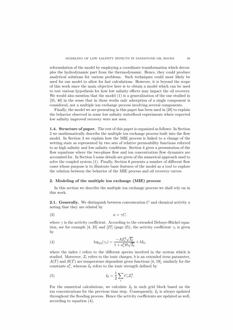
Figure 1. Plot showing βca as a function of varying Cca and Cmg

concentrations, and with Cna = 0.15 (moles per liter). Other pa-rameters in (12) like Kcana, Kmgna, and CEC, are listed in Ap-pendix A.

(12) βca(Cna, Cca, Cmg) =Kcana

√γcaCcaCEC

2Kcana

√γcaCca + 2Kmgna

√

γmgCmg + γnaCna

,

and

(13) βmg(Cna, Cca, Cmg) =Kmgna

√

γmgCmgCEC

2Kcana

√γcaCca + 2Kmgna

√

γmgCmg + γnaCna

.

We note that the equations (11), (12) and (13) are equivalent to a Langmuir-type adsorption isotherm. Fig. 1 illustrates how the βca function depends on theconcentrations Cna, Cca, Cmg. At high magnesium concentration, the amount ofcalcium ion adsorbed on the rock, βca, becomes quite low.

3. Coupling of wettability alteration to changes on the rock surface

This section discusses aspects concerning the flow functions. Since we only con-sider flows without capillary pressure in Section 6, we limit the discussion to therelative permeability functions. The following ideas are also employed in [14, 15],however, in the context of spontaneous imbibition on chalk cores where capillaryforces are the driving forces in oil recovery. It also partially follows ideas employedin previous works in [22, 41, 45].

3.1. Relative permeability functions. As a basic model for relative permeabil-ity functions the well-known Corey type correlations are used [12]. They are givenin the form (dimensionless functions)

k(s) = k∗( s− swr

1− sor − swr

)Nk

, swr ≤ s ≤ 1− sor,

ko(s) = k∗o

( 1− sor − s

1− sor − swr

)Nko

, swr ≤ s ≤ 1− sor,

(14)


where swr and sor represent critical saturation values and Nk and Nko are theCorey exponents that must be specified. In addition, k∗ and k∗o are the end pointrelative permeability values that also must be given. Now, we define two extremerelative permeability functions corresponding to the wetting state of the rock forhigh salinity and low salinity conditions.

3.1.1. High salinity conditions. This is assumed to be the initial state of thecore. The values for generating the functions are listed in Appendix B. Applying thevalues of the high salinity condition in (14) the following two relative permeabilitycurves are obtained

(15) kHS(s; sHSwr , s

HSor ), kHS

o (s; sHSwr , s

HSor ), for sHS

wr ≤ s ≤ 1− sHSor .

We refer to Fig. 2 for a plot of these curves (red line).

3.1.2. Low salinity conditions. This wetting condition is assumed to be at-tained only when there is complete desorption of Ca2+ and Mg2+ ions from therock surface. The values for generating the functions are listed in Appendix B. Ap-plying the values of the low salinity condition in (14) gives corresponding relativepermeability curves

(16) kLS(s; sLSwr , s

LSor ), kLS

o (s; sLSwr , s

LSor ), for sLS

wr ≤ s ≤ 1− sLSor .

We refer to Fig. 2 for a plot of these curves (blue line). The motivation for thechoice of the values was to match the form of the relative permeability measuredfor a variety of high salinity and low salinity brines in [43].

3.2. Cation exchange as a mechanism for wettability alteration. We letβca0 and βmg0 be the amount of calcium and magnesium, respectively, initiallybounded to the clay surface. We then define the quantity

(17) m(βca, βmg) := max(βca0 − βca, 0) + max(βmg0 − βmg, 0),

as a measure for the desorption of cations from the clay. Moreover, we define

(18) H(βca, βmg) :=1

1 + rm(βca, βmg),

where r > 0 is a specified constant. Note that the choice of r determines the extentin which the divalent ion desorbed leads to a certain change of the wetting state.

The function H(βca, βmg) is a weighting function, and works such that H = 1,when there is no desorption of calcium and magnesium from the rock, whereas 0 <

H < 1 in case of desorption of at least one of these cations. How fast H(βca, βmg)is approaching 0 as m(βca, βmg) is increasing, depends on the choice of r. Now,the weighting function H(βca, βmg) can be used to represent the wetting state inthe core plug; H(βca, βmg) = 1 corresponds to the initial oil-wet state, whereasH(βca, βmg) ≈ 0 represents the water-wet state. By defining relative permeabilitycurves by means of the weighting function H(βca, βmg) as described in the nextsubsection, the model can account for a dynamic change from an initial high salinitystate towards a low salinity state controlled by the degree of desorption of calciumand magnesium from the core.


0 0.1 0.2 0.3 0.4 0.5 0.6 0.7 0.8 0.9 10

0.1

0.2

0.3

0.4

0.5

0.6

0.7

0.8

0.9

Water Saturation

Rela

tive p

erm

eabili

ty

krw−HSkro−HSkrw−LSkro−LS

0 0.2 0.4 0.6 0.8 10

0.2

0.4

0.6

0.8

1

Water Saturation

fra

ctio

na

l flo

w

HSLS

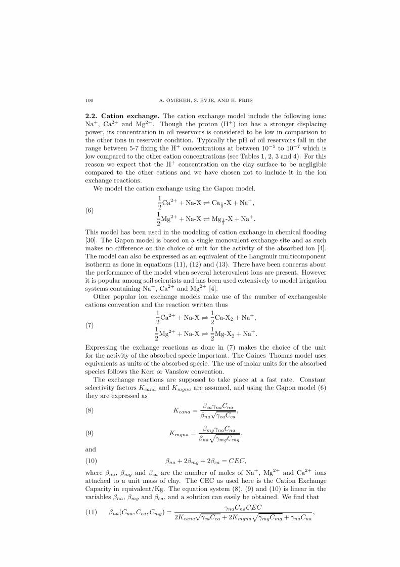
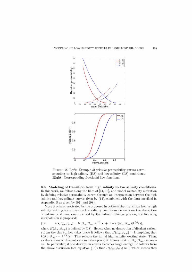
Figure 2. Left: Example of relative permeability curves corre-sponding to high-salinity (HS) and low-salinity (LS) conditions.Right: Corresponding fractional flow functions.

3.3. Modeling of transition from high salinity to low salinity conditions.In this work, we follow along the lines of [14, 15], and model wettability alterationby defining relative permeability curves through an interpolation between the highsalinity and low salinity curves given by (14), combined with the data specified inAppendix B as given by (97) and (98).

More precisely, motivated by the proposed hypothesis that transition from a highsalinity wetting state towards low salinity conditions depends on the desorptionof calcium and magnesium caused by the cation exchange process, the followinginterpolation is proposed:

(19) k(s, βca, βmg) = H(βca, βmg)kHS(s) + [1−H(βca, βmg)]k

LS(s),

whereH(βca, βmg) is defined by (18). Hence, when no desorption of divalent cation-s from the clay surface takes place it follows that H(βca, βmg) = 1, implying thatk(βca, βmg) = kHS(s). This reflects the initial high salinity wetting state. Then,as desorption of divalent cations takes place, it follows that m(βca, βmg) increas-es. In particular, if the desorption effects becomes large enough, it follows fromthe above discussion (see equation (18)) that H(βca, βmg) ≈ 0, which means that


k(s, βca, βmg) ≈ kLS(s), reflecting that a wettability alteration has taken placewhich results in a low salinity wetting state.

4. The coupled model for water-oil flow and multiple ion exchange

We now want to take into account convective and diffusive forces associated withthe brine as well as the oil phase. In order to include such effects we must considerthe following equations for the total concentrations ρo, ρl, ρca, ρso, ρmg, ρna, ρcl(mol per liter core):

∂tρo +∇ · (ρovo) = 0, (oil flowing through the pore space)

∂tρl +∇ · (ρlvl) = 0, (water flowing through the pore space)

∂tρna + ∂t(Mcβna) +∇ · (ρnavg) = 0, (Na+-ions in water)

∂tρcl +∇ · (ρclvg) = 0, (Cl−-ions in water)

∂tρca + ∂t(Mcβca) +∇ · (ρcavg) = 0, (Ca2+-ions in water)

∂tρso +∇ · (ρsovg) = 0, (SO2−4 -ions in water)

∂tρmg + ∂t(Mcβmg) +∇ · (ρmgvg) = 0, (Mg2+-ions in water).

(20)

Here vo, vl and vg are, respectively, the oil, water and species ”fluid” velocities,whereas Mc represents the mass of the clay. The subsequent derivation of themodel closely follows the work [14, 15], however, the water-rock chemistry in ourcurrent model is given in terms of a multiple ion exchange process (MIE), notdissolution/precipitation as in [14, 15].

Let so denote the oil saturation, i.e. the fraction of volume of the pore spacerepresented by porosity φ that is occupied by the oil phase, and s the correspondingwater saturation. The two saturations are related by the basic relation so + s = 1.Furthermore, we define the porous concentration Co associated with the oil com-ponent as the concentration taken with respect to the volume of the pore spaceoccupied by oil and represented by φso. Hence, Co and ρo are related by

(21) ρo = φsoCo.

Similarly, the porous concentrations of the various components in the water phaseare defined as the concentration taken with respect to the volume of the poresoccupied by water φs. Consequently, the porous concentrations Cl, Cna, Ccl, Cca,Cmg, and Cso are related to the total concentrations by

ρl = φsCl, ρna = φsCna, ρcl = φsCcl, ρca = φsCca, ρmg = φsCmg, ρso = φsCso.

Following, for example, [1, 2], we argue that since oil, water, and the ions inwater Na+, Cl−, Ca2+, Mg2+, and SO2−

4 flow only through the pores of the calcitespecimen, the ”interstitial” velocity vo associated with the oil, vl associated withthe water, and vg associated with the ions, have to be defined with respect to theconcentrations inside the pores, and differ from the respective seepage velocitiesVo, Vl and Vg. The velocities are related by the Dupuit-Forchheimer relations,see [1] and references therein,

(22) Vo = φsovo, Vl = φsvl, Vg = φsvg.


Consequently, the balance equations (20) can be written in the form

∂t(φsoCo) +∇ · (CoVo) = 0,

∂t(φsCl) +∇ · (ClVl) = 0,

∂t(φsCna) + ∂t(Mcβna) +∇ · (CnaVg) = 0,

∂t(φsCcl) +∇ · (CclVg) = 0,

∂t(φsCca) + ∂t(Mcβca) +∇ · (CcaVg) = 0,

∂t(φsCso) +∇ · (CsoVg) = 0,

∂t(φsCmg) + ∂t(Mcβmg) +∇ · (CmgVg) = 0.

(23)

In order to close the system we must determine the seepage velocities Vo, Vl andVg. For that purpose we consider the concentration of the water phase (brine) C

that occupies the pore space as a mixture of water Cl and the various species Na+,Cl−, Ca2+, Mg2+, and SO2−

4 represented by Cg. In other words,

(24) Cg = Cna + Ccl + Cca + Cmg + Cso, C = Cg + Cl.

Then, we define the seepage velocity V associated with C by

(25) CV := CgVg + ClVl.

Now we are in a position to rewrite the model in terms of V and the diffusivevelocity Ug given by

(26) Ug = Vg −V.

Then the model (23) takes the form

∂t(φsoCo) +∇ · (CoVo) = 0,

∂t(φsCl) +∇ · (ClVl) = 0,

∂t(φsCna) + ∂t(Mcβna) +∇ · (CnaUg) = −∇ · (CnaV),

∂t(φsCcl) +∇ · (CclUg) = −∇ · (CclV),

∂t(φsCca) + ∂t(Mcβca) +∇ · (CcaUg) = −∇ · (CcaV),

∂t(φsCso) +∇ · (CsoUg) = −∇ · (CsoV),

∂t(φsCmg) + ∂t(Mcβmg) +∇ · (CmgUg) = −∇ · (CmgV).

(27)

Furthermore, we can assume that the seepage velocity V associated with the waterphase represented by C, is given by Darcy’s law [1, 7, 26]

(28) V = −κλ(∇p− ρg∇d), λ =k

µ,

where κ is absolute permeability, k is water relative permeability, and µ is viscosity,and p pressure in water phase. Similarly, for the oil phase

(29) Vo = −κλo(∇po − ρog∇d), λo =ko

µo

.

The diffusive velocity Ug is expressed by Fick’s law by

(30) CiUg = −D∇Ci, i = na, cl, ca, so,mg,

where D is the diffusion coefficient. In view of (24) and (30), it follows that

(31) CgUg = −D∇Cg.

Note that we assume that the diffusion coefficient D is the same for all speciesi = na, cl, ca, so,mg. This is a reasonable assumption as long as the concentration


is not too high. D is the diffusion coefficient (longitudinal and transversal dis-persion lengths are here taken to be equal), which is split into molecular diffusioncontribution and the so called mechanical/advective contribution. A widely quotedformulation by Sahimi [32] is of the form

(32)D

Dm

= φpsq + aPe + bP δe + cP 2

e ,

where Dm is the free molecular diffusion coefficient, p, q, a, b, c, and δ are experi-mentally determined constants and Pe is the Peclet number given by

(33) Pe =α|V|Dm

,

where α is the characteristic dispersion length which varies from millimeters (inlaboratory scale) to metres(field scale). Several authors [8, 32] have experimentallydetermined that the diffusion co-efficient is determined by only the first term ofequation(32) when Pe is less than 0.3, and a transition zone between 0.3 and 5where D is not clearly defined. The other terms of the equation becomes significantat higher Peclet numbers. For our application of the model, the Peclet number fallsbelow 0.3, hence subsequently we use only the first term of equation (32). In (32)the coefficient p is referred to as the cementation exponent, q as the saturationexponent. The cementation exponent is often close to 2 whereas the saturationexponent is also often fixed at a value in the same range, see for example [8, 10, 11].Using (30) in (27) yields

∂t(φsoCo) +∇ · (CoVo) = 0,

∂t(φsCl) +∇ · (ClVl) = 0,

∂t(φsCna) + ∂t(Mcβna)−∇ · (D∇Cna) = −∇ · (CnaV),

∂t(φsCcl)−∇ · (D∇Ccl) = −∇ · (CclV),

∂t(φsCca) + ∂t(Mcβca)−∇ · (D∇Cca) = −∇ · (CcaV),

∂t(φsCso)−∇ · (D∇Cso) = −∇ · (CsoV),

∂t(φsCmg) + ∂t(Mcβmg)−∇ · (D∇Cmg) = −∇ · (CmgV).

(34)

In particular, summing the equations corresponding to Cna, Ccl, Cca, Cso, andCmg, we obtain an equation for Cg in the form

(35) ∂t(φsCg) + ∂t(Mc[βna + βca + βmg])−∇ · (D∇Cg) = −∇ · (CgV).

In a similar manner, using ClVl = ClV − CgUg (obtained from (25), (26), and(24)) in the second equation of (34), the following equation is obtained

∂t(φsCl) +∇ · (ClV) = ∇ · (CgUg).(36)

Summing (36) and (35), we get the following equation for the concentration of thewater phase with its different chemical components, represented by C = Cg + Cl,

(37) ∂t(φsC) + ∂t(Mc[βna + βca + βmg]) +∇ · (CV) = 0.


To sum up, we have a model in the form

∂t(φsoCo) +∇ · (CoVo) = 0,

∂t(φsC) + ∂t(Mc[βna + βca + βmg]) +∇ · (CV) = 0,

∂t(φsCna) + ∂t(Mcβna) +∇ · (CnaV) = ∇ · (D∇Cna),

∂t(φsCcl) +∇ · (CclV) = ∇ · (D∇Ccl),

∂t(φsCca) + ∂t(Mcβca) +∇ · (CcaV) = ∇ · (D∇Cca),

∂t(φsCso) +∇ · (CsoV) = ∇ · (D∇Cso),

∂t(φsCmg) + ∂t(Mcβmg) +∇ · (CmgV) = ∇ · (D∇Cmg),

(38)

where D = D(φ, s) as given by (32).

4.1. Simplifying assumptions. Before we proceed some simplifying assumptionsare made:

• The oil and water component densities Co and C are assumed to be con-stant, i.e., incompressible fluids;

• The effect from the water-rock chemistry in the water phase equation (sec-ond equation of (38)) is neglected which is reasonable since the concentra-tion of the water phase C is much larger than the concentrations of the ionexchange involved in the chemical reactions;

• Constant porosity φ, absolute permeability κ, viscosities µ, µo;• One dimensional flow in a horizontal domain.• Capillary pressure is currently neglected as discussed in the introduction(Section 1.2).

This results in the following simplified model:

∂t(φso) + ∂x(Vo) = 0,

∂t(φs) + ∂x(V ) = 0,

∂t(φsCna) + ∂t(Mcβna) + ∂x(CnaV ) = ∂x(D(φ, s)∂xCna),

∂t(φsCcl) + ∂x(CclV ) = ∂x(D(φ, s)∂xCcl),

∂t(φsCca) + ∂t(Mcβca) + ∂x(CcaV ) = ∂x(D(φ, s)∂xCca),

∂t(φsCso) + ∂x(CsoV ) = ∂x(D(φ, s)∂xCso),

∂t(φsCmg) + ∂t(Mcβmg) + ∂x(CmgV ) = ∂x(D(φ, s)∂xCmg).

(39)

In view of (28) and (29) in a 1D domain, we get

V =− κλpx, λ(βca, βmg) =k(βca, βmg)

µ(40)

Vo =− κλopo,x, λo(βca, βmg) =ko(βca, βmg)

µo

,(41)

Moreover, capillary pressure Pc is defined as the difference between oil and waterpressure

(42) Pc = po − p,

and is assumed to be zero in the following. Total velocity vT is given by

vT := V + Vo = −κ(λpx + λopo,x) = −κλT px,(43)

where total mobility λT

(44) λT = λ+ λo,


has been introduced. Summing the two first equations of (39) and using that1 = s + so, implies that (vT )x = 0, i.e., vT =constant and is determined, forexample, from the boundary conditions. From the continuity equation for s givenby the second equation of (39) it follows (since V = −κλpx)

(45) (φs)t + (−κλpx)x = 0,

where, in view of (43),

−κpx =vT

λT

.

Thus,

(φs)t + (vTλ

λT

)x = 0.(46)

The fractional flow functions f(βca, βmg) and fo(βca, βmg) are defined as follows

f(s, βca, βmg)def:=

λ(s, βca, βmg)

λ(s, βca, βmg) + λo(βca, βmg),(47)

fo(s, βca, βmg)def:=

λo(s, βca, βmg)

λ(s, βca, βmg) + λo(βca, βmg)= 1− f(βca, βmg).(48)

Using this in (46) implies that

(49) (φs)t + vT f(s, βca, βmg)x = 0.

The same procedure can be applied for the continuity equation for the differentions in water in (39). This gives the following equation for i = na, cl, ca, so,mg:

(φsCi)t + (Mcβi)t + vT (Cif(s, βca, βmg)x = (D(φ, s)Ci,x)x, i = na, cl, ca, so,mg.

(50)

Thus, in view of (49) and (50), a model has been obtained of the form

∂t(φs) + vT ∂xf(s, βca, βmg) = 0,(51)

∂t(φsCna +Mcβna) + vT∂x(Cnaf(s, βca, βmg)) = ∂x(D(φ, s)∂xCna),

∂t(φsCcl) + vT∂x(Cclf(s, βca, βmg)) = ∂x(D(φ, s)∂xCcl),

∂t(φsCca +Mcβca) + vT ∂x(Ccaf(s, βca, βmg)) = ∂x(D(φ, s)∂xCca)

∂t(φsCso) + vT∂x(Csof(s, βca, βmg)) = ∂x(D(φ, s)∂xCso),

∂t(φsCmg +Mcβmg) + vT∂x(Cmgf(s, βca, βmg)) = ∂x(D(φ, s)∂xCmg).

4.2. Scaled version of the model. First, we introduce the variables

c1 := φsCna, c2 := φsCcl, c3 := φsCca, c4 := φsCso, c5 := φsCmg .(52)

We also introduce the variables(53)B1 = Mcβna(Cna, Cca, Cmg), B3 = Mcβca(Cna, Cca, Cmg), B5 = Mcβmg(Cna, Cca, Cmg).

Now let L be the the reference length, which here is chosen to be the length of the core.As time scale of the problem τ (sec) we use

(54) τ =φL

vT.

We then define dimensionless space x′ and time t′ variables as follows

(55) x′ =x

L, t′ =

t

τ.


We introduce reference viscosity µ (Pa s), and reference diffusion coefficient Dm (m2/s).Then we define dimensionless coefficients

(56) D′m =

Dm

Dm

, µ′ =µ

µ.

Rewriting (51) in terms of the dimensionless space and time variables (55) and using (56),the following form of the system is obtained (skipping the prime notation)

∂t(φs) + ∂x(φf(s, βca, βmg)) = 0,(57)

∂t(c1 +B1(c1, c3, c5)) + ∂x(Cnaφf(s, βca, βmg)) = δ∂x(Dmφpsq∂xCna),

∂t(c2) + ∂x(Cclφf(s, βca, βmg)) = δ∂x(Dmφpsq∂xCcl),

∂t(c3 +B2(c1, c3, c5)) + ∂x(Ccaφf(s, βca, βmg)) = δ∂x(Dmφpsq∂xCca),

∂t(c4) + ∂x(Csoφf(s, βca, βmg)) = δ∂x(Dmφpsq∂xCso),

∂t(c5 +B3(c1, c3, c5)) + ∂x(Cmgφf(s, βca, βmg)) = δ∂x(Dmφpsq∂xCmg),

(58)

where the dimensionless characteristic number δ, is given by

(59) δ =φDm

LvT.

We choose Dm = LvT in (56) such that δ = φ.

4.3. Boundary and initial conditions. In order to have a well defined system to solvewe must specify appropriate initial and boundary conditions.

4.3.1. Boundary conditions. At the inlet, the following Dirichlet boundary conditionsare employed

(60) s(0−, t) = s(1+, t) = 1.0, Ci(0−, t) = Ci(1

+, t) = C∗i ,

for the species i = na, cl, ca, so,mg where C∗i is the specified ion concentrations of the

brine that is used. At the outlet extrapolation is employed both for s and the Ci’s.

4.3.2. Initial data. Initially, the plug is filled with oil and 15.0% formation water. Thus,initial data are given by

(61) s|t=0(x) = sinit = 0.15, x ∈ [0, 1],

and for i = na, cl, ca, so,mg,

(62) Ci|t=0(x) = Ci,0, x ∈ [0, 1],

for given initial concentration of the species Ci,0 in the water phase (formation water).

5. Numerical discretization

The numerical discretization of the resulting nonlinear convection-diffusion system isbased on the same approach as that used in [45, 46], and we refer to these works for moredetails. However, for completeness we briefly sketch the discretization of the nonlinearconvective term. The diffusion term is discretized by using a standard central discretiza-tion.

5.1. Discretization of convective flux. Consider now a system of conservation lawsin one space variable

∂tw + ∂xF (w) = 0,(63)

where F (w) ∈ Rn is a smooth vector-valued function. The discretization of the nonlinear

convective (advective) flux is based on the relaxed scheme by Jin and Xin [23]. The relaxedscheme can be written in the following ”viscous” form

wn+1j = wn

j − λ(Fnj+1/2 − Fn

j−1/2), λ = ∆t∆x

where

Fj+1/2 = 12

(F (wj) + F (wj+1)

)− 1

2A1/2(wj+1 −wj),

(64)


where A1/2 plays the role as the “viscosity matrix” which determines the numerical dissipa-tion of the scheme. Here we must require that the well known subcharacteristic conditionholds given by

A− F ′(w)2 ≥ 0, for all w.(65)

In our case it suffices to choose that A has the special form

A = aI, a > 0(66)

where I is the identity matrix. In the case of one space variable (as we consider) andwhere we assume (66), the dissipative condition (65) is satisfied if

λ2 < a,(67)

where λ = max1≤i≤n |λi(w)| where λi are the genuine eigenvalues of F ′(w).The relaxed scheme (64) can also be viewed as a flux splitting scheme. To see this we

write the system as

wn+1j = wn

j − λ(Fnj+1/2 − Fn

j−1/2)

where

Fj+1/2 = F+j+1/2,−

+ F−j+1/2,+

,

(68)

where we have (for the first order scheme) that

F+j+1/2,− = F+(wj), F−

j+1/2,+ = F−(wj+1),

and where we have used the Lax-Friedrichs flux splitting

F±(w) =1

2(F (w)±A1/2

w).(69)

Note that the condition (65) ensures that the Jacobian of F±(w) has nonnegative eigen-values only or nonpositive eigenvalues only.

The second order relaxed scheme can be obtained by using van Leer’s MUSCL scheme.Instead of using the piecewise constant interpolation, MUSCL uses the piecewise linearinterpolation which, when it is applied to the p-th components of F+(wj) approximatedat xj , yields:

(F+)(p)j (x) = (F+)(p)(wj) + (S+)

(p)j (x− xj), x ∈ (xj−1/2, xj+1/2)

where

(S+)(p)j = S((s+l )

(p), (s+r )(p))

(70)

and

(s+l )p =

(F+)(p)(wj)− (F+)(p)(wj−1)

∆x, (s+r )

p =(F+)(p)(wj+1)− (F+)(p)(wj)

∆x.

Here S(u, v) represents the slope limiter function. Similarly, the piecewise linear interpo-lation applied to the p-th components of the negative flux part F−(wj+1) approximatedat xj+1 yields:

(F−)(p)j+1(x) = (F−)(p)(wj+1) + (S−)

(p)j+1(x− xj+1), x ∈ (xj+1/2, xj+3/2)

where

(S−)(p)j+1 = S((s−l )

(p), (s−r )(p))

(71)

and

(s−l )p =

(F−)(p)(wj+1)− (F−)(p)(wj)

∆x, (s−r )

p =(F−)(p)(wj+2)− (F−)(p)(wj+1)

∆x.

The van Leer limiter corresponds to the choice

S(u, v) = s(u, v)2|u||v||u|+ |v| ,(72)


where s(u, v) = 1/2(sgn(u) + sgn(v)). The numerical flux F(p)

j+1/2 is then computed in a

split form,

F(p)

j+1/2= (F+)

(p)j (x)|xj+1/2

+ (F−)(p)j+1(x)|xj+1/2

.(73)

Second order accuracy in time can be obtained by using a two-stage Runge-Kutta dis-cretization. We chose to employ a standard forward Euler since this required less timeand main purpose of simulations was to evaluate impact from the ion exchange processon the two-phase flow behavior.

5.2. Generally. A main difference between the current model and the one discussed in[45] is that a more complicated nonlinear system of algebraic equations must be solveddue to the multiple ion exchange process. In contrast, [45, 46] considered only a singleadsorption isotherm. In order to describe this more precisely, let us introduce the vector

(74) E = (c1 +B1(c1, c3, c5, φs), c2, c3 +B3(c1, c3, c5, φs), c4, c5 +B5(c1, c3, c5, φs))T ,

and

(75) C = (c1, c2, c3, c4, c5)T .

We assume that we have approximate solutions (sn,Cn)(·) ≈ (s,C)(·, tn). Now, we wantto calculate an approximation at the next time level (sn+1,Cn+1)(·) ≈ (s,C)(·, tn+1). Thesystem of parabolic PDEs given by equations (57) and (58), which we solve for t ∈ (0,∆t],is in the form

∂ts+ ∂xf(s,C) = 0, s(·, 0) = sn(·),∂tE+ ∂xF(s,C) = ∂x(D(s)∂x(C/s)), C(·, 0) = C

n(·),(76)

for suitable choices of F and D. Then we find (sn+1,En+1). Finally, in order to proceedto the next time step, we must compute Cn+1 = H(En+1), where the latter equation is anonlinear algebraic equation, which can be written as(77)

(c1+B1(c1, c3, c5, φsn+1), c2, c3+B3(c1, c3, c5, φs

n+1), c4, c5+B5(c1, c3, c5, φsn+1))T = E

n+1.

Note that the above equations are nonlinear in the variables c1, c3 and c5, but is a straight-forward identity for c2 and c4. By solving equation (77) numerically, we obtain Cn+1. Wedescribe the procedure in the next subsection. However, we should also note that thechemical activity coefficients γi = γi(I0) for species i, are updated before every new timestep in our numerical procedure by using the concentrations Cna, Ccl, Cca, Cso, Cmg ob-tained from C, in equations (4) and (5), as explained in Section 2.1.

5.3. Solving the nonlinear system. It is seen by looking at the equations (11), (12)and (13), and using the definition (53) that

(78) B1 = C1c1√c3

B3,

and

(79) B5 = C3

√c5√c3

B3,

where

(80) C1 =γna√

φsn+1γcaKcana

,

and

(81) C3 =

√γmgKmgna√γcaKcana

.

Now using (78) as well as the first and third equations in (77), it is easily found that

(82) c1 =

√xEn+1

1√x+ C1(E

n+13 − x)

,


where we have set x := c3. Likewise, (79) can be used in combination with the third andfifth equations in (77) to establish the equation

(83) c5√x+ C3(E

n+13 − x)

√c5 = En+1

5

√x.

We note from (83) that if x is equal to zero then c5 = 0. If x > 0 then let

(84) B =C3(E

n+13 − x)√x

,

and

(85) w =√c5, (c5 = w2),

in order to obtain the second order equation

(86) w2 + Bw − En+15 = 0,

which has the physical solution

(87) w = w(x) =−B(x) +

√B(x)2 + 4En+1

5

2.

Finally, using the third equation in (77) i.e.

(88) x+B3(c1(x), x, c5(x), φsn+1) = En+1

3 ,

and substituting the expressions for c1(x) and c5(x), found from the equations (82), (85),and (87) above, in B3, we arrive at the following nonlinear equation in the variable x (inlight of (12) and (52)):

(89) x+g(x)

h(x)− En+1

3 = 0,

where

(90) g(x) = McCEC√γcaKcana

√x,

and

h(x) = 2Kcana√γca

√x+

γna√φsn+1

( √xEn+1

1√x+ C1(E

n+13 − x)

)

+ Kmgna√γmg

(− C3(E

n+13 − x)√x

+

√(C3(E

n+13 − x))2

x+ 4En+1

5

).(91)

Currently, we solve the nonlinear equation (89) by using the matlab routine fzero.

5.4. Numerical treatment of the selectivity factors. A number of authors haveshown that the selectivity factors may vary with brine salinity and concentrations in acomplex way. See [4, 20] for examples of such relations. For the MIE model representedby (6) we see that the selectivity factors we have to deal with are Kcana and Kmgna.For ease of computations we interpolate linearly between two extreme values of selectivityfactors KLS

mgna and KHSmgna, corresponding to low salinity brine concentrations BLS

s and

high salinity brine concentrations BHSs respectively:

Kmgna(Bs) =( BHS

s −Bs

BHSs −BLS

s

)KLS

mgna +( Bs −BLS

s

BHSs −BLS

s

)KHS

mgna

Kcana(Bs) =( BHS

s −Bs

BHSs −BLS

s

)KLS

cana +( Bs −BLS

s

BHSs −BLS

s

)KHS

cana,

(92)

where Brine salinity Bs is given by

(93) Bs =∑

i

CiZi.

Note that the selectivity factors are updated at each grid block for every new time stepby using values of the brine salinity from the previous time step. We refer to AppendixA for specific choices of BLS

s and BHSs as well as KLS

mgna,KHSmgna and KLS

cana,KHScana.


0 0.1 0.2 0.3 0.4 0.5 0.6 0.7 0.8 0.9 10

0.1

0.2

0.3

0.4

0.5

0.6

0.7

0.8

0.9

1

Sw

Dimensionless distance

Water Saturation

40cells120cells

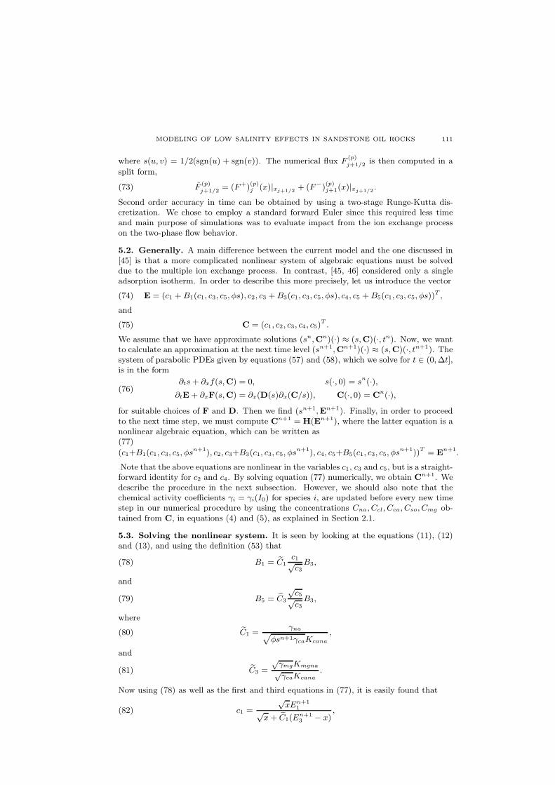
Figure 3. Saturation profiles computed with 40 and 120 grid cells,respectively. The comparison is taken from SW flooding (Example1, case 2).

6. Numerical investigations

6.1. Generally. The core plug under consideration is initially filled with formation waterwhich is in equilibrium with the ions on the rock surface. Initially, the core plug has a givenwetting state, termed here as high salinity wetting state, which is completely describedby its relative permeability functions, see Section 3.1. However, when flooding is donewith a brine with ion concentrations different from the formation water, the invadingbrine creates concentration fronts that move with a certain speed. At these fronts, aswell as behind them, chemical interactions in terms of a multiple ion exchange processwill take place. It is expected that the water-rock interaction then can lead to a changeof the wetting state such that more oil can be mobilized. Main focus of this paper hasbeen, motivated by previous experimental research as described in Section 1, to buildinto the model a mechanism that relates wettability alteration (towards a low salinitywetting state) to desorption of divalent cations from the rock surface. The purpose ofthis computational section is to gain some general insight into the behavior of this model,when performing water flooding with different brines. Obviously, we are particularlyinterested to see whether we can discover any ”low salinity effects” on the oil recoverycurves produced by the numerical model.

6.2. Various data needed for the water flooding simulations. A range of inputparameters must be specified for the above model, and are given in Appendix A and B. Weemphasize that we will use a fixed set of parameters for all simulations, unless anything elseis clearly stated. The only change from one simulation to another is the brine compositionand/or formation water composition (initial condition).

6.3. A remark on the numerical resolution in the simulations. As stated earlier,the equation systems are solved explicitly. We think that the solutions provided by theexplicit method in this paper are sufficient for our present purpose, since we are inter-ested in investigating the fundamental behavior of our one dimensional model. We firstpresent a simulation case where we demonstrate convergence of the numerical solution.We have considered formation water FW and flooding water SW with ion concentrationsas described in Table 2 in Appendix A. We have computed solutions on a grid of 40 cellsand 120 cells, respectively. Result for the water saturation at different times is shown inFig. 3. We conclude that it is sufficient to compute solutions on a grid of 40 cells. Thiswill be done in the remaining part of the work.


0 1 2 3 4 5 60

0.1

0.2

0.3

0.4

0.5

0.6

0.7

0.8

0.9

Time (days)

oil r

ecov

ery

Recovery

LSHS

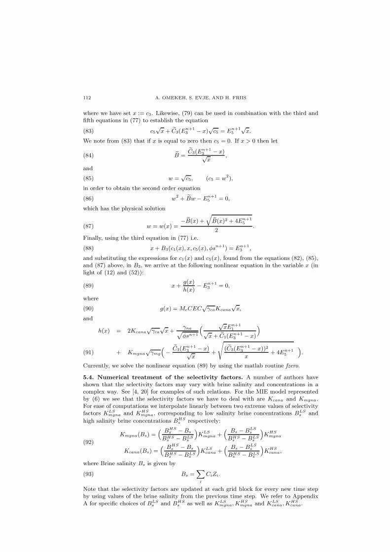
Figure 4. Plot showing the recoveries for HS and LS relative per-meability curves given in Fig. 2.

0 0.5 1

4

6

8

10

12

14

x 10−4


BetaMg

0 0.5 10

0.5

1

1.5

2

2.5

3

3.5

4

4.5x 10

−3


BetaCa

0 0.5 1

2

4

6

8

10

12x 10

−3


BetaNa

Initial0.133days0.3330.6671.3332.0004.0006.000

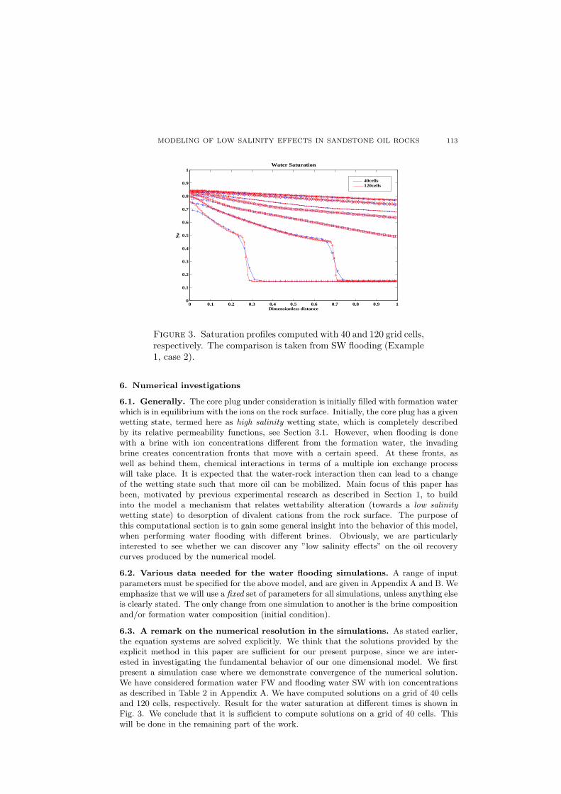
Figure 5. Plots showing the behavior of the various β-functionsalong the core at different times during a time period of 6 days,for the case with LSW as the invading low salinity brine. Notethat there is no desorption of the divalent ions (calcium and mag-nesium), only adsorption. Left: βmg. Middle: βca. Right: βna.

Before we start exploring how oil recovery can be sensitive for the brine composition ofthe water that is used for flooding, we show two extremes: Oil recovery for the high salinityconditions represented by relative permeability curves (15) versus oil recovery for the lowsalinity conditions represented by relative permeability curves (16). See also Appendix Bfor specific data used for the relative permeability functions. Results are shown in Fig. 4.This information is useful to have in mind when we in the remaining part of this sectionconsider brine-dependent oil recovery curves.

6.4. Example 1: Water flooding using different brines and fixed formation

water. Here we present simulations of corefloods. The core is composed of clay and otherminerals that are assumed to be relatively chemically nonreactive typical of sandstone


0 0.2 0.4 0.6 0.8 10

0.005

0.01

0.015

0.02


Mg Concentration

Co

nce

ntr

atio

n m

ol/L

0 0.2 0.4 0.6 0.8 10

0.05

0.1

0.15

0.2


Ca Concentration

Co

nce

ntr

atio

n m

ol/L

0 0.2 0.4 0.6 0.8 10

0.5

1

1.5


Na Concentration

Co

nce

ntr

atio

n m

ol/L

0 0.2 0.4 0.6 0.8 10

0.5

1

1.5

2


Cl Concentration

Co

nce

ntr

atio

n m

ol/L

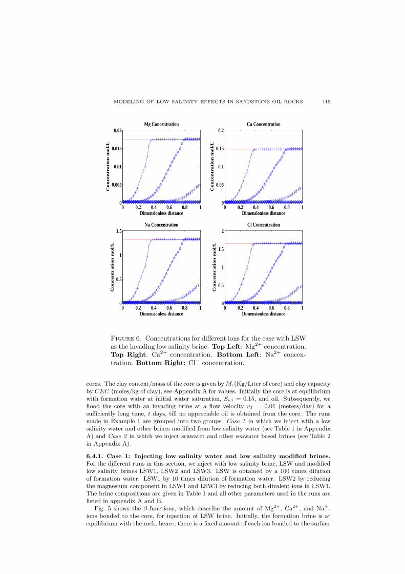
Figure 6. Concentrations for different ions for the case with LSWas the invading low salinity brine. Top Left: Mg2+ concentration.Top Right: Ca2+ concentration. Bottom Left: Na2+ concen-tration. Bottom Right: Cl− concentration.

cores. The clay content/mass of the core is given byMc(Kg/Liter of core) and clay capacityby CEC (moles/kg of clay), see Appendix A for values. Initially the core is at equilibriumwith formation water at initial water saturation, Swi = 0.15, and oil. Subsequently, weflood the core with an invading brine at a flow velocity vT = 0.01 (meters/day) for asufficiently long time, t days, till no appreciable oil is obtained from the core. The runsmade in Example 1 are grouped into two groups: Case 1 in which we inject with a lowsalinity water and other brines modified from low salinity water (see Table 1 in AppendixA) and Case 2 in which we inject seawater and other seawater based brines (see Table 2in Appendix A).

6.4.1. Case 1: Injecting low salinity water and low salinity modified brines.

For the different runs in this section, we inject with low salinity brine, LSW and modifiedlow salinity brines LSW1, LSW2 and LSW3. LSW is obtained by a 100 times dilutionof formation water. LSW1 by 10 times dilution of formation water. LSW2 by reducingthe magnesium component in LSW1 and LSW3 by reducing both divalent ions in LSW1.The brine compositions are given in Table 1 and all other parameters used in the runs arelisted in appendix A and B.

Fig. 5 shows the β-functions, which describe the amount of Mg2+, Ca2+, and Na+-ions bonded to the core, for injection of LSW brine. Initially, the formation brine is atequilibrium with the rock, hence, there is a fixed amount of each ion bonded to the surface


0 0.2 0.4 0.6 0.8 10

0.1

0.2

0.3

0.4

0.5

0.6

0.7

0.8

0.9

1


H function

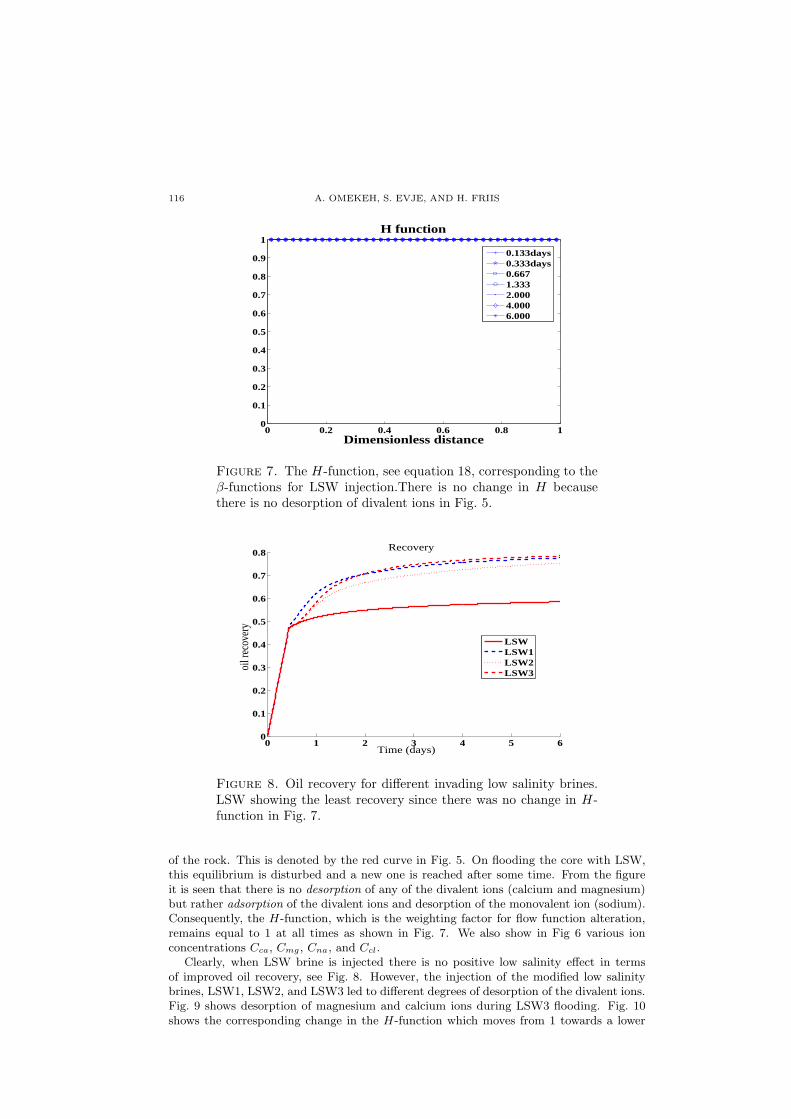
0.133days0.333days0.6671.3332.0004.0006.000

Figure 7. The H-function, see equation 18, corresponding to theβ-functions for LSW injection.There is no change in H becausethere is no desorption of divalent ions in Fig. 5.

0 1 2 3 4 5 60

0.1

0.2

0.3

0.4

0.5

0.6

0.7

0.8

Time (days)

oil r

ecov

ery

Recovery

LSWLSW1LSW2LSW3

Figure 8. Oil recovery for different invading low salinity brines.LSW showing the least recovery since there was no change in H-function in Fig. 7.

of the rock. This is denoted by the red curve in Fig. 5. On flooding the core with LSW,this equilibrium is disturbed and a new one is reached after some time. From the figureit is seen that there is no desorption of any of the divalent ions (calcium and magnesium)but rather adsorption of the divalent ions and desorption of the monovalent ion (sodium).Consequently, the H-function, which is the weighting factor for flow function alteration,remains equal to 1 at all times as shown in Fig. 7. We also show in Fig 6 various ionconcentrations Cca, Cmg , Cna, and Ccl.

Clearly, when LSW brine is injected there is no positive low salinity effect in termsof improved oil recovery, see Fig. 8. However, the injection of the modified low salinitybrines, LSW1, LSW2, and LSW3 led to different degrees of desorption of the divalent ions.Fig. 9 shows desorption of magnesium and calcium ions during LSW3 flooding. Fig. 10shows the corresponding change in the H-function which moves from 1 towards a lower


0 0.5 1

4

6

8

10

12

14

x 10−4


BetaMg

0 0.5 10

0.5

1

1.5

2

2.5

3

3.5

4

4.5x 10

−3


BetaCa

0 0.5 1

2

4

6

8

10

12x 10

−3


BetaNa

Initial0.1333days0.33330.66671.33332.00004.00006.0000

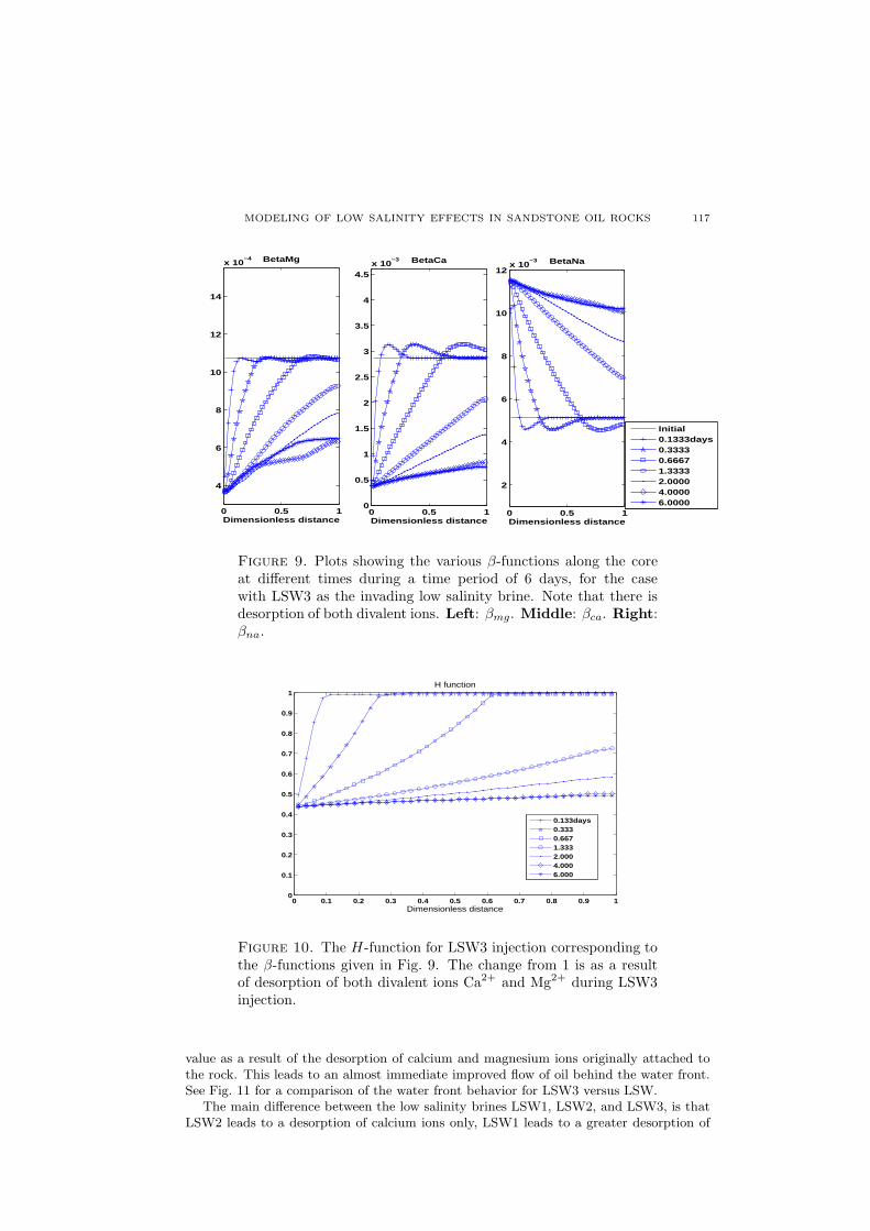
Figure 9. Plots showing the various β-functions along the coreat different times during a time period of 6 days, for the casewith LSW3 as the invading low salinity brine. Note that there isdesorption of both divalent ions. Left: βmg. Middle: βca. Right:βna.

0 0.1 0.2 0.3 0.4 0.5 0.6 0.7 0.8 0.9 10

0.1

0.2

0.3

0.4

0.5

0.6

0.7

0.8

0.9

1


H function

0.133days0.3330.6671.3332.0004.0006.000

Figure 10. The H-function for LSW3 injection corresponding tothe β-functions given in Fig. 9. The change from 1 is as a resultof desorption of both divalent ions Ca2+ and Mg2+ during LSW3injection.

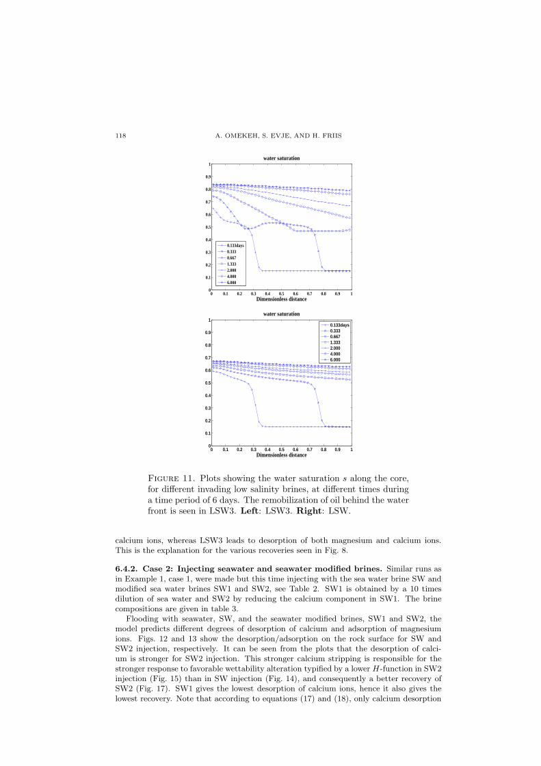
value as a result of the desorption of calcium and magnesium ions originally attached tothe rock. This leads to an almost immediate improved flow of oil behind the water front.See Fig. 11 for a comparison of the water front behavior for LSW3 versus LSW.

The main difference between the low salinity brines LSW1, LSW2, and LSW3, is thatLSW2 leads to a desorption of calcium ions only, LSW1 leads to a greater desorption of


0 0.1 0.2 0.3 0.4 0.5 0.6 0.7 0.8 0.9 10

0.1

0.2

0.3

0.4

0.5

0.6

0.7

0.8

0.9

1


water saturation

0.133days0.3330.6671.3332.0004.0006.000

0 0.1 0.2 0.3 0.4 0.5 0.6 0.7 0.8 0.9 10

0.1

0.2

0.3

0.4

0.5

0.6

0.7

0.8

0.9

1


water saturation

0.133days0.3330.6671.3332.0004.0006.000

Figure 11. Plots showing the water saturation s along the core,for different invading low salinity brines, at different times duringa time period of 6 days. The remobilization of oil behind the waterfront is seen in LSW3. Left: LSW3. Right: LSW.

calcium ions, whereas LSW3 leads to desorption of both magnesium and calcium ions.This is the explanation for the various recoveries seen in Fig. 8.

6.4.2. Case 2: Injecting seawater and seawater modified brines. Similar runs asin Example 1, case 1, were made but this time injecting with the sea water brine SW andmodified sea water brines SW1 and SW2, see Table 2. SW1 is obtained by a 10 timesdilution of sea water and SW2 by reducing the calcium component in SW1. The brinecompositions are given in table 3.

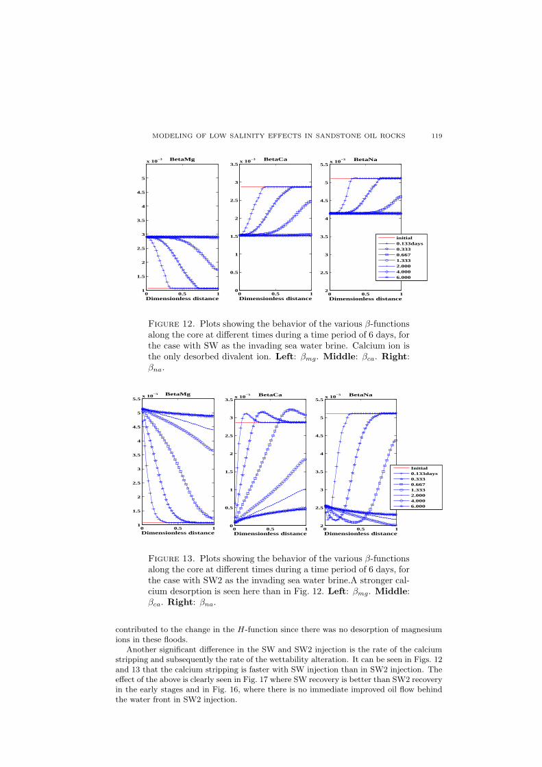
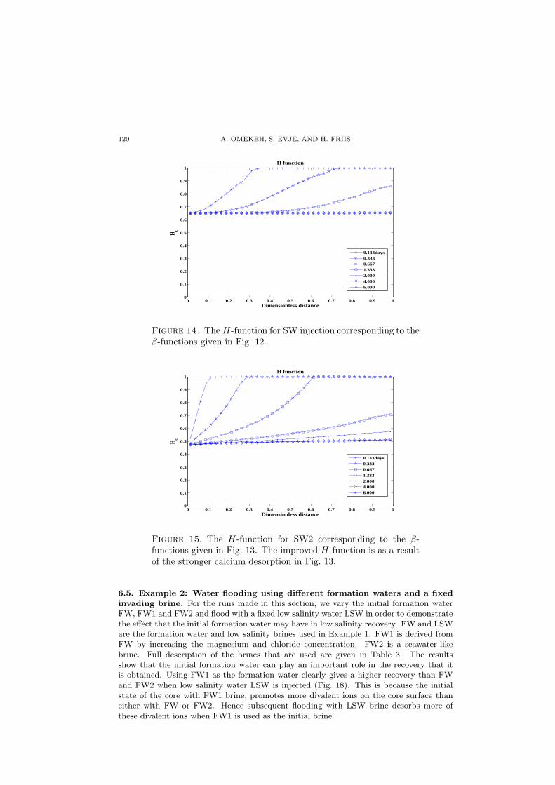
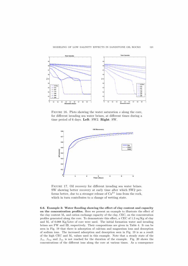
Flooding with seawater, SW, and the seawater modified brines, SW1 and SW2, themodel predicts different degrees of desorption of calcium and adsorption of magnesiumions. Figs. 12 and 13 show the desorption/adsorption on the rock surface for SW andSW2 injection, respectively. It can be seen from the plots that the desorption of calci-um is stronger for SW2 injection. This stronger calcium stripping is responsible for thestronger response to favorable wettability alteration typified by a lower H-function in SW2injection (Fig. 15) than in SW injection (Fig. 14), and consequently a better recovery ofSW2 (Fig. 17). SW1 gives the lowest desorption of calcium ions, hence it also gives thelowest recovery. Note that according to equations (17) and (18), only calcium desorption


0 0.5 11

1.5

2

2.5

3

3.5

4

4.5

5

x 10−3


BetaMg

0 0.5 10

0.5

1

1.5

2

2.5

3

3.5x 10

−3


BetaCa

0 0.5 12

2.5

3

3.5

4

4.5

5

5.5x 10

−3


BetaNa

initial0.133days0.3330.6671.3332.0004.0006.000

Figure 12. Plots showing the behavior of the various β-functionsalong the core at different times during a time period of 6 days, forthe case with SW as the invading sea water brine. Calcium ion isthe only desorbed divalent ion. Left: βmg. Middle: βca. Right:βna.

0 0.5 11

1.5

2

2.5

3

3.5

4

4.5

5

5.5x 10

−3


BetaMg

0 0.5 10

0.5

1

1.5

2

2.5

3

3.5x 10

−3


BetaCa

0 0.5 12

2.5

3

3.5

4

4.5

5

5.5x 10

−3


BetaNa

Initial0.133days0.3330.6671.3332.0004.0006.000

Figure 13. Plots showing the behavior of the various β-functionsalong the core at different times during a time period of 6 days, forthe case with SW2 as the invading sea water brine.A stronger cal-cium desorption is seen here than in Fig. 12. Left: βmg. Middle:βca. Right: βna.

contributed to the change in the H-function since there was no desorption of magnesiumions in these floods.

Another significant difference in the SW and SW2 injection is the rate of the calciumstripping and subsequently the rate of the wettability alteration. It can be seen in Figs. 12and 13 that the calcium stripping is faster with SW injection than in SW2 injection. Theeffect of the above is clearly seen in Fig. 17 where SW recovery is better than SW2 recoveryin the early stages and in Fig. 16, where there is no immediate improved oil flow behindthe water front in SW2 injection.


0 0.1 0.2 0.3 0.4 0.5 0.6 0.7 0.8 0.9 10

0.1

0.2

0.3

0.4

0.5

0.6

0.7

0.8

0.9

1H

c


H function

0.133days0.3330.6671.3332.0004.0006.000

Figure 14. TheH-function for SW injection corresponding to theβ-functions given in Fig. 12.

0 0.1 0.2 0.3 0.4 0.5 0.6 0.7 0.8 0.9 10

0.1

0.2

0.3

0.4

0.5

0.6

0.7

0.8

0.9

1

Hc


H function

0.133days0.3330.6671.3332.0004.0006.000

Figure 15. The H-function for SW2 corresponding to the β-functions given in Fig. 13. The improved H-function is as a resultof the stronger calcium desorption in Fig. 13.

6.5. Example 2: Water flooding using different formation waters and a fixed

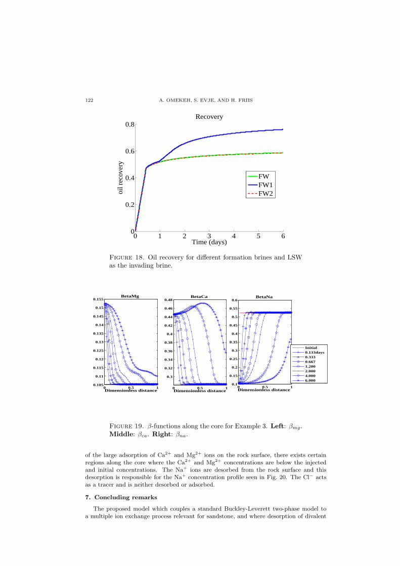
invading brine. For the runs made in this section, we vary the initial formation waterFW, FW1 and FW2 and flood with a fixed low salinity water LSW in order to demonstratethe effect that the initial formation water may have in low salinity recovery. FW and LSWare the formation water and low salinity brines used in Example 1. FW1 is derived fromFW by increasing the magnesium and chloride concentration. FW2 is a seawater-likebrine. Full description of the brines that are used are given in Table 3. The resultsshow that the initial formation water can play an important role in the recovery that itis obtained. Using FW1 as the formation water clearly gives a higher recovery than FWand FW2 when low salinity water LSW is injected (Fig. 18). This is because the initialstate of the core with FW1 brine, promotes more divalent ions on the core surface thaneither with FW or FW2. Hence subsequent flooding with LSW brine desorbs more ofthese divalent ions when FW1 is used as the initial brine.


0 0.1 0.2 0.3 0.4 0.5 0.6 0.7 0.8 0.9 10

0.1

0.2

0.3

0.4

0.5

0.6

0.7

0.8

0.9

1

Sw


Water Saturation

0.133days0.3330.6671.3332.0004.0006.000

0 0.1 0.2 0.3 0.4 0.5 0.6 0.7 0.8 0.9 10

0.1

0.2

0.3

0.4

0.5

0.6

0.7

0.8

0.9

1

Sw


Water Saturation

0.133days0.3330.6671.3332.0004.0006.000

Figure 16. Plots showing the water saturation s along the core,for different invading sea water brines, at different times during atime period of 6 days. Left: SW2. Right: SW.

0 1 2 3 4 5 60

0.1

0.2

0.3

0.4

0.5

0.6

0.7

0.8

Time (days)

oil r

ecov

ery

Oil Recovery

SwSW1SW2

Figure 17. Oil recovery for different invading sea water brines.SW showing better recovery at early time after which SW2 per-forms better, due to a stronger release of Ca2+ ions from the rock,which in turn contributes to a change of wetting state.

6.6. Example 3: Water flooding showing the effect of clay content and capacity

on the concentration profiles. Here we present an example to illustrate the effect ofthe clay content Mc and cation exchange capacity of the clay, CEC, on the concentrationprofiles generated along the core. To demonstrate this effect, a CEC of 1.3 eq/Kg of clayand Mc of 0.088 Kg/Litre of core were used. The initial formation water and invadingbrines are FW and IB, respectively. Their compositions are given in Table 4. It can beseen in Fig. 19 that there is adsorption of calcium and magnesium ions and desorptionof sodium ions. The increased adsorption and desorption seen in Fig. 19 is as a resultof the high CEC and Mc values used in this example. Note that a steady state of theβca, βmg and βna is not reached for the duration of the example. Fig. 20 shows theconcentrations of the different ions along the core at various times. As a consequence


0 1 2 3 4 5 60

0.2

0.4

0.6

0.8

Time (days)

oil r

ecov

ery

Recovery

FWFW1FW2

Figure 18. Oil recovery for different formation brines and LSWas the invading brine.

0 0.5 10.105

0.11

0.115

0.12

0.125

0.13

0.135

0.14

0.145

0.15

0.155


BetaMg

0 0.5 1

0.3

0.32

0.34

0.36

0.38

0.4

0.42

0.44

0.46

0.48


BetaCa

0 0.5 10.1

0.15

0.2

0.25

0.3

0.35

0.4

0.45

0.5

0.55

0.6


BetaNa

Initial0.133days0.3330.6671.2002.0004.0006.000

Figure 19. β-functions along the core for Example 3. Left: βmg.Middle: βca. Right: βna.

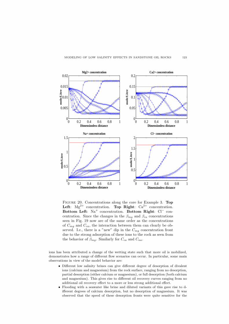
of the large adsorption of Ca2+ and Mg2+ ions on the rock surface, there exists certainregions along the core where the Ca2+ and Mg2+ concentrations are below the injectedand initial concentrations. The Na+ ions are desorbed from the rock surface and thisdesorption is responsible for the Na+ concentration profile seen in Fig. 20. The Cl− actsas a tracer and is neither desorbed or adsorbed.

7. Concluding remarks

The proposed model which couples a standard Buckley-Leverett two-phase model toa multiple ion exchange process relevant for sandstone, and where desorption of divalent


0 0.2 0.4 0.6 0.8 10

0.005

0.01

0.015

0.02


Mg2+ concentration

mo

le/L

itre

0 0.2 0.4 0.6 0.8 10

0.05

0.1

0.15

0.2


Ca2+ concentration

mo

le/L

itre

0 0.2 0.4 0.6 0.8 10

0.5

1

1.5


Na+ concentration

mo

le/L

itre

0 0.2 0.4 0.6 0.8 10

0.5

1

1.5

2


Cl− concentrationm

ole

/Litre

Figure 20. Concentrations along the core for Example 3. TopLeft: Mg2+ concentration. Top Right: Ca2+ concentration.Bottom Left: Na+ concentration. Bottom Right: Cl− con-centration. Since the changes in the βmg and βca concentrationsseen in Fig. 19 now are of the same order as the concentrationsof Cmg and Cca, the interaction between them can clearly be ob-served. I.e., there is a ”new” dip in the Cmg concentration frontdue to the strong adsorption of these ions to the rock as seen fromthe behavior of βmg. Similarly for Cca and Cna.

ions has been attributed a change of the wetting state such that more oil is mobilized,demonstrates how a range of different flow scenarios can occur. In particular, some mainobservations in view of the model behavior are:

• Different low salinity brines can give different degree of desorption of divalentions (calcium and magnesium) from the rock surface, ranging from no desorption,partial desorption (either calcium or magnesium), or full desorption (both calciumand magnesium). This gives rise to different oil recovery curves ranging from noadditional oil recovery effect to a more or less strong additional effect.

• Flooding with a seawater like brine and diluted variants of this gave rise to d-ifferent degrees of calcium desorption, but no desorption of magnesium. It wasobserved that the speed of these desorption fronts were quite sensitive for the


brine composition, leading to a range of different oil recovery behavior in theinitial stage (first 2 days) of the simulated flooding experiments.

• The model demonstrates that the oil recovery is quite sensitive to the compositionof the formation water relative to the injected water composition.

In the future we will focus on expanding the model by including effects of e.g. capaillarypressure and mineral solubility, as well as evaluating the model by carrying out systematiccomparison studies between predicted model behavior and different experimental works,as mentioned in the introduction part.

Acknowledgments

This research has been supported by the Norwegian Research Council, Statoil, DongEnergy, and GDF Suez, through the project Low Salinity Waterflooding of North SeaSandstone Reservoirs. The second author is also supported by A/S Norske Shell.

References

1. G. Ali, V. Furuholt, R. Natalini, and I. Torcicollo, A mathematical model of sulphitechemical aggression of limestones with high permeability. part i. modeling and quali-tative analysis, Transport Porous Med 69 (2007), 109–122.

2. , A mathematical model of sulphite chemical aggression of limestones with highpermeability. part ii. numerical approximation, Transport Porous Med 69 (2007), 175–188.

3. M. Alotaibi, R. Azmy, and H. Nasr-El-Din, A comprehensive EOR study using lowsalinity water in sandstone reservoirs, 17th Symposium on Improved Oil Recovery(Tulsa, Oklahoma, USA), SPE 129976, April 2010.

4. C.A.J. Appelo and D. Postma, Geochemistry, groundwater and polution, 2nd editioned., CRC Press, 2005.

5. A. Ashraf, N. Hadia, and O. Torsæter, Laboratory investigation of low salinity water-flooding as secondary recovery process: effect of wettability, SPE Oil and Gas IndiaConference and Exhibition (Mumbai, India), SPE 129012, January 2010.

6. T. Austad, A. Rezaeidoust, and T. Puntervold, Chemical mechanism of low salinitywater flooding in sandstone reservoirs, 17th Symposium on Improved Oil Recovery(Tulsa, Oklahoma, USA), SPE 129767, April 2010.

7. G.I. Barenblatt, V.M. Entov, and V.M. Ryzhik, Theory of fluid flows through naturalrocks, Kluwer Academic Publisher, 1990.

8. J. Bear, Dynamics of fluids in porous media, Elsevier, Amsterdam, 1972.9. S. Berg, A. Cense, E. Jansen, and K. Bakker, Direct experimental evidence of wet-

tability modification by low salinity, International Symposium of the Society of CoreAnalyst (Noordwijk, The Netherlands), September 2009.

10. D. Boyd and K. Al Nayadi, Validating laboratory measured archie saturation exponentsusing non-resistivity based methods, International Symposium of the Society of CoreAnalyst (Abu Dhabi, UAE), October 2004.

11. Jui-Sheng Chen and Chen-Wuing Liu, Numerical simulation of the evolution of aquiferporosity and species concentrations during reactive transport, Computers & Geo-sciences 28 (2002), no. 4, 485 – 499.

12. Z. Chen, G. Huan, and Y. Ma, Computational methods for multiphase flows in porousmedia, Computational Science And Engineering, Society for Industrial and AppliedMathematics, 2006.

13. M. Cissokho, S. Boussour, P. Cordier, H. Bertin, and G. Hamon, Low salinity oilrecovery on clayey sandstone: experimental study, International Symposium of theSociety of Core Analyst (Noordwijk, The Netherlands), September 2009.

14. S. Evje and A. Hiorth, A mathematical model for dynamic wettability alteration con-trolled by water-rock chemistry, Networks and Heterogeneous Media 5 (2010), 217–256.

15. , A model for interpretation of brine-dependent spontaneous imbibition exper-iments, Advances in Water Resources 34 (2011), 1627–1642.

REFERENCES 125

16. S. Evje, A. Hiorth, M.V. Madland, and R.Korsnes, A mathematical model relevant forweakening of chalk reservoirs due to chemical reactions, Networks and HeterogeneousMedia 4 (2009), 755–788.

17. H. Helgeson, D. Kirkham, and G. Flowers, Theoretical prediction of the thermodynam-ic behaviour of aqueous electrolytes by high pressure and temperatures; ii, AmericanJournal of Science 274 (1974), 1199–1261.

18. H. Helgeson, D. Kirkham, and G Flowers, Theoretical prediction of the thermodynamicbehaviour of aqueous electrolytes by high pressure and temperatures; iv, AmericanJournal of Science 281 (1981), 1249–1516.

19. A. Hiorth, L.M. Cathles, J. Kolnes, O. Vikane, A. Lohne, and Madland M.V., A chem-ical model for the seawater-CO2-carbonate system – aqueous and surface chemistry,Wettability Conference (Abu Dhabi, UAE), October 2008.

20. G. Hirasaki, Ion exchange with clays in the presence of surfactants, SPE J. 22 (1982),181–192.

21. P.P. Jadhunandan and N.R. Morrow, Effect of wettability on waterflood recovery forcrude oil/brine/rock systems., SPE Reservoir Engineering 12 (1995), 40–46.

22. G.R. Jerauld, C.Y. Lin, K.J. Webb, and J.C. Seccombe, Modeling low-salinity water-flooding, SPE Reservoir Evaluation & Engineering 11 (2008), 1000–1012.

23. S. Jin, Z. Xin, Shi Jin, and Zhouping Xin, The relaxation schemes for systems ofconservation laws in arbitrary space dimensions, Comm. Pure Appl. Math 48 (1995),235–277.

24. A. Lager, K. Webb, C. Black, M. Singleton, and K. Sorbie, Low salinity oil recov-ery: An experimental investigation, International Symposium of the Society of CoreAnalyst (Trondhiem, Norway), September 2006.

25. A.C. Lasaga, Kinetic theory in the earth sciences, Princeton series in geochemistry,Princeton University Press, 1998.

26. D.A. Nield and A. Bejan, Convection in porous media, Springer, 2006.27. E.H. Oelkers and J. Schott, Thermodynamics and kinetics of water-rock interaction,

Reviews in Mineralogy and Geochemistry, no. v. 70, Mineralogical Society of America,2009.

28. A. Omekeh, S. Evje, I. Fjelde, and H.A. Friis, Experimental and modeling investigationof ion exchange during low salinity waterflooding, International Symposium of theSociety of Core Analyst (Austin, Texas, USA), September 2011.

29. Adolfo P. Pires, Pavel G. Bedrikovetsky, and Alexander A. Shapiro, A splitting tech-nique for analytical modelling of two-phase multicomponent flow in porous media,Journal of Petroleum Science and Engineering 51 (2006), no. 1 - 2, 54 – 67.

30. G.A. Pope, L.W. Lake, and F.G. Helfferich, Cation exchange in chemical flooding:Part 1–basic theory without dispersion, Society of Petroleum Engineers Journal 18(1978), 418–434.

31. H. Pu, X. Xie, P. Yin, and N. Morrow, Application of coalbed methane water to oilrecovery by low salinity waterflooding, SPE Improved Oil Recovery Symposium (Tulsa,Oklahoma, USA), SPE 113410, April 2008.

32. M. Sahimi, Flow and transport in porous media and fractured rock: From classicalmethods to modern approaches, John Wiley & Sons, 2011.

33. S.Boussour, M. Cissokho, P. Cordier, H. Bertin, and G. Hamon, Oil recovery by lowsalinity brine injection: laboratory results outcrop and reservoir cores, SPE AnnualTechnical Conference and Exhibition (New Orleans, USA), SPE 124277, October 2009.

34. J. Seccombe, A. Lager, K. Webb, G. Jerauld, and E. Fueg, Improving waterflood re-covery: LoSal EOR field evaluation, SPE/DOE Symposium on Improved Oil Recovery(Tulsa, Oklahoma, USA), SPE 113480, April 2008.

35. M. Sharma and P. Filoco, Effect of brine salinity and crude oil properties on oilrecovery and residual saturations, SPE Journal 5 (2000), 293–300.

36. K. Skrettingland, K. Holt, M. Tweheyo, and I. Skjevrak, Snorre low salinity water in-jection - core flooding experiments and single well field pilot, Symposium on ImprovedOil Recovery (Tulsa, Oklahoma, USA), SPE 129877, April 2010.

126 REFERENCES

37. Skule Strand, Eli J. Hagnesen, and Tor Austad, Wettability alteration of carbonates-effects of potential determining ions (Ca2+ and SO2−

4 ) and temperature, Colloids andSurfaces A: Physicochemical and Engineering Aspects 275 (2006), no. 1-3, 1 – 10.

38. T.A.Dutra, A.P.Pires, and P.G.Bedrikovetsky, A new splitting scheme and existenceof elliptic region for gasflood modeling, SPE J. 14 (2009), no. 1, 101–111.

39. G. Tang and N. Morrow, Oil recovery by waterflooding and imbibition - invading brinecation valency and salinity, International Symposium of the Society of Core Analysts(Golden, CO), August 1999.

40. Guo Qing Tang and Norman R Morrow, Influence of brine composition and finesmigration on crude oil/brine/rock interactions and oil recovery, Journal of PetroleumScience and Engineering 24 (1999), no. 2-4, 99 – 111.

41. I. Tripathi and K.K. Mohanty, Instability due to wettability alteration in displacementsthrough porous media, Chemical Engineering Science 63 (2008), no. 21, 5366 – 5374.

42. K. Webb, C. Black, and H. Al-Jeel, Low salinity oil recovery - log inject log, SPE/DOESymposium on Improved Oil Recovery (Tulsa, Oklahoma, USA), SPE 89379, April2004.

43. K. Webb, A. Lager, and C. Black, Comparison of high/low salinity water/oil relativepermeability, International Symposium of the Society of Core Analysts (Abu Dhabi,UAE), November 2008.

44. Hasan O. Yildiz and Norman R. Morrow, Effect of brine composition on recovery ofmoutray crude oil by waterflooding, Journal of Petroleum Science and Engineering 14

(1996), no. 3-4, 159 – 168.45. L. Yu, S. Evje, H. Kleppe, T. Kaarstad, I. Fjelde, and S.M. Skjaeveland, Modelling

of wettability alteration processes in carbonate oil reservoirs, Networks and Heteroge-neous Media 3 (2008), 149–183.

46. , Spontaneous imbibition of seawater into preferentially oil-wet chalk cores : Ex-periments and simulations, Journal of Petroleum Science and Engineering 66 (2009),no. 3-4, 171 – 179.

47. W. Yu-shu and B. Baojun, Efficient simulstion for low salinity waterflooding in porousand fractured reservoirs, SPE Reservoir Simulation Symposium (The Woodlands,Texas, USA), SPE 118830, February 2009.

48. Y. Zhang and N. Morrow, Comparison of secondary and tertiary recovery with changein injection brine composition for crude oil/sandstone combinations, SPE/DOE Sym-posium on Improved Oil Recovery (Tulsa, Oklahoma, USA), SPE 99757, April 2006.

8. APPENDIX A: DATA FOR WATER-ROCK CHEMISTRY

Activity coefficients. Along the line of the previous work [16] the following values,taken from [4], are used for the constants a0

i :

a0ca = 5, a0

na = 4, a0cl = 3.5, a0

mg = 5.5, a0so = 5.(94)

and for b0i we use:

b0ca = 0.165, b0na = 0.075, b0cl = 0.015, b0mg = 0.2, b0so = −0.04.(95)

Moreover, we shall use the following values for A(T ) and B(T ) taken from [18, 17]:

(96) A(T = 80) = 0.5706, B(T = 80) = 0.3381.

Core properties. The following core properties are assumed for the model examplestudied below.

• Length: L = 0.04m• Porosity: φ = 0.274• Mass of clay: Mc = 0.088Kg/Litre of core• Permeability: κ = 500mD = 500 · 0.987 · 10−15 m2.

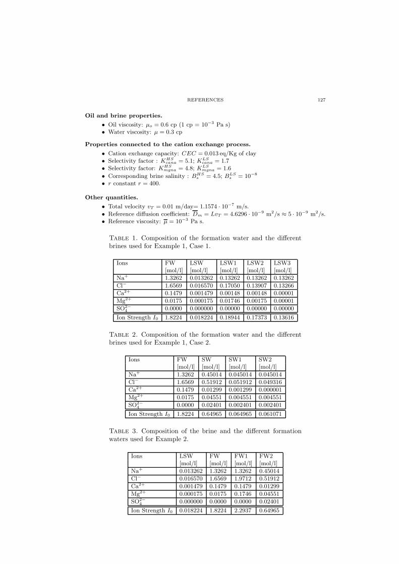
REFERENCES 127

Oil and brine properties.

• Oil viscosity: µo = 0.6 cp (1 cp = 10−3 Pa s)• Water viscosity: µ = 0.3 cp

Properties connected to the cation exchange process.

• Cation exchange capacity: CEC = 0.013 eq/Kg of clay• Selectivity factor : KHS

cana = 5.1; KLScana = 1.7

• Selectivity factor: KHSmgna = 4.8; KLS

mgna = 1.6

• Corresponding brine salinity : BHSs = 4.5; BLS

s = 10−8

• r constant r = 400.

Other quantities.

• Total velocity vT = 0.01 m/day= 1.1574 · 10−7 m/s.

• Reference diffusion coefficient: Dm = LvT = 4.6296 · 10−9 m2/s ≈ 5 · 10−9 m2/s.• Reference viscosity: µ = 10−3 Pa s.

Table 1. Composition of the formation water and the differentbrines used for Example 1, Case 1.

Ions FW LSW LSW1 LSW2 LSW3[mol/l] [mol/l] [mol/l] [mol/l] [mol/l]

Na+ 1.3262 0.013262 0.13262 0.13262 0.13262

Cl− 1.6569 0.016570 0.17050 0.13907 0.13266

Ca2+ 0.1479 0.001479 0.00148 0.00148 0.00001

Mg2+ 0.0175 0.000175 0.01746 0.00175 0.00001

SO2−4 0.0000 0.000000 0.00000 0.00000 0.00000

Ion Strength I0 1.8224 0.018224 0.18944 0.17373 0.13616

Table 2. Composition of the formation water and the differentbrines used for Example 1, Case 2.

Ions FW SW SW1 SW2[mol/l] [mol/l] [mol/l] [mol/l]

Na+ 1.3262 0.45014 0.045014 0.045014

Cl− 1.6569 0.51912 0.051912 0.049316

Ca2+ 0.1479 0.01299 0.001299 0.000001

Mg2+ 0.0175 0.04551 0.004551 0.004551

SO2−4 0.0000 0.02401 0.002401 0.002401

Ion Strength I0 1.8224 0.64965 0.064965 0.061071

Table 3. Composition of the brine and the different formationwaters used for Example 2.

Ions LSW FW FW1 FW2[mol/l] [mol/l] [mol/l] [mol/l]

Na+ 0.013262 1.3262 1.3262 0.45014

Cl− 0.016570 1.6569 1.9712 0.51912

Ca2+ 0.001479 0.1479 0.1479 0.01299

Mg2+ 0.000175 0.0175 0.1746 0.04551

SO2−4 0.000000 0.0000 0.0000 0.02401

Ion Strength I0 0.018224 1.8224 2.2937 0.64965

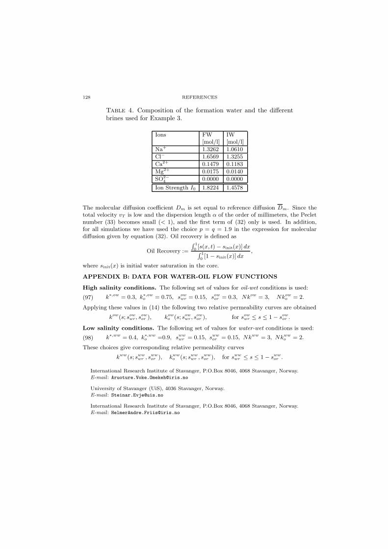
128 REFERENCES

Table 4. Composition of the formation water and the differentbrines used for Example 3.

Ions FW IW[mol/l] [mol/l]

Na+ 1.3262 1.0610

Cl− 1.6569 1.3255

Ca2+ 0.1479 0.1183

Mg2+ 0.0175 0.0140

SO2−4 0.0000 0.0000

Ion Strength I0 1.8224 1.4578

The molecular diffusion coefficient Dm is set equal to reference diffusion Dm. Since thetotal velocity vT is low and the dispersion length α of the order of millimeters, the Pecletnumber (33) becomes small (< 1), and the first term of (32) only is used. In addition,for all simulations we have used the choice p = q = 1.9 in the expression for moleculardiffusion given by equation (32). Oil recovery is defined as

Oil Recovery :=

∫ 1

0[s(x, t)− sinit(x)] dx∫ 1

0[1− sinit(x)]dx

,

where sinit(x) is initial water saturation in the core.

APPENDIX B: DATA FOR WATER-OIL FLOW FUNCTIONS

High salinity conditions. The following set of values for oil-wet conditions is used:

k∗,ow = 0.3, k∗,owo = 0.75, sowwr = 0.15, sowor = 0.3, Nkow = 3, Nkow

o = 2.(97)

Applying these values in (14) the following two relative permeability curves are obtained

kow(s; sowwr, sowor ), kow

o (s; sowwr, sowor ), for sowwr ≤ s ≤ 1− sowor .

Low salinity conditions. The following set of values for water-wet conditions is used:

k∗,ww = 0.4, k∗,wwo =0.9, sww

wr = 0.15, swwor = 0.15, Nkww = 3, Nkww

o = 2.(98)

These choices give corresponding relative permeability curves

kww(s; swwwr , s

wwor ), kww

o (s; swwwr , s

wwor ), for sww

wr ≤ s ≤ 1− swwor .

International Research Institute of Stavanger, P.O.Box 8046, 4068 Stavanger, Norway.E-mail : [email protected]

University of Stavanger (UiS), 4036 Stavanger, Norway.E-mail : [email protected]

International Research Institute of Stavanger, P.O.Box 8046, 4068 Stavanger, Norway.E-mail : [email protected]

Modeling of Low Salinity Effects

Documents

Transcript of Modeling of Low Salinity Effects