MODELING OF INTERIOR BEAM-COLUMN JOINTS FOR · PDF fileii Modeling of Interior Beam-Column...
177
MODELING OF INTERIOR BEAM-COLUMN JOINTS FOR NONLINEAR ANALYSIS OF REINFORCED CONCRETE FRAMES by Zhangcheng Pan A thesis submitted in conformity with the requirements for the degree of Master of Applied Science Graduate Department of Civil Engineering University of Toronto © Copyright by Zhangcheng Pan (2016)
Transcript of MODELING OF INTERIOR BEAM-COLUMN JOINTS FOR · PDF fileii Modeling of Interior Beam-Column...

MODELING OF INTERIOR BEAM-COLUMN JOINTS FOR
NONLINEAR ANALYSIS OF REINFORCED CONCRETE FRAMES
by
Zhangcheng Pan
A thesis submitted in conformity with the requirements
for the degree of Master of Applied Science
Graduate Department of Civil Engineering
University of Toronto
© Copyright by Zhangcheng Pan (2016)

ii
Modeling of Interior Beam-Column Joints for Nonlinear Analysis of
Reinforced Concrete Frames
Zhangcheng Pan
Master of Applied Science
Graduate Department of Civil Engineering
University of Toronto
2016
ABSTRACT
Beam-column connections are often assumed rigid in traditional frame analysis, yet they undergo
significant shear deformations and greatly contribute to story drifts during earthquake loading.
Although local joint models are available in the literature for the investigation of single, isolated
joints, there is a lack of holistic frame analysis procedures simulating the joint behavior in
addition to important global failure modes such as beam shear, column shear, column axial, and
soft story failures. The objective of this study is to capture the impact of local joint deformations
on the global frame response in a holistic analysis by implementing a joint model into a
previously-developed global frame analysis procedure. The implemented joint element simulates
joint shear deformations and bar-slip effects. Concrete confinement effects are also considered so
that both older and new joints can be modeled. The developed procedure provides better overall
load-deflection response predictions including the local joint response.

iii
TABLE OF CONTENTS
ABSTRACT .................................................................................................................................... ii
TABLE OF CONTENTS ............................................................................................................... iii
LIST OF TABLES .......................................................................................................................... v
LIST OF FIGURES ...................................................................................................................... vii
CHAPTER 1: INTRODUCTION ................................................................................................... 1
1.1 Motivations for the Study ...................................................................................................... 1
1.2 Nonlinear Frame Analysis Program, VecTor5 ...................................................................... 3
1.3 Objectives of the Study ......................................................................................................... 5
1.4 Thesis Organization............................................................................................................... 6
CHAPTER 2: MODELING OF BEAM-COLUMN JOINTS ........................................................ 8
2.1 Chapter Layout ...................................................................................................................... 8
2.2 Beam-Column Joint Behavior ............................................................................................... 8
2.3 Review of Existing Behavior Models for Beam-Column Joints ......................................... 12
2.3.1 The Modified Compression Field Theory .................................................................... 13
2.3.2 The Strut-and-Tie Model .............................................................................................. 19
2.3.3 Bond Stress-Slip Relationship ...................................................................................... 22
2.4 Review of Existing Beam-Column Joint Models ................................................................ 28
2.4.1 Rotational Hinge Models .............................................................................................. 28
2.4.2 Component Models....................................................................................................... 30
CHAPTER 3: IMPLEMENTED JOINT ELEMENT MODEL.................................................... 36
3.1 Chapter Layout .................................................................................................................... 36
3.2 Joint Element Formulation .................................................................................................. 36
3.3 Modeling Bond Slip Response ............................................................................................ 41
3.4 Modeling Joint Shear Response .......................................................................................... 46
3.5 Modeling of Interface Shear Response ............................................................................... 49
3.6 Computation Schemes ......................................................................................................... 50
CHAPTER 4: JOINT IMPLEMENTATION IN VECTOR5 ....................................................... 52
4.1 Chapter Layout .................................................................................................................... 52
4.2 Global Frame Modeling ...................................................................................................... 52

iv
4.3 Joint Analysis Algorithm .................................................................................................... 57
4.3.1 Subroutine: Local Joint Element .................................................................................. 57
4.3.2 Subroutine: Bar Slip Spring .......................................................................................... 68
4.3.3 Subroutine: Shear Panel ................................................................................................ 70
4.4 Modifications of the Global Frame Analysis Procedure ..................................................... 75
4.4.1 Detection of Interior Joints ........................................................................................... 75
4.4.2 Assembly of the Global Stiffness Matrix ..................................................................... 76
4.4.3 Solution to the Global Frame Analysis......................................................................... 77
4.5 Guidelines for Modeling Beam-Column Joints .................................................................. 78
4.6 Interpretation of Results ...................................................................................................... 79
4.6.1 Output Files .................................................................................................................. 79
4.6.2 Graphical Representation ............................................................................................. 81
CHAPTER 5: MODEL EVALUATION AND VERIFICATION ............................................... 83
5.1 Chapter Layout .................................................................................................................... 83
5.2 Beam-Column Subassemblies ............................................................................................. 83
5.2.1 Summary ....................................................................................................................... 83
5.2.2 Shiohara and Kusuhara (2007) ..................................................................................... 87
5.2.3 Park and Dai (1988) ...................................................................................................... 98
5.2.4 Noguchi and Kashiwazaki (1992) .............................................................................. 109
5.2.5 Attaalla and Agbabian (2004)..................................................................................... 119
5.3 Parametric Study for Beam-Column Subassemblies ........................................................ 132
5.4 Frame Structures ............................................................................................................... 138
5.4.1 Summary ..................................................................................................................... 138
5.4.2 Xue et al. Frame (2011) .............................................................................................. 138
5.4.3 Ghannoum and Moehle (2012) ................................................................................... 144
5.4.4 Pampanin et al. (2007) ................................................................................................ 150
CHAPTER 6: SUMMARY, CONCLUSIONS AND RECOMMEDATIONS .......................... 157
6.1 Summary ........................................................................................................................... 157
6.2 Conclusions ....................................................................................................................... 157
6.3 Recommendations for Future Research ............................................................................ 159
REFERENCES ........................................................................................................................... 161

v
LIST OF TABLES
Table 3.1: Average bond stress for various rebar conditions ....................................................... 44
Table 4.1: List of input variables required by local joint element subroutine ............................. 60
Table 4.2: Iterations to convergence for selected stiffness values ............................................... 64
Table 5.1: Material behavior models and analysis parameters used in VecTor5 ......................... 84
Table 5.2: Summary of the specimen properties and analytical results of interior beam-column
subassemblies ................................................................................................................................ 85
Table 5.3: Material properties of Specimens A1 and D1 ............................................................. 88
Table 5.4: General material specifications of Specimen A1 ........................................................ 91
Table 5.5: Reinforced concrete material specifications of Specimen A1 .................................... 91
Table 5.6: Longitudinal reinforcement material specifications of Specimen A1 ........................ 92
Table 5.7: Comparison of experimental and analytical results of Specimen A1 ......................... 92
Table 5.8: Stress in the longitudinal bars at the joint panel interface of Specimen A1 ............... 96
Table 5.9: Comparison of experimental and analytical results of Specimen D1 ......................... 97
Table 5.10: Material properties of Specimens Unit 1 and Unit 2 .............................................. 101
Table 5.11: General material specifications of Specimen Unit 1 ............................................... 103
Table 5.12: Reinforced concrete material specifications of Specimen Unit 1 ........................... 103
Table 5.13: Longitudinal reinforcement material specifications of Specimen Unit 1 ............... 104
Table 5.14: Comparison of experimental and analytical results of Specimen Unit 1 ................ 105
Table 5.15: Stress in the longitudinal bars at the joint panel interface of Specimen Unit 1 ...... 107
Table 5.16: Comparison of experimental and analytical results of Specimen Unit 2 ................ 108
Table 5.17: Material properties of Specimens OKJ2 and OKJ6 ................................................ 110
Table 5.18: General material specifications of Specimen OKJ2 ............................................... 113
Table 5.19: Reinforced concrete material specifications of Specimen OKJ2 ............................ 113
Table 5.20: Longitudinal reinforcement material specifications of Specimen OKJ2 ................ 114
Table 5.21: Comparison of experimental and analytical results of Specimen OKJ2 ................. 114
Table 5.22: Stress in the longitudinal bars at the joint panel interface of Specimen OKJ2 ....... 117
Table 5.23: Comparison of experimental and analytical results of Specimen OKJ6 ................. 118
Table 5.24: Material properties of Specimens SHC1, SHC2 and SOC3 ................................... 121

vi
Table 5.25: General material specifications of Specimen SHC1 ............................................... 123
Table 5.26: Reinforced concrete material specifications of Specimen SHC1 ........................... 123
Table 5.27: Longitudinal reinforcement material specifications of Specimen SHC1................ 123
Table 5.28: Comparison of experimental and analytical results of Specimen SHC1 ................ 124
Table 5.29: Stress in the longitudinal bars at the joint panel interface of Specimen SHC1 ...... 126
Table 5.30: Comparison of experimental and analytical results of Specimen SHC2 ................ 126
Table 5.31: Comparison of experimental and analytical results of Specimen SOC3 ................ 129
Table 5.32: Material properties of Specimen HPCF-1 ............................................................... 140
Table 5.33: Comparison of experimental and analytical results of Specimen HPCF-1 ............. 143
Table 5.34: Material properties of Ghannoum and Moehle Frame ............................................ 145
Table 5.35: Material properties of Pampanin et al. Frame ......................................................... 152

vii
LIST OF FIGURES
Figure 1.1: Common failure modes of frames subjected to seismic loading (Google Images) ..... 1
Figure 1.2: Contributions of displacement factors to story drift for an older type joint, Specimen
CD15-14, subjected to reversed cyclic loading (Walker, 2001) ..................................................... 3
Figure 1.3: Experimental and analytical load-displacement responses of Specimen SHC2 tested
by Attaalla and Agbabian (2004) .................................................................................................... 5
Figure 2.1: Three types of beam-column connections in a reinforced concrete frame (Kim and
LaFave, 2009) ................................................................................................................................. 9
Figure 2.2: Forces expected to develop at the perimeter of an interior joint in a frame under
seismic actions (Mitra, 2007) ........................................................................................................ 10
Figure 2.3: Load distribution at the joint region (Hakuto et al., 1999) ........................................ 10
Figure 2.4: Major shear resisting mechanisms: (a) the concrete strut mechanism and (b) the truss
mechanism (Pauley et al., 1978) ................................................................................................... 11
Figure 2.5: Deformed reinforced concrete joint with bond slip and bar pullout (Altoontash, 2004)
....................................................................................................................................................... 12
Figure 2.6: Reinforced concrete element subjected to normal and shear stresses (Vecchio and
Collins, 1986) ................................................................................................................................ 13
Figure 2.7: Stress-strain relationship for concrete under (a) uniaxial compression and (b)
uniaxial tension (Vecchio and Collins, 1986) ............................................................................... 15
Figure 2.8: B Regions and D Regions in a reinforced concrete frame structure (Schlaich et al.,
1987) ............................................................................................................................................. 19
Figure 2.9: The strut-and-tie model: (a) single-strut model, (b) distributed-truss model, (c)
combined strut-truss model, and (d) definition of the strut width in combined strut-truss
mechanism (Mitra, 2007) .............................................................................................................. 21
Figure 2.10: Test setup in the bond experiment conducted by Viwathanatepa et al. (1979): (a)
the elevation view of the specimen and (b) the testing apparatus ................................................ 23
Figure 2.11: Formulation of bond model proposed by Viwathanatepa et al. (1979): (a)
monotonic skeleton bond stress-slip Curve, (b) finite soft layer elements, and (c) load-
displacement relationship of a #8 (25M) bar ................................................................................ 24
Figure 2.12: Proposed analytical model for local bond stress-slip relationship for confined
concrete subjected to monotonic and cyclic loading. (Eligenhausen et al., 1983) ....................... 26
Figure 2.13: Monotonic envelope curve of bar stress versus loaded-end slip relationship (Zhao
and Sritharan, 2007) ...................................................................................................................... 27
viii
Figure 2.14: Joint model proposed by Alath and Kunnath (Alath and Kunnath, 1995; figure
adopted from Celik and Ellingwood, 2008) .................................................................................. 28
Figure 2.15: Joint model proposed by Altoontash (Altoontash, 2004) ........................................ 29
Figure 2.16: Joint model proposed by Shin and LaFave (Shin and LaFave, 2004) ..................... 30
Figure 2.17: Joint model proposed by Lowes and Altoontash (Lowes and Altoontash, 2003) ... 31
Figure 2.18: Joint model proposed by Ghobarah and Youssef (Ghobarah and Youssef, 2001) .. 32
Figure 2.19: Joint model proposed by Fleury et al. (Fleury et al., 2000)..................................... 33
Figure 2.20: Joint model proposed by Elmorsi et al.: (a) proposed element and (b) details of the
bond slip element (Elmorsi et al., 2000) ....................................................................................... 34
Figure 2.21: Joint model proposed by Shiohara (Shiohara, 2004)............................................... 35
Figure 3.1: Implemented interior beam-column joint model (Mitra and Lowes, 2007) .............. 37
Figure 3.2: Definition of displacements, deformations and forces in the model: (a) external
displacements and component deformations and (b) external forces and component forces ....... 38
Figure 3.3: Compatibility equations of the implemented joint model (Mitra and Lowes, 2007) 40
Figure 3.4: Bond stress and bar stress distribution along a reinforcing bar anchored in a joint .. 43
Figure 3.5: Bar stress versus slip relationship from various studies and experiments ................. 44
Figure 3.6: Sectional analysis of a frame member at the nominal flexural strength: (a) member
cross-section, (b) strain distribution, (c) stress distribution, and (d) forces on the member ........ 46
Figure 3.7: Idealized diagonal concrete compression strut model ............................................... 47
Figure 3.8: Reduction equations to the concrete compression strength (Mitra and Lowes, 2007)
....................................................................................................................................................... 48
Figure 3.9: Envelope of the shear stress versus slip response for the interface shear springs
(Lowes and Altoontash, 2003) ...................................................................................................... 49
Figure 4.1: Typical frame model in VecTor5 .............................................................................. 54
Figure 4.2: Longitudinal and shear strain distributions across sectional depth for a layered
analysis (Guner and Vecchio, 2010) ............................................................................................. 55
Figure 4.3: Flowchart for the global frame analysis of VecTor5 (Guner and Vecchio, 2010) .... 55
Figure 4.4: Joint element implementation in VecTor5 ................................................................ 56
Figure 4.5: Flowchart of solution process for the joint element .................................................. 59
Figure 4.6: Load-displacement response of interface shear spring with different stiffness ........ 64
Figure 4.7: Partitioned joint element stiffness matrix .................................................................. 66
Figure 4.8: Joint analysis matrix for frames with multiple interior joints ................................... 67
Figure 4.9 Joint panel displacements and rotations ..................................................................... 67

ix
Figure 4.10: Flowchart of the solution process for the bar slip springs ....................................... 68
Figure 4.11: Modified bar stress versus slip relationship ............................................................ 69
Figure 4.12: Flowchart of solution process for the shear panel ................................................... 70
Figure 4.13: Stress-strain model for monotonic loading of confined and unconfined concrete
(Mander et al., 1988) ..................................................................................................................... 71
Figure 4.14: Effectively confined concrete for rectangular tie reinforcement (Mander et al., 1988)
....................................................................................................................................................... 72
Figure 4.15: Interior joint information in the common blocks .................................................... 76
Figure 4.16: Assembling the global stiffness matrix: (a) stiffness of members, (b) stiffness of
joints, and (c) stiffness of the structure ......................................................................................... 77
Figure 4.17: Layout of member analysis results for members in joint regions ........................... 79
Figure 4.18: Layout of interior joint analysis results in the output files ...................................... 80
Figure 4.19: Definition of layers and faces in joint analysis results ............................................ 81
Figure 4.20: Sample sketch of a deformed interior joint ............................................................. 82
Figure 5.1: Test setup of Specimens A1 and D1 (adapted from Guner, 2008) ............................ 88
Figure 5.2: Sectional details of Specimens A1 and D1 ................................................................ 89
Figure 5.3: Analytical model showing dimensions, loading and support restraints of Specimens
A1 and D1 ..................................................................................................................................... 90
Figure 5.4: Analytical model showing material types of Specimens A1 and D1 ........................ 91
Figure 5.5: Comparison of the load-displacement response of Specimen A1 ............................. 93
Figure 5.6: Cracking pattern of Specimen A1: (a) observed (Shiohara and Kusuhara, 2007) and
(b) original VecTor5 simulation ................................................................................................... 94
Figure 5.7: Load versus joint shear strain relationship of Specimen A1 ..................................... 95
Figure 5.8: Comparison of the load-displacement response of Specimen D1 ............................. 96
Figure 5.9: Cracking pattern of Specimen D1: (a) observed (Shiohara and Kusuhara, 2008) and
(b) original VecTor5 simulation ................................................................................................... 98
Figure 5.10: Test setup of Specimens Unit 1 (Park and Dai, 1988) ............................................ 99
Figure 5.11: Test setup of Specimens Unit 2 (Park and Dai, 1988) .......................................... 100
Figure 5.12: Sectional details of Specimens Unit 1 and Unit 2 (Park and Dai, 1988) ............... 100
Figure 5.13: Analytical model showing dimensions, loading and support restraints of Specimens
Unit 1 and Unit 2......................................................................................................................... 102
Figure 5.14: Analytical model showing material types of Specimens Unit 1 and Unit 2 .......... 103
Figure 5.15: Comparison of the load-displacement response of Specimen Unit 1 .................... 105
x
Figure 5.16: Cracking pattern of Specimen Unit 1: (a) observed (Park and Dai, 1988) and (b)
original VecTor5 simulation ....................................................................................................... 107
Figure 5.17: Comparison of the load-displacement response of Specimen Unit 2 .................... 108
Figure 5.18: Cracking pattern of Specimen Unit 2 predicted by original VecTor5 simulation . 109
Figure 5.19: Test setup of Specimens OKJ2 and OKJ6 (Noguchi and Kashiwazaki, 1992) ..... 111
Figure 5.20: Sectional details of Specimens OKJ2 and OKJ6: (a) beam section, (b) column
section, and (c) detailed joint reinforcement (Noguchi and Kashiwazaki, 1992) ....................... 111
Figure 5.21: Analytical model showing dimensions, loading and support restraints of Specimens
OKJ2 and OKJ6 .......................................................................................................................... 112
Figure 5.22: Analytical model showing material types of Specimens OKJ2 and OKJ6 ........... 113
Figure 5.23: Comparison of the load-displacement response of Specimen OKJ2 ..................... 115
Figure 5.24: Cracking pattern of Specimen OKJ1 (Noguchi and Kashiwazaki, 1992) ............. 116
Figure 5.25: Cracking pattern of Specimen OKJ2 predicted by original VecTor5 simulation . 117
Figure 5.27: Comparison of the load-displacement response of Specimen OKJ6 ..................... 118
Figure 5.28: Cracking pattern of Specimen OKJ6 predicted by original VecTor5 simulation . 119
Figure 5.29: Test setup of Specimens SHC1, SHC2 and SOC3 (Attaalla and Agbabian, 2004)
..................................................................................................................................................... 120
Figure 5.30: Sectional details of Specimens SHC1, SHC2 and SOC3: (a) beam section, (b)
column section (Attaalla and Agbabian, 2004), and (c) detailed joint reinforcement (Attaalla,
1997) ........................................................................................................................................... 121
Figure 5.31: Analytical model showing dimensions, loading and support restraints of Specimens
SHC1, SHC2 and SOC3 ............................................................................................................. 122
Figure 5.32: Analytical model showing material types of Specimens SHC1, SHC2 and SOC3
..................................................................................................................................................... 122
Figure 5.33: Comparison of the load-displacement response of Specimen SHC1 .................... 124
Figure 5.34: Cracking pattern of Specimen SHC1: (a) observed (Attaalla and Agbabian, 2004)
and (b) original VecTor5 simulation .......................................................................................... 126
Figure 5.35: Comparison of the load-displacement response of Specimen SHC2 .................... 127
Figure 5.36: Cracking pattern of Specimen SHC2: (a) observed (Attaalla and Agbabian, 2004)
and (b) original VecTor5 simulation .......................................................................................... 128
Figure 5.37: Comparison of the load-displacement response of Specimen SOC3 .................... 129
Figure 5.38: Cracking pattern of Specimen SOC3: (a) observed (Attaalla and Agbabian, 2004)
and (b) VecTor5 simulation ........................................................................................................ 131

xi
Figure 5.39: Envelopes of the load versus the panel shear strain relationships for: (a) Specimen
SHC1, (b) Specimen SHC2, and (c) Specimen SOC3................................................................ 131
Figure 5.40: Story shear force versus story drift relationships of Specimen OKJ2 (Noguchi and
Kashiwazaki, 1992) subjected to: (a) monotonic and (b) reversed cyclic loading conditions ... 132
Figure 5.41: Comparison of the VecTor5 load-displacement responses of Specimen A1 ........ 133
Figure 5.42: Comparison of the load-displacement responses with different confinement
effectiveness coefficients ............................................................................................................ 134
Figure 5.43: Comparison of the load-displacement responses without the compression softening
effect ........................................................................................................................................... 135
Figure 5.44: Comparison of the load-displacement responses with bond stresses proposed by
Sezen and Moehle (2003) ........................................................................................................... 137
Figure 5.45: Structural details of Specimen HPCF-1 (Xue et al., 2011) ................................... 139
Figure 5.46: Applied loads on Specimen HPCF-1 (Xue et al., 2011)........................................ 140
Figure 5.47: Analytical model showing loading and support restraints of Specimens HPCF-1 141
Figure 5.48: Comparison of base shear versus roof drift response of Specimen HPCF-1 ........ 142
Figure 5.49: Failures of Specimen HPCF-1 (Xue et al., 2011) .................................................. 143
Figure 5.50: Deformed shape and cracking pattern of Specimen HPCF-1 ................................ 144
Figure 5.51: Structural details of Ghannoum and Moehle Frame (Ghannoum and Moehle, 2012)
..................................................................................................................................................... 145
Figure 5.52: Applied loads on Ghannoum and Moehle Frame (Ghannoum and Moehle, 2012)
..................................................................................................................................................... 146
Figure 5.53: Analytical model showing dimensions, loading and support restraints of Ghannoum
and Moehle Frame ...................................................................................................................... 147
Figure 5.54: Comparison of base shear versus first floor drift response of Ghannoum and
Moehle Frame ............................................................................................................................. 148
Figure 5.55: Failures of Ghannoum and Moehle Frame (Ghannoum and Moehle, 2012) ........ 149
Figure 5.56: Damage of interior joints in Ghannoum and Moehle Frame (Ghannoum and Moehle,
2012) ........................................................................................................................................... 149
Figure 5.57: Deformed shape and cracking pattern of Ghannoum and Moehle Frame ............. 150
Figure 5.58: Structural details of Pampanin et al. Frame (Pampanin et al., 2007) .................... 151
Figure 5.59: Applied Loads on Pampanin et al. Frame (Pampanin et al., 2007) ....................... 152
Figure 5.60: Analytical model showing dimensions, loading and support restraints of Pampanin
et al. Frame.................................................................................................................................. 153
Figure 5.61: Comparison of base shear versus top drift response of Pampanin et al. Frame .... 154

xii
Figure 5.62: Failures of Pampanin et al. Frame (Pampanin et al., 2003) .................................. 155
Figure 5.63: Damage of interior joints in Pampanin et al. Frame (Pampanin et al., 2007) ....... 155
Figure 5.64: Deformed shape and cracking pattern of Pampanin et al. Frame .......................... 156

1
CHAPTER 1
INTRODUCTION
1.1 Motivations for the Study
According to the U.S. Geological Survey, at least 850,000 people were killed and more than 3
million buildings collapsed or were damaged during the 26 major earthquake events that
occurred over the past two decades. Reinforced concrete frame structures were common among
those buildings. Common failure modes observed after earthquakes included beam-column joint
shear, column shear, beam shear, column axial, reinforcement bond slip, foundation failures and
soft story failures, as illustrated in Figure 1.1.
Figure 1.1: Common failure modes of frames subjected to seismic loading (Google Images)
Although the joint shear failure is a local failure mechanism, it often leads to progressive
collapse of buildings. Insufficient anchorage lengths of reinforcing bars, unconfined connections,
and deterioration of reinforced concrete materials are the main contributors to this type of failure.
Joint Shear Failure
Column Axial Failure
Beam Shear Failure
Column Shear Failure Soft Story Failure

2
Frame joints designed prior to the 1970’s according to older design standards, with little or no
transverse reinforcement, exhibit non-ductile response and are more vulnerable to joint shear
failures. Older design codes did not specify a limit on the joint shear stress or required joint
transverse reinforcement prior to the pioneering experiment of Hanson and Connor (1967). As a
result, joints in these frames exhibit relatively high joint shear, which contributes to greater story
drifts, and higher bond stresses, which may cause bar slippage under seismic loading.
Proper reinforcement detailing in beam-column joints is still a subject of active research. Joints
in newer buildings possess better reinforcement detailing with transverse reinforcement as
specified in the concrete building design codes such as CSA A23.3-14. Nonetheless,
experimental tests have demonstrated that the newer joint types will still exhibit shear cracking
under a strong seismic loading, significantly contributing to story drifts of the global structure
(Shin and LaFave, 2004).
In the traditional analysis of reinforced concrete frame structures subjected to seismic loading,
beam-column joints are assumed rigid. This assumption implies that the joint core remains
elastic and deforms as a rigid body throughout an earthquake even if the beams and columns
undergo significant deformation and sustain severe damage. On the contrary, experimental
studies (e.g., Walker, 2001) have demonstrated that beam-column joint deformations due to
shear cracking and bond slip are major contributors to lateral story drifts. One extreme case
example including a non-ductile beam-column joint containing no transverse reinforcement is
presented in Figure 1.2. Since the pioneering experiment in 1967, there has been an ongoing
effort in understanding the behavior of beam-column joints under seismic actions, and creating
numerical simulation methods to model and determine joint response under various loading
conditions. Researchers have proposed a variety of beam-column joint models. These models can
be categorized into three classes: rotational hinge models, component models, and finite element
models. Each model has its advantages and limitations, and there is no scientific consensus on a
model that is optimal for all applications.

3
Figure 1.2: Contributions of displacement factors to story drift for an older type joint, Specimen
CD15-14, subjected to reversed cyclic loading (Walker, 2001)
In spite of the developments in understanding and quantifying joint behavior, there is a lack of
holistic frame analysis procedures simulating the joint behavior in addition to other important
global failure modes. One commonly used technique to model joints in frame analysis
procedures is known as “semi-rigid end offsets”. Although this approach is employed to account
for increased strengths in joint cores by increasing the stiffness of the joints, it may lead to
overestimation of joint strength, joint stiffness and energy dissipation, as well as an
underestimation of lateral story drifts. These inaccuracies will be more significant for frames
with older type joints designed prior to the introduction of modern design codes. On the other
hand, while the existing joint models are effective for the investigation of single isolated joints,
they do not consider the interactions or coupling effects between the joints and other parts of the
structure. Therefore, there is a need to incorporate a suitable joint model in frame analysis
procedures. As a step towards this goal, this study aims to capture the impact of local joint
deformations on the global frame response by implementing a suitable joint model into a
previously-developed global frame analysis procedure, VecTor5.
1.2 Nonlinear Frame Analysis Program, VecTor5
VecTor5 (Guner and Vecchio, 2010) is a nonlinear analysis program for two-dimensional
reinforced concrete frame structures. VecTor5 is based on the Disturbed Stress Field Model
(DSFM) by Vecchio (2000); it is capable of capturing shear-related effects coupled with flexural
and axial behaviors for frame structures subjected to static (monotonic, cyclic and reversed

4
cyclic) and dynamic (impact, blast, and seismic) loading conditions. Among all alternative global
frame analysis procedures (such as RUAUMOKO, ZEUS and IDARC2D), VecTor5 is selected
for this study because it is capable of accurately simulating the nonlinear behavior of beams and
columns within a short analysis time while providing sufficient output to fully describe the
behavior of the structure. The use of this analysis tool is facilitated by the pre-processor
FormWorks (Wong et al., 2013) to create the frame models in a graphical environment. The
post-processor Janus (Chak, 2013 and Loya et al., 2016) is used to visualize the analysis results
in a powerful graphical environment.
The analysis procedure is based on a total load, iterative, secant stiffness formulation. The
computation consists of two interrelated analyses: a global frame analysis using a classical
stiffness-based finite element method, followed by the nonlinear sectional analysis for which a
layered analysis technique is employed. Additional information is given in Chapter 4.2 of this
thesis, and further information about this procedure is provided in “User’s Manual of VecTor5”
by Guner and Vecchio (2008).
Currently, VecTor5 employs semi-rigid end offsets to account for the increased strengths in
beam-column joint regions. This is achieved by doubling the amount of longitudinal and
transverse reinforcement of the members inside joint regions. Consequently, it does not fully
capture the behavior of joints, and it tends to overestimate the strength, stiffness and energy
dissipation of frames that exhibit significant joint damage. One extreme case example is
presented in Figure 1.3. It is expected that the implementation of a suitable local joint model in
VecTor5 will be able to further improve not only local joint simulation but also the results
obtained from the global frame analysis.
Frame joints can be categorized into three classes: interior joints, exterior joints, and knee joints.
This study is exclusively focused on the modeling of interior beam-column joints subjected to
monotonic loading conditions because they are the most common type and require the most
number of nodes and components for modeling. This study is concerned with structures
subjected to monotonic loading conditions.

5
Figure 1.3: Experimental and analytical load-displacement responses of Specimen SHC2 tested
by Attaalla and Agbabian (2004)
1.3 Objectives of the Study
The primary focus of this study is to capture the impact of local joint deformations on the global
frame response subjected to monotonic loading by implementing a new joint model into the
previously-developed global frame analysis procedure VecTor5. VecTor5 is a user-friendly
frame analysis procedure that has been validated with over 100 previously-tested structures for
simulating the response of frame structures under various loading conditions (e.g. Guner and
Vecchio, 2010, 2011, 2012, and Guner 2016). With the implementation of a joint model, this
global procedure is expected to provide a better overall load-deflection response including the
local joint response. The global procedure will also be able to capture joint failures, which would
otherwise not have been detected. The improved analysis procedure will allow for the analysis of
new buildings for the performance-based earthquake engineering. It will allow for the analysis of
older type buildings to identify the existing buildings which are at the risk of collapse during a
future earthquake. The study consists of the following parts: a comprehensive literature review,
-20
-15
-10
-5
0
5
10
15
20
25
-120 -90 -60 -30 0 30 60 90 120
La
tera
l L
oa
d (
kN
)
Displacement (mm)
Experiment
VecTor5
VecTor5 (after this study)
6
identification of a suitable joint model from the literature, simplification of the identified model,
implementation of this model into the global analysis procedure, and verification with previously
tested specimens.
1.4 Thesis Organization
This thesis focuses on (1) describing the formulations of the new joint element implemented in
VecTor5, (2) validating the analysis procedure through the analyses of previously tested beam-
column joint subassemblies and frame structures, and (3) providing general guidelines for
modeling beam-column joint subassemblies and frame structures with proper modeling of
interior beam-column joints.
Chapter 2 provides the literature information for the behavior and modeling of beam-column
joints in reinforced concrete frame structures. The fundamental theories and material models are
discussed in detail. A selection of nine interior joint models is introduced. All models are capable
of capturing joint behavior to some extent, but the decision of which model to implement will be
made based on the model accuracy and simplicity.
Chapter 3 discusses the theory and formulations of the selected joint model in detail. This model
is capable of capturing joint shear deformations and bond slip effects taking place in interior
joints. Models of exterior and keen joints, which are not discussed in this study, require
additional considerations. The computational schemes are presented for the joint element
formulations.
Chapter 4 describes the implementation of the selected joint model into the nonlinear frame
analysis program, VecTor5. The global frame analysis procedure is introduced. The
implementation of the joint analysis algorithm is discussed in detail.
Chapter 5 discusses the application and verification of the global frame analysis procedure with
the new joint element implementation. Previously tested specimens consisting of nine interior
beam-column joint subassemblies and three frame structures were modeled, and the developed
formulations are validated through the comparisons of experimental and analytical responses.

7
The specimens considered cover various material properties, reinforcing ratios, and failure
mechanisms.
Chapter 6 includes the summary of the thesis and presents the final conclusions along with
recommendations for future research.

8
CHAPTER 2
MODELING OF BEAM-COLUMN JOINTS
2.1 Chapter Layout
This chapter describes the theoretical principles for modeling reinforced concrete interior beam-
column joints subjected to monotonic loading conditions. Throughout this chapter, the existing
theories and formulations of joint behavior and models will be described in detail. These models
serve as the candidates to be implemented in a nonlinear analysis program for two-dimensional
reinforced concrete frame structures.
The chapter starts with a detailed summary of the behavior of interior beam-column joints. Then,
a review of previous studies is presented on the Modified Compression Field Theory (MCFT),
the strut-and-tie model (STM), and bond stress-slip relationship. These theories and material
models are used as the foundation of the joint models proposed by various researchers. The
chapter continues with a review of the current state-of-the-art. A selection of nine interior joint
models from different studies is introduced. All models are capable of capturing joint behavior to
some extent, but the decision of which model to implement will be made based on model
accuracy and complexity.
2.2 Beam-Column Joint Behavior
The beam-column joint is a crucial zone in a reinforced concrete moment resisting frame. There
are three types of beam-column joints or connections in a frame structure: interior joints, exterior
joints, and knee joints (see Figure 2.1). Interior joints refer to the joints with at least two beams
framing into a continuous column on the opposite sides. They are also the most common type of
joints. Exterior joints are located at the perimeter of the frame with discontinuous beams framing
into a continuous column. Knee joints refer to the corner joints at the roof level. They are also
the least common type of joints. Earthquake reconnaissance observation indicates that exterior
joints are more vulnerable than interior joints due to discontinuous reinforcing bars in the beams.

9
Failures at the roof level are uncommon. This study is primarily focused on interior joints
because they are the most common type and require the most number of nodes and components
for modeling. Exterior and knee joints may be modeled by modifying the interior joint
formulations and disabling some of the components. However, the behavior and modeling of
exterior and knee joints may require additional considerations because of their different nature.
The interior beam-column joints will be the main focus of this study.
Figure 2.1: Three types of beam-column connections in a reinforced concrete frame (Kim and
LaFave, 2009)
In a two-dimensional reinforced concrete frame subjected to seismic loading, beams and
columns experience both shear and flexural loading. Figure 2.2 shows the forces that could be
expected to develop on the perimeter of an interior joint in a two-dimensional frame subjected to
earthquake excitation and gravity loading. The beams are expected to develop shear forces and
moments, whereas the columns are expected to carry the gravity load in addition to the shear
forces and moments. For frames designed according to modern design codes, the beams are
expected to develop flexural strength at the joint interface while the columns are expected to
develop moments that approach their flexural strength when the frame is subjected to severe
earthquake loading. In older frames, however, shear failure of beams and columns or flexural
yielding of columns may occur prior to flexural yielding of beams.

10
Figure 2.2: Forces expected to develop at the perimeter of an interior joint in a frame under
seismic actions (Mitra, 2007)
The load distribution at the joint region is shown in Figure 2.3. The moment on each side of the
joint is carried by the tension in the longitudinal reinforcement and the compression in the
longitudinal reinforcement and concrete. The joint core also carries shear forces which result
from the shear forces developed in the beams and columns framing into the joint. Under severe
loading conditions, the moment reversal may create large shear forces within the joint, as well as
high bond stresses between the longitudinal reinforcing steel and the surrounding concrete.
Figure 2.3: Load distribution at the joint region (Hakuto et al., 1999)
Pauley, Park and Priestley (1978) suggested two major shear resisting mechanisms for interior
beam-column joints under seismic actions. The first mechanism is the concrete strut mechanism

11
(see Figure 2.4a). The compression in concrete, the beam and column shear forces and bond
forces form a system of equilibrium, in which the joint shear is transmitted via a diagonal
concrete strut. The second mechanism is the truss mechanism (see Figure 2.4b). Significant bond
forces are applied in the joint as the longitudinal reinforcing steel is subjected to push-pull
loading. The effectively anchored horizontal and vertical reinforcing steel in the joint core create
a truss system in which the core concrete develops a diagonal compression field that is balanced
by the tension in the reinforcement.
Figure 2.4: Major shear resisting mechanisms: (a) the concrete strut mechanism and (b) the truss
mechanism (Pauley et al., 1978)
In addition to the shear behavior, Pauley also considered the bond behavior between the concrete
and reinforcing steel in the joint core. Bond slip is joint mechanism which refers to the
movement of the longitudinal reinforcing steel with respect to the surrounding concrete due to
deterioration of the bond strength between the two (see Figure 2.5). Pauley et al. suggested that
the bond in a joint core is mostly affected by the yield penetration of reinforcing bars into the
joint from the adjacent plastic hinges, which eventually causes bar pullout, or the separation
between the joint element and the adjacent beam and column members. Pauley et al. also
suggested that a uniform bond stress distribution along the elastic portion of the longitudinal
reinforcement as a probable solution to quantify the bond behavior.
(a) (b)

12
Figure 2.5: Deformed reinforced concrete joint with bond slip and bar pullout (Altoontash, 2004)
There are several factors that may affect the joint shear response and the bond slip response. One
of the major factors that affect the joint shear response is the concrete confinement. The truss
mechanism will not develop in the joint core in the absence of the transverse reinforcement,
which will significantly reduce the joint shear strength for this type of joint compared to the ones
with transverse reinforcement. For monotonic loading, experiments have shown that major
factors that affect bond slip response include bar diameter, concrete strength, bar clear spacing,
restraining reinforcement, and the rate of bar pull-out. Previous studies on testing and
rationalizing these two types of responses are discussed below in Section 2.3.
2.3 Review of Existing Behavior Models for Beam-Column Joints
In the last several decades, significant effort has been devoted to laboratory testing and analytical
model development for reinforced concrete elements subjected to in-plane shear and normal
stresses, including the local bond stress-slip behavior of deformed bars. These studies served as
the foundation of the development of local beam-column joint models in the literature.

13
2.3.1 The Modified Compression Field Theory
The modified compression field theory (MCFT) was formulated by Vecchio and Collins in 1986.
It is a smeared, rotating crack model that is capable of predicting the load-deformation response
of reinforced concrete elements subjected to in-plane shear and normal stresses. Figure 2.6
shows the loading and the deformation of concrete element subjected to normal and shear
stresses. The equilibrium, compatibility and constitutive relationships were derived on the basis
of average stresses and average strains. Local stress conditions at crack locations are also
considered in this model. The MCFT has been employed by various researchers in developing
joint models in order to determine the shear stress-strain response of joint cores, or the
relationship between panel shear-equivalent moment and panel shear deformation.
Figure 2.6: Reinforced concrete element subjected to normal and shear stresses (Vecchio and
Collins, 1986)
The MCFT is formulated based on four key assumptions. Some of these assumptions may not be
suitable for modeling joints. First of all, the reinforcement is assumed to be uniformly distributed
within the element. This assumption is usually not true for joints because they are reinforced by
horizontal and vertical longitudinal bars in addition to the tie reinforcement along the vertical
direction. The spacing between the layers of longitudinal bars may not be uniform. Secondly,
loads on the element are assumed to be uniform. This condition may not be valid for interior
beam-column joints because the shear stresses from framing beams and columns usually follow a
parabolic-like distribution with the peak stress at around the mid-height of the member. The next

14
assumption is that the bond between the concrete and the reinforcement remains in perfect
condition. In fact, the bond between the concrete and the reinforcement in joints usually
deteriorates as the frame is subjected to load reversal with large load cycles. Lastly, the MCFT
assumes that the principal concrete stress direction coincides with the direction of principal strain,
which is generally valid for the interior joints.
The MCFT is formulated based on three conditions: compatibility, equilibrium and stress-strain
(i.e., constitutive) relationship. The strain and compatibility requirements are considered in terms
of average values over distances crossing several cracks. The compatibility conditions require
any deformation experienced by the concrete to be matched with the identical deformation by the
reinforcement. Based on the known strains in the x and y directions as well as the shear strain,
the strain in any other direction can be found by strain transformation. The equilibrium
conditions state that the forces applied to the reinforced concrete element are resisted by stresses
in the concrete and the reinforcement. These stresses are also considered in terms of average
values. The constitutive relationships link average stresses to average strains for both the
concrete and reinforcement. A bilinear stress-strain relationship is adapted for the reinforcement.
For concrete in compression, the principal compressive stress is found using a parabolic stress-
strain relationship. A reduction factor is applied to the stress to account for the tensile strains in
the orthogonal direction that cracks and weakens the concrete. This behavior is known as
“compression softening”. For concrete in tension, a linear stress-strain response is used until the
cracking strain, where the bond between the concrete and the reinforcement starts to carry the
tensile stress, known as “tension stiffening”. Figure 2.7a shows a three-dimensional
representation of the compressive constitutive relationship of concrete considering the
compression softening effect. Figure 2.7b shows the stress-strain relationship of concrete in
tension considering the tension stiffening effect.

15
Figure 2.7: Stress-strain relationship for concrete under (a) uniaxial compression and (b)
uniaxial tension (Vecchio and Collins, 1986)
The general solution procedure for determining the response of biaxially-loaded elements was
presented in Appendix A of the ACI paper by Vecchio and Collins (1986). Determining the shear
stress-strain response of the joint core using the MCFT was explained by Altoontash (2004) in
his study of reinforced concrete joints. The procedure introduced in this section contains some
revisions based on his proposed solution procedure. The input required for determining the shear
stress-strain response of the joint core is defined as follows:
𝑃𝑣 = vertical gravity loading on the joint (kN)
𝐴𝑔𝑣 = gross cross-sectional area of column (mm2)
𝜌𝑠𝑥 = reinforcement ratio for reinforcing steel in the x direction
𝜌𝑠𝑦 = reinforcement ratio for reinforcing steel in the y direction
𝐸𝑐 = modulus of elasticity of concrete (MPa)
𝐸𝑠 = modulus of elasticity of reinforcement (MPa)
𝑓𝑦𝑥 = yield stress of the x reinforcement (MPa)
𝑓𝑦𝑦 = yield stress of the y reinforcement (MPa)
(a) (b)

16
𝑓𝑐′ = concrete compressive strength (MPa)
𝑓𝑡′ = concrete tensile strength (MPa)
휀𝑐′ = strain in concrete at peak compressive stress
𝑠𝑚𝑥 = mean crack spacing in the x direction (mm)
𝑠𝑚𝑦 = mean crack spacing in the y direction (mm)
𝑎 = maximum aggregate size (mm)
The iterative solution procedure to determine the shear stress-strain response of a joint core using
the MCFT follows the steps below:
Step 1: Calculate the initial strains in the x and y directions based on the boundary forces. Also,
initialize the shear strain.
𝑓𝑥 = 0 (2.1)
𝑓𝑦 =𝑃𝑣
𝐴𝑔𝑣 (2.2)
휀𝑥 = 0 (2.3)
휀𝑦 =𝑃𝑣
(1−𝜌𝑠𝑦)𝐸𝑐+𝜌𝑠𝑦𝐸𝑠 (2.4)
𝛾𝑥𝑦 = 0 (2.5)
According to Altoontash, the horizontal strain is assigned a value of zero because it is assumed
that the joint does not carry any horizontal forces produced by the beam members framing into
the joint. In fact, there is a horizontal component of shear force, and the horizontal strain does
not equal to zero. However, for simplicity purposes, the horizontal strain is assumed to be zero.
Step 2: Determine the principal strains and the principal angle.
휀𝑥 = 0 (2.6)
휀1 =𝜀𝑥+𝜀𝑦
2+√(
𝜀𝑥−𝜀𝑦
2)2 + (
𝛾𝑥𝑦
2)2 (2.7)

17
휀2 =𝜀𝑥+𝜀𝑦
2−√(
𝜀𝑥−𝜀𝑦
2)2 + (
𝛾𝑥𝑦
2)2 (2.8)
𝜃𝑝 =1
2arctan
𝛾𝑥𝑦
𝜀𝑥−𝜀𝑦 (2.9)
Step 3: Determine the stress in the horizontal and the vertical reinforcement.
𝑓𝑠𝑥 = 𝐸𝑠휀𝑠𝑥 ≤ 𝑓𝑦𝑥 (2.10)
𝑓𝑠𝑦 = 𝐸𝑠휀𝑠𝑦 ≤ 𝑓𝑦𝑦 (2.11)
Step 4: Determine the stress in the concrete.
Tensile response:
𝑓𝑐1 = 𝐸𝑐휀1 𝑖𝑓 휀1 ≤ 휀𝑡′ (2.12)
𝑓𝑐1 =𝑓𝑡′
1+√200𝜀𝑐1 𝑖𝑓 휀1 > 휀𝑡
′ (2.13)
Compressive response:
𝑓𝑐2 = 𝑓𝑐2𝑚𝑎𝑥 [2 (𝜀2
𝜀𝑐′) − (
𝜀2
𝜀𝑐′)2
] 𝑤ℎ𝑒𝑟𝑒 𝑓𝑐2𝑚𝑎𝑥
𝑓𝑐′ =
1
0.8−0.34𝜀1
𝜀𝑐′
≤ 1.0 (2.14)
Step 5: Determine the concrete stresses in the global coordinate system based on the Mohr’s
stress transformation equations.
𝑓𝑐𝑥 =𝑓𝑐1+𝑓𝑐2
2+𝑓𝑐1−𝑓𝑐2
2cos 2𝜃 (2.15)
𝑓𝑐𝑦 =𝑓𝑐1+𝑓𝑐2
2−𝑓𝑐1−𝑓𝑐2
2cos 2𝜃 (2.16)
Step 6: Check the convergence of the horizontal and vertical stresses.
𝑓𝑥𝑐𝑢𝑟𝑟 = 𝑓𝑐𝑥 + 𝜌𝑠𝑥𝑓𝑠𝑥 (2.17)
𝑓𝑦𝑐𝑢𝑟𝑟 = 𝑓𝑐𝑦 + 𝜌𝑠𝑥𝑓𝑠𝑦 (2.18)

18
Compare the difference between the stress values obtained in this step and the applied stresses
calculated in the first step. If the difference is larger than the tolerance, repeat steps 2 to 6 using
the following strain values until the convergence criteria are satisfied.
휀𝑥𝑛𝑒𝑥𝑡 = 휀𝑥
𝑐𝑢𝑟𝑟 +𝑓𝑥−𝑓𝑥
𝑐𝑢𝑟𝑟
(1−𝜌𝑠𝑦)𝐸𝑐+𝜌𝑠𝑦𝐸𝑠 (2.19)
휀𝑦𝑛𝑒𝑥𝑡 = 휀𝑦
𝑐𝑢𝑟𝑟 +𝑓𝑦−𝑓𝑦
𝑐𝑢𝑟𝑟
(1−𝜌𝑠𝑦)𝐸𝑐+𝜌𝑠𝑦𝐸𝑠 (2.20)
Step 7: Check probable shear failure modes.
Check reinforcing bar yielding across cracks:
𝑓𝑐1∗ = 𝜌𝑥(𝑓𝑦𝑥 − 𝑓𝑠𝑥)𝑐𝑜𝑠
2𝜃𝑛𝑥 + 𝜌𝑦(𝑓𝑦𝑦 − 𝑓𝑠𝑦)𝑐𝑜𝑠2𝜃𝑛𝑦 (2.21)
where 𝜃𝑛𝑥 is the angle of the principal tensile stress from the x-axis, 𝜃𝑛𝑦 is the angle of the
principal tensile stress from the y-axis. In order to pass this check, the principal tensile stress,𝑓𝑐1,
should be less than 𝑓𝑐1∗ .
Checking the slip along the crack interface requires the solution of the following five equations
to determine the reinforcement stress at the crack interface (i.e. 𝑓𝑠𝑐𝑟𝑥 and 𝑓𝑠𝑐𝑟𝑦):
휀𝑠𝑐𝑟𝑥 = 휀𝑠𝑥 + ∆휀1𝑐𝑟𝑐𝑜𝑠2𝜃𝑛𝑥 (2.22)
휀𝑠𝑐𝑟𝑦 = 휀𝑠𝑦 + ∆휀1𝑐𝑟𝑐𝑜𝑠2𝜃𝑛𝑦 (2.23)
𝑓𝑠𝑐𝑟𝑥 = 𝐸𝑠휀𝑠𝑐𝑟𝑥 ≤ 𝑓𝑦𝑥 (2.24)
𝑓𝑠𝑐𝑟𝑦 = 𝐸𝑠휀𝑠𝑐𝑟𝑦 ≤ 𝑓𝑦𝑦 (2.25)
𝑓𝑐1 = 𝜌𝑥(𝑓𝑠𝑐𝑟𝑥 − 𝑓𝑠𝑥)𝑐𝑜𝑠2𝜃𝑛𝑥 + 𝜌𝑦(𝑓𝑠𝑐𝑟𝑦 − 𝑓𝑠𝑦)𝑐𝑜𝑠
2𝜃𝑛𝑦 (2.26)
The reinforcement stresses at crack interface are used to find the shear stress as follows:
𝑣𝑐𝑖 = 𝜌𝑥(𝑓𝑠𝑐𝑟𝑥 − 𝑓𝑠𝑥) cos 𝜃𝑛𝑥 sin 𝜃𝑛𝑥 + 𝜌𝑦(𝑓𝑠𝑐𝑟𝑦 − 𝑓𝑠𝑦) cos 𝜃𝑛𝑦 sin 𝜃𝑛𝑦 (2.27)
19
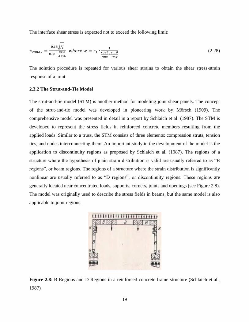
The interface shear stress is expected not to exceed the following limit:
𝑣𝑐𝑖𝑚𝑎𝑥 =0.18√𝑓𝑐
′
0.31+24𝑤
𝑎+16
𝑤ℎ𝑒𝑟𝑒 𝑤 = 휀1 ∙1
cos𝜃
𝑠𝑚𝑥+sin𝜃
𝑠𝑚𝑦
(2.28)
The solution procedure is repeated for various shear strains to obtain the shear stress-strain
response of a joint.
2.3.2 The Strut-and-Tie Model
The strut-and-tie model (STM) is another method for modeling joint shear panels. The concept
of the strut-and-tie model was developed in pioneering work by Mörsch (1909). The
comprehensive model was presented in detail in a report by Schlaich et al. (1987). The STM is
developed to represent the stress fields in reinforced concrete members resulting from the
applied loads. Similar to a truss, the STM consists of three elements: compression struts, tension
ties, and nodes interconnecting them. An important study in the development of the model is the
application to discontinuity regions as proposed by Schlaich et al. (1987). The regions of a
structure where the hypothesis of plain strain distribution is valid are usually referred to as “B
regions”, or beam regions. The regions of a structure where the strain distribution is significantly
nonlinear are usually referred to as “D regions”, or discontinuity regions. These regions are
generally located near concentrated loads, supports, corners, joints and openings (see Figure 2.8).
The model was originally used to describe the stress fields in beams, but the same model is also
applicable to joint regions.
Figure 2.8: B Regions and D Regions in a reinforced concrete frame structure (Schlaich et al.,
1987)
20
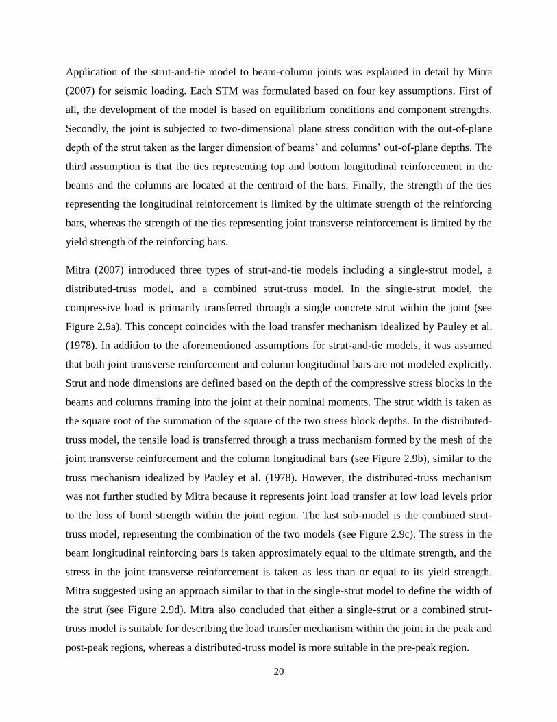
Application of the strut-and-tie model to beam-column joints was explained in detail by Mitra
(2007) for seismic loading. Each STM was formulated based on four key assumptions. First of
all, the development of the model is based on equilibrium conditions and component strengths.
Secondly, the joint is subjected to two-dimensional plane stress condition with the out-of-plane
depth of the strut taken as the larger dimension of beams’ and columns’ out-of-plane depths. The
third assumption is that the ties representing top and bottom longitudinal reinforcement in the
beams and the columns are located at the centroid of the bars. Finally, the strength of the ties
representing the longitudinal reinforcement is limited by the ultimate strength of the reinforcing
bars, whereas the strength of the ties representing joint transverse reinforcement is limited by the
yield strength of the reinforcing bars.
Mitra (2007) introduced three types of strut-and-tie models including a single-strut model, a
distributed-truss model, and a combined strut-truss model. In the single-strut model, the
compressive load is primarily transferred through a single concrete strut within the joint (see
Figure 2.9a). This concept coincides with the load transfer mechanism idealized by Pauley et al.
(1978). In addition to the aforementioned assumptions for strut-and-tie models, it was assumed
that both joint transverse reinforcement and column longitudinal bars are not modeled explicitly.
Strut and node dimensions are defined based on the depth of the compressive stress blocks in the
beams and columns framing into the joint at their nominal moments. The strut width is taken as
the square root of the summation of the square of the two stress block depths. In the distributed-
truss model, the tensile load is transferred through a truss mechanism formed by the mesh of the
joint transverse reinforcement and the column longitudinal bars (see Figure 2.9b), similar to the
truss mechanism idealized by Pauley et al. (1978). However, the distributed-truss mechanism
was not further studied by Mitra because it represents joint load transfer at low load levels prior
to the loss of bond strength within the joint region. The last sub-model is the combined strut-
truss model, representing the combination of the two models (see Figure 2.9c). The stress in the
beam longitudinal reinforcing bars is taken approximately equal to the ultimate strength, and the
stress in the joint transverse reinforcement is taken as less than or equal to its yield strength.
Mitra suggested using an approach similar to that in the single-strut model to define the width of
the strut (see Figure 2.9d). Mitra also concluded that either a single-strut or a combined strut-
truss model is suitable for describing the load transfer mechanism within the joint in the peak and
post-peak regions, whereas a distributed-truss model is more suitable in the pre-peak region.

21
Figure 2.9: The strut-and-tie model: (a) single-strut model, (b) distributed-truss model, (c)
combined strut-truss model, and (d) definition of the strut width in combined strut-truss
mechanism (Mitra, 2007)
(a) (b)
(c) (d)

22
The more complex strut-and-tie models suitable for joint application include the softened strut-
and-tie model proposed by Hwang and Lee (2002), and the compatibility strut-and-tie model
proposed by Scott et al. (2012).
2.3.3 Bond Stress-Slip Relationship
In traditional analysis of reinforced concrete frame structures subjected to seismic loading,
perfect bond between the reinforcement and the concrete is often assumed. Under severe seismic
loads, cracks form at the interface of joints and beams framing into the joints (see Figure 2.5).
Reinforcing bars at the cracks may be strained beyond their yielding point, while being
simultaneously pushed and pulled at the opposite sides of the joint, creating high bond stresses
between the longitudinal reinforcing steel and the surrounding concrete. Therefore, modeling of
the bond stress-slip relationship becomes a crucial part of effective joint modeling. Two of the
earliest studies for characterizing and modeling bond behavior were carried out by
Viwathanatepa et al. (1979) and Eligehausen et al. (1983).
Viwathanatepa et al. (1979) tested seventeen specimens of single reinforcing bars embedded in
well-confined column stubs subjected to push-pull or pull only loadings. The specimens were
made 46 inches (1168 mm) high with the width of the blocks ranging from 15 inches (381 mm)
to 25 inches (635 mm) (see Figure 2.10a). A sufficient amount of transverse reinforcement was
provided for shear and confinement. The amount of the longitudinal reinforcement was designed
to confine crack propagation, limit crack size, and provide strength to resist the applied flexural
bending moment. Adequate anchorage length was provided to ensure that the maximum steel
stress could be developed. The supports were also designed to minimize the stress concentration
developed in the test specimen. The load was applied to the specimens by three hydraulic jacks
(see Figure 2.10b). The authors were mainly interested in three aspects of the results: the load-
displacement response measured at the protruding end of the bar, the stress and strain
distributions along the longitudinal reinforcing bars, and the bond stress distribution along the
rebar.

23
Figure 2.10: Test setup in the bond experiment conducted by Viwathanatepa et al. (1979): (a)
the elevation view of the specimen and (b) the testing apparatus
For the push-pull loading under a monotonic loading history, Viwathanatepa et al. concluded that:
(1) the application of a pushing load in addition to a pulling load has little effect from a strength
point of view; (2) the application of a pushing load reduces the pull-out ductility; (3) the smaller
the bar size, the higher the average bond strength that could be developed; and (4) the bond stress
of grooved bars (i.e. bars with reduced effective perimeter and cross-sectional area) may differ
by 15% from that of ungrooved bars. Ultimately, Viwathanatepa et al. formulated a bond stress-
slip relationship as a step towards determining the load-displacement relationship at the exposed
ends of a reinforcing bar embedded in a concrete block subjected to either monotonic or reversed
cyclic loading. The actual behavior was idealized as a round bar surrounding by two layers of
soft concrete which consisted of an unconfined region near the pull end, a pushed end region and
a confined region in the middle. A four-stage monotonic skeleton bond stress-slip curve was
constructed based on the response of the three regions (see Figure 2.11a). The curve was further
modified using reduction factors and hysteric rules in order to adapt reversed cyclic loading. The
soft concrete layers were divided into finite number of elements to be analyzed individually (see
Figure 2.11b). The forces and local displacements of the corresponding spring elements are
calculated as follows:
(a) (b)

24
𝐹 = 𝜏𝐶𝑙𝑒 (2.29)
𝛿 = 𝛾𝑡 (2.30)
where 𝐹 is the force in the spring element, 𝛿 is the local displacement of the spring element, 𝜏 is
the shear stress of the soft layer element, 𝛾 is the shear deformation of the soft layer element, 𝐶 is
the circumference of the rebar, 𝑙𝑒 is the length of the soft layer element and 𝑡 is the thickness of
the soft layer. The sum of the results from the individual springs denotes the load-displacement
relationship at the exposed ends of a reinforcing bar embedded in concrete (see Figure 2.11c).
Figure 2.11: Formulation of bond model proposed by Viwathanatepa et al. (1979): (a)
monotonic skeleton bond stress-slip Curve, (b) finite soft layer elements, and (c) load-
displacement relationship of a #8 (25M) bar
(a) (b)
(c)

25
Eligenhausen et al. (1983) tested 125 pull-out specimens loaded at one end of the reinforcing bar
embedded in concrete blocks. The objective was to study the local bond-stress relationship of
deformed bars embedded in confined concrete subjected to monotonic and cyclic loading
conditions, and create an analytical model for the bond behavior. The test program was similar to
that of Viwathanatepa et al. (1979). Eligenhausen et al. (1983) presented the influence of seven
parameters on the bond stress-slip relationship for monotonic loading, as follows:
(1) Tension or compression loading: The bond stress-slip relationships are approximately
equal for bars a in tension or compression prior to yielding. After yielding, the bond
resistance of bar in tension reduces significantly, whereas the bond resistance of a bar in
compression increases.
(2) Confining reinforcement: The confining reinforcement increases the bond stress required
to develop splitting cracks. However, there is an upper limit for effective confining
reinforcement beyond which the bond behavior cannot be improved further.
(3) Bar diameter: The bond resistance for bars with different diameters is slightly different in
terms of the initial stiffness and the peak resistance.
(4) Concrete strength: The initial stiffness and the overall bond resistance increase with
increasing concrete strength.
(5) Bar spacing: The bond behavior improves with increasing bar spacing, but the
improvement is relatively small.
(6) Transverse pressure: Transverse pressure helps develop greater bond resistance while
other conditions remain unchanged.
(7) Rate of pull-out: The bond resistance increases with the increasing rate of bar pull-out.
For cyclic loading, considerations were also given in this study to the behavior in the unloading
branch and in the reloading branch. The analysis of the influence of each parameter was also
provided in this study.
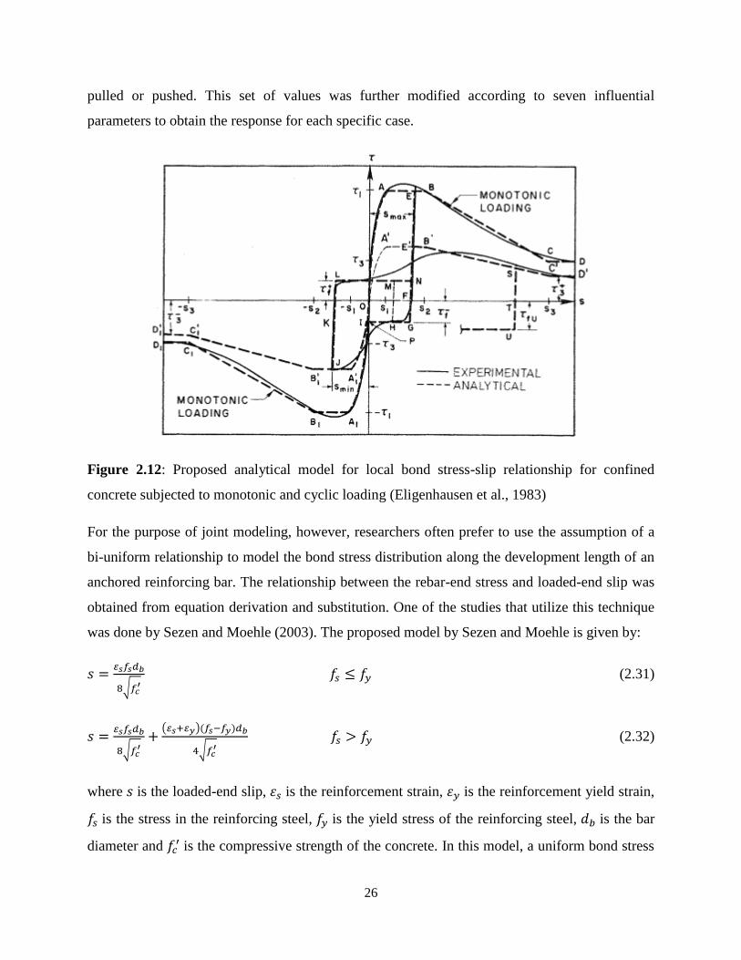
Eligenhausen et al. (1983) further characterized the mechanism of bond resistance for both
monotonic and cyclic loading, and proposed a general analytical model for the local bond stress-
slip relationship for confined concrete (see Figure 2.12). In this model, a set of values was
provided with the same bond stress-slip relationship assumed regardless of whether the bar was
26
pulled or pushed. This set of values was further modified according to seven influential
parameters to obtain the response for each specific case.
Figure 2.12: Proposed analytical model for local bond stress-slip relationship for confined
concrete subjected to monotonic and cyclic loading (Eligenhausen et al., 1983)
For the purpose of joint modeling, however, researchers often prefer to use the assumption of a
bi-uniform relationship to model the bond stress distribution along the development length of an
anchored reinforcing bar. The relationship between the rebar-end stress and loaded-end slip was
obtained from equation derivation and substitution. One of the studies that utilize this technique
was done by Sezen and Moehle (2003). The proposed model by Sezen and Moehle is given by:
𝑠 =𝜀𝑠𝑓𝑠𝑑𝑏
8√𝑓𝑐′ 𝑓𝑠 ≤ 𝑓𝑦 (2.31)
𝑠 =𝜀𝑠𝑓𝑠𝑑𝑏
8√𝑓𝑐′+(𝜀𝑠+𝜀𝑦)(𝑓𝑠−𝑓𝑦)𝑑𝑏
4√𝑓𝑐′
𝑓𝑠 > 𝑓𝑦 (2.32)
where 𝑠 is the loaded-end slip, 휀𝑠 is the reinforcement strain, 휀𝑦 is the reinforcement yield strain,
𝑓𝑠 is the stress in the reinforcing steel, 𝑓𝑦 is the yield stress of the reinforcing steel, 𝑑𝑏 is the bar
diameter and 𝑓𝑐′ is the compressive strength of the concrete. In this model, a uniform bond stress

27
of 1.0√𝑓𝑐 was assumed in the elastic range, whereas a uniform bond stress of 0.5√𝑓𝑐 was used in
post-yielding range. Another bar stress versus loaded-end slip model, which was based on curve
fitting and experimental observations, was proposed by Zhao and Sritharan (2007). The
monotonic envelope curve was composed of a straight line for the elastic region and a curvilinear
portion for the post-yielding region (see Figure 2.13), as follows:
𝑓𝑠 = 𝐾𝑠 𝑓𝑠 ≤ 𝑓𝑦 (2.33)
𝑓𝑠 = �� ∙ (𝑓𝑢 − 𝑓𝑦) + 𝑓𝑦 𝑓𝑠 > 𝑓𝑦 (2.34)
where 𝑓𝑠 is the stress in the reinforcing steel, 𝑠 is the loaded-end slip, 𝑓𝑦 is the yield stress of the
reinforcing steel, 𝑓𝑢 is the ultimate stress of the reinforcing steel, 𝐾 is the slope of the straight
line and �� is the normalized bar stress.
Figure 2.13: Monotonic envelope curve of bar stress versus loaded-end slip relationship (Zhao
and Sritharan, 2007)

28
2.4 Review of Existing Beam-Column Joint Models
Many researchers have proposed various beam-column joint models over the past two decades.
These models can be categorized into three types: (1) rotational hinge models such as by Alath
and Kunnath (1995), Altoontash (2004) and Shin and LaFave (2004); (2) component models
such as by Youssef and Ghobarah (2001), Lowes and Altoontash (2003) and Mitra and Lowes
(2007); and (3) finite element models. Rotational hinge models are non-objective and require
calibration for each specific type of joint. Finite element models are complex and require
significant computational resources; therefore, they are not suitable for holistic frame analysis.
Component models provide a good balance between simplicity and accuracy. They are generally
objective and suitable for analyzing large frames. They use mechanics-based formulations and
generally do not require calibration for each particular joint type.
2.4.1 Rotational Hinge Models
2.4.1.1 Alath and Kunnath (1995)
Alath and Kunnath modeled the joint with four rigid links representing the joint panel geometry,
and a zero-length rotational spring with a degrading hysteresis rule representing the joint shear
deformations (see Figure 2.14). The joint shear stress-strain relationship was determined
empirically, while the cyclic response was captured with a hysteretic model that was calibrated
by experiments. The model was validated through a study comparing the analytical and
experimental response of an interior beam-column joint subassembly. One disadvantage of this
model is that it only considers the joint shear behavior, neglecting the bond slip behavior.
Figure 2.14: Joint model proposed by Alath and Kunnath (Alath and Kunnath, 1995; figure
adopted from Celik and Ellingwood, 2008)
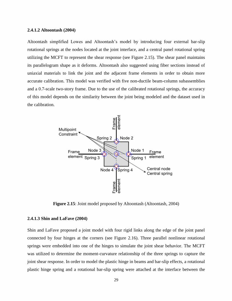
29
2.4.1.2 Altoontash (2004)
Altoontash simplified Lowes and Altoontash’s model by introducing four external bar-slip
rotational springs at the nodes located at the joint interface, and a central panel rotational spring
utilizing the MCFT to represent the shear response (see Figure 2.15). The shear panel maintains
its parallelogram shape as it deforms. Altoontash also suggested using fiber sections instead of
uniaxial materials to link the joint and the adjacent frame elements in order to obtain more
accurate calibration. This model was verified with five non-ductile beam-column subassemblies
and a 0.7-scale two-story frame. Due to the use of the calibrated rotational springs, the accuracy
of this model depends on the similarity between the joint being modeled and the dataset used in
the calibration.
Figure 2.15: Joint model proposed by Altoontash (Altoontash, 2004)
2.4.1.3 Shin and LaFave (2004)
Shin and LaFave proposed a joint model with four rigid links along the edge of the joint panel
connected by four hinges at the corners (see Figure 2.16). Three parallel nonlinear rotational
springs were embedded into one of the hinges to simulate the joint shear behavior. The MCFT
was utilized to determine the moment-curvature relationship of the three springs to capture the
joint shear response. In order to model the plastic hinge in beams and bar-slip effects, a rotational
plastic hinge spring and a rotational bar-slip spring were attached at the interface between the
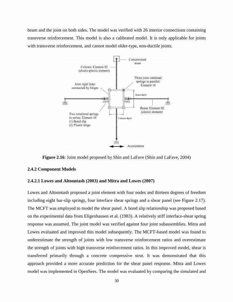
30
beam and the joint on both sides. The model was verified with 26 interior connections containing
transverse reinforcement. This model is also a calibrated model. It is only applicable for joints
with transverse reinforcement, and cannot model older-type, non-ductile joints.
Figure 2.16: Joint model proposed by Shin and LaFave (Shin and LaFave, 2004)
2.4.2 Component Models
2.4.2.1 Lowes and Altoontash (2003) and Mitra and Lowes (2007)
Lowes and Altoontash proposed a joint element with four nodes and thirteen degrees of freedom
including eight bar-slip springs, four interface shear springs and a shear panel (see Figure 2.17).
The MCFT was employed to model the shear panel. A bond slip relationship was proposed based
on the experimental data from Eligenhausen et al. (1983). A relatively stiff interface-shear spring
response was assumed. The joint model was verified against four joint subassemblies. Mitra and
Lowes evaluated and improved this model subsequently. The MCFT-based model was found to
underestimate the strength of joints with low transverse reinforcement ratios and overestimate
the strength of joints with high transverse reinforcement ratios. In this improved model, shear is
transferred primarily through a concrete compressive strut. It was demonstrated that this
approach provided a more accurate prediction for the shear panel response. Mitra and Lowes
model was implemented in OpenSees. The model was evaluated by comparing the simulated and

31
observed responses of 57 previous experimental specimens of interior joints. Although this
model is capable of predicting the response of joints under monotonic and cyclic loading, it has
three drawbacks: complicated definition of the model parameters, intra-element solution
procedure, and potential numerical convergence problems under cyclic loading.
Figure 2.17: Joint model proposed by Lowes and Altoontash (Lowes and Altoontash, 2003)
2.4.2.2 Ghobarah and Youssef (2001)
Ghobarah and Youssef proposed a joint element with two diagonal springs linking the opposite
corners of the joint element (see Figure 2.18). The MCFT was employed to simulate the shear
deformations in the joint panel zone. Three sets of concrete and steel springs were used at each
side of the joint perimeter to account for the bond-slip effects. The joint model, along with a
proposed structural wall model, was incorporated in a structural analysis program and verified
with a three-story non-ductile frame. This model requires a large amount of springs with separate
constitutive models, which may limit its applicability.

32
Figure 2.18: Joint model proposed by Ghobarah and Youssef (Ghobarah and Youssef, 2001)
2.4.2.3 Fleury et al. (2000)
Fleury et al. proposed a multi-component model for the simulation of multiple components
consisting of a single joint element and the surrounding components (see Figure 2.19). The joint
core behavior was described by a concrete element and a transverse reinforcement element. A
series of elements was used to describe the longitudinal reinforcing steel in the beam members
and its bond throughout the joint. The longitudinal reinforcing steel was represented by two-node
bar elements. The connections of the beams to the joint were also represented by two elements.
All these elements were connected by an imposed relationship between degrees of freedom. This
model was applied to an interior beam-column connection containing transverse reinforcement.
The consideration of bond slip helps the model obtain satisfactory estimation of the dissipated
energy. This joint model is also overly complex for the implementation in this study because it
involves the simulation of various types of elements and the relationships among all these
elements.

33
Figure 2.19: Joint model proposed by Fleury et al. (Fleury et al., 2000)
2.4.2.4 Elmorsi et al. (2000)
Elmorsi et al. proposed a 12-node multi-component model to represent the beam-column joint
response (see Figure 2.20a). The joint element employs a fixed, smeared-crack concrete
constitutive model for the normal stress function and the shear stress function. This joint element
is connected to beams and columns with ten transitional nodes representing the plastic hinge
regions in the beams and the columns. The beams and columns were modeled with elastic beam
line elements, and the flexural reinforcement was modeled with inelastic truss elements. Contact
elements connecting the joint nodes and the transition nodes were used to model the bond slip
effects (see Figure 2.20b). The bond slip material model was a modified version based on the
Eligenhausen et al. (1983) model. This analytical model was verified against the experimental
data from Viwathanatepa et al. (1979). The joint element demonstrated good correlation between
the predictions and experimental data of two interior beam-column subassemblies in terms of
strength and bond slip deformations. However, this model is relatively complex and may require
significant analysis time for large frames.
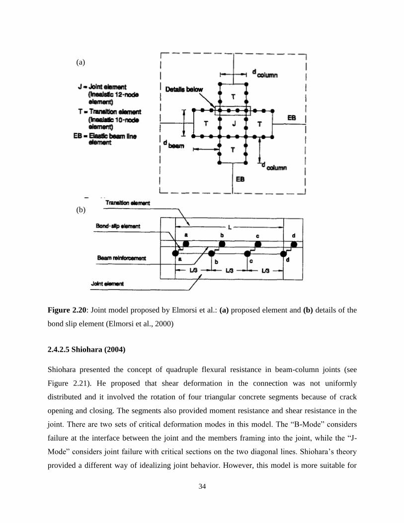
34
Figure 2.20: Joint model proposed by Elmorsi et al.: (a) proposed element and (b) details of the
bond slip element (Elmorsi et al., 2000)
2.4.2.5 Shiohara (2004)
Shiohara presented the concept of quadruple flexural resistance in beam-column joints (see
Figure 2.21). He proposed that shear deformation in the connection was not uniformly
distributed and it involved the rotation of four triangular concrete segments because of crack
opening and closing. The segments also provided moment resistance and shear resistance in the
joint. There are two sets of critical deformation modes in this model. The “B-Mode” considers
failure at the interface between the joint and the members framing into the joint, while the “J-
Mode” considers joint failure with critical sections on the two diagonal lines. Shiohara’s theory
provided a different way of idealizing joint behavior. However, this model is more suitable for
(a)
(b)

35
hand calculations rather than software implementation. In addition, verification studies are not
available for this model.
Figure 2.21: Joint model proposed by Shiohara (Shiohara, 2004)

36
CHAPTER 3
IMPLEMENTED JOINT ELEMENT MODEL
3.1 Chapter Layout
After review of the current state-of-the-art for the modeling of interior beam-column joints of
reinforced concrete frame structures, the model proposed by Mitra and Lowes (2007) was
selected to be implemented in a previously-developed global frame analysis procedure. This
chapter will introduce the theoretical principles and mathematical formulation of the joint
element model implemented.
Mitra and Lowes modified and improved the model proposed by Lowes and Altoontash (2003).
This component model is capable of capturing bond slip response and joint shear actions in the
joint region. Although the model is applicable to frames subjected to reversed cyclic loading, this
chapter, and this study, focuses on the monotonic response as a foundation to understand the
performance of the implementation of this model. The chapter starts with an introduction to the
joint element formulation, and continues with the modeling of three types of components
including bar slip springs, a shear panel component and the interface shear springs. Finally, a
summary of the computation schemes to simulate the joint response under monotonic loading is
provided at the end of the chapter.
3.2 Joint Element Formulation
The implemented beam-column joint model adopts the model proposed by Mitra and Lowes
(2007), which was modified and improved based on the model proposed by Lowes and
Altoontash (2003). This is a four node, thirteen degree-of-freedom component model that
consists of eight zero-length bar slip springs which simulate the strength and stiffness loss of
bond between concrete and reinforcing bars, four interface shear springs which simulate the
shear transfer from beams and columns to the joint, and a panel element which simulate shear
deformation in the joint region (see Figure 3.1). This model represents the inelastic actions

37
taking place in joints including mechanisms of joint core shear resistance and bond slip response.
Although the joint element represents actions in an interior joint, the formulation is also
applicable to exterior joints and knee joints with some modifications, which are not discussed in
detail in the original study. Mitra and Lowes evaluated this model by comparing simulated and
observed responses over 57 previous experimental investigations of interior joints consisting of
52 specimens with transverse reinforcement and 5 specimens without transverse reinforcement.
They concluded that the model provided good results in terms of the failure mechanism, stiffness
of the overall structure, maximum strength, drift at maximum strength and the pinching ratio.
This model was found suitable for the implementation into the global frame analysis procedure
of VecTor5 given that the required input for the local joint element is already calculated by the
global procedure.
Figure 3.1: Implemented interior beam-column joint model (Mitra and Lowes, 2007)
The solution of this model requires finding component deformations and the corresponding
material state of the joint element. The joint element is formulated based on compatibility,
equilibrium and constitutive relationships. Compatibility of the element requires the four external
nodal displacements to be compatible with the thirteen component deformations. Equilibrium of
the element needs to be satisfied at four external and four internal nodes. Constitutive
relationships, which consist of a bond slip response and a joint shear response, relate the
Shear Panel Beam Element Beam Element
Co
lum
E
lem
ent
External
Node
Internal
Node
Zero-length
Bar slip Spring
Zero-length
Interface Shear
Spring
Co
lum
E
lem
ent
1 2 4
5
7 8
9
10
11
12 13
6
3
Degree of Freedom

38
component deformations to the component forces. A representation of the displacement,
deformation and force variables is illustrated in Figure 3.2.
Figure 3.2: Definition of displacements, deformations and forces in the model: (a) external
displacements and component deformations and (b) external forces and component forces
Deformation of the joint element components is defined by the external nodal displacements. A
positive deformation of the bar slip component is associated with a tensile force applied to the
bars. A positive shear deformation of the panel component is associated with the positive shear
forces at the internal nodes in the joint core. A positive deformation of the interface shear
component is associated with the positive external shear displacement. The twelve external
displacements and rotations, 𝑢𝑖, are converted to thirteen component deformations, ∆𝑖, using the
following equations proposed by Mitra and Lowes:
∆1= −𝑢2 +��
2𝑢3 +
��
2(𝑣4−𝑣2
𝑤) +
𝑣4+𝑣2
2 (3.1a)
∆2= −𝑢2 −��
2𝑢3 +
��
2(𝑣2−𝑣4
𝑤) +
𝑣4+𝑣2
2 (3.1b)
∆3= 𝑢1 − 𝑣1 (3.1c)
∆4= 𝑢4 +ℎ
2𝑢6 −
ℎ
2(𝑣1−𝑣3
ℎ) −
𝑣1+𝑣3
2 (3.1d)
u1 u
2
u3
u4
u5
u6
u7
u8
u9
u10
u
11
u12
Δ1 Δ
2 Δ
3
Δ4
Δ5
Δ6
Δ7 Δ
8
Δ9
Δ10
Δ11
Δ12
Δ13
v1
v2
v3
v4
F1
F2
F3
F4
F5
F6
F7 F
9
F10
F
11
f1 f
2 f
3
f4
f5
f6
f7 f
8
f9
f10
f11
f12
f13
φ1
φ 2
φ 3
φ 4
F8
F12
(a) (b)

39
∆5= 𝑢4 −ℎ
2𝑢6 −
ℎ
2(𝑣3−𝑣1
ℎ) −
𝑣1+𝑣3
2 (3.1e)
∆6= 𝑢5 − 𝑣2 (3.1f)
∆7= 𝑢8 −��
2𝑢9 +
��
2(𝑣2−𝑣4
𝑤) −
𝑣2+𝑣4
2 (3.1g)
∆8= 𝑢8 +��
2𝑢9 −
��
2(𝑣2−𝑣4
𝑤) −
𝑣2+𝑣4
2 (3.1h)
∆9= 𝑢7 − 𝑣3 (3.1i)
∆10= −𝑢10 −ℎ
2𝑢12 +
ℎ
2(𝑣1−𝑣3
ℎ) +
𝑣1+𝑣3
2 (3.1j)
∆11= −𝑢10 +ℎ
2𝑢12 −
ℎ
2(𝑣1−𝑣3
ℎ) +
𝑣1+𝑣3
2 (3.1k)
∆12= 𝑢11 − 𝑣4 (3.1l)
∆13= −𝑣1
ℎ+𝑣2
𝑤+𝑣3
ℎ−𝑣4
𝑤 (3.1m)
where v is the internal nodal displacement, ℎ is the height of the joint, 𝑤 is the width of the joint,
ℎ is the distance between the bar slip springs on the beam side, and �� is the distance between
the bar slip springs on the column side. In the Lowes and Altoontash model, the width and the
height are used instead of the distances between the bar slip springs. This modification is made
in the Mitra and Lowes model to improve the simulation of the bar slip spring force demands.
The thirteen equations can also be written in a matrix representation as follows:
[∆13𝑋1] = [𝐴13𝑋16] [𝑢12𝑋1𝑣4𝑋1
] (3.2)
where 𝐴 is the transformation matrix that converts the nodal displacements to component
deformations. Figure 3.3 illustrates the expanded matrix formulation of this equation.
Similarly, the external and internal nodal resultants are computed from the component forces by
imposing the equilibrium conditions on the four external and four internal nodes. The material
state of the shear panel component, which is assumed to deform only in shear, implies that the
internal nodal resultants equal to zero. The equilibrium equations proposed by Mitra and Lowes
are listed as follows:

40
Figure 3.3: Compatibility equations of the implemented joint model (Mitra and Lowes, 2007)
𝐹1 = 𝑓3 (3.3a)
𝐹2 = −𝑓1−𝑓2 (3.3b)
𝐹3 =��
2(𝑓2 − 𝑓1) (3.3c)
𝐹4 = 𝑓4+𝑓5 (3.3d)
𝐹5 = 𝑓6 (3.3e)
𝐹6 =ℎ
2(𝑓4 − 𝑓5) (3.3f)
𝐹7 = 𝑓9 (3.3g)
𝐹8 = 𝑓7+𝑓8 (3.3h)
𝐹9 =��
2(𝑓8 − 𝑓7) (3.3i)
𝐹10 = −𝑓10−𝑓11 (3.3j)

41
𝐹11 = 𝑓12 (3.3k)
𝐹12 =ℎ
2(𝑓11 − 𝑓10) (3.3l)
𝜑1 = −𝑓3 −1
2(1 +
ℎ
ℎ)(𝑓4 − 𝑓10) −
1
2(1 −
ℎ
ℎ)(𝑓5 − 𝑓11) −
𝑓13
ℎ (3.3m)
𝜑2 = −𝑓6 −1
2(1 +
��
𝑤)(𝑓8 − 𝑓2) −
1
2(1 −
��
𝑤)(𝑓7 − 𝑓1) +
𝑓13
𝑤 (3.3n)
𝜑3 = −𝑓9 −1
2(1 +
ℎ
ℎ)(𝑓5 − 𝑓11) −
1
2(1 −
ℎ
ℎ)(𝑓4 − 𝑓10) +
𝑓13
ℎ (3.3o)
𝜑4 = −𝑓12 −1
2(1 +
��
𝑤)(𝑓7 − 𝑓1) −
1
2(1 −
��
𝑤)(𝑓8 − 𝑓2) −
𝑓13
𝑤 (3.3p)
where 𝐹𝑖 is the external nodal resultant, 𝑓𝑖 is the component force and 𝜑𝑖 is the interior nodal
resultant which equals to zero at the equilibrium state. The sixteen equations can also be written
in a matrix representation as follows:
[𝐹12𝑋1𝜑4𝑋1
] = [𝐴𝑇16𝑋13][𝑓13𝑋1] (3.4)
where 𝐴𝑇 is the transposed transformation matrix that converts the component forces to nodal
resultants. A vector of external nodal resultants is obtained in this process. The derivative of the
resultants with respect to the external nodal displacements, also known as the element tangent
matrix, is calculated as follows:
[𝐾𝑒𝑙𝑒𝑚 16𝑋16] = [𝐴𝑇16𝑋13][𝑘13𝑋13][𝐴13𝑋16] 𝑤ℎ𝑒𝑟𝑒 𝑘𝑖 =
𝑑𝑓𝑖
𝑑∆𝑖, 𝑖 = 1,2, … , 13 (3.5)
In this equation, 𝐾𝑒𝑙𝑒𝑚 is the element tangent matrix, 𝐴 is the transformation matrix and 𝑘 is a
diagonal matrix of thirteen component tangents.
3.3 Modeling Bond Slip Response
Modeling of bond slip effect is crucial for the simulation of inelastic beam-column joint response.
During an earthquake event, tensile stress at one end of a reinforcing bar may penetrate into the
joint region. This causes significant elongation of the reinforcement. Furthermore, the bond

42
between the reinforcing steel and concrete may deteriorate and cause addition deformation. The
combination of these two effects is referred to as “strain penetration”. The bar slip springs in the
joint element are utilized to represent this action.
The bond slip model developed by Mitra and Lowes was based on the experimental data of
Elighausen et al. (1983) and four assumptions about the bond stress distribution (see Figure 3.4)
including: (1) bond slip is defined as the relative movement of the reinforcing steel with respect
to the interface of the joint; (2) the model only considers the contribution from the elongation of
the reinforcement; (3) the reinforcing bar is assumed to have zero slip at zero bar stress; and (4)
the bond stress is assumed to be uniform prior to yielding of the reinforcing steel and piecewise
uniform after yielding.
The bar stress and slip model was derived based on the equilibrium condition of the force
transferred from the concrete to the reinforcing steel and the force carried by the reinforcing steel,
as follows:
𝐹𝑠 = 𝑓𝑠 ∙𝜋𝑑𝑏2
4= 𝜇𝜋𝑑𝑏𝑙𝑑 (3.6)
where 𝐹𝑠 is the force carried by the reinforcing steel, 𝑓𝑠 is the stress in the reinforcing steel, 𝑑𝑏is
the diameter of the bar, 𝜇 is the bond stress, and 𝑙𝑑 is the development length of the bar to
transfer the force through bond stress. The reinforcing steel material model is assumed to be
plastic with elastic hardening. By writing the equilibrium equation in terms of strain in the
reinforcing steel and integrating the strain from the anchorage point to the joint interface, the
relationship between the bar stress and slip is obtained. The model proposed by Mitra and Lowes
is summarized below.
∆𝑠𝑙𝑖𝑝= 2𝜏𝐸
𝐸
𝑙𝑓𝑠2
𝑑𝑏 𝑓𝑜𝑟 𝑓𝑠 < 𝑓𝑦 (3.7a)
∆𝑠𝑙𝑖𝑝= 2𝜏𝐸
𝐸
𝑙𝑒2
𝑑𝑏+𝑓𝑦𝑙𝑦
𝐸+ 2
𝜏𝑌
𝐸𝑠ℎ
𝑙𝑦2
𝑑𝑏 𝑓𝑜𝑟 𝑓𝑠 ≥ 𝑓𝑦 (3.7b)

43
𝑤ℎ𝑒𝑟𝑒 𝑙𝑓𝑠 =𝑓𝑠
𝜏𝐸𝑇
𝐴𝑏
𝜋𝑑𝑏 (3.7c)
𝑙𝑒 =𝑓𝑦
𝜏𝐸𝑇
𝐴𝑏
𝜋𝑑𝑏 (3.7d)
𝑙𝑦 =𝑓𝑠−𝑓𝑦
𝜏𝑌𝑇
𝐴𝑏
𝜋𝑑𝑏 (3.7e)
Figure 3.4: Bond stress and bar stress distribution along a reinforcing bar anchored in a joint
In this set of equations, ∆𝑠𝑙𝑖𝑝 is the slip of the reinforcing steel at the joint interface, 𝑓𝑠 is the
stress in the reinforcing steel at the interface of the joint, 𝑓𝑦 is the yield stress of steel, 𝐸 is the
modulus of elasticity of steel, 𝐸𝑠ℎ is the hardening modulus of steel, 𝑑𝑏 is the nominal bar
diameter, 𝐴𝑏 is the nominal bar area, 𝜏𝐸 is the bond stress of elastic steel, and 𝜏𝑌 is the bond
stress of post-yielding steel. Average bond stress values for various rebar conditions are listed in
Table 3.1. Figure 3.5 shows the proposed bar stress versus slip model, the model from Sezen and
Moehle (2003), and the experimental data provided by Viwathanatepa et al. (1979).
fsAb
le l
y
fs
fy
τET
τ
YT
fc
lfs_comp
τEC
bond
stress
bar
stress
Column Rebar
Beam Rebar

44
Table 3.1: Average bond stress for various rebar conditions
Rebar Condition Average Bond Stress in MPa (𝒇𝒄 in MPa)
Tension, Elastic Rebar
Tension, Post-Yielding Rebar
Compression, Elastic Rebar
Compression, Post-Yielding Rebar
𝜏𝐸𝑇 = 1.8√𝑓𝑐
𝜏𝑌𝑇 = 0.4√𝑓𝑐 𝑡𝑜 0.05√𝑓𝑐
𝜏𝐸𝐶 = 2.2√𝑓𝑐
𝜏𝑌𝐶 = 3.6√𝑓𝑐
Figure 3.5: Bar stress versus slip relationship from various studies and experiments
The bar stress versus slip model for monotonic loading presented in Mitra and Lowes is similar
to that presented in Lowes and Altoontash. The only difference is the initiation of the strength
loss in the response. The Lowes and Altoontash model used a slip limit of 3.0 mm, which was
found to be too conservative. The Mitra and Lowes delayed the initiation of the strength loss
until the reinforcing steel reaches its ultimate strength. On the other hand, this model also
improved the reversed cyclic response of the bar slip springs. Mitra and Lowes defined the
unloading and reloading path and a damage model to represent the influence of load history on
the response. These parameters are crucial for successful modeling of the reversed cyclic
response.
0
100
200
300
400
500
600
700
0 2 4 6 8 10
Bar
Str
ess
(MP
a)
Slip (mm)
Mitra and Lowes (2007)
Lowes and Altoontash (2003)
Sezen and Moehle (2003)
Viwathanatepa et al. (1979)

45
The bar stress is finally related to the force in bar slip springs to complete the calculation.
Determination of the magnitude and location of the bar slip springs requires sectional analysis of
the beam and column members framing into the joint at nominal flexural strength. The
computation of nominal flexural strength follows the criteria of ACI Committee 318 (2008). The
ACI code was employed over the CSA code because the study was conducted in the United
States. It is expected that the CSA criteria will produce similar results because the CSA criteria
are similar to the ACI criteria. According to the criteria, a linear strain distribution is assumed
across the section of a member with the top concrete strain set at -0.003. The compressive stress
block approach is employed to determine the compressive force carried by the concrete, and
tension stiffening is neglected for simplicity. Using the ACI criteria, the concrete and steel
compression resultants are defined as follows:
𝐶𝑐 = 0.85𝑓𝑐′𝛽𝑐𝑤 (3.8)
𝐶𝑠′ = 𝑓𝑠
′𝐴𝑠′ = 0.003
𝑐−𝑑′
𝑐𝐸𝑠𝐴𝑠
′ (3.9)
where 𝐶𝑐 is the total compressive force carried by the concrete, 𝐶𝑠′ is the total compressive force
carried by the reinforcing steel, 𝑓𝑐′ is the concrete compressive strength, 𝑐 is the depth of neutral
axis, 𝑑′ is the depth of the reinforcing steel carrying compression, 𝐸𝑠 is the modulus of elasticity
of steel, and 𝐴𝑠′ is the area of the reinforcing steel carrying compression. The compressive and
tensile resultants, or bar slip spring forces, are defined as a function of the bar stress, given by:
𝐶𝑟𝑒𝑠𝑢𝑙𝑡𝑎𝑛𝑡 = 𝐶𝑠′ + 𝐶𝑐 = 𝑓𝑠
′𝐴𝑠′ {1 +
0.85𝑓𝑐′𝑑𝑤
𝐸𝑠𝐴𝑠′
2(1−𝑗)
0.003𝛽[1−𝑑′
𝑑
𝛽
2(1−𝑗)]} (3.10)
𝑇𝑟𝑒𝑠𝑢𝑙𝑡𝑎𝑛𝑡 = 𝑓𝑠𝐴𝑠 (3.11)
where 𝑗 is a constant taken as 0.85 for beams and 0.75 for columns, 𝛽 is the depth coefficient of
the stress block, 𝑓𝑠′ is the bar stress of the reinforcing steel carrying compression, 𝑓𝑠 is the bar
stress of the reinforcing steel carrying tension, and 𝐴𝑠 is the area of the reinforcing steel carrying
tension. The location of bar slip springs is identical to the location of the compression and
tension resultants. Figure 3.6 illustrates the strain distribution, stress distribution and forces
acting on a frame member at the nominal flexural strength.

46
Figure 3.6: Sectional analysis of a frame member at the nominal flexural strength: (a) member
cross-section, (b) strain distribution, (c) stress distribution, and (d) forces on the member
3.4 Modeling Joint Shear Response
Determination of the shear panel response requires the relationship between the shear-equivalent
moment (i.e. moment due to shear force couple acting on the joint panel) and panel shear
deformation. In the Lowes and Altoontash model, the Modified Compression Field Theory was
employed to calibrate the joint shear response model as a function of the concrete material
properties, the reinforcing steel material properties, and the reinforcing ratio in the vertical and
horizontal directions. The subsequent study by Mitra and Lowes suggested that the MCFT-based
joint shear models underestimates the strength of joints with low transverse reinforcement ratios
and overestimate the strength of joints with high transverse reinforcement ratios. In the Mitra and
Lowes model, joint shear is transferred via a concrete compression strut as shown in Figure 3.7.
The concrete strut is confined by the longitudinal reinforcing steel in the joint due to the beam
and column members framing into the joint, and the transverse reinforcement in the joint region.
The stress-strain model proposed by Mander et al. (1988) for the uniaxially confined concrete is
employed to determine the stress in the strut. Because of the confinement, the stress obtained
using the model is generally greater than that obtained from the classic parabolic stress-strain
model for joints with transverse reinforcement. Mitra and Lowes’ study does not provide the
details of the application of this stress-strain model.
w
d
εct = -0.003
εs’
εs
c
fc
fs
’
βc
fs
Cc
Cs’
Ts
Mmember
Pmember
(a) (b) (c) (d)
d’
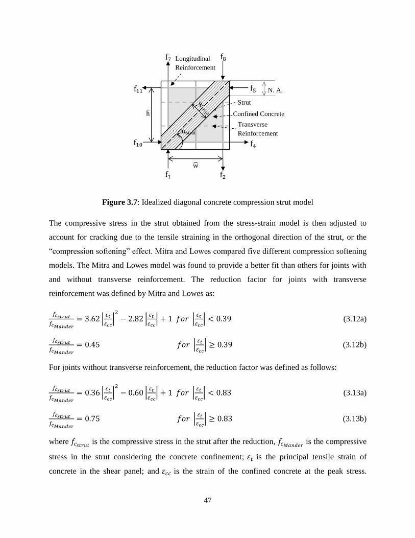
47
Figure 3.7: Idealized diagonal concrete compression strut model
The compressive stress in the strut obtained from the stress-strain model is then adjusted to
account for cracking due to the tensile straining in the orthogonal direction of the strut, or the
“compression softening” effect. Mitra and Lowes compared five different compression softening
models. The Mitra and Lowes model was found to provide a better fit than others for joints with
and without transverse reinforcement. The reduction factor for joints with transverse
reinforcement was defined by Mitra and Lowes as:
𝑓𝑐𝑠𝑡𝑟𝑢𝑡
𝑓𝑐𝑀𝑎𝑛𝑑𝑒𝑟= 3.62 |
𝜀𝑡
𝜀𝑐𝑐|2
− 2.82 |𝜀𝑡
𝜀𝑐𝑐| + 1 𝑓𝑜𝑟 |
𝜀𝑡
𝜀𝑐𝑐| < 0.39 (3.12a)
𝑓𝑐𝑠𝑡𝑟𝑢𝑡
𝑓𝑐𝑀𝑎𝑛𝑑𝑒𝑟= 0.45 𝑓𝑜𝑟 |
𝜀𝑡
𝜀𝑐𝑐| ≥ 0.39 (3.12b)
For joints without transverse reinforcement, the reduction factor was defined as follows:
𝑓𝑐𝑠𝑡𝑟𝑢𝑡
𝑓𝑐𝑀𝑎𝑛𝑑𝑒𝑟= 0.36 |
𝜀𝑡
𝜀𝑐𝑐|2
− 0.60 |𝜀𝑡
𝜀𝑐𝑐| + 1 𝑓𝑜𝑟 |
𝜀𝑡
𝜀𝑐𝑐| < 0.83 (3.13a)
𝑓𝑐𝑠𝑡𝑟𝑢𝑡
𝑓𝑐𝑀𝑎𝑛𝑑𝑒𝑟= 0.75 𝑓𝑜𝑟 |
𝜀𝑡
𝜀𝑐𝑐| ≥ 0.83 (3.13b)
where 𝑓𝑐𝑠𝑡𝑟𝑢𝑡 is the compressive stress in the strut after the reduction, 𝑓𝑐𝑀𝑎𝑛𝑑𝑒𝑟 is the compressive
stress in the strut considering the concrete confinement; 휀𝑡 is the principal tensile strain of
concrete in the shear panel; and 휀𝑐𝑐 is the strain of the confined concrete at the peak stress.
N. A.
h
w f1 f2
f4
f5
f7 f8
f10
f11
Longitudinal
Reinforcement
Transverse
Reinforcement
Confined Concrete
Strut
αstrut

48
Figure 3.8 presents the reduction functions for the concrete compression strength according to
the five compression softening models. For joints with transverse reinforcement, the reduction
factor obtained from the proposed softening model at low principal tensile strain is significantly
lower than that given by other models.
Figure 3.8: Reduction equations to the concrete compression strength (Mitra and Lowes, 2007)
After the strut stress is obtained, the panel shear stress is the horizontal (or vertical) component
of the strut stress, obtained according to the following equation:
𝜏𝑠𝑡𝑟𝑢𝑡 = 𝑓𝑐_𝑠𝑡𝑟𝑢𝑡𝑤𝑠𝑡𝑟𝑢𝑡𝑐𝑜𝑠𝛼𝑠𝑡𝑟𝑢𝑡
𝑤= 𝑓𝑐_𝑠𝑡𝑟𝑢𝑡
𝑤𝑠𝑡𝑟𝑢𝑡𝑠𝑖𝑛𝛼𝑠𝑡𝑟𝑢𝑡
ℎ (3.14)
where 𝜏𝑠𝑡𝑟𝑢𝑡 is the shear stress acting on the panel, 𝑤𝑠𝑡𝑟𝑢𝑡 is the in-plane width of the strut,
𝛼𝑠𝑡𝑟𝑢𝑡 is the angle of inclination of the strut, and 𝑤 and ℎ are the in-plane width and height of the
shear panel, respectively. Finally, the obtained strut stress is multiplied by the volume of the
shear panel to complete the calculation for the shear-equivalent moment (𝑓13) acting on the panel
component.

49
3.5 Modeling of Interface Shear Response
Under severe earthquake loading, flexural cracks may form at the perimeter of the joint cores and
they may widen with subsequent load cycles. These cracks open and close with load cycles. As
cracks widen, the shear force that can be transferred across the crack surface also decreases.
Despite the use of interface shear springs in the implemented model, they are not very effective
for capturing interface shear response due to lack of experimental data for the simulation of this
response. The Lowes and Altoontash study used a calibrated model for interface shear
components based on the results of research by Walraven (1981, 1994). In this model, the
interface shear stress is a function of the bond slip and crack width on the interface of the joint as
presented in Figure 3.9. The implementation of this component is complex because it involves
consideration of many factors and parameters, especially for the joints subjected to reversed
cyclic loading. As a result, interface shear springs were defined to be stiff and elastic in the Mitra
and Lowes model. The simplification of modeling of interface shear response was not further
elaborated in their study.
Figure 3.9: Envelope of the shear stress versus slip response for the interface shear springs
(Lowes and Altoontash, 2003)

50
3.6 Computation Schemes
The computation schemes to simulate joint response under monotonic loading are explained in
Section 4.8 of Mitra (2008). The following discussion is a summary of the procedure with the
modifications aimed to fit it into the global frame analysis procedure of VecTor5. Given the
concrete and reinforcement properties, the load application details, and the geometry of an
interior joint, the following general procedure is carried out to determine the local response of an
interior beam-column joint:
1. From the output of the global analysis procedure, determine the coordinates of four
external nodes and the magnitudes of the four external shear forces at the perimeter of the
joint. These force and displacement parameters are input for the local joint element
calculation.
2. Complete the sectional analysis at the nominal flexural strength for beam and column
elements that frame into the joint. It is assumed that beams carry zero axial loads while
columns carry axial load associated with gravity loading.
3. From the sectional analysis at the nominal flexural strength, determine: (1) the distance
between the compression and tension resultants, (2) the neutral axis depth, and (3) the
ratio of the compressive force carried by the longitudinal reinforcing steel to the total
compressive force carried by the section. This ratio is assumed to be constant for all load
stages.
4. From the geometry of the joint core, determine (1) joint element transformation matrix,
[𝐴13𝑋16], (2) the width of the concrete compression strut, 𝑤𝑠𝑡𝑟𝑢𝑡, and (3) the angle of
inclination of the concrete compression strut, 𝛼𝑠𝑡𝑟𝑢𝑡.
5. Interface shear springs are assumed to remain stiff and elastic.
6. Determine the bar slip spring response using the bar stress versus slip model proposed by
Mitra and Lowes.
7. Determine the concrete compression strut response using the Mander et al. model for the
confined concrete and the concrete strength reduction factor considering compression
softening.
8. Check whether the local convergence criteria are satisfied (i.e. the four interior nodal
resultants are equal to zero). If not, repeat steps 5 to 7 with a new set of internal nodal

51
displacements until the convergence criteria are satisfied. The calculations carried out to
determine the new internal nodal displacements will be discussed in detail in Section
4.3.1.
This procedure will be carried out for local analysis of interior beam-column joints subjected to
monotonic loading conditions in this study. For joints subjected to reversed cyclic loading, the
damage models proposed by Mitra and Lowes must be applied to account for strength and
stiffness reductions, which are not performed in this study.

52
CHAPTER 4
JOINT ELEMENT IMPLEMENTATION IN VECTOR5
4.1 Chapter Layout
The selected interior joint model was implemented in VecTor5, a nonlinear analysis program for
two-dimensional reinforced concrete frame structures. The program currently uses semi-rigid
end offsets to model joints. This method is not ideal for modeling damage or failure modes
involving excessive deformations of joint cores. The essence of the joint element implementation
is to replace all members and nodes inside the joint region with a single joint element. It is
expected that the implementation will improve the modeling of both local joint response and
global frame response.
The chapter starts with a discussion of global frame modeling including an introduction to the
global frame analysis procedure. The joint analysis algorithm is then presented along with
modifications of the global frame analysis procedure to facilitate the joint implementation. The
chapter continues with new guidelines for modeling joints to accommodate the implementation.
Finally, the content and interpretation of the joint analysis results in the output files are provided
at the end of the chapter.
4.2 Global Frame Modeling
Using semi-rigid end offsets is a common technique of modeling beam-column joints in frame
analysis. It is employed to account for increased strengths in joint cores by increasing the
stiffness of the joints. This approach may lead to overestimation of joint strength, stiffness and
energy dissipation, as well as an underestimation of lateral story drifts. Pinching behavior, which
is the loss of stiffness due to damage and interaction of structural components under a large
deformation, is also not captured. These inaccuracies will be more severe for frames with older-
type joints designed prior to the introduction of modern design codes. An inelastic joint model is
needed for analyzing new buildings for performance-based earthquake engineering, and for
53
analyzing older buildings to identify the existing buildings which are at the risk of collapse
during a future earthquake.
Lumped-plasticity and distributed-plasticity models are the two popular methods for the
simulation of frame elements. Lumped-plasticity models consider the use of zero-length plastic
hinges at the critical locations connected by linear elastic elements. Examples of computer
programs that employ this method include OpenSees, RUAUMOKO, SAP2000, and ZEUS.
Distributed-plasticity models consider material nonlinearity at any element section. Element
response is obtained by the numerical integration of the sectional response. This method is more
sophisticated and generally more accurate than the lumped-plasticity models. Examples of
computer programs that employ this method include VecTor5, IDARC2D and Perform3D.
The Mitra and Lowes joint model has been implemented in OpenSees. OpenSees uses either a
lumped-plasticity or a distributed-plasticity model; it is also capable of modeling joints. However,
it requires the user to write a code for modeling, and does not provide a graphical user interface
or visual representation of the results. As a result, it is mainly used by researchers for special
investigations.
An example of a structural analysis program that employs the distributed-plasticity model is
VecTor5. VecTor5 (Guner, 2008) is a nonlinear analysis program for two-dimensional
reinforced concrete frame structures developed at the University of Toronto. The program was
developed based on a predecessor program, TEMPEST (Vecchio 1987; Vecchio and Collins
1988) with the ability to capture shear effects and significant second-order mechanisms.
VecTor5 includes a graphical pre-processor (FormWorks by Wong et al., 2013) for users to
create frame models, and a post-processor (Janus by Loya et al., 2016) to visualize analysis
results. Previous studies verified this procedure with over 100 experimental specimens and
demonstrated that the program was able to accurately simulate the nonlinear behavior of frames.
One limitation of VecTor5 is that it employs semi-rigid end offsets to account for increased
strengths in beam-column joint regions (see Figure 4.1). Guner and Vecchio (2010) suggested
that the procedure is not suitable for the consideration of damage or failure modes involving
excessive deformations of beam-column joint cores. Consequently, the procedure does not
capture the joint behavior. As such, it may overestimate the strength, stiffness and energy

54
dissipation of frames that exhibit significant joint damage (see Figure 1.3). Improvements must
be made to enhance the modeling of frames to capture the joint damage.
Figure 4.1: Typical frame model in VecTor5
As a step towards the goal of capturing the impact of local joint deformations on the global
frame response, the Mitra and Lowes model is implemented in VecTor5 for the consideration of
the response of interior joints subjected to monotonic loading. The first step is to understand the
basic analysis steps of the global frame analysis procedure. The program divides a frame model
into a finite number of members. For each member, a layered (fiber) analysis technique is
employed for the nonlinear sectional analysis, as shown in Figure 4.2. Each concrete and steel
layer is analyzed individually based on the Disturbed Stress Field Model (DSFM). Figure 4.3
shows a flowchart for global frame analysis of VecTor5 proposed by Guner and Vecchio. Figure
4.4 illustrates the joint element implementation in VecTor5.
Rigid Knee Joint
Rigid Exterior Joint
Rigid Interior Joint

55
Figure 4.2: Longitudinal and shear strain distributions across sectional depth for a layered
analysis (Guner and Vecchio, 2010)
Figure 4.3: Flowchart for the global frame analysis of VecTor5 (Guner and Vecchio, 2010)

56
Figure 4.4: Joint element implementation in VecTor5
The global analysis procedure starts with reading four input text files consisting of structure, load,
job and auxiliary files. These files define the geometry of the structure, material properties,
loading data, analysis parameters, material behavior models and other general parameters
required by the program. Then, the load vector and the stiffness matrix are assembled. A linear
elastic analysis of the structure is performed to determine nodal displacements, nodal reactions
Beam Member 1 Beam Member 2
Co
lum
n M
em
ber
2
Co
lum
n M
em
ber
1
Cross
Section
Axial Strain
Distribution Shear Strain
Distribution
Beam-column
Joint Element
Cro
ss
Sec
tio
n
Axia
l S
trai
n
Dis
trib
uti
on
Shea
r S
trai
n
Dis
trib
uti
on

57
and member end actions. The geometry of the frame is updated based on the computed nodal
displacements. The program continues to determine the axial and shear strain distributions
though the depth of each member and performs nonlinear sectional analysis iterations to
calculate sectional forces. The unbalanced forces, or the difference between the global and
sectional forces, are calculated for each member, and added to the compatibility restoring forces
to be applied to the structure in the next iteration. The calculations for the nonlinear sectional
analysis are repeated until all unbalanced forces become zero or the number of maximum
iteration is reached. Finally, the results obtained for the current load stage are stored in an output
text file before proceeding to the next load stage. The implementation of the joint element does
not change these basic analysis steps of the global procedure. However, the implementation
requires new subroutines for the local joint analysis, as well as modifications of the global
analysis procedure.
4.3 Joint Analysis Algorithm
The joint analysis algorithm follows the general solution provided in Lowes and Altoontash
(2003). Implementation of the joint element required the addition of three new subroutines into
the source files. The local joint element subroutine is the main subroutine that contains the full
joint analysis algorithm. This subroutine is called in the main function. The bar slip spring
subroutine and the shear panel subroutine are implemented to determine the bond slip response
and the joint shear response, respectively. They are called in the local joint element subroutine.
4.3.1 Subroutine: Local Joint Element
The local joint element subroutine was constructed based on the component model proposed by
Mitra and Lowes (2007). Details of the model were presented in Chapter 3. Some changes were
made to better integrate the joint model into the global algorithm, and several assumptions were
made for information that was not provided in detail in Mitra and Lowes (2007).
The algorithm of the subroutine follows the computation schemes suggested in Section 3.6. This
iterative solution process includes: (1) obtaining input material properties, geometric properties
and other relevant parameters from the global procedure; (2) performing sectional analysis at
nominal flexural strength for the beam and column elements that frame into the joint; (3)

58
determining the transformation matrix and component deformations; (4) determining the
resultants or loads on all 13 components; and (5) checking whether the convergence criteria are
satisfied or not. Figure 4.5 shows a flowchart of the solution process for the joint element.
Input variables for the joint element subroutine includes: concrete material properties,
reinforcing steel material properties, joint geometric properties and other parameters obtained
from the global procedure. Table 4.1 provides a list of input variables required by the subroutine.
These variables and symbols will be referenced and explained in the following sections.
The input variables categorized as “other parameters” store relevant properties that are required
by the joint subroutine. Array 𝐷𝐿𝐼𝑆𝑇 stores the translations and rotation of each node for a given
load stage, 𝐿𝑆. External nodal displacements are taken from this array. The member end forces
are stored in the 𝐹𝑂𝑅𝐶𝐸 matrix. The shear forces acting on the joint and axial load on the joint
core in the vertical direction are obtained from this matrix. Integer 𝐽𝐼𝑁𝑇 indicates the total
number of interior joints in the structure. Matrix 𝐽𝑁𝑇𝐼𝑁𝑇 contains node numbers that define an
interior joint in the counter-clockwise direction starting from the bottom node. Matrix 𝐽𝑀𝐼𝑁𝑇
contains the member numbers of members framing into the joint in the counter-clockwise
direction starting from the bottom member, whereas matrix 𝐽𝑁𝑇𝐼𝑁𝑇𝑇 contains the member
numbers of members in the joint region in the counter-clockwise direction starting from the
bottom member. These node and member numbers are used as indices to identify the location
and properties of interior joints in the structure. The first member number (i.e. the bottom
column member in the joint region) and the second member number (i.e. the beam member on
the right side of the joint region) in matrices 𝐽𝑀𝐼𝑁𝑇 and 𝐽𝑁𝑇𝐼𝑁𝑇𝑇 are used to access the
properties of the column members and the beam members, respectively.

59
Figure 4.5: Flowchart of solution process for the joint element
[∆𝑡] = [𝐴] [𝑢𝑣𝑡]
Calculate Component Deformations
Calculate Load on Shear Panel: 𝑓13
[𝜑𝑡] = [𝐴] 𝑇[𝑓𝑡]
Calculate Internal Nodal Resultants
[𝜑𝑡]𝑇[𝜑𝑡] < 𝑡𝑜𝑙𝑒𝑟𝑎𝑛𝑐𝑒
Is convergence achieved?
YES
Return to Global Procedure
Joint Stiffness Matrix
Joint Analysis Results
NO
[𝑣𝑡+1] = [𝑣𝑡] − ([𝐴] 𝑇[𝑘𝑡][𝐴] )−1[𝜑𝑡]
[∆𝑡+1] = [𝐴] [𝑢
𝑣𝑡+1]
Calculate New Component Deformations
𝑘1 𝑡𝑜 𝑘13
Calculate Updated Component Stiffness
Obtain Inputs from Global Procedure
Concrete Material Properties
Reinforcing Steel Material Properties
Joint Geometric Properties
Other Parameters
Assume Interior Nodal Displacements
𝑣1 = 𝑢1, 𝑣2 = 𝑢5 , 𝑣3 = 𝑢7, 𝑣4 = 𝑢11
Obtain Shear Forces
𝑓3, 𝑓6, 𝑓9, 𝑓12
Calculate Bar Slip Spring Resultants
𝑓1, 𝑓2, 𝑓4, 𝑓5, 𝑓7, 𝑓8, 𝑓10, 𝑓11
𝑘1 𝑡𝑜 𝑘13
Calculate Stiffness of Each Component
[𝜑𝑡+1] = [𝐴] 𝑇[𝑓𝑡+1]
Calculate New Internal Nodal Resultants
Complete Sectional Analysis at Nominal
Flexural Strength for Beam and Column
Members Framing into the Joint
Calculate New Bar Slip Spring Resultants
𝑓1, 𝑓2, 𝑓4, 𝑓5, 𝑓7, 𝑓8, 𝑓10, 𝑓11
𝑓13 Calculate Updated Load on Shear Panel

60
Table 4.1: List of input variables required by local joint element subroutine
Type of Input Variables Input Variables
Concrete Material Properties 𝑓𝑐′, 𝑓𝑡, 휀𝑐
′ , 𝐸𝑐 , 𝑠𝑚𝑥, 𝑠𝑚𝑦
Reinforcing Steel Material Properties
𝑁𝑆𝐶,𝑁𝑆𝐵, 𝐷𝐿𝐶, 𝐷𝐿𝐵, 𝐴𝐿𝐶, 𝐴𝐿𝐵
𝑓𝑦𝑐 , 𝑓𝑦𝑏 , 𝑓𝑢𝑐 , 𝑓𝑢𝑏 , 𝑑𝑏𝑐 , 𝑑𝑏𝑏 , 𝐴𝑏𝑐 , 𝐴𝑏𝑏 , 𝐸𝑠𝑐 , 𝐸𝑠𝑏 , 𝐸𝑠ℎ𝑐 , 𝐸𝑠ℎ𝑏
𝑓𝑦𝑡, 𝑑𝑏𝑡 , 𝐴𝑏𝑡 , 𝐸𝑠𝑡 , 𝜌𝑥 , 𝜌𝑦, 𝜌𝑧
Joint Geometric Properties 𝑤𝑐 , 𝑤𝑏 , 𝑤, ℎ, 𝑡, 𝑠, 𝑐𝑐
Other Parameters 𝐿𝑆, 𝐷𝐿𝐼𝑆𝑇, 𝐹𝑂𝑅𝐶𝐸, 𝐽𝐼𝑁𝑇, 𝐽𝑁𝑇𝐼𝑁𝑇, 𝐽𝑀𝐼𝑁𝑇, 𝐽𝑁𝑇𝐼𝑁𝑇𝑇
The solution process starts with sectional analyses of the beam and column members framing
into the joint at nominal flexural strength. Details of the calculations are given in Section 3.3. For
this strength calculation, it is assumed that the beams carry zero axial load while the columns
carry axial load. A linear axial strain distribution is assumed through the height of the section
with the strain at extreme compression fiber taken as -0.003. The strain, stress and force
associated with the reinforcing steel are usually computed for individual layers. In this case,
however, all longitudinal reinforcing steel carrying compression is lumped at one point while all
longitudinal reinforcing steel carrying tension is lumped at another point. This is because the
compressive resultant is written as a function of the bar stress of the reinforcing steel carrying
compression according to Equation 3.10, and the tensile resultant is written as a function of the
bar stress of the reinforcing steel carrying tension according to Equation 3.11.
𝐶𝑟𝑒𝑠𝑢𝑙𝑡𝑎𝑛𝑡 = 𝐶𝑠′ + 𝐶𝑐 = 𝑓𝑠
′𝐴𝑠′ {1 +
0.85𝑓𝑐′𝑑𝑤
𝐸𝑠𝐴𝑠′
2(1−𝑗)
0.003𝛽[1−𝑑′
𝑑
𝛽
2(1−𝑗)]} (3.10)
𝑇𝑟𝑒𝑠𝑢𝑙𝑡𝑎𝑛𝑡 = 𝑓𝑠𝐴𝑠 (3.11)
In this implementation, the longitudinal reinforcing bars within 50% depth of the beam section
and 45% depth of the column section are assumed to carry compression, while the remaining
rebars are assumed to carry tension. The top of the section is defined as the location of the
extreme compression fiber. The centroid and the area of lumped bars are determined using the
following equations:

61
𝐴𝑠′ = ∑𝐴𝑠,𝑖
′ 𝑤ℎ𝑒𝑟𝑒 𝑑𝑖′ < 0.50ℎ 𝑓𝑜𝑟 𝑏𝑒𝑎𝑚𝑠, 𝑜𝑟 𝑑𝑖
′ < 0.45ℎ 𝑓𝑜𝑟 𝑐𝑜𝑙𝑢𝑚𝑛𝑠 (4.1)
𝑑′ =∑𝐴𝑠,𝑖′ ∙𝑑𝑖
′
∑𝐴𝑠,𝑖′ (4.2)
𝐴𝑠 = ∑𝐴𝑠,𝑖 𝑤ℎ𝑒𝑟𝑒 𝑑𝑖 ≥ 0.50ℎ 𝑓𝑜𝑟 𝑏𝑒𝑎𝑚𝑠, 𝑜𝑟 𝑑𝑖 ≥ 0.45ℎ 𝑓𝑜𝑟 𝑐𝑜𝑙𝑢𝑚𝑛𝑠 (4.3)
𝑑 =∑𝐴𝑠,𝑖∙𝑑𝑖
∑𝐴𝑠,𝑖 (4.4)
where 𝑖 denotes individual longitudinal bar layers from the top layer to the bottom layer and all
other variables are as previously defined. The required input for this calculation [i.e., total
number of rebar layers in the beams (𝑁𝑆𝐵) and columns (𝑁𝑆𝐶), depth of rebar layers in the
beams (𝐷𝐿𝐵) and columns (𝐷𝐿𝐶), and area of rebar layers in the beams (𝐴𝐿𝐵) and columns
(𝐴𝐿𝐵)] are provided by the global procedure. In the sectional analysis, it is assumed that all of
the tensile force is carried by the reinforcing steel, and that the total compressive force is carried
by the concrete and the reinforcing steel. Therefore, the ratio of the resultant force over the force
carried by the reinforcing steel is given by:
𝑟𝑡𝑒𝑛 =𝑇𝑟𝑒𝑠𝑢𝑙𝑡𝑎𝑛𝑡
𝑓𝑠𝐴𝑠= 1.0 (4.5)
𝑟𝑐𝑜𝑚𝑝 =𝐶𝑟𝑒𝑠𝑢𝑙𝑡𝑎𝑛𝑡
𝑓𝑠′𝐴𝑠′ = 1 +
0.85𝑓𝑐′𝑑𝑤
𝐸𝑠𝐴𝑠′
2(1−𝑗)
0.003𝛽[1−𝑑′
𝑑
𝛽
2(1−𝑗)] (4.6)
All variables were defined in Section 3.3. The last part of the sectional analysis is to determine
the location of the bar slip springs, as follows:
𝑙𝑜𝑐𝑡𝑒𝑛 = 𝑑 (4.7)
𝑙𝑜𝑐𝑐𝑜𝑚𝑝 =𝑑′∙(1.0)+0.5𝛽𝑐∙(𝑟𝑐𝑜𝑚𝑝−1)
𝑟𝑐𝑜𝑚𝑝 (4.8)
where 𝑑 is the depth of the reinforcing steel carrying tension, 𝑑′ is the depth of the reinforcing
steel carrying compression, 𝑐 is the depth of the neutral axis, 𝛽 is the depth coefficient of the
stress block, and 𝑟𝑐𝑜𝑚𝑝 is the ratio of the compressive resultant force over the force carried by the
compressive reinforcing steel. Finally, the distance between the bar slip springs, which is used to
construct the transformation matrix, is calculated as:

62
�� = 𝑙𝑜𝑐𝑡𝑒𝑛_𝑐𝑜𝑙𝑢𝑚𝑛 − 𝑙𝑜𝑐𝑐𝑜𝑚𝑝_𝑐𝑜𝑙𝑢𝑚𝑛 (4.9)
ℎ = 𝑙𝑜𝑐𝑡𝑒𝑛_𝑏𝑒𝑎𝑚 − 𝑙𝑜𝑐𝑐𝑜𝑚𝑝_𝑏𝑒𝑎𝑚 (4.10)
where �� is the distance between the bar slip springs in the columns and ℎ is the distance between
the bar slip springs in the beams.
The next step of the solution process is to calculate component deformations using Equation 3.1
or 3.2:
∆1= −𝑢2 +��
2𝑢3 +
��
2(𝑣4−𝑣2
𝑤) +
𝑣4+𝑣2
2 (3.1a)
∆2= −𝑢2 −��
2𝑢3 +
��
2(𝑣2−𝑣4
𝑤) +
𝑣4+𝑣2
2 (3.1b)
∆3= 𝑢1 − 𝑣1 (3.1c)
∆4= 𝑢4 +ℎ
2𝑢6 −
ℎ
2(𝑣1−𝑣3
ℎ) −
𝑣1+𝑣3
2 (3.1d)
∆5= 𝑢4 −ℎ
2𝑢6 −
ℎ
2(𝑣3−𝑣1
ℎ) −
𝑣1+𝑣3
2 (3.1e)
∆6= 𝑢5 − 𝑣2 (3.1f)
∆7= 𝑢8 −��
2𝑢9 +
��
2(𝑣2−𝑣4
𝑤) −
𝑣2+𝑣4
2 (3.1g)
∆8= 𝑢8 +��
2𝑢9 −
��
2(𝑣2−𝑣4
𝑤) −
𝑣2+𝑣4
2 (3.1h)
∆9= 𝑢7 − 𝑣3 (3.1i)
∆10= −𝑢10 −ℎ
2𝑢12 +
ℎ
2(𝑣1−𝑣3
ℎ) +
𝑣1+𝑣3
2 (3.1j)
∆11= −𝑢10 +ℎ
2𝑢12 −
ℎ
2(𝑣1−𝑣3
ℎ) +
𝑣1+𝑣3
2 (3.1k)
∆12= 𝑢11 − 𝑣4 (3.1l)
∆13= −𝑣1
ℎ+𝑣2
𝑤+𝑣3
ℎ−𝑣4
𝑤 (3.1m)

63
[∆13𝑋1] = [𝐴13𝑋16] [𝑢12𝑋1𝑣4𝑋1
] (3.2)
The external nodal displacements and joint geometric properties required to complete the
calculation are provided as input by the global procedure. The internal nodal displacements are
also unknown. In the first iteration, the internal nodal displacements are assumed to be the same
as the nearest external nodal displacements parallel to the face of the joint panel, as follows:
𝑣1 = 𝑢1 (4.11a)
𝑣2 = 𝑢5 (4.11b)
𝑣3 = 𝑢7 (4.11c)
𝑣4 = 𝑢11 (4.11d)
After the component deformations are determined, the algorithm proceeds to calculate
corresponding force resultants, shear equivalent moment and component stiffness. The force
resultant and stiffness of the bar slip springs are computed in the bar slip spring subroutine. The
shear equivalent moment and stiffness of joint panel are computed in the shear panel subroutine.
The interface shear springs are assumed to remain stiff and elastic. Forces in the springs are
assumed to be the same as the shear forces acting on the joint according to Equation 3.3:
𝐹1 = 𝑓3 (3.3a)
𝐹5 = 𝑓6 (3.3e)
𝐹7 = 𝑓9 (3.3g)
𝐹11 = 𝑓12 (3.3k)
Different stiffness values for the interface shear springs were tested in the program to see how
they affect the global load-displacement response, as well as the number of iterations needed for
the solution to achieve the convergence. Three stiffness values were tested and it was found that
the global load-displacement responses obtained were very similar (see Figure 4.6). Furthermore,
the lower the stiffness value, the lesser the iterations needed for the solution to converge (see
Table 4.2). However, convergence was not achieved for very low stiffness values. The stiffness
value of 100,000 kN/mm was found to be effective for the implementation in terms of accuracy,

64
efficiency and reliability. Therefore, this value was selected as the stiffness of interface shear
springs. The stiffness value of 10,000 kN/mm was found to produce unstable global load-
deflection response (e.g. spikes) in some cases. The stiffness value of 1,000,000 kN/mm was
found to produce the identical response as the selected value, but about ten times the number of
iterations were needed to achieve convergence.
Figure 4.6: Load-displacement response of interface shear spring with different stiffness
Table 4.2: Iterations to convergence for selected stiffness values
Stiffness
(kN/mm) 10,000 100,000 1,000,000
Load Stage # of Iterations to Converge
10 12 82 789
20 14 97 933
30 15 107 1030
40 15 107 1033
The algorithm continues to calculate the four internal nodal resultants using Equation 3.3:
𝜑1 = −𝑓3 −1
2(1 +
ℎ
ℎ)(𝑓4 − 𝑓10) −
1
2(1 −
ℎ
ℎ)(𝑓5 − 𝑓11) −
𝑓13
ℎ (3.3m)
𝜑2 = −𝑓6 −1
2(1 +
��
𝑤)(𝑓8 − 𝑓2) −
1
2(1 −
��
𝑤)(𝑓7 − 𝑓1) +
𝑓13
𝑤 (3.3n)
0
4
8
12
16
20
0 20 40 60 80 100 120 140
Late
ral
Lo
ad
(k
N)
Displacement (mm)
Analysis (k = 10000)
Analysis (k = 100000)
Analysis (k = 1000000)

65
𝜑3 = −𝑓9 −1
2(1 +
ℎ
ℎ)(𝑓5 − 𝑓11) −
1
2(1 −
ℎ
ℎ)(𝑓4 − 𝑓10) +
𝑓13
ℎ (3.3o)
𝜑4 = −𝑓12 −1
2(1 +
��
𝑤)(𝑓7 − 𝑓1) −
1
2(1 −
��
𝑤)(𝑓8 − 𝑓2) −
𝑓13
𝑤 (3.3p)
In order to achieve the state of convergence, the square of each resultant must be less than the
tolerance. The tolerance was set as 1 kN2 in the algorithm. If convergence is not achieved, new
component deformations are calculated using the following equations:
[𝑣𝑡+1] = [𝑣𝑡] − ([𝐴] 𝑇[𝑘][𝐴] )−1[𝜑𝑡] (4.12)
[∆𝑡+1] = [𝐴] [𝑢𝑣𝑡+1
] (4.13)
where 𝑘 is a diagonal matrix of the 13 component stiffness values, [𝐴] refers to columns 10 to 13
of the transformation matrix, superscript 𝑡 indicates variables from the current iteration,
superscript 𝑡 + 1 indicates variables for the next iteration, and all other variables are the same as
previously defined. The updated component deformations are used to determine the
corresponding component resultants and stiffness. The same calculations are repeated until the
convergence criteria are satisfied. There are times when the criteria cannot be satisfied, or when
a large number of iteration is required to achieve convergence. One such case occurs at the early
load stages when compression in the column dictates the response of the shear panel. Therefore,
the maximum number of iteration is set to 1,000 to facilitate the solution process.
The joint element subroutine returns a joint analysis matrix (SJA) to the global procedure, and
stores the joint analysis results for the user to inspect. The stiffness matrix of the joint element
with the size of 16 by 16, is calculated based on the component stiffness according to Equation
3.5:
[𝐾𝑒𝑙𝑒𝑚 16𝑋16] = [𝐴𝑇16𝑋13][𝑘13𝑋13][𝐴13𝑋16] 𝑤ℎ𝑒𝑟𝑒 𝑘𝑖 =
𝑑𝑓𝑖
𝑑∆𝑖, 𝑖 = 1,2, … , 13 (3.5)
Instead of using the tangent stiffness, the component secant stiffness is used to avoid getting
extremely large stiffness values at low component deformations. The stiffness matrix is
condensed with respect to the four exterior nodes (i.e. the first 12 degree-of-freedom) using the
partitioned matrix and static condensation (see Figure 4.7), given by:

66
[𝐾12𝑋12] = [𝐾𝐴𝐴] − [𝐾𝐴𝐵][𝐾𝐵𝐵]−1[𝐾𝐵𝐴] (4.14)
Figure 4.7: Partitioned joint element stiffness matrix
The condensed matrix, with the dimension of 12 by 12, is then projected to a joint analysis
matrix, which has the same size as the global stiffness matrix (see Figure 4.8). For frames with
multiple interior joints, condensed stiffness matrices are determined for individual joints which
are translated into a large joint analysis matrix. Meanwhile, joint analysis results are stored in the
common blocks and printed in the output file at the end of every global iteration. The results
include cracking parameters, joint core parameters, reinforcing steel parameters and joint panel
coordinates. All parameters are computed in the bar slip spring subroutine and the shear panel
subroutine. Joint panel displacements and rotations (see Figure 4.9) are calculated using the
following equations:
𝑋𝑙𝑒𝑓𝑡 = 𝑋𝑟𝑖𝑔ℎ𝑡 = 0.5 ∗ (𝑣1 + 𝑣3) (4.15a)
𝑌𝑙𝑒𝑓𝑡 = 𝑣4 (4.15b)
𝑌𝑟𝑖𝑔ℎ𝑡 = 𝑣2 (4.15c)
𝑍𝑙𝑒𝑓𝑡 = 𝑍𝑟𝑖𝑔ℎ𝑡 =𝑣1−𝑣3
ℎ (4.15d)
Joint Element
Stiffness Matrix
KAA KAB
KBA
KBB

67
𝑋𝑡𝑜𝑝 = 𝑣3 (4.15e)
𝑋𝑏𝑜𝑡𝑡𝑜𝑚 = 𝑣1 (4.15f)
𝑌𝑡𝑜𝑝 = 𝑌𝑏𝑜𝑡𝑡𝑜𝑚 = 0.5 ∗ (𝑣2 + 𝑣4) (4.15g)
𝑍𝑡𝑜𝑝 = 𝑍𝑏𝑜𝑡𝑡𝑜𝑚 =𝑣2−𝑣4
𝑤 (4.15h)
Figure 4.8: Joint analysis matrix for frames with multiple interior joints
Figure 4.9 Joint panel displacements and rotations
Stiffness Matrix of Joint, [A]
12 x 12 Joint Matrix Partitioned
into Four 3 x 3 Matrices
Joint Analysis Matrix, [SJA]
Color Area: Degree-of-Freedom Associated
with Interior Joint Nodes
Grey Area: Degree-of-Freedom Associated
with Other Nodes
Stiffness Matrix of Joint, [B]
12 x 12 Joint Matrix Partitioned
into Four 3 x 3 Matrices
v1
v2
v3
v4 h
w
Xright
Yright
Zright
Xtop
Ytop
Ztop
Xleft
Yleft
Zleft
Xbottom
Ybottom
Zbottom

68
where 𝑋 is the horizontal translation of the node, 𝑌 is the vertical translation of the node, 𝑍 is the
rotation of the shear panel face, and the subscripts indicate the faces of the joint core, with
respect to which the calculations are performed. All other variables are as previously defined.
4.3.2 Subroutine: Bar Slip Spring
The bar slip spring subroutine was constructed based on the bar stress versus slip relationship
presented in Section 3.3. Properties of the longitudinal reinforcement and the surrounding
concrete are supplied to this subroutine. The algorithm takes the input spring deformation and
calculates the corresponding spring force and secant stiffness. A flowchart of the implemented
algorithm to determine the bar slip spring response is presented in Figure 4.10.
Figure 4.10: Flowchart of the solution process for the bar slip springs
The bar stress versus slip curve is divided into four segments: elastic tension, post-yielding
tension, elastic compression and post-yielding compression. Equation 3.7 and Table 3.1 were
employed to construct the curve.
Initialize Variables
Calculate Bond Stress
Calculate Rebar Stress
and Slip at Yield and
Ultimate Points
Identify Rebar
Condition
Calculate Spring
Force Resultant
Calculate Spring
Secant Stiffness Construct Rebar
Stress versus Slip
Curve
Calculate Rebar Stress
Store Analysis Results
in Common Blocks

69
∆𝑠𝑙𝑖𝑝= 2𝜏𝐸
𝐸
𝑙𝑓𝑠2
𝑑𝑏 𝑓𝑜𝑟 𝑓𝑠 < 𝑓𝑦 (3.7a)
∆𝑠𝑙𝑖𝑝= 2𝜏𝐸
𝐸
𝑙𝑒2
𝑑𝑏+𝑓𝑦𝑙𝑦
𝐸+ 2
𝜏𝑌
𝐸𝑠ℎ
𝑙𝑦2
𝑑𝑏 𝑓𝑜𝑟 𝑓𝑠 ≥ 𝑓𝑦 (3.7b)
The average bond stress for post-yielding tension rebar, ranging from 0.4√𝑓𝑐 to 0.05√𝑓𝑐, was
taken as 0.2√𝑓𝑐 . The slope of the curve, or the stiffness of bar slip spring, is large at low slip. It
greatly contributes to the overall stiffness of the joint element, making it significantly stiffer.
Therefore, a linear relationship is used in the elastic tension and compression regions. Figure
4.11 shows a typical bar stress versus slip curve for reinforcing steel. The bar stress is used to
calculate the spring force resultant and stiffness. The resultant was defined as a function of the
bar stress in Equation 3.10 and 3.11:
𝐶𝑟𝑒𝑠𝑢𝑙𝑡𝑎𝑛𝑡 = 𝐶𝑠′ + 𝐶𝑐 = 𝑓𝑠
′𝐴𝑠′ {1 +
0.85𝑓𝑐′𝑑𝑤
𝐸𝑠𝐴𝑠′
2(1−𝑗)
0.003𝛽[1−𝑑′
𝑑
𝛽
2(1−𝑗)]} (3.10)
𝑇𝑟𝑒𝑠𝑢𝑙𝑡𝑎𝑛𝑡 = 𝑓𝑠𝐴𝑠 (3.11)
The secant stiffness is defined as the force resultant divided by the spring deformation. Rebar
end stress and slip are provided as a part of the joint analysis results in the output files for users.
Figure 4.11: Modified bar stress versus slip relationship
-600
-400
-200
0
200
400
600
-3 -2 -1 0 1 2 3
Ba
r S
tres
s (M
Pa)
Slip (mm)
Modified Curve
Mitra and Lowes (2007)
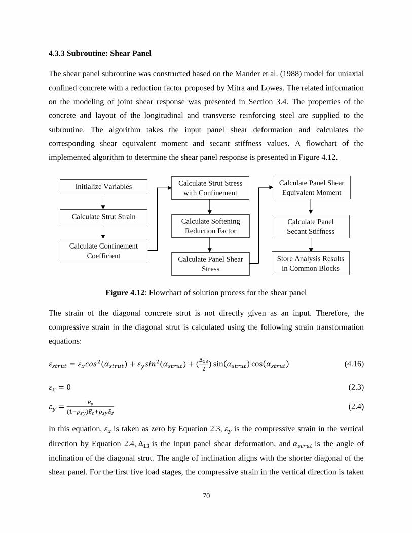
70
4.3.3 Subroutine: Shear Panel
The shear panel subroutine was constructed based on the Mander et al. (1988) model for uniaxial
confined concrete with a reduction factor proposed by Mitra and Lowes. The related information
on the modeling of joint shear response was presented in Section 3.4. The properties of the
concrete and layout of the longitudinal and transverse reinforcing steel are supplied to the
subroutine. The algorithm takes the input panel shear deformation and calculates the
corresponding shear equivalent moment and secant stiffness values. A flowchart of the
implemented algorithm to determine the shear panel response is presented in Figure 4.12.
Figure 4.12: Flowchart of solution process for the shear panel
The strain of the diagonal concrete strut is not directly given as an input. Therefore, the
compressive strain in the diagonal strut is calculated using the following strain transformation
equations:
휀𝑠𝑡𝑟𝑢𝑡 = 휀𝑥𝑐𝑜𝑠2(𝛼𝑠𝑡𝑟𝑢𝑡) + 휀𝑦𝑠𝑖𝑛
2(𝛼𝑠𝑡𝑟𝑢𝑡) + (∆13
2) sin(𝛼𝑠𝑡𝑟𝑢𝑡) cos(𝛼𝑠𝑡𝑟𝑢𝑡) (4.16)
휀𝑥 = 0 (2.3)
휀𝑦 =𝑃𝑣
(1−𝜌𝑠𝑦)𝐸𝑐+𝜌𝑠𝑦𝐸𝑠 (2.4)
In this equation, 휀𝑥 is taken as zero by Equation 2.3, 휀𝑦 is the compressive strain in the vertical
direction by Equation 2.4, ∆13 is the input panel shear deformation, and 𝛼𝑠𝑡𝑟𝑢𝑡 is the angle of
inclination of the diagonal strut. The angle of inclination aligns with the shorter diagonal of the
shear panel. For the first five load stages, the compressive strain in the vertical direction is taken
Initialize Variables
Calculate Strut Strain
Calculate Confinement
Coefficient
Calculate Strut Stress
with Confinement
Calculate Softening
Reduction Factor
Calculate Panel Shear
Stress
Calculate Panel Shear
Equivalent Moment
Calculate Panel
Secant Stiffness
Store Analysis Results
in Common Blocks

71
as zero because the domination of column compression in the early load stages may produce the
undesired result of the stiffness matrix not being positive definite at early load stages.
Mander et al. proposed a theoretical stress-strain model for confined concrete. Figure 4.13
illustrates the stress-strain model for the monotonic loading of confined and unconfined concrete.
It also suggests that the confined concrete fails at the first hoop fracture. This model considers
the fraction of concrete that is confined by the transverse reinforcing steel, and enhances the
strength and ductility of the concrete according to the confinement effectiveness coefficient. The
confined concrete compressive stress 𝑓𝑐𝑐 is given by
𝑓𝑐𝑐 =𝑓𝑐𝑐′ 𝑥𝑟
𝑟−1+𝑥𝑟 (4.17)
𝑤ℎ𝑒𝑟𝑒 𝑥 =𝜀𝑠𝑡𝑟𝑢𝑡
𝜀𝑐𝑐′ (4.18)
𝑎𝑛𝑑 𝑟 =𝐸𝑐
𝐸𝑐−𝐸𝑠𝑒𝑐 (4.19)
where 𝑓𝑐𝑐′ is the compressive strength of confined concrete, parameter 𝑥 is a function of the strut
strain, and parameter 𝑟 is a function of the tangent modulus of elasticity of concrete 𝐸𝑐 and the
secant modulus of elasticity of concrete 𝐸𝑠𝑒𝑐. The tangent modulus is given as an input to the
subroutine. The secant modulus is given by
𝐸𝑠𝑒𝑐 =𝑓𝑐𝑐′
𝜀𝑐𝑐′ (4.20)
where 휀𝑐𝑐′ is the strain at the compressive strength of confined concrete.
Figure 4.13: Stress-strain model for monotonic loading of confined and unconfined concrete
(Mander et al., 1988)

72
Determination of the confined concrete strength and strain requires the consideration of the
effective confinement. Figure 4.14 shows effectively confined concrete in section and elevation
views.
Figure 4.14: Effectively confined concrete for rectangular tie reinforcement (Mander et al., 1988)
The concrete is confined by rectangular ties in the out-of-plane direction, creating a lateral
pressure to stiffen the concrete core. It is assumed that the effective confinement in concrete
diagonal strut equals to the effective confinement of a column segment associated with the
interior joint. The confinement effectiveness coefficient 𝑘𝑒 is given by
𝑘𝑒 =(1−∑
(𝑤𝑖′)2
6𝑏𝑐𝑑𝑐
𝑛𝑖=1 )(1−
𝑠′
2𝑏𝑐)(1−
𝑠′
2𝑑𝑐)
1−𝜌𝑐𝑐 (4.21)
where 𝑛 represents the number of longitudinal bars in the column, 𝜌𝑐𝑐 is the ratio of the
longitudinal reinforcement to area of the confined core section, 𝑤′is the clear distance between
the longitudinal rebars in the column, 𝑠′ is the clear spacing of transverse tie reinforcement, 𝑏𝑐
and 𝑑𝑐 are dimensions to the centerline of the perimeter tie reinforcement in the 𝑥 and 𝑦
directions of the column section, respectively. For joints with no transverse reinforcement or

73
with ineffective transverse reinforcement (i.e. 𝑘𝑒 less than zero), a value of zero is assigned to
the coefficient. Most of the dimensions are determined based on the input geometric parameters.
Because the distance between the longitudinal bars of the same layer is not a required input by
the user, it is assumed to be the inner circumference of the tie divided by the number of
longitudinal bars. Then, the lateral confining stresses in the 𝑥 and 𝑦 directions are calculated as
𝑓𝑙𝑥 = 𝑘𝑒𝜌𝑥𝑓𝑦𝑡 (4.22)
𝑓𝑙𝑦 = 𝑘𝑒𝜌𝑦𝑓𝑦𝑡 (4.23)
where 𝑓𝑦𝑡 is the yield stress of transverse reinforcement, and 𝜌𝑥 and 𝜌𝑦 are the transverse
reinforcing ratios in the 𝑥 and 𝑦 directions of the column section, respectively.
The last step to construct the stress-strain model is to determine the confined concrete strength
𝑓𝑐𝑐′ and corresponding strain 휀𝑐𝑐
′ using the following equations:
𝑓𝑐𝑐′ = 𝑓𝑐
′(−1.254 + 2.254√1 +7.94𝑓𝑙
𝑓𝑐′ + 2
𝑓𝑙
𝑓𝑐′) (4.24)
휀𝑐𝑐′ = 휀𝑐
′ [1 + 5 (𝑓𝑐𝑐′
𝑓𝑐′ − 1)] (4.25)
where 𝑓𝑐′ is the compressive strength of unconfined concrete, 휀𝑐
′ is the strain at compressive
strength, and 𝑓𝑙 is the average confining pressure taken as the average of confining pressure in
the 𝑥 and 𝑦 directions of the column section. The confined concrete strength and strain are
substituted into Equations 4.17 and 4.18 to determine the stress of the confined concrete for a
given strut strain.
The strut stress obtained from the stress-strain model for the confined concrete is multiplied by a
reduction factor accounting for the compression softening effect. The principal tensile and
compressive strains were given by Equation 2.7 and 2.8, respectively.
휀1 =𝜀𝑥+𝜀𝑦
2+√(
𝜀𝑥−𝜀𝑦
2)2 + (
𝛾𝑥𝑦
2)2 (2.7)
휀2 =𝜀𝑥+𝜀𝑦
2−√(
𝜀𝑥−𝜀𝑦
2)2 + (
𝛾𝑥𝑦
2)2 (2.8)

74
The reduction factor was given by Equation 3.12 for joints with transverse reinforcement and
Equation 3.13 for joints without transverse reinforcement.
𝑓𝑐𝑠𝑡𝑟𝑢𝑡
𝑓𝑐𝑀𝑎𝑛𝑑𝑒𝑟= 3.62 |
𝜀𝑡
𝜀𝑐𝑐|2
− 2.82 |𝜀𝑡
𝜀𝑐𝑐| + 1 𝑓𝑜𝑟 |
𝜀𝑡
𝜀𝑐𝑐| < 0.39 (3.12a)
𝑓𝑐𝑠𝑡𝑟𝑢𝑡
𝑓𝑐𝑀𝑎𝑛𝑑𝑒𝑟= 0.45 𝑓𝑜𝑟 |
𝜀𝑡
𝜀𝑐𝑐| ≥ 0.39 (3.12b)
𝑓𝑐𝑠𝑡𝑟𝑢𝑡
𝑓𝑐𝑀𝑎𝑛𝑑𝑒𝑟= 0.36 |
𝜀𝑡
𝜀𝑐𝑐|2
− 0.60 |𝜀𝑡
𝜀𝑐𝑐| + 1 𝑓𝑜𝑟 |
𝜀𝑡
𝜀𝑐𝑐| < 0.83 (3.13a)
𝑓𝑐𝑠𝑡𝑟𝑢𝑡
𝑓𝑐𝑀𝑎𝑛𝑑𝑒𝑟= 0.75 𝑓𝑜𝑟 |
𝜀𝑡
𝜀𝑐𝑐| ≥ 0.83 (3.13b)
Then, the panel shear stress was determined using the obtained strut stress and Equation 3.14.
𝜏𝑠𝑡𝑟𝑢𝑡 = 𝑓𝑐_𝑠𝑡𝑟𝑢𝑡𝑤𝑠𝑡𝑟𝑢𝑡𝑐𝑜𝑠𝛼𝑠𝑡𝑟𝑢𝑡
𝑤= 𝑓𝑐_𝑠𝑡𝑟𝑢𝑡
𝑤𝑠𝑡𝑟𝑢𝑡𝑠𝑖𝑛𝛼𝑠𝑡𝑟𝑢𝑡
ℎ (3.14)
Finally, the shear equivalent moment acting on the joint panel component is calculated as
𝑓13 = 𝜏𝑠𝑡𝑟𝑢𝑡 ∙ 𝑤 ∙ ℎ ∙ 𝑡 (4.26)
where 𝑤, ℎ and 𝑡 are the width, height and thickness of the joint panel, respectively. The secant
stiffness is defined as the shear equivalent moment divided by the panel shear deformation.
At the end of the subroutine, the cracking angle 𝜃𝑐𝑟, the mean crack spacing 𝑠𝑐𝑟, the mean crack
width 𝑤𝑐𝑟, the tie strain 휀𝑠𝑧 and the tie stress 𝑓𝑠𝑧 are calculated as a part of the joint analysis
results in the output files using the following equations:
𝜃𝑐𝑟 = |90° +1
2arctan
2∆13
𝜀𝑥−𝜀𝑦| (4.27)
𝑠𝑐𝑟 =1
cos𝜃
𝑠𝑚𝑥+sin𝜃
𝑠𝑚𝑦
(4.28)
𝑤𝑐𝑟 = 휀1 ∙ 𝑠𝑐𝑟 (4.29)
휀𝑠𝑧 =𝐸𝑐
𝐸𝑐+𝜌𝑧𝐸𝑠𝑧(−0.15
𝑓2
𝜀2) (4.30)
𝑓𝑠𝑧 = 𝐸𝑠 ∙ 휀𝑠𝑧 ≤ 𝑓𝑦𝑧 (4.31)

75
where 𝑠𝑚𝑥 and 𝑠𝑚𝑦 are the mean crack spacing in the 𝑥 and 𝑦 directions of the shear panel, 𝜌𝑧 is
the out-of-plane reinforcing ratio, 𝐸𝑠𝑧 is the modulus of elasticity of the transverse reinforcement,
𝑓𝑦𝑧 is the yield stress of the transverse reinforcement, and all other variables are previously
defined.
4.4 Modifications of the Global Frame Analysis Procedure
In order to integrate the local joint element into the global frame analysis procedure, proper
modifications of the global frame analysis procedure are necessary. There are three components
of the global procedure that requires modifications. The first component is the detection of the
interior joints. Interior joints are detected in the shear protection subroutine, and the relevant
information is stored in the common blocks. The next part is the assembly of the global stiffness
matrix. A revised method is proposed to fit the replacement of the existing beam and column
members in the joint region for the joint elements. Finally, two minor modifications are made in
the main program to facilitate the joint implementation.
4.4.1 Detection of Interior Joints
Detection of interior joints is performed in the shear protection subroutine. The obtained joint
information is also stored in the form of arrays and matrices in the common blocks. The relevant
variables are introduced in Section 4.3.1. In this algorithm, an interior joint node is labelled if
the node is associated with four members. Similarly, an exterior joint node has three members
framing into it, whereas a knee joint node has two members framing into it. The total numbers of
interior, exterior and knee joints are also noted. The joint element algorithm requires input such
as the node numbers that define an interior joint, the member numbers of in-framing members,
and the members in the joint region. The input is sorted into arrays or matrices in the counter-
clockwise direction starting from the bottom. Figure 4.15 shows an example of the interior joint
information stored in the common blocks. The node numbers, for example, are sorted based on
their coordinates. The node with the lowest y coordinate among the four external nodes is
defined as the bottom node. The node with the highest x coordinate is defined as the second node
in the list. The node with the highest y coordinate appears as the third node in the list. The last

76
node is the one with the lowest x coordinate. The member information is also identified and
stored in a similar way.
Figure 4.15: Interior joint information in the common blocks
4.4.2 Assembly of the Global Stiffness Matrix
The method to assemble the global stiffness matrix is modified for the joint element
implementation. In the original algorithm, stiffness matrices for individual members are
assembled into a global stiffness matrix as shown in Figure 4.16a. The implementation omits the
joint nodes and replaces four members in the joint regions with joint elements. The element
stiffness matrices of all interior joints in the structure are stored into a joint analysis matrix with
the same size as the global matrix as shown in Figure 4.16b. Eventually, the joint analysis matrix
is added to the member stiffness matrix for the assembly of the global stiffness as shown in
Figure 4.16c. Because of the omission of the interior joint nodes, the size of the global stiffness
matrix is reduced by a degree of three for each interior joint detected. The size of the load and
the displacement vectors is also adjusted to reflect the removal of the joint nodes.
9 10 11 12 13
26
27
28
29
9 10 11 12 26
27
28
25
Interior Joint Information:
JNTINT (joint node numbers):
27 12 28 10
JMINT (framing member numbers):
25 12 28 9
JMTINTT (joint member numbers):
26 11 27 10
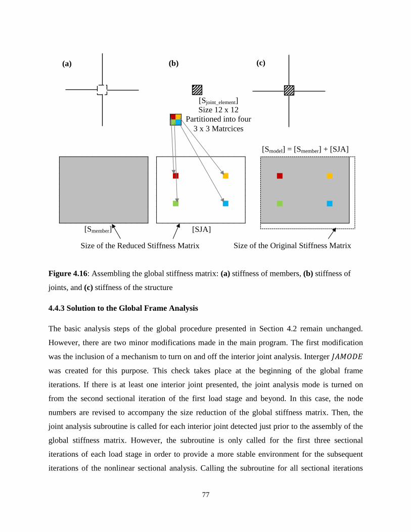
77
Figure 4.16: Assembling the global stiffness matrix: (a) stiffness of members, (b) stiffness of
joints, and (c) stiffness of the structure
4.4.3 Solution to the Global Frame Analysis
The basic analysis steps of the global procedure presented in Section 4.2 remain unchanged.
However, there are two minor modifications made in the main program. The first modification
was the inclusion of a mechanism to turn on and off the interior joint analysis. Interger 𝐽𝐴𝑀𝑂𝐷𝐸
was created for this purpose. This check takes place at the beginning of the global frame
iterations. If there is at least one interior joint presented, the joint analysis mode is turned on
from the second sectional iteration of the first load stage and beyond. In this case, the node
numbers are revised to accompany the size reduction of the global stiffness matrix. Then, the
joint analysis subroutine is called for each interior joint detected just prior to the assembly of the
global stiffness matrix. However, the subroutine is only called for the first three sectional
iterations of each load stage in order to provide a more stable environment for the subsequent
iterations of the nonlinear sectional analysis. Calling the subroutine for all sectional iterations
(a) (b) (c)
[SJA] [Smember]
[Smodel] = [Smember] + [SJA]
[Sjoint_element]
Size 12 x 12
Partitioned into four
3 x 3 Matrcices
Size of the Reduced Stiffness Matrix Size of the Original Stiffness Matrix

78
may result in a constant convergence factor throughout the iterations of a load stage. The second
minor change concerned the unbalanced force. The unbalanced force approach is not applicable
to the joint element because the layered analysis is not performed. The unbalanced forces and the
compatibility restoring forces are set to zero for members in the joint region. This eliminates the
possibility of getting unrealistic convergence factors for those members in the sectional iterations.
4.5 Guidelines for Modeling Beam-Column Joints
The implementation of the joint element requires new guidelines for modeling beam-column
joints in VecTor5. Originally, VecTor5 employed semi-rigid end offsets is to model beam-
column joints in a frame structure. This technique requires doubling the amount of longitudinal
and transverse reinforcing steel for members inside the joint region. The concrete properties
remain unchanged. For the updated VecTor5 considering joint behavior, the interior joints should
be modeled without semi-rigid end offsets, whereas exterior and knee joints should still be
modeled with semi-rigid end offsets. The user should follow the following general guidelines
and assumptions during the process of model creation:
An interior joint should be modeled with two identical beam members and two identical
column members.
The beam members account for the longitudinal reinforcing bars in the 𝑥 direction in the
joint region.
The column members account for the longitudinal reinforcing bars in the 𝑦 direction and
the transverse reinforcement in the joint region.
The longitudinal reinforcing bars with different diameters may be used to construct the
joint model. However, the average diameter of the compression or tension bars is
calculated and used for bar slip spring calculations.
For joints with no transverse reinforcement, the spacing and the reinforcing ratio of
transverse reinforcement should be input as zero.
For joints reinforced with a single set of tie reinforcement, the spacing of transverse
reinforcement is assumed to be half of the joint height.

79
For joints reinforced with multiple sets of tie reinforcement, the spacing provided in the
design is used.
For joints reinforced with a combination of square and diamond orientation of ties, the
area of the transverse reinforcement is assumed to be the sum of the two.
Steel plates and fiber-reinforced polymer composites used as transverse reinforcement are
not considered in the joint analysis.
Members outside the joint regions are modeled using the same technique as before. Additional
information on modeling reinforced concrete frame structures in VecTor5 is available in “User’s
Manual of VecTor5” by Guner and Vecchio (2008).
4.6 Interpretation of Results
Results from the joint analysis are printed in the output files for users to review. This following
section will discuss the layout and content of joint analysis results. This information will be used
to develop a graphical representation in the post-processing program Janus by subsequent
students.
4.6.1 Output Files
VecTor5 stores the analysis results of individual load stages in output files (*.A5E). The results
from interior joint analysis are printed at the end of the output file. The member and joint
analysis results for the members associated with the interior joints are shown in Figure 4.17 and
Figure 4.18, respectively.
Figure 4.17: Layout of member analysis results for members in joint regions
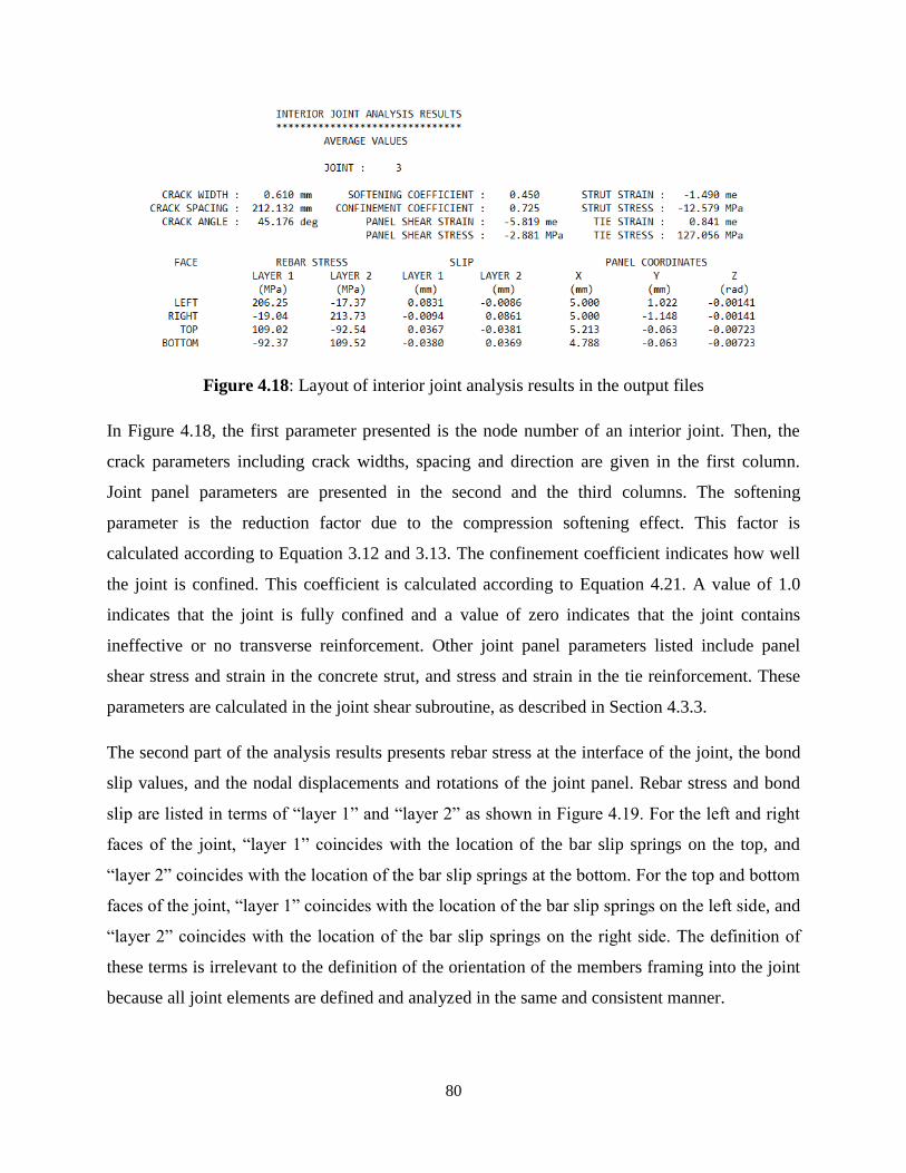
80
Figure 4.18: Layout of interior joint analysis results in the output files
In Figure 4.18, the first parameter presented is the node number of an interior joint. Then, the
crack parameters including crack widths, spacing and direction are given in the first column.
Joint panel parameters are presented in the second and the third columns. The softening
parameter is the reduction factor due to the compression softening effect. This factor is
calculated according to Equation 3.12 and 3.13. The confinement coefficient indicates how well
the joint is confined. This coefficient is calculated according to Equation 4.21. A value of 1.0
indicates that the joint is fully confined and a value of zero indicates that the joint contains
ineffective or no transverse reinforcement. Other joint panel parameters listed include panel
shear stress and strain in the concrete strut, and stress and strain in the tie reinforcement. These
parameters are calculated in the joint shear subroutine, as described in Section 4.3.3.
The second part of the analysis results presents rebar stress at the interface of the joint, the bond
slip values, and the nodal displacements and rotations of the joint panel. Rebar stress and bond
slip are listed in terms of “layer 1” and “layer 2” as shown in Figure 4.19. For the left and right
faces of the joint, “layer 1” coincides with the location of the bar slip springs on the top, and
“layer 2” coincides with the location of the bar slip springs at the bottom. For the top and bottom
faces of the joint, “layer 1” coincides with the location of the bar slip springs on the left side, and
“layer 2” coincides with the location of the bar slip springs on the right side. The definition of
these terms is irrelevant to the definition of the orientation of the members framing into the joint
because all joint elements are defined and analyzed in the same and consistent manner.
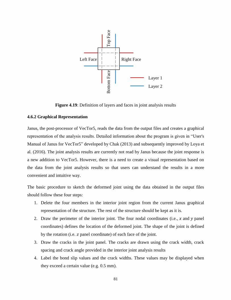
81
Figure 4.19: Definition of layers and faces in joint analysis results
4.6.2 Graphical Representation
Janus, the post-processor of VecTor5, reads the data from the output files and creates a graphical
representation of the analysis results. Detailed information about the program is given in “User's
Manual of Janus for VecTor5” developed by Chak (2013) and subsequently improved by Loya et
al. (2016). The joint analysis results are currently not read by Janus because the joint response is
a new addition to VecTor5. However, there is a need to create a visual representation based on
the data from the joint analysis results so that users can understand the results in a more
convenient and intuitive way.
The basic procedure to sketch the deformed joint using the data obtained in the output files
should follow these four steps:
1. Delete the four members in the interior joint region from the current Janus graphical
representation of the structure. The rest of the structure should be kept as it is.
2. Draw the perimeter of the interior joint. The four nodal coordinates (i.e., 𝑥 and 𝑦 panel
coordinates) defines the location of the deformed joint. The shape of the joint is defined
by the rotation (i.e. 𝑧 panel coordinate) of each face of the joint.
3. Draw the cracks in the joint panel. The cracks are drawn using the crack width, crack
spacing and crack angle provided in the interior joint analysis results
4. Label the bond slip values and the crack widths. These values may be displayed when
they exceed a certain value (e.g. 0.5 mm).
Layer 1
Layer 2
Right Face Left Face
Top F
ace
Bott
om
Fac
e

82
5. The reinforcing bar at the interface of the interior joint may be displayed in a green color
if the yielding stress is reached.
Figure 4.20 illustrates the concept of sketching the deformed interior joint using some sample
values. Components with negative slip are not important for the graphical representation; they
are only used to construct the material model. Meanwhile, for the components with significant
positive slip, an opening at the interface of the joint should be displayed, as it represents cracking
between the interior joint and the members framing into the joint.
Figure 4.20: Sample sketch of a deformed interior joint

83
CHAPTER 5
MODEL EVALUATION AND VERIFICATION
5.1 Chapter Layout
In this chapter, the modified frame analysis procedure VecTor5 with the new joint element is
evaluated and validated with experimental tests of beam-column joint subassemblies and large
reinforced concrete frame structures. Examples and important considerations in modeling the
joint subassemblies and frames are also discussed. The structures considered include: two joint
subassemblies tested by Shiohara and Kusuhara (2007), two joint assemblies tested by Park and
Dai (1988), two joint assemblies tested by Noguchi and Kashiwazaki (1992), three joint
assemblies tested by Attaalla and Agbabian (2004), and three frame structures tested by Xue et al.
(2011), Ghannoum and Moehle (2012), and Pampanin et al. (2007).
The chapter starts with a summary of nine interior beam-column subassemblies modeled using
the analysis procedure with the new joint element. It is then followed by detailed discussions of
each specimen including the experimental setup, analytical modeling, and comparisons of the
experimental and analytical responses. The chapter continues with a parametric study to
investigate the impact of four parameters on the analytical load-displacement response of the test
specimens. The parameters include: loading type, confinement, compression softening, and bond
stress. Finally, three large-scale frame structures from the literature were analyzed. The results
are presented and discussed at the end of this chapter.
5.2 Beam-Column Subassemblies
5.2.1 Summary
In order to assess the performance of VecTor5 with the new joint element, nine interior beam-
column subassemblies from four different tests were selected for evaluation and verification. In

84
this chapter, analyses performed using VecTor5 with the new joint element are referred to with
the name of the joint element subroutine, V5FBCA.
The inputs used for the analyses with V5FBCA and VecTor5 were almost identical. The only
difference was that the semi-rigid end offsets were not used for interior joints in the analysis with
V5FBCA. The analyses with V5FBCA and VecTor5 employed common modeling options. The
V5FBCA and VecTor5 analyses were performed using only the default or typical material
behavior models to assess the capabilities without using special program modifications. Table
5.1 lists the default material behavior models and analysis parameters used in V5FBCA and
VecTor5. One exception of the material behavior model was the concrete compression base
curve. For high strength concrete with compressive strength greater than 42 MPa, Popovics
(HSC) model was employed instead of the default Hognestad parabola model.
Table 5.1: Material behavior models and analysis parameters used in VecTor5
Material Property Model
Concrete Compression Base Curve Popovics – NSC
Concrete Compression Post-Peak Modified Park-Kent
Concrete Compression Softening Vecchio 1992-A
Concrete Tension Stiffening Modified Bentz
Concrete Tension Softening Linear
Concrete Tension Splitting Not Considered
Concrete Confined Strength Kupfer / Richart
Concrete Dilation Variable - Kupfer
Concrete Cracking Criterion Mohr-Coulomb (Stress)
Concrete Crack Width Check Crack Limit (Agg/5)
Concrete Hysteresis NL (Vecchio)
Concrete Slip Distortion Vecchio-Lai
Reinforcement Hysteresis Seckin with Bauschinger
Reinforcement Dowel Action Tassios (Crack Slip)
Reinforcement Buckling Malvar and Crawford
Geometric Nonlinearity Considered
Shear Analysis Mode Parabolic Shear Strain
Shear Protection On
Convergence Limit 1.00001
Maximum Number of Iterations 100
In addition, the response parameters not explicitly calculated in the programs were approximated
based on the following assumptions:

85
In analyses with the original VecTor5 program, bar stresses at the joint interface were
assumed to equal to the bar stresses in the members framing into the joint. Beam and
column members in the joint region were not used because the method of semi-rigid end
offsets significantly reduced the reinforcement stresses in those members.
For joints with multiple layers of longitudinal reinforcing bars, the stresses in the two
extreme layers of steel were used for the comparison.
In the experimental studies, eight subassemblies were subjected to reversed cyclic loading
conditions, and one subassembly was tested under monotonic loading. The analytical study is
focused on the interior beam-column joints subjected to monotonic loading. Therefore, the
specimens were modeled under monotonic loading conditions. Table 5.2 summarizes the
geometric properties and analytical results of nine specimens. These experimental joint
subassemblies exhibited one of the following three failure mechanisms: beam yielding with no
joint failure (BY), joint failure prior to beam yielding (JF), and beam yielding followed by joint
failure (BYJF).
Table 5.2: Summary of the specimen properties and analytical results of interior beam-column
subassemblies
Specimen
Shiohara and Kusuhara
(2007)
Park and Dai
(1988)
A1 D1 U1 U2
(a) Beam Properties
Top Reinforcement
Bottom Reinforcement
Transverse Reinforcement
8-D13
8-D13
D6 @ 50 mm
6-D13
6-D13
D6 @ 50 mm
5-D16
2-D16
various
2-D28
2-D20
various
(b) Column Properties
Longitudinal Reinforcement
Transverse Reinforcement
16-D13
D6 @ 50 mm
14-D13
D6 @ 50 mm
8-D16
various
8-D20
various
(c) Joint Properties
Concrete Strength (MPa)
Height (mm)
Width (mm)
Thickness (mm)
Trans. Reinforcement
Confinement Coefficient
28.3
300
300
300
5-D6
0.725
30.4
300
300
300
5-D6
0.702
45.9
457
406
305
5-D12/D8
0.560
36.0
457
406
305
5-D12
0.570
(d) Results (“Analysis” refers to the results from V5FBCA analysis)
Failure Mechanism Analysis
Experiment
JF
BYJF
JF
BYJF
BY
BY
BY
BY

86
Peak Load
(kN)
Analysis
Experiment
Analysis/Exp.
VT5/Exp.
94.0
126.6
0.74
1.24
112.7
133.9
0.84
1.22
94.7
80.0
1.18
1.18
132.7
111.0
1.20
1.29
Max. Panel Shear Stress
(MPa)
Analysis
Experiment
Analysis/Exp.
3.70
N/A
N/A
4.40
N/A
N/A
3.70
N/A
N/A
4.91
N/A
N/A
Load at First Beam
Yielding
(kN)
Analysis
Experiment
Analysis/Exp.
VT5/Exp.
N/A
118.6
N/A
1.19
N/A
89.7
N/A
1.49
67.6
54.2
1.25
1.32
50.6
78.9
0.64
1.29
Specimen
Noguchi and Kashiwazaki
(1992)
Attaalla and Agbabian
(2004)
OKJ-2 OKJ-6 SHC-1 SHC-2 SOC-3
(a) Beam Properties
Top Reinforcement
Bottom Reinforcement
Transverse Reinforcement
9-D13
7-D13
D6 @ 50 mm
8-D13
7-D13
D6 @ 50 mm
3-D10
3-D10
D6 @ 72 mm
3-D10
3-D10
D6 @ 72 mm
3-D10
3-D10
D6 @ 72 mm
(b) Column Properties
Longitudinal Reinforcement
Transverse Reinforcement
20-D13
D6 @ 40 mm
20-D13
D6 @ 40 mm
4-D13
D6 @ 51 mm
4-D13
D6 @ 51 mm
4-D13
D6 @ 51 mm
(c) Joint Properties
Concrete Strength (MPa)
Height (mm)
Width (mm)
Thickness (mm)
Transverse Reinforcement
Confinement Coefficient
70.0
300
300
300
6-D6
0.786
53.5
300
300
300
6-D6
0.786
56.5
203
178
127
1-D6
0.102
59.5
203
178
127
2-D6
0.189
47.2
203
178
127
2-D6
0.187
(d) Results (“Analysis” refers to the results from V5FBCA analysis)
Failure
Mechanism
Analysis
Experiment
BY
BYJF
BY
JF
BYJF
BYJF
BYJF
BYJF
BYJF
BYJF
Peak Load
(kN)
Analysis
Experiment
Analysis/Exp
VT5/Exp.
265.6
237.0
1.12
1.16
264.2
214.0
1.23
1.25
16.38
16.02
1.02
1.34
18.36
16.73
1.10
1.29
15.65
16.02
0.94
1.26
Max. Panel
Shear Stress
(MPa)
Analysis
Experiment
Analysis/Exp
12.81
14.16
0.90
11.53
13.11
0.88
5.21
6.88
0.76
5.80
7.24
0.80
4.87
7.20
0.68
Load at First
Beam Yielding
(kN)
Analysis
Experiment
Analysis/Exp
VT5/Exp.
245.9
237
1.04
1.02
248.2
N/A
N/A
N/A
15.91
11.90
1.34
1.30
15.59
12.20
1.30
1.32
15.47
13.40
1.15
1.20
Mean
(Analysis/Exp)
Peak Load
Max. Panel Shear Stress
Load at First Beam Yielding
1.05 (9 specimens)
0.80 (5 specimens)
1.12 (6 specimens)
Coefficient of
Variation (%)
Peak Load
Max. Panel Shear Stress
Load at First Beam Yielding
16.3 (9 specimens)
11.2 (5 specimens)
23.1 (6 specimens)

87
Mean
(VT5/Exp)
Peak Load
Load at First Beam Yielding
1.25 (9 specimens)
1.27 (8 specimens)
VT5 Coefficient
of Variation (%)
Peak Load
Load at First Beam Yielding
4.5 (9 specimens)
10.7 (8 specimens)
With the new joint element, VecTor5 was able to provide better predictions in terms of failure
mechanism and peak loads. For the nine interior joint subassemblies modeled, the ratio of
predicted and observed peak load had a mean of 1.06 and a coefficient of variation of 18.3%. For
the six specimens that exhibit beam yielding, the ratio of predicted and observed load at first
beam yielding had a mean of 1.09 and a coefficient of variation of 21.5%.
5.2.2 Shiohara and Kusuhara (2007)
The first set of subassemblies modeled was from a benchmark test conducted by Shiohara and
Kusuhara at the University of Tokyo in Japan. Six half-scaled reinforced concrete beam-column
joint subassemblies isolated from moment resisting frames were tested. These specimens were
seismically designed according to the AIJ Guidelines (1999). Specimen A1 was selected for this
verification study. Other specimens were excluded because they were either exterior or knee
joints. Shiohara and Kusuhara presented the test results of four additional specimens with similar
experimental setup in their subsequent study (Shiohara and Kusuhara, 2008). Specimen D1 was
selected as the second specimen for the verification.
5.2.2.1 Test Specimens
Specimens A1 and D1 had identical overall dimensions, loading setup and support restraints, but
the sectional and material properties were slightly different. Figure 5.1 shows the test setup, and
Figure 5.2 shows the sectional details of Specimens A1 and D1. All beam and column sections
were 300 by 300 mm. The joint panel was reinforced with three transverse hoops. To measure
the post-yielding stress and strain in the longitudinal reinforcing bar in the specimens, a box
shape groove was made on two sides of each bar for the installation of strain gauges. The
location of the grooved longitudinal bars in the beam sections is indicated by solid dots in Figure
5.2. The cross-sectional area of grooved bars was 75% of the original cross-sectional area. These
bars were used inside the joint panel as well as in the beam at the locations within 450 mm from

88
the face of the column. The material properties of the concrete and the reinforcement are listed in
Table 5.3. The subassemblies were loaded by a displacement-based horizontal reversed cyclic
load, and a constant axial load of 216 kN was applied at the top of the column. A pin support was
provided at the bottom of the column, and a roller was provided at both ends of the beam. This
test setup was used to simulate a typical boundary condition of an interior joint.
Figure 5.1: Test setup of Specimens A1 and D1 (adapted from Guner, 2008)
Table 5.3: Material properties of Specimens A1 and D1
Bar
Type
Reinforcement Properties
db
(mm)
Fy
(MPa)
Fu
(MPa)
Es
(MPa)
Esh
(MPa)
εsh
(x10-3
)
εu
(x10-3
)
D13B1 12.7 456 582 176000 952 27.6 160
D13C1 12.7 357 493 176000 1032 28.2 160
D61 6.4 326 388 151000 5391 4.2 15.7
D16B2 16.0 379 558 187000 1352 27.6 160
D13C2 12.7 375 538 187000 1237 28.2 160
D62 6.4 366 504 191000 12000 4.2 15.7
Spec.
Concrete Properties
f’c
(MPa)
f’t
(MPa)
Ec
(MPa)
ε’c
(x10-3
)
A1 28.3 1.76 25900 1.87
D1 30.4 1.82 30000 2.03
1: Used in Specimen A1
2: Used in Specimen D1

89
Figure 5.2: Sectional details of Specimens A1 and D1
5.2.2.2 Analytical Modeling
The two subassemblies were modeled using the same structural model, loading type and
boundary conditions. The details and material properties of members were slightly different.
Figure 5.3 shows the analytical model with dimensions, loading and support restraints. There
were 37 nodes, 36 members and 4 support restraints in the model. The support conditions
included restraints of the horizontal and vertical translations at Node 26 and restraint of the
vertical translation at Node 1 and Node 25. An axial compressive load of 216 kN was applied at
Node 37. A positive displacement at Node 37 was applied in 81 load stages with an increment of
1 mm starting from a zero displacement.
A1 Beam Section D1 Beam Section
A1 Column Section D1 Column Section

90
Figure 5.3: Analytical model showing dimensions, loading and support restraints of Specimens
A1 and D1
Five member types were created to build the model (see Figure 5.4). The beam sections near the
roller supports were represented by Member Type 1 (MT1) whereas the beam sections near the
column were represented by MT2 accounting for the grooved bars. The column sections were
represented by MT3. The interior joint was modeled by MT2 in the horizontal direction and MT3
in the vertical direction. MT4 and MT5 were created by doubling the reinforcing ratios of MT2
and MT3, respectively, to simulate the relatively stiffer response of the joint panel. MT4 and
MT5 were only used in the analysis with the original VecTor5 program for the purpose of
comparing the responses obtained prior and after the joint implementation. Each member was
divided into 18 concrete layers to perform the sectional fiber analysis. Detailed general and
sectional material properties of Specimen A1 are presented in Tables 5.4, 5.5 and 5.6. Specimen
D1 was modeled using a similar approach.
For VecTor5 modeling of beam-column joint subassemblies, it is recommended to use at least 30
layers for the concrete sections. Layers at the top and bottom of the section should be finer than
the ones at the centroid and the neutral axis. This refinement, which is valid for all the specimens
modeled in this study, may further improve the analytical results.
216 kN
750 750 450 450 150 150
58
5
58
5
15
0
Displacement
(+1 mm)

91
Figure 5.4: Analytical model showing material types of Specimens A1 and D1
Table 5.4: General material specifications of Specimen A1
MT
Concrete Properties Transverse Reinforcement Properties
f’c
(MPa)
f’t
(MPa)
Ec
(MPa)
ε’c
(x10-3
) Other
st
(mm)
dbt
(mm)
Fyt
(MPa)
Fut
(MPa)
Est
(MPa)
εsht
(x10-3
)
εut
(x10-3
)
1-5 28.3 1.76 25900 1.87 default 50.0 6.4 326 388 151000 4.2 15.7
Table 5.5: Reinforced concrete material specifications of Specimen A1
MT Dc
(mm)
Wc
(mm)
ρt
(%)
ρz
(%) Nx MT
Dc
(mm)
Wc
(mm)
ρt
(%)
ρz
(%) Nx
1
22.00
300
0.000 0.876 1
4
22.00
300
0.000 1.752 1
17.02 0.427 0.876 3 17.02 0.854 1.752 3
15.39 0.427 0.000 5 15.39 0.854 0.000 5
15.39 0.427 0.000 5 15.39 0.854 0.000 5
17.02 0.427 0.876 3 17.02 0.854 1.752 3
22.00 0.000 0.876 1 22.00 0.000 1.752 1
2
22.00
300
0.000 0.876 1
5
22.00
300
0.000 1.752 1
17.02 0.427 0.876 3 17.02 0.854 1.752 3
15.39 0.427 0.000 5 15.39 0.854 0.000 5
15.39 0.427 0.000 5 15.39 0.854 0.000 5
17.02 0.427 0.876 3 17.02 0.854 1.752 3
22.00 0.000 0.876 1 22.00 0.000 1.752 1
3
22.00
300
0.000 0.876 1 MT: Member Type
17.02 0.427 0.876 3 Dc: Layer Depth
15.39 0.427 0.000 5 Wc: Width of the Section
15.39 0.427 0.000 5 ρt: Transverse Reinforcing Ratio
17.02 0.427 0.876 3 ρz: Out-of-Plane Reinforcing Ratio
22.00 0.000 0.876 1 Nx: Number of Layers
MT1 MT1 MT2 MT2
MT
3
MT
3
MT3
(MT5)
MT2 (MT4)

92
Table 5.6: Longitudinal reinforcement material specifications of Specimen A1
MT N Ys
(mm)
As
(mm2)
Db
(mm)
Fy
(MPa)
Fu
(MPa)
Es
(MPa)
εsh
(x10-3
)
εu
(x10-3
)
1
1 35 508
12.7 456 582 176000 27.6 160 2 70 508
3 230 508
4 265 508
2
1 35 446
11.9 456 582 176000 27.6 160 2 70 446
3 230 446
4 265 446
3
1 35 635
12.7 357 493 176000 28.2 160
2 85 254
3 150 254
4 215 254
5 265 635
4
1 35 892
11.9 456 582 176000 27.6 160 2 70 892
3 230 892
4 265 892
5
1 35 1270
12.7 357 493 176000 28.2 160
2 85 508
3 150 508
4 215 508
5 265 1270
5.2.2.3 Comparison of the Analytical and Experimental Responses
Specimen A1
Specimens A1 and D1 were analyzed with V5FBCA and VecTor5. A comparison of the lateral
load-deflection responses at the column tip is given in Figure 5.5. Detailed comparisons of the
response parameters are reported in Table 5.7.
Table 5.7: Comparison of experimental and analytical results of Specimen A1
Experiment V5FBCA VecTor5
Failure Mechanism BYJF JF BY
Peak Load (kN)
(Ratio = Analysis/Experiment)
126.6
94.0
(0.74)
157.6
(1.24)
Max. Panel Shear Stress (MPa)
(Ratio = Analysis/Experiment)
N/A
3.70
(N/A)
N/A
(N/A)
Load at First Beam Yielding (kN)
(Ratio = Analysis/Experiment)
118.6
N/A
(N/A)
140.7
(1.19)

93
Figure 5.5: Comparison of the load-displacement response of Specimen A1
In the experiment, the beam yielded at a displacement of 21 mm, where the face rotation of the
joint panel suddenly increased, greatly contributing to the overall displacement of the
subassembly. At a displacement of 29 mm, the concrete crushed at the beam-joint interface, and
the concrete cover started spalling off from the joint panel. At a displacement of 44 mm, the
concrete cover spalled off thoroughly, which exposed the ties. Figure 5.6a shows the joint panel
condition at a displacement of 60 mm.
As observed from Figure 5.5, VecTor5 overestimated the stiffness and strength of the
subassembly by 24%. V5FBCA, on the other hand, underestimated the strength of the
subassembly by 26%, but the stiffness and the shape of the response curve were predicted better.
V5FBCA predicted a joint failure without yielding of the beam reinforcement, whereas the
specimen exhibited a failure mechanism of beam yielding followed by joint failure in the
experiment. The shear panel reached its peak stress of 3.70 MPa at a displacement of 26 mm,
when the subassembly reached its peak load of 93.2 kN. The average crack width in the joint
panel at a displacement of 60 mm was determined as 5.5 mm.
-150
-100
-50
0
50
100
150
200
-80 -60 -40 -20 0 20 40 60 80
Load
(k
N)
Displacement (mm)
Experiment
V5FBCA
VecTor5

94
On the contrary, VecTor5 predicted failure due to beam yielding. VecTor5 predicted beam
yielding at the joint interface at a displacement of 13 mm. Flexural cracks initiated in Members
11 and 14 propagated with increasing applied displacement. Cracking in the joint panel was
relatively insignificant (see Figure 5.6b).
Figure 5.6: Cracking pattern of Specimen A1: (a) observed (Shiohara and Kusuhara, 2007) and
(b) original VecTor5 simulation
Overall, neither of the predictions was a good match with the experimental response. V5FBCA
provided a slightly better prediction by identifying the joint failure and the subsequent loss of
stiffness. V5FBCA also provided a good prediction on the concrete response of the joint core.
Two relationships obtained from the analysis were compared to the experimental results. Lateral
load versus shear strain of the joint panel was the first relationship for the evaluation. Figure 5.7
shows the relationship from the experimental response envelope and the monotonic analysis. The
analytical response presented a lower shear strain of 26.4 x 10⁻³
than the experimental shear
strain of 31.8 x 10⁻³
at a displacement of 60 mm. The load from the analysis was lower than that
from the experiment because of the underestimation of the strength of the subassembly.
(a) (b)

95
Figure 5.7: Load versus joint shear strain relationship of Specimen A1
The second parameter for evaluation was the stress in the longitudinal reinforcement. The
stresses obtained from the analysis were compared to those obtained from VecTor5 (see Table
5.8). The stresses in the extreme layer of bars of the beam and column sections were selected for
this comparison because they represented the extreme values of reinforcement stress in the
section. V5FBCA was capable of predicting both tensile and compressive stresses reasonably
well. The stress prediction followed a monotonic trend up to the peak load. One exception was
that yielding of the beam bars was not captured by V5FBCA because of the low global
prediction of the load-displacement response.
0
20
40
60
80
100
120
140
0 5 10 15 20 25 30 35
Load
(k
N)
Shear Strain of Joint Panel (x10-3 rad)
Experiment (envelope)
V5FBCA

96
Table 5.8: Stress in the longitudinal bars at the joint panel interface of Specimen A1
Rebar Stress (MPa)
Disp.
Bottom Face
Compression Side
Bottom Face
Tension Side
Right Face
Tension Side
Right Face
Compression Side
V5FBCA VT5 V5FBCA VT5 V5FBCA VT5 V5FBCA VT5
2 -43 -39 -48 2 55 61 -6 -27
4 -57 -58 -3 24 100 135 -10 -40
6 -72 -77 43 57 145 198 -13 -50
8 -81 -95 73 93 176 250 -16 -60
10 -89 -111 99 130 202 260 -18 -70
12 -95 -127 119 166 224 380 -19 -79
14 -100 -140 136 198 241 456 -21 -83
16 -104 -145 148 214 255 456 -22 -80
20 -108 -147 164 218 272 456 -23 -60
25 -110 -148 170 221 280 456 -24 -39
30 -108 -150 168 226 282 456 -25 -28
40 -104 -153 157 235 283 457 -27 -16
50 -98 -167 145 298 285 476 -30 -12
60 -93 -178 135 353 293 496 -34 -2
Specimen D1
A comparison of the lateral load-deflection responses at the column tip is given in Figure 5.8.
The detailed comparisons of the response parameters are reported in Table 5.9.
Figure 5.8: Comparison of the load-displacement response of Specimen D1
-150
-100
-50
0
50
100
150
200
-80 -60 -40 -20 0 20 40 60 80
Lo
ad
(k
N)
Displacement (mm)
Experiment
V5FBCA
VecTor5
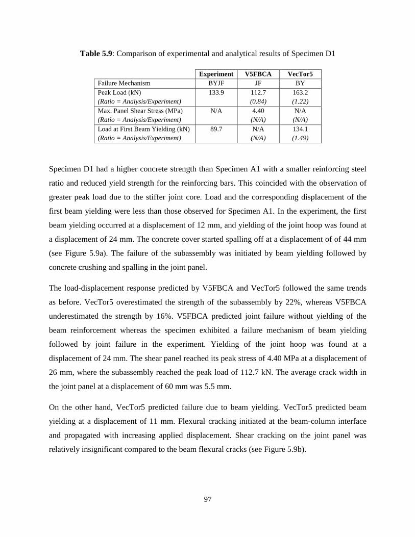
97
Table 5.9: Comparison of experimental and analytical results of Specimen D1
Experiment V5FBCA VecTor5
Failure Mechanism BYJF JF BY
Peak Load (kN)
(Ratio = Analysis/Experiment)
133.9
112.7
(0.84)
163.2
(1.22)
Max. Panel Shear Stress (MPa)
(Ratio = Analysis/Experiment)
N/A
4.40
(N/A)
N/A
(N/A)
Load at First Beam Yielding (kN)
(Ratio = Analysis/Experiment)
89.7
N/A
(N/A)
134.1
(1.49)
Specimen D1 had a higher concrete strength than Specimen A1 with a smaller reinforcing steel
ratio and reduced yield strength for the reinforcing bars. This coincided with the observation of
greater peak load due to the stiffer joint core. Load and the corresponding displacement of the
first beam yielding were less than those observed for Specimen A1. In the experiment, the first
beam yielding occurred at a displacement of 12 mm, and yielding of the joint hoop was found at
a displacement of 24 mm. The concrete cover started spalling off at a displacement of of 44 mm
(see Figure 5.9a). The failure of the subassembly was initiated by beam yielding followed by
concrete crushing and spalling in the joint panel.
The load-displacement response predicted by V5FBCA and VecTor5 followed the same trends
as before. VecTor5 overestimated the strength of the subassembly by 22%, whereas V5FBCA
underestimated the strength by 16%. V5FBCA predicted joint failure without yielding of the
beam reinforcement whereas the specimen exhibited a failure mechanism of beam yielding
followed by joint failure in the experiment. Yielding of the joint hoop was found at a
displacement of 24 mm. The shear panel reached its peak stress of 4.40 MPa at a displacement of
26 mm, where the subassembly reached the peak load of 112.7 kN. The average crack width in
the joint panel at a displacement of 60 mm was 5.5 mm.
On the other hand, VecTor5 predicted failure due to beam yielding. VecTor5 predicted beam
yielding at a displacement of 11 mm. Flexural cracking initiated at the beam-column interface
and propagated with increasing applied displacement. Shear cracking on the joint panel was
relatively insignificant compared to the beam flexural cracks (see Figure 5.9b).

98
Overall, the prediction of the load-displacement response of Specimen D1 was better than that of
Specimen A1. V5FBCA provided a slightly better prediction than VecTor5 by identifying the
joint failure and the subsequent loss of stiffness.
Figure 5.9: Cracking pattern of Specimen D1: (a) observed (Shiohara and Kusuhara, 2008) and
(b) original VecTor5 simulation
5.2.3 Park and Dai (1988)
The second set of subassemblies modeled was from tests conducted by Park and Dai. Four
interior beam-column subassemblies were tested under reversed cyclic and gravity loading.
These specimens were designed following the requirements of the New Zealand concrete design
code, NZS 3101. Plastic hinging was designed to take place in the beams. Two out of the four
interior joint subassemblies, Unit 1 and Unit 2, were selected for verification. The other two
specimens were excluded because they presented only slightly different concrete strength and
reinforcing details from the selected specimens.
5.2.3.1 Test Specimens
Specimens Unit 1 and Unit 2 had identical dimensions, loading setup and support restraints, but
the magnitudes of the applied gravity loads were different. The two subassemblies used different
sectional designs with different concrete and reinforcing steel material properties. Figure 5.10
and Figure 5.11 shows the test setup. Figure 5.12 shows sectional details of Unit 1 and Unit 2.
The beams were 457 by 229 mm, and the columns were 406 by 305 mm. Note that the part of the
(a) (b)

99
column section was reinforced using ties with a combination of square and diamond orientation.
The spacing and type of transverse reinforcement varied along the length of the beams and
columns. The joint was reinforced with five transverse ties in both subassemblies. The material
properties of the concrete and the reinforcement are listed in Table 5.10. The subassemblies were
loaded in a displacement-controlled mode. A pair of gravity loads of 55 kN and 67 kN were
applied at 848 mm away from the column centerlines of Specimens Unit 1 and Unit 2,
respectively. The displacement-based horizontal reversed cyclic load was applied at the top of
the column. The subassemblies were supported by a pin at the bottom of the column. The
supports at both ends of the beam restricted movement in the vertical direction. This setup was
used to simulate a typical boundary condition of an interior joint.
Figure 5.10: Test setup of Specimen Unit 1 (Park and Dai, 1988)
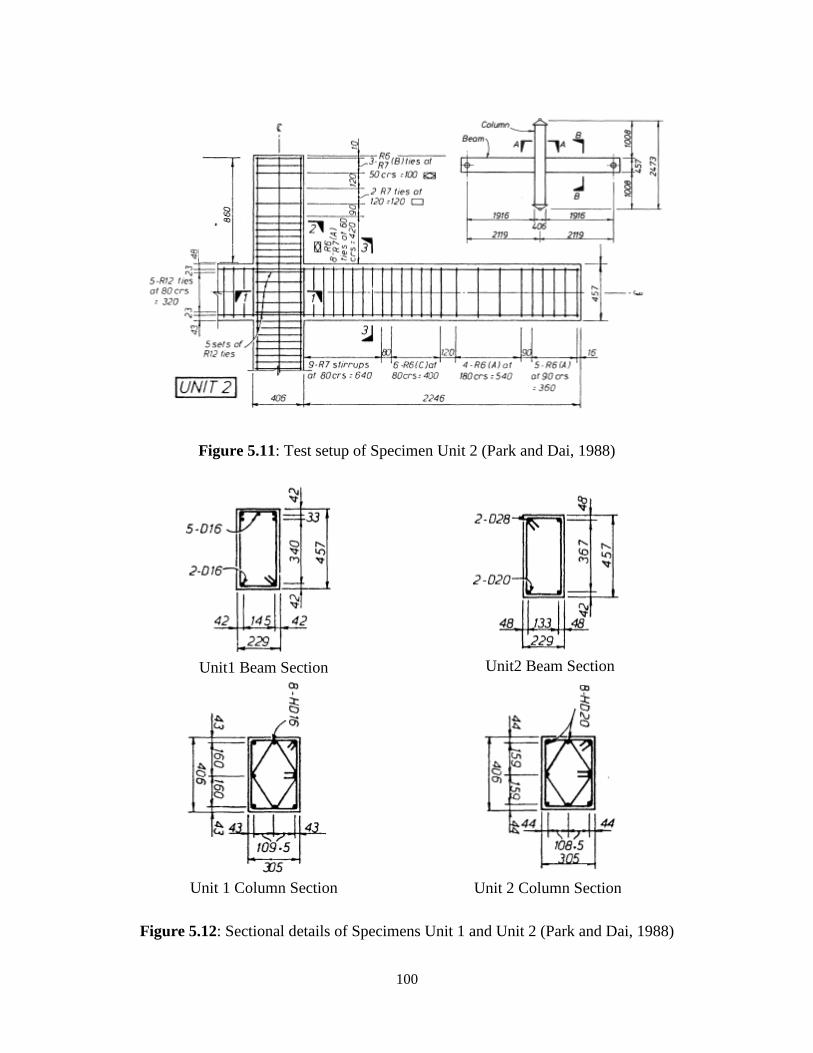
100
Figure 5.11: Test setup of Specimen Unit 2 (Park and Dai, 1988)
Figure 5.12: Sectional details of Specimens Unit 1 and Unit 2 (Park and Dai, 1988)
Unit1 Beam Section Unit2 Beam Section
Unit 1 Column Section Unit 2 Column Section

101
Table 5.10: Material properties of Specimens Unit 1 and Unit 2
5.2.3.2 Analytical Modeling
The subassemblies were modeled using the same structural model and boundary conditions, but
with different loading and sectional properties. Figure 5.13 shows the analytical model with
dimensions, loading, and support restraints. There were 37 nodes, 36 members, and 4 support
restraints in the model. Node 26 was restrained in both the horizontal and vertical directions for a
pin support, while Nodes 1 and 25 were restrained in the vertical direction for roller supports.
Gravity loads of 55 kN were applied at Nodes 8 and 18 of Unit 1. Gravity loads of 67 kN were
applied at the same nodes for Unit 2. A positive horizontal displacement at Node 37 was applied
in 81 load stages with an increment of 2 mm starting from a zero displacement.
Bar
Type
Reinforcement Properties
db
(mm)
Fy
(MPa)
Fu
(MPa)
Es
(MPa)
Esh
(MPa)
εsh
(x10-3
)
εu
(x10-3
)
D16B1 16.0 294 434 210400 3580 25.5 64.6
HD16C1 16.0 498 660 196600 3051 18.0 71.1
D28B2 28.0 314 482 200700 4260 19.3 58.7
D20B2 20.0 300 447 210300 3522 23.8 65.5
HD20C2 20.0 476 644 197100 2800 18.0 78.0
R6(A)1,2
6.0 282 403 205800 1453 5.0 88.3
R6(B)1 6.0 366 466 203400 1541 5.0 69.9
R6(C)2 6.0 360 445 202400 1123 5.0 80.7
R72 7.0 364 521 201100 2133 5.0 78.6
R82 8.0 360 492 189300 1760 5.0 80.0
R121,2
12.0 283 420 202700 1930 5.0 76.0
Spec.
Concrete Properties
f’c
(MPa)
f’t*
(MPa)
Ec*
(MPa)
ε’c*
(x10-3
)
Unit 1 45.9 2.24 29400 2.14
Unit 2 36.0 1.98 26820 2.07
1: Used in Specimen Unit 1
2: Used in Specimen Unit 2
*: estimated
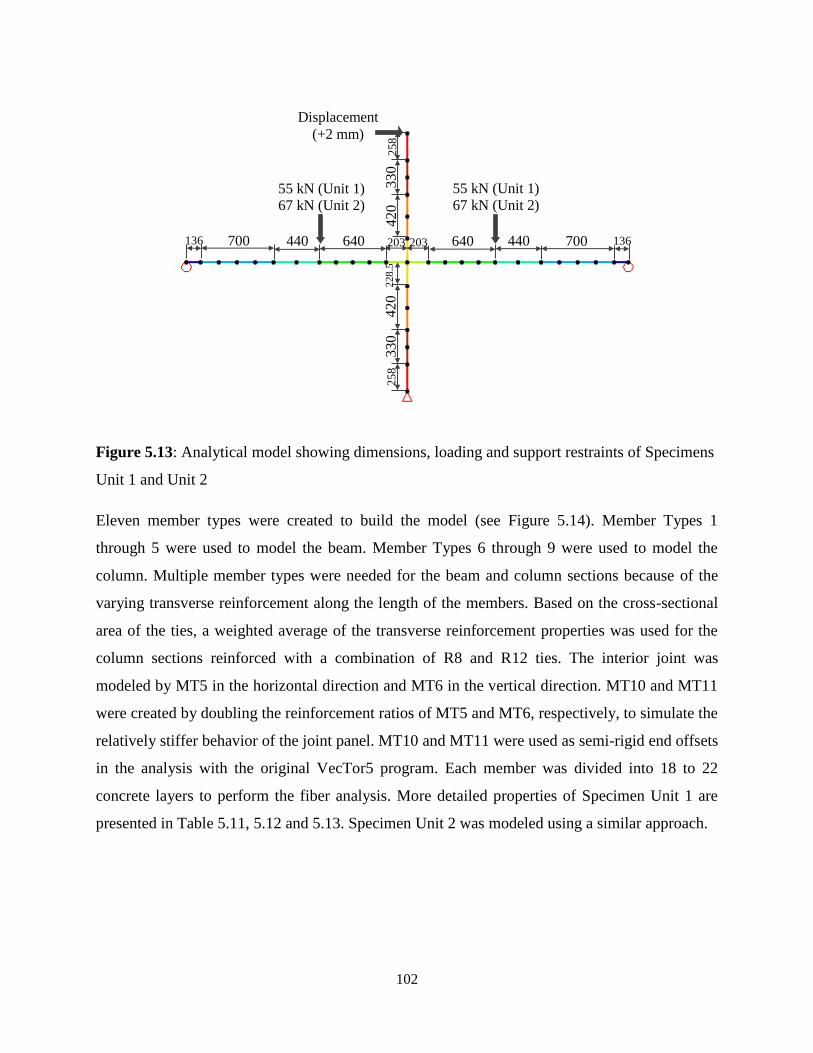
102
Figure 5.13: Analytical model showing dimensions, loading and support restraints of Specimens
Unit 1 and Unit 2
Eleven member types were created to build the model (see Figure 5.14). Member Types 1
through 5 were used to model the beam. Member Types 6 through 9 were used to model the
column. Multiple member types were needed for the beam and column sections because of the
varying transverse reinforcement along the length of the members. Based on the cross-sectional
area of the ties, a weighted average of the transverse reinforcement properties was used for the
column sections reinforced with a combination of R8 and R12 ties. The interior joint was
modeled by MT5 in the horizontal direction and MT6 in the vertical direction. MT10 and MT11
were created by doubling the reinforcement ratios of MT5 and MT6, respectively, to simulate the
relatively stiffer behavior of the joint panel. MT10 and MT11 were used as semi-rigid end offsets
in the analysis with the original VecTor5 program. Each member was divided into 18 to 22
concrete layers to perform the fiber analysis. More detailed properties of Specimen Unit 1 are
presented in Table 5.11, 5.12 and 5.13. Specimen Unit 2 was modeled using a similar approach.
55 kN (Unit 1)
67 kN (Unit 2)
700 700 640 640 203 203
42
0
228
.5
136 136 440 440
330
25
8
25
8
33
0
42
0
55 kN (Unit 1) 67 kN (Unit 2)
Displacement
(+2 mm)

103
Figure 5.14: Analytical model showing material types of Specimens Unit 1 and Unit 2
Table 5.11: General material specifications of Specimen Unit 1
MT
Concrete Properties Transverse Reinforcement Properties
f’c
(MPa)
f’t
(MPa)
Ec
(MPa)
ε’c
(x10-3
) Other
st
(mm)
dbt
(mm)
Fyt
(MPa)
Fut
(MPa)
Est
(MPa)
εsht
(x10-3
)
εut
(x10-3
) 1
45.9 2.24 29400 2.14 default
90 6.0 282 403 205800 5.0 88.3
2 180 6.0 282 403 205800 5.0 88.3
3 110 6.0 366 466 203400 5.0 69.9
4 80 6.0 366 466 203400 5.0 69.9
5 0 0 0 -- -- -- --
6 75 14.4 283 420 202700 5.0 76.0
7 60 8.5 282 403 205800 5.0 88.3
8 120 6.0 366 466 203400 5.0 69.9
9 50 8.5 366 466 203400 5.0 69.9
10 0 0 0 -- -- -- --
11 75 14.4 283 420 202700 5.0 76.0
Table 5.12: Reinforced concrete material specifications of Specimen Unit 1
MT Dc
(mm)
Wc
(mm)
ρt
(%)
ρz
(%) Nx MT
Dc
(mm)
Wc
(mm)
ρt
(%)
ρz
(%) Nx
1
28.00
229
0.000 0.414 1
7
27.00
305
0.000 0.990 1
24.01 0.275 0.414 2 20.41 0.610 0.990 3
19.06 0.275 0.000 8 19.13 0.610 0.000 6
19.06 0.275 0.000 8 19.13 0.610 0.000 6
24.01 0.275 0.414 2 20.41 0.610 0.990 3
28.00 0.000 0.414 1 27.00 0.000 0.990 1
MT2 MT4 MT4
MT
7
MT1 MT1 MT3 MT3
MT
8
MT
9
MT
9
MT
8
MT
7
MT2
MT6 (MT11)
MT5 (MT10)

104
2
28.00
229
0.000 0.213 1
8
27.00
305
0.000 0.310 1
24.01 0.141 0.213 2 24.01 0.160 0.310 2
19.06 0.141 0.000 8 21.33 0.160 0.000 6
19.06 0.141 0.000 8 21.33 0.160 0.000 6
24.01 0.141 0.213 2 24.01 0.160 0.310 2
28.00 0.000 0.213 1 27.00 0.000 0.310 1
3
28.00
229
0.000 0.338 1
9
27.00
305
0.000 1.190 1
24.01 0.225 0.338 2 20.41 0.730 1.190 3
19.06 0.225 0.000 8 19.13 0.730 0.000 6
19.06 0.225 0.000 8 19.13 0.730 0.000 6
24.01 0.225 0.338 2 20.41 0.730 1.190 3
28.00 0.000 0.338 1 27.00 0.000 1.190 1
4
28.00
229
0.000 0.465 1
10
28.00
229
0.000 0.000 1
24.01 0.309 0.465 2 20.05 0.000 0.000 10
19.06 0.309 0.000 8 20.05 0.000 0.000 10
19.06 0.309 0.000 8 28.00 0.000 0.000 1
24.01 0.309 0.465 2
11
19.50
305
0.000 3.240 1
28.00 0.000 0.465 1 21.74 2.860 3.240 5
5
28.00
229
0.000 0.000 1 18.70 2.860 0.000 4
20.05 0.000 0.000 10 18.70 2.860 0.000 4
20.05 0.000 0.000 10 21.74 2.860 3.240 5
28.00 0.000 0.000 1 19.50 0.000 3.240 1
6
19.50
305
0.000 1.620 1
21.74 1.430 1.620 5
18.70 1.430 0.000 4
18.70 1.430 0.000 4
21.74 1.430 1.620 5
19.50 0.000 1.620 1
Table 5.13: Longitudinal reinforcement material specifications of Specimen Unit 1
MT N Ys
(mm)
As
(mm2)
Db
(mm)
Fy
(MPa)
Fu
(MPa)
Es
(MPa)
εsh
(x10-3
)
εu
(x10-3
)
1-5
1 42 600
16.0 294 434 210400 25.5 64.6 2 75 400
3 415 400
6-9
1 43 600
16.0 498 660 196600 18.0 71.1 2 203 400
3 363 600
10
1 42 1200
16.0 294 434 210400 25.5 64.6 2 75 800
3 415 800
11
1 43 1200
16.0 498 660 196600 18.0 71.1 2 203 800
3 363 1200

105
5.2.3.3 Comparison of the Analytical and Experimental Responses
Specimen Unit 1
Specimen Unit 1 was analyzed with V5FBCA and VecTor5. A comparison of the lateral load-
deflection responses at the column tip is given in Figure 5.15. Detailed comparisons of the
response parameters are reported in Table 5.14.
Figure 5.15: Comparison of the load-displacement response of Specimen Unit 1
Table 5.14: Comparison of experimental and analytical results of Specimen Unit 1
Experiment V5FBCA VecTor5
Failure Mechanism BY BY BY
Peak Load (kN)
(Ratio = Analysis/Experiment)
80.2
94.7
(1.18)
95.0
(1.18)
Max. Panel Shear Stress (MPa)
(Ratio = Analysis/Experiment)
N/A
3.73
(N/A)
N/A
(N/A)
Load at First Beam Yielding (kN)
(Ratio = Analysis/Experiment)
54.2
67.6
(1.25)
71.4
(1.32)
-90
-60
-30
0
30
60
90
120
-120 -90 -60 -30 0 30 60 90 120
Late
ral
Load
(k
N)
Displacement (mm)
Experiment
V5FBCA
VecTor5

106
The subassembly was designed for plastic hinging to take place in the beams. The joint panel
was designed with sufficient transverse reinforcement to avoid excessive joint damage. In the
experiment, the subassembly failed due to excessive flexural cracking in the region adjacent to
the column faces. The subassembly sustained its strength and stiffness throughout the test. The
first plastic hinge was formed when the lateral load was 54.2 kN. At a displacement of 30 mm,
the maximum crack width measured was 1.8 mm in the beam, and 0.2 mm in the joint core. The
first cover concrete spalling, occurring on the beam, was observed at a displacement of 45 mm,
when the maximum crack width on the joint panel was found to be 0.6 mm. The hoops in the
joint core reached the yielding stress at the end of the test. Figure 5.16a shows the joint panel
condition at a displacement of 102 mm.
The failure mode predicted by the analysis procedures was flexural failure due to beam yielding.
This prediction matched well with the observed failure mechanism. The analysis results from
V5FBCA were found to be similar to the results from VecTor5 because the response was
governed by yielding of the beam, and the joint was heavily reinforced. V5FBCA predicted the
first yielding of the beam longitudinal bar at the left face of the joint panel at a displacement of
16 mm. With increasing applied displacement, the flexural cracks propagated through the depth
of the beam section. At a displacement of 30 mm, the maximum crack width in the beam was 2.7
mm, while the average crack width in the joint panel was 0.65 mm. The average crack width in
the joint core was 0.67 mm at a displacement of 46 mm. However, the transverse reinforcement
only reached 45% of the yielding stress at the end of the simulation, which disagreed with the
experimental observations. The joint core had not reached its shear capacity by the time the
failure took place.
VecTor5 predicted the first beam yielding at a displacement of 10 mm. Flexural failure of
Member 9 took place at a displacement of 100 mm. The joint core was undamaged because of
the semi-rigid end offsets in addition to the sufficient transverse reinforcement. Figure 5.16b
shows the simulated joint panel conditions by VecTor5 at a displacement of 100 mm.
In conclusion, V5FBCA provided an acceptable prediction in terms of the maximum load. The
analytical results presented good conditions of the joint panel throughout the simulation,
matching the experimental observations. The failure mechanism of beam yielding was also
captured successfully. However, there was a discrepancy of the initial stiffness between

107
V5FBCA and VT5. The stiffness values were expected to be similar because the failure
mechanism was beam yielding.
Figure 5.16: Cracking pattern of Specimen Unit 1: (a) observed (Park and Dai, 1988) and (b)
original VecTor5 simulation
The stresses obtained from the analysis were compared to those obtained from VecTor5 (see
Table 5.15). The stresses on the top and left faces of the joint panel were selected for the
comparison. V5FBCA was capable of predicting both tensile and compressive stresses
reasonably well. The stress prediction followed a monotonic trend. One exception was that
yielding of the columns bars was predicted by V5FBCA, which did not match with the
experimental observations.
Table 5.15: Stress in the longitudinal bars at the joint panel interface of Specimen Unit 1
Rebar Stress (MPa)
Disp.
Top Face
Tension Side
Top Face
Compression Side
Left Face
Compression Side
Left Face
Tension Side
V5FBCA VT5 V5FBCA VT5 V5FBCA VT5 V5FBCA VT5
2 137 11 -9 -16 -14 -28 147 52
8 330 115 -20 -45 -21 -63 301 212
20 506 202 -34 -59 -38 -59 325 294
60 532 252 -39 -67 -46 -20 328 378
80 533 279 -40 -72 -48 -58 329 404
100 535 352 -43 -65 -52 -126 331 421
(a) (b)

108
Specimen Unit 2
A comparison of the lateral load-deflection responses at the column tip is given in Figure 5.17.
Detailed comparisons of the response parameters are reported in Table 5.16.
Figure 5.17: Comparison of the load-displacement response of Specimen Unit 2
Table 5.16: Comparison of experimental and analytical results of Specimen Unit 2
Experiment V5FBCA VecTor5
Failure Mechanism BY BY BY
Peak Load (kN)
(Ratio = Analysis/Experiment)
111.0
132.7
(1.20)
142.8
(1.29)
Max. Panel Shear Stress (MPa)
(Ratio = Analysis/Experiment)
N/A
4.91
(N/A)
N/A
(N/A)
Load at First Beam Yielding (kN)
(Ratio = Analysis/Experiment)
78.9
50.6
(0.64)
101.4
(1.29)
The experimental load-displacement response of Unit 2 was similar to Unit 1. The subassembly
exhibited a flexural failure at the beam-column panel zone interface. A greater peak load was
observed because of the higher longitudinal reinforcing ratio in the critical beam sections. The
first spalling of cover concrete in the beam was observed at a displacement of 45 mm, where the
-120
-90
-60
-30
0
30
60
90
120
150
-120 -90 -60 -30 0 30 60 90 120
Late
ral
Lo
ad
(k
N)
Displacement (mm)
Experiment
V5FBCA
VecTor5
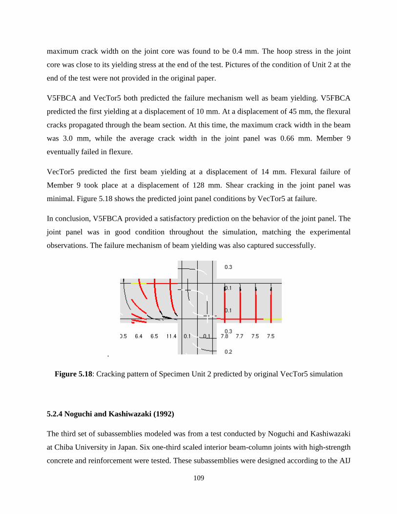
109
maximum crack width on the joint core was found to be 0.4 mm. The hoop stress in the joint
core was close to its yielding stress at the end of the test. Pictures of the condition of Unit 2 at the
end of the test were not provided in the original paper.
V5FBCA and VecTor5 both predicted the failure mechanism well as beam yielding. V5FBCA
predicted the first yielding at a displacement of 10 mm. At a displacement of 45 mm, the flexural
cracks propagated through the beam section. At this time, the maximum crack width in the beam
was 3.0 mm, while the average crack width in the joint panel was 0.66 mm. Member 9
eventually failed in flexure.
VecTor5 predicted the first beam yielding at a displacement of 14 mm. Flexural failure of
Member 9 took place at a displacement of 128 mm. Shear cracking in the joint panel was
minimal. Figure 5.18 shows the predicted joint panel conditions by VecTor5 at failure.
In conclusion, V5FBCA provided a satisfactory prediction on the behavior of the joint panel. The
joint panel was in good condition throughout the simulation, matching the experimental
observations. The failure mechanism of beam yielding was also captured successfully.
.
Figure 5.18: Cracking pattern of Specimen Unit 2 predicted by original VecTor5 simulation
5.2.4 Noguchi and Kashiwazaki (1992)
The third set of subassemblies modeled was from a test conducted by Noguchi and Kashiwazaki
at Chiba University in Japan. Six one-third scaled interior beam-column joints with high-strength
concrete and reinforcement were tested. These subassemblies were designed according to the AIJ

110
Guidelines (1988). One of the objectives was to study whether the provisions were applicable to
joints with high-strength materials and to establish a universal design method regardless of the
material strengths. Two of the six subassemblies, OKJ2 and OKJ6, were selected for verification.
Specimen OKJ2 was selected because the subassembly was tested under monotonic loading
conditions. Specimen OKJ6 was selected as a comparison companion because it had a lower
concrete strength than Specimen OKJ2. The other four specimens were excluded because they
presented only slightly different concrete strength and reinforcing details from the selected
specimens.
5.2.4.1 Test Specimens
Specimens OKJ2 and OKJ6 had identical overall dimensions, loading setup, and support
restrains, but the magnitudes of the column axial load were different. The subassemblies were
designed with different concrete strength and section properties. Figures 5.19 and 5.20 show the
test setup and sectional details, respectively. The dimensions of the beams were 300 by 200 mm,
and the dimensions of the columns were 300 by 300 mm. The longitudinal reinforcement in the
columns was designed to remain elastic. The joint panel was reinforced with three sets of
transverse tie reinforcement. Each set of reinforcement contained two ties. The material
properties of the concrete and the reinforcement are listed in Table 5.17. The subassemblies were
loaded by a displacement-controlled actuator. Constant compressive loads of 756 kN and 578 kN
were applied along the centerline of the column of Specimens OKJ2 and OKJ6, respectively.
Both ends of the beam were supported in the vertical direction. The bottom of the subassembly
was supported while the horizontal loading point was at the top of the column.
Table 5.17: Material properties of Specimens OKJ2 and OKJ6
Bar
Type
Reinforcement Properties
db
(mm)
Fy
(MPa)
Fu
(MPa)
Es
(MPa)
Esh*
(MPa)
εsh*
(x10-3
)
εu*
(x10-3
)
D13 13.0 718 767 186000 408 4.0 40.0
D6 6.0 955 1140 182000 5324 5.3 40.0
Spec.
Concrete Properties
f’c
(MPa)
f’t
(MPa)
Ec
(MPa)
ε’c
(x10-3
)
OKJ2 70.0 2.76 35100 2.96
OKJ6 53.5 2.41 36800 2.23
*: estimated

111
Figure 5.19: Test setup of Specimens OKJ2 and OKJ6 (Noguchi and Kashiwazaki, 1992)
Figure 5.20: Sectional details of Specimens OKJ2 and OKJ6: (a) beam section, (b) column
section, and (c) detailed joint reinforcement (Noguchi and Kashiwazaki, 1992)
5.4.3.2 Analytical Modeling
The subassemblies were modeled using the same structural model and boundary conditions, but
the loading and sectional properties were changed. Figure 5.21 shows the analytical model with
dimensions, loading, and support restraints. There were 33 nodes, 32 members, and 4 support
restraints in the model. Both Node 2 and Node 20 were restrained in the vertical direction. Node
22 was restrained in the horizontal and vertical directions. Column compressive loads of 756 kN
and 577.8 kN were applied at Node 33 of Specimens OKJ2 and OKJ6, respectively. In addition,
(a) (b) (c)

112
a positive horizontal displacement was applied at Node 33 in 161 load stages with an increment
of 1 mm starting from a zero displacement.
Figure 5.21: Analytical model showing dimensions, loading and support restraints of Specimens
OKJ2 and OKJ6
Six member types were created to build the model (see Figure 5.22). Member Types 1 and 2
were used to model the beam sections. Member Types 3 and 4 were used to model the column
sections. The interior joint was modeled by MT2 in the horizontal direction and MT4 in the
vertical direction. MT5 and MT6 were created by doubling the reinforcement ratios of MT2 and
MT4, respectively, to account for semi-rigid end offsets in the joint region. Each member was
divided into 20 to 22 concrete layers to perform the layered sectional analysis. Detailed general
and sectional material properties of Specimen OKJ2 are presented in Table 5.18, 5.19 and 5.20.
Specimen OKJ6 was modeled using a similar approach.
1330 150 150
585
150
1330
58
5
756 kN Displacement
(+1 mm)

113
Figure 5.22: Analytical model showing material types of Specimens OKJ2 and OKJ6
Table 5.18: General material specifications of Specimen OKJ2
MT
Concrete Properties Transverse Reinforcement Properties
f’c
(MPa)
f’t
(MPa)
Ec
(MPa)
ε’c
(x10-3
) Other
st
(mm)
dbt
(mm)
Fyt
(MPa)
Fut
(MPa)
Est
(MPa)
εsht
(x10-3
)
εut
(x10-3
) 1
70.0 2.76 35100 2.96 default
50 6.0 995 1140 182000 5 40
2 0 0 995 1140 182000 5 40
3 40 6 995 1140 182000 5 40
4 50 8.4 995 1140 182000 5 40
5 0 0 995 1140 182000 5 40
6 50 8.4 995 1140 182000 5 40
Table 5.19: Reinforced concrete material specifications of Specimen OKJ2
MT Dc
(mm)
Wc
(mm)
ρt
(%)
ρz
(%) Nx MT
Dc
(mm)
Wc
(mm)
ρt
(%)
ρz
(%) Nx
1
18.00
200
0.000 0.851 1
4
14.00
300
0.000 1.172 2
15.92 0.560 0.851 3 13.51 0.747 1.172 5
14.04 0.560 0.000 6 13.61 0.747 0.000 4
14.04 0.560 0.000 6 13.61 0.747 0.000 4
15.92 0.560 0.851 3 13.51 0.747 1.172 5
18.00 0.000 0.851 1 14.00 0.000 1.172 2
2
18.00
200
0.000 0.000 1
5
18.00
200
0.000 0.000 1
14.67 0.000 0.000 9 14.67 0.000 0.000 9
14.67 0.000 0.000 9 14.67 0.000 0.000 9
18.00 0.000 0.000 1 18.00 0.000 0.000 1
3
14.00
300
0.000 0.924 2
6
14.00
300
0.000 2.344 2
15.92 0.467 0.924 3 13.51 1.494 2.344 5
14.84 0.467 0.000 5 13.61 1.494 0.000 4
14.84 0.467 0.000 5 13.61 1.494 0.000 4
15.92 0.467 0.924 3 13.51 1.494 2.344 5
14.00 0.000 0.924 2 14.00 0.000 2.344 2
MT1
MT
3
MT1
MT
3
MT4 (MT6)
MT2 (MT5)

114
Table 5.20: Longitudinal reinforcement material specifications of Specimen OKJ2
MT N Ys
(mm)
As
(mm2)
Db
(mm)
Fy
(MPa)
Fu
(MPa)
Es
(MPa)
εsh
(x10-3
)
εu
(x10-3
)
1-2
1 30 660
13.0 718 767 186000 40 160 2 70 528
3 230 264
4 270 660
3-4
1 40 792
13.0 718 767 186000 40 160
2 84 264
3 128 264
4 172 264
5 216 264
6 260 792
5
1 30 1320
13.0 718 767 186000 40 160 2 70 1056
3 230 528
4 270 1320
6
1 40 1584
13.0 718 767 186000 40 160
2 84 528
3 128 528
4 172 528
5 216 528
6 260 1584
5.2.4.3 Comparison of the Analytical and Experimental Responses
Specimen OKJ2
Specimens OKJ2 and OKJ6 were analyzed with V5FBCA and VecTor5. A comparison of the
load-deflection responses at the column tip is given in Figure 5.23. Note that the positive
displacement was obtained from the backward loading condition in the experiment. Detailed
comparisons of the response parameters are reported in Table 5.21.
Table 5.21: Comparison of experimental and analytical results of Specimen OKJ2
Experiment V5FBCA VecTor5
Failure Mechanism BYJF BY BY
Peak Load (kN)
(Ratio = Analysis/Experiment)
237.0
265.6
(1.12)
274.7
(1.16)
Max. Panel Shear Stress (MPa)
(Ratio = Analysis/Experiment)
14.16
12.81
(0.90)
N/A
(N/A)
Load at First Beam Yielding (kN)
(Ratio = Analysis/Experiment)
237.0
245.9
(1.04)
241.4
(1.02)

115
Figure 5.23: Comparison of the load-displacement response of Specimen OKJ2
The subassembly exhibited the response mechanism of beam yielding followed by joint failure.
The joint shear cracks and splitting cracks along the column longitudinal bars were noticeable.
The beam bars yielded at the same time as the joint core reached its maximum shear strength.
The specimen attained a load of 230 kN at a displacement of 36 mm, and sustained this load up
to a displacement of 72 mm, where the subassembly lost its strength. At this time, the joint shear
distortion contributed to approximately 43% of the story drift. At a displacement of 36 mm, the
compressive strain in the concrete strut was measured to be approximately 4.5 x 10⁻³
. The
maximum shear strength of 14.2 MPa was reached at a displacement of 55 mm. The joint shear
distortion at the maximum shear strength was 26.0 x 10⁻³
. The maximum joint distortion was
40.0 x 10⁻³
at the failure of the structure. The bond of the beam longitudinal bars inside the joint
was in good condition. Figure 5.24 shows the cracking pattern of Specimen OKJ1, which had the
identical structural properties as Specimen OKJ2 with reversed cyclic loading applied to the
structure, at a displacement of 36 mm.
0
50
100
150
200
250
300
0 10 20 30 40 50 60 70 80
La
tera
l L
oa
d (
kN
)
Displacement (mm)
Experimental
V5FBCA
VecTor5

116
Figure 5.24: Cracking pattern of Specimen OKJ1 (Noguchi and Kashiwazaki, 1992)
The peak loads obtained from V5FBCA and VecTor5 were 12% and 16% higher than the
observed peak load, and they predicted the same failure mechanism due to beam yielding.
V5FBCA predicted a peak load of 265 kN at a displacement of 67 mm. The beam reinforcing
bars yielded on the left face of the joint panel at a displacement of 36 mm. With the increasing
applied displacement, the predicted average panel crack widths were 1.6 mm at a displacement
of 80 mm and 1.8 mm at a displacement of 100 mm. The joint core reached its maximum shear
stress of 12.8 MPa at a displacement of 158 mm, when the average crack width was 2.1 mm.
VecTor5 predicted a peak load of 274 kN at a displacement of 41 mm. The top longitudinal
reinforcement in Member 9 and the bottom longitudinal reinforcement in Member 12 reached the
yielding stress at a displacement of 19 mm. Flexural cracks with widths over 13 mm were found
in Members 9 and 12 at a displacement of 100 mm. The joint panel was calculated to be in good
condition throughout the simulation (see Figure 5.25a).
Overall, the analytical load-displacement response predicted by V5FBCA was better than
VecTor5 prediction in terms of the peak load, the maximum shear panel stress, and the load at
first beam yielding. However, the ductility of the subassembly was overestimated by 122%
compared to the observed ductility, resulting an inaccurate prediction of the failure mechanism
of the specimen.
The stresses obtained from the analysis were compared to those obtained from VecTor5 (see
Table 5.22). Bar stresses on the bottom and right faces were selected for the comparison. The
tensile stress predictions seemed to follow the VecTor5 results. However, the compressive
stresses on the right face predicted by V5FBCA were significantly different from the results
obtained from VecTor5.
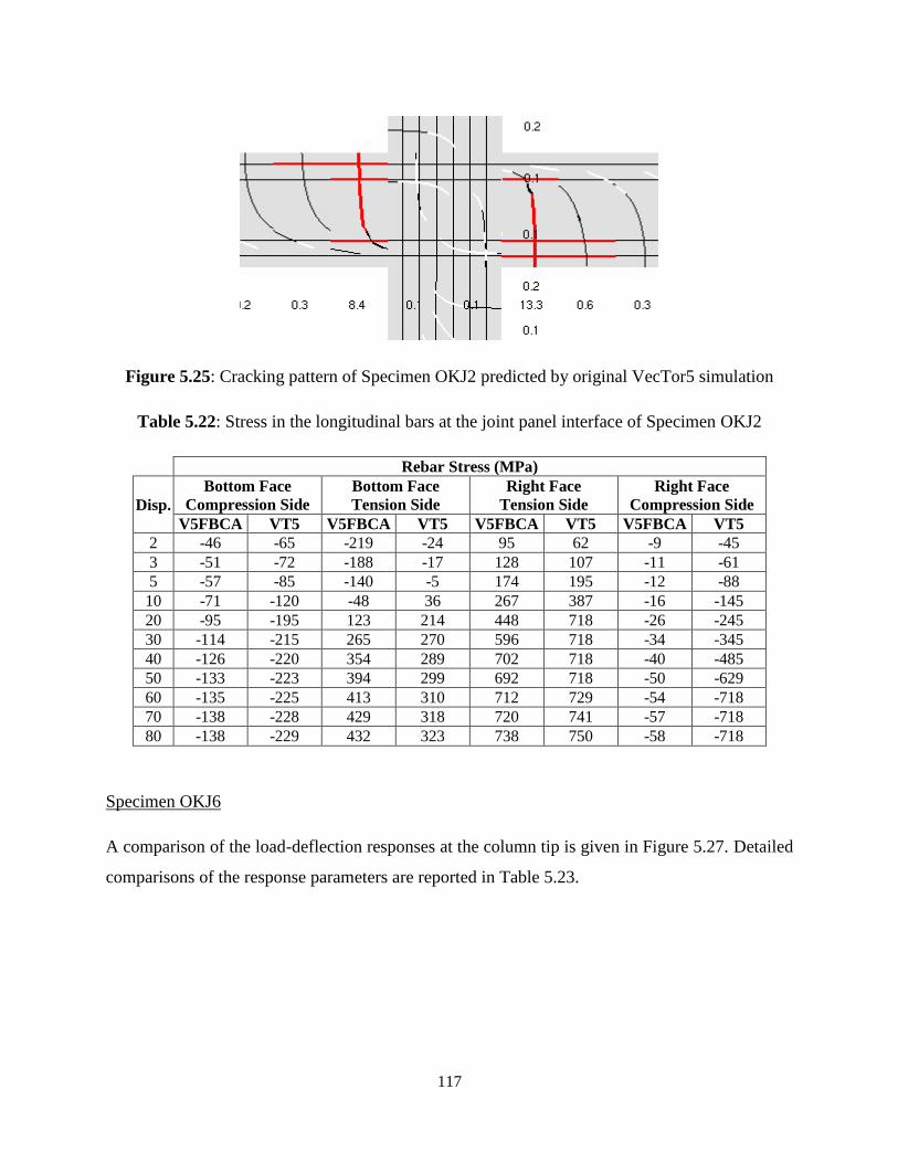
117
Figure 5.25: Cracking pattern of Specimen OKJ2 predicted by original VecTor5 simulation
Table 5.22: Stress in the longitudinal bars at the joint panel interface of Specimen OKJ2
Rebar Stress (MPa)
Disp.
Bottom Face
Compression Side
Bottom Face
Tension Side
Right Face
Tension Side
Right Face
Compression Side
V5FBCA VT5 V5FBCA VT5 V5FBCA VT5 V5FBCA VT5
2 -46 -65 -219 -24 95 62 -9 -45
3 -51 -72 -188 -17 128 107 -11 -61
5 -57 -85 -140 -5 174 195 -12 -88
10 -71 -120 -48 36 267 387 -16 -145
20 -95 -195 123 214 448 718 -26 -245
30 -114 -215 265 270 596 718 -34 -345
40 -126 -220 354 289 702 718 -40 -485
50 -133 -223 394 299 692 718 -50 -629
60 -135 -225 413 310 712 729 -54 -718
70 -138 -228 429 318 720 741 -57 -718
80 -138 -229 432 323 738 750 -58 -718
Specimen OKJ6
A comparison of the load-deflection responses at the column tip is given in Figure 5.27. Detailed
comparisons of the response parameters are reported in Table 5.23.
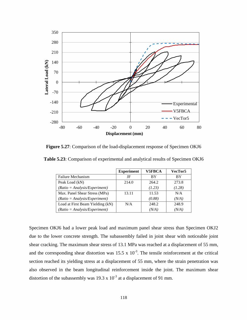
118
Figure 5.27: Comparison of the load-displacement response of Specimen OKJ6
Table 5.23: Comparison of experimental and analytical results of Specimen OKJ6
Experiment V5FBCA VecTor5
Failure Mechanism JF BY BY
Peak Load (kN)
(Ratio = Analysis/Experiment)
214.0
264.2
(1.23)
273.8
(1.28)
Max. Panel Shear Stress (MPa)
(Ratio = Analysis/Experiment)
13.11
11.53
(0.88)
N/A
(N/A)
Load at First Beam Yielding (kN)
(Ratio = Analysis/Experiment)
N/A
248.2
(N/A)
248.9
(N/A)
Specimen OKJ6 had a lower peak load and maximum panel shear stress than Specimen OKJ2
due to the lower concrete strength. The subassembly failed in joint shear with noticeable joint
shear cracking. The maximum shear stress of 13.1 MPa was reached at a displacement of 55 mm,
and the corresponding shear distortion was 15.5 x 10⁻³
. The tensile reinforcement at the critical
section reached its yielding stress at a displacement of 55 mm, where the strain penetration was
also observed in the beam longitudinal reinforcement inside the joint. The maximum shear
distortion of the subassembly was 19.3 x 10⁻³
at a displacement of 91 mm.
-280
-210
-140
-70
0
70
140
210
280
350
-80 -60 -40 -20 0 20 40 60 80
Late
ral
Load
(k
N)
Displacement (mm)
Experimental
V5FBCA
VecTor5
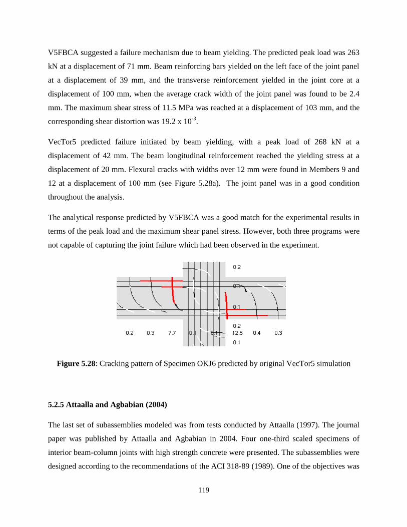
119
V5FBCA suggested a failure mechanism due to beam yielding. The predicted peak load was 263
kN at a displacement of 71 mm. Beam reinforcing bars yielded on the left face of the joint panel
at a displacement of 39 mm, and the transverse reinforcement yielded in the joint core at a
displacement of 100 mm, when the average crack width of the joint panel was found to be 2.4
mm. The maximum shear stress of 11.5 MPa was reached at a displacement of 103 mm, and the
corresponding shear distortion was 19.2 x 10⁻³
.
VecTor5 predicted failure initiated by beam yielding, with a peak load of 268 kN at a
displacement of 42 mm. The beam longitudinal reinforcement reached the yielding stress at a
displacement of 20 mm. Flexural cracks with widths over 12 mm were found in Members 9 and
12 at a displacement of 100 mm (see Figure 5.28a). The joint panel was in a good condition
throughout the analysis.
The analytical response predicted by V5FBCA was a good match for the experimental results in
terms of the peak load and the maximum shear panel stress. However, both three programs were
not capable of capturing the joint failure which had been observed in the experiment.
Figure 5.28: Cracking pattern of Specimen OKJ6 predicted by original VecTor5 simulation
5.2.5 Attaalla and Agbabian (2004)
The last set of subassemblies modeled was from tests conducted by Attaalla (1997). The journal
paper was published by Attaalla and Agbabian in 2004. Four one-third scaled specimens of
interior beam-column joints with high strength concrete were presented. The subassemblies were
designed according to the recommendations of the ACI 318-89 (1989). One of the objectives was

120
to understand whether the definition of the joint shear strength as a function of the square root of
the concrete compressive strength was applicable to high strength concrete. Three joint
subassemblies, SHC1, SHC2 and SOC3 were selected for verification. Specimen SHC3 was
excluded because the joint core was reinforced with steel fibers.
5.2.5.1 Test Specimens
The subassemblies had identical overall dimensions, loading setup, and support restraints, but the
joint reinforcement and concrete properties were different. Figures 5.29 and 5.30 show the test
setup and the sectional details, respectively. The beam was 203 by 127 mm, and the column was
178 by 127 mm. The subassemblies were designed to exhibit joint shear damage mechanisms
under earthquake loading. The joint panel of Specimen SHC1 was reinforced by one transverse
tie, whereas the joint panel of Specimens SHC2 and SOC3 were reinforced by two transverse ties.
The material properties of the high strength concrete and the reinforcement are listed in Table
5.24. The subassemblies were loaded in a displacement-controlled mode. A constant
compressive load of 58 kN was applied along the centerline of the column. The subassemblies
were supported by a hinged support at the right end of the beam and two roller supports at the
top and bottom of the column. The displacement was applied in the vertical direction at the left
end of the beam.
Figure 5.29: Test setup of Specimens SHC1, SHC2 and SOC3 (Attaalla and Agbabian, 2004)

121
Table 5.24: Material properties of Specimens SHC1, SHC2 and SOC3
Figure 5.30: Sectional details of Specimens SHC1, SHC2 and SOC3: (a) beam section, (b)
column section (Attaalla and Agbabian, 2004), and (c) detailed joint reinforcement (Attaalla,
1997)
5.2.5.2 Analytical Modeling
The two subassemblies were modeled using the same structural model, applied loading, and
boundary conditions, but with differing concrete properties. Figure 5.31 shows the analytical
model with dimensions, loading, and support restraints. There were 33 nodes, 32 members, and 4
support restraints in the model. Node 23 was restrained in the horizontal and vertical directions
for a hinge support, and Nodes 24 and 33 were restrained in the horizontal direction for roller
supports. A column compressive load of 58 kN was modeled by applying compressive nodal
forces at Nodes 24 and 33. In addition, a negative vertical displacement was applied at the left
end of the beam in 61 load stages with an increment of 2 mm starting from a zero displacement.
Bar
Type
Reinforcement Properties
db
(mm)
Fy
(MPa)
Fu
(MPa)
Es
(MPa)
Esh*
(MPa)
εsh*
(x10-3
)
εu*
(x10-3
)
#4 12.7 414 620 200000 2289 10.0 100.0
#3 9.53 414 620 200000 2289 10.0 100.0
#2 6.35 552 650 200000 1089 10.0 100.0
Spec.
Concrete Properties
f’c
(MPa)
f’t*
(MPa)
Ec*
(MPa)
ε’c
(x10-3
)
SHC1 56.6 2.48 30165 3.75
SHC2 59.6 2.55 29790 4.00
SOC3 47.2 2.27 31453 3.50
*: estimated
(a) (b) (c)
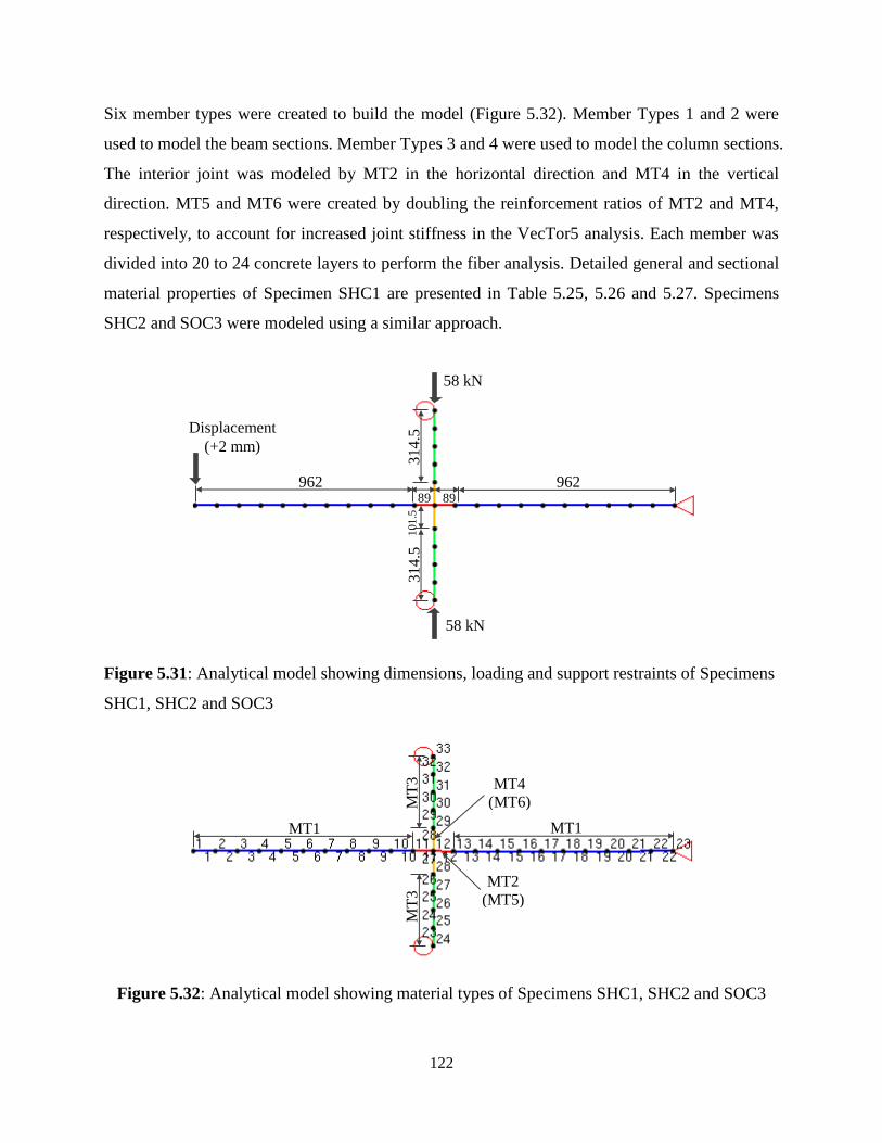
122
Six member types were created to build the model (Figure 5.32). Member Types 1 and 2 were
used to model the beam sections. Member Types 3 and 4 were used to model the column sections.
The interior joint was modeled by MT2 in the horizontal direction and MT4 in the vertical
direction. MT5 and MT6 were created by doubling the reinforcement ratios of MT2 and MT4,
respectively, to account for increased joint stiffness in the VecTor5 analysis. Each member was
divided into 20 to 24 concrete layers to perform the fiber analysis. Detailed general and sectional
material properties of Specimen SHC1 are presented in Table 5.25, 5.26 and 5.27. Specimens
SHC2 and SOC3 were modeled using a similar approach.
Figure 5.31: Analytical model showing dimensions, loading and support restraints of Specimens
SHC1, SHC2 and SOC3
Figure 5.32: Analytical model showing material types of Specimens SHC1, SHC2 and SOC3
962 89 89
314.5
1
01
.5
962
314.5
58 kN
58 kN
MT1
MT
3
MT1
MT
3
MT4 (MT6)
MT2 (MT5)
Displacement
(+2 mm)

123
Table 5.25: General material specifications of Specimen SHC1
MT
Concrete Properties Transverse Reinforcement Properties
f’c
(MPa)
f’t
(MPa)
Ec
(MPa)
ε’c
(x10-3
) Other
st
(mm)
dbt
(mm)
Fyt
(MPa)
Fut
(MPa)
Est
(MPa)
εsht
(x10-3
)
εut
(x10-3
) 1
56.6 2.48 30165 3.75 default
76 6.4 552 650 200000 10 100
2 0 0 -- -- -- -- -- 3 51 6.4 552 650 200000 10 100
4 101.5 6.4 552 650 200000 10 100
5 0 0 -- -- -- -- -- 6 101.5 6.4 552 650 200000 10 100
Table 5.26: Reinforced concrete material specifications of Specimen SHC1
MT Dc
(mm)
Wc
(mm)
ρt
(%)
ρz
(%) Nx MT
Dc
(mm)
Wc
(mm)
ρt
(%)
ρz
(%) Nx
1
10.0
127
0.000 0.592 2
4
10.0
127
0.000 0.444 2
8.51 0.663 0.592 6 8.51 0.496 0.444 6
7.61 0.663 0.000 4 8.97 0.496 0.000 2
7.61 0.663 0.000 4 8.97 0.496 0.000 2
8.51 0.663 0.592 6 8.51 0.496 0.444 6
10.0 0.000 0.592 2 10.0 0.000 0.444 2
2
10.0
127
0.000 0.000 2
5
10.0
127
0.000 0.000 2
10.19 0.000 0.000 8 10.19 0.000 0.000 8
10.19 0.000 0.000 8 10.19 0.000 0.000 8
10.0 0.000 0.000 2 10.0 0.000 0.000 2
3
10.0
127
0.000 0.883 2
6
10.0
127
0.000 0.888 2
8.51 0.988 0.883 6 8.51 0.992 0.888 6
8.97 0.988 0.000 2 8.97 0.992 0.000 2
8.97 0.988 0.000 2 8.97 0.992 0.000 2
8.51 0.988 0.883 6 8.51 0.992 0.888 6
10.0 0.000 0.883 2 10.0 0.000 0.888 2
Table 5.27: Longitudinal reinforcement material specifications of Specimen SHC1
MT N Ys
(mm)
As
(mm2)
Db
(mm)
Fy
(MPa)
Fu
(MPa)
Es
(MPa)
εsh
(x10-3
)
εu
(x10-3
)
1-2 1 32 213
9.5 414 620 200000 10 100 2 171 213
3-4 1 32 258
12.8 414 620 200000 10 100 2 171 258
5 1 33 426
9.5 414 620 200000 10 100 2 145 426
6 1 33 516
12.8 414 620 200000 10 100 2 145 516

124
5.2.5.3 Comparison of the Analytical and Experimental Responses
Specimen SHC1
The three subassemblies were analyzed with V5FBCA and VecTor5. A comparison of the
vertical load-deflection responses at Node 1 is shown in Figure 5.33. Detailed comparisons of the
response parameters are reported in Table 5.28.
Figure 5.33: Comparison of the load-displacement response of Specimen SHC1
Table 5.28: Comparison of experimental and analytical results of Specimen SHC1
Experiment V5FBCA VecTor5
Failure Mechanism BYJF BYJF BY
Peak Load (kN)
(Ratio = Analysis/Experiment)
16.02
16.38
(1.02)
21.47
(1.34)
Max. Panel Shear Stress (MPa)
(Ratio = Analysis/Experiment)
6.88
5.21
(0.76)
N/A
(N/A)
Load at First Beam Yielding (kN)
(Ratio = Analysis/Experiment)
11.90
15.91
(1.34)
15.42
(1.30)
-20
-15
-10
-5
0
5
10
15
20
25
-120 -90 -60 -30 0 30 60 90 120
Load
(k
N)
Displacement (mm)
Experiment
V5FBCA
VecTor5

125
The failure of the subassembly was mainly due to the shear mechanism in the joint core, but
damage in beams close to the column faces was noticeable. Figure 5.34a shows the cracking
pattern of Specimen SHC1 at the end of the test. The peak load was 16.02 kN at a displacement
of 100 mm. The longitudinal reinforcement of the beams yielded at the joint interface at a
displacement of 28 mm. The maximum shear stress of the joint panel was 6.88 MPa with the
corresponding maximum shear distortion of 12.7 x 10⁻³
.
V5FBCA predicted the failure mechanism as beam yielding followed by joint failure, matching
well with the experimental observations. The original VecTor5, on the other hand, predicted the
failure mechanism due to beam yielding. V5FBCA predicted a peak load of 16.4 kN at a
displacement of 54 mm. The longitudinal reinforcement of the beam yielded at both sides of the
column interface at a displacement of 36 mm. The column steel did not yield throughout the
simulation. The maximum shear stress of 5.2 MPa was reached at a displacement of 50 mm with
the corresponding shear strain of 9.0 x 10⁻³
. The average crack width was 1.1 mm. The joint
transverse reinforcement yielded at a displacement of 54 mm, at which point the structure started
losing its strength and the load gradually declined.
VecTor5 predicted a load of 21.5 kN at a displacement of 100 mm. The longitudinal
reinforcement of the beam yielded at a displacement of 18 mm. The column steel yielded at a
displacement of 42 mm. Flexural cracking in the beams close to the joint panel was noticeable at
a displacement of 100 mm (see Figure 5.34b).
Overall, the analytical response predicted by V5FBCA was a good match for the experimental
results in terms of the peak load and the stiffness of the subassembly. V5FBCA successfully
captured the failure mechanism as beam yielding followed by joint failure.
The stresses obtained from the analysis were compared to those obtained from VecTor5 and (see
Table 5.29). The stresses on the top and left faces of the joint panel were selected for the
comparison because cracking was expected to form near these interfaces. The tensile stresses in
the longitudinal steel predicted by V5FBCA were slightly lower than the values from VecTor5.
On the other hand, the compressive stresses in the beam bars predicted by V5FBCA showed
some disagreement with the values from VecTor5.

126
Figure 5.34: Cracking pattern of Specimen SHC1: (a) observed (Attaalla and Agbabian, 2004)
and (b) original VecTor5 simulation
Table 5.29: Stress in the longitudinal bars at the joint panel interface of Specimen SHC1
Rebar Stress (MPa)
Disp.
Top Face
Tension Side
Top Face
Compression Side
Left Face
Compression Side
Left Face
Tension Side
V5FBCA VT5 V5FBCA VT5 V5FBCA VT5 V5FBCA VT5
2 -23 -3 -69 -39 -6 -21 8 22
3 -28 12 -43 -54 -10 -40 14 68
5 17 65 -37 -80 -3 -63 132 166
10 148 238 -57 -127 -6 -102 252 414
15 243 304 -72 -142 -8 12 343 435
20 300 339 -80 -159 -8 60 403 470
25 326 414 -84 -156 -6 84 437 490
30 286 414 -78 -122 -2 110 428 507
Specimen SHC2
A comparison of the vertical load-deflection responses at Node 1 is presented in Figure 5.35.
Detailed comparisons of the response parameters are reported in Table 5.30.
Table 5.30: Comparison of experimental and analytical results of Specimen SHC2
Experiment V5FBCA VecTor5
Failure Mechanism BYJF BYJF BY
Peak Load (kN)
(Ratio = Analysis/Experiment)
16.73
18.36
(1.10)
21.55
(1.29)
Max. Panel Shear Stress (MPa)
(Ratio = Analysis/Experiment)
7.24
5.80
(0.80)
N/A
(N/A)
Load at First Beam Yielding (kN)
(Ratio = Analysis/Experiment)
12.20
15.92
(1.30)
16.08
(1.32)
(a) (b)

127
Figure 5.35: Comparison of the load-displacement response of Specimen SHC2
Specimen SHC2 had two transverse ties in the joint core as opposed of one transverse tie in
Specimen SHC1. It was expected that the addition of the transverse reinforcement would delay
the formation of joint shear cracks, but two major diagonal cracks formed early at a displacement
of 28 mm, which was the same as the case for Specimen SHC1. The failure of the subassembly
was mainly due to the shear mechanism in the joint core, but damage in the beams close to the
column faces was noticeable. Figure 5.36a shows the cracking pattern of Specimen SHC2 at the
end of the test. The peak load was 16.7 kN at a displacement of 100 mm. The longitudinal
reinforcement of the beams yielded at the joint interface at a displacement of 28 mm. The
maximum shear stress of the joint panel was 7.24 MPa with the corresponding maximum shear
distortion of 8.7 x 10⁻³
. The additional transverse reinforcement increased the joint shear strength
by only 5%, but it significantly reduced the joint shear deformation by 45%.
V5FBCA predicted the failure mechanism as beam yielding followed by joint failure, matching
well with the experimental observations. The original VecTor5, on the other hand, predicted the
failure mechanism due to beam yielding. V5FBCA predicted a peak load of 18.4 kN at a
displacement of 86 mm. The longitudinal reinforcement of the beam yielded at the left column
-20
-15
-10
-5
0
5
10
15
20
25
-120 -90 -60 -30 0 30 60 90 120
Load
(k
N)
Displacement (mm)
Experiment
V5FBCA
VecTor5

128
interface at a displacement of 38 mm. The transverse reinforcement yielded at a displacement of
66 mm, when the structure started losing its strength and the load slowly declined. The
maximum shear stress of 5.8 MPa was reached at a displacement of 82 mm with the
corresponding shear strain of 12.2 x 10⁻³
. The average crack width was 1.4 mm at this time.
VecTor5 predicted a load capacity of 21.6 kN at a displacement of 100 mm. The longitudinal
reinforcement of the beam yielded at a displacement of 20 mm. The column steel yielded at a
displacement of 44 mm. Flexural cracking in the beams close to the joint panel was noticeable at
a displacement of 100 mm. The joint was in good condition without noticeable shear cracking
(see Figure 5.36b).
In conclusion, the analytical response predicted by V5FBCA was a good match for the
experimental results in terms of the peak load and the stiffness of the subassembly. V5FBCA
successfully captured the failure mechanism as beam yielding followed by joint failure. The
response of the joint shear panel was predicted reasonably well.
Figure 5.36: Cracking pattern of Specimen SHC2: (a) observed (Attaalla and Agbabian, 2004)
and (b) original VecTor5 simulation
Specimen SOC3
A comparison of the vertical load-deflection responses at Node 1 is given in Figure 5.37.
Detailed comparisons of the response parameters are reported in Table 5.31.
(a) (b)
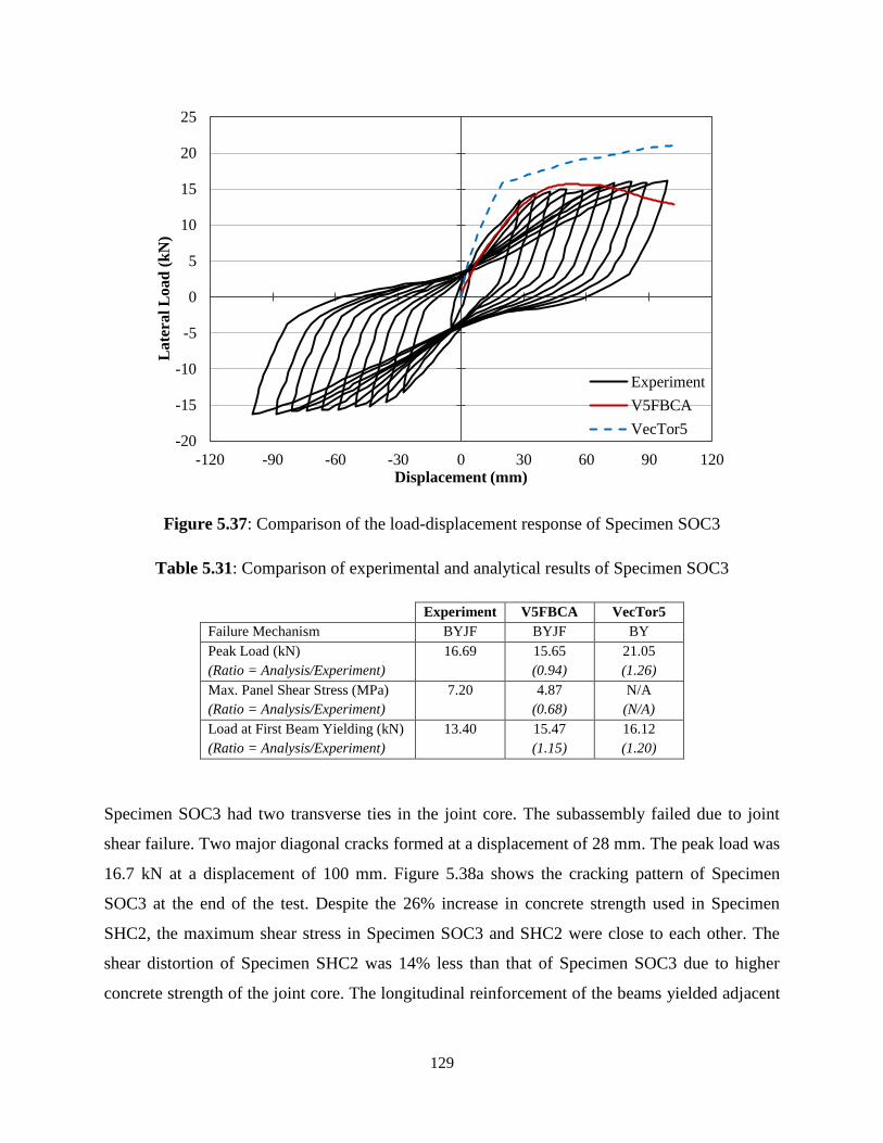
129
Figure 5.37: Comparison of the load-displacement response of Specimen SOC3
Table 5.31: Comparison of experimental and analytical results of Specimen SOC3
Experiment V5FBCA VecTor5
Failure Mechanism BYJF BYJF BY
Peak Load (kN)
(Ratio = Analysis/Experiment)
16.69
15.65
(0.94)
21.05
(1.26)
Max. Panel Shear Stress (MPa)
(Ratio = Analysis/Experiment)
7.20
4.87
(0.68)
N/A
(N/A)
Load at First Beam Yielding (kN)
(Ratio = Analysis/Experiment)
13.40
15.47
(1.15)
16.12
(1.20)
Specimen SOC3 had two transverse ties in the joint core. The subassembly failed due to joint
shear failure. Two major diagonal cracks formed at a displacement of 28 mm. The peak load was
16.7 kN at a displacement of 100 mm. Figure 5.38a shows the cracking pattern of Specimen
SOC3 at the end of the test. Despite the 26% increase in concrete strength used in Specimen
SHC2, the maximum shear stress in Specimen SOC3 and SHC2 were close to each other. The
shear distortion of Specimen SHC2 was 14% less than that of Specimen SOC3 due to higher
concrete strength of the joint core. The longitudinal reinforcement of the beams yielded adjacent
-20
-15
-10
-5
0
5
10
15
20
25
-120 -90 -60 -30 0 30 60 90 120
La
tera
l L
oa
d (
kN
)
Displacement (mm)
Experiment
V5FBCA
VecTor5

130
to the joint interface at a displacement of approximately 28 mm. The maximum shear stress of
the joint panel was 7.2 MPa with the corresponding maximum shear distortion of 10.2 x 10⁻³
.
V5FBCA predicted the failure mechanism as beam yielding followed by joint failure, matching
well with the experimental observations. Once again, the original VecTor5 predicted the failure
mechanism as beam yielding. V5FBCA predicted a peak load of 15.7 kN at a displacement of
100 mm. The longitudinal reinforcement of the beam yielded at the left column interface at a
displacement of 43 mm. The transverse reinforcement yielded at a displacement of 45 mm,
where the structure started losing its strength and the load slowly started to decline. The
maximum shear stress of 4.9 MPa was also reached at a displacement of 54 mm with the
corresponding shear strain of 11.9 x 10⁻³
. At this time, the average crack width was 1.4 mm.
VecTor5 predicted a load of 21.1 kN at a displacement of 100 mm. The longitudinal
reinforcement of the beam yielded at a displacement of 22 mm. The column steel yielded at a
displacement of 44 mm. Flexural cracking in beams close to the joint panel was noticeable at a
displacement of 100 mm. The joint was in good condition without noticeable shear cracking (see
Figure 5.38b).
Overall, the analytical response predicted by V5FBCA was a good match for the experimental
results in terms of the peak load and the stiffness of the subassembly. V5FBCA successfully
captured the failure mechanism as beam yielding followed by joint failure.
A comparison of the envelopes of the beam shear force versus the panel shear strain is given in
Figure 5.39. Attaalla and Agbabian concluded that increasing the amount of joint ties in
Specimens SHC2 and SOC3 did not affect the shear stiffness of the joint. The change in slope of
the curve was due to the formation of the main diagonal cracks at a displacement of 28 mm. The
analytical response was plotted up to the shear strain at the maximum panel shear stress. The
analytical responses showed good correlation with the experimental results in terms of the
maximum load. However, the stiffness of the joint panel prior to the formation of the main
diagonal cracks did not match well with the observed results. The analysis also predicted greater
maximum panel shear strain of Specimens SHC2 and SOC3 than that of Specimen SHC1 due to
the increasing amount of transverse reinforcement in the joint core.

131
Figure 5.38: Cracking pattern of Specimen SOC3: (a) observed (Attaalla and Agbabian, 2004)
and (b) VecTor5 simulation
(a) (b) (c)
Figure 5.39: Envelopes of the load versus the panel shear strain relationships for: (a) Specimen
SHC1, (b) Specimen SHC2, and (c) Specimen SOC3
0
3
6
9
12
15
18
21
0 3 6 9 12
Lo
ad
(k
N)
Panel Shear Strain (kN)
Experiment
V5FBCA
0
3
6
9
12
15
18
21
0 3 6 9 12
Lo
ad
(k
N)
Panel Shear Strain (kN)
Experiment
V5FBCA
0
3
6
9
12
15
18
21
0 3 6 9 12
Lo
ad
(k
N)
Panel Shear Strain (kN)
Experiment
V5FBCA
(a) (b)

132
5.3 Parametric Study of Beam-Column Joint Subassemblies
Parametric studies were carried out to investigate the impact of four parameters on the load-
displacement response of the subassemblies. The parameters include: loading type, confinement,
compression softening, and bond stress. The impact of the loading type was studied in order to
understand whether the backbone curve of the reversed cyclic response was a good
representation of the monotonic response. To assess the impact of the loading type on the load-
displacement response, a comparison involving the response of Specimen OKJ2 tested under the
monotonic and reversed cyclic loading conditions is presented in Figure 5.40. In this example,
the stiffness of the subassembly prior to 30 mm story drift and the peak load for both loading
conditions were similar. However, the monotonic response was able to sustain the peak load, but
the reversed cyclic response showed the loss of stiffness. In addition, the analytical responses
under monotonic and reversed cyclic loading conditions were compared. Figure 5.41 shows a
comparison of the VecTor5 analytical load-displacement responses of Specimen A1. In this
example, the monotonic response curve was capable of capturing the initial and post-yielding
stiffness of the reversed cyclic response. The peak loads and the load at first beam yielding
simulated under the monotonic and reversed cyclic loading conditions were also comparable. In
conclusion, the backbone curve of the reversed cyclic response was a good representation of the
monotonic response in terms of the peak load and the initial stiffness of the structure. However,
the loss of stiffness due to the hysteretic response may not be captured by the monotonic
response.
Figure 5.40: Story shear force versus story drift relationships of Specimen OKJ2 (Noguchi and
Kashiwazaki, 1992) subjected to: (a) monotonic and (b) reversed cyclic loading conditions
(a) (b)

133
Figure 5.41: Comparison of the VecTor5 load-displacement responses of Specimen A1
The second parameter was the impact of the confinement effectiveness coefficient, which
considers the confinement in the column section as well as the confinement contributed by the
transverse reinforcement in the joint core. The formulation details were provided in Section 4.3.3.
The value of 1.0 represents a fully confined joint core, whereas the value of 0 represents joints
with no or ineffective transverse reinforcement. The subassemblies were tested under these two
conditions and the load-displacement responses were compared to the original analytical
response (see Figure 5.42). It was observed that confinement from the transverse reinforcement
delayed concrete crushing of the joint core, providing greater strength for subassemblies that
exhibited significant joint damage.
-200
-150
-100
-50
0
50
100
150
200
-80.0 -60.0 -40.0 -20.0 0.0 20.0 40.0 60.0 80.0
Lo
ad
(k
N)
Displacement (mm)
VecTor5 (Monotonic)
VecTor5 (Reversed Cyclic)

134
Figure 5.42: Comparison of the load-displacement responses with different confinement
effectiveness coefficients
0
30
60
90
120
150
180
0 20 40 60 80
Lo
ad
(k
N)
Displacement (mm)
SK-A1
k=0.786
VT5
k=1
k=0.001
0
30
60
90
120
150
180
0 20 40 60 80L
oa
d (
kN
)
Displacement (mm)
SK-A2
k=0.702
VT5
k=1
k=0.001
0
5
10
15
20
25
0 30 60 90 120
Lo
ad
(k
N)
Displacement (mm)
AA-SHC1
k=0.102VT5k=1k=0.001
0
30
60
90
120
0 25 50 75 100 125
Lo
ad
(k
N)
Displacement (mm)
PD-U1
k=0.56
VT5
k=1
k=0.001
0
30
60
90
120
150
0 30 60 90 120 150
Lo
ad
(k
N)
Displacement (mm)
PD-U2
k=0.57VT5k=1k=0.001
0
5
10
15
20
25
0 30 60 90 120
Lo
ad
(k
N)
Displacement (mm)
AA-SHC2
k=0.189VT5k=1k=0.001
0
50
100
150
200
250
300
0 20 40 60 80 100
Lo
ad
(k
N)
Displacement (mm)
NK-OKJ2
k=0.786VT5k=1k=0.001
0
50
100
150
200
250
300
0 20 40 60 80 100
Lo
ad
(k
N)
Displacement (mm)
NK-OKJ6
k=0.786VT5k=1k=0.001
0
5
10
15
20
25
0 30 60 90 120
Lo
ad
(k
N)
Displacement (mm)
AA-SOC3
k=0.189VT5k=1k=0.001

135
The next parameter investigated was the impact of the reduction factor due to the compression
softening effect. The formulation details were provided in Section 3.4. The reduction factor of
1.0 was selected to represent no strength reduction due to joint cracking. In was anticipated that
the obtained load-displacement response would be close to the response from the original
VecTor5 with semi-rigid end offsets. This was verified by a comparison of the responses as
shown in Figure 5.43. The investigation concluded that the response predicted by V5FBCA was
similar to the original VecTor5 prediction with the consideration of the joint response.
0
30
60
90
120
150
180
0 20 40 60 80
Lo
ad
(k
N)
Displacement (mm)
SK-A1
V5FBCA
VT5
No Soft.0
30
60
90
120
150
180
0 20 40 60 80
Lo
ad
(k
N)
Displacement (mm)
SK-A2
V5FBCA
VT5
No Soft.0
5
10
15
20
25
0 30 60 90 120L
oa
d (
kN
)
Displacement (mm)
AA-SHC1
V5FBCAVT5No Soft.
0
30
60
90
120
0 25 50 75 100 125
Lo
ad
(k
N)
Displacement (mm)
PD-U1
V5FBCA
VT5
No Soft.0
30
60
90
120
150
0 30 60 90 120 150
Lo
ad
(k
N)
Displacement (mm)
PD-U2
V5FBCAVT5No Soft.
0
5
10
15
20
25
0 30 60 90 120
Lo
ad
(k
N)
Displacement (mm)
AA-SHC2
V5FBCAVT5No Soft.

136
Figure 5.43: Comparison of the load-displacement responses without the compression softening
effect
The last parameter examined was the bond stress. Uniform bond stresses were assumed along the
longitudinal bars in the joint core depending on the rebar conditions as presented in Table 3.1. In
order to assess the impact of the assumed bond stress on the load-displacement response, bi-
uniform bond stresses proposed by Sezen and Moehle (2003) were employed and tested.
Formulation details of the bond model were presented in Section 2.3.3. A comparison of the
responses shown in Figure 5.44 concluded that the assumption of the bond stresses did not have
a significant impact on the global load-displacement response for the subassemblies. This may be
explained by the observation that the subassemblies did not exhibit major bond damage or failure
during the tests.
0
50
100
150
200
250
300
0 20 40 60 80 100
Lo
ad
(k
N)
Displacement (mm)
NK-OKJ2
V5FBCAVT5No Soft.
0
50
100
150
200
250
300
0 20 40 60 80 100L
oa
d (
kN
)
Displacement (mm)
NK-OKJ6
V5FBCAVT5No Soft.
0
5
10
15
20
25
0 30 60 90 120
Lo
ad
(k
N)
Displacement (mm)
AA-SOC3
V5FBCAVT5No Soft.
0
30
60
90
120
150
180
0 20 40 60 80
Lo
ad
(k
N)
Displacement (mm)
SK-A1
V5FBCA
VT5
Sezen (2003)0
30
60
90
120
150
180
0 20 40 60 80
Lo
ad
(k
N)
Displacement (mm)
SK-A2
V5FBCA
VT5
Sezen (2003)0
5
10
15
20
25
0 30 60 90 120
Lo
ad
(k
N)
Displacement (mm)
AA-SHC1
V5FBCAVT5Sezen (2003)
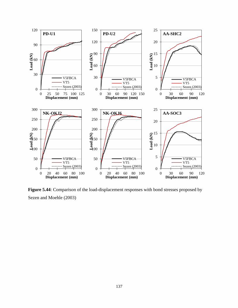
137
Figure 5.44: Comparison of the load-displacement responses with bond stresses proposed by
Sezen and Moehle (2003)
0
30
60
90
120
0 25 50 75 100 125
Lo
ad
(k
N)
Displacement (mm)
PD-U1
V5FBCA
VT5
Sezen (2003)0
30
60
90
120
150
0 30 60 90 120 150L
oa
d (
kN
)
Displacement (mm)
PD-U2
V5FBCAVT5Sezen (2003)
0
5
10
15
20
25
0 30 60 90 120
Lo
ad
(k
N)
Displacement (mm)
AA-SHC2
V5FBCAVT5Sezen (2003)
0
50
100
150
200
250
300
0 20 40 60 80 100
Lo
ad
(k
N)
Displacement (mm)
NK-OKJ2
V5FBCAVT5Sezen (2003)
0
50
100
150
200
250
300
0 20 40 60 80 100
Lo
ad
(k
N)
Displacement (mm)
NK-OKJ6
V5FBCAVT5Sezen (2003)
0
5
10
15
20
25
0 30 60 90 120
Lo
ad
(k
N)
Displacement (mm)
AA-SOC3
V5FBCAVT5Sezen (2003)

138
5.4 Frame Structures
5.4.1 Summary
In order to assess the performance of VecTor5 with the new joint element, three large-scale
frame structures with different joint reinforcement ratios were selected for evaluation and
verification. The frame structures were analyzed with V5FBCA and the original VecTor5.
The inputs used for the analyses with V5FBCA and VecTor5 were almost identical. The only
difference was that the semi-rigid end offsets were not used for interior joints in the analysis with
V5FBCA. The external and knee joints, on the other hand, were modeled with the semi-rigid end
offsets in both analyses. Once again, the default or typical material behavior models to assess the
capabilities without using special program modifications.
The analytical load-deflection responses from V5FBCA and VecTor5 were compared with the
experimental responses. The failure mechanisms and the cracking patterns of the frame
structures were also compared in the study. The analytical responses, failure mechanism, and
response from V5FBCA showed good correlation with the experimental results.
5.4.2 Xue et al. Frame (2011)
An experimental program was conducted to investigate the seismic performance of high-
performance concrete frames under low reversed cyclic loading (Xue et al., 2011). The
experiment involved testing two specimens of a one-fifth scale, two-story, two-bay high-
performance concrete frames under constant vertical loads and applied reversed cyclic loads. The
frame specimens were detailed in conformity with the requirements of ACI 318-08 (2008). One
of the frames, HPCF-1, was selected for evaluation and verification. The other specimen was
excluded because it involved prestressing.
The test frame was constructed with a center-to-center span of 2700 mm, a story height of 1000
mm and an overall height of 2610 mm (see Figure 5.45). All beams were 220 mm deep and 150
mm wide, and all columns were 200 mm deep and 200 mm wide. The frame was built integral
with a heavily reinforced base which was 300 mm deep and 300 mm wide. The base was bolted
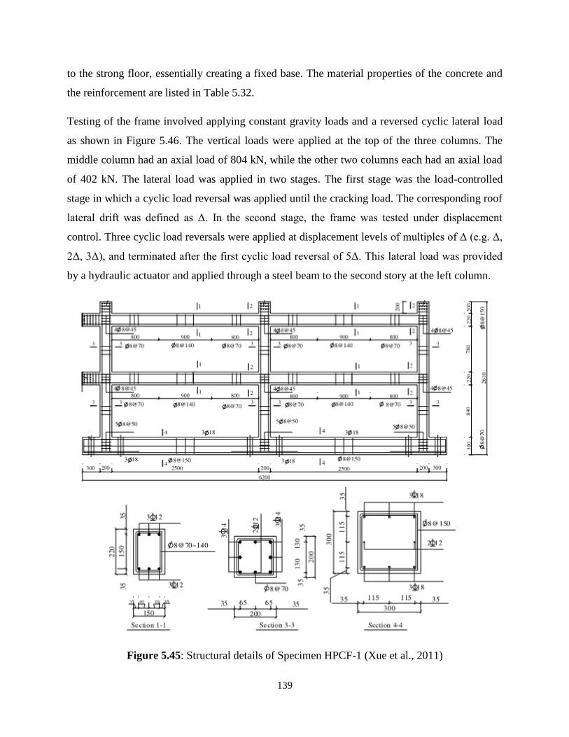
139
to the strong floor, essentially creating a fixed base. The material properties of the concrete and
the reinforcement are listed in Table 5.32.
Testing of the frame involved applying constant gravity loads and a reversed cyclic lateral load
as shown in Figure 5.46. The vertical loads were applied at the top of the three columns. The
middle column had an axial load of 804 kN, while the other two columns each had an axial load
of 402 kN. The lateral load was applied in two stages. The first stage was the load-controlled
stage in which a cyclic load reversal was applied until the cracking load. The corresponding roof
lateral drift was defined as Δ. In the second stage, the frame was tested under displacement
control. Three cyclic load reversals were applied at displacement levels of multiples of Δ (e.g. Δ,
2Δ, 3Δ), and terminated after the first cyclic load reversal of 5Δ. This lateral load was provided
by a hydraulic actuator and applied through a steel beam to the second story at the left column.
Figure 5.45: Structural details of Specimen HPCF-1 (Xue et al., 2011)

140
Figure 5.46: Applied loads on Specimen HPCF-1 (Xue et al., 2011)
Table 5.32: Material properties of Specimen HPCF-1
5.4.2.1 Analytical Modeling
The beams and columns were divided into a number of segments to create the frame model of
the structure. Segment lengths were approximately 100 mm, which was half of the cross-
sectional depth of the column. Figure 5.47 shows the analytical model with loading and support
restraints. There were 171 nodes, 170 members, 9 support restraints and 1 interior joint in the
model. The base of the frame was not modeled explicitly in this model. Instead, Nodes 1, 27 and
53 at the bottom of the columns were restrained in the horizontal, vertical and rotational
directions. The constant gravity loads were modeled with an axial load of 804 kN applied at
Node 52, and axial loads of 402 kN applied at Nodes 26 and 78. A monotonically increasing
displacement was applied at Node 20 in the horizontal direction. The displacement was applied
in 41 load stages with an increment of 1 mm starting from zero displacement. The extension of
the beams and columns were not modeled because otherwise the program would have identified
Node 52 as an interior joint, providing inaccurate predictions.
Bar
Type
Reinforcement Properties
db
(mm)
Fy
(MPa)
Fu
(MPa)
Es
(MPa)
Esh*
(MPa)
εsh*
(x10-3
)
εu*
(x10-3
)
D14 14.0 268.3 373.3 144000 533 10 207
D12 12.0 362.6 506.0 143000 829 10 183
D8 8.0 534.6 594.0 201000 261 10 238
Spec.
Concrete Properties
f’c
(MPa)
Ec
(MPa)
ε’c*
(x10-3
)
HPCF-1 46.9 36100 2.40
*: estimated
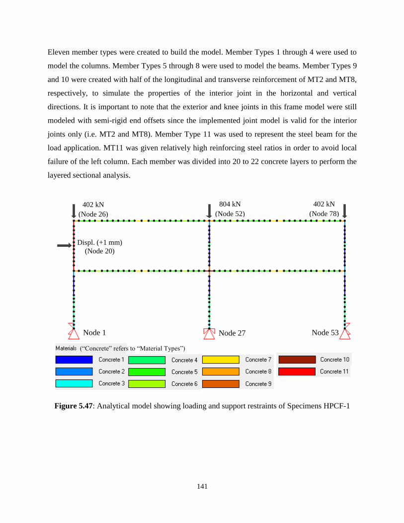
141
Eleven member types were created to build the model. Member Types 1 through 4 were used to
model the columns. Member Types 5 through 8 were used to model the beams. Member Types 9
and 10 were created with half of the longitudinal and transverse reinforcement of MT2 and MT8,
respectively, to simulate the properties of the interior joint in the horizontal and vertical
directions. It is important to note that the exterior and knee joints in this frame model were still
modeled with semi-rigid end offsets since the implemented joint model is valid for the interior
joints only (i.e. MT2 and MT8). Member Type 11 was used to represent the steel beam for the
load application. MT11 was given relatively high reinforcing steel ratios in order to avoid local
failure of the left column. Each member was divided into 20 to 22 concrete layers to perform the
layered sectional analysis.
Figure 5.47: Analytical model showing loading and support restraints of Specimens HPCF-1
804 kN
(Node 52)
402 kN
(Node 78)
402 kN
(Node 26)
Node 1 Node 27 Node 53
(“Concrete” refers to “Material Types”)
Displ. (+1 mm)
(Node 20)

142
5.4.2.2 Comparison of the Analytical and Experimental Responses
The experimental and analytical responses are compared in Figure 5.48. Detailed comparisons of
the response parameters are reported in Table 5.33.
The load-displacement response predicted by V5FBCA had greater strength but lesser ductility
than the observed response. The predicted maximum lateral load was 15% higher than that from
the experiment. In the experiment, the test frame showed good seismic performance and failed in
partial beam sideway mechanism, which involved the formation of plastic hinges at the beam
ends. The initiation of the cracks took place at the column base and mid-span of the beams
before the full vertical loads were achieved. With increasing lateral drifts, cracks formed at the
beam ends and gradually penetrated through the depth of the section. Meanwhile, shear cracks
started forming at the base of the middle column. Vertical cracks due to relatively high axial load
also became visible. The frame structure eventually failed due to the formation of plastic hinges
at column bases. Figure 5.49 shows the flexural failure of the beam end and the shear failure of
the column base.
Figure 5.48: Comparison of base shear versus roof drift response of Specimen HPCF-1
-200
-150
-100
-50
0
50
100
150
200
250
300
-3 -2 -1 0 1 2 3
Ba
se S
hea
r (k
N)
Roof Drift (%)
Experiment (Cyclic)Experiment (Skeleton)V5FBCAVT5

143
Figure 5.49: Failures of Specimen HPCF-1 (Xue et al., 2011)
Table 5.33: Comparison of experimental and analytical results of Specimen HPCF-1
Event First Yielding of Reinforcement Maximum Lateral Load
Results Analysis Experiment Ratio Analysis Experiment Ratio
Lateral Load (kN) 213.3 195.8 1.09 259.1 225.0 1.15
Roof Drift (mm) 13.2 19.9 0.66 28.0 37.8 0.74
Global Stiffness (kN/mm) 16.16 9.85 1.64 9.25 5.95 1.56
The analytical results suggested a similar failure mechanism. Yielding of the column
reinforcement took place at the base of the right column at a roof drift of 0.6%. Meanwhile,
flexural cracks started forming at the beam ends near the column faces on the first story. With
increasing applied lateral loads, the flexural cracks became longer and wider. The frame
eventually failed due to the shear failure at the first story of the east column. Figure 5.50 shows
the deformed shape and cracking pattern of the frame at the end of the simulation. Shear cracks
at the base of the columns were noticeable before the failure of the frame took place. The
compression softening coefficient of the interior joint core was 0.865 at the end of the simulation,
meaning that the interior joint was in a good condition throughout the analysis.
The experimental study did not provide detailed information about the joint core during the test
because the joint failure was not the governing failure mode of the specimen. Damages on the
beam ends and the base of the columns were more severe than the damage in the interior joint.
Therefore, the load-displacement responses predicted by V5FBCA and VecTor5 are nearly
identical. This was because only one of the six joints was modeled using the new joint element.
Even if there had been widespread joint damage, the responses would have been the same due to
the five semi-rigid joints. The observation confirmed that the joint model implementation does
not change the response of frames with minimal joint damage. This study also verified that the

144
program is capable of capturing other failure mechanisms while considering the response of
interior joints.
Figure 5.50: Deformed shape and cracking pattern of Specimen HPCF-1
5.4.3 Ghannoum and Moehle (2012)
An experimental program was conducted to investigate the dynamic collapse of older-type
construction (Ghannoum and Moehle, 2012). The experiment involved testing a one-third scale,
three-story, three-bay frame structure on a shake table. The test frame was constructed with a
center-to-center span of 1780 mm, a story height of 1220 mm and an overall height of 3960 mm
(see Figure 5.51). All beams were 230 mm deep and 150 mm wide, and all columns were 150
mm deep and 150 mm wide. The frame was built integral with four reinforced concrete footings
on top of the shake table. Two of the four columns were designed to represent the older-type
building construction. They had the identical configurations with widely spaced ties with 90-
degree hooks. The other two identical ductile columns were designed in accordance with the
ACI318-08 (2008) requirements for special moment-resisting frames. The purpose of this mixed-
type construction was to delay the collapse of the frame due to the failure of older-type columns.
The design of the frame created a strong-beam, weak-column mechanism. Beam-column joints
were also designed in accordance with ACI318-08 (2008) requirements for special moment-
resisting frames. Therefore, a joint failure was not expected. The material properties of the
concrete and the reinforcement are listed in Table 5.34.
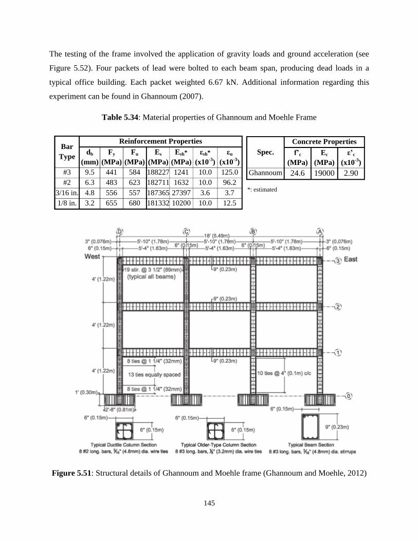
145
The testing of the frame involved the application of gravity loads and ground acceleration (see
Figure 5.52). Four packets of lead were bolted to each beam span, producing dead loads in a
typical office building. Each packet weighted 6.67 kN. Additional information regarding this
experiment can be found in Ghannoum (2007).
Table 5.34: Material properties of Ghannoum and Moehle Frame
Figure 5.51: Structural details of Ghannoum and Moehle frame (Ghannoum and Moehle, 2012)
Bar
Type
Reinforcement Properties
db
(mm)
Fy
(MPa)
Fu
(MPa)
Es
(MPa)
Esh*
(MPa)
εsh*
(x10-3
)
εu
(x10-3
)
#3 9.5 441 584 188227 1241 10.0 125.0
#2 6.3 483 623 182711 1632 10.0 96.2
3/16 in. 4.8 556 557 187365 27397 3.6 3.7
1/8 in. 3.2 655 680 181332 10200 10.0 12.5
Spec.
Concrete Properties
f’c
(MPa)
Ec
(MPa)
ε’c
(x10-3
)
Ghannoum 24.6 19000 2.90
*: estimated

146
Figure 5.52: Applied loads on Ghannoum and Moehle frame (Ghannoum and Moehle, 2012)
5.4.3.1 Analytical Modeling
The beams and columns were divided into a number of segments to create the frame model of
the structure. Segment lengths were approximately 75 mm, which was half of the cross-sectional
depth of the column. Figure 5.53 shows the analytical model with loading and support restraints.
There were 349 nodes, 344 members, 12 support restraints, and 4 interior joint in the model. The
footings were not modeled explicitly in this model. Instead, Nodes 1, 51, 101 and 151 at the
bottom of the columns were restrained in the horizontal, vertical and rotational directions. The
gravity loads provided by four lead packets on each beam span were modeled with two point
loads of 13.34 kN. These loads were applied at 435 mm away from the face of the columns.
Rather than the ground acceleration, a displacement-controlled pushover analysis was employed,
in which a horizontal displacement was applied at the west end of the roof with an increment of
10 mm starting from a zero displacement. Displacements were also applied at the west end of the
first and the second floors with the magnitudes proportional to the height of the floor.
Eight member types were created to build the model. Member Types 1 through 4 were used to
model the columns. Member Type 5 was used to model the beams. Member Types 6 and 7 were
created with doubling the longitudinal and transverse reinforcement amounts of MT1 and MT3,

147
respectively, to employ semi-rigid end offsets of column members. Member Type 8 was created
with doubling the longitudinal and transverse reinforcement amounts of MT5 to employ semi-
rigid end offsets of beam members. Note that the semi-rigid end offsets only applied to exterior
and knee joints, whereas interior joints were modeled with MT1, MT3 and MT5. Each member
was divided into 16 to 24 concrete layers to perform the sectional analysis.
Figure 5.53: Analytical model showing dimensions, loading and support restraints of Ghannoum
and Moehle frame
13.34 kN
Node 1 Node 51 Node 101 Node 151
13.34 kN 13.34 kN 13.34 kN 13.34 kN 13.34 kN
13.34 kN 13.34 kN 13.34 kN 13.34 kN 13.34 kN 13.34 kN
13.34 kN 13.34 kN 13.34 kN 13.34 kN 13.34 kN 13.34 kN
Displ.
(+10 mm)
Displ. (+6.7 mm)
Displ. (+3.3 mm)
(“Concrete” refers to “Material Types”)
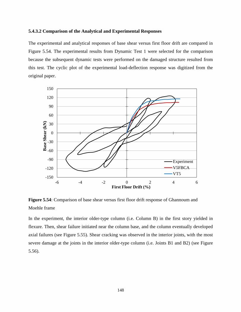
148
5.4.3.2 Comparison of the Analytical and Experimental Responses
The experimental and analytical responses of base shear versus first floor drift are compared in
Figure 5.54. The experimental results from Dynamic Test 1 were selected for the comparison
because the subsequent dynamic tests were performed on the damaged structure resulted from
this test. The cyclic plot of the experimental load-deflection response was digitized from the
original paper.
Figure 5.54: Comparison of base shear versus first floor drift response of Ghannoum and
Moehle frame
In the experiment, the interior older-type column (i.e. Column B) in the first story yielded in
flexure. Then, shear failure initiated near the column base, and the column eventually developed
axial failures (see Figure 5.55). Shear cracking was observed in the interior joints, with the most
severe damage at the joints in the interior older-type column (i.e. Joints B1 and B2) (see Figure
5.56).
-150
-120
-90
-60
-30
0
30
60
90
120
150
-6 -4 -2 0 2 4 6
Base
Sh
ear
(kN
)
First Floor Drift (%)
Experiment
V5FBCA
VT5

149
Figure 5.55: Failures of Ghannoum and Moehle frame (Ghannoum and Moehle, 2012)
Figure 5.56: Damage of interior joints in Ghannoum and Moehle frame (Ghannoum and Moehle,
2012)
Joint C2 Joint B2
Joint C1 Joint B1

150
The load-displacement response predicted by V5FBCA simulated well the experimental
backbone curve in terms of the strength and stiffness. The flexure damage mode was predicted
for this frame, which was similar to the experimental observations. The older-type columns
yielded at a drift of 1.4%. Flexural cracks formed at the base of all columns, as well as the beam
ends near the east column. With increasing lateral drift, flexural cracks extended at the column
bases and propagated through the depth of the beams. Figure 5.57 shows the deformed shape and
cracking pattern of the frame at a drift of 5.2%. Meanwhile, Joints B1 and B2 just reached their
peak strengths, and Joints C1 and C2 were approaching their peak strengths. The predicted
average crack widths in the joint cores ranged from 1.2 mm to 1.6 mm. The experimental
observations indicated that the joints sustained inclined cracking, and spalling in some cases.
Figure 5.57: Deformed shape and cracking pattern of Ghannoum and Moehle frame
5.4.4 Pampanin et al. (2007)
An experimental program was conducted to investigate the efficiency of seismic retrofitting
using fiber-reinforced polymer composites on poorly detailed reinforced concrete frames
(Pampanin et al., 2007). The experiment involved testing of a two-thirds scale, three-story, three-

151
bay frame structure subjected to quasi-static cyclic loading and gravity loads. The frame
structure prior to the retrofit was examined in this study.
The test frame was constructed with a story height of 3000 mm and an overall height of 9000
mm (see Figure 5.58). The beam center-to-center spans were 3000 mm, 1330 mm and 2330 mm.
All beams were 330 mm deep and 200 mm wide. All columns were 200 mm deep and 200 mm
wide. The frame was built integral with a long base above a strong floor serving as the
foundation. The frame was designed in accordance with the design code provisions in the 1970s.
Consequently, no transverse reinforcement was placed in the joint regions. The mechanical
properties of the concrete and reinforcing steel were similar to those typically used in older
structures. The material properties of the concrete and the reinforcement are listed in Table 5.35.
Figure 5.58: Structural details of Pampanin et al. frame (Pampanin et al., 2007)

152
Table 5.35: Material properties of Pampanin et al. frame
Testing of the frame involved applying reversed cyclic lateral loads and constant gravity loads as
shown in Figure 5.59. The gravity loads were simulated with concrete blocks on every beam
span. The lateral loads were applied by three screw jack actuators. The roof displacement was
directly controlled, while displacements on the two lower floors were proportional to the mass of
the concrete blocks and the floor level height. Additional information regarding this experiment
can be found in Pampanin et al. (2002) and Galli (2006).
Figure 5.59: Applied Loads on Pampanin et al. Frame (Pampanin et al., 2007)
5.4.4.1 Analytical Modeling
The beams and columns were divided into a number of segments to create the frame model of
the structure. The length of the column segments was approximately 100 mm, which was half of
the cross-sectional depth of the column. Lengths of the beam segments were approximately 165
mm, which was half of the cross-sectional depth of the beam. Figure 5.60 shows the analytical
model with loading and support restraints. There were 414 nodes, 409 members, 12 support
restraints, and 4 interior joint in the model. The concrete base was not modeled in the analysis.
Bar
Type
Reinforcement Properties
db
(mm)
Fy
(MPa)
Fu
(MPa)
Es
(MPa)
Esh*
(MPa)
εsh*
(x10-3
)
εu*
(x10-3
)
D12 12.0 345 458 176000 1256 10 100
D8 8.0 386 451 176300 722 10 100
D4 4.0 200* 250* 151300 1744 1.32 30.0
Spec.
Concrete Properties
f’c
(MPa)
Ec*
(MPa)
ε’c*
(x10-3
)
Pampanin 14.06 14757 1.91
*: estimated

153
Nodes 1, 74, 147, and 220, located at the base of the columns, were restrained in the horizontal,
vertical and rotational directions. The gravity loads carried by each span are also shown in Figure
5.60. The monotonically increasing lateral loads were modeled in a displacement-controlled
mode. The displacement increments of 6.00 mm, 4.98 mm and 3.12 mm were applied at the roof
level, the second level and the first level, respectively, following the recommendations of Galli
(2006).
Figure 5.60: Analytical model showing dimensions, loading and support restraints of Pampanin
et al. Frame
Node 1 Node 74 Node 147 Node 220
Displ.
(+6.0 mm)
Displ. (+4.98 mm)
Displ. (+3.12 mm)
Each Load = 7.95 kN Each Load
= 7.95 kN Each Load = 6.77 kN
Each Load = 7.95 kN
Each Load
= 7.95 kN Each Load = 6.77 kN
Each Load = 5.60 kN Each Load
= 2.35 kN Each Load = 5.60 kN
(“Concrete” refers to “Material Types”)

154
Eight member types were created to build the model. Member Type 1 was used to model the
columns. Member Types 3 through 5 were used to model the beams. Member Type 2 was
created with double the longitudinal reinforcement of MT1. Member Types 6, 7 and 8 were
created with double the longitudinal reinforcement of MT3, MT4 and MT5, respectively. Note
that there was no transverse reinforcement in MT2, MT6, MT7 or MT8 because the joints were
designed in accordance with the old code provisions. Each member was divided into 20 to 24
concrete layers to perform the sectional analysis.
5.4.4.2 Comparison of the Analytical and Experimental Responses
The experimental and analytical responses of the base shear versus the top floor drift are
compared in Figure 5.61.
Figure 5.61: Comparison of base shear versus top drift response of Pampanin et al. frame
In the experiment, the joint panel regions showed high vulnerability. The structure exhibited an
undesirable global failure mechanism due to strong-beam, weak-column design as shown in
Figure 5.62. Most of the damage concentrated in exterior joints and beam-column interfaces
-60
-40
-20
0
20
40
60
80
-1.8 -1.2 -0.6 0 0.6 1.2 1.8
Base
Sh
ear
(kN
)
Top Drift (%)
Experiment
V5FBCA
VT5

155
through the development of major flexural cracks due to the slip of the longitudinal bars. Few
cracks were observed in the interior joints (see Figure 5.63).
Figure 5.62: Failures of Pampanin et al. frame (Pampanin et al., 2003)
Figure 5.63: Damage of interior joints in Pampanin et al. frame (Pampanin et al., 2007)

156
The load-displacement response predicted by V5FBCA matched well the experimental backbone
response. The program was capable of capturing shear cracking in the beams near the joint
regions, and shear cracking at the base of the columns. In addition, the program predicted the
flexural failure near the mid-span of the first and second story beams in the west bay. As
expected, the program did not predict the major diagonal cracks in the exterior joints due to the
assumption of semi-rigid joints. At a drift ratio of 1.2%, the average crack widths in the interior
joints ranged from 0.2 mm to 0.4 mm, while no cracks were observed in the experiment. Figure
5.64 shows the deformed shape and cracking pattern of the frame at the end of the simulation at a
drift ratio of 1.2%.
Figure 5.64: Deformed shape and cracking pattern of Pampanin et al. Frame
Overall, V5FBCA was able to capture the peak load and the stiffness of the frame structure.
Cracking at the interface of the joints and in the columns were predicted successfully. Despite no
transverse reinforcement used in the joint, the program predicted relative small crack width in
the interior joints, matching the experimental observations.

157
CHAPTER 6
SUMMARY, CONCLUSIONS AND RECOMMENDATIONS
6.1 Summary
The goal of this study was to capture the impact of local joint response on the global response of
frames by implementing an interior beam-column joint model into a previously-developed global
frame analysis procedure, VecTor5. This nonlinear analysis program for two-dimensional
reinforced concrete frame structures was originally capable of providing satisfactory simulations.
The implemented joint element enabled the consideration of joint shear actions and bond slip
effects taking place inside the interior joint cores. The implementation of a joint element allowed
for improved simulations of global load-deflection response and local joint conditions for beam-
column subassemblies and frame structures subjected to monotonic loading conditions.
The analysis procedure with the new joint element was verified with a variety of structures
including nine interior beam-column joint subassemblies and three large-scale frames. As the
main focus of the verification was to determine the accuracy of the implementation and the
improvements over the original VecTor5, the specimens considered covered various material
properties, reinforcing ratios and failure mechanisms. The analytical responses of the specimens
were compared to the experimental responses in terms of load-displacement responses, failure
modes, peak loads, loads at first beam yielding, crack widths, and joint panel shear distortions. In
addition, a parametric study was carried out to investigate the impact of the loading type,
concrete confinement effects, compression softening effects, and bond stress on the analytical
load-displacement responses of the test specimens.
6.2 Conclusions
Based on the results of the analyses performed, the following conclusions and observations are
reached:

158
1. Component-based joint models are suitable for implementation into nonlinear fiber-based
frame analysis procedure, such as VecTor5.
2. Modifications of the global frame analysis procedure are required to facilitate the joint
implementation.
3. Interior beam-column joints can be modeled with the specification of concrete properties,
reinforcing steel properties, joint sectional properties and joint geometric properties.
4. The VecTor5 program had a tendency to overestimate the peak load and initial stiffness
of beam-column joint subassemblies which exhibited significant joint damage due to the
use of semi-rigid joint elements. For the nine interior joint subassemblies modeled, the
ratio of predicted and observed peak load had a mean of 1.25 and a coefficient of
variation of 4.5%.
5. After the new joint element implementation, the peak load and initial stiffness predictions
improved. The predicted failure mechanisms, shear panel distortions, and average crack
widths for the specimens examined showed good correlations with the experimental
results.
6. The improved VecTor5 program with the new joint element showed reasonably good
accuracy in the analysis of beam-column joint subassemblies and frame structures with
interior joints. For the nine interior joint subassemblies modeled, the ratio of the
predicted to observed peak load had a mean of 1.05 and a coefficient of variation of
16.3%.
7. The compression softening model exerts a significant influence on the predicted load-
displacement response. This is concluded from the parametric study of the impact of the
reduction factor due to the compression softening effect.
8. The tensile stresses of reinforcing bars at the joint interface were predicted with
reasonably good accuracy. However, the compressive stresses in reinforcing bars were
not predicted as well as the tensile stresses.
9. The frame structures analyzed showed that VecTor5 considers not only the joint
responses but also the interactions or coupling effects between joints and other parts of
the structure.

159
6.3 Recommendations for Future Research
The following recommendations are made to further improve the modeling of interior joints, and
extend the concept to other types of joints and cyclic loading conditions:
1. In order to achieve improved accuracy and reliability in the analysis, additional work is
required in better describing the constitutive relationships of the joint panel and the bond
slip effects.
2. Reduction factors due to the compression softening effect have significant influence on
the analytical load-displacement response. This study has shown that the compression
softening model by Mitra and Lowes provides satisfactory analytical results. Further
investigations of the effectiveness of other compression softening models would be
useful.
3. The effectiveness of the strut-and-tie model employed for the joint shear panel was not
assessed. Further investigations on this matter require the replacement with other models
such as the Modified Compression Field Theory or the Disturbed Stress Field Model.
4. The sectional analysis of the beam and column members framing into the joint at nominal
flexural strength is currently performed without the consideration of tension stiffening
effect. Further investigation of the impact of the inclusion of tension stiffening models
would be useful.
5. The compressive stresses of reinforcing bars at the joint interface were not predicted well.
This issue is not currently addressed. Further investigations on the reason of this
deficiency are required.
6. The joint formulation is currently only applicable to interior joints. To extend the
formulation to exterior and knee joints, new transformation matrices (see Figure 3.3) are
required to define the equilibrium and compatibility relationships. The size of the
transformation matrices should be 9 x 9 for exterior joints, and 6 x 6 for knee joints.
7. The joint implementation is currently only applicable to monotonic loading. To extend
the formulation to reversed cyclic loading, hysteresis models and damage parameters
must be considered. Additional information is provided in Chapter 4 of Mitra (2007).

160
8. There are currently no explicit joint failure criteria that terminate the program upon the
failure of the joints. Additional work is required to explicitly define the failure criteria to
terminate the program in the case of joint failures.
161
REFERENCES
Alath, S. and Kunnath, S.K., “Modeling Inelastic Shear Deformation in RC Beam-Column
Joints.” Proc., 10th
Conf., University of Colorado at Boulder, Boulder, Colo., May 21-24, ASCE,
New York, Vol. 2, pp. 822-825
Altoontash, A. (2004). “Simulation and Damage Models for Performance Assessment of
Reinforced Concrete Beam-Column Joints.” Ph. D. Thesis, Department of Civil and
Environmental Engineering, Stanford University, California, United States.
Attaalla S.A. and Agbabian, M.S. (2004), “Performance of Interior Beam-Column Joints Cast
from High Strength Concrete under Seismic Loads.” Advances in Structural Engineering, 7(2):
147-157
Celik, O.C. and Ellingwood, B.R. (2008), “Modeling Beam-Column Joints in Fragility
Assessment of Gravity Load Designed Reinforced Concrete Frames,” Journal of Earthquake
Engineering, 12(3), 357-381
Chak, I. and Vecchio, F. J. (2013), "User's Manual of Janus," Online Publication, 211 pp.
< http://www.civ.utoronto.ca/vector/user_manuals/manual5.pdf>
Eligehausen, R., Popov, E.P. and Bertero, V.V. (1983). “Local bond Stress-Slip Relationship of
Deformed Bars under Generalized Excitations.” EERC Report 83/23. Berkeley: University of
California
Elmorsi, M., Kianoush, M.R., and Tso, W.K. (2000). “Modeling Bond-Slip Deformations in
Reinforced Concrete Beam-Column Joints.” Can. J. Civ. Eng., 27(3), 490-505
Fleury, F., Reynouard, J.M., and Merabet, O. (2000). “Multicomponent Model of Reinforced
Concrete Joints for Cyclic Loading.” J. Eng. Mech., 126(8), 804-811
Ghannoum, W.M. and Moehle, J.P. (2012), “Shake-Table Tests of a Concrete Frame Sustaining
Column Axial Failures.” ACI Structural Journal, 109(3), 393-402

162
Ghobarah, A. and Youssef, M. (2001). “Modeling of RC Beam-Column Joints and Structural
Walls.” Journal of Earthquake Engineering, 5(1), 91-111
Guner, S. (2016), “Simplified Modeling of Frame Elements subjected to Blast Loads,” American
Concrete Institute Structural Journal, V.113, No.2, pp.363-372
Guner, S. and Vecchio, F.J. (2012), “Simplified Method for Nonlinear Dynamic Analysis of
Shear-Critical Frames,” American Concrete Institute Structural Journal, V.109, No.5, pp.727-
737
Guner, S. and Vecchio, F.J. (2011), “Analysis of Shear-Critical Reinforced Concrete Plane
Frame Elements under Cyclic Loading,” Journal of Structural Engineering, American Society of
Civil Engineers, V.137, No.8, pp. 834-843
Guner, S. and Vecchio, F.J. (2010), “Pushover Analysis of Shear-Critical Frames: Verification
and Application,” American Concrete Institute Structural Journal, V.107, No.1, pp. 72-81
Guner, S. and Vecchio, F.J. (2010), “Pushover Analysis of Shear-Critical Frames:
Formulation,” American Concrete Institute Structural Journal, V.107, No.1, pp. 63-71
Guner, S. (2008), “Performance Assessment of Shear-Critical Reinforced Concrete Plane
Frames.” Ph.D. Thesis, Department of Civil Engineering, University of Toronto, 429 pp.
Guner, S. and Vecchio, F.J. (2008), “User’s Manual of VecTor5.” Online Publication, 88 pp.
Hakuto, S., Park, R., and Tanaka, H. (1999) “Effect of Deterioration on Bond of Beam Bars
Passing through Interior Beam-Column Joints on Flexural Strength and Ductility.” ACI
Structural Journal, 96(5), 858-864
Hanson, H.W. and Connor, H.W. (1967), “Seismic Resistance of Reinforced Concrete Beam-
column Joints.” Journal of Structural Engineering Division, ASCE, 93(ST5): 533-559.
Hwang, S.J., and Lee, H.J. (2002), “Strength Prediction for Discontinuity Regions by Softened
Strut-and-Tie Model.” Journal of Structural Engineering, ASCE, 128(12): 1519-1526

163
Kim, J. and Lafave, J.M. (2009). “Joint Shear Behavior of Reinforced Concrete Beam-Column
Connections Subjected to Seismic Lateral Loading.” NSEL Report No.NSEL-202. Department of
Civil and Environmental Engineering, Urbana-Champaign: University of Illinois
Lowes, L.N. and Alttontash, A. (2003). “Modeling Reinforced Concrete Beam-Column Joints
Subjected to Cyclic Loading.” J. Strut. Eng. 129(12), 1686-1697
Loya, A. S., Lourenço, D. S, Guner, S., and Vecchio, F. J. (2016), "User's Manual of Janus for
VecTor5," Online Publication, 25 pp. <http://www.utoledo.edu/engineering/faculty/serhan-
guner/Publications.html>
Mander, J.B., Pristley, M.J.N., and Park, R. (1988), “Theoretical Stress-Strain Model for
Confined Concrete.” J. Strut. Eng. 114(8), 1804-1826
Mitra, N. and Lowes, L.N. (2007). “Evaluation, Calibration, and Verification of a Reinforced
Concrete Beam-Column Joint Model.” J. Strut. Eng. 133(1), 105-120
Mörsch, E. (1909). Der Eisenbetonbau, 3rd
Ed., Engineering News Publishing Co., New York
(published in English as “Concrete-steel Construction”).
Noguchi, H. and Kashiwazaki, T. (1992), “Experimental Studies on Shear Performances of RC
Interior Beam-Column Joints.” 10th
World Conf. on Earthquake Engineering, Madrid, Spain, pp.
3163-3168
Pampanin, S., Bolognini, D., and Pavese, A., (2007) “Performance-Based Seismic Retrofit
Strategy for Existing Reinforced Concrete Frame Systems Using Fiber-Reinforced Polymer
Composites”, Journal of Composites for Construction, 11(2), 211-226
Pampanin, S., Magenes, G., and Carr, A. (2003). “Modeling of Shear Hinge Mechanism in
Poorly Detailed RC Beam-Column Joints.” Proc. FIB Symp. Concrete Structures in Seismic
Regions, Federation International du Beton, Athens, Paper No. 171
Park. R. and Dai, R. (1988), “A Comparison of the Behavior of Reinforced Concrete Beam-
Column Joints Designed for Ductility and Limited Ductility.” Bulletin of the New Zealand
National Society for Earthquake Engineering, 21(4), 255-278

164
Pauley, T., Park, R., and Priestley, M.J.N. (1978), “Reinforced Concrete Beam-Column Joints
under Seismic Actions.” ACI Structural Journal, Vol. 75, Iss. 11, 585-593.
Schlaich, J., Schaefer, K., and Jennewein, M. (1987). “Toward a Consistente Design of
Structural Concrete.” PCI Journal, Vol. 32, No. 3, 74-150
Scott, R.M., Mander, J.B., and Bracci, J.M. (2012), “Compatibility Strut-and-Tie Modeling: Part
I - Formulation.” ACI Structural Journal, 109(5), 635-644
Sezen, H. and Moehle, J.P. (2003), “Bond-Slip Behavior of Reinforced Concrete Members.” fib
– Symposium (CEB-FIP); Concrete Structures in Seismic Regions, 6-9 May 2003. Athens,
Greece
Shin, M. and LaFave, J.M. (2004). “Modeling of Cyclic Joint Shear Deformation Contributions
in RC Beam-Column Connections to Overall Frame Behavior.” Structural Engineering and
Mechanics, 18(5), 645-669
Shiohara, H. and Kusuhara, F. (2007), “Benchmark Test for Validation of Mathematical Models
for Non-linear and Cyclic Behavior of R/C Beam-column Joints.” ACI Spring Convention 2007,
Atlanta, United States.
Shiohara H. (2004), “Quadruple Flexural Resistance in R/C Beam-Column Joints” 13th
World
Conf. on Earthquake Engineering, Vancouver, Canada, Paper No. 491
USGS. (2014), “U.S. Geological Survey: Earthquakes with 1,000 or More Deaths 1900-2014”,
http://earthquake.usgs.gov/earthquakes/world/world_deaths.php, Last Accessed September 18,
2016.
Vecchio, F.J. (2000), “The Disturbed Stress Field Model for Reinforced Concrete: Formulation.”
ASCE Journal of Structural Engineering, Vol. 126, No. 9, 1070-1077.
Vecchio, F.J. and Collins, M.P. (1988), “Predicting the Response of Reinforced Concrete Beams
Subjected to Shear using the Modified Compression Field Theory.” ACI Structural Journal, 85,
258-268
165
Vecchio, F.J. (1987), “Nonlinear Analysis of RC Frames Subjected to Thermal and Mechanical
Loads.” ACI Structural Journal, 84(6), 492-501.
Vecchio, F.J. and Collins, M.P. (1986), “The Modified Compression Field Theory for
Reinforced Concrete Elements Subject to Shear.” ACI Structural Journal, Vol. 83, Iss. 2, 219-
231
Viwathanatepa, S., Popov, E.P., and Bertero, V.V. (1979), “Effects of Generalized Loadings on
Bond of Reinforcing Bars Embedded in Confined Concrete Blocks.” Rep. No. UCB/ERRC-79/22
ERRC, Univ. of California, Berkeley, CA
Walker, S.G. (2001). “Seismic Performance of Existing Reinforced Concrete Beam-Column
Joints.” MS thesis, University of Washington, Seattle, Washington.
Walraven, J.C. (1994), “Rough Cracks Subjected to Earthquake Loading.” J. Struct. Eng., 120(5),
1510-1524
Walraven, J.C. (1981), “Fundamental Analysis of Aggregate Interlock.” J. Struct. Div. ASCE,
107(11), 2245-2270
Xue, W., Cheng, B., Zheng, R., Li, L., and Li, J. (2011), “Seismic Performance of
Nonprestressed and Prestressed HPC Frames under Low Reversed Cyclic Loading.” J. Strut. Eng.
137(11), 1254-1262
Zhao, J. and Sritharan, S. (2007), “Modeling of Strain Penetration Effects in Fiber-Based
Analysis of Reinforced Concrete Structures.” ACI Structural Journal, 104(2), 133-141