MODELING FATE AND TRANSPORT OF CRYPTOSPORIDIUM PARVUM

AND ROTAVIRUS IN OVERLAND FLOW

BY

RABIN BHATTARAI

DISSERTATION

Submitted in partial fulfillment of the requirements

for the degree of Doctor of Philosophy in Agricultural and Biological Engineering

in the Graduate College of the

University of Illinois at Urbana-Champaign, 2011

Urbana, Illinois

Doctoral Committee:

Professor Prasanta K. Kalita, Chair

Professor Marcelo H. Garcia

Associate Professor Richard A. Cooke

Associate Professor Timothy R. Ellsworth

ii

ABSTRACT

In the United States, there have been at least 1870 outbreaks associated with drinking water

during the period of 1920 to 2002, causing 883,806 illnesses. Most of these outbreaks are

resulted due to the presence of microbial pathogens in drinking water. Cryptosporidium parvum

(C. parvum) has been recognized as one of the most frequently occurring microbial contaminants

that can cause infection and diarrhea in many mammalian hosts, including humans. About

403,000 of an estimated 1.61 million residents in the Milwaukee area became ill with the

stomach cramps, fever, diarrhea and dehydration caused by the outbreak of C. parvum in 1993. It

was the largest waterborne disease outbreak in documented United States history. Similarly,

rotavirus is the leading cause of death among children around the world. Each year more than

two million children are hospitalized due to rotavirus infection and more than 500,000 children

die from diarrheal disease caused by rotavirus. Past studies have demonstrated that

environmental factors such as rainfall intensity and duration, slope, soil type and surface cover

conditions significantly affect the transport of C. parvum oocyst and rotavirus in surface flow.

Laboratory experiments conducted at the University of Illinois have demonstrated C. parvum

oocysts and rotavirus transport is greatly influenced by climatic and soil-surface conditions like

slope, soil types, soil texture, and ground cover.

The objective of this study was to simulate the fate and transport of C. parvum and

rotavirus in overland flow in different ground cover and slope conditions. Transport of pathogens

in overland flow can be simulated mathematically by including terms for the concentration of the

pathogens in the liquid phase (in suspension or free-floating) and the solid phase (adsorbed to the

soil solid particles like clay, sand and silt). Advection, adsorption, and decay processes have

been considered in the physically-based model. The mass balance equations have been solved

iii

using numerical technique to predict spatial and temporal changes in pathogen concentrations in

two phases. In order to capture the dynamics of sediment-bound pathogen, the Water Erosion

Prediction Project (WEPP) is coupled with the pathogen transport model. Outputs from WEPP

simulations (flow velocity, depth, saturated conductivity and the soil particle fraction exiting in

flow) are transferred as input to the pathogen transport model. Altogether four soil types (Alvin,

Catlin, Darwin and Newberry), four slope conditions (1.5, 2.5, 3.0 and 4.5%), three rainfall

intensities (2.54, 6.35 and 9.0 cm/hr), and three different surface cover conditions (bare, Brome

grass and Fescue) have been used in the experimental investigations. Results of C. parvum and

rotavirus transport from these conditions have been used in calibrating and validating the model

simulation results.

Model simulation results of C. parvum and rotavirus transport through soil surface with

and without any ground cover (bare soil) have produced very good agreement between observed

and predicted results in most cases. Experimental data on pathogen transport showed multiple

peaks in few cases. It was noted that the model results could capture only first observed peak in

pathogen break through curve but could not replicate multiple peaks in pathogen transport that

were found in experimental results. Additionally, there were more parameters used in model

calibration for vegetated surface compared to surface without ground cover. This study provides

both success and challenges of the Cryptosporidium parvum and rotavirus modeling and list

future activities so that a pathogen transport model can be reasonably used under different

climatic and soil conditions.

iv

ACKNOWLEDGMENTS

The successful completion of this dissertation became possible only because of the unrestricted

accessibility, meaningful and result driven guidance and always encouraging nature of my

adviser Prof. Prasanta K Kalita. I express my deep sense of gratitude to Prof. Kalita for his

continuous assistance, valuable suggestions, and encouragement provided throughout the

research. My sincere gratitude also goes to Dr. Richard A. Cooke for his valuable guidance,

support, suggestions throughout the period of my study and also serving as a member of my

doctoral committee. I am grateful to Prof. Marcelo H. Garcia and Dr. Timothy R. Ellsworth for

their cognitive suggestions, critical comments and constructive criticism, and serving as the

members of my doctoral committee.

I would like to acknowledge the valuable support from my research group members Dr.

Paul Davidson, Daniel Koch and Jennifer Trask for providing the necessary data to calibrate and

validate the model that I developed in this study. Supports from the Construction Engineering

Research Laboratory (CERL) and Illinois Department of Transportation are highly appreciated

for providing the research grants which funded my graduate research assistantships. I would like

to extend my gratitude to all my fellow graduate students at the Department of Agricultural and

Biological Engineering, especially Siddhartha Verma, Joseph Monical, Carlos Bulnes Garcia and

Dr. Goutam Nistala for their generous support and cooperation in various stages of this study.

Above all, I wholeheartedly dedicate this thesis study to my beloved parents and loving

brother who are always behind my success. Last but not the least, despite my best efforts and all

the generous help I received, errors may exist. However, any errors that may remain are entirely

my own.

v

TABLE OF CONTENTS

CHAPTER 1: INTRODUCTION ....................................................................................... 1

CHAPTER 2: OBJECTIVES .............................................................................................. 8

CHAPTER 3: REVIEW OF LITERATURE .................................................................... 10

CHAPTER 4: EXPERIMENTAL STUDIES ................................................................... 46

CHAPTER 5: DEVELOPMENT OF A PHYSICALLY-BASED MODEL FOR

TRANSPORT OF PATHOGEN IN OVERLAND FLOW ...................... 58

CHAPTER 6: RESULTS AND DISCUSSION ................................................................ 67

CHAPTER 7: CONCLUSION ....................................................................................... 139

CHAPTER 8: RECOMMENDATION FOR FUTURE WORK .................................... 142

REFERENCES ............................................................................................................... 143

1

CHAPTER 1: INTRODUCTION

After air, water is one of the most important essentials for life. Not only is water necessary for

the digestion and absorption of food, but it also helps to maintain proper muscle tone, supplies

oxygen and nutrients to cells, purges the body of wastes and regulates the body temperature.

Chaplin (2006) has summarized the importance of water in human life as “Liquid water is not a

'bit player' in the theatre of life - it's the headline act”.

Most of the developed world perceives clean drinking water from the tap as an ordinary

and standard part of life, not a luxury. But even today, over one billion people across the world

do not have access to clean water and over two billion people lack access to improved sanitation

(WHO, 2009). About 3.5 million people (including 3 million children) die worldwide due to

water related diseases every year (Prüss-Üstün et al., 2008). Majority of these deaths, about 98%,

occur in the developing countries where water-borne outbreaks are prevalent. Diarrheal illnesses

alone causes more than 1.5 million deaths annually making it worse health threat than cancer or

AIDs in terms of death toll (Prüss-Üstün et al., 2008). A report published by Pacific Institute in

2002 predicts that approximately 135 million people will die worldwide from water related

diseases by 2020 if no action is taken to address basic human needs for safe drinking water

(Gleick, 2002). The report also projects that between 34 and 76 million people will die from

water-related diseases by 2020 even with the accomplishment of Millennium Goals (by 2015,

halve the proportion of people who are unable to reach or to afford safe drinking water)

announced by the United Nations in 2000.

A water source can be contaminated in many ways by municipal sewage, polluted urban

runoff, pesticides and fertilizers from agricultural fields, animal waste from feedlots and farms,

2

industrial pollution from factories, mining waste, hazardous waste sites, spills and leaks of

petroleum products, and industrial chemicals etc. Like the rest of the world, contamination of

water sources by harmful chemicals and infectious pathogens also affects the health of millions

of residents in the United States. In order to monitor the outbreak of water related diseases in

US, the Centers for Disease Control and Prevention (CDC) in partnership with the Council of

State and Territorial Epidemiologists (CSTE), and the Environmental Protection Agency (EPA)

initiated a national surveillance system known as the Waterborne Disease and Outbreak

Surveillance System (WBDOSS) in 1971. As documented by WBDOSS, there have been 794

waterborne disease outbreaks making more than 575,000 people sick from 1971 to 2006. If we

take the annual average for the same duration, about 20 drinking water-related disease outbreaks

are reported to CDC, affecting an average of 15,000 people per year. Center for Disease Control

and Prevention (CDC) has placed water safety threats as category B bioterrorism threats in USA

(CDC, 2009).

The United States has over 300 million acres of land that produces an abundant supply of

low-cost, nutritious food and other products. And, the state of Illinois alone has more than 28

million acres of agricultural land. American agriculture is noted worldwide for its productivity,

quality, and efficiency in delivering goods to the consumer. However, improperly managed,

agricultural activities can affect water quality. The National Water Quality Inventory, published

in 2000, reports agricultural Non-Point Source (NPS) pollution as the leading source for

deteriorating water quality in surveyed rivers and lakes, the third largest source of impairments

to surveyed estuaries, and also a major contributor to ground water contamination and wetlands

degradation (EPA, 2000). Runoff from animal production facilities may contain high levels of

nutrients, solids, and microorganisms that have the potential to degrade the quality of surface

3

water sources. This issue becomes a primary concern when there is a substantial risk for disease

transmission by waterborne microorganisms, especially pathogens. Microbial pathogens present

in agricultural runoff impose a significant hazard on human health when acquired directly via the

fecal-oral route or indirectly as a waterborne contaminant.

Cryptosporidium parvum (C. parvum) is one of those microbial pathogens, which are

found in large quantities in the feces of diseased animals. Cryptosporidium parvum, a protozoan

parasite, is excreted in the form of an oocyst. Livestock and concentrated animal facilities have

been associated with high concentrations of C. parvum. Infected animals have been known to

pass as many as 10 billion oocysts per gram of feces. Therefore, only a few infected animals can

produce enough oocysts to potentially contaminate a large water source (Fayer et al., 2000). The

remarkable infective potential Cryptosporidium is illustrated by the largest outbreak of

waterborne disease in US history in Milwaukee, Wisconsin in the spring of 1993. About 403,000

people were affected from the outbreak, which also caused more than 100 casualties (MacKenzie

et al., 1994; Kramer et al., 1996; Hoxie et al., 1997). Many conventional measures used in water

treatment techniques, such as chlorination, are not very effective in disinfecting the oocyst due to

its resistive nature (LeChevallier et al., 1991). Due to the unique structure of the oocyst, C.

parvum is resistant to diverse environmental conditions and various chemicals that make it a

significant concern from a water quality perspective. As watercourses are the most common

pathways for the oocyst transport, the removal of C. parvum from runoff can contribute to

alleviating water quality and addressing health concerns.

Rotavirus is among the smallest of pathogens but a leading cause of death of children

around the globe. Rotavirus infection kills more than 500,000 children under the age of 5 every

year, most of them in developing countries (Feng et al., 2002). Even in a developed country like

4

the United States, rotavirus was estimated to be the cause of about 60,000 hospitalizations and

37 deaths annually during the period of 1993–2003 Fischer et al., 2007). Apart from human,

rotaviruses have a wide host range including many mammalian species like pigs (Ferrari and

Gualandi, 1986), lambs (Wray et al., 1981), foals (Conner and Darlington, 1980), rabbits

(Conner et al., 1988) and deer (Smith and Tzipori, 1979).

Vegetative filter strips (VFS) is one of the most popular Best Management Practices

(BMP) in controlling the movement of polluted agricultural runoffs into source waters.

Vegetative filter strips are maintained areas of vegetation placed down slope of potential

pollutant sources. The filter strips reduce runoff velocity allowing more water detention on the

surface, which promotes more infiltration into the soil profile, adsorption to the vegetation and

sediment, and deposition of suspended solids. Many studies have suggested that a VFS can be an

effective tool in removing pathogens including C. parvum oocysts and rotavirus from surface

runoff (Brush et al., 1999; Atwill et al., 2002, Trask, 2002, Trask et al., 2004; Davidson, 2007;

Davidson, 2010).

The risk of large microbial pathogenic contamination is not only a human health hazard

but also a potential threat to the continued existence of small to medium-sized dairy farms and

feedlots. To design and develop control mechanisms, microbial transport processes in surface

and near-surface runoff need to be properly understood and quantified along with various factors

that affect pathogen transmission to the environment. While some information exists for C.

parvum oocyst (Brush et al., 1999; Atwill et al., 2002; Tate et al., 2004; Trask et al., 2004) and

rotavirus (Goyal and Gerba, 1979; Davidson, 2007; Davidson, 2010) transport in soil using small

scale experiments hardly any attempts have been made to model transport and fate of oocysts in

surface and near-surface flow conditions. Similarly, no information is available on the effects of

5

various environmental factors such as duration and intensity of precipitation, snowmelt,

vegetation and land-use condition, watershed topography, and actual watershed management

practices on pathogen loads from dairy/cattle farms to the water supply. These factors dominate

pathogen transport rates to the environment (Brown et al., 1980; Medema et al., 1998), and the

information is essential for developing strategies and designing BMP for source control of

microbial pathogens. Otherwise, the risk of water contamination by dairy/cattle farms will

continue unabated, thereby putting cattle and dairy operations at risk.

A model is an abstraction and simplification of a real system. Apart from replicating

present condition, models also allow prediction and simulation of future scenarios, both in time

and space. Hence, models can be both cost-effective and time-saving tool if used appropriately.

In the area of hydrology and water quality, models simulate the natural process of water flow,

sediment movement along with chemical, nutrient and microbial pathogen transport. These

models not only help in addressing a range of environmental problems but also play an important

role in quantifying the effect of human activities on the flow processes. To name few,

Agricultural NonPoint−Source pollution model or AGNPS (Young et al., 1987; Young et al.,

1995; Bingner and Theurer, 2001; Shamshad et al., 2008), Areal Nonpoint Source Watershed

Environment Response Simulation or ANSWERS (Beasley et al., 1980; Connolly et al., 1997;

Bouraoui et al., 2002), CASCade of planes in 2−Dimensions or CASC2D (Ogden and Julien,

2002), Hydrological Simulation Program – Fortran or HSPF (Bicknell et al., 1993), KINematic

runoff and EROSion model or KINEROS (Woolhiser et al., 1990), the European Hydrological

System model or MIKE SHE (Refsgaard and Storm, 1995), and Soil and Water Assessment Tool

or SWAT (Arnold et al., 1998) are few popular water quality models. Generally, these models

are focused on surface water hydrology rather than subsurface hydrology and also require a

6

significant amount of data and empirical parameters for development and calibration. Apart from

SWAT, most of these models can simulate runoff, sediment yield, and nutrient losses within and

from a watershed but not pathogen transport.

Monitoring real-world transport of pathogenic microorganisms such as C. parvum and

rotavirus on a continuous basis is difficult, expensive and not feasible for many water resources

systems. Additionally, there is also a need for the ability to predict the levels of specific

pathogens as a result of non-point sources of contamination. Many waterborne disease outbreaks

have occurred following periods of intense rainfall (Hrudey et al., 2002; Hunter, 2003),

suggesting a link between watershed hydrology and disease transmission. A better understanding

of the connection between microbial occurrence and watershed hydrology is greatly needed.

Since it is very difficult to monitor the influence of several environmental factors on pathogen

fate and transport, modeling can provide a quantitative and consistent approach to estimate

pathogen loading under a wide range of conditions. Models can also predict the extent of

movement along with the time required for the microorganisms to move to the target location.

As noted by Jamieson et al. (2004), there have been few attempts to simulate microbial

pathogen in surface waters at watershed scale such as “loading” models like MWASTE (Moore

et al., 1989), COLI (Walker et al., 1990), and SEDMOD (Fraser et al., 1998). Similarly, models

are also developed to simulate survival and transport of fecal bacteria in receiving waters such as

lakes (Canale et al., 1993) and rivers (Wilkinson et al., 1995) and there also exists model that

incorporate both landscape and in-stream microbial processes like Soil and Water Assessment

Tool (SWAT) (Sadeghi and Arnold, 2002) and a watershed model developed by Tian et al.

(2002). These models simulate the survival and transport of indicator organisms, typically Fecal

coliform. Although overland flow is recognized as the primary transport mechanism of

7

microorganisms to receiving streams in these models, the physical processes involved in the

movement of microorganisms on the land surface has received little attention. Apart from

SWAT, no other models explicitly attempt to partition microorganisms into adsorbed and non-

adsorbed fractions in sediments. Unfortunately, reliable data on bacteria partitioning is currently

not available, which also imposes a challenge to validate SWAT’s partitioning approach. In

current models, sediment-associated microorganism resuspension and deposition rates in streams

are simulated as simple empirical functions of discharge. No attempt has been made to assess the

movement of microorganisms by directly modeling the sediment particles to which they are

attached.

This study intends to bridge the knowledge gap in pathogen transport modeling by

developing a simulation tool for C. parvum oocysts and rotavirus transport in surface and near-

surface flow considering partitioning of pathogens into adsorbed and non-adsorbed fractions.

8

CHAPTER 2: OBJECTIVES

The overall objective of this study is to understand microbial pathogen transport and transport

processes, characterize critical environmental factors affecting microbial transport and control in

runoff and near-surface runoff, and develop a predictive model for microbial transport in surface

and near-surface runoff. The results obtained from this study can be used for translating basic

research results into designing agricultural BMPs that will prevent transport of microbial

pathogens to the water supply. In order to achieve this overall objective, the following specific

research aims were proposed:

1. Review the literatures related to models developed to simulate microbial pathogens

transport processes and characterize the effects of various environmental factors such as

duration and intensity of precipitation, vegetation and land-use condition on overland

(surface) and near-surface (shallow sub-surface) transport of Cryptosporidium parvum

and rotavirus.

2. Develop a predictive model for Cryptosporidium parvum and rotavirus transport in

surface and near-surface flow.

3. Calibrate and validate the model using observed data.

4. Analyze the observed and predicted results and develop recommendation on further use

of the model for designing BMP (such as VFS) to control microbial pathogen transport.

The study also intends to test the following hypothesis regarding Cryptosporidium parvum and

rotavirus transport in surface and near-surface flow:

1. Vegetation reduces pathogen transport drastically by reducing flow velocity providing

more time for pathogens to interact with soil and vegetation surface.

9

2. Rainfall intensity, bed slope and soil type are important factors affecting pathogen

transport in surface and near-surface flow.

10

CHAPTER 3: REVIEW OF LITERATURE

This chapter is divided into 4 sections: section 1 describes about pathogens in general (outbreaks

and regulations); section 2 describes about Cryptosporidium in general (life cycle and

experimental studies); section 3 describes about rotavirus in general (life cycle and experimental

studies); and section 4 provides the details of modeling studies related to all microbial pathogens

including C. parvum.

3.1 Microbial pathogens: an introduction

Potential waterborne pathogenic microorganisms include bacteria, viruses and prions, fungi and

microsporidia, protozoa and helminths (Cotruvo et al., 2004). Many grow in the human or

animal intestinal tract and are transmitted through the feces of infected individuals. Others, such

as prions (e.g. the pathogen causing bovine spongiform encephalopathy, also known as mad cow

disease) have not been ruled out as being capable of causing disease through waterborne

transmission (Cotruvo et al., 2004), although initial estimates suggested negligible risk (Gale,

2001). Fecal pollution of water can result in new infections if the water is not adequately treated.

C.parvum has largely been the pathogen driving drinking water treatment regulations because of

its resistance to conventional treatment (including chlorine disinfection) (e.g. Korich et al., 1990)

and its role in waterborne disease outbreaks in the United States and around the world (Hoxie et

al., 1997; Craun et al., 2006; Karanis et al., 2007), but many other known and emerging

pathogens have been identified.

Zoonotic pathogens (pathogens transmissible between vertebrate animals and humans)

comprise 75% of the emerging infectious diseases in humans. Many of these emerging zoonoses

are transmitted indirectly through water, foods, or environmental contamination (Bolin et al.,

11

2004). Evidence suggests that zoonotic waterborne pathogens will continue to be recognized as

an increasing public health concern worldwide because of a multitude of driving forces that

include changing pattern in water use, climate change leading to severe weather events,

increasingly concentrated livestock operations, and international trade in animal products

(Cotruvo et al., 2004). Pathogens may reemerge because of their ability to adapt, mutate or

recombine in response to changing environmental pressures (Cotruvo et al., 2004). In the United

States, Giardia, Campylobacter, Cryptosporidium, Salmonella, and E. coli have been the most

commonly identified zoonotic agents of waterborne disease outbreaks from contaminated

drinking water (Craun et al., 2004).

Craun et al. (2006) reported that at least 1870 outbreaks were associated with drinking

water, an average of 22.5 per year, during the period of 1920 to 2002. In terms of illness,

883,806 illnesses were reported, an average of 10,648 cases per year during the same period.

During the same period (1920-2002), 1165 deaths were reported, an average of 14 deaths per

year. As shown in Figure 3.1 below, the average annual number of Water borne disease

outbreaks (WBDOs) ranged from a low of 11.1 during 1951–1960 to as many as 32.4 WBDOs

during 1971–1980. The average annual number of illness cases ranged from a low of 1249

during 1951–1960 to a high of 36,162 cases during 1991–2002. In the 12-year period from

1991to 2002, 207 WBDOs causing 433,947 illnesses and 73 deaths were reported; slightly more

WBDOs occurred in non-community water systems (42%) than either community (36%) or

individual systems (22%). During 1991–2002, Giardia (16%) and chemical contaminants (12%)

were two main important causes of WDOs along with a number of other pathogens including

Cryptosporidium (7%), norovirus (6%), E. coli O157:H7 (5%), Campylobacter (3%), and

Legionella (3%).

12

Figure 3.1 Reported waterborne outbreaks, 1920-2002 (Craun et al., 2006).

In 1914, federal regulation of drinking water quality started as the U.S. Public Health

Service set standards for the bacteriological quality of drinking water (USEPA, 1999). This

standard was applicable to water systems which provided drinking water to interstate carriers

like ships, trains, and buses, and only applied to contaminants capable of causing contagious

disease only. These standards were revised and expanded in 1925, 1946 and 1962 by the Public

Health Service. The 1962 standards regulated 28 substances and are considered the most

comprehensive federal drinking water standards in existence before the Safe Drinking Water Act

came into the existence in 1974 (USEPA, 1999). These days, public water systems are regulated

under the Safe Drinking Water Act (SDWA) of 1974, which was amended in 1986 and 1996 and

administered by the U.S. Environmental Protection Agency’s Office of Ground Water and

Drinking Water and its partners. The 1996 amendments required Environmental Protection

13

Agency (EPA) to publish every five years a list of contaminants known or anticipated to occur in

public water systems and possibly needing regulation. Microbial contamination is regulated

under the Surface Water Treatment Rule (SWTR) of 1989 and the Total Coliform Rule (TCR) of

1989. United States Environmental Protection Agency introduced the Interim Enhanced Surface

Water Treatment Rule (IESWTR) on December 1998, which provides additional protection

against C. parvum and other waterborne pathogens.

In 1998, the United States Environmental Protection Agency developed a Drinking Water

Contaminant Candidate List which comprised 60 contaminants and contaminant classes,

including 10 microbial contaminants and groups of related microorganisms and 50 chemicals and

chemical groups (USEPA, 1998). The group of 10 microorganisms included in the list was

Acanthamoeba, Adenovirus, Aeromonas hydrophila, Caliciviruses, Coxsackieviruses,

Cyanobacteria, Echoviruses, Helicobacter pylori, Microsporidia, and Mycobacterium avium

intracellulare. The American Water Works Association Research Division Microbial

Contaminant Committee reviewed the importance of several emerging pathogens for the

drinking water industry in 1999. Three viral, four bacterial, three protozoan microorganisms, and

one set of bacterial toxins were examined (LeChevallier et al., 1999a; LeChevallier et al.,

1999b). They were enteroviruses, calicivirus, Norovirus, and hepatitis A virus; Mycobacterium

avium complex, Helicobacter pylori, pathogenic Escherichia coli, Campylobacter jejuni;

Cyclospora cayetanensis, Microsporidia, and Toxoplasma gondii; and cyanobacteria toxins,

respectively. It should be noted that there are five pathogenic groups of E. coli. A frequently

found strain E. coli O157:H7 is a member of the enterohemorrhagic group (EHEC). Other groups

include enteropathogenic E. coli (EPEC), enterotoxigenic E. coli (ETEC), enteroinvasive E. coli

14

(EIEC), enteroaggregative E. coli (EAggEC), and diffuse adherent E. coli (DAEC) (LeChevallier

et al., 1999a).

Ferguson et al. (2003) have tried to fulfill the knowledge gap concerning precise

mechanism of pathogen transport and provided extensive review of numerous studies related to

fate and transport of surface water pathogens in watersheds. Pathogens considered in the study

were E. coli, Campylobacter, Salmonella, Cryptosporidium and Giardia. The study has also

proposed a conceptual model for pathogen transport in different watershed processes.

It is of critical importance to control or eliminate runoff-mediated contamination of

agricultural watersheds for the preservation of safe water resources and sustainable agriculture.

To design and develop these control mechanisms, microbial transport processes in surface and

near-surface runoff need to be properly understood and quantified. Little information is available

on the environmental or physicochemical factors governing microbial pathogens like C. parvum

and rotavirus transport in surface and near-surface runoff. In case of C. parvum, its unique

biological characteristics and highly resistant nature in the environment makes the environmental

survival and disease transmission issues even more complicated. In order to understand the

transport of C. parvum, knowledge about its biological characteristics, prevalence in the

environment, disease, contamination sources, potential factors associated with transport, the

current removal of C. parvum from drinking water and different model developed to characterize

fate and transport is needed. Therefore, these issues, in addition to previous research using

vegetative filter strips as a control measure for pathogen transport, are discussed.

3.2 Cryptosporidium parvum

Cryptosporidium parvum is a coccidia protozoan from the phylum Apicomplexa, family

Cryptosporidiidae (Fayer et al., 1997). There are eight species of Cryptosporidium that are

15

considered legitimate, though most of the research has focused on Cryptosporidium parvum. The

interest in C. parvum is greater than that of the other seven species because C. parvum has been

identified as the cause of clinical disease in humans and zoonotic infections in livestock, and

other mammals (Robertson and Smith, 1992). C. parvum is a unique parasite found in a very

robust form in the environment. This form, called an oocyst, is resistant to most natural

environmental conditions (Gajadhar and Allen, 2004). This resistance gives the oocyst a long

survival time in the environment and the potential to travel long distances, most commonly

transported in water. Studies have shown that some oocysts can survive up to 32 days at a

temperature of -22oC and still remain viable (Robertson et al., 1992).

3.2.1 Sources of C. parvum

There are numerous sources of C. parvum in the environment; some have bigger impact on water

supplies than others. The impact of livestock on contamination as well as the impact of other

major wildlife that contribute to possible contamination of water courses are discussed in the

next section.

C. parvum can cause gastrointestinal illness in a wide variety of mammals, including

humans, cattle, sheep, goats, pigs, horses, deer, raccoons, opossums, and rabbits (Ungar, 1990).

Hence, the potential for other animals to produce oocysts that infect humans is high. Farm

animals, especially livestock, which include beef and dairy cattle, sheep, horses and pigs, are

susceptible to C. parvum infection. Cattle are thought to be a major source of oocysts among

these groups because of their numbers, distribution, and incidence of infection and also they are

capable of producing up to 10 billion oocysts per gram of feces (Olson et al., 1999; Kuczynska

and Shelton, 1999). Infections have developed in young ruminants around calving times as well

as asymptomatically in adults, usually in the warmer months (Mawdsley et al., 1995; Graczyk et

16

al., 2000). Infection can occur in animals and humans with ingestion of as little as 10 oocysts

from a contaminated water supply (Harter et al., 2000). In 2007, confined beef and dairy cows

produced over 160 million tons of manure in the U.S. (Capper et al., 2009). With this type of

production and the potential for just a few infected cattle to contaminate a large water supply, the

potential for infection is great.

Most birds do not pose a threat to humans because it is unlikely that they carry C.

parvum. An exception to this is gulls, which tend to feed at animal production facilities and

wastewater treatment plants (Fayer et al., 1997). Canadian geese are another bird species that can

carry and produce oocysts (Graczyk et al., 2000). Deer and other ranging animals such as zebras

and buffalo may also be potential reservoirs for C. parvum (Fayer et al., 1997). A study in Spain

that examined the infectivity of small mammals (i.e. rodent and insectivore species) to C.

parvum showed that all types of species became infected during the trial. These findings show

that small mammals may become an important source of oocysts in the absence of humans and

livestock (Torres et al., 2000).

Many studies have looked at the rates of infection among cattle. Graczyk et al. (2000)

studied dairy and beef cattle in Pennsylvania that were allowed to wade and graze near streams

and found that 64% of the farms (n=50) tested positive for the presence of oocysts in at least one

manure sample and 44% were positive in all samples. Livestock were allowed direct access to

watercourses without barriers present (i.e., vegetative filter strips). To compound the problem,

these farms and their manure storage areas are located on a 100-year floodplain and are at risk

for inundation. Starkey et al. (2005) reported that 747 samples, out of the 9914 fecal samples

collected from 39 study farms in Catskill/Delaware watershed of New York City, were found to

17

contain C. parvum. Garber et al. (1994) concluded that with herds over 100 head, virtually all

have been infected with C. parvum at some time in their lifetimes.

3.2.2 Life Cycle of Cryptosporidium

The life cycle of C. parvum consists of several stages followed by a final excretion stage of

mature oocysts into the environment. The initial endogenous stage commences when a host

ingests the oocyst. Sporozoites within the oocyst are released (excysted) from the suture end and

adhere to epithelial cells that line the gastrointestinal tract. For most parasites, excystation

requires reducing internal conditions, exposure to pancreatic enzymes, and bile salts. However,

C. parvum is one parasite that can survive in normal physiological conditions. Once the cell’s

microvilli encapsulate the sporozoites, there is a parasite/host cell relationship. The four

sporozoites from the oocyst form trophozoites, which undergo asexual reproduction (merogony).

After asexual reproduction, six to eight nuclei are formed and mature into a merozoite of type I

meront, a similar structure to the sporozoite. At this point, the type I meront has the capability to

infect another epithelial cell and repeat asexual reproduction producing more merozoites or

undergo sexual reproduction to form a type II meront. The type II meronts formed after sexual

reproduction either become microgamonts or macrogamonts. Microgamonts, which consists of

about 20% of the type II meronts, are thin-walled oocysts that maintain the parasite’s survival

within the host. They are responsible for continuing the infection in the gastrointestinal tract. It is

the fertilized macrogamonts that develop into thick-walled oocysts and are excreted as mature

oocysts in the host’s feces (Fayer et al., 1997). Each mature oocyst has a two-layered outer wall,

contains four sporozoites, and is approximately 5-m in diameter (Clark, 1999). Once the

oocysts are excreted into the environment, they are viable, completely sporulated, infective, and

await a new suitable host. It is at this time that other mammals such as cattle, sheep, and humans

18

can become infected with C. parvum via fecal-oral route. A schematic showing different stages

of C. parvum life cycle is presented in Figure 3.2.

Cryptosporidiosis is the disease caused by C. parvum infection. It was first reported in

cattle in 1971, which caught the interest of the veterinary medical profession (Rose, 1997;

Current and Garcia, 1991). Cryptosporidiosis was first reported in humans in 1976. At present,

cryptosporidiosis has been identified on all continents, excluding Antarctica, totaling at least 95

countries and has been found to be infective to 79 different species of mammals, including

humans (Current and Garcia, 1991; Fayer et al., 1997). This leads to the belief that the

transmission of C. parvum can cross host species barriers quite easily (Current and Garcia,

1991).

Figure 3.2 Life cycle of Cryptosporidium parvum (Current and Garcia, 1991).

19

3.2.3 Transmission between hosts

Animal and zoonotic transmission of C. parvum can occur in different ways. Infection can occur

directly via the fecal-oral route (zoonotic transmission), through waterborne transmission and

possibly with other parasitic protozoa through food-borne transmission (Current and Garcia,

1991; Widmer et al., 1996; Fayer et al., 1997).

Transmission between humans can occur several ways. These include low hygiene levels,

sexual activities and close contact with infants (Rose, 1997). Most commonly, transmission will

occur with younger children (pre-school) because hygiene levels are not yet fully developed.

Outbreaks in settings where children are prevalent, like day care centers, are common (Current

and Garcia, 1991; Mawdsley et al., 1995; DuPont et al., 1995). Transmission can also occur

when caring for infected livestock, zoo animals and domestic animals. Studies have reported that

155 species of mammals have been found to be infected with C. parvum or C. parvum-like

organisms (Fayer, 2004).

Water is thought to be the predominant route of oocysts to expose new hosts (Rose,

1997). There are also various ways that C. parvum can reach watercourses, including direct

leakage to a drainage system from a storage facility or barn, application of contaminated manure

as a fertilizer to agricultural fields, direct runoff from animal production facilities and direct

contamination by animals (Mawdsley et al., 1995; Kuczynska and Shelton, 1999; Graczyk et al.,

2000). Runoff may also occur because of excessive amounts of precipitation or snowmelt. This

form of transport may become more prevalent with shifting rainfall patterns. For instance, the

precipitation trend in the contiguous United States has shown that up to a 20% increase in annual

snowfall and rainfall over the past century (Groisman and Easterling, 1994; Groisman et al.,

2001). Climatologists are also projecting that flooding events will become more severe and

20

happen more frequently (Bates et al., 2008). In addition, treated or untreated discharge from a

water treatment plant may contain oocysts. Untreated water can then be transported to an area

where new hosts come into contact with the oocysts. These areas include recreational waters,

drinking water wells for humans and animals, and bathing areas (Medema et al., 1998).

Fayer et al. (1997) reported that C. parvum oocysts are the most important biological

contaminant in the United States. C. parvum infection is widespread exceeding several million

cases worldwide (Casemore et al., 1997). Higher rates of infection and transmission occur more

frequently in underdeveloped countries. In the developed regions like North America and

Europe, cryptosporidiosis infection rate is between 1 and 3% and is more prevalent in urban

areas with close human contact than in the lower density rural areas. Studies have shown that

about 25-35% of the population in developed countries (including the United States) has had

cryptosporidiosis at some time in their lives (Sureshbabu et al., 2010). Mead et al. (1999)

estimated that there are about 300,000 cases of diarrhea annually resulting from cryptosporidiosis in

the United States. On the other hand, cryptosporidiosis accounts for approximately 10% of cases

of acute diarrheal illness in developing countries (Chen et al., 2002). The higher rate can be

attributed to the lack of sanitary facilities and clean water, as well as crowded housing

conditions. Diarrhoea is the leading cause of death in children younger than five years of age in

developing countries, where Cryptosporidium infection accounts for 30 to 50 percent of those

deaths (Snelling et al., 2007).

3.2.4 Effects of Infection

A majority of reported C. parvum infections have occurred in the gastrointestinal tract. When

infection occurs in the gastrointestinal tract, symptoms will begin to persist anywhere from 2-10

days following infection and generally last 1 to 2 weeks (Current and Garcia, 1991; Fayer et al.,

21

1997; Mawdsley et al., 1996a). Most of those infected experienced multiple symptoms including

watery diarrhea, nausea and vomiting, abdominal pain, mild fever, anorexia, malaise, fatigue and

respiratory problems. Oocyst excretion can last 1 to 4 weeks after most symptoms have subsided.

General feelings of fatigue and malaise may last up to a month after symptoms cease. In

addition, weight loss and dehydration are extremely common when bowel movements are

frequent and voluminous (Fayer et al., 1997; Mawdsley et al., 1996a).

Although majority of reported cryptosporidiosis infections are related to gastrointestinal

track, the infection does not always take place in the intestinal tract. Infections can occur in the

respiratory tract, gallbladder, biliary tree, and pancreatic duct. Respiratory infections in

particular are becoming more common; symptoms include coughing, wheezing, croup,

hoarseness and shortness of breath. Oocysts have been identified in sputum and tracheal

aspirates. Infections in the gallbladder, bile duct, and pancreas have similar symptoms as

intestinal cryptosporidiosis, although diarrhea may not occur (Current and Garcia, 1991; Fayer et

al., 1997). The health implications of cryptosporidiosis at any infection site vary from person to

person and depend on many factors.

The severity of the disease depends on the immunological status or health of the

individual and the amount of oocysts ingested or absorbed at the time of infection (Mawdsley et

al., 1996a; Current and Garcia, 1991; Fayer et al., 1997; Rose, 1997). In a study that was

conducted by DuPont et al. (1995), 29 healthy volunteers were infected with different doses of

oocysts ranging from 30 to 1,000,000. Results from the study showed that 18 people became

infected, mostly from a dose of 100 or more. The data demonstrated that dosage affects the time

and the duration of the oocyst excretion, but not the severity of the disease or symptoms. The

22

mean ID50 (infective dose for 50% of the population) of this particular bovine strain was found to

be 132 oocysts.

Immunocompromised or immunosuppressed people are at high risk for more severe and

potentially life threatening infection because if impaired T cell functions (Rose, 1997).

Immunocompromised people include those that are HIV positive, have cancer, are transplant

patients, are on immunosuppressive chemotherapy, require renal dialysis or have other viral

infections including chicken pox and the measles (Current and Garcia, 1991, MacKenzie et al.,

1994). Because of C. parvum’s ability to autoinfect, the disease takes a much greater toll on the

individuals with an already weakened immune system. The mortality rate for HIV infected

people with cryptosporidiosis is 50% (Rose, 1997). Fluid replacement which is a primarily a

supportive treatment is essential in patients with severe diarrhea. Normally 3 to 6 liters per day

of fluid loss is expected, whereas HIV patients can lose up to 17 liters of fluid per day (Current

and Garcia, 1991).

3.2.5 Environmental Resistance

C. parvum can be a major health concern because of its resistance to many environmental

stresses for long periods of time. Studies have suggested that the oocyst has evolved to survive in

harsh environmental conditions, which is the key factor for its transport and survivability within

the environment (Robertson et al., 1992; Fayer and Nerad, 1996). Its resistance to temperature

and various chemicals has made it a major concern from a public health perspective. Studies

have also shown that oocysts remain infective in both cold and warm water temperatures as well

as after freeze-thaw. A study found that after snap freezing, all oocysts were nonviable;

however, as temperatures were gradually decreased over time to -22ºC, a small percentage of

oocysts were still viable up to 750 hours (Robertson et al., 1992). Fayer and Nerad (1996)

23

examined oocyst viability at room temperature after freezing oocysts at -10, -15, -20, and -70

degrees Celsius (ºC). For all temperatures, oocysts were viable from 5 to 168 hours except for at

-70ºC. For a temperature of 5ºC, all oocysts were viable for 168 hours. This may allow extended

survival in surface waters during the winter season. Not only can oocysts survive under low and

freezing conditions, they are also viable in warm temperatures. It has been shown that oocysts

can survive in warm water temperatures from 25 to 64ºC (Fayer, 1994). However, the survival

time of oocysts in warm water is much lower than that in cold-water temperatures. A study by

Olson et al. (1999) showed the effects of temperature on oocyst viability in various media. It was

found that at -4 and 4ºC, oocysts remained infectious for more than 12 weeks in water and

autoclaved soil, whereas oocyst survival in cattle feces varied from more than 12 weeks at -4ºC

to 8 weeks at 4ºC. Oocyst survival was less at 25ºC than at -4 and 4ºC. Even though similar

results were reported in soil and cattle feces for various temperatures, water still provides the

best survival medium for C. parvum oocysts in the environment. Therefore, even at low

temperatures, oocysts can be transported in runoff to water sources causing a major risk of

contamination. Unlike other pathogens, C. parvum can remain viable under a variety of

environmental conditions.

The size and structure of the oocyst is another key survival characteristic of C. parvum.

Due to the small size, near neutral buoyancy and negative surface charge resulting in low

hydrophobicity, oocysts can remain suspended in water with the potential to travel long distances

(Drozd and Schwartzbrod, 1996; Walker et al., 1998). Medema et al. (1998) found that both free

and attached oocysts remained in suspension due to their relatively slow settling velocities over

larger particle sizes, thus increasing the chances of transport in water. The outer membrane

structure of the oocyst wall may also change its chemical composition over time increasing its

24

survival rate in the environment (Brush et al., 1999). The structure and composition of the oocyst

also prevents inactivation by various chemical treatments. Many chlorine-based chemicals such

as chlorine, monochloramine, and chlorine dioxide at typical applied concentrations and

conventional treatment disinfection times have little effect on oocyst inactivation (Fayer et al.,

1997). Therefore, conventional drinking water treatment alone cannot guarantee the complete

inactivation of the oocysts from drinking water supplies, thus increasing the risk of disease

transmission.

3.2.6 Cryptosporidium parvum transport studies

Many studies have looked into the biological characteristics of C. parvum since its discovery.

However, extensive research on C. parvum did not commence until there were several reported

major outbreaks of human infection, especially the Milwaukee outbreak in 1993. Since that time,

many studies have investigated various environmental factors affecting oocyst viability such as

temperature, chemical disinfectants, and survival in different media, but characteristics of oocyst

transport within the watershed are limiting (Robertson et al., 1992; Fayer, 1994; Olson et al.,

1999; Bukhari et al., 2000; Davies et al., 2003; Davies et al., 2004; Kaucner et al., 2005;

Ferguson et al., 2007a). Similarly, several studies have been studied the vertical transport of C.

parvum with and without vegetation. Brush et al. (1999) measured the vertical transport of C.

parvum through three different media. The results indicated that there was significant removal of

C. parvum from the sand followed by glass and shale. Harter et al. (2000) also measured the

vertical transport of C. parvum using three different sands and two pore velocities representing a

sandy aquifer and saturated soil following a heavy rain storm event. It was found that medium

sands retained the greatest percent of oocysts within the soil column. Another study investigated

vertical transport of C. parvum using perennial ryegrass vegetation and three soil types: silt-

25

loam, clay-loam, and loamy sand (Mawdsley et al., 1996a). The study showed that oocysts were

found in the subsurface flow for the silt-loam and clay-loam but not for the loamy sand. The

remaining oocysts in the soil were still viable for transport in subsurface and overland flow. Even

though studies have shown that there is a potential risk of groundwater contamination by vertical

transport of oocysts, the potential migration of oocysts through soil seems to be small and much

lower than bacteria and viruses. This is mainly due to the larger size and adsorption properties of

the oocysts to soil particles (Mawdsley et al., 1996a). Vertical transport of C. parvum causing

groundwater contamination is an issue, but most contamination has resulted from surface water

sources, indicating overland flow as the major source of oocysts posing a greater public health

risk. Mawdsley et al. (1996b) studied the vertical and horizontal movement of C. parvum using

three soil-tilting beds after simulated rainfall. The beds were placed at a 7.5% slope and

contained silty clay-loam with perennial ryegrass. The runoff and leachate analyzed for oocyst

concentration indicated that movement of the pathogen lasted for at least 21 days in surface

runoff and in one case for 70 days for subsurface flow. The difference in oocyst transport times

was explained by the variation of the intact soil cores taken from the field. For two of the tilting

soil chambers, more water volume was lost as subsurface flow than surface runoff while the third

soil chamber had approximately the same volumes from surface and subsurface flow. They

suggested the need for further studies using different slopes, varying the distance of application,

and different methods of application to enhance understanding of oocyst transport in overland

flow.

Atwill et al. (2002) examined the efficiency of vegetated buffer strips to remove C.

parvum from surface and shallow subsurface flow using simulated rainfall rates of 15 or 40

mm/h. The experiments were conducted using buffers set at 5 to 20% slope having 85 to 99%

26

Fescue cover with soil textures of either silty clay (19:47:34 sand-silt-clay), loam (45:37:18), or

sandy loam (70:25:5). One of the findings of the study was vegetated buffers constructed with

sandy loam soil (or higher soil bulk densities) were less effective at removing C. parvum

compared to buffers constructed with silty clay or loam soil. The study also concluded that a

vegetated buffer strip comprised of similar soils at a slope of ≤20% and a length of ≥3 m should

function to remove ≥99.9% of C. parvum oocysts from agricultural runoff generated during

events involving mild to moderate precipitation. Trask (2002) studied the effects of ground cover

conditions (bare and vegetated surfaces), slopes and rainfall intensities on C. parvum oocyst

transport in overland and near-surface (shallow subsurface) flow using a horizontal tilting soil

chamber in a controlled laboratory environment. Oocyst transport was investigated for three

slope conditions (1.5, 3.0, and 4.5%) in conjunction with two rainfall intensities (2.54 and 6.35-

cm/hr). Results from the study the surface runoff from the vegetated surface had much lower

total percent recoveries of oocysts than those from the bare-ground conditions for all slope and

rainfall conditions. McLaughlin (2003) studied the adsorption kinetics of C. parvum with

individual soil particles (sand, silt and clay) and vegetation. Using a Coulter Counter and

photomicrographs, soil adsorption were conducted which indicated that oocysts primarily adhere

to or become entrapped within aggregating clay particles and do not adhere substantially to either

silt or sand. Results from the vegetation adsorption experiment showed that the oocysts were

transported more readily on bare soil than vegetated soil. Koch (2009) carried out a series of

small scale laboratory experiments to investigate the effect of vegetation, slope and rainfall

intensity on surface and near-surface transport of C. parvum. The experiments were performed at

3.0% slope and 90 mm/hr rainfall intensity and 2.5% slope and 65 mm/hr intensity. The study

reported that the oocyst recovery in runoff was substantially lower from the vegetated surface

27

condition when compared to those from the bare surface condition for all the cases. Davidson

(2010) examined the kinetics of C. parvum transport in overland flow with the help of series of

small scale laboratory experiments. For the transport studies, three soil types were tested (Catlin

silt-loam, Alvin fine sandy-loam, Darwin silty-clay) with and without vegetation cover. The

results from bare soil experiments showed that a higher recovery of C. parvum oocysts from the

Alvin soil compared to other soil types and vegetation greatly reduced the recovery of infective

oocysts, in addition to delaying the time to the peak recovery.

3.3 Rotavirus

Rotavirus is 65-75 nm in diameter which makes it one of the smallest microorganisms (Ansari et

al., 1991). It belongs to the family Reoviridae and causes inflammation of stomach and

intestines, the medical condition commonly known as gastroenteritis. The rotavirus infection

causes severe watery diarrhea, often with vomiting, fever, and abdominal pain (CDC, 2011). The

virus is the leading cause of severe diarrhea in infants and the most frequently detected pathogen

in children under two years of age in developing countries. The virus accounts for about 5% of

all deaths among children less than five years of age and about one-third of deaths from diarrhea

around the world. It is also estimated that almost every child around the globe has been infected

with rotavirus at least once by the age of three (Velázquez et al., 1996; Feng et al., 2002). The

rates of infection are similar in developed and developing countries but the severity of rotavirus

infections differs between those two settings. Improvements in clean drinking water supplies and

good hygiene are unlikely to prevent the infection since they have little effect on the

transmission of infection (Dennehy, 2008). Although the mortality rates are low in developed

countries, rotavirus infections account for more than 500,000 deaths annually in young children

primarily in developing countries (Bishop, 1996; Feng et al., 2002). In addition, rotavirus causes

28

approximately 111 million episodes of gastroenteritis requiring only home care, 25 million clinic

visits and 2 million hospitalizations each year (Parashar et al., 2003). Based on the studies

published between 1986 and 1999, it was estimated that rotaviruses caused approximately 22%

of childhood diarrhea hospitalizations worldwide (Parashar et al., 2003). However, this

proportion increased to 39% from 2000 to 2004, as reported by Parashar et al. (2006).

Taxonomically, rotaviruses are classified into seven groups: A, B, C, D, E, F and G

(Santos and Hoshino, 2005). Rotavirus A is the most common among them and causes more than

90% of infections in humans. Although the first infection of rotavirus can be fatal in children,

immunity develops with each infection and subsequent infections are less severe (Linhares et al.,

1988). A study showed that intestinal mucosal IgA responses are responsible for protecting

immunity against rotavirus reinfection (Feng et al., 2002).

Because of the large numbers of rotavirus infections around the world, researchers started

to develop a vaccine against rotavirus infection in 1990s. RotaShield, the first rotavirus vaccine

developed by Wyeth, was licensed for use in the United States in 1998. Clinical trials of the

vaccine in the United States, Finland, and Venezuela reported the vaccine to be 80 to 100%

effective at preventing severe diarrhea caused by rotavirus A. Although these trials also showed

no statistically significant serious adverse health effects, the vaccine was withdrawn from the

market in 1999 when it was discovered that the vaccine may have contributed to an increased

risk for intussusception, or bowel obstruction, in one of every 12,000 vaccinated infants. The

experience provoked debate about the relative risks and benefits of a rotavirus vaccine (Bines,

2006). Recently two live oral rotavirus vaccines (RotaTeq and Rotarix) have been recommended

by the WHO for inclusion into the national immunization programs of countries worldwide in

2009 (Patel et al., 2009).

29

As reported by McNulty (1978), the name “rotavirus” was proposed by Flewett et al.

(1974), although the first case of rotavirus infection was documented by Mebus et al. (1969).

Rotavirus infection is very common in humans (Flewett et al., 1973; Bishop et al., 1974;

Middleton et al., 1974; Bishop, 1996; Feng et al., 2002; Parashar et al., 2003, Parashar et al.,

2006) and calves (Mebus et al., 1969; Woode et al., 1974; McNulty and Logan, 1983). In

addition, rotavirus infections have been detected in other mammals including pigs (Rodger et al.,

1975; Woode et al. 1976; Ferrari and Gualandi, 1986), lambs (McNulty et al., 1976; Snodgrass

et al., 1977; Wray et al., 1981), foals (Flewett et al., 1975; Conner and Darlington, 1980), rabbits

(Bryden et al., 1976; Conner et al., 1988) and deer (Tzipori et al., 1976, Smith and Tzipori,

1979) making it a wide-spread infectious agent.

3.3.1 Rotavirus life cycle

Rotaviruses have a complex architecture with double stranded RNA. Microscopic

analyses reveal that they consist of three concentric capsid layers surrounding a genome of 11

segments of double-stranded RNA (Feng et al., 2002). The double stranded RNA (dsRNA) in

rotavirus can be separated into eleven distinct bands by gel electrophoresis. Each of these eleven

distinct bands represents a distinct rotavirus gene that is responsible for synthesis of a single

structural or non-structural viral protein (Estes, 1990). These doube stranded RNA also serve as

templates for the synthesis of the segmented double-stranded RNA (dsRNA) genome (Silvestri et

al., 2004).

The complete infectious particle is composed of six structural proteins assembled as a

triple layer as shown in Figure 3.3. The inner core of virus proteins 1, 2, and 3 (VP1, VP2, VP3)

contains the genetic information in the form of 11 double-stranded RNAs along with the

enyzmes necessary for replication. This is protected by a second shell of VP6, the group antigen

30

that defines a rotavirus as being group A, B, C, etc. The outer shell carries the antigens involved

in protective immunity. The VP4 is the spike protein involved in cell attachment. A glycoprotein,

VP7, is the dominant target of the antibody response. Immunity against VP4 or VP7 is protective

(Shaw, 2006). Group A rotaviruses have been further subdivided on the basis of antigens on VP6

(subgroup I, II), on VP7 (G-types), and on VP4 (P types). Human infections with Groups A, B,

and C viruses have been recorded. Most severe acute diarrhea in children is caused by

rotaviruses of Group A, subgroups I or II, G types 1-4, and P types 1A (Bishop, 1994) or 1B

(Bartlett et al., 1985).

Figure 3.3 The triple-layered particle rotavirus virion (Shaw, 2006).

The rotavirus replication cycle is cytoplasmic as the cycle completes within cytoplasm of

the cell (Estes, 1990). Figure 3.4 shows a simplified life cycle, in which the features critical to

understanding genetics are emphasized (for simplicity, only one of the 11 genome segments is

shown). Upon entry of the virion, the outer capsid is removed which activates the virion-

associated transcriptase. The resulting mRNAs function either as templates for replication of

31

progeny genomes or as messengers for translation into protein. Subviral particles are formed that

contain a mixture of structural and nonstructural proteins, together with one copy of each of the

11 template RNAs after sufficient viral protein is translated. In this cycle, polymerase activities

and dsRNA are always particle-associated and mRNA is the only viral nucleic acid that is free

for genetic interaction (Ramig, 1997).

Figure 3.4 Essential elements of the rotavirus life cycle (Ramig, 1997).

3.3.2 Rotavirus transmission

Rotavirus transmission occurs when a new host comes in contact with contaminated stool

and the pathogen is ingested orally. This is known as a fecal-oral route of transmission. Direct

contact with contaminated surfaces and ingestion of contaminated food or water are two most

frequent pathways of transmission. Factors such as the large number of virus shed by infected

mammals, the very low infectious dose required, and a high degree of resistance to physical

inactivation make the transmission easily spreadable through environmental sources. Rotaviruses

are resistant to environmental stresses and they can survive up to four hours on human hands, 10

32

days on solid, dry surfaces and for weeks on wet surfaces and water (Ansari et al., 1988; Ansari

et al., 1991; Sattar et al., 1984). The rapid nature of rotavirus transmission has been reported by a

number of studies (Foster et al., 1980; Kapikian and Chanock, 1985; Santosham et al., 1985).

It has been reported that rotaviruses can be highly infectious when transmitted within the

same species. Replication within the intestinal tract can result in shedding of 1010

plaque forming

units (PFU) per milliliter of feces (Ansari et al., 1991). The infectious dose for the human small

intestine has been reported as approximately 1 PFU per milliliter (Graham et al., 1987).

Although rotaviruses are generally species-specific, cross-species transmission is also possible

(Cook et al., 2004). Transmission of animal rotavirus to humans is possible because human

infection with rotavirus mutants possessing bovine (or occasionally porcine or avian) genes has

been recorded in Italy, India, Indonesia, Finland, Thailand and the U.S. (Nakagomi and

Nakagomi, 1993).

3.3.3 Rotavirus in the environment

It should be noted that there are more than 120 different virus types that are known to be

excreted in human feces by infected persons and not all of them are pathogenic. Studies have

reported that a number of human enteric viruses may be present even in treated wastewater

effluents (Gerba et al., 1975; Hoadley and Goyal, 1976), suggesting that the application of

wastewater on land may spread the contamination of viruses. The different soil type may exhibit

different virus adsorption characteristics but the effects of different soil type on of viruses during

land treatment of wastewater have not been studied extensively. Similarly, very little is known

about the survival or fate of human viruses applied to the soil or vegetation. Because of their

size, viruses migrate vertically, resulting in groundwater contamination if they are not retained

33

by the soil or vegetation. In fact, few studies have reported the detection of enteroviruses in

groundwater after land treatment (Schaub and Sorber, 1977; Vaughn et al., 1978; Wellings et al.,

1974; Wellings et al., 1975). A study by Abbaszadegan et al. (2003) found that about one-third

of the groundwater drinking wells, out of 448 sites across 35 states, contained human pathogenic

enteric viruses.

Goyal and Gerba (1979) studied comparative adsorption pattern of a number of human

enteroviruses, rotaviruses and bacteriophages to nine different soil types was studied. They

reported that greater than 90% of all viruses adsorbed to a sandy loam soil except echovirus types

1, 12, and 29 and a simian rotavirus (SA-11), which adsorbed to a considerably lower degree.

The study also observed a great deal of variability between adsorption of different

strains of

echovirus type 1, indicating that viral adsorption to soils is highly strain dependent. The

adsorption was found to be influenced also by soil type, in addition to being dependent

on type

and strain of virus. Thus, soils having a saturated pH of less than 5 were generally good

adsorbers. Sagar and Gerba (1979) studied the effect of soil characteristics on different virus

strains. They found that the nature of virus adsorption to soil is highly dependent on the strain of

virus. The variability in the configuration of proteins in the outer capsid of the virus can

influence the net charge on the virus. The net charge on the virus would affect the electrostatic

potential between virus and soil, and thereby could influence the degree of interaction between

them. They also reported that a low soil pH (below 5) appeared to favor virus adsorption of all

the viruses studied. In addition, they found that percent clay, percent sand, percent organic

matter, total phosphorus, resin-extractable phosphorus, total iron, total aluminum, exchangeable

aluminum, and exchangeable magnesium all influenced virus adsorption.

34

In another study, LaBelle and Gerba (1979) investigated the adsorption of enteric viruses

estuarine sediment. Their finding suggested that the viruses are dependent upon the sediment

particle for transport. The study concentrated primarily on clay sediment particles because clay

sediments are the slowest to settle and more easily transported due to the smaller size and mass.

However, the study from Davidson (2007) suggested that rotavirus preferentially interacts with

sand particles. Although some interaction was observed with clay particles, the extent of

interaction was very less as compared to sand particles. Therefore, if rotavirus is bound to the

much larger sand particles, the opportunity for transport is greatly reduced.

3.4 Microbial pathogen transport fate and transport modeling

A model can be defined as an abstract representation of an item or a concept which help us better

understand real world systems. Models can be broadly divided into two categories: physical and

mathematical. A physical model is one that physically represents an object. In most cases, the

physical model either zooms in or zooms out the real object to better understand the different

phenomenon associated with it. In contrast, a mathematical model doesn’t have any physical

presence and uses mathematical language to describe the behavior of a system. In hydrology,

there exist different types of mathematical models based on their formulation. A hydrologic

model can be classified into either lumped or distributed based on spatial discretization. A model

treats a watershed as a single homogeneous element while a distributed model divides the

watershed into many small units such as grid cells. Similarly, a model can be classified into

event-based, continuous time, and large time-scale model based on time scale. Based on solution

techniques, models can be classified as analytical, numerical, and or analog solution model.

Based on the way different hydrologic processes are represented in a model, it can be further

35

classified into data-driven or process-based model. Data-driven models, also known as black-box

models, are usually driven by the raw or processed data and the formulation may not be

conceptually supported by the mechanism of the phenomenon under consideration (Elshorbagy

and Ormsbee, 2006). Process-based models, also known as mechanistic or physically-based

models, describe different processes associated with the phenomenon under consideration and

are parameter-intensive in general.

During the last two decades, computer simulation models for water quality have been

developed to simulate numerous components of pollution from watersheds. These components

include surface runoff, sediment, nutrients, and pesticides. However, little has been done to

address fate and transport of pathogens from watersheds. It is a common practice where

pathogens like fecal coliform bacteria are considered to be associated with surface water flow

and flow-associated constituents like pathogens are assumed to be accumulated on the land

surface until the occurrence of a rainfall event (Paul et al., 2004). Pachepsky et al. (2006) have

reviewed the status and challenges in modeling the fate and water transport of manure-borne

pathogens in the environment. The study included models for the pedon, the hillslope, and the

watershed scales. Jamieson et al. (2004) have reviewed current approaches in modeling the

microbial quality of surface waters at watershed scale. The study has reviewed “loading” models

like MWASTE (Moore et al., 1989), COLI (Walker et al., 1990), and SEDMOD (Fraser et al.,

1998). Similarly, other models developed to simulate survival and transport of fecal bacteria in

receiving waters such as lakes (Canale et al., 1993) and rivers (Wilkinson et al., 1995) have been

included in the study along with models that incorporate both landscape and in-stream microbial

processes like Soil and Water Assessment Tool (SWAT) (Sadeghi and Arnold, 2002) and a

watershed model developed by Tian et al. (2002). These models simulate the survival and

36

transport of indicator organisms, typically FC. Moore et al. (1989), Fraser et al. (1998) and Tian

et al. (2002) all estimate surface transport of bacteria using simple empirical equations which

relate bacteria transport to runoff rate or depth. The empirical transport equations within these

models have not been well tested and validated. The empirical transport parameters have no

physical basis and must be obtained through calibration. The model which have been developed

in past for modeling bacterial fate and transport to the streams such as the revised Agricultural

Runoff Model (ARM II): Animal Waste Version (Overcash et al., 1983), UTAH State (Springer

et al., 1983); MWASTE (Moore et al., 1989); COLI (Walker et al., 1990); Hydrologic

Simulation Program Fortran - HSPF (Bicknell et al., 1997); Spatially Explicit Delivery Model –

SEDMOD (Fraser et al., 1998); and PROMISE and WATNAT (Medema and Schijven, 2001)

have not proven to very effective tool as most of them have limitation in their capabilities.

In 2000, a microbial sub-model was developed and added to the Soil and Water

Assessment Tool (SWAT) to address fate and transport of both more persistent and less

persistent fecal bacteria (Neitsch et al., 2002; Sadeghi and Arnold, 2002). Currently for

hydrologic simulations, a significant amount of research is being done using the SWAT model

because it appears to be the most inclusive of the numerous variables needed to make accurate

predictions of hydrologic systems. A microbial sub-model considers sources of bacteria and their

fate and transport (Sadeghi and Arnold, 2002) and it has been in a continual development process

since that time. The most recent update was released in 2005 (Neitsch et al., 2005).

Tian et al. (2002) developed and applied a modeling system for assessing microbial

contaminants like fecal coliform on animal-grazed farmlands. The model identified the sources,

sinks, transport processes, and fate of E. coli contaminants in catchments and associated streams

including grazing location, land topography, distance to a nearby stream, distance through the

37

stream network to the outlet, population dynamics on the land surface, in flow, and on

streambeds. The model applies the principles of conservation of mass balance on grid cells on

land surfaces and networked stream segments. In order to improve the prediction of the effects of

different land management strategies on the fecal contamination of waterways, the model

characterizes the movement of fecal contaminants from land to streams and in-stream

mobilization. The model was applied to a hill land catchment with an area of 140 ha,

predominantly used for animal grazing. The sensitivity of the model predictions was analyzed for

effect of stock rate (grazing intensity), attenuation rate, and flow volumes and it was found that

the controlling diffusion rate and E. coli rate per pat were the most sensitive parameters. The

authors concluded that further experiments were required to expand the model's functionality for

covering more mitigation options.

Collins and Rutherford (2004) developed a model to predict concentrations of the fecal

bacteria indicator E. coli in streams and applied the model to a small grazed watershed of 259

hectare area in New Zealand. In order to estimate E. coli inputs to the catchment, a daily record

of grazing livestock was used and transport of bacteria to the stream network was simulated

within surface and subsurface flows including in-stream processes of deposition and entrainment

and die-off on land and in water. Although the authors reported that uncertainty existed with a

number of the processes represented in the model, it model broadly reproduced observed E. coli

concentrations in the hill-country catchment grazed by sheep and beef cattle. They also reported

that the model was sensitive to the amount of excretion direct to streams and seepage zones

along with the distance over which surface runoff delivered bacteria to a stream. The study

concluded that riparian buffer strips may improve bacterial water quality both by trapping of

bacteria by the riparian vegetation and by eliminating livestock defaecation in and near streams.

38

Haydon and Deletic (2006) developed two conceptual continuous pathogen models and

evaluated them using E. coli as a pathogen indicator to model pathogen discharges from three

catchments in Australia. The first model, known as the EG model, included surface and

subsurface pathogen transport processes by means of wash-off and loss equations and an existing

hydrologic model (SimHyd) model was coupled with. For flow simulation, EG model was

coupled to an existing hydrologic model (SimHyd). The second model, named ASP, was simpler

than EG as it took into account only surface pathogen transport processes. To drive pathogen

transport, EG model was coupled to a stormflow-baseflow separation model. Both the models

were calibrated and validated using baseflow and storm event E. coli concentrations measured at

three dissimilar catchments from southern Australia. The model results comparison showed that

the prediction of pathogen peak concentrations by the EG model was reasonably better than

those from ASP model.

Wu et al. (2009) developed, calibrated, and validated a watershed scale Escherichia coli

fate and transport model. Escherichia coli densities in water and sediments from the Blackstone

River Watershed, Massachusetts, were measured at three sites for a total of five wet weather

events and three dry weather events covering three seasons. Results showed that there were

significant correlations between E. coli and total coliforms in water and sediments. In addition,

E. coli concentrations in water were weakly correlated with sediment particle size and sediment

concentrations. A hydrologic model, WATFLOOD⁄SPL9 (Kouwen and Mousavi, 2002), was

used to predict the temporal and spatial variation of E. coli in the Blackstone River. The rapid

rise of stream E. coli densities was more accurately predicted by the model with the inclusion of

sediment resuspension, thus demonstrating the importance of the process.

39

Parajuli et al. (2008) applied SWAT model to explore effectiveness of vegetative filter

strip (VFS) lengths applied at the edge of fields to reduce non-point source pollution in the

Upper Wakarusa watershed in northeast Kansas. The study tested the effectiveness of VFS

lengths (0, 10, 15 and 20 m) for reducing sediment and fecal bacteria concentration in overland

flow and also ranked sub-watersheds based on sediment and fecal bacteria contribution of each

sub-watershed. They reported that the 15-m VFS reasonably reduced fecal bacteria concentration

in the watershed.

Apart from the watershed scale models mentioned above, small scale models have been

developed based on break-through curve for porous media. Tufenkji (2007) reviewed traditional

modeling approaches used to predict the migration and removal of microorganisms (e.g., viruses,

bacteria, and protozoa) in saturated porous media along with their weaknesses or inconsistencies.

The study found that the inappropriate use of the equilibrium adsorption approach, the observed

breakdown of classical filtration theory, the inability of existing theories to predict microbial

attachment rates, and omission of physical straining and microbe detachment were some

limitations of modeling methods reviewed. The paper also discusses recently proposed

improvements to the most commonly used filtration model, with particular consideration of

straining and microbe detachment.

Oates et al. (2005) studied reactive microbial transport in saturated translucent porous

media using the bacteria Pseudomonas fluorescens 5RL genetically engineered to carry a

plasmid with bioluminescence genes inducible by salicylate. They also modeled bacterial

transport with the advection dispersion equation and oxygen concentration was modeled

assuming bacterial consumption via Monod kinetics with consideration of additional effects of

rate-limited mass transfer from residual gas bubbles. Using the observed bioluminescence, model

40

parameters were fit that were consistent with literature values and produced results in good

agreement with the experimental data.

3.4.1 Cryptosporidium parvum transport fate and transport modeling

Although the prediction of fate and transport of pathogens including C. parvum in surface and

subsurface system has the great practical importance, the mathematical modeling of the

phenomenon has been illustrated in very few literatures. Similarly, there has been a very few

physically-based modeling attempts specially focused to simulate the fate and transport of C.

parvum in surface and near-surface flow.

Walker and Stedinger (1999) developed a numerical model to describe the fate and

transport of oocysts from dairy farms to the water supply reservoirs that serve New York City.

The model includes dairy calf wastes and human sewage effluent discharged to the watercourses

as the only sources of Cryptosporidium. Manure and Cryptosporidium oocysts were modeled as

surface pollutants and assumed to move in response to runoff events in the six reservoir systems

within the Catskill-Delaware watershed, New York. Oocyst degradation in manure and in water

was modeled with first-order kinetics along with rudimentary stream routing and reservoir

modeling with a first-order decay function to model the fate and transport of oocysts in the

watercourse.

In Netherlands, Medema and Schijven (2001) modeled the discharge of Cryptosporidium

and Giardia into surface water and the dispersion into rivers and streams using an emission

model (PROMISE) and a dispersion model (WATNAT). However, the authors noted that both

models were unable to account for the impact of diffuse agricultural pollution and pointed out

that the modeling framework needed further improvement by increasing the number and time

frame of input monitoring data.

41

Neelakantan et al. (2001) developed a simple feed-forward artificial neural network,

trained by error backpropagation algorithm to relate peak Cryptosporidium and Giardia

concentrations with other biological, chemical and physical parameters in surface water. A range

of water quality parameters (alkalinity, pH, turbidity, suspended solids, dissolved solids, river

flow, precipitation, total coliphage, male-specific coliphage, total coliform, faecal coliform, E.

coli and Clostridium perfringens) were evaluated as inputs to the neural network models. They

found that the best prediction performance was found when the number of internal nodes was

twice that of the input parameters in single hidden-layer architecture. The use of neural network

approach has been criticized in hydrologic modeling since the approach is closer to black-box

modeling than physically-based.

Elshorbagy and Ormsbee (2006) developed an object-oriented simulation environment

for surface water quality management, based on the concepts of system dynamics (OO-SD). The

proposed model, which combines both process-based and data-driven techniques to handle the

issue of pathogen transport and fate, was applied to seven watersheds in southeastern Kentucky,

USA. The study also identifies the potential use of the proposed approach, especially in data-

poor conditions, and the challenges that lie ahead of hydrologists to fully exploit such a modeling

approach.

Dorner et al. (2006) developed a watershed-scale fate and transport model for

Escherichia coli and several waterborne pathogens: Cryptosporidium spp.,Giardia

spp.,Campylobacter spp, and E. coli O157:H7. They extended an existing hydrologic model,

WATFLOOD, to incorporate pathogen transport to predict the levels of indicator bacteria and

pathogens in surface water and tested on a watershed in Southwestern Ontario, Canada. The

pathogen model considered transport as a result of overland flow, subsurface flow to tile

42

drainage systems, and in-stream routing. The model predicted that most microorganisms entering

the stream from land-based sources enter the stream from tile drainage systems rather than

overland transport.

Ferguson et al. (2007b) developed and applied a process-based mathematical model to

predict Cryptosporidium, Giardia and E. coli loads from a drinking water catchment in Australia.

The model uses a mass-balance approach and predicts Cryptosporidium and E. coli total loads

generated and the total loads exported from each sub-catchment. The model considered the

processes affecting the generation and transport of microorganisms based on land use and flow

data, and catchment specific information including point sources such as sewage treatment plants

and on-site systems. A sensitivity analysis of the model demonstrated that pathogen excretion

rates from animals and humans, and manure mobilization rates were significant factors

determining the output of the model.

Coffey et al. (2010) used SWAT model to simulate Cryptosporidium populations at

Fergus catchment in the west of Ireland. After calibrating the model for water flow, the

Cryptosporidium simulations were run using data from January 2004 until December 2006. The

results indicated that the model can be used to predict oocyst concentrations in water catchments,

and manure application was identified as being a significant source of the pathogen to which

management strategies could be focused to reduce potential levels of Cryptosporidium in

catchment waters.

Most of the studies mentioned above are related to the development and application of

watershed scale models. The models developed by Walker and Stedinger (1999) and Ferguson et

al. (2007b) can be used to prioritize the implementation of control measures for the reduction of

pathogen risks to drinking water. Apart from the watershed scale modeling attempts, there are

43

few studies in smaller scales like Darnault et al. (2004), Cortis et al. (2006) and Yeghiazarian et

al. (2006). Darnault et al. (2004) have investigated and modeled the transport of oocysts through

preferential flow paths in the vadose zone considering preferential or fingered flow to

groundwater. The study was carried out by adding calves feces containing C. parvum oocysts

with a Cl– tracer to undisturbed silt loam columns and disturbed sand columns

during a simulated

steady-state rain. The sand columns exhibited preferential flow in the form of fingers whereas

macropore flow occurred in the undisturbed cores. They also developed a simulation model for

the transport of oocysts via preferential flow on the basis of an existing

preferential flow model

for nonadsorbing solutes, with addition of a first-order sink term for adsorbance of the C. parvum

to the air–water–solid (AWS) interfaces, and with velocity

and dispersivity parameters derived

from Cl– transport.

The break-through of C. parvum oocysts could be described realistically

for

the sand columns. However, the model could not describe oocyst transport in the columns with

macropores.

Kim and Corapcioglu (2004) applied a transport model to simulate laboratory column

data for C. parvum oocyst. The model incorporated sorption, filtration and inactivation

processes. Similarly, the model also looked into the suitability of a kinetic model to describe C.

parvum oocyst transport and removal in porous media by comparing the result with an

equilibrium model. The results indicated that the kinetic model was more suitable than the

equilibrium one at simulating the fate and transport of the oocysts in porous media. The model

successfully simulated the concentration peak and the late time tailing effect appeared in the

break-through curves. The study concluded that sorption caused retardation along with a tailing

in the break-through curve and filtration acted as a major mechanism of removing the oocysts

44

from the aqueous phase, whereas the role of inactivation in reducing the viable oocyst

concentration was minimal.

Cortis et al. (2006) carried out a series of saturated column experiments to measure the

break-through and long-term elution of Cryptosporidium parvum in medium sand for a few

thousand pore volumes after the initial source of oocysts was removed. They also proposed a

new filtration model based on the continuous time random walk (CTRW) theory. Continuous

time random walk which is a stochastic transport theory based on local-scale ensamble averages.

The study demonstrates that physicochemical heterogeneities at the scale of transported colloids,

collector grain surfaces, and pore size have a major impact on the attachment and detachment

behavior of the oocysts at the macroscopic scale of the column experiments which can help in

understanding the oocysts transport mechanism in groundwater.

Yeghiazarian et al. (2006) have developed a stochastic Markov model of

Cryptosporidium transport, with distinct states of microorganism behavior capturing the

microbial partitioning between solid and aqueous phases in runoff and soil surface, including the

partitioning among soil particles of various sizes. Although the study is more focused on

microscopic behavior of oocyst, there is a room to expand the framework to larger scale.

Table 3.1 provides an overview of recent studies involving pathogen (including C.

parvum) transport modeling. This table shows historical efforts in development of pathogen

transport model by various authors. Although several of these models show good agreement with

observed data, there are still challenges for these models when applied to other condition.

Therefore, there is a need for development of a process-based model or models that can be

applied to a broader climatic, soils, and management conditions.

45

Table 3.1 Pathogen transport modeling: a review of recent literature.

Study Pathogen Scale Type of model Flow regime

Walker and Stedinger

(1999)

Cryptosporidium Watershed Deterministic Surface flow

Medema and Schijven (2001)

Cryptosporidium,

Giardia

Watershed Deterministic Surface flow

Sadeghi and Arnold

(2002)

Fecal bacteria Watershed Deterministic Surface flow

Tian et al. (2002) E. coli Watershed Deterministic Surface flow

Collins and

Rutherford (2004)

E. coli Watershed Deterministic Surface flow

Darnault et al. (2004) C. parvum Soil Column Deterministic Vertical sub-surface flow

Kim and Corapcioglu

(2004)

C. parvum Soil Column Deterministic Vertical sub-surface flow

Oates et al. (2005) Pseudomonas

fluorescens

Soil Column Conceptual Horizontal/vertical flow

Cortis et al. (2006) C. parvum Saturated soil

column

Stochastic Horizontal/vertical flow

Yeghiazarian et al.

(2006)

C. parvum Hill slope, plot Stochastic Surface flow

Elshorbagy and

Ormsbee (2006)

Fecal coliform Watershed Deterministic Surface water

Dorner et al. (2006) E. coli,

Cryptosporidium,

Giardia,

Campylobacter

Watershed Deterministic Surface water

Haydon and Deletic

(2006)

E. coli Watershed Conceptual Surface and subsurface

flow

Ferguson et al.

(2007b)

E. coli,

Cryptosporidium,

Giardia

Watershed Deterministic Surface flow

Wu et al. (2009) E. coli Watershed Deterministic Surface flow

46

CHAPTER 4: EXPERIMENTAL STUDIES

The specific mechanisms that affect the transmission and attenuation of microorganisms in soil

and water include both physical/chemical and biological factors. However, factors that affect the

soil migration of different organisms differ significantly and experimental designs must be

accordingly flexible. Although the effects of slope and vegetation on water quality parameters

like sediments and nutrients are relatively well understood, their influences on overland transport

of pathogens, e.g., the relative amounts of these pathogens which partition as attached to clay,

mineral and/or organic matter in the soil and vegetation versus unattached, suspended particles in

overland flow, have yet to be quantified. The experiments are aimed at delineating important

mechanisms that effect transport, and die-off of C. parvum oocysts and rotavirus in surface and

near-surface runoff. The experimental emphasis is on laboratory experiments where the

hypothesized parameters that potentially affect the migration and attenuation can be closely

controlled. The experiments were conducted at the University of Illinois at Urbana-Champaign

(UIUC) which includes laboratory experiments on inclined soil-beds.

The data used to calibrate and validate the model developed in this study were obtained

from two sets of experimental studies: a large scale laboratory studies conducted by Trask (2002)

and a small scale laboratory studies conducted by Koch (2009) and Davidson (2010).

4.1 Large scale laboratory experiment

A tilting soil-chamber with dimensions 3.6 m by 1.5 m in surface area and 0.3 m deep

was used to monitor the overland and near-surface flow of C. parvum. A sheet metal divider

separated the soil bin into two equal compartments (3.6 m by 0.75 m). The both compartments

were filled with soil, one compartment was planted with Brome grass and the other one was left

47

to simulate bare-ground condition as shown in Figure 4.1. The laboratory experiments were

conducted using three slopes (1.5, 3.0, and 4.5%) which represent the low, medium and high

slope conditions in central Illinois.

Rainfall was applied to the soil chamber using a microcomputer-controlled laboratory

rainfall simulator which could provide a fairly even distribution of rainfall over the entire

simulator basin. The rainfall simulator is located 10 m above from the soil bed to ensure that

most of the drops attain terminal velocity upon impact with the simulator test floor, thus

simulating natural rainfall events. Two rainfall intensities of 2.54 and 6.35 cm/hr were applied

during the experiments representing 1 yr and 10 yr events in Champaign, IL. The rainfall

duration of 40 minutes was selected such that ample runoff volume could be collected for sample

analysis.

There were two soils selected for the experimental trials that were deemed a good

representation of Illinois soils. A moderately well drained silt-loam (Catlin series, mesic

Oxyaquic Argiudolls) soil and a poorly drained silt-loam from southern Illinois (Newberry

series, mesic Mollic Endoaqualfs) were used to prepare the soil bed for the experimental studies.

Catlin soil was obtained from a site located just south of the Windsor Pond along south 1st Street

in Champaign, IL while Newberry soil was obtained from a farm field with a corn-bean rotation

located in Effingham, IL.

The overland sample collection system included a trough with an aluminum divider plate

to separate surface runoff from each compartment. Surface runoff from each compartment was

directed to collection bottles through a hole with a funnel mounted directly below the hole. Near-

surface flow was collected separately from each compartment. Each compartment had twelve

holes at the bottom of the bed in the last one-third section (i.e. bottom of the slope). A steel tray

48

was placed beneath each compartment spanning one-half the length of the soil chamber which

facilitated collection of subsurface or near-surface flow. The collection bottles used were 23 liter

glass carboys with one-liter increment markers.

Once grass was fully grown, oocysts were applied to the tilting bed and the bed placed

under the laboratory. Runoff samples from both compartments (with and without grass) were

collected to quantify the effects of vegetation on oocysts transport. Shallow lateral sub-surface

flow that was exfiltrated from the bottom of the soil chamber at the outlet was collected to

investigate near-surface transport of oocysts. The different parameters to be examined in the

inclined soil-bed experiments were the effect of slopes, vegetation, rainfall intensity, and flow

regime on oocysts migration on overland and near-surface flow. Known amount of oocysts was

applied to the soil in aqueous suspensions prior to rainfall simulation and mass balances of viable

oocysts and infective virus particles was made on various components of surface and near-

surface flow. Control solutions “spiked” with oocysts were used to test the effects of natural

solute conditions on survival and viability (or infectivity) of the organisms. The oocysts were

applied by two different techniques; surface application and injection at the upper end of the

sloped surface. Runoff samples were collected at every five minutes intervals for transport

kinetics measurements. Once experiments were conducted on all slopes with one soil type,

experiments were conducted with other soil type. At the end of each experiment, soil samples

were collected from the inclined-beds for C. parvum quantity and viability (infectivity) analyses.

Because of the well-known environmental stability of oocysts, determination of oocysts

concentration in water and soil samples was done using an antigen-capture enzyme immunoassay

(EIA). Oocyst viability was determined by differential vital dye staining and oocyst excystation

assays. Similarly, oocyst viability in selected samples, e.g., those showing relatively high oocyst

49

concentrations, was confirmed by measuring oocyst infectivity in HCT-8 cells using

modifications of a previous method (Schets et al., 2005). The experimental results were used to

parameterize and validate the results obtained from this modeling study.

Figure 4.1 Tilting soil chamber with surface and subsurface sample collection systems (Trask,

2002).

4.2 Small scale laboratory experiments

Overland and near-surface transport of C. parvum and rotavirus was investigated through

small-scale laboratory experiments were conducted at the Department of Pathobiology of the

College of Veterinary Medicine at the University of Illinois from 2007-2009. The following

sections provide the details of experimental setup, trials, and sample analysis.

A small-scale tilting frame and soil bed were used to investigate C. parvum and rotavirus

transport in surface and subsurface flow. This system allowed flexibility for additional

experiments in a more practical manner than the large-scale systems that were previously

constructed. A Plexiglass frame measuring 0.305 m (1 ft) wide by 0.610 m (2 ft) long by 0.153 m

50

(0.5 ft) deep was used to prepare the soil bed. The soil bed rested on a wooden frame with hinges

and a handle to adjust the soil bed to any desired slope condition. The experiments carried out by

Koch (2009) used two slope conditions: 2.5 and 3% while the experiments conducted by

Davidson (2010) used only 2.5% slope condition.

Surface runoff from the soil bed was diverted to runoff collection system through an

aluminum tray, located down-slope end of the wood frame. A vinyl tube was attached to the

aluminum tray so samples could be collected in the sampling jars. Another aluminum tray

collected near-surface runoff and diverted it to sampling jars through a vinyl tube.

The rainfall simulator system used for these experiments was made up of PVC pipes.

Because of their ability to supply a very low rate of water, three different nozzles mister nozzles

were used in the system which also allowed small increments of rainfall intensity. In order to

increase the drop size of simulated rain, fiberglass window screen was placed below the nozzle

system. The nozzles sprayed water onto the screen which helped in forming the bigger droplets

on the screen which eventually fell onto soil bed below, more closely mimicking natural rainfall

droplets. Experiments conducted by Koch (2009) used two rainfall intensities, 63.5 and 90

mm/hr to investigate the effect of vegetation on C. parvum transport. 90 mm/hr intensity was the

highest rainfall intensity that the simulator was capable of delivering. 63.5 mm/hr intensity was

previously tested by Trask et al. (2004) allowing for comparison between the two data sets. The

experiments conducted by Davidson (2010) were conducted under a rainfall intensity of 63.5

mm/hr applied for 20 minutes. In case of Koch (2009) experiments, simulated rainfall duration

was 10 minutes since the duration resulted in adequate runoff volumes during preliminary trials

without C. parvum application.

51

The experiments carried out by Koch (2009) investigated the transport of C. parvum on

Catlin soil beds. A moderately drained silt-loam (Catlin series, mesic Oxyaquic Argiudolls: 24%

sand, 50% silt, 26% clay) soil was packed in the soil beds. Rainfall was applied to the chambers

on a regular basis to simulate natural climatic conditions and approach natural soil compaction

after a few weeks (Fohrer et al., 1999). Brome grass was established on two of the constructed

soil beds while the surface of two other beds was left bare. Smooth Brome grass was chosen as

the vegetation cover since it is a grass species commonly used for VFS in Illinois (McLaughlin,

2003).

Davidson (2010) used three types of soil bed (Catlin, Alvin and Darwin soils) and three

surface conditions: bare, Brome grass and Fescue to study fate and transport of C. parvum and

rotavirus. The experimental procedure was similar to Koch (2009) experiments. Once

experiments were completed with Catlin soil beds, the same procedure was repeated for other

two soil types: a well-drained fine sandy loam (Alvin series: 60% sand, 25% silt, 15% clay) soil

and poorly-drained silty clay (Darwin series: 5% sand, 50% silt, 45% clay). For more details on

the experimental set up, please refer to Koch (2009) and Davidson (2010).

4.2.1 Pathogen transport experiments

Experiments began after adequate grass cover was established on the vegetated soil beds.

To ensure the initial surface moisture conditions were similar for each experiment, simulated

rainfall was applied to the soil bed until flow began. The soil bed was then allowed to drain until

surface and near-surface flow ceased prior to C. parvum application. At that time the moisture

content of the soil is near field-capacity. C. parvum oocysts were applied as fecal slurry as

opposed to purified oocysts in order to more closely represent natural oocyst shedding in the

environment by a calf. For all experiments, surface and subsurface runoff samples were collected

52

throughout the entire flow event. In addition, soil samples were collected to examine the

transport of C. parvum oocysts in the soil.

For the bare condition experiments, the soil bed was placed on the tilting frame at desired

slope. After the desired moisture condition was reached and flow stopped (near field-capacity),

15 mL of the C. parvum slurry was applied in a band approximately 50 mm from the upper end

(up-slope) of the soil bed with a pipet. Immediately following the oocyst application, rainfall was

simulated over the soil bed at desired intensity for ten minutes. No sooner the surface flow

started, samples were taken every 30 seconds until flow ceased. Soil cores were then taken as

described previously after all runoff stopped.

Experiments with vegetated covers started after the vegetation was grown to more than

adequate height and coverage. Prior to running the experiment, the grass was cut to an average

height of 15.2 cm (6 in). This is the minimum cutting height recommended by the

Environmental Protection Agency (EPA) (McLaughlin, 2003). The vegetated soil bed was

placed at a desired slope on the tilting frame. First, the bed was brought to near-saturation

condition using the rainfall simulator and allowed to drain. When all runoff stopped (near-field

capacity), 15 mL of the C. parvum oocyst slurry was applied to the vegetated soil bed in a band

approximately 50 mm from the upper end (up-slope) of the soil bed as previously described.

53

Figure 4.2 Complete laboratory-scale rainfall simulator and tilting soil bed system

(Davidson, 2010).

Following the C. parvum slurry application, rainfall was simulated at desired intensity for

desired duration (10 minutes for Koch (2009) experiments and 20 minutes for Davidson (2010)

experiments). As soon as surface flow started, samples were collected every 30 seconds until the

flow stopped by Koch (2009). The sampling duration was 1 minute for Davidson (2010)

experiments. A very similar experimental procedure was applied during rotavirus transport

studies.

54

4.2.2 Detection and quantification of C. parvum

Two methods for C. parvum quantification were used in this study. An ELISA assay used

in previous larger-scale studies (Trask et al., 2004) was chosen to allow the data from the small-

scale system to be used for comparison with exiting published data. A second infectivity assay

was employed in order to determine the actual viability of oocysts in the surface runoff, near-

surface flow, and soil core fractions.

Runoff samples from both the bare and vegetated conditions were collected every 30

seconds as described above. Each sample contained a dilute concentration of C. parvum oocysts,

requiring a concentration of the samples for detection. The total volume of each sample was

measured and 50 mL of each sample (the entire volume was used if less than 50 mL was

collected) was placed in 50 mL conical tubes. The 50 mL extracts were centrifuged for 10

minutes at 4 ºC and 1260 x g (2500 rpm). The centrifugation forced the sediment and oocysts

into a pellet at the bottom of the conical tubes. A 45 mL volume of supernatant was removed

from each conical tube, leaving 5 mL of a 10x concentrated runoff sample.

Each sample was analyzed for the presence of C. parvum using an enzyme-linked

immunosorbent assay (ELISA) (Premier Cryptosporidium enzyme immunoassay, Meridian

Diagnostics, Inc), detecting an antigen specific to C. parvum. Microwells pre-coated with a

polycolonal anti-Cryptosporidium capture antibody were used to specifically capture an

antigenic determinant of C. parvum. An aliquot of each concentrated runoff sample (50 μL) was

allowed to rest in the microwells for 30 minutes to ensure complete antigen bonding. After

adequate bonding time, a second antibody (monoclonal anti-Cryptosporidium)/enzyme conjugate

(peroxidase) was added to tag the captured antigen. Following the addition of peroxidase

substrates, the absorbance values were determined for each well in an ELISA plate reader. The

55

absorbance values were compared to a standard curve, produced by testing various known

dilutions of the same C. parvum slurry that was applied to the beds.

The infectivity assay results are more beneficial since it provides the actual oocyst

infectivity per runoff sample but it is more complicated than the ELSIA assay. Initially, a sucrose

floatation procedure was performed on all runoff and soil core samples in order to purify the

oocysts in the samples to minimize soil contamination to cells in the assay. Results showed that

while fewer oocysts were found in the vegetated surface samples than the bare surface samples

when analyzed with the ELISA assay, the difference was not nearly as apparent as in the

infectivity assay. So, the runoff samples were prepared with the exact same method omitting the

sucrose floatation procedure. Soil core samples were still treated with the sucrose floatation

procedure since analyzing the raw soil cores was not possible.

4.2.3 Detection and quantification of rotavirus

Since the collected samples contained a relatively high concentration of rotavirus

particles, a dilution of the samples was required for analysis. The procedure for diluting the

samples involved measuring the total volume, shaking the samples and allowing soil particles to

settle, and then taking a given amount from each sample. A 1/5 dilution was then prepared by

combining 200 µL of each sample with 800 µL of serum-free MEM and applying 500 µL

directly to the plate wells.

For the quantification of rotavirus in samples, the focus forming unit (FFU) assay was

performed following the method described by Rolsma et al. (1998). The rotavirus FFUs were

quantified by counting the number of FFUs present in a given sample. The FFUs (stained viral-

antigen-positive cells) were quantified 100 times using a Nikon TS 100 inverted microscope

56

equipped with a computer-controlled electronic stage and Spot RT-slider CCD camera. Twenty

five digital images were automatically collected from each plate well using Metamorph software

(Molecular Devices, Inc) to develop and capture images within a scan grid which covered >80 %

of the well surface area. The number of FFU in each of these images were then counted either

by hand or automatically using integrated morphometric parameters within the software to

recognize FFU. The ability to automatically count FFU was dependent on the degree of

background staining, which varied between different antibody lots.

4.3 Rainfall - Runoff induced erosion: large scale laboratory

experiments

A series of laboratory experiments were carried out to compare the erosion pattern from a

bare soil bed subjected to rainfall with the same bed subjected to surface runoff only. The

experimental set up was similar to the system used by Trask (2002). The soil chamber (3.6 m

long, 1.5 m wide and 0.3 m deep) was made up of 10-gauge (3.4 mm thickness) sheet metal. The

soil chamber was divided into two separate compartments with a steel plate divider placed at the

center of the 1.5 m wide chamber across its 3.6 m length and sealed. Similarly, the bottom and

edges of each compartment were sealed completely. Both chambers were filled with Dana silt

loam series soil, which is predominantly found on slopes (from 2 to 5 percent) in central Illinois.

The soil has bulk density ranging from 1.40 to 1.55 g/cc, permeability ranging from 1.5 to 5.1

cm/h, clay content ranging from 18 to 27 percent, pH ranging from 5.6 to 7.3 and contained

approximately 4% organic matter (USDA, 2008). For rainfall induced erosion experiments, two

rainfall intensities (2.54 cm/hr and 6.35 cm/hr) were applied for 20 minutes with 1.5 and 4.5%

57

bed slope conditions. For runoff induced erosion experiments, two runoff rates 0.00235 cfs (4

liter/min) and 0.00470 cfs (8 liter/min) were selected based on measured runoff that was

generated by 2.54 and 6.35 cm/hr rainfall, respectively. Due to the facility constraints, higher

runoff rate experiments were not feasible. The desired runoff rate was applied for 20 minutes

using rain gutter placed at the top of the bed to ensure the even distribution of applied flow. The

rain gutter was supported by wooden frames. The flow input to rain gutter was measured before

the experiment began. The samples were collected in 5 minutes duration to measure runoff rate

and sediment concentration at the bottom of the bed. The total runoff volume was also measured

for both set of experiments. Figure 4.3 below shows the experimental set up to investigate the

erosion pattern due to overland flow only.

Figure 4.3 Experimental set up to study erosion pattern from overland flow.

58

CHAPTER 5: DEVELOPMENT OF A PHYSICALLY-BASED MODEL FOR TRANSPORT OF PATHOGEN IN OVERLAND

FLOW

In this study, a model to simulate C. parvum oocysts and rotavirus transport in surface flow is

developed. The model is coupled with a soil erosion model in order to capture the dynamics of

sediment-bound oocysts. Selected outputs from the soil erosion model, Water Erosion Prediction

Project or WEPP (Nearing et al., 1989; Cochrane and Flanagan, 1999) served as input for the

oocyst transport model. A brief schematic of modeling framework is presented in Figure 5.1.

Figure 5.1 Overview of modeling framework.

59

Water Erosion Prediction Project (WEPP) is a physically-based erosion prediction model

developed by the United States Department of Agriculture (USDA) and applicable to erosion

processes on single hillslope and small watersheds (Nearing et al., 1989; Laflen et al., 1991;

Cochrane and Flanagan, 1999). Water Erosion Prediction Project (WEPP) model represents an

erosion prediction technology based on fundamentals of stochastic weather generation,

infiltration theory, hydrology, soil physics, hydraulics, and erosion mechanics (Cochrane and

Flanagan, 1999). There are two versions of WEPP available: hillslope and watershed. The

hillslope or landscape profile version of WEPP is capable of estimating spatial and temporal

distributions of soil loss (net soil loss for an entire hillslope or for each point on a slope profile

can be estimated on a daily, monthly, or average annual basis). In watershed applications, the

model can predict soil loss and sediment deposition from overland flow on hillslopes, soil loss

and sediment deposition from concentrated flow in small channels, sediment deposition in

impoundments, and sediment yield from entire fields and watershed (Flanagan and Nearing,

1995). The WEPP has been widely applied to simulate soil erosion and sediment yield in

different geographic and climatic conditions (Renschler, 2003; Flanagan et al., 2007; Dun et al.,

2009; Singh et al., 2009). The hillslope version of WEPP model is used in this study. A flow

chart showing different processes incorporated in WEPP model is shown in Figure 5.2.

60

Figure 5.2 Flow chat for the WEPP erosion model system (Laflen et al., 1991).

The following possible states of pathogen transport in overland flow were considered

following the stochastic modeling framework proposed by Yeghiazarian et al. (2006):

(1) Pathogens attach to soil particles with attachment rate K12

(2) Pathogens attached to soil particles (soil + oocyst aggregate) are removed by surface flow

velocity (u) with rate constant K23

61

(3) Pathogens attached to soil particles gets liberated with the detachment rate K21

(4) Pathogens become inactivated with decaying rate Kd

(5) Pathogens are removed by infiltration with the rate equal to f/D (f is saturated hydraulic

conductivity, and D is flow depth).

The different stages of pathogen transport considered in the model are shown in Figure 5.3

below.

Figure 5.3 Schematic showing different processes considered in pathogen transport model

framework.

Concentrations of free pathogens in water (C1), attached to immobile soil particles (C2),

attached to mobile soil particles (C3) can be calculated using the set of following mass balance

equations:

(1)

(2)

(3)

1 112 1 21 2

212 1 21 2 23 2

3 323 2 3

( )

( )

d

d

C C fu K K C K C

t x D

CK C K C K C

t

C C fu K C K C

t x D

62

The system of equation basically represents one-dimensional flow along x-direction although it

also incorporates term for infiltration. The system of mass-balance equations can be solved using

following initial and boundary conditions:

(a) Initial conditions: ;

where is the concentration of oocysts applied to x = 0 location

The initial conditions reflect the assumption that at time zero the pathogens are unattached and

freely moving in the water.

(b) Boundary condition:

The boundary condition reflect the assumption that is no continuous source of pathogens exists at

x = 0.

A numerical solution to a system of PDEs similar to above is outlined by Park et al. (2008).

The flow velocity of C2 in Equation (2) is zero because Cryptosporidium oocysts and rotavirus

are attached to soil particles and immobile in that state. However, C1 and C3 are pathogen

concentrations in overland flow, thus oocysts in state 1 and 3 flow downstream with surface

runoff. In this study, the surface velocity was obtained from WEPP simulation result and

assumed to be constant over space. The PDEs for C1 and C3 resemble the form of a wave

equation (hyperbolic PDE). Since the flow velocity (v) is assumed constant over the space, the

grid for finite difference method can be discretized by employing the following relationship:

dx = v dt (4)

It showed be noted that one-way wave equation represents the prototype for all

hyperbolic partial differential equations. So, the characteristics of wave equation can be

explained by the following relationship:

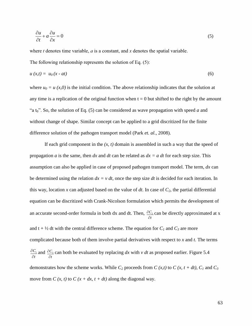
63

0u u

at x

(5)

where t denotes time variable, a is a constant, and x denotes the spatial variable.

The following relationship represents the solution of Eq. (5):

u (x,t) = u0 (x - at) (6)

where u0 = u (x,0) is the initial condition. The above relationship indicates that the solution at

any time is a replication of the original function when t = 0 but shifted to the right by the amount

“a t0”. So, the solution of Eq. (5) can be considered as wave propagation with speed a and

without change of shape. Similar concept can be applied to a grid discritized for the finite

difference solution of the pathogen transport model (Park et. al., 2008).

If each grid component in the (x, t) domain is assembled in such a way that the speed of

propagation a is the same, then dx and dt can be related as dx = a dt for each step size. This

assumption can also be applied in case of proposed pathogen transport model. The term, dx can

be determined using the relation dx = v dt, once the step size dt is decided for each iteration. In

this way, location x can adjusted based on the value of dt. In case of C2, the partial differential

equation can be discritized with Crank-Nicolson formulation which permits the development of

an accurate second-order formula in both dx and dt. Then, 2C

t

can be directly approximated at x

and t + ½ dt with the central difference scheme. The equation for C1 and C3 are more

complicated because both of them involve partial derivatives with respect to x and t. The terms

1C

t

and 3C

t

can both be evaluated by replacing dx with v dt as proposed earlier. Figure 5.4

demonstrates how the scheme works. While C2 proceeds from C (x,t) to C (x, t + dt), C1 and C3

move from C (x, t) to C (x + dx, t + dt) along the diagonal way.

64

When the surface cover is vegetated, an extra equation along with two additional terms

was added to the model which could represent attachment to the vegetation with the rate with k14

and detachment from the vegetation with the rate k41. The system of equations in case of

vegetated surface is as follows:

(7)

(8)

(9)

(10)

5.1 Model parameter identification

For the pathogen transport study, a 40-minute single storm simulation on a laboratory

tilting bed was performed. The input for this simulation included: climate data including date of

the storm, the storm amount, and the storm duration; hillslope profile including shape, area, and

inclination of the hillslope; field operation and crop conditions; soil parameters, etc.

The WEPP simulations provided: (1) effective rainfall intensity; (2) effective saturated

conductivity, which is the same as the infiltration rate when some 95% of the total pore space is

filled with water; (3) average flow depth and average flow rate, which can be derived from the

Chezy coefficient and the peak runoff rate; (4) average soil loss per detachment area; (5) the soil

particle fraction exiting in flow.

1 112 14 1 21 2 41 4

212 1 23 21 2

3 323 2 3

414 1 41 4

( )

( )

( )

d

d

C C fu K K K C K C K C

t x D

CK C K K C

t

C C fu K C K C

t x D

CK C K C

t

65

Figure 5.4 Grid discritized for the finite difference solution (Chow et al., 1988).

Microorganisms and soil particles can be thought of as chemical substances that react with

each other producing the third substance: microorganism-soil particle aggregates for modeling

purposes (Yeghiazarian et al., 2006). The strength of attachment of microorganisms to soil

particles is determined by the chemical characteristics of soils which are highly correlated with

the particle size. For example, the study by McLaughlin (2003) reported that C. parvum oocysts

strongly adsorb to clay particles compared to silt or sand particles. The physical, and hence, the

mathematical representation of inter-particle interactions may be further simplified by

considering that the amount of soil particles participating in “reactions” is either infinite (number

of soil particles on the soil surface), or can be obtained experimentally or from an erosion model

Tim

e t

Δx

Δt

Distance x

i Δx

(i+1) Δx

j Δt

(j+1) Δt

Known value of C

Unknown value of C

66

(suspended sediment). The particle size class distribution of sediment in the suspended sediment

is predicted by the WEPP model. As the microorganism transport model uses WEPP output as its

input, the transport model was coupled with WEPP model externally.

Initial approximation for K12 is obtained from Ling et al. (2003). They came up with an

approximation for partitioning coefficient (Kd) for bacteria with the long centrifuge experiment.

They found Kd to be a function of the clay content in soil as:

Kd = A (CLAY)B (11)

where CLAY = the percentage of clay particles <0.002mm in soil (the relationship was developed

for 2 < CLAY % < 50), A = the slope of the regression in log-log coordinates (10-1.6 0.9

), B = the

intercept of the regression in log-log coordinates (1.98 0.7).

Parameter K23 is the rate of microorganism-soil particle aggregate removal from the soil

surface. Parameters involving free microorganism/aggregate removal from the soil surface are

obtained by analogy with soil erosion processes. Soil erosion mainly occurs via two mechanisms:

a) raindrop impact, and b) erosion caused by flowing water due to the effect of shear stress acting

at the interface between flowing water and the soil surface. The effect of these mechanisms is

additive. Hence, initial approximation for K23 is computed as sum of raindrop erosion and

erosion induced by flow velocity as (d23 P + e23 vS). Here, d23 (=1/D) is detachability coefficient,

P is the rainfall intensity obtained from the erosion model, e23 is the coefficient of micro-

aggregate entrainment by the flow, v is the flow velocity and S is the slope (Yeghiazarian et al.,

2006).

Both vegetation related parameters K14 and K41 were treated as calibration parameters in the

absence of reliable parameter estimate in the literatures.

67

CHAPTER 6: RESULTS AND DISCUSSION

This section provides the details of laboratory experiment and model simulation results. The

model simulated results were compared with the following experimental data sets:

1. Large scale laboratory experiment: Flow and C. parvum recovery from two soil types

(Catlin and Newberry), two rainfall conditions (2.54 and 6.35 cm/hr) and three bed slope

conditions (1.5, 3.0 and 4.5%) for bare and vegetated (Brome grass) conditions

2. Small scale experiment:

(a) Flow, C. parvum and rotavirus recovery from three soil type (Alvin, Catlin and

Darwin), three surface conditions (bare, Brome grass and Fescue) with 2.5% bed slope

subjected 6.35 cm/hr rainfall

(b) Flow and C. parvum recovery from Catlin soil bed with 2.5% slope subjected 6.35

cm/hr rainfall and 3.0% slope subjected to 9.0 cm/hr rainfall intensity for bare and

vegetated (Brome grass) conditions

3. Laboratory experiment on runoff induced erosion: Flow and sediment

6.1 Results from large-scale laboratory experiment

As mentioned earlier, a series of laboratory experiments were conducted by Trask (2002) using

three slopes (1.5, 3.0, and 4.5%), two rainfall intensities (2.54 and 6.35 cm/hr), one vegetation

type (Brome) and two soil types (Catlin and Newberry). C. parvum oocysts were detected in both

surface runoff and near-surface flow for both bare-ground and vegetated conditions for each

slope (1.5, 3.0, and 4.5%) under low rainfall intensity (2.54 cm/hr) conditions following the

initial application of pathogens. For the high intensity rainfall (6.35 cm/hr), C. parvum oocysts

68

were detected in surface runoff from bare-ground and vegetated conditions while near-surface

flow contained detectable oocysts from the vegetated conditions with zero flow from the bare-

ground conditions from all slope conditions.

6.1.1 Runoff volume

As observed by Trask (2002), the volumes of surface runoff obtained from the bare-ground

conditions were consistently higher than those from vegetated conditions. This trend was

observed for all slope conditions, both rainfall intensities and soil types. These findings were

expected because reduced runoff volumes from the VFS were associated with more resistance to

overland flow and longer contact times allowing a higher infiltration of water into the soil

profile. The collected runoff volumes for the 1.5, 3.0, and 4.5% slopes are presented in Table 6.1

for Catlin soil and in Table 6.2 for Newberry soil respectively as reported by Trask (2002).

Table 6.1 Volumes of surface runoff and near-surface flow (in liters) at three different slopes

for 2.54 and 6.35-cm/hr rainfall intensities for Catlin soil.

Collection Type

Volumes in Liters

2.54-cm/hr Rainfall 6.35-cm/hr Rainfall

Slope

1.5%

Slope

3.0%

Slope

4.5%

Slope

1.5%

Slope

3.0%

Slope

4.5%

Bare-ground surface runoff 31.0 39.2 34.4 111.8 109.0 104.7

Vegetative surface runoff 17.5 27.3 24.5 56.5 68.7 76.4

Bare-ground near-surface flow 3.1 1.8 0.6 0.0 0.0 0.0

Vegetative near-surface flow 10.1 8.6 5.2 9.0 13.9 11.5

69

Table 6.2 Volumes of surface runoff and near-surface flow (in liters) at three different slopes

for 2.54 and 6.35-cm/hr rainfall intensities for Newberry soil.

Collection Type

Volumes in Liters

2.54-cm/hr Rainfall 6.35-cm/hr Rainfall

Slope

1.5%

Slope

3.0%

Slope

4.5%

Slope

1.5%

Slope

3.0%

Slope

4.5%

Bare-ground surface runoff 35.2 45.3 50.5 116.6 115.9 118.8

Vegetative surface runoff 23.5 26.5 27.9 60.4 65.6 71.6

Bare-ground near-surface flow 3.8 2.9 3.1 0.0 0.0 0.0

Vegetative near-surface flow 10.8 8.2 4.7 12.1 11.2 9.5

6.1.2 C. parvum oocyst recovery

As reported by Trask (2002), the oocyst recovery rates in surface runoff for both 2.54 and 6.35

cm/hr rainfall intensities for different slopes varied. For light intensity rainfall event (2.54-

cm/hr), there was a greater recovery of oocysts from the 1.5% slope as compared to those from

the 3.0 and 4.5% slopes as shown in Tables 6.3 and 6.4.

Table 6.3 Total percent recovery of applied oocysts for surface and near-surface flow for bare

ground and vegetated condition for Catlin soil.

Surface condition

Recovery in %

2.54-cm/hr Rainfall 6.35-cm/hr Rainfall

Slope

1.5%

Slope

3.0%

Slope

4.5%

Slope

1.5%

Slope

3.0%

Slope

4.5%

Bare-ground surface 13.77 9.53 3.35 2.53 5.32 52.45

Bare-ground near-surface 0.04 0.02 0.00 0.00 0.00 0.00

Vegetated surface 1.65 0.84 0.34 0.80 0.39 20.34

Vegetated near-surface 1.25 0.04 0.01 0.08 0.18 1.62

70

Table 6.4 Total percent recovery of applied oocysts for surface and near-surface flow for bare

ground and vegetated condition for Newberry soil.

Surface condition

Recovery in %

2.54 cm/hr Rainfall 6.35 cm/hr Rainfall

Slope

1.5%

Slope

3.0%

Slope

4.5%

Slope

1.5%

Slope

3.0%

Slope

4.5%

Bare-ground surface 20.08 4.17 9.30 17.16 79.69 98.50

Bare-ground near-surface 0.03 0.01 0.00 0.00 0.00 0.00

Vegetated surface 6.88 0.51 0.64 1.57 2.93 8.27

Vegetated near-surface 0.65 0.03 0.01 0.00 0.10 0.65

6.2 Results from small-scale laboratory experiment

A series of laboratory experiments were conducted at the University of Illinois at Urbana-

Champaign from 2007-2009. The experiments conducted by Koch (2009) included two sets of

slope and intensity conditions (2.5% slope and 6.35 cm/hr intensity along with 3.0% slope and

9.0 cm/hr rainfall intensity), Catlin soil bed with and without vegetation (Brome grass).

Experiments conducted by Davidson (2010) used three types of soil beds (a moderately drained

Catlin silt-loam, Alvin fine sandy-loam, Darwin silty-clay soil) set at 2.5% slope under simulated

rainfall intensity 6.35 cm/hr with three surface conditions: bare, Brome grass and Fescue.

6.2.1 Runoff Volume and oocyst recovery

Table 6.5 summarizes the runoff volume and oocysts recovery from a Catlin soil bed with

and without vegetation under different slopes (2.5 and 3.0%) and rainfall intensities (6.35 and 9.0

cm/hr) as reported by Koch (2009).

71

Table 6.5 Runoff volumes and oocysts recovery from a small-scale Catlin soil bed.

Sampling

Location

Surface

Condition

Bed

Slope

Rainfall

Intensity Total Runoff

(mL)

Oocyst

recovery

(%) % cm/hr

Surface Bare 2.5 6.5 1847.0 14.6

Surface Vegetated 2.5 6.5 1633.0 7.1

Near-Surface Bare 2.5 6.5 0.0 0.0

Near-Surface Vegetated 2.5 6.5 9.5 0.0

Surface Bare 3.0 9.0 2645.0 2.45

Surface Vegetated 3.0 9.0 1950.0 1.47

Near-Surface Bare 3.0 9.0 0.0 0.0

Near-Surface Vegetated 3.0 9.0 43.0 0.0

Similarly, Table 6.6 and 6.7 summarize the runoff volume and pathogen recovery from a

three types of soil bed with and without vegetation with 2.5% slope and 65 mm/hr rainfall

intensity for three different cover conditions: bare, Brome grass and Fescue, in surface flow as

reported by Davidson (2010).

Table 6.6 Runoff volumes and C. parvum recovery from a small-scale different soil beds.

Pathogen Type Surface Condition Soil type Total Runoff

(mL)

Pathogen

recovery

(%)

C. parvum Bare Catlin 4384.0 33.38

C. parvum Vegetated (Brome) Catlin 2387.0 14.91

C. parvum Vegetated (Fescue) Catlin 284.0 22.07

C. parvum Bare Darwin 3189.0 38.58

C. parvum Vegetated (Brome) Darwin 2711.0 8.81

C. parvum Vegetated (Fescue) Darwin 467.0 0.00

C. parvum Bare Alvin 3140.0 1.17

C. parvum Vegetated (Brome) Alvin 2139.0 1.10

C. parvum Vegetated (Fescue) Alvin 1301.0 0.06

72

Table 6.7 Runoff volumes and rotavirus recovery from a small-scale different soil beds.

Pathogen Type Surface Condition Soil type Total Runoff

(mL)

Pathogen

recovery

(%)

Rotavirus Bare Catlin 4384.0 34.92

Rotavirus Vegetated (Brome) Catlin 2387.0 9.87

Rotavirus Vegetated (Fescue) Catlin 2894.0 14.23

Rotavirus Bare Darwin 3189.0 26.56

Rotavirus Vegetated (Brome) Darwin 2711.0 16.91

Rotavirus Vegetated (Fescue) Darwin 467.0 0.08

Rotavirus Bare Alvin 3140.0 8.28

Rotavirus Vegetated (Brome) Alvin 2139.0 0.67

Rotavirus Vegetated (Fescue) Alvin 1301.0 1.83

6.3 Modeling result

The simulations were carried out a system identical to the large-scale experimental setup

described by Trask (2002). For WEPP model simulation, many input parameters were obtained

from the experimental setup such as soil plot length of 3.6 m, rainfall intensity of 2.54 and 6.35

mm/hr applied for 40 minutes and two different soil types (Catlin and Newberry). Similarly, the

simulations were carried out two smaller systems identical to the experimental setup described

Davidson (2010) and by Koch (2009). The model results are compared with experimental data.

6.3.1 Comparison of simulated runoff with the observations from large scale experiment

For bare ground simulations, initial saturation level (antecedent moisture content) for the soil and

hydraulic conductivity were used as the calibration parameters. The parameter was calibrated in

such a way that Nash-Sutcliffe efficiency index (EI) and coefficient of determination (R2)

between observed and simulated runoff rate were maximized. The Nash–Sutcliffe efficiency

73

index (EI) has been widely used to assess the predictive power of hydrological models and is

defined as:

(12)

where is observed discharge, is modeled discharge,

is observed discharge at time t,

and Qo is average of observed discharge (Nash and Sutcliffe, 1970). The values for EI can range

from −∞ to 1. An EI value of 1 corresponds to a perfect match of modeled discharge to the

observed data, whereas an EI value of 0 indicates that the model predictions are as accurate as

the mean of the observed data. EI value of less than zero indicates that the observed mean is a

better predictor than the model. In other words, when the residual variance (described by the

nominator in the expression above) is larger than the data variance (described by the

denominator), EI value will be less than zero. Since simulated discharge hydrograph had more

points compared to observation, the simulated discharge value corresponding to observation at

that particular time stamp was used to compute EI and R2. In the absence of sediment data,

WEPP model was calibrated using runoff only.

Comparison of simulated WEPP model result with observations is presented in Figures

6.1-6.20 below. Although total runoff volume and oocyst recovery data was available, runoff

hydrograph and oocysts break-through curve data was not available for low intensity rainfall

experiments (2.54 cm/hr) with Catlin soil bed. So, WEPP simulations were carried out for Catlin

soil beds with three different slope conditions subjected to high intensity of simulated rainfall

(6.35 cm/hr). Figures 6.1, 6.2 and 6.3 show the comparison of the observation with WEPP

simulation result for surface runoff for bare ground condition, 6.35 cm/hr rainfall applied for 40

74

minutes at 1.5, 3 and 4.5% slope conditions, respectively for Catlin soil. In all three cases, WEPP

model results were in good agreement with the observations as shown below which is also

demonstrated by statistical analysis. Computed R2 values for 1.5, 3.0 and 4.5% slope conditions

were 0.81, 0.64 and 0.83, respectively. Similarly, computed EI value between observed and

simulated flow were for 1.5, 3.0 and 4.5% slope condition were 0.26, 0.42 and 0.66, respectively.

Figure 6.1 WEPP simulation result for surface runoff for bare ground condition, 6.35 cm/hr

rainfall applied for 40 minutes at 1.5% slope conditions for Catlin soil.

0

5

10

15

20

25

30

35

40

45

50

55

60

0 5 10 15 20 25 30 35 40 45 50 55 60 65

Dis

ch

arg

e (

cm

3/s

)

Time (minute)

Discharge (cm3/s) Observed

Simulated

75

Figure 6.2 WEPP simulation result for surface runoff for bare ground condition, 6.35 cm/hr

rainfall applied for 40 minutes at 3.0% slope conditions for Catlin soil.

Figure 6.3 WEPP simulation result for surface runoff for bare ground condition, 6.35 cm/hr

rainfall applied for 40 minutes at 4.5% slope conditions for Catlin soil.

Figures 6.4, 6.5 and 6.6 show the comparison of the observation with WEPP simulation

result for surface runoff for bare ground condition, 2.54 cm/hr rainfall applied for 40 minutes at

0

5

10

15

20

25

30

35

40

45

50

55

60

65

0 5 10 15 20 25 30 35 40 45 50 55

Dis

ch

arg

e (

cm

3/s

)

Time (minute)

Observed

Simulated

0

5

10

15

20

25

30

35

40

45

50

55

0 5 10 15 20 25 30 35 40 45 50 55

Dis

ch

arg

e (

cm

3/s

)

Time (minute)

Observed

Simulated

76

1.5, 3 and 4.5% slope conditions, respectively for Newberry soil. As in case of Catlin soil, initial

saturation level (antecedent moisture content) and hydraulic conductivity were the calibration

parameters for WEPP simulation for Newberry soil bare ground condition. It was noted that

antecedent moisture content affected when runoff started while hydraulic conductivity governed

the peak runoff rate and total runoff volume. In all three cases, WEPP model results were in

good agreement with the observations as shown below which is also substantiated by statistical

analysis of observed and simulated runoff. Computed R2 values for 1.5, 3.0 and 4.5% slope

conditions were 0.63, 0.84 and 0.46, respectively. Similarly, computed EI values for 1.5, 3.0 and

4.5% slope condition were 0.25, 0.28 and -1.35, respectively. Negative value of EI indicates that

the residual variance is larger than the data variance.

Figure 6.4 WEPP simulation results for surface runoff for bare ground condition, 2.54 cm/hr

rainfall applied for 40 minutes at 1.5% slope conditions for Newberry soil.

0

5

10

15

20

0 5 10 15 20 25 30 35 40 45 50 55 60

Dis

ch

arg

e (

cm

3/s

)

Time (minute)

ObservedSimulated

77

Figure 6.5 WEPP simulation result for surface runoff for bare ground condition, 2.54 cm/hr

rainfall applied for 40 minutes at 3.0% slope conditions for Newberry soil.

Figure 6.6 WEPP simulation result for surface runoff for bare ground condition, 2.54 cm/hr

rainfall applied for 40 minutes at 4.5% slope conditions for Newberry soil.

0

5

10

15

20

0 5 10 15 20 25 30 35 40 45 50 55 60

Dis

ch

arg

e (

cm

3/s

)

Time (minute)

Observed

Simulated

0

5

10

15

20

0 5 10 15 20 25 30 35 40 45 50 55

Dis

ch

arg

e (

cm

3/s

)

Time (minute)

Observed

Simulated

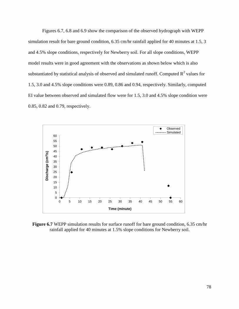
78

Figures 6.7, 6.8 and 6.9 show the comparison of the observed hydrograph with WEPP

simulation result for bare ground condition, 6.35 cm/hr rainfall applied for 40 minutes at 1.5, 3

and 4.5% slope conditions, respectively for Newberry soil. For all slope conditions, WEPP

model results were in good agreement with the observations as shown below which is also

substantiated by statistical analysis of observed and simulated runoff. Computed R2 values for

1.5, 3.0 and 4.5% slope conditions were 0.89, 0.86 and 0.94, respectively. Similarly, computed

EI value between observed and simulated flow were for 1.5, 3.0 and 4.5% slope condition were

0.85, 0.82 and 0.79, respectively.

Figure 6.7 WEPP simulation results for surface runoff for bare ground condition, 6.35 cm/hr

rainfall applied for 40 minutes at 1.5% slope conditions for Newberry soil.

0

5

10

15

20

25

30

35

40

45

50

55

60

0 5 10 15 20 25 30 35 40 45 50 55 60

Dis

ch

arg

e (

cm

3/s

)

Time (minute)

Observed

Simulated

79

Figure 6.8 WEPP simulation results for surface runoff for bare ground condition, 6.35 cm/hr

rainfall applied for 40 minutes at 3.0% slope conditions for Newberry soil.

Figure 6.9 WEPP simulation results for surface runoff for bare ground condition, 6.35 cm/hr

rainfall applied for 40 minutes at 4.5% slope conditions for Newberry soil.

0

5

10

15

20

25

30

35

40

45

50

55

60

0 5 10 15 20 25 30 35 40 45 50 55 60

Dis

ch

arg

e (

cm

3/s

)

Time (minute)

Observed

Simulated

0

5

10

15

20

25

30

35

40

45

50

55

0 5 10 15 20 25 30 35 40 45 50 55

Dis

ch

arg

e (

cm

3/s

)

Time (minute)

ObservedSimulated

80

In case of vegetated condition, soil parameters (initial saturation level and hydraulic

conductivity) along with vegetation parameters (canopy, interrill and rill cover, roughness after

tillage) were WEPP model calibration parameters. Comparison of observed hydrograph with

WEPP simulated result for vegetated condition, 6.35 cm/hr rainfall applied for 40 minutes at 1.5,

3.0 and 4.5% slope conditions for Catlin soil are presented in Figures 6.10 - 6.12. Since the

moisture holding capacity of bare ground and vegetated surface is different, the soil parameters

were calibrated separately for those two conditions. As the moisture condition in the laboratory

varied for each set of run, separate parameters were calibrated for different rainfall intensities

and slope conditions. WEPP model could replicate observed runoff pattern fairy well for all three

slope conditions results as demonstrated statistical analysis. Computed R2 values for 1.5, 3.0 and

4.5% slope conditions were 0.60, 0.71 and 0.57, respectively. Similarly, computed EI value

between observed and simulated flow were for 1.5, 3.0 and 4.5% slope condition were 0.51, 0.67

and -0.05, respectively. Negative value of EI for 4.5% slope condition indicates that the residual

variance is larger than the (observed) data variance.

Figure 6.10 WEPP simulation results for surface runoff for vegetated condition, 6.35 cm/hr

rainfall applied for 40 minutes at 1.5% slope conditions for Catlin soil.

0

5

10

15

20

25

30

35

40

45

0 5 10 15 20 25 30 35 40 45 50 55 60 65 70 75 80

Dis

ch

arg

e (

cm

3/s

)

Time (minute)

Observed

Simulated

81

Figure 6.11 WEPP simulation results for surface runoff for vegetated condition, 6.35 cm/hr

rainfall applied for 40 minutes at 3.0% slope conditions for Catlin soil.

Figure 6.12 WEPP simulation results for surface runoff for vegetated condition, 6.35 cm/hr

rainfall applied for 40 minutes at 4.5% slope conditions for Catlin soil.

For Newberry soil with vegetated surface, both soil parameters (initial saturation level

and hydraulic conductivity) along with the vegetation parameters (canopy, interrill and rill cover,

0

5

10

15

20

25

30

35

40

45

50

0 5 10 15 20 25 30 35 40 45 50 55 60 65 70 75 80

Dis

ch

arg

e (

cm

3/s

)

Time (minute)

Observed

Simulated

0

5

10

15

20

25

30

35

40

45

50

0 10 20 30 40 50 60

Dis

ch

arg

e (

cm

3/s

)

Time (minute)

Observed

Simulated

82

roughness after tillage) were used as calibration parameters for WEPP model to simulate surface

runoff. Comparisons of observed hydrograph with WEPP simulation results for vegetated

condition, 2.54 cm/hr rainfall applied for 40 minutes at 1.5, 3 and 4.5% slope conditions

respectively for Newberry soil are presented in Figures 6.13, 6.14 and 6.15. Compared to earlier

simulation results, WEPP model could not replicate observed hydrograph fairy well in these

three conditions. Computed R2 values (for observed and simulated runoff values) for 1.5, 3.0 and

4.5% slope conditions were 0.39, 0.79 and 0.58, respectively. Similarly, computed EI value

between observed and simulated flow were for 1.5, 3.0 and 4.5% slope condition were -0.03,

0.20 and -0.11, respectively.

Figure 6.13 WEPP simulation results for surface runoff for vegetated condition, 2.54 cm/hr

rainfall applied for 40 minutes at 1.5% slope conditions for Newberry soil.

0

5

10

0 5 10 15 20 25 30 35 40 45 50 55 60

Dis

ch

arg

e (

cm

3/s

)

Time (minute)

Observed

Simulated

83

Figure 6.14 WEPP simulation results for surface runoff for vegetated condition, 2.54 cm/hr

rainfall applied for 40 minutes at 3.0% slope conditions for Newberry soil.

Figure 6.15 WEPP simulation results for surface runoff for vegetated condition, 2.54 cm/hr

rainfall applied for 40 minutes at 4.5% slope conditions for Newberry soil.

Comparisons of observed hydrograph with WEPP simulation results for vegetated

condition, 6.35 cm/hr rainfall applied for 40 minutes at 1.5, 3 and 4.5% slope conditions

respectively for Newberry soil are presented in Figures 6.16 - 6.18. In case of 1.5% slope

0

5

10

0 5 10 15 20 25 30 35 40 45 50 55 60

Dis

ch

arg

e (

cm

3/s

)

Time (minute)

Observed

Simulated

0

5

10

0 5 10 15 20 25 30 35 40 45 50 55

Dis

ch

arg

e (

cm

3/s

)

Time (minute)

Observed

Simulated

84

condition, multiple peaks were detected in observed hydrograph. Those multiple peaks could not

be replicated by WEPP simulation result which is evident by low R2 (0.18) and negative EI value

(-0.23). In case of 3.0 and 4.5% bed slope conditions, WEPP model could replicate the pattern of

observed hydrograph as demonstrated by statistical analysis. Computed R2 values (for observed

and simulated runoff values) for 3.0 and 4.5% slope conditions were 0.74 and 0.75, respectively.

Similarly, computed EI values for 3.0 and 4.5% slope conditions were 0.66 and 0.74,

respectively.

Figure 6.16 WEPP simulation results for surface runoff for vegetated condition, 6.35 cm/hr

rainfall applied for 40 minutes at 1.5% slope conditions for Newberry soil.

0

5

10

15

20

25

30

35

40

45

50

0 5 10 15 20 25 30 35 40 45 50

Dis

ch

arg

e (

cm

3/s

)

Time (minute)

ObservedSimulated

85

Figure 6.17 WEPP simulation results for surface runoff for vegetated condition, 6.35 cm/hr

rainfall applied for 40 minutes at 3.0% slope conditions for Newberry soil.

Figure 6.18 WEPP simulation results for surface runoff for vegetated condition, 6.35 cm/hr

rainfall applied for 40 minutes at 4.5% slope conditions for Newberry soil.

0

5

10

15

20

25

30

35

40

45

50

0 5 10 15 20 25 30 35 40 45 50 55 60 65 70 75

Dis

ch

arg

e (

cm

3/s

)

Time (minute)

Observed

Simulated

0

5

10

15

20

25

30

35

40

45

0 5 10 15 20 25 30 35 40 45 50 55 60 65 70 75

Dis

ch

arg

e (

cm

3/s

)

Time (minute)

Observed

Simulated

86

Figures 6.19 and 6.20 show the comparison of simulated results from WEPP for total runoff

volume with observation for all surface cover, slope and rainfall conditions. In case of Catlin

soil, the results obtained from WEPP simulation for total runoff volume result were similar to

those from laboratory experiment as shown in Figure 6.19. Similarly, observed and simulated

total runoff volume in different rainfall, slope and cover condition for Newberry soil also showed

a good agreement as presented in Figure 6.20. These results indicate that WEPP model can

predict surface runoff rate and total volume fairly well in case of small scale laboratory

experiments.

Figure 6.19 Comparison of WEPP simulation results with observations for surface runoff

volume for different slopes, rainfall and surface cover conditions for Catlin soil.

R² = 0.9735

0

20

40

60

80

100

120

140

0 20 40 60 80 100 120 140

Sim

ula

ted

vo

lum

e (

L)

Observed volume (L)

Linear (1:1)

87

Figure 6.20 Comparison of WEPP simulation results with observations for surface runoff

volume for different slopes, rainfall and surface cover conditions for Newberry soil.

6.3.2 Comparison of simulated runoff with the observations from small scale experiments

WEPP simulations were carried out for Alvin, Catlin and Darwin soil beds with 2.5%

slope with three different cover conditions: bare, Brome and Fescue grasses replicating the

experimental conditions of Davidson (2010). The soil beds were subjected a simulated rainfall

intensity of 6.35 cm/hr applied for 20 minutes. These soil beds were 0.61 m (2 ft) long, 0.305 m

(1 ft) wide and 0.015 m (0.5 ft) thick. Figures 6.21, 6.22 and 6.23 show the comparison of the

observation with WEPP simulation result for surface runoff for bare ground and two vegetated

conditions for Alvin soil. In all three cases, WEPP model produced reasonable results as

compared with the observations as shown below, which is also demonstrated by statistical

analysis. Computed R2 values for bare, Brome and Fescue cover conditions were 0.62, 0.37 and

0.48, respectively. Similarly, computed EI value between observed and simulated flow for bare,

Brome and Fescue cover conditions were 0.56, -0.63 and -0.12, respectively.

R² = 0.97

0

20

40

60

80

100

120

140

0 20 40 60 80 100 120 140

Sim

ula

ted

vo

lum

e (

L)

Observed volume (L)

Linear (1:1)

88

Figure 6.21 WEPP simulation results for surface runoff for bare Alvin soil bed subjected to 6.35

cm/hr rainfall applied for 20 minutes at 2.5% slope.

Figure 6.22 WEPP simulation results for surface runoff for Alvin soil bed with Brome grass

cover subjected to 6.35 cm/hr rainfall applied for 20 minutes at 2.5% slope.

0

50

100

150

200

250

0 5 10 15 20 25 30

Ru

no

ff r

ate

(m

l/m

in)

Time (min)

ObservedSimulated

0

20

40

60

80

100

120

140

0 5 10 15 20 25 30

Ru

no

ff r

ate

(m

l/m

in)

Time (min)

ObservedSimulated

89

Figure 6.23 WEPP simulation results for surface runoff for Alvin soil bed with Fescue cover

subjected to 6.35 cm/hr rainfall applied for 20 minutes at 2.5% slope.

Figures 6.24, 6.25 and 6.26 show the comparison of the experimental data with WEPP

simulation result for surface runoff for bare ground and two vegetated conditions for Catlin soil.

WEPP model results were in a good agreement with the experimental data as shown below

which is also demonstrated by statistical analysis. Computed R2 values for bare, Brome and

Fescue cover conditions were 0.65, 0.41 and 0.81, respectively. Similarly, computed EI value

between observed and simulated flow for bare, Brome and Fescue cover conditions were 0.93,

0.86 and 0.65, respectively.

0

10

20

30

40

50

60

70

80

90

0.0 5.0 10.0 15.0 20.0 25.0

Ru

no

ff r

ate

(m

l/m

in)

Time (min)

Observed

Simulated

90

Figure 6.24 WEPP simulation results for surface runoff for bare Catlin soil bed subjected to 6.35

cm/hr rainfall applied for 20 minutes at 2.5% slope.

Figure 6.25 WEPP simulation results for surface runoff for Catlin soil bed with Brome grass

vegetation subjected to 6.35 cm/hr rainfall applied for 20 minutes at 2.5% slope.

0

50

100

150

200

250

300

0.0 5.0 10.0 15.0 20.0 25.0 30.0

Ru

no

ff r

ate

(m

l/m

in)

Time (min)

Observed

Simulated

0

20

40

60

80

100

120

140

160

0.0 5.0 10.0 15.0 20.0 25.0 30.0

Ru

no

ff r

ate

(m

l/m

in)

Time (min)

Observed

Simulated

91

Figure 6.26 WEPP simulation results for surface runoff for Catlin soil bed with Fescue

vegetation subjected to 6.35 cm/hr rainfall applied for 20 minutes at 2.5% slope.

The comparison of the experimental data with WEPP simulation result for surface runoff

for bare ground and two vegetated conditions for Darwin soil is presented in Figures 6.27, 6.28

and 6.29 below. WEPP model results showed a good agreement with the experimental data

which is also demonstrated by statistical analysis. Computed R2 values for bare, Brome and

Fescue cover conditions were 0.78, 0.83 and 0.72, respectively. Similarly, computed EI value

between observed and simulated flow for bare, Brome and Fescue cover conditions were 0.64,

0.71 and -4.27, respectively. Observed surface runoff rate for Darwin soil bed with Fescue

vegetation was much less compared to runoff data for Brome grass cover condition for the

similar condition. The difference in factors like root zone depth, surface cover and leaf area

index between Brome grass and Fescue may be attributed to the decrease in surface runoff rate.

This might have resulted the over estimation of WEPP simulation result compared to

experimental data for this particular condition as observed in Figure 6.29.

0

20

40

60

80

100

120

140

160

180

200

0.0 5.0 10.0 15.0 20.0 25.0

Ru

no

ff r

ate

(m

l/m

in)

Time (min)

ObservedSimulated

92

Figure 6.27 WEPP simulation results for surface runoff for bare Darwin soil bed subjected to

6.35 cm/hr rainfall applied for 20 minutes at 2.5% slope.

Figure 6.28 WEPP simulation results for surface runoff for Darwin soil bed with Brome grass

vegetation subjected to 6.35 cm/hr rainfall applied for 20 minutes at 2.5% slope.

0

50

100

150

200

250

0.0 5.0 10.0 15.0 20.0 25.0 30.0

Ru

no

ff r

ate

(m

l/m

in)

Time (min)

Observed

Simulated

0

20

40

60

80

100

120

140

160

180

200

0.0 5.0 10.0 15.0 20.0 25.0 30.0

Ru

no

ff r

ate

(m

l/m

in)

Time (min)

Observed

Simulated

93

Figure 6.29 WEPP simulation results for surface runoff for Darwin soil bed with Fescue

vegetation subjected to 6.35 cm/hr rainfall applied for 20 minutes at 2.5% slope.

Koch (2009) carried out laboratory experiments using small scale bare and vegetated

Catlin soil beds with 2.5% slope subjected to 6.35 cm/hr (2.5 in/hr) rainfall applied for 10

minutes. Similarly, he also carried out another set of experiments using small scale bare and

vegetated Catlin soil beds with 3.0% slope subjected to 8.9 cm/hr (3.5 cm/hr) rainfall applied for

10 minutes. WEPP simulations were carried out to replicate these four conditions. Figures 6.30

and 6.31 show the comparison of the observation with WEPP simulation result for surface runoff

for bare ground and vegetated conditions. In both cases, WEPP model produced reasonable

results as compared with the observations as shown below which is also demonstrated by

statistical analysis. Computed R2 values for bare, Brome grass cover conditions were 0.75 and

0.82, respectively. Similarly, computed EI value between observed and simulated flow for bare

and Brome grass cover conditions were 0.42 and 0.66, respectively.

0

10

20

30

40

50

60

70

80

90

100

0.0 5.0 10.0 15.0 20.0 25.0

Ru

no

ff r

ate

(m

l/m

in)

Time (min)

Observed

Simulated

94

Figure 6.30 WEPP simulation results for surface runoff for bare Catlin soil bed with 2.5% slope

subjected to 6.35 cm/hr rainfall applied for 10 minutes.

Figure 6.31WEPP simulation results for surface runoff for Catlin soil bed with at 2.5% slope

and Brome grass vegetation subjected to 6.35 cm/hr rainfall applied for 10 minutes.

Figures 6.32 and 6.33 show the comparison of the observation with WEPP simulation

result for surface runoff for bare ground and vegetated conditions for 3.0% Catlin soil beds. In

both cases, WEPP model produced reasonable results as compared with the observations as

shown below which is also demonstrated by statistical analysis. Computed R2 values for bare,

Brome grass cover conditions were 0.66 and 0.74, respectively. Similarly, computed EI value

0

50

100

150

200

250

0 2 4 6 8 10 12 14 16

Ru

no

ff r

ate

(m

l/m

in)

Time (min)

Observed

Simulated

0

50

100

150

200

250

0 5 10 15 20 25

Ru

no

ff r

ate

(m

l/m

in)

Time (min)

Observed

Simulated

95

between observed and simulated flow for bare and Brome grass cover conditions were 0.34 and

0.41, respectively.

Figure 6.32 WEPP simulation results for surface runoff for bare Catlin soil bed with 3.0% slope

subjected to 9.0 cm/hr rainfall applied for 10 minutes.

Figure 6.33 WEPP simulation results for surface runoff for Catlin soil bed with 3.0% slope and

Brome grass cover subjected to 9.0 cm/hr rainfall applied for 10 minutes.

0

50

100

150

200

250

300

0 2 4 6 8 10 12 14 16

Ru

no

ff r

ate

(m

l/m

in)

Time (min)

Observed

Simulated

0

50

100

150

200

250

300

0.0 2.0 4.0 6.0 8.0 10.0 12.0 14.0 16.0 18.0

Ru

no

ff r

ate

(m

l/m

in)

Time (min)

Observed

Simulated

96

Figure 6.34 shows the comparison of simulated results from WEPP for total runoff volume with

experimental result from small scale experiments for all surface cover, slope and rainfall

conditions. The comparison graph indicates that that WEPP model can predict surface runoff rate

and total volume fairly well in case of small scale laboratory experiments (R2 = 0.96).

Figure 6.34 Comparison of WEPP simulation results with observations for surface runoff

volume for different slopes, rainfall and surface cover conditions for Alvin, Catlin and Darwin

soils.

6.3.3 Oocyst transport model simulation with large scale experiment data

After calibrating WEPP model successfully, the output from simulated WEPP model was used to

drive oocysts transport model. WEPP model simulations provided input parameters: bed slope,

rainfall intensity, flow velocity, flow depth, saturated hydraulic conductivity and soil loss for

oocysts transport model. During calibration process, break-through curve from the oocysts

R² = 0.9626

0

500

1000

1500

2000

2500

3000

3500

4000

4500

5000

0 1000 2000 3000 4000 5000

Sim

ula

ted

vo

lum

e (

mL)

Observed volume (mL)

Linear (1:1)

97

transport model was compared with the laboratory experiments to estimate different attachment

factors K12, K23, K21.

Figures 6.35, 6.36 and 6.37 show the comparison of break-through curve obtained from

oocysts transport model with experimental data for 1.5, 3.0 and 4.50% slope condition with 6.35

cm/hr rainfall for Catlin soil. In case of 1.5% slope, the model could replicate observed oocysts

pattern fairly well (R2 = 0.88).

Figure 6.35 Comparison of oocyst transport simulation result with observations for bare ground

condition, 6.35 cm/hr rainfall applied for 40 minutes at 1.5% slope for Catlin soil.

For 3.0 and 4.5% slope conditions, the model could reproduce the first oocysts peak

observed during the experiment fairy well but recovery pattern was different from the

observations. As seen in Figure 6.36, experimental data showed a small jump in oocyst recovery

after 30 minutes and the model simulation could not match that jump. Similarly, second peak

was observed around 40 minutes in case of 4.5% slope condition which could not be matched by

simulated model results. Even though the simulated results could match the very first peak

0

0.2

0.4

0.6

0.8

1

1.2

1.4

1.6

1.8

0 10 20 30 40 50 60 70

Oo

cys

ts r

ec

ove

ry %

Time (minute)

Observed

Simulated

98

observed during experiments in most cases, the model could not reproduce multiple peaks

obtained from experimental results and under-predicted total oocysts recovery in few similar

cases. Computed R2 values (for observed and simulated oocysts break-through curve values) for

3.0 and 4.5% slope conditions were 0.48 and 0.11, respectively.

Figure 6.36 Comparison of oocyst transport simulation result with observations for bare ground

condition, 6.35 cm/hr rainfall applied for 40 minutes at 3.0% slope for Catlin soil.

0

0.2

0.4

0.6

0.8

1

1.2

0 10 20 30 40 50 60 70

Oo

cys

ts r

ec

ove

ry %

Time (minute)

Observed

Simulated

99

Figure 6.37 Comparison of oocyst transport simulation result with observations for bare ground

condition, 6.35 cm/hr rainfall applied for 40 minutes at 4.5% slope for Catlin soil.

Figures 6.38 – 6.40 show the comparison of break-through curve obtained from oocysts

transport model with experimental data for 1.5, 3.0 and 4.5% slope condition with 2.54 cm/hr

rainfall for Newberry soil with no cover. The model simulation results are pretty consistent with

experiment data for these singled peak observations as evident by high R2 values (0.64, 0.87 and

0.65 for 1.5, 3.0 and 4.5% bed slope conditions, respectively).

0

2

4

6

8

10

12

14

16

18

20

0 10 20 30 40 50 60 70

% R

ec

ove

ry o

f A

pp

lie

d O

oc

ys

ts

Time (min)

Observed

Simulated

100

Figure 6.38 Oocyst transport simulation result for surface runoff for bare ground condition, 2.54

cm/hr rainfall applied for 40 minutes at 1.5% slope for Newberry soil.

Figure 6.39 Oocyst transport simulation result for surface runoff for bare ground condition, 2.54

cm/hr rainfall applied for 40 minutes at 3.0% slope for Newberry soil.

0.0

2.0

4.0

6.0

8.0

10.0

12.0

0 10 20 30 40 50 60 70

Oo

cys

ts r

ec

ove

ry (

%)

Time (min)

Observed

Simlated

0.0

0.2

0.4

0.6

0.8

1.0

1.2

1.4

1.6

1.8

2.0

0 10 20 30 40 50 60 70

Oo

cys

ts r

ec

ove

ry (

%)

Time (min)

Observed

Simlated

101

Figure 6.40 Oocyst transport simulation result for surface runoff for bare ground condition, 2.54

cm/hr rainfall applied for 40 minutes at 4.5% slope for Newberry soil.

Figures 6.41, 6.42 and 6.43 show the comparison of break-through curve obtained from

oocysts transport model with experimental data for 1.5, 3.0 and 4.5% slope condition with 6.35

cm/hr rainfall for Newberry soil with no cover. For all three cases, the model could reproduce the

first oocysts peak observed during the experiment fairy well but could not capture the second

peak in the observed data. So, the model simulation results were not consistent with experiment

data for these multiple peak observations. Computed R2 values (for observed and simulated

oocysts break-through curve values) for 1.5, 3.0 and 4.5% slope conditions were 0.68, 0.01 and

0.49, respectively.

0.0

0.5

1.0

1.5

2.0

2.5

3.0

3.5

0 10 20 30 40 50 60 70

Oo

cys

ts r

eco

ve

ry (

%)

Time (min)

Observed

Simlated

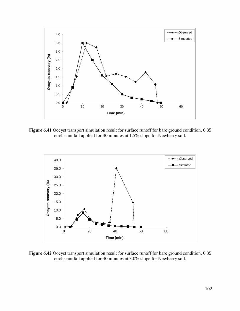
102

Figure 6.41 Oocyst transport simulation result for surface runoff for bare ground condition, 6.35

cm/hr rainfall applied for 40 minutes at 1.5% slope for Newberry soil.

Figure 6.42 Oocyst transport simulation result for surface runoff for bare ground condition, 6.35

cm/hr rainfall applied for 40 minutes at 3.0% slope for Newberry soil.

0.0

0.5

1.0

1.5

2.0

2.5

3.0

3.5

4.0

0 10 20 30 40 50 60

Oo

cys

ts r

ec

ove

ry (

%)

Time (min)

Observed

Simulated

0.0

5.0

10.0

15.0

20.0

25.0

30.0

35.0

40.0

0 20 40 60 80

Oo

cys

ts r

ec

ove

ry (

%)

Time (min)

Observed

Simlated

103

Figure 6.43 Oocyst transport simulation result for surface runoff for bare ground condition, 6.35

cm/hr rainfall applied for 40 minutes at 4.5% slope for Newberry soil.

Figures 6.44, 6.45 and 6.46 show the comparison of break-through curve obtained from

oocysts transport model with experimental data for 1.5, 3.0 and 4.5% slope condition with 6.35

cm/hr rainfall for Catlin soil with vegetation. In case of 1.5% slope, the model could replicate

single-peaked break-through curve fairly well while the model could not capture second peak in

break-through curve in observed data in case of 3 and 4.5 % slope conditions. Computed R2

values (for observed and simulated oocysts break-through curve values) for 1.5, 3.0 and 4.5%

slope conditions were 0.82, 0.60 and 0.41, respectively.

0.0

5.0

10.0

15.0

20.0

25.0

30.0

35.0

40.0

0 10 20 30 40 50 60 70

Oo

cys

ts r

ec

ove

ry (

%)

Time (min)

Observed

Simulated

104

Figure 6.44 Comparison of oocyst transport simulation result with observations for vegetated

Catlin soil bed with 1.5% slope subjected to 6.35 cm/hr rainfall for 40 minutes.

Figure 6.45 Comparison of oocyst transport simulation result with observations for vegetated

Catlin soil bed with 3% slope subjected to 6.35 cm/hr rainfall for 40 minutes.

0

0.05

0.1

0.15

0.2

0.25

0.3

0 10 20 30 40 50 60 70 80

% R

eco

very

of

Ap

plied

Oo

cysts

Time (minute)

Observed

Simulated

0

0.02

0.04

0.06

0.08

0.1

0.12

0 10 20 30 40 50 60 70

% R

ec

ove

ry o

f A

pp

lie

d O

oc

ys

ts

Time (minute)

Observed

Simulated

105

Figure 6.46 Comparison of oocyst transport simulation result with observations for vegetated

Catlin soil bed with 4.5% slope subjected to 6.35 cm/hr rainfall for 40 minutes.

Figures 6.47 – 6.49 show the comparison of break-through curve obtained from oocysts

transport model with experimental data for 1.5, 3.0 and 4.5% slope condition with 2.54 cm/hr

rainfall for Newberry soil with vegetation. The model simulation results are pretty consistent

with experiment data for these singled peak observations as shown in Figures 6.47, 6.48 and 6.4.

Computed R2 values (for observed and simulated oocysts break-through curve values) for 1.5,

3.0 and 4.5% slope conditions were 0.63, 0.90 and 0.50, respectively.

0

1

2

3

4

5

6

7

0 10 20 30 40 50 60

% R

ec

ove

ry o

f A

pp

lie

d O

oc

ys

ts

Time (minute)

Observed

Simulated

106

Figure 6.47 Oocysts transport simulation result for surface runoff for vegetated condition, 2.54

cm/hr rainfall applied for 40 minutes at 1.5% slope for Newberry soil.

Figure 6.48 Oocyst transport simulation result for surface runoff for vegetated condition, 2.54

cm/hr rainfall applied for 40 minutes at 3.0% slope for Newberry soil.

0.00

0.05

0.10

0.15

0.20

0.25

0 10 20 30 40 50 60 70

Oo

cysts

reco

very

(%

)

Time (min)

Observed

Simlated

0.000

0.001

0.002

0.003

0.004

0.005

0.006

0 20 40 60 80

Oo

cysts

reco

very

(%

)

Time (min)

Observed

Simlated

107

Figure 6.49 Oocyst transport simulation result for surface runoff for vegetated condition, 2.54

cm/hr rainfall applied for 40 minutes at 4.5% slope for Newberry soil.

Figures 6.50, 6.51 and 6.52 show the comparison of break-through curve obtained from

oocysts transport model with the experimental data for 1.5, 3.0 and 4.5% slope condition with

6.35 cm/hr rainfall for Newberry soil with vegetation. For 1.5 and 3.0% slope conditions, the

model could reproduce the observed first peak in break-through curve observed in experiment

data but the model could not reproduce second peak in experimental data. Computed R2 values

(for observed and simulated oocyst break-through curve values) for 1.5 and 3.0 % slope

conditions were 0.28 and 0.04, respectively. The model could replicate the oocyst break-through

pattern in case of 4.5% slope condition which is evident by high R2 value (0.90).

0.0

0.2

0.4

0.6

0.8

1.0

1.2

1.4

1.6

1.8

0 10 20 30 40 50 60 70

Oo

cys

ts r

ec

ove

ry (

%)

Time (min)

Observed

Simlated

108

Figure 6.50 Oocyst transport simulation result for surface runoff for vegetated condition, 6.35

cm/hr rainfall applied for 40 minutes at 1.5% slope for Newberry soil.

Figure 6.51 Oocyst transport simulation result for surface runoff for vegetated condition, 6.35

cm/hr rainfall applied for 40 minutes at 3.0% slope for Newberry soil.

0.0

0.1

0.2

0.3

0.4

0.5

0.6

0 10 20 30 40 50 60

Oo

cys

ts r

ec

ove

ry (

%)

Time (min)

Observed

Simulated

0.0

0.5

1.0

1.5

2.0

2.5

0 10 20 30 40 50 60 70

Oo

cys

ts r

ec

ove

ry (

%)

Time (min)

Observed

Simlated

109

Figure 6.52 Oocyst transport simulation result for surface runoff for vegetated condition, 6.35

cm/hr rainfall applied for 40 minutes at 4.5% slope for Newberry soil.

Figures 6.53 and 6.54 show the comparison of total oocysts recovery obtained from

oocysts transport model with the experimental results different slope, cover and rainfall

conditions for Catlin and Newberry soils, respectively. The simulated results showed that

recovery % was higher for Newberry soil compared to Catlin soil confirming the findings from

experimental results. The model simulation result produced similar oocysts recovery rate for

most of the conditions, and demonstrated by reasonably higher value of R2 (0.90 for Catlin soil

and 0.91 for Newberry soil) for both soil types.

0.0

0.2

0.4

0.6

0.8

1.0

1.2

1.4

1.6

1.8

2.0

0 10 20 30 40 50 60 70 80

Oo

cys

ts r

ec

ove

ry (

%)

Time (min)

Observed

Simulated

110

Figure 6.53 Comparison of oocysts transport model simulation result with observations for total

oocysts recovery for different slopes, rainfall and surface cover conditions for Catlin soil.

Figure 6.54 Comparison of oocysts transport model simulation result with observations for total

oocysts recovery for different slopes, rainfall and surface cover conditions for Newberry soil.

R² = 0.90

0

10

20

30

40

50

60

0 10 20 30 40 50 60

Sim

ula

ted

to

tal o

ocyst

reco

very

(%

)

Observed total oocyst recovery (%)

1:1

R² = 0.91

0

20

40

60

80

100

120

0.00 20.00 40.00 60.00 80.00 100.00 120.00

Sim

ula

ted

to

tal o

oc

ys

t re

co

ve

ry (

%)

Observed total oocyst recovery (%)

1:1

111

6.3.4 Oocyst transport model simulation with small scale experiment data

Replicating the experimental condition described by of Davidson (2010), pathogen (C.

parvum and rotavirus) transport simulations were carried out for Alvin, Catlin and Darwin soil

beds with 2.5% slope with three different cover conditions: bare, Brome and Fescue grasses. The

soil beds were subjected a simulated rainfall intensity of 6.35 cm/hr applied for 20 minutes. The

soil bed dimensions were 0.61 m (2 ft) long, 0.305 m (1 ft) wide and 0.015 m (0.5 ft) thick.

Figures 6.55, 6.56 and 6.57 show the comparison of C. parvum break-through experimental data

with pathogen transport model simulation result for surface runoff for bare ground and vegetated

(Brome grass and Fescue) conditions for Alvin soil. In case of bare ground condition, observed

break-through curve showed multiple peaks as shown in Figure 6.55. The pathogen transport

model could only replicate the timing and amount of recovered oocyst in the observed first peak

but not the other peaks. Hence, the computed R2 value between observed and simulated oocyst

recovery was very low (0.05) in case of bare Alvin soil bed. In case of Brome grass and Fescue

beds, the pathogen transport model produced reasonable results as compared with the

observations as shown below which is also demonstrated by statistical analysis. Computed R2

values for Brome grass and Fescue cover conditions were 0.95 and 0.98, respectively.

112

Figure 6.55 Oocyst transport in surface runoff simulation for bare Alvin soil bed subjected to

6.35 cm/hr rainfall applied for 20 minutes at 2.5% slope.

Figure 6.56 Oocyst transport in surface runoff simulation for Alvin soil bed with Brome grass

vegetation subjected to 6.35 cm/hr rainfall applied for 20 minutes at 2.5% slope.

0.00

0.02

0.04

0.06

0.08

0.10

0.12

0.14

0.16

0.18

0.0 5.0 10.0 15.0 20.0 25.0 30.0

Oo

cys

t r

ec

ove

ry (

%)

Time (min)

Simulated

Observed

0

0.1

0.2

0.3

0.4

0.5

0.6

0.0 5.0 10.0 15.0 20.0 25.0

Oo

cys

t re

co

ve

ry (

%)

Time (min)

Simulated

Observed

113

Figure 6.57 Oocyst transport in surface runoff simulation for Alvin soil bed with Fescue

vegetation subjected to 6.35 cm/hr rainfall applied for 20 minutes at 2.5% slope.

The comparison of C. parvum break-through experimental data with pathogen transport

model simulation result for surface runoff for bare ground and vegetated (Brome grass and

Fescue) conditions for Catlin soil is presented in Figures 6.58, 6.59 and 6.60. The observed

break-through for bare ground condition curve showed multiple peaks as shown in Figure 6.58.

The pathogen transport model could only replicate the timing and amount of recovered oocyst in

the observed first peak but not the other peaks. Hence, the computed R2 value between observed

and simulated oocyst recovery was low (0.46) compared to vegetated conditions. In case of

Brome grass and Fescue beds, the pathogen transport model produced reasonable results as

compared with the observations as shown below which is also demonstrated by statistical

analysis. Computed R2 values for Catlin soil beds with Brome grass and Fescue cover conditions

were 0.95 and 0.93, respectively.

0

0.01

0.02

0.03

0.04

0.05

0.06

0.0 5.0 10.0 15.0 20.0 25.0

Oo

cys

t re

co

ve

ry (

%)

Time (min)

Simulated

Observed

114

Figure 6.58 Oocyst transport in surface runoff simulation for bare Catlin soil bed subjected to

6.35 cm/hr rainfall applied for 20 minutes at 2.5% slope.

Figure 6.59 Oocyst transport in surface runoff simulation for Catlin soil bed with Brome grass

vegetation subjected to 6.35 cm/hr rainfall applied for 20 minutes at 2.5% slope.

0.00

0.50

1.00

1.50

2.00

2.50

3.00

3.50

4.00

4.50

0.0 5.0 10.0 15.0 20.0 25.0 30.0

Oo

cys

t re

co

ve

ry (

%)

Time (min)

Simulated

Observed

0.00

1.00

2.00

3.00

4.00

5.00

6.00

0.0 5.0 10.0 15.0 20.0 25.0

Oo

cys

t re

co

ve

ry (

%)

Time (min)

Simulated

Observed

115

Figure 6.60 Oocyst transport in surface runoff simulation for Catlin soil bed with Fescue

vegetation subjected to 6.35 cm/hr rainfall applied for 20 minutes at 2.5% slope.

The comparison of C. parvum break-through experimental data with the simulation result

from pathogen transport model for surface runoff for bare ground and vegetated (Brome grass)

conditions for Darwin soil is presented in Figures 6.61 and 6.62. In case of Fescue cover

condition, the total oocyst recovered from surface runoff was zero. So, the result from pathogen

transport model could not be compared with the observations due to lack of experimental data. In

case bare Darwin soil bed, the pathogen transport model produced reasonable result as compared

with the observations as shown below which is also demonstrated by statistical analysis (R2 =

0.90).

0

1

2

3

4

5

6

7

0.0 5.0 10.0 15.0 20.0 25.0

Oo

cys

t re

co

ve

ry (

%)

Time (min)

Simulated

Observed

116

Figure 6.61 Oocyst transport in surface runoff simulation for bare Darwin soil bed subjected to

6.35 cm/hr rainfall applied for 20 minutes at 2.5% slope.

The observed break-through curve for Brome grass vegetation cover condition showed

double peaks as shown in Figure 6.62. The pathogen transport model could only replicate the

timing and amount of recovered oocyst in the observed first peak but not the second one. Hence,

the computed R2 value between observed and simulated oocyst recovery for Brome grass cover

condition was low (0.64) compared to bare soil bed condition (0.90).

0

2

4

6

8

10

12

0 5 10 15 20 25 30

Oo

cys

t re

co

ve

ry (

%)

Time (min)

Simulated

Observed

117

Figure 6.62 Oocyst transport in surface runoff simulation for Darwin soil bed with Brome grass

vegetation subjected to 6.35 cm/hr rainfall for 20 minutes at 2.5% slope.

Replicating the experimental condition described by of Koch (2009), C. parvum transport

simulations were carried out for Catlin soil bed with two different cover conditions: bare and

Brome grass. The soil bed with 2.5% slope were subjected a simulated rainfall intensity of 6.35

cm/hr applied for 10 minutes. Similarly, the soil bed with 3.0% slope were subjected a simulated

rainfall intensity of 9.0 cm/hr applied for 10 minutes. The soil bed dimensions were 0.61 m (2 ft)

long, 0.305 m (1 ft) wide and 0.015 m (0.5 ft) thick. Figure 6.63 shows the comparison of C.

parvum break-through experimental data with pathogen transport model simulation result for

surface runoff for bare Catlin soil bed subjected to rainfall intensity of 6.35 cm/hr applied for 10

minutes. In case of bare Catlin soil bed, the pathogen transport model produced reasonable

results compared with the observations.

0.00

0.50

1.00

1.50

2.00

2.50

0 5 10 15 20 25 30

Oo

cys

t re

co

ve

ry (

%)

Time (min)

Simulated

Observed

118

Figure 6.63 Oocyst transport in surface runoff simulation for bare Catlin soil bed subjected to

6.35 cm/hr rainfall for 10 minutes at 2.5% slope.

Figure 6.64 shows the comparison of C. parvum break-through experimental data with

pathogen transport model simulation result for surface runoff for Catlin soil bed with Brome

grass cover subjected to rainfall intensity of 6.35 cm/hr applied for 10 minutes. In case of Brome

grass cover condition, observed break-through curve showed double peaks. The model could

only replicate the timing and amount of recovered oocyst in the observed first peak but not the

second peak. Hence, the computed R2 value between observed and simulated oocyst recovery

was lower (0.48) than R2 value for bare condition (0.89).

0.00

0.05

0.10

0.15

0.20

0.25

0.30

0.35

0.0 2.0 4.0 6.0 8.0 10.0 12.0 14.0 16.0

Oo

cys

t re

co

ve

ry (

%)

Time (min)

Simulated

Observed

119

Figure 6.64 Oocyst transport in surface runoff simulation for Catlin soil bed with Brome grass

vegetation subjected to 6.35 cm/hr rainfall for 10 minutes at 2.5% slope.

The comparison of C. parvum break-through experimental data with pathogen transport

model simulation result for surface runoff for bare ground and vegetated (Brome grass)

conditions for Catlin soil with high slope (3.0%) and high intensity (9.0 cm/hr) is presented in

Figures 6.65 and 6.66. In case of bare Catlin bed, the pathogen transport model produced

reasonable results as compared with the observations as shown below which is also demonstrated

by high R2 value (0.92). The observed break-through for vegetated condition curve showed

multiple peaks as shown in Figure 6.66. The pathogen transport model could only replicate the

timing and amount of recovered oocyst in the observed first peak but not the other peaks. Hence,

the computed R2 value between observed and simulated oocyst recovery was lower (0.69)

compared to bare condition.

0.00

0.02

0.04

0.06

0.08

0.10

0.12

0.14

0.16

0.00 5.00 10.00 15.00 20.00

Oo

cys

t re

co

ve

ry (

%)

Time (min)

Simulated

Observed

120

Figure 6.65 Oocyst transport in surface runoff simulation for bare Catlin soil bed subjected to

9.0 cm/hr rainfall for 10 minutes at 3.0% slope.

Figure 6.66 Oocyst transport in surface runoff simulation for Catlin soil bed with Brome grass

vegetation subjected to 9.0 cm/hr rainfall for 10 minutes at 3.0% slope.

0.00

0.50

1.00

1.50

2.00

2.50

0.0 2.0 4.0 6.0 8.0 10.0 12.0 14.0

Oo

cys

t re

co

ve

ry (

%)

Time (min)

Simulated

Observed

0.00

0.10

0.20

0.30

0.40

0.50

0.60

0.70

0.80

0.90

0 2 4 6 8 10 12 14 16

Oo

cys

t re

co

ve

ry (

%)

Time (min)

Simulated

Observed

121

Figures 6.67 shows the comparison of simulated total oocyst recovery from pathogen transport

model with experimental result from small scale experiments for all surface cover, slope and

rainfall conditions. The comparison graph indicates that that the pathogen transport model can

predict total oocyst recovery fairly well in case of small scale laboratory experiments in most

cases (R2 = 0.90).

Figure 6.67 Comparison of oocysts transport model simulation result with observations for total

oocysts recovery for different slopes, rainfall and surface cover conditions for Alvin, Catlin and

Darwin soils.

6.3.5 Rotavirus transport simulation

Figures 6.68, 6.69 and 6.70 show the comparison of rotavirus break-through experimental

data with pathogen transport model simulation result for surface runoff for bare ground and two

vegetated (Brome grass and Fescue) conditions for Alvin soil. In case of bare and Fescue cover

beds, the pathogen transport model produced reasonable results as compared with the

observations as shown below. In case of Brome grass cover condition, observed break-through

R² = 0.9003

0

5

10

15

20

25

30

35

40

45

0 10 20 30 40 50

Sim

ula

ted

oo

cys

y r

ec

ove

ry (

%)

Observed oocyst recovery (%)

Linear (1:1)

122

curve showed multiple peaks as shown in Figure 6.69. The pathogen transport model could only

replicate the timing and amount of recovered oocyst in the observed first peak but not the other

peaks. Hence, the computed R2 value between observed and simulated oocyst recovery was low

(0.77) in case of Alvin soil bed with Brome grass. Computed R2 values for bare and Fescue

cover conditions were 0.98 and 0.92, respectively.

Figure 6.68 Rotavirus transport in surface runoff simulation for bare Alvin soil bed subjected to

6.35 cm/hr rainfall applied for 20 minutes at 2.5% slope.

0.00

0.20

0.40

0.60

0.80

1.00

1.20

1.40

1.60

0.0 5.0 10.0 15.0 20.0 25.0 30.0

Oo

cys

t re

co

ve

ry (

%)

Time (min)

Simulated

Observed

123

Figure 6.69 Rotavirus transport in surface runoff simulation for Alvin soil bed with Brome grass

vegetation subjected to 6.35 cm/hr rainfall for 20 minutes at 2.5% slope.

Figure 6.70 Rotavirus transport in surface runoff simulation for Alvin soil bed with Fescue

vegetation subjected to 6.35 cm/hr rainfall applied for 20 minutes at 2.5% slope.

0.00

0.02

0.04

0.06

0.08

0.10

0.12

0.14

0.0 5.0 10.0 15.0 20.0 25.0

Oo

cys

t re

co

ve

ry (

%)

Time (min)

Simulated

Observed

0.00

0.05

0.10

0.15

0.20

0.25

0.30

0.35

0.40

0.45

0.0 5.0 10.0 15.0 20.0 25.0

Oo

cys

t re

co

ve

ry (

%)

Time (min)

Simulated

Observed

124

Figures 6.71, 6.72 and 6.73 show the comparison of rotavirus break-through experimental

data with pathogen transport model simulation result for surface runoff for bare ground and two

vegetated (Brome grass and Fescue) conditions for Catlin soil. In all three cases of bare and

vegetated cover beds, the pathogen transport model produced reasonable results as compared

with the observations as shown below. Computed R2 values for bare, Brome grass and Fescue

cover conditions were 0.60, 0.77 and 0.71, respectively.

Figure 6.71 Rotavirus transport in surface runoff simulation for bare Catlin soil bed with

subjected to 6.35 cm/hr rainfall applied for 20 minutes at 2.5% slope.

0.00

1.00

2.00

3.00

4.00

5.00

6.00

0.0 5.0 10.0 15.0 20.0 25.0 30.0

Oo

cys

t r

ec

ove

ry (

%)

Time (min)

Simulated

Observed

125

Figure 6.72 Rotavirus transport in surface runoff simulation for Catlin soil bed with Brome grass

vegetation subjected to 6.35 cm/hr rainfall for 20 minutes at 2.5% slope.

Figure 6.73 Rotavirus transport in surface runoff simulation for Catlin soil bed with Fescue

vegetation subjected to 6.35 cm/hr rainfall applied for 20 minutes at 2.5% slope.

0.00

0.20

0.40

0.60

0.80

1.00

1.20

1.40

1.60

0.0 5.0 10.0 15.0 20.0 25.0

Oo

cys

t re

co

ve

ry (

%)

Time (min)

Simulated

Observed

0.00

0.50

1.00

1.50

2.00

2.50

3.00

0.0 5.0 10.0 15.0 20.0 25.0

Oo

cys

t re

co

ve

ry (

%)

Time (min)

Simulated

Observed

126

Figures 6.74, 6.75 and 6.76 show the comparison of rotavirus break-through experimental

data with pathogen transport model simulation result for surface runoff for bare ground and two

vegetated (Brome grass and Fescue) conditions for Darwin soil. In all three cases of bare and

vegetated cover beds, the experimental data showed more than one peak. Although pathogen

transport model reproduced the first peak, it could not replicate remaining peaks observed in

experimental data, resulting in low R2 values. Computed R

2 values for bare, Brome grass and

Fescue cover conditions were 0.61, 0.26 and 0.75, respectively.

Figure 6.74 Rotavirus transport in surface runoff simulation for bare Darwin soil bed subjected

to 6.35 cm/hr rainfall applied for 20 minutes at 2.5% slope.

0.00

0.50

1.00

1.50

2.00

2.50

3.00

3.50

4.00

4.50

0 5 10 15 20 25 30

Oo

cys

t re

co

ve

ry (

%)

Time (min)

Simulated

Observed

127

Figure 6.75 Rotavirus transport in surface runoff simulation for Darwin soil bed with Brome

grass vegetation subjected to 6.35 cm/hr rainfall for 20 minutes at 2.5% slope.

Figure 6.76 Rotavirus transport in surface runoff simulation for Darwin soil bed with Fescue

vegetation subjected to 6.35 cm/hr rainfall applied for 20 minutes at 2.5% slope.

0.00

0.50

1.00

1.50

2.00

2.50

0 5 10 15 20 25 30

Oo

cys

t re

co

ve

ry (

%)

Time (min)

Simulated

Observed

0

0.005

0.01

0.015

0.02

0.025

0.03

0.035

0.04

0.045

0 5 10 15 20 25

Oo

cys

t re

co

ve

ry (

%)

Time (min)

Simulated

Observed

128

Figures 6.77 shows the comparison of simulated total rotavirus recovery from pathogen transport

model with experimental result from small scale experiments for all surface cover, slope and

rainfall conditions. The comparison graph indicates that that the pathogen transport model can

predict total rotavirus recovery fairly well in case of small scale laboratory experiments in most

cases (R2 = 0.93).

Figure 6.77 Comparison of rotavirus transport model simulation result with observations for

total rotavirus recovery for different slopes, rainfall and surface cover conditions for Alvin,

Catlin and Darwin soils.

Although the relationship provided by Ling et al. (2003) gave an initial parameter to

drive the model, the one parameter approach for all slope, cover and rainfall conditions didn’t

result satisfactory result in this study. In absence of a reliable approach that can incorporate the

effect of variability in rainfall intensity (or its surrogates like flow depth and velocity), slope and

R² = 0.9338

0

5

10

15

20

25

30

35

40

0 10 20 30 40

Sim

ula

ted

ro

tavir

us

re

co

ve

ry (

%)

Observed rotavirus recovery (%)

Linear (1:1)

129

soil types in a partitioning coefficient, the parameter K12 had to be calibrated for each case by

comparing model results with the experimental data. The different values of attachment rate

parameter k12 for bare and vegetated surface were used during simulation process to replicate the

result obtained from the experiments. These simulation results indicate that one portioning

parameter for varying environmental and topographic condition may not work for C. parvum

oocysts and similar microorganisms and future modeling attempts have to include the dynamic

nature of environmental and topographic conditions for formulating portioning parameter.

Table 6.8 shows calibrated C. parvum oocysts partition coefficients for three slopes, two

rainfall intensities, bare and vegetated surface condition for both Catlin and Newberry soils. In

case of bare soil simulations, it was observed that the parameters K12 and K21 were more

sensitive compared to the parameter K23. It should be noted that the effect of the parameter K23

could not be accessed effectively in this exercise due to the absence of measured data on oocyst

and soil aggregate. Parameter K12 affected the peak of pathogen recovery curve while the

parameter K21 dictated the shape of the curve. Parameter K23 governed the formation of oocysts

and soil particle aggregate which was not quantified in this study. In case of vegetated surface,

parameters K12 and K14 were two sensitive parameters, which governed how many oocysts got

attached to soil surface and vegetation, respectively. Parameters K21 and K41 were another set of

sensitive parameters which governed how many oocysts got released from soil surface and

vegetation, respectively.

130

Table 6.8 Calibrated model coefficients for different slope, rainfall intensity, cover condition

and soil.

Soil Type Rainfall

intensity

Slope Cover

condition

Parameters

K12 K21 K23 K14 K41

Catlin 6.35 in/hr 1.5% Bare 0.254 0.074 0.05

3.0% Bare 0.235 0.116 0.05

4.5% Bare 0.127 0.194 0.03

Newberry 2.54 in/hr 1.5% Bare 0.155 0.183 0.05

3.0% Bare 0.224 0.103 0.05

4.5% Bare 0.208 0.126 0.05

Newberry 6.35 in/hr 1.5% Bare 0.155 0.165 0.05

3.0% Bare 0.106 0.208 0.02

4.5% Bare 0.088 0.245 0.01

Catlin 6.35 in/hr 1.5% Vegetated 0.256 0.070 0.05 0.135 0.128

3.0% Vegetated 0.238 0.111 0.05 0.282 0.021

4.5% Vegetated 0.129 0.191 0.05 0.118 0.187

Newberry 2.54 in/hr 1.5% Vegetated 0.225 0.054 0.05 0.285 0.024

3.0% Vegetated 0.328 0.028 0.05 0.365 0.035

4.5% Vegetated 0.236 0.089 0.05 0.105 0.165

Newberry 6.35 in/hr 1.5% Vegetated 0.266 0.078 0.05 0.128 0.135

3.0% Vegetated 0.225 0.084 0.05 0.108 0.146

4.5% Vegetated 0.185 0.105 0.05 0.095 0.158

Table 6.9 shows calibrated C. parvum oocysts and rotavirus partition coefficients for bare

and vegetated surface conditions for Alvin, Catlin and Darwin soils. It was observed that the

parameters K12 and K21 were more sensitive compared to the parameter K23. As in case of large

scale experiment simulation, parameter K12 affected the peak of pathogen recovery curve while

the parameter K21 dictated the shape of the curve. Parameter K23 governed the formation of

pathogen and soil particle aggregate which was not quantified in this study. In case of vegetated

surface, parameters K12 and K14 were two sensitive parameters, which governed how many

pathogens got attached to soil surface and vegetation, respectively. Parameters K21 and K41 were

another set of sensitive parameters which governed how many pathogens got released from soil

surface and vegetation, respectively.

131

Table 6.9 Calibrated model coefficients for different cover conditions and soil types for C.

parvum and Rotavirus.

Soil Type Pathogen Cover condition Parameters

K12 K21 K23 K14 K41

Alvin C. parvum Bare 0.654 0.081 0.05

Vegetated (Brome) 0.335 0.048 0.05 0.305 0.098

Vegetated (Fescue) 0.368 0.014 0.03 0.417 0.021

Catlin C. parvum Bare 0.154 0.184 0.05

Vegetated (Brome) 0.104 0.148 0.05 0.108 0.187

Vegetated (Fescue) 0.125 0.166 0.05 0.095 0.214

Darwin C. parvum Bare 0.128 0.198 0.03

Vegetated (Brome) 0.106 0.208 0.02 0.265 0.035

Vegetated (Fescue) 0.088 0.245 0.01 0.105 0.165

Alvin Rotavirus Bare 0.201 0.136 0.05

Vegetated (Brome) 0.341 0.046 0.05 0.314 0.084

Vegetated (Fescue) 0.229 0.131 0.05 0.208 0.116

Catlin Rotavirus Bare 0.154 0.184 0.05

Vegetated (Brome) 0.228 0.128 0.05 0.156 0.085

Vegetated (Fescue) 0.236 0.089 0.05 0.186 0.098

Darwin Rotavirus Bare 0.161 0.178 0.05

Vegetated (Brome) 0.245 0.081 0.05 0.189 0.092

Vegetated (Fescue) 0.342 0.042 0.05 0.315 0.091

Experimental data showed multiple peaks in many cases, both for bare and vegetated

cover conditions which the model could not reproduce. There might be few plausible reasons

that may lead to the generation of multiple peaks. For example, it was observed that the rate of

sediment transport was very high during large scale experiments under high rainfall intensity and

slope conditions that clogged the outflow system temporarily. When the clogging was cleared by

backlogged flow periodically, this may have resulted in multiple peaks of pathogens in surface

flow. Similarly, pathogens may get driven by a threshold flow velocity or depth. Due to

irregularities in bed surface, the flow velocity or depth may reach the threshold value at a

particular point in multiple time frames. Furthermore, the bed profile keeps on changing during

the experimental time period due to runoff and erosion. The settled pathogens may get buried

132

under eroded sediment at the beginning. Once the sediment is driven further down due to the

flow, the pathogens may get liberated back to flow. In case of vegetated surface, the flow

threshold that detaches the pathogens from soil and vegetated surface may be different which

may lead to the generation of multiple peaks. Similarly, it should also be noted that the model

only incorporates the physical interaction between pathogen and soil particles but it doesn’t

cover the important chemical interaction phenomenon between them. It should also be noted that

there is a procedural difference between data analysis in case of large and small scale C. parvum

transport experiments.

It is also worth noting that the studies by Trask et al. (2004) did not use an infectivity

assay for analysis of water samples and hence recovery represented total percent of C. parvum

oocysts in the sample. Koch (2009) and Davidson (2010) used infectivity assay for water sample

analysis and hence their data represented the recovery of oocyst that remained infectious. Since

the experimental duration was of very short in both cases, it can be assumed that the fraction of

oocyst that got inactivated during the experiment was negligible. A study from Kato et al. (2004)

indicated that C. parvum oocyst can survive in soil in natural environment for many days.

6.3.6 Rainfall and overland flow induced erosion patterns

A series of laboratory experiments were carried out to compare the erosion patterns

induced from rainfall and overland flow. Figures 6.78 and 6.79 show the flow rate and sediment

concentration patterns induced by 2.25 cm/hr rainfall applied for a 20 minutes duration with soil

bed slope of 1.5 and 4.5%, respectively. It was observed that there was no significant change in

runoff rate at the end of the bed due to change in bed slope. However, the sediment concentration

133

generally increased with the increase in the bed slope. With the increase in bed slope, the flow

velocity might increase which can contribute to higher erosion rate.

Figure 6.78 Flow rate and sediment concentration pattern from 2.54 cm/hr rainfall applied for 20

minutes to bare soil bed of 1.5% slope.

Figure 6.79 Flow rate and sediment concentration pattern from 2.54 cm/hr rainfall applied for 20

minutes to bare soil bed of 4.5% slope.

0

0.2

0.4

0.6

0.8

1

1.2

1.4

1.6

0

1000

2000

3000

4000

5000

6000

7000

8000

0 5 10 15 20 25

Flo

w r

ate

(l/

min

)

Sed

ime

nt

con

cen

trat

ion

(m

g/l)

Time (min)

Sediment concentration(mg/l)

Flow rate

0

0.2

0.4

0.6

0.8

1

1.2

1.4

1.6

0

2000

4000

6000

8000

10000

12000

0 5 10 15 20 25

Flo

w r

ate

(l/

min

)

Sed

ime

nt

con

cen

trat

ion

(m

g/l)

Time (min)

Sediment concentration(mg/l)

Flow rate

134

Figure 6.80 shows the flow rate and sediment concentration patterns induced by 6.35

cm/hr rainfall applied for 20 minutes duration with 1.5% soil bed slope. Similarly, Figure 6.81

shows the flow rate and sediment concentration pattern induced by 6.35 cm/hr rainfall applied

for 10 minutes duration with 4.5% soil bed slope. The was collected for only 10 minutes for

higher slope condition since the rainfall simulator system broke in the middle of the experiment.

The experimental data showed that there was no significant change in runoff rate at the end of

the bed due to change in bed slope. However, the sediment concentration increases with the

increase in the bed slope. With the increase in bed slope, the flow velocity might increase

contributing to higher erosion rate.

Figure 6.80 Flow rate and sediment concentration pattern from 6.35cm/hr rainfall applied for 20

minutes to bare soil bed of 1.5% slope.

2.4

2.5

2.6

2.7

2.8

2.9

3

3.1

0

5000

10000

15000

20000

25000

0 5 10 15 20 25

Flo

w r

ate

(l/

min

)

Sed

ime

nt

con

cen

trat

ion

(m

g/l)

Time (min)

Sediment concentration(mg/l)

Flow rate

135

Figure 6.81 Flow rate and sediment concentration pattern from 6.35cm/hr rainfall applied for 20

minutes to bare soil bed of 4.5% slope.

Figures 6.82 and 6.83 show the flow rate and sediment concentration pattern induced by

0.00235 cfs (4 liter/min) inflow applied for 20 minutes duration with soil bed slope of 1.5 and

4.5% respectively. The experimental result showed that there was no significant change in runoff

rate at the end of the bed due to change in bed slope. However, the sediment concentration

increased with the increase in the bed slope. With the increase in bed slope, the flow velocity

might increase causing higher erosion rate. It was also noted that the flow rate increased during

the first half interval of the experiment while the sediment concentration decreased during the

same interval. The soil bed may have slowly saturated during the experiment gradually

increasing the runoff rate at the end of the bed. The flow might have picked loose sediments at

the beginning of the experiment generating higher sediment concentration during the first half of

the experiment.

2.65

2.7

2.75

2.8

2.85

2.9

2.95

3

3.05

0

5000

10000

15000

20000

25000

30000

35000

0 2 4 6 8 10

Flo

w r

ate

(l/

min

)

Sed

ime

nt

con

cen

trat

ion

(m

g/l)

Time (min)

Sediment concentration(mg/l)

Flow rate

136

Figure 6.82 Flow rate and sediment concentration pattern from 4 liter/min inflow applied for 20

minutes to bare soil bed of 1.5% slope.

Figure 6.83 Flow rate and sediment concentration pattern from 4 liter/min inflow applied for 20

minutes to bare soil bed of 4.5% slope.

Figure 6.84 and 6.85 show the flow rate and sediment concentration pattern induced by

0.00470 cfs (8 liter/min) inflow applied for 20 minutes duration with soil bed slope of 1.5 and

0

0.5

1

1.5

2

2.5

3

3.5

0

100

200

300

400

500

600

700

0 5 10 15 20 25

Flo

w r

ate

(l/

min

)

Sed

ime

nt

con

cen

trat

ion

(m

g/l)

Time (min)

Sedimentconcentration (mg/l)

Flow rate

0

0.5

1

1.5

2

2.5

3

3.5

0

100

200

300

400

500

600

700

800

900

0 5 10 15 20 25

Flo

w r

ate

(l/

min

)

Sed

ime

nt

con

cen

trat

ion

(m

g/l)

Time (min)

Sedimentconcentration (mg/l)

Flow rate

137

4.5% respectively. Even though the sediment concentration increased with the increase in the

bed slope, there was no significant change in runoff rate due to change in bed slope. The flow

velocity might increase with the increase in bed slope, which can contribute to higher erosion

rate. This is evident from the experimental data. Since the soil bed was fully saturated before the

experiment, it was noted that the flow rate remained constant during the experiment while the

sediment concentration decreased gradually.

Figure 6.84 Flow rate and sediment concentration pattern from 8 liter/min inflow applied for 20

minutes to bare soil bed of 1.5% slope.

0

1

2

3

4

5

6

0

50

100

150

200

250

300

350

400

0 5 10 15 20

Flo

w r

ate

(l/

min

)

Sed

ime

nt

con

cen

trat

ion

(m

g/l)

Time (min)

Sedimentconcentration (mg/l)

Flow rate

138

Figure 6.85 Flow rate and sediment concentration pattern from 8 liter/min inflow applied for 20

minutes to bare soil bed of 4.5% slope.

One important finding from these experiments was that the sediment concentration was

significantly higher in surface flow generated by rainfall compared to that of flow from runoff

only for similar flow condition (Figures 6.80 and 6.82). The implication for this particular

phenomenon for pathogen transport could be is such that the pathogens attached to soil particles

might move downstream in higher rate when the flow is induced by rainfall compared to the flow

generated from overland flow alone for a similar outflow condition.

0

1

2

3

4

5

6

0

100

200

300

400

500

600

700

800

900

1000

0 5 10 15 20

Flo

w r

ate

(l/

min

)

Sed

ime

nt

con

cen

trat

ion

(m

g/l)

Time (min)

Sedimentconcentration (mg/l)

Flow rate

139

CHAPTER 7: CONCLUSION

Following key conclusions have been drawn from this study:

1. An extensive review of the literatures related to models developed to simulate microbial

pathogens transport processes was carried out. Although a large variety of models exist

for pathogen transport, very few models are physically-based and incorporate the

dynamic phenomenon of sediment-pathogen interaction. The validation of the existing

models is limited due to the scarcity of quality data on pathogen transport. The review

effort provided greater insight into the modeling efforts and their applicability, strength

and challenges. Major limitation for most modeling effort was unavailability of quality

data for model verification. Based on the review study, the basis of the modeling effort of

this study was drawn and formulated.

2. A physically-based approach for modeling microbial pathogen transport model for C.

parvum and rotavirus fate and transport in surface flow has been developed and presented

in this study. Deterministic descriptions of the processes have been employed and a

correspondence between them has been established. Some of the model parameters have

been incorporated based on previous studies. Another feature of the model is the

incorporation of an erosion model (WEPP) into the microorganism transport model,

thereby establishing a link between the sediment and microbial transport, and

highlighting the capability of the suspended sediment to transport microorganisms in the

overland flow.

3. Model results were compared with two experimental data sets: large-scale and small-

scale laboratory experimental data. The model results showed good agreements with

observed data in most cases. Although the model replicated the kinetics of C. parvum and

140

rotavirus recovery from surface runoff, it under-predicted recovery amount in few cases.

Experimental data showed multiple peaks in pathogen break-through curve, however this

phenomenon could not be simulated by the modeling framework. The model could only

replicate the timing and magnitude of the first peak. The multiple peaks observed in

experimental data can be attributed to different factors. For example, it was observed that

increase in rainfall intensity and slope resulted in high sediment transport that clogged the

outflow system temporarily in large scale experiments. When the clogging was cleared

periodically by backlogged flow, this may have resulted in multiple peaks of pathogens in

surface flow. Similarly, the pathogens may not interact with sediment and vegetation in

the same fashion. This may lead to different release rate of the attached pathogen from

soil surface and vegetation. Furthermore, the sediment can get deposited over the

pathogens due to flow and it may suppress the pathogen movement temporarily till the

sediment particle moved downstream.

4. Overall, the new model that has been developed in this study works satisfactorily. The

model results have been compared with data observed under different experimental

conditions and the model performed well in most cases.

5. It has been realized that further validation of the model results may be required with data

collected from field scale experiments. Accordingly, some processes may need to be

strengthened and incorporated in the model for greater applicability. This is one of the

first modeling efforts to simulate transport of infective (alive) C. parvum and rotavirus in

the environment. In future activities, other processes (for example biological/growth

processes) may be incorporated, although it might add more complications to the

modeled processes.

141

6. With further verification of the model results under various experimental conditions, the

model can be used for designing BMP (such as VFS) to control microbial pathogen

transport into water resources. This may help in determining size of vegetative filters,

location, vegetation type, and soil type of VFS or similar other BMPs for controlling

pathogen transport from sources to our water systems.

142

CHAPTER 8: RECOMMENDATION FOR FUTURE WORK

Design a series of experiments to evaluate the model parameters (K12, K23, K21, K14, K41)

precisely. If the experiments are designed to estimate the model parameters with better

precision, it will significantly increase the predictability and reduce the model

uncertainty.

Conduct laboratory experiments under shallow overland flow conditions to observe and

collect data on sediment transport and associated pathogen transport. Validating the

model with data collected from this set of experiments will increase the applicability of

the model.

Conduct field-scale overland transport studies for pathogens like C. parvum, rotavirus,

and similar emerging pathogens to evaluate the model. Field-scale studies would be very

beneficial for confirming results from the modeling framework proposed in this study.

Investigate the chemical interactions between pathogen and sediment particles under

different environmental conditions. Although the model captures the physical interactions

between pathogen and sediment, a better understanding of chemical interactions between

them might help to improve the modeling framework. Additional pathogen interactions

with various types of vegetation and its associated features like leaves and roots should

be investigated.

Translate the model framework to watershed scale. The proposed modeling framework is

simple and has the potential to be transformed to watershed scale.

143

REFERENCES

Abbaszadegan, M., M. LeChevallier, and C. P. Gerba. 2003. Occurrence of viruses in U.S.

groundwaters. J. Am. Water Works Ass. 95(9): 107-120.

Ansari, S. A., S. A. Sattar, V. S. Springthorpe, G. A. Wells, and W. Tostowaryk. 1988.

Rotavirus survival on human hands and transfer of infectious virus to animate and nonporous

inanimate surfaces. J. Clin. Microbiol. 26(8): 1513-1518.

Ansari, S. A., V. S. Springthorpe, and S. A. Sattar. 1991. Survival and vehicular spread of human

rotaviruses: possible relation to seasonality of outbreaks. Rev. Infect. Dis. 13: 448-461.

Arnold, J. G., R. Srinivasan, R. S. Muttiah, and J. R. Williams. 1998. Large area hydrologic

modeling and assessment part I : Model development. J. Am. Water Works As. 34(1): 73-78.

Atwill E. R., L. Hou, B. M. Karle, T. Harter, K. W. Tate, and R. A. Dahlgren. 2002. Transport of

Cryptosporidium parvum oocysts through vegetated buffer strips and estimated filtration

efficiency. Appl. Environ. Microbiol. 68(11): 5517-5527.

Bartlett, A. V., M. Moore, G. W. Gary, K. M. Starko, J. J. Erben, and B. A. Meredith. 1985.

Diarrheal illness among infants and toddlers in day care centres I. Epidemiology and pathogens.

J. Pediatr. 107: 495-502.

Bates, B. C., Z. W. Kundzewicz, S. Wu, and J. P. Palutikof. 2008. Climate Change and Water.

Technical Paper of the Intergovernmental Panel on Climate Change. IPCC Secretariat, Geneva.

Beasley, D. B., L. F. Huggins, and E. J. Monke. 1980. ANSWERS: A model for watershed

planning. Trans. ASAE 23(4): 938-944.

Bicknell, B. R., J. C. Imhoff, J. L. Kittle, A. S. Donigian, and R. C. Johanson. 1997.

Hydrological Simulation Program - FORTRAN. User's Manual for Release 10. U.S.

Environmental Protection Agency, Environmental Research Laboratory, Athens, GA.

Bines, J. 2006. Intussusception and rotavirus vaccines. Vaccine 24(18): 3772–3776.

Bingner, R. L. and F. D. Theurer. 2001. AnnAGNPS: estimating sediment yield by particle size

for sheet & rill erosion. In: Proceedings of the Sedimentation: Monitoring, Modeling, and

Managing, 7th Federal Interagency Sedimentation Conference, I1- I7. Reno, NV.

Bishop, R. F., G. P. Davidson, I. H. Holmes, and B. I. Ruck. 1974. Detection of a new virus by

electron microscopy of faecal extracts from children with acute gastroenteritis. Lancet, i: 149-

151.

Bishop, R.F. 1994. Chapter 6: Natural history of human rotavirus infection. In: Viral Infections

of the Gastrointestinal Tract, 131-167. A. Z. Kapikian, ed. New York, USA: Marcel Dekker.

144

Bishop, R. F. 1996. Natural history of human rotavirus infection. Arch. Virol. Supp. 12: 119-28.

Bolin, C., C. Brown, and J. Rose. 2004. Chapter 2: Emerging zoonotic diseases and water. In:

Waterborne Zoonoses: Identification, Causes and Control, 19-26. J.A. Cotruvo, A. Dufour, G.

Rees, J. Bartram, R. Carr, D.O. Cliver, G.F. Craun, R. Fayer, and V.P.J. Gannon, eds. London,

UK: IWA Publishing.

Bouraoui, F., I. Braud, and T. A. Dillaha. 2002. Chapter 22: ANSWERS: A nonpoint -source

pollution model for water, sediment, and nutrient losses. In: Mathematical Models of Small

Watershed Hydrology and Applications, 833-882.V.P. Singh and D.K. Frevert, eds. Highlands

Ranch, CO, USA: Water Resources Publications.

Brown, K. W., S. G. Jones, and K. C. Donelly. 1980. The influence of simulated rainfall on

residual bacteria and virus on grass treated with sewage sludge. J. Environ.Qual. 9(2): 261-265.

Brush, C. F., W. C. Ghiorse, L. J. Anguish, J. Parlange, and H. G. Grimes. 1999. Transport of

Cryptosporidium parvum Oocysts through Saturated Columns. J. Environ.Qual. 28: 809-815.

Bryden, A. S., M. E. Thouless, and T. H. Flewett. 1976. A rabbit rotavirus. Vet. Rec. 99: 323.

Bukhari, Z., M. M. Marshall, D. G. Korich, C. R. Fricker, H. V. Smith, J. Rosen, and J. L.

Clancy. 2000. Comparison of Cryptosporidium parvum Viability and Infectivity Assays

following Ozone Treatment of Oocysts. Appl. Environ. Microbiol. 66(7): 2972-2980.

Canale, R., M. Auer, E. Owens, T. Heidtke, and S. Effler. 1993. Modelling fecal coliform

bacteria II. Model development and application. Water Res. 27: 703-714.

Capper, J. L., R. A. Cady, and D. E. Bauman. 2009. The environmental impact of dairy

production: 1944 compared with 2007. J. Anim. Sci. 87(6): 2160-2167.

Casemore, D., S. Wright, and R. Coop. 1997. Chapter 3: Cryptosporidiosis - human and animal

epidemiology. In: Cryptosporidium and Cryptosporidiosis, 65-92. L. R. Fayer, ed. New York,

USA: CRC Press.

CDC. 2009. Bioterrorism Agents/Disease. Atlanta, GA: Centers for disease control and

prevention. Available at: http://www.bt.cdc.gov/agent/agentlist-category.asp. Accessed 7 March

2009.

CDC. 2011. Rotavirus. GA: Centers for disease control and prevention. Available at:

http://www.cdc.gov/rotavirus/index.html. Accessed 15 June 2011.

Chaplin, M. 2006. Do we underestimate the importance of water in cell biology? Nat. Rev. Mol.

Cell Bio. 7: 861-866.

145

Chen, X., J. S. Keithly, C. V. Paya, and N. F. LaRusso. 2002. Cryptosporidiosis. New Engl. J.

Med. 346: 1723-1731.

Chow, V. T., D. R. Maidment, and L. W. Mays. 1988. Applied Hydrology. New York, USA:

McGraw-Hill.

Clark, D. P. 1999. New insights into human cryptosporidiosis. Clin. Microbiol. Rev. 12(4): 554-

563.

Cochrane, T. A. and D. C. Flanagan. 1999. Assessing water erosion in small watersheds using

WEPP with GIS and digital elevation models. J. Soil Water Conser. 54(4): 678-685.

Coffey, R., E. Cummins, V. O'Flaherty, and M. Cormican. 2010. Analysis of the soil and water

assessment tool (SWAT) to model Cryptosporidium in surface water sources. Biosyst. Eng.

106(3): 303-314.

Collins, R. and K. Rutherford. 2004. Modelling bacterial water quality in streams draining

pastoral land. Water Res. 38: 700-712.

Connolly, R. D., C. A. A. Ciesiolka, D. M. Silburn, and C. Carroll. 1997. Distributed parameter

hydrology model (Answers) applied to a range of catchment scales using rainfall simulator data.

IV Evaluating pasture catchment hydrology. J. Hydrol. 201 (1-4): 311-328.

Conner, M. E. and R. W. Darlington. 1980. Rotavirus infection in foals. Am. J. Vet. Res. 41(10):

1699-703.

Conner, M. E., M. K. Estes and D. Y. Graham. 1988. Rabbit model of rotavirus infection. J.

Virol. 62(5): 1625-1633.

Cook, N., J. Bridger, K. Kendall, M. I. Gomara, L. El-Attar, and J. Gray. 2004. The zoonotic

potential of rotavirus. J. Infection, 48(4): 289-302.

Cortis, A., T. Harter, L. Hou, E. R. Atwill, A. I. Packman, and P. G. Green. 2006. Transport of

Cryptosporidium parvum in porous media: Long-term elution experiments and continuous time

random walk filtration modeling. Water Resour. Res. 42, W12S13, doi:10.1029/2006WR004897.

Cotruvo, J. A., A. Dufour, G. Rees, J. Bartram, R. Carr, D. O. Cliver, G. F. Craun, R. Fayer, and

V. P. J. Gannon. 2004. Waterborne Zoonoses – Identification, Causes and Control. London, UK:

IWA Publishing.

Craun, G., R. Calderon, and M. Craun. 2004. Chapter 8: Waterborne outbreaks caused by

zoonotic pathogens in the USA. In: Waterborne Zoonoses: Identification, Causes and Control, J.

A. Cotruvo, A. Dufour, G. Rees, J. Bartram, R. Carr, D. O. Cliver, G. F. Craun, R. Fayer, and V.

P. J. Gannon, eds. London, UK: IWA Publishing.

146

Craun, M. F., G. F. Craun, R. L. Calderon and M. J. Beach. 2006. Waterborne outbreaks reported

in the United States. J. Water Health 4(2): 19-30.

Current, W. L. and L. S. Garcia. 1991. Cryptosporidiosis. Clin. Microbiol. Rev. 4(3): 325-358.

Darnault, C. J. G., T. S. Steenhuis, P. Garnier, Y. Kim, M. B. Jenkins, W. C. Ghiorse, P. C.

Baveye, and J. Y. Parlange. 2004. Preferential Flow and Transport of Cryptosporidium parvum

Oocysts through the Vadose Zone: experiments and modeling. Vadose Zone J. 3: 262-270.

Davidson, P. C. 2007. Characterization of rotavirus survival in soil. M. S. Thesis. Urbana,

Illinois: University of Illinois, Department of Agricultural and Biological Engineering.

Davidson, P. C. 2010. Characterization of pathogen transport in overland flow. Ph.D. Diss.

Urbana, Illinois: University of Illinois, Department of Agricultural and Biological Engineering.

Davies, C. M., C. Kaucner, D. Deere, and N. J. Ashbolt. 2003. Recovery and Enumeration of

Cryptosporidium parvum from Animal Fecal Matrices. Appl. Environ. Microb. 69(5): 2842-

2847.

Davies, C. M., C. M. Ferguson, C. Kaucner, N. Altavilla, D. A. Deere and N. J. Ashbolt. 2004.

Dispersion and transport of Cryptosporidium oocysts from fecal pats under simulated rainfall

events. Appl. Environ. Microbiol. 70: 1151-1159.

Dennehy, P. H. 2008. Rotavirus vaccines: an overview. Clin. Microbiol. Rev. 21(1): 198–208.

Dorner, S. M., W. B. Anderson, R. M. Slawson, N. Kouwen and P. M. Huck. 2006. Hydrologic

modeling of pathogen fate and transport. Environ. Sci. Technol. 40(15): 4746-53.

Drozd, C. and J. Schwartzbrod. 1996. Hydrophobic and Electrostatic Cell Surface Properties of

Cryptosporidium parvum. Appl. Environ. Microbiol. 62: 1227-1232.

Dun, S., J. Q. Wu, W. J. Elliot, P. R. Robichaud, D. C. Flanagan, J. R. Frankenberger, R. E.

Brown, and A. D. Xu. 2009. Adapting the Water Erosion Prediction Project (WEPP) model for

forest applications. J. Hydrol. 366(1-4): 45-54.

DuPont, H. L., C. L. Chappell, C. R. Sterling, P. C. Okhuysen, J. B. Rose, and W. Jakubowski.

1995. The Infectivity of Cryptosporidium parvum in Healthy Volunteers. New Engl. J. Med.

332(13): 855-859.

Elshorbagy, A. and L. Ormsbee. 2006. Object-oriented modeling approach to surface water

quality management. Environ. Modell. Softw. 21: 689-698.

EPA. 2000. National Water Quality Inventory. United States Environmental Protection Agency.

Available at: http://water.epa.gov/lawsregs/guidance/cwa/305b/2000report_index.cfm. Accessed

15 February 2011.

147

Estes, M. K. 1990. Chapter 48: Rotaviruses and their replication. In: Virology, 1329-1404. B. N.

Fields and D. M. Knipe, eds. New York, USA: Raven Press.

Fayer, R. 1994. Effect of High Temperature on Infectivity of Cryptosporidium parvum Oocysts

in Water. Appl. Environ. Microbiol. 60: 2732-2735.

Fayer, R. and T. Nerad. 1996. Effects of Low Temperatures on Viability of Cryptosporidium

parvum Oocysts. Appl. Environ. Microbiol. 62(4): 1431-1433.

Fayer, R., C.A. Speer and J.P. Dubey. 1997. Chapter 1: The General Biology of

Cryptosporidium. In: Cryptosporidium and Cryptosporidiosis, 1-42. R. Fayer, ed. Boca Raton,

Florida, USA: CRC Press.

Fayer, R., J. M. Trout, T. K. Graczyk and E. J. Lewis. 2000. Prevalence of Cryptosporidium,

Giardia and Eimeria infections in post-weaned and adult cattle on three Maryland farms. Vet.

Parasitol. 93(2): 103-112.

Fayer, R. 2004. Cryptosporidium: a water-borne zoonotic parasite. Vet. Parasitol. 126: 37-56.

Feng, N., J. A. Lawton, J. Gilbert, N. Kuklin, P. Vo, B. V. V. Prasad, and H. B. Greenberg. 2002.

Inhibition of rotavirus replication by a non-neutralizing, rotavirus VP6–specific IgA mAb. J.

Clin. Invest. 109(9): 1203-1213.

Ferguson, C. M., A. M. de Roda Husman, N. Altavilla, D. Deere, and N. J. Ashbolt. 2003. Fate

and transport of surface water pathogens in watersheds. Crit. Rev. Environ. Sci. Technol., 33:

299-361.

Ferguson, C. M., C. M. Davies, C. Kaucner, M. Krogh, J. Rodehutskors, D. A. Deere, and N. J.

Ashbolt. 2007a. Field scale quantification of microbial transport from bovine faeces under

simulated rainfall events. J. Water Health 5: 83-95.

Ferguson, C. M., B. F. W. Croke, P. J. Beatson, N. J. Ashbolt, and D. A. Deere. 2007b.

Development of a process-based model to predict pathogen budgets for the Sydney drinking

water catchment. J. Water Health, 5(2): 187-208.

Ferrari, M. and G. L. Gualandi. 1986. A serologic survey of rotavirus infection in pigs,

Microbiologica, 9(1): 29-32.

Fischer, T. K., C. Viboud, U. Parashar, M. Malek, C. Steiner, R. Glass, and L. Simonsen. 2007.

Hospitalizations and deaths from diarrhea and rotavirus among children <5 years of age in the

United States. 1993-2003, J. Infect. Dis. 195(8): 1117-1125.

148

Flanagan, D. C. and M. A. Nearing. 1995. USDA-Water Erosion Prediction Project (WEPP)

Hillslope Profile and Watershed Model Documentation. NSERL Report No. 10, National Soil

Erosion Research Laboratory, USDA-Agricultural Research Service, West Lafayette, Indiana.

Flanagan, D. C., J. E. Gilley, and T. G. Franti. 2007. Water Erosion Prediction Project (WEPP):

development history, model capabilities, and future enhancements. Trans. ASABE 50(5): 1603-

1612.

Flewett, T. H., A. S. Bryden, and H. Davies. 1973. Virus particles in gastroenteritis. Lancet, ii:

1497.

Flewett, T. H., A. S. Bryden, H. Davies, G. N. Woode, J. C. Bridger, and J. M. Derrick. 1974.

Relation between viruses from acute gastroenteritis of children and new born calves. Lancet, ii:

61-63.

Flewett, T. H., A. S. Bryden, and H. Davies. 1975. Virus diarrhoea in foals and other animals.

Vet. Rec. 96: 477.

Fohrer, N., J. Berkenhagen, J. Hecker, and A. Rudolph. 1999. Changing soil surface conditions

during rainfall single rainstorm/subsequent rainstorms. Catena, 37(3-4): 355-375.

Foster, S. O., E. L. Palmer, G. W. Gary, M. L. Martin, K. L. Herrmann, P. Beasley, and J.

Sampson. 1980. Gastroenteritis due to rotavirus in an isolated Pacific Island group: An epidemic

of 3,439 cases. J. Infect. Dis. 141: 32-39.

Fraser, R., P. Barten, and D. Pinney. 1998. Predicting stream pathogen loading from livestock

using a geographical information systems-based delivery model. J. Environ. Qual. 27: 935-945.

Gajadhar, A. A. and J. R. Allen. 2004. Factors contributing to the public health and economic

importance of waterborne zoonotic parasites. Vet. Parasitol. 126 (1-2): 3-14.

Gale, P. 2001. Developments in microbiological risk assessment for drinking water. J. Appl.

Microbiol. 91(2): 191-205.

Garber, L. P., M. D. Salman, H. S. Hurd, T. Keefe, and J. L. Schlater. 1994. Potential risk factors

for Cryptosporidium infection in dairy calves. J. Am. Vet. Med. Assoc. 205(1): 86-91.

Gerba, C. P., C. Wallis, and J. L. Melnick. 1975. Fate of wastewater bacteria and viruses in soil.

J. Irr. Drain Div.-ASCE 101: 157-174.

Gleick, P. H. 2002. Dirty Water: Estimated Deaths from Water-Related Disease 2000-2020.

Pacific Institute for Studies in Development, Environment, and Security Research Report,

Oakland, California.

Goyal, S. M. and C. P. Gerba. 1979. Comparative adsorption of human enteroviruses, simian

rotavirus, and selected bacteriophages to soils. Appl. Environ. Microbiol. 38(2): 241-247.

149

Graczyk, T. K., B. M. Evans, C. J. Shiff, H. J. Karreman, and J. A. Patz. 2000. Environmental

and Geographical Factors Contributing to Watershed Contamination with Cryptosporidium

parvum Oocysts. Environ. Res. 82(3): 263-271.

Graham, D. Y., G. R. Dufour, and M. K. Estes. 1987. Minimal infective dose of rotavirus. Arch.

Virol. 92: 261-271.

Groisman, P. Y. and D. R. Easterling. 1994. Variability and trends of total precipitation and

snowfall over the United States and Canada. J. Climate 7(1): 184-205.

Groisman, P., R. Knight, and T. Karl. 2001. Heavy precipitation and high streamflow in the

contiguous United States: Trends in the 20th century. B. Am. Meteorol. Soc. 82: 219– 246.

Harter, T., S. Wagner, and E. R. Atwill. 2000. Colloid Transport and Filtration of

Cryptosporidium parvum in Sandy Soils and Aquifer Sediments. Environ. Sci. Technol. 34: 62-

70.

Haydon, S. and A. Deletic. 2006. Development of a coupled pathogen-hydrologic catchment

model. J. Hydro. 328: 467-480.

Hoadley, A. W. and S. M. Goyal. 1976. Public health implications of the application of

wastewater to land. In: Land treatment and disposal of municipal and industrial wastewater,

101-132. R.L. Sanks and T. Asano, eds. Ann Arbor, Michigan, USA: Ann Arbor Science.

Hoxie, N. J., J. P. Davis, J. M. Vergeront, R. D. Nashold, and K. A. Blair. 1997.

Cryptosporidiosis-associated mortality following a massive waterborne outbreak in Milwaukee,

Wisconsin. Am. J. Public Health, 87(12): 2032-2035.

Hrudey, S. E., P. M. Huck, P. Payment, R. W. Gillham and E. J. Hrudey. 2002. Walkerton:

lessons learned in comparison with waterborne outbreaks in the developed world. J. Environ.

Eng. Sci., 1: 397-407.

Hunter, P. R. 2003. Climate change and waterborne and vectorborne disease. J. Appl. Microbiol.

Suppl. 94: 37-46.

Jamieson, R., R. Gordon, D. Joy, and H. Lee. 2004. Assessing microbial pollution of rural

surface waters: a review of current watershed scale modeling approaches. Agr. Water Manage.

70: 1-17.

Kapikian, A.Z. and R.M. Chanock. 1985. Rotaviruses. In: Virology, 863-906. B. N. Fields, D. M.

Knipe, R. M. Chanock, J. L. Melnick, B. Roizman, and R. E. Shope. eds. New York, USA:

Raven Press.

Karanis, P., C. Kourenti, and H. Smith. 2007. Waterborne transmission of protozoan parasites: A

worldwide review of outbreaks and lessons learnt. J. Water Health, 5(1): 1-38.

150

Kato, S., M. Jenkins, E. Fogarty, and D. Bowman. 2004. Cryptosporidium parvum oocyst

inactivation in field soil and its relation to soil characteristics: analyses using the geographic

information systems. Sci. Total Environ. 321: 47-58.

Kaucner, C., C. M. Davies, C. M. Ferguson, and N. J. Ashbolt. 2005. Evidence for the existence

of Cryptosporidium oocysts as single entities in surface runoff. Water Sci. Technol. 52: 199-204.

Kim, S. B. and M. Y. Corapcioglu. 2004. Analysis of Cryptosporidium parvum oocyst transport

in porous media. Hydrol. Process. 18(11): 1999-2009.

Koch, D. J. 2009. Fate and transport of Cryptosporidium parvum under small-scale rainfall

simulator. M.S. Thesis. Urbana, Illinois: University of Illinois, Department of Agricultural and

Biological Engineering.

Korich, D. G., J. R. Mead, M. S. Madore, N. A. Sinclair and C. R. Sterling. 1990. Effects of

ozone, chlorine dioxide, chlorine, and monochlorine on Cryptosporidium parvum oocyst

viability. Appl. Environ. Microbiol. 56(5): 1423-1428.

Kouwen, N. and S.F. Mousavi. 2002. WATFLOOD⁄ SPL9 Hydrological Model and Flood

Forecasting System. In: Mathematical Models of Large Watershed Hydrology, 649-685. V. P.

Singh and D. K. Frevert. eds. Highlands Ranch, Colorado, USA: Water Resource Publications.

Kramer, M. H., B. L. Herwaldt, G. F. Craun, R. L. Calderon, and D. D. Juranek. 1996.

Surveillance for waterborne-disease outbreaks-United States, 1993-1994, MMWR CDC Surv.

Summ. 45(1): 1-33.

Kuczynska, E. and D. R. Shelton. 1999. Method for detection and enumeration of

Cryptosporidium parvum oocysts in feces, manures, and soils. Appl. Environ. Microbiol. 65:

2820-2826.

LaBelle, R.L. and C. P. Gerba. 1979. Influence of pH, salinity, and organic matter on the

adsorption of enteric viruses to estuarine sediment. Appl. Environ. Microbiol. 38: 93-101.

Laflen, J. M., L. J. Lane, and G. R. Foster. 1991. WEPP – a next generation of erosion prediction

technology. J. Soil Water Conserv. 46(1): 34-38.

LeChevallier, M. W., W. D. Norton, and R. G. Lee. 1991. Occurrence of Giardia and

Cryptosporidium spp. in surface water supplies. Appl. Environ. Microbiol. 57: 2610-2616.

LeChevallier, M. W., M. Abbaszadegan, A. K. Camper, C. J. Hurst, G. Izaguirre, M. M.

Marshall, D. Naumovitz, P. Payment, E. W. Rice, J. Rose, S. Schaub, T. R. Slifko, D. B. Smith,

H. V. Smith, C. R. Sterling, and M. Stewart. 1999a. Committee Report: Emerging Pathogens –

Bacteria. J. Am. Water Works Ass. 91(9): 101-109.

151

LeChevallier, M. W., M. Abbaszadegan, A. K. Camper, C. J. Hurst, G. Izaguirre, M. M.

Marshall, D. Naumovitz, P. Payment, E. W. Rice, J. Rose, S. Schaub, T. R. Slifko, D. B. Smith,

H. V. Smith, C. R. Sterling, and M. Stewart. 1999b. Committee Report: Emerging Pathogens –

Viruses, Protozoa, and Algal Toxins. J. Am. Water Works Ass. 91(9): 110-121.

Ling, T. Y., E. C. Achberger, C. M. Drapcho, and R. L. Bengtso. 2003. Quantifying adsorption

of an indicator bacteria in a soilwater system. Trans. ASAE 45: 669-674.

Linhares, A. C., Y. B. Gabbay, J. D. Mascarenhas, R. B. Freitas, T. H. Flewett, and G. M.

Beards. 1988. Epidemiology of rotavirus subgroups and serotypes in Belem, Brazil: a three-year

study. Ann. Inst. Pasteur. Virol. 139(1): 89–99.

MacKenzie, W. R., N. J. Hoxie, M. E. Proctor, M. S. Gradus, K. A. Blair, D. E. Peterson, J. J.

Kazmierczak, D. G. Addiss, K. R. Fox, J. B. Rose, and J.P. Davis. 1994. A massive outbreak in

Milwaukee of Cryptosporidium infection transmitted through the public water supply. New Engl.

J. Med. 331: 161-167.

Mawdsley, J. L., R. D. Bardgett, R. J. Merry, B. F. Pain, and M. K. Theodorou. 1995. Pathogens

in livestock waste, their potential for movement through soil and environmental pollution. Appl.

Soil Ecol. 2(1): 1-15.

Mawdsley, J. L., A. E. Brooks, and R. J. Merry. 1996a. Movement of the protozoan pathogen

Cryptosporidium parvum through three contrasting soil types. Biol. Fert. Soils 21: 30-36.

Mawdsley, J. L., A. E. Brooks, R. J. Merry, and B. F. Pain. 1996b. Use of a novel soil tilting

table apparatus to demonstrate the horizontal and vertical movement of the protozoan pathogen

Cryptosporidium parvum in soil. Biol. Fert. Soils 23: 215-220.

McLaughlin, S. J. 2003. Adsorption kinetics of Cryptosporidium parvum to soils and vegetation.

M.S. Thesis. Urbana, Illinois: University of Illinois, Department of Agricultural and Biological

Engineering.

McNulty, M. S., G. M. Allen, G. R. Pearson, J. B. McFarren, W. L. Curran, and R. M.

McCracken. 1976. Reovirus-like agent (rotavirus) from lambs. Infect. Immun. 14: 1332-1338.

McNulty, M. S. 1978. Rotaviruses. J. Gen. Virol. 40: 1-18.

McNulty, M. S. and E. F. Logan. 1983. Longitudinal survey of rotavirus infection in calves. Vet.

Rec. 113: 333-335.

Mead, P. S., L. Slutsker, V. Dietz, L. F. McCaig, J. S. Bresee, C. Shaprio, P. M. Griffin, and R.

V. Tauke. 1999. Food-related illness and death in the United States. Emerg. Infect. Dis. 5(5):

607-625.

152

Mebus, C. A., N. R. Underdahl, M. B. Rhodes, and M. J. Twiehaus. 1969. Calf diarrhoea

(scours): reproduced with a virus from a field outbreak, University of Nebraska Agricultural

Experiment Station Research Bulletin, No. 233.

Medema, G. J., F. M. Schets, P. F. M. Teunis, and A. H. Havelaar. 1998. Sedimentation of Free

and Attached Cryptosporidium Oocysts and Giardia Cysts in Water, Appl. Environ. Microbiol.

64(11): 4460-4466.

Medema, G. J. and J. F. Schijven. 2001. Modelling the sewage discharge and dispersion of

Cryptosporidium and Giardia in surface water. Water Res. 35(18): 4307-4316.

Middleton, P. J., M. T. Szymanski, G. D. Abbott, R. Bortolussi , and J. R. Hamilton. 1974.

Orbivirus of acute gastroenteritis of infancy. Lancet, i: 1241-1244.

Moore, J. A., J. D. Smyth, E. S. Baker, J. R. Miner and D. C. Moffitt. 1989. Modeling bacteria

movement in livestock manure systems. Trans. ASAE, 32: 1049-1053.

Nakagomi, O. and T. Nakagomi. 1993. Interspecies transmission of rotaviruses studied from the

perspective of genogroup, Microbiol. Immunol. 37: 337-348.

Nash, J. E. and J. V. Sutcliffe. 1970. River flow forecasting through conceptual models part I - A

discussion of principles. J. Hydrol. 10(3): 282-290.

Nearing, M. A., G. R. Foster, L. J. Lane, and S. C. Finkner. 1989. A process based soil erosion

model for USDA-water erosion prediction project technology. Trans. ASAE 32(5): 1587-2593.

Neelakantan, T. R., G. M. Brion, and S. Lingireddy. 2001. Neural network modelling of

Cryptosporidium and Giardia concentrations in the Delaware River, USA. Water Sci. Technol.

43(12): 125-132.

Neitsch, S. L., J. G. Arnold, J. R. Kiniry, R. Srinivasan, and J. R. Williams. 2002. Soil and Water

Assessment Tool User’s Manual Version 2000. GSWRL Report 02-02, BRC Report 02-06,

Texas Water Resources Institute TR-192: College Station, TX, USA.

Neitsch, S. L., J. G. Arnold, J. R. Kiniry, and J. R. Williams. 2005. Soil and Water Assessment

Tool Theoretical Documentation Version 2005. Grassland, Soil and Water Research Laboratory,

Agricultural Research Service 808 East Blackland Road, Temple, Texas, USA.

Oates, P. M., C. Castenson, C. F. Harvey, M. F. Polz, and P. Culligan. 2005. Illuminating

reactive microbial transport in saturated porous media: Demonstration of a visualization method

and conceptual transport model, J. Contam. Hydrol. 77(4): 233-245.

Ogden, F. L. and P.Y. Julien. 2002. Chapter 4: CASC2D: A Two-Dimensional, Physically-

Based, Hortonian Hydrologic Model. In: Mathematical Models of Small Watershed Hydrology

and Applications, 69-112. Singh, V. P. and D. Frevert. eds. Highlands Ranch, CO, USA: Water

Resources Publications.

153

Olson, M. E., J. Goh, M. Phillips, N. Guselle, and T. A. McAllister. 1999. Giardia Cyst and

Cryptosporidium oocyst survival in water, soil, and cattle feces. J. Environ. Qual. 28: 1991-

1996.

Overcash, M. R., K. R. Reddy, and R. Khaleel. 1983. Chemical processes and transport of

animal waste pollutants. In: Agricultural management and water quality, 109–125. F.W. Shaller

and G.W. Bailey. eds. Ames, Iowa, USA: Iowa State Univ. Press.

Pachepsky, Y. A., A. M. Sadeghi, S. A. Bradford, D. R. Shelton, A. K. Guber, and T. H. Dao.

2006. Transport and fate of manure-borne pathogens: Modeling perspective. Agr. Water

Manage. 86: 81–92.

Parajuli, P. B., K. R. Mankin, and P.L. Barnes. 2008. Applicability of targeting vegetative filter

strips to abate fecal bacteria and sediment yield using SWAT. Agr. Water Manage. 95: 1189-

1200.

Parashar U. D., E. G. Hummelman, J. S. Bresee, M. A. Miller, and R I. Glass. 2003. Global

illness and deaths caused by rotavirus disease in children. Emerg. Infect. Dis. 9(5): 565-572.

Parashar, U. D., C. J. Gibson, J. S. Bresee, and R. I. Glass. 2006. Rotavirus and severe childhood

diarrhea. Emerg. Infect. Dis., 12(2): 304-306.

Park, Y., L. Yeghiazarian, J. R. Stedinger, and C. D. Montemagno. 2008. Numerical approach to

Cryptosporidium risk assessment using reliability method. Stoch. Env. Res. Risk A. 22(2): 169-

183.

Patel, M. M., P. Haber, J. Baggs, P. Zuber, J. E. Bines, and U. D. Parashar. 2009. Intussusception

and rotavirus vaccination: a review of the available evidence. Expert Rev. Vaccines 8(11): 1555-

1564.

Paul, S., P. L. Haan, M. D. Matlock, S. Mukhtar, and S. D. Pillai. 2004. Analysis of the HSPF

water quality parameter uncertainty in predicting peak in-stream fecal coliform concentrations.

Trans. ASAE 47(1): 69-78.

Prüss-Üstün A., R. Bos, F. Gore and J. Bartram. 2008. Safer water, better health: costs, benefits

and sustainability of interventions to protect and promote health. Geneva, Switzerland: World

Health Organization.

Ramig, R. F. 1997. Genetics of the rotaviruses. Annu. Rev. Microbiol. 51: 225-255.

Refsgaard, J. C. and B. Storm. 1995. MIKE SHE. In: Computer models of watershed hydrology,

809–846. V.P. Singh, ed. Highlands Ranch, CO, USA: Water Resources Publications.

Renschler, C. S. 2003. Designing geo-spatial interfaces to scale process models: the GeoWEPP

approach. Hydrol. Process. 17(5): 1005-1017.

154

Robertson, L. J. and H. V. Smith. 1992. Cryptosporidium and cryptosporidiosis - Part I: current

perspective and present technologies. Europ. Microbiol. 1: 20-29.

Robertson, L. J., A. T. Campbell, and H. V. Smith. 1992. Survival of Cryptosporidium parvum

oocysts under various environmental pressures. Appl. Environ. Microbiol. 58: 3494-3500.

Rodger, S. M., J. A. Craven, and I. Williams. 1975. Demonstration of reovirus-like particles in

intestinal contents of piglets with diarrhea. Aust. Vet. J. 51: 536.

Rolsma, M. D., T. B. Kuhlenschmidt, H. B. Gelberg and M. S. Kuhlenschmidt. 1998. Structure

and function of a ganglioside receptor for porcine rotavirus. J. Virol. 72: 9079-9091.

Rose, J. B. 1997. Environmental Ecology of Cryptosporidium and Public Health Implications.

Annu. Rev. Public Health 18: 135-161.

Sadeghi, A. and J. Arnold. 2002. A SWAT/Microbial sub-model for predicting pathogen

loadings in surface and groundwater at watershed and basin scales. In: Proceedings of the March

11–13, 2002 Conference, 56–63, Total Maximum Daily Load (TMDL) Environmental

Regulations, Fort Worth, Texas.

Sagar, M. G. and C. P. Gerba. 1979. Comparative adsorption of human enteroviruses, simian

rotavirus, and selected bacteriophages to soils. Appl. Environ. Microbiol. , 38: 241-247.

Santos, N. and Y. Hoshino. 2005. Global distribution of rotavirus serotypes/genotypes and its

implication for the development and implementation of an effective rotavirus vaccine, Rev. Med.

Virol. 15(1): 29-56.

Santosham, M., R. H. Yolken, R. G. Wyatt, R. Bertrando, R. E. Black, W. M. Spira, and R. B.

Sack. 1985. Epidemiology of rotavirus diarrhea in a prospectively monitored American Indian

population. J. Infect. Dis. 152: 778-783.

Sattar, S. A., R. A. Raphael, and V. S. Springthorpe. 1984. Rotavirus survival in conventionally

treated drinking water. Can. J. Microbiol. 30:(5) 653-656.

Schaub, S. A. and C. A. Sorber. 1977. Virus and bacteria removal from wastewater by rapid

infiltration through soil. Appl. Environ. Microbiol. 33: 609-619.

Schets, F. M., G. B. Engles, M. During ,and A. M. D. Husman. 2005. Detection of infectious

Cryptosporidium oocysts by cell culture immunofluorescence assay: applicability to

environmental samples. Appl. Environ. Microbiol. 71(11): 6793-6798.

Shamshad, A., C. S. Leow, A. Ramlah, W. M. A. Wan Hussain and S. A. Mohd. Sanusi. 2008.

Applications of AnnAGNPS model for soil loss estimation and nutrient loading for Malaysian

conditions. Int. J. Appl. Earth Obs. 10(3): 239-252.

155

Shaw, A. R. 2006. The rotavirus vaccine saga. Annu. Rev. Med. 57: 167-180.

Silvestri, L. S., Z. F. Taraporewala, and J. T. Patton. 2004. Rotavirus replication: plus-sense

templates for double-stranded RNA synthesis are made in viroplasms. J. Virol. 78(14): 7763-

7774.

Singh, P., J. Q. Wu, D. K. McCool, S. Dun, C. H. Lin, and J. R. Morse. 2009. Winter hydrologic

and erosion processes in the U.S. Palouse region: field experimentation and WEPP simulation.

Vadose Zone J. 8(2): 426-436.

Smith, M. and S. Tzipori. 1979. Gel electrophoresis of rotavirus RNA derived from six different

animal species. Aus. J. Exp. Biol. Med. 57: 583–585.

Snelling, W. J., L. Xiao, G. Ortega-Pierres, C. J. Lowery, J. E. Moore, J. R. Rao, S. Smyth, B. C.

Millar, P. J. Rooney, M. Matsuda, F. Kenny, J. Xu, and J.S. Dooley. 2007. Cryptosporidiosis in

developing countries. J. Inf. Dev. Count. 1(3): 242-56.

Snodgrass, D. R., K. W. Angus, and E. W. Gray. 1977. Rotavirus infection in lambs:

Pathogenesis and pathology. Arch. Virol. 55(4): 263-274.

Springer, E. P., G. F. Gifford, M. P. Windham, R. Thelin, and M. Kress. 1983. Fecal coliform

release studies and development of a preliminary nonpoint source transport model for indicator

bacteria. Hydraulics and Hydrology Series, UWRL/H-83/02, Utah Water Research Laboratory,

Utah State University, Logan, Utah.

Starkey, S. R., S. E. Wade, S. Schaaf, and H. O. Mohammed. 2005. Incidence of

Cryptosporidium parvum in the dairy cattle population in a New York City Watershed, Vet.

Parasitol. 131(3-4): 197-205.

Sureshbabu, J., P. Venugopalan and A. P. Kourtis. 2010. Cryptosporidiosis. Available at:

http://emedicine.medscape.com/article/996876-overview. Accessed 28 December 2010.

Tate, K. W., M. D. Pereira, and E. R. Atwill. 2004. Efficacy of vegetated buffer strip for

Cryptosporidium parvum. J. Environ. Qual. 33(6): 2243-51.

Tian, Y., P. Gong, J. Radke, and J. Scarborough. 2002. Spatial and temporal modeling of

microbial contaminants on grazing farmland. J. Environ. Qual. 31: 860–869.

Torres, J., M. Gracenea, M. S. Gomez, A. Arrizabalaga, and O. Gonzalez-Moreno. 2000. The

occurrence of Cryptosporidium parvum and C. muris in wild rodents and insectivores in Spain.

Vet. Parasitol. 92: 253-260.

Trask, J. R. 2002. Transport of Cryptosporidium parvum in overland and near-surface flow.

M.S. Thesis, Urbana, Illinois: University of Illinois, Department of Agricultural Engineering.

156

Trask, J. R., P. K. Kalita, M. S. Kuhlenschmidt, R. D. Smith, and T.L. Funk. 2004. Overland and

near-surface transport of Cryptosporidium parvum from vegetated and nonvegetated surfaces. J.

Environ. Qual. 33: 984–993.

Tufenkji, N. 2007. Modeling microbial transport in porous media: traditional approaches and

recent developments. Adv. Water Resour. 30: 1455-1469.

Tzipori, S., L. W. Caple, and R. Butler. 1976. Isolation of a rotavirus from deer, Vet. Rec. 99:

398.

Ungar, B. L. P. 1990. Cryptosporidiosis in humans (Homo sapiens). In: Cryptosporidiosis of

man and animals, 59-82. J. P. Dubey, C. A. Speer and R. Fayer. eds. Boca Raton, Florida, USA:

CRC Press.

USDA. 2008. Soil survey of Champaign County, Illinois. United States Department of

Agriculture, Natural Resources Conservation Service.

USEPA. 1998. Announcement of the Drinking Water Contaminant Candidate List. United States

Environmental Protection Agency notice, Federal Register, 63(40): 10274–10287.

USEPA. 1999. 25 Years of the Safe Drinking Water Act: History and Trends, EPA 816-R-99-

007 report, United States Environmental Protection Agency.

Vaughn, J. F., E. F. Landry, L. J. Baranosky, C. A. Beckwith, M. C. Dahl, and N. C. Delihas.

1978. Survey of human virus occurrence in wastewater-recharged groundwater on Long Island.

Appl. Environ. Microbiol. 36: 47-51.

Velázquez F. R., D. O. Matson, J. J. Calva, L. Guerrero, A. L. Morrow, S. Carter-Campbell, R. I.

Glass, M. K. Estes, L. K. Pickering, and G. M. Ruiz-Palacios. 1996. Rotavirus infections in

infants as protection against subsequent infections. New Engl. J. Med. 335(14): 1022-1028.

Walker, S. E., S. Mostaghimi, T. Dillaha, and F. Woeste. 1990. Modeling animal waste

management practices: Impacts on bacteria levels in runoff from agricultural lands. Trans. ASAE

33: 807–817.

Walker, F. R. and J. R. Stedinger. 1999. Fate and Transport model of Cryptosporidium, J.

Environ. Eng.-ASCE 125(4): 325-333.

Walker, M. J., C. D. Montemagno, and M. B. Jenkins. 1998. Source water assessment and

nonpoint sources of acutely toxic contaminants: a review of research related to survival and

transport of Cryptosporidium parvum. Water Resour. Res. 34(12): 3383-3392.

Wellings, F. M., A. L. Lewis, and C. W. Mountain. 1974. Virus survival following wastewater

spray irrigation of sandy soils. In: Virus survival in water and wastewater systems, 253-260. J. F.

Malina Jr. and B. P. Sagik. eds. Austin, USA: University of Texas Press.

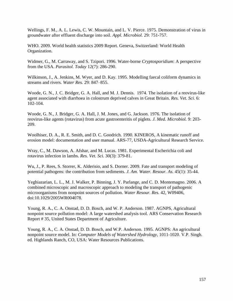
157

Wellings, F. M., A. L. Lewis, C. W. Mountain, and L. V. Pierce. 1975. Demonstration of virus in

groundwater after effluent discharge into soil. Appl. Microbiol. 29: 751-757.

WHO. 2009. World health statistics 2009 Report. Geneva, Switzerland: World Health

Organization.

Widmer, G., M. Carraway, and S. Tzipori. 1996. Water-borne Cryptosporidium: A perspective

from the USA. Parasitol. Today 12(7): 286-290.

Wilkinson, J., A. Jenkins, M. Wyer, and D. Kay. 1995. Modelling faecal coliform dynamics in

streams and rivers. Water Res. 29: 847–855.

Woode, G. N., J. C. Bridger, G. A. Hall, and M. J. Dennis. 1974. The isolation of a reovirus-like

agent associated with diarrhoea in colostrum deprived calves in Great Britain. Res. Vet. Sci. 6:

102-104.

Woode, G. N., J. Bridger, G. A. Hall, J. M. Jones, and G. Jackson. 1976. The isolation of

reovirus-like agents (rotavirus) from acute gastroenteritis of piglets. J. Med. Microbiol. 9: 203-

209.

Woolhiser, D. A., R. E. Smith, and D. C. Goodrich. 1990. KINEROS, A kinematic runoff and

erosion model: documentation and user manual. ARS-77, USDA-Agricultural Research Service.

Wray, C., M. Dawson, A. Afshar, and M. Lucas. 1981. Experimental Escherichia coli and

rotavirus infection in lambs. Res. Vet. Sci. 30(3): 379-81.

Wu, J., P. Rees, S. Storrer, K. Alderisio, and S. Dorner. 2009. Fate and transport modeling of

potential pathogens: the contribution from sediments. J. Am. Water. Resour. As. 45(1): 35-44.

Yeghiazarian, L. L., M. J. Walker, P. Binning, J. Y. Parlange, and C. D. Montemagno. 2006. A

combined microscopic and macroscopic approach to modeling the transport of pathogenic

microorganisms from nonpoint sources of pollution. Water Resour. Res. 42, W09406,

doi:10.1029/2005WR004078.

Young, R. A., C. A. Onstad, D. D. Bosch, and W. P. Anderson. 1987. AGNPS, Agricultural

nonpoint source pollution model: A large watershed analysis tool. ARS Conservation Research

Report # 35, United States Department of Agriculture.

Young, R. A., C. A. Onstad, D. D. Bosch, and W.P. Anderson. 1995. AGNPS: An agricultural

nonpoint source model. In: Computer Models of Watershed Hydrology, 1011-1020. V.P. Singh.

ed. Highlands Ranch, CO, USA: Water Resources Publications.