
Modeling contaminant transport in polyethylene and metal ...
90
Modeling contaminant transport in polyethylene and metal speciation in saliva Jia Tang Thesis submitted to the faculty of the Virginia Polytechnic Institute and State University in partial fulfillment of the requirements for the degree of Masters of Science In Environmental Engineering Andrea M. Dietrich, Chairperson Daniel L. Gallagher Marc A. Edwards June 17, 2010 Blacksburg, Virginia Key words: modeling, polyethylene, geomembrane, diffusivity, solubility, polymer, copper, iron, zinc, artificial saliva, flavor, chemical speciation
Transcript of Modeling contaminant transport in polyethylene and metal ...

Modeling contaminant transport in polyethylene and metal speciation in saliva
Jia Tang
Thesis submitted to the faculty of the
Virginia Polytechnic Institute and State University
in partial fulfillment of the requirements for the degree of
Masters of Science
In
Environmental Engineering
Andrea M. Dietrich, Chairperson
Daniel L. Gallagher
Marc A. Edwards
June 17, 2010
Blacksburg, Virginia
Key words: modeling, polyethylene, geomembrane, diffusivity, solubility, polymer,
copper, iron, zinc, artificial saliva, flavor, chemical speciation

Modeling contaminant transport in polyethylene and metal speciation in saliva
Jia Tang
ABSTRACT
Properties of both chemical contaminants and polymers can impact contaminant
diffusivity and solubility in new and aged polyethylene materials for pipes and
geomembranes. Diffusivity, solubility, polymer and chemical properties were
measured for thirteen contaminants and six polyethylene materials that were new
and/or aged in chlorinated water. Tree regression was used to select variables, and
linear regression was used to develop predictive equations for contaminant
diffusivity and solubility in polyethylene. Organic contaminant properties had
greater predictive capability than polyethylene properties. Model coefficients
significantly changed between new materials to chlorine-aged materials, indicating
changes of polyethylene properties impact the interaction between contaminants
and polymers.
The metallic flavor of copper in drinking water influences the taste of water and
can cause the taste problems for water utilities. The mechanism of metallic flavor
caused by these metals is related to free or soluble ions. Free copper concentrations
were measured at different pH in diluted artificial saliva using a cupric ion
selective electrode. Three major proteins in human saliva: α-amylase, mucin and
lactoferrin, were added in the artificial saliva and the impacts on the chemical
speciation of copper were analyzed. Inorganic saliva components, typically
phosphate, carbonate and hydroxide combined with copper and greatly influenced
the levels of free copper in the oral cavity. Proteins such as α-amylase, mucin and
lactoferrin also impacted the chemical speciation of copper, with different affinity
to copper. Mucin had the greatest affinity with copper than α-amylase.

iii
Acknowledgements
I gratefully thank the National Science Foundation and the Water Research
Foundation for the financial support for this research. Thanks to my committee
members Dr. Andrea Dietrich, Dr. Daniel Gallagher and Dr. Marc Edwards for
their advice, patience, and assistance during these two projects. Thanks Dr. Duncan
and Mr. Robert Moore in food science for their suggestions. Laboratory managers
Julie Petruska and Jody Smiley provided invaluable assistance with equipment and
analytical analysis. Betty Wingate and Beth Lucas help me a lot in purchasing
laboratory supplies and preparing documents. My fellow lab researchers Susan
Mirlohi, Jose Cerrato and Christine Marie Sargent also gave me lots of help in my
experiments. I also thank my friends at Virginia Polytechnic Institute and State
University for assistance, friendship, and supports. Finally, I would like to thank
my family for their support, faith, and endless love.

iv
Author’s Preface & Attribution
This thesis is composed of two manuscripts. Each chapter is a separate manuscript to
which several colleagues contributed. A brief description of their background and their
contributions are included here.
Chapter 1 presents a predictive model and manuscript developed through the integrated
work of Mr. Jia Tang (MS student), Dr. Andrea M. Dietrich, (Professor, Dept. Civil &
Environmental Engineering, Virginia Tech and Committee Chair), and Dr. Daniel L. Gallagher,
P.E. (Associate Professor Dept. Civil & Environmental Engineering, Virginia Tech and
Committee Member). The input data for the model development were obtained from the
dissertation of Dr. Andrew Whelton, who was advised by Drs. Dietrich and Gallagher, and their
published articles.
Chapter 2 was primarily the combined work of Mr. Jia Tang (MS student) and Dr.
Andrea M. Dietrich, (Professor, Dept. Civil & Environmental Engineering, Virginia Tech, and
Committee Chair). They were aided by helpful suggestions and insights from Dr. Marc Edwards,
(Professor, Dept. Civil & Environmental Engineering, Virginia Tech, Committee Member), Dr.
Daniel L. Gallagher, P.E., (Associate Professor Dept. Civil & Environmental Engineering,
Virginia Tech and Committee Member), and Dr. Susan E. Duncan (Professor, Dept. Food
Sciences and Technology, Virginia Tech).

V
Contents
Acknowledgements ...................................................................................................................................... iii
Author’s Preface & Attribution .................................................................................................................... iv
Contents ........................................................................................................................................................ V
List of figures ............................................................................................................................................... VII
List of tables ............................................................................................................................................... VIII
Chapter 1 ....................................................................................................................................................... 1
Abstract ..................................................................................................................................................... 1
Keywords: Modeling, PE pipe, geomembrane, diffusivity, solubility, polymer ........................................ 1
1. Introduction .......................................................................................................................................... 2
2. Materials and Methods ......................................................................................................................... 6
2.1 Experimental laboratory procedures .............................................................................................. 6
2.2 Data for model development and validation .................................................................................. 6
2.3 Tree Regression ............................................................................................................................... 9
2.4 Linear regression ........................................................................................................................... 10
3. Results and discussion ........................................................................................................................ 11
3.1 Evaluating influence of contaminant and PE properties on diffusion and solubility using tree
regression ............................................................................................................................................ 11
3.2 Linear regression ........................................................................................................................... 15
3.3 Model validation ........................................................................................................................... 18
4. Conclusion ........................................................................................................................................... 23
5. References .......................................................................................................................................... 24
Chapter 2 ..................................................................................................................................................... 30
Abstract ................................................................................................................................................... 30
Keywords: Copper, iron, zinc, artificial saliva, flavor, chemical speciation ............................................ 30
1. Introduction ........................................................................................................................................ 31
1.1 Copper, Iron and Zinc for Human Health ...................................................................................... 31
1.2 Standard and Regulation of Copper, Iron and Zinc ....................................................................... 33
1.3 Aesthetics ...................................................................................................................................... 34
1.4 Chemical Speciation of Copper ...................................................................................................... 36
1.5 Composition of Saliva .................................................................................................................... 41

VI
1.6 Role of Saliva in Complexion Metals ............................................................................................. 43
2. Materials and Methods ....................................................................................................................... 46
2.1 Artificial Saliva Solution Preparation ............................................................................................ 46
2.2 Treatment of copper ..................................................................................................................... 47
2.3 Ion Selective Electrode measurement ........................................................................................... 48
2.4 Modeling Metal Speciation ........................................................................................................... 49
3. Results and Discussion ........................................................................................................................ 50
3.1 Predicting Speciation of Cu, Fe and Zn with Inorganic Components of Saliva .............................. 50
3.2 Comparison between measured and MINEQL+ modeled soluble copper in saliva. ...................... 54
3.3 The role of proteins in copper speciation ...................................................................................... 55
3.4 Binding capacity of proteins with copper ...................................................................................... 62
3.5 Changes of pH and free copper in saliva with time. ...................................................................... 63
4. Conclusions and Suggestions ............................................................................................................. 65
5. Reference ............................................................................................................................................ 65
Appendix ..................................................................................................................................................... 72
Abbreviation ............................................................................................................................................ 72
Data for regression model ...................................................................................................................... 73
R codes for regression model .................................................................................................................. 79
New pipe ............................................................................................................................................. 79
Aged pipe ............................................................................................................................................ 79
Experimental data for copper speciation ................................................................................................ 81

VII
List of figures
Figure 1-1 Tree regression for contaminant diffusion in new PE materials; Mv is molecular volume; log
Kow is log octanol-water coefficient; Sw is water solubility. The number in the box represent mean
diffusivity for corresponding group; N= number of data points in group. .................................................. 12
Figure 1-2 Tree regression for contaminant solubility in new PE materials Mu is dipole moment and is a
measure of contaminant polarity; logKow is octanol-water partition coefficient; Sigma is solubility
parameter . The number in the box represent mean diffusivity for corresponding group; N= number of
data points in group. .................................................................................................................................... 13
Figure 1-3 Tree regression for contaminant diffusion in aged PE materials; Mu is dipole moment and is a
measure of contaminant polarity. The number in the box represent mean diffusivity for corresponding
group; N= number of data points in group. ................................................................................................. 14
Figure 1-4 Tree regression for solubility in aged PE materials; Mu is dipole moment and is a measure of
contaminant polarity. The number in the box represent mean diffusivity for corresponding group; N=
number of data points in group. .................................................................................................................. 14
Figure 1-5 Adsorption curves for propanone, 2-butanone, dichloromethane (DCM) and MTBE in 4 PEs.
Data is based on the average values of 3 replicates for each chemical in each PE. .................................... 19
Figure 1-6 Model validation for diffusivity. ............................................................................................... 22
Figure 1-7 Model validation for solubility. ................................................................................................. 23
Figure 2-1 Forms of Copper present in Aquatic Environments (Paulson 1993) ......................................... 38
Figure 2-2 Theoretical copper speciation for hydroxo complexes in pure water for a total copper
concentration of 1 mg/l, which is the value for the USEPA aesthetic-based standard (Cuppett et al. 2006)
.................................................................................................................................................................... 39
Figure 2-3 Schematic structure of mucins(Wu et al. 1994) ........................................................................ 42
Figure 2-4 Free metal ion concentration as a function of pH modeled by MINEQL+; a: inorganic
components of artificial saliva; b: nanopure water; total metal concentration was 10 mg/L as metal........ 51
Figure 2-5 Distribution of free, soluble and precipitate forms of metals in inorganic artificial saliva at
various pH values; A: Copper (Cu2+
); B: Iron (Fe2+
); C: Zinc (Zn2+
) ......................................................... 53
Figure 2-6 Comparison in free copper concentration between measured by copper-ISE (Ion Selective
Eletrode) and modeled by MINEQL+ in 10 mg/L copper in artificial saliva with only inorganic
components; measured data is based on 3 replicates. ................................................................................. 55
Figure 2-7 Free copper in artifical saliva with alpha-amylase .................................................................... 57
Figure 2-8 Free copper in artificial saliva with mucin ................................................................................ 59
Figure 2-9 The impacts of mucin concentration on the free copper concentration in artificial saliva ........ 60
Figure 2-10 The impacts of lactoferrin on the free copper concentration in artificial saliva; data points
represent mean of triplicate measurement; error bars are shown but are not visible .................................. 61
Figure 2-11 Changes in free copper concentration and pH of inorganic artificial saliva with time in 2.5
mg/L of total copper .................................................................................................................................... 64
VIII
List of tables
Table 1-1 Properties of Contaminants Used for Model Development and Validation ................................. 7
Table 1-2 Select Polymer Properties of PE Materials Used for Model Development .................................. 8
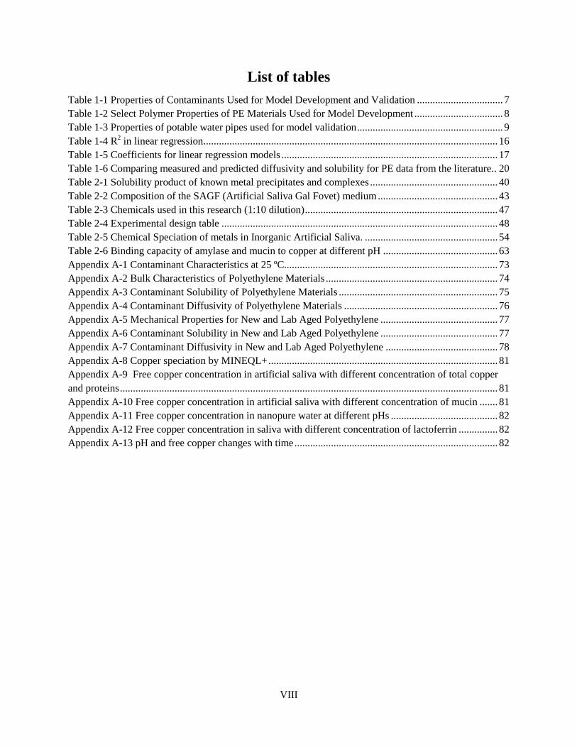
Table 1-3 Properties of potable water pipes used for model validation ........................................................ 9
Table 1-4 R2 in linear regression ................................................................................................................. 16
Table 1-5 Coefficients for linear regression models ................................................................................... 17
Table 1-6 Comparing measured and predicted diffusivity and solubility for PE data from the literature.. 20
Table 2-1 Solubility product of known metal precipitates and complexes ................................................. 40
Table 2-2 Composition of the SAGF (Artificial Saliva Gal Fovet) medium .............................................. 43
Table 2-3 Chemicals used in this research (1:10 dilution) .......................................................................... 47
Table 2-4 Experimental design table .......................................................................................................... 48
Table 2-5 Chemical Speciation of metals in Inorganic Artificial Saliva. ................................................... 54
Table 2-6 Binding capacity of amylase and mucin to copper at different pH ............................................ 63
Appendix A-1 Contaminant Characteristics at 25 ºC.................................................................................. 73
Appendix A-2 Bulk Characteristics of Polyethylene Materials .................................................................. 74
Appendix A-3 Contaminant Solubility of Polyethylene Materials ............................................................. 75
Appendix A-4 Contaminant Diffusivity of Polyethylene Materials ........................................................... 76
Appendix A-5 Mechanical Properties for New and Lab Aged Polyethylene ............................................. 77
Appendix A-6 Contaminant Solubility in New and Lab Aged Polyethylene ............................................. 77
Appendix A-7 Contaminant Diffusivity in New and Lab Aged Polyethylene ........................................... 78
Appendix A-8 Copper speciation by MINEQL+ ........................................................................................ 81
Appendix A-9 Free copper concentration in artificial saliva with different concentration of total copper
and proteins ................................................................................................................................................. 81
Appendix A-10 Free copper concentration in artificial saliva with different concentration of mucin ....... 81
Appendix A-11 Free copper concentration in nanopure water at different pHs ......................................... 82
Appendix A-12 Free copper concentration in saliva with different concentration of lactoferrin ............... 82
Appendix A-13 pH and free copper changes with time .............................................................................. 82

1
Chapter 1
Modeling organic contaminant diffusivity and solubility in polyethylene based
on polymer and organic contaminant properties
Abstract
Properties of both chemical contaminants and polymers can impact contaminant diffusivity and
solubility in new and aged polyethylene (PE) materials for water pipes and geomembranes.
Diffusivity, solubility, polymer and chemical properties were measured for thirteen contaminants
and six PE materials that were new and/or aged in chlorinated water. Tree regression was used to
select variables, and linear regression was used to develop predictive equations for contaminant
diffusivity and solubility in PE. Organic contaminant properties, especially dipole moment and
octanol-water partition coefficient, had greater predictive capability than pipe properties. Values
of R2 > 0.8 were obtained for new and aged pipe. Model coefficients significantly changed
between new PE materials to chlorine-aged PE, indicating changes of PE properties impacted the
interaction between contaminants and PE. Bulk density of PE material played a more important
role for diffusion but had little influence on solubility for both new and aged PE pipes. Diffusion
of polar contaminants was greater in chlorinated water aged polyethylene than new polymers,
although the solubility was similar in both new and aged polymers. These results provide
guidance for material selection and contamination potential for both water pipes and
geomembranes.
Keywords: Modeling, PE pipe, geomembrane, diffusivity, solubility, polymer

2
1. Introduction
Polyethylene (PE) is a polymer that is widely used throughout the world in drinking
water distribution systems and landfill liner applications. PE water pipes are increasingly being
applied in buried and building plumbing globally (AWWA 2003; AWWA 1996). High–density
polyethylene (HDPE) water pipes have been used for buried water service since the 1940s but
their use expanded greatly in the 1990s (AWWSC 2002) and further expanded in the 21st century
with the approval of crosslinked polyethylene (PEX) pipes for buried water service (AWWA
2007). HDPE is also widely used as a geomembrane due to its high short-term chemical
resistance and impermeability liquid wastes (Tisinger et al. 1991; Koerner 1998; Rowe et al.
2004) and excellent mechanical strength (Aminabhavi and Naik, 1998). PE geomembranes are
used as liners for the containment of hazardous and municipal wastes in conjunction with
geotextiles or mesh underliners that allow gases to escape and leachates to be collected. These
PE materials are flexible, inexpensive, resist corrosion, and are expected to provide decades of
service in drinking water systems (Davis et al. 2006) and lifetimes of over 100 years at 35 °C for
HDPE landfill liners (Rowe et al. 2009).
A potential problem for the wide use of PE materials is that organic chemicals can diffuse
in, out, and through PE and adversely affect water quality of drinking water and groundwater.
Aminabhavi and Naik (1999) investigated the transport of 14 non-polar and polar organic
solvents that are frequently found as leachates in landfill and impoundment sites and found that
all of the chemicals permeated PE materials and could result in soil and groundwater
contamination. Non-polar aromatic components of gasoline (benzene and alkylbenzenes) were
demonstrated to permeate HDPE drinking water pipes exposed to gasoline contaminated soil in
the field (Thompson and Jenkins 1987) and under laboratory applications (Mao et al. 2010).
Drinking water distribution systems are vulnerable to intentional or unintentional contamination
with neat solvents or organic contaminants; when this occurs, knowledge of permeation of
contaminant into the polymer pipe is needed to assess the future use of the distribution system
(Clark and Deininger 2002; USEPA 2002). PEs that sorb organic chemicals can also release
them to the water or ambient air resulting in widespread environmental contaminant (Saquing et
al. 2010).

3
Environmental conditions, contaminant properties, and polymer properties affect
diffusivity and solubility of contaminants (Crank and Park 1968; Comyn 1985; Whelton et al.
2010a; Rowe et al. 2009). Increased temperature results in faster diffusion through a polymer and
can also enable polymer chain mobility which increases diffusivity and solubility (Aminabhavi
and Naik 1999). Contaminant diffusion and contaminant dissolution in polymers is restricted to
polymer free volume or amorphous regions, and contaminants do not diffuse through or reside in
highly crystalline/dense regions. Crosslinks generally inhibit contaminant transport and swelling
(Guillot et al. 2004; Desai et al. 1998; Sheu et al. 1989; Haxo et al. 1988) and contaminants can
interact with polymer additives (e.g., carbon black) (Comyn 2004). An increase in PE bulk
density results in a reduction of nonpolar contaminant diffusivity and solubility in PE water pipes
(Dietrich et al. 2010; Whelton et al. 2010a). Contaminant size, shape, symmetry, and polarity can
also influence polymer interactions and polar contaminants are sparingly soluble in hydrophobic
polymers like MDPE and HDPE (Comyn 1985). For instance, polar contaminants (e.g., water,
methanol) are sparingly soluble in hydrophobic polymers (Comyn 1985) whereas nonpolar
compounds (e.g., toluene and trichloromethane) have moderate to great solubility in PEs.
Oxidation of PE from exposure to disinfectant-containing water, oxygen, or leachate can
change polymer surface and bulk properties leading to mechanical failure and changes in
contaminant diffusivity and solubility in PE pipes and liners (Rowe et al. 1999; Dietrich et al.
2010). Two concerns for the drinking water and landfill liner industries are: 1) that the current
state of knowledge concerning PE performance is much less than that of traditional water
distribution materials such as iron and concrete; 2) the effects of PE aging by disinfectants and
oxidation on contaminant permeation in PE are not well understood (Imran et al. 2009).
Differences between new and aged PE surface and bulk characteristics must be
investigated to determine how PE aging impacts contaminant fate and transport. PE water pipes
are known to be attacked by free radicals, including those produced by the disinfectant chlorine
dioxide (Colin et al. 2009 a and b), chlorine (Dietrich et al. 2010; Whelton et al. 2010b; Mitroka
et al. 2010), and oxygenated hot water (Karlsson et al. 1992) resulting in increased polar
carbonyl groups [>C=O] on the surface, loss of antioxidants and oxidative resistance (referred to
as Oxidation Induction Time or OIT) at the surface and in the bulk polymer, and polymer chain
scission that can eventually lead to physical break-down of the polymer (Colin et al. 2009 a and

4
b). HDPE landfill geomembranes exposed to air, water and leachate also exhibit loss of OIT due
to consumption or migration of antioxidants and formation of oxygenated functional groups on
the polymer surface (Rimal and Rowe 2009; Rowe et al. 2009).
Contaminant fate in polymers is dependent on the interactions between the contaminant
and polymer and is commonly described in terms of solubility (S; g/cm3) and diffusivity (D,
cm2/sec) (Crank and Park, 1968). Contaminant solubility can be measured (Equation 1) and
diffusion can be calculated by fitting data to a regression using Equation 2 according to Crank
(1975) as long as the sample thickness is known. Diffusion and solubility have been previously
reported by others to describe neat contaminant interactions with buried HDPE and PEX pipes
and HDPE landfill liners (Dietrich et al. 2010; Whelton et al. 2010a; Chao et al. 2007; Chao et al.
2006; Joo et al. 2005; Joo et al. 2004; Aminabhavi and Naik 1999; Park and Nibras 1993).
Equation 1
Where
M∞ = the mass of contaminant in the saturated polymer (M)
Mp =the initial mass of the polymer (M)
M0 = the initial mass of contaminant in the polymer which is equal to zero (M)
ρ polymer= the polymer’s bulk density (M/L3).
Equation 2
02
22
224
12exp
12
81
n
t tnD
nM
M
Where
Mt = Mass of contaminant in polymer at time t (M)
M∞ = Mass of contaminant in the saturated polymer at equilibrium (M)

5
t = Elapsed time (T)
D = Diffusion coefficient (L2/T)
ℓ = Half sample thickness (L)
There is very little work focused on comprehensive influence of contaminant and PE
properties for predicting contaminant diffusion and solubility in PE materials even though these
materials are vulnerable to chemical contamination that may lead to adverse impacts on water
quality. The goal of this study was to (1) evaluate published data to determine the polymer and
contaminant properties that have essential influence on contaminant diffusion and solubility; (2)
develop a model based on these polymer and contaminant properties to predict contaminant
diffusion and solubility in different PEs; (3) validate the predictive model through application to
other datasets.

6
2. Materials and Methods
2.1 Experimental laboratory procedures
Previous published research from our laboratory provides detailed experimental
procedures for measuring the interaction of contaminants and PEs (Whelton and Dietrich 2009;
Whelton et al 2010a; Dietrich et al. 2010). A brief summary is provided below.
An immersion protocol was used to obtain contaminant diffusivity and solubility values
for new and aged PE materials. Dog-bone shaped PE pieces were cut using a Dewes Gumbs Die
Company, Inc. (Long Island City, NY) microtensile die and triplicate pieces were immersed in
neat contaminant. Immersion testing was conducted by placing PE samples inside screw–tight
amber vials with polytetrafluoroethylene septa containing 15-20 mL of neat contaminant at 22 +
1 °C. Periodically, samples were removed for < 30 seconds, quickly blotted with KimWIPES™
to remove any surface contaminant. Weight measurements were made to 0.0001 g using a
Mettler–Toledo (Columbus, OH) balance until a constant mass was obtained. The thickness of
the PEs was measured using a Mitutoyo electronic outside micrometers (McMaster-Carr).
Laboratory chlorinated-water aged PE samples were exposed on all sides to chlorinated water
containing 45 mg/L free available chlorine (Cl2) and 50 mg/L alkalinity as CaCO3 which was
maintained at pH 6.5, 37 °C and darkness. During aging, water sorption did not occur and the
surface area did not change. The oxidation induction time decreased and carbonyls functional
groups formed on the surface except for PEX-A.
Weight gain over times data was used to calculate solubility and diffusivity coefficients
using Equations 1 and 2. Asymptotic 95% confidence interval was also calculated from the
standard error using R version 2.7.1 (R Development Core Team 2008). Type I error of 0.05 was
applied in all statistical tests.
2.2 Data for model development and validation
Two sets of data were used for this research. The first set was based on measurements
taken in our laboratory and was used to develop the predictive model. The second set was a

7
combination of additional laboratory data as well as literature data. This second set was used to
validate the predictive model.
The predictive model was developed based on previously reported for contaminant solubility and
diffusivity data from our research group (Whelton et al. 2009; Dietrich et al 2010; Whelton et al
2010a). The thirteen non-polar and polar contaminants and six of their physical/chemical
properties are presented in Table 1-1.
Table 1-1 Properties of Contaminants Used for Model Development and Validation.
Contaminant
Contaminant Property1
Mμ,
Debye
Mv,
cm3
Mm,
g/mol
Sw,
%
ρ,
g/cm3
Log
Kow
Polar
Acetonitrile 3.92 53.3 41.05 100 0.786 -0.34
2–Propanone2,3
2.88 73.1 58.08 100 0.789 -0.24
Benzaldehyde2 2.80 120.5 106.12 0.3 1.041 1.48
2–Butanone2,3
2.76 91.4 72.11 22.3 0.805 0.29
Benzyl Alcohol2 1.71 125.1 108.14 4 1.041 1.10
1–Butanol2 1.66 96.2 74.12 7.4 0.809 -0.30
2–Propanol2 1.56 77.8 60.10 100 0.789 0.05
Nonpolar
Dichloromethane3 1.60 60.6 84.93 1.303 1.326 1.25
MTBE2,3
1.36 119.1 88.15 5.1 0.740 1.24
Trichloromethane2,3
1.01 74.4 119.37 0.729 1.492 1.97
Toluene2,3
0.36 117.7 92.14 0.0526 0.867 2.73
m–Xylene2 0.30 135.9 106.16 0.0161 0.864 3.20
p–Xylene 0.00 135.8 106.16 0.0162 0.867 3.15
1. Mμ is dipole moment; Mv is molecular volume; Mm is molecular weight; Sw is water solubility; Log Kow
is octanol-water partition coefficient.
2. These ten contaminants were tested in aged PEs; all thirteen contaminants were tested in new PE materials;
3. These four contaminants were used for model validation. Contaminants listed for both development and
validation used different PE samples for each.
Six polyethylene materials were evaluated. HDPE resin sheets were obtained from McMaster–
Carr, Inc. (Atlanta, GA) and new HDPE, PEX–A, and PEX–B pipes were obtained from a
commercial supplier. Six parameters were determined for new and chlorine-aged PE pipes:
tensile strength at break, tensile strength at yield, elongation, OIT, bulk density, crystallinity; an
additional four parameters were measured for new PE materials: crosslink density, temperature
of degradation, thickness, and polymer percentage (Dietrich et al. 2010; Whelton et al. 2010a and
b). The bulk density and OIT values are presented in Table 1-2 as only these two values are
important to the results and discussion.

8
Table 1-2 Select Polymer Properties of PE Materials Used for Model Development.
PE Material Pipe
Age
Bulk Density
(g/cm3)
Oxidation
Induction Time
(OIT) (min)
Resin New 0.9578 22.4
Aged 0.9581 13.5
Monomodal HDPE New 0.9494 92.5
Aged 0.9513 29.7
Bimodal HDPE New 0.9547 119.6
PEX-A New 0.9385 33.5
Aged 0.9389 27.2
PEX-B (1) New 0.9524 119.6
Aged 0.9527 5.4
PEX-B (2) New 0.9510 > 295
Literature data for diffusivity and solubility of organic contaminants in PEs was used to
verify the model. Due to the lack of diffusivity and solubility data for polar compounds in
literature, new diffusivity and solubility data for one new PE and 3 aged PEs taken from a
potable water distribution system, which are listed in Table 1-3, were measured in this research
to verify the model. The organic chemicals used were 2-propanone, 2-butanone, MTBE, and
dichloromethane, the properties of which are listed in Table 1-1.
9
Table 1-3 Properties of potable water pipes used for model validation.
Pipe Material Density
(g/cm3)
Pipe Characteristics
PE 1 0.9551 New HDPE pipe
PE 22 0.9504
7 years in service in water
distribution system that only
applied combined chlorine
PE 32 0.9513
20 years in service in a water
distribution system :18 years free
available chlorinated water and 2
years exposure to chloramines
chloramines combined chlorine)
PE 42 0.9504
25 years in service in a water
distribution system that only
applied free available chlorine
1. Data provided by manufacturer.
2. Data from Dietrich et al. 2010.
2.3 Tree Regression
Tree regression (Lewis 2000; Venables and Ripley 2002; Crawley 2007; Zuur et al 2007;
Cheng, Zhang et al. 2009) were generated in R to determine which contaminant and PE property
had the greatest effect on contaminant transport. Constructing tree regressions may be seen as a
type of variable selection because regression trees indicate the relative importance and
interactions of the different factors. Regression trees are a type of predictive model that
progressively select the critical regression variables in the order of their impact, or importance, to
the model. In the first step, the regression splits the data into two groups or branch based on the
most important variable. Tree regressions used for this analysis use binary recursive partitioning
to sequentially split the data into two branches so that the difference in the response variable
(solubility or diffusivity) between the two branches is greatest. The tree construction process
takes the maximum reduction in deviance over all allowed splits of all leaves to choose the next
split. The approach is computationally intensive because each split calculates the possible
deviance reduction for all possible values of all explanatory variables.

10
In this study, tree regressions, in which the independent variables comprised both the
organic contaminant properties (dipole moment, molecular volume, molecular weight, water
solubility, density, octanol-water partition coefficient etc.) and PE material properties (density,
oxidation induction time, crystallinity etc.), were performed separately for diffusion and
solubility for both new pipe and aged pipe. The results of tree regressions visually demonstrated
the significant variables for diffusion and solubility and provided for variable selection for the
models.
2.4 Linear regression
In this study, a multiple regression with maximum sixteen independent variables
containing six contaminant properties (Table 1-1) and ten polymer properties for new PE pipe
and only six polymer properties for aged pipe were used to build the model.
The dependent variables were diffusion coefficients and solubility (6 PEs x 13
contaminants = 78 for new pipes; 4 PEs x 10 contaminants = 40 for aged pipes);the independent
variables consisted of contaminant and pipe properties (6 contaminant properties + 10 pipes
properties = for new pipes and 6 contaminant properties + 6 pipes properties = 12 for aged pipes).
An indicator variable with 0 for new pipe and 1 for aged pipe was created to determine the
changes in slopes and intercepts of the models after pipes were exposed to chlorinated water.
Variables were selected based on the correlation between each other, the p value of the
slope for each variable, results of tree regressions, and the contribution to the multiple R square
for the regression model. Residuals analysis was used to illustrate the goodness of the regression
and to check regression assumptions.
A two tailed paired t-test (α =0.05) was used to compare the validation data set of
previously published data in literature and our laboratory experiment with the predicted data
from our models.

11
3. Results and discussion
3.1 Evaluating influence of contaminant and PE properties on diffusion and solubility using
tree regression
The contaminant solubility and diffusivity data for new PE materials used to develop this
model were previously published (Whelton et al. 2010a); data for contaminant interactions with
aged PE materials are also published (Dietrich et al, 2010; Whelton 2009; Whelton et al. 2010b).
Figure 1-1 shows the tree regression result for the contaminant diffusion in new PE materials.
The interpretation of the regression indicates that diffusion was principally and equally
controlled by either by water solubility or log Kow of the organic contaminants. At high water
solubility (Sw>=2.65%) or low octanol-water partition coefficient (log Kow<1.245), the
diffusivity value averaged 7.275 (*10-9
cm2/s). At low water solubility (Sw<2.65%) or high
octanol-water coefficient (log Kow>=1.245), molecular volume also became an important factor.
These results could be explained from a chemical perspective: lower water solubility and high
octanol-water coefficient are associated with more hydrophobic compounds which are more
soluble in PE materials than water; small molecular volumes allowed non-polar molecules to
more easily penetrate into the free volume or amorphous regions of PE. This trend was also
reported by Joo et al. (2005).

12
Figure 1-1 Tree regression for contaminant diffusion in new PE materials; Mv is molecular volume; log Kow
is log octanol-water coefficient; Sw is water solubility. The number in the box represent mean diffusivity for
corresponding group; N= number of data points in group.
The tree regression result for the contaminant solubility in new PE materials is shown in
Figure 1-2. The octanol-water partition coefficient, which is a ratio of the solubility of a
contaminant in non-polar octanol and polar water and typically reported as LogKow, is the
principal property. At higher logKow (>1.17), which indicates the contamiant is more soluble in
non-polar materials, chemical polarity, as measured by dipole moment, played an important role.
Low polarity chemicals (μ<1.185) had stronger interaction with non-polar polymers, which
resulted in higher solubility in PE materials. However, solubility did not increase continuously
with the decrease of polarity, but decreased after dipole moment fell below Mu= 0.33. To
interpret this phenomenon, the properties of the polymers needs to be considered. The polarity of
the polymer is not likely zero because its structure is not absolutely symetrical (Sahebiana et al.
2009) and presence of phenolic antioxidants or X-linking. Thus, contaminants with very low
polarity (Mu<0.33) or absolutely no polarity did not interact with polymers as well as those
contaminants which have similar polarity with the polymer. In the third node of this figure,
several parameters including dipole moment, solubility parameter, molecular volume etc equally
divided the node with 24 data points. This may due to the repetition of these parameter in the
solubility data with the same organic contaminants or the same PE materials. This cannot
distinguish the order of importance of these parameters because the total data points is limited.

13
.
Figure 1-2 Tree regression for contaminant solubility in new PE materials Mu is dipole moment and is a
measure of contaminant polarity; logKow is octanol-water partition coefficient; Sigma is solubility
parameter . The number in the box represent mean diffusivity for corresponding group; N= number of data
points in group.
Figure 1-3 and Figure 1-4 show the tree regressions for diffusion and solubility in aged
PE pipe. In both figures, water solubility no longer plays an important role and contaminant
polarity, as measured by dipole moment or octanol-water partition coefficient, was the dominant
factor controlling the diffusion and solubility. Similar to the effect of contaminant polarity in
new PE pipe, there is not a linear relationship between contaminant polarity and diffusion as well
as solubility, but a trend of decreasing and then increasing diffusion and solubility with the
increasing of contaminant polarity. The surface oxidation of polymers may contribute to this
result. As polar groups ((>C=O,–OH etc.) were produced and polymer chain scission occurred in
disinfected water, the PE surface become more polar (Colin et al. 2009; Whelton and Dietrich
2009; Dietrich et al. 2010), which increased the importance of polarity in contaminant diffusion
and solubility.

14
Figure 1-3 Tree regression for contaminant diffusion in aged PE materials; Mu is dipole moment and is a
measure of contaminant polarity. The number in the box represent mean diffusivity for corresponding group;
N= number of data points in group.
`
Figure 1-4 Tree regression for solubility in aged PE materials; Mu is dipole moment and is a measure of
contaminant polarity. The number in the box represent mean diffusivity for corresponding group; N=
number of data points in group.

15
3.2 Linear regression
Variable selection
Tree regression is the first step to select variables but the approach is not suited for
predictive modeling except in the broadest sense. For sixteen variables of new pipe and twelve
of aged pipe, a correlation matrix of these explanatory variables was created to check the
correlation between each variable pair and those with high correlation coefficient were taken out.
After this step, linear regressions were run in R based on the remaining variables. According to
the p value for each coefficient (slope and intercept) and the contribution to R2, three properties
(molecular polarity, molecular volume and octanol-water partition coefficient) of organic
chemical and one property (bulk density) of polymer were chosen for the final model (Table 1-4).
Bulk density of the PE material played a more important role for diffusion but had little
influence on solubility for both new and aged PE pipes. R2 for regressions with bulk density as a
factor was only 0.05 greater than that without bulk density for diffusion in new pipe while there
was only 0.01 increase for solubility, which indicated that bulk density was more important in
predicting diffusion than predicting solubility. For aged pipe, the same result was found. This
finding was expected since diffusion is a process of the contaminant penetrating into the polymer
and it is impacted by the physical pore space of the polymer which is related to bulk density,
while solubility is the chemical state of contaminant interaction with the polymer. Interestingly,
OIT had no role in predicting contaminant diffusion or solubility even though this property in
acknowledged to change greatly in new and aged pipe materials (Table 1-2) and geomembranes
(Rowe et al. 2009).

16
Table 1-4 R2 in linear regression.
New PE Variables in Model R2
Diffusion Mμ Mv Log Kow 0.777
Mμ Mv Log Kow Bulk density 0.828
Solubility Mμ Mv Log Kow 0.851
Mμ Mv Log Kow Bulk density 0.860
Aged PE
Diffusion Mμ Mv Log Kow 0.749
Mμ Mv Log Kow Bulk density 0.817
Solubility Mμ Mv Log Kow 0.835
Mμ Mv Log Kow Bulk density 0.845
Mμ is dipole moment; Mv is molecular volume; log Kow is octanol-water partition coefficient.
Model equations
The relationship between contaminant diffusion and solubility in PE pipe and selected
variables was established by linear regression. Data in Table 1-5 presents the coefficients of all
the intercepts and slopes for these models expressed by the following equation.
The negative and positive signs of the coefficients indicated that both diffusion and solubility
decreased with the increasing of polarity and molecular volume but increased with increasing
octanol-water partition coefficient for both new and aged pipes, which agreed with the finding by
other researchers (Berens and Hopfenberg 1982; Islam et al. 2008; Müller et al. 1998; Sangam
and Rowe 2001, 2005; Joo et al. 2004, 2005). These results can be explained by chemical and
physical interactions. Weak-polar or non-polar contaminants have strong interaction with
polymers which are also weak-polar or non-polar. Small molecules with small molecular
volumes can easily penetrate polymers and also easily stay in the pore cavities of polymers,
resulting in the high diffusion and solubility. Higher octanol-water partition coefficient means
lower water solubility of contaminants which trends to be compatible with polymers.

17
Table 1-5 Coefficients for linear regression models.
Models Model Coefficients
Intercept Mμ Mv Log Kow Bulk density R2
Diffusion in New pipe 1141.0 -7.21 -0.943 25.06 -1092.0 0.828
Diffusion in Aged pipe 979.6 -4.24 -0.718 22.38 -947.4 0.817
Change -161.8*
(-14%)
2.97*
(41%)
0.225*
(24%)
-2.68*
(-11%)
144.5*
(13%) -
Solubility in New pipe 0.7174 -0.0113 -0.0011 0.0358 -0.6163 0.860
Solubility in Aged pipe 0.7363 -0.0059 -0.0013 0.0405 -0.6274 0.845
Change 0.0189*
(3%)
0.0054*
(48%)
-0.0002*
(-18%)
0.0047*
(13%)
-0.0111*
(-2%) -
1.* Significant different from 0 (p>0.05); units of diffusion, solubility, dipole moment, molecular volume, Log Kow
and polymer density are 10-9
cm2/s, g/cm
3, Debye, cm
3/mol, and g/cm
3 respectively.
2. R2s of the Regression based on all 19 variables only increased slightly compared with that based on 4 variables.
Comparison between new and aged pipe
By comparing the coefficients of these models between new and aged pipe, the impact of
parameters on contaminant-polymer interactions can be analyzed and understood. All the
changes of intercepts and slopes were significantly different from 0 (p>0.05), indicating that the
aging of PE materials impacted the interactions between contaminants and polymers. The
solubility and diffusion for new and aged PE materials cannot be modeled by one single equation.
Specifically, the intercept for diffusion decreased from new pipe to aged pipe,
coefficients for polarity, molecular volume and bulk density increased, while the coefficient for
log Kow decreased. Since slopes for polarity, molecular volume and bulk density were negative,
they decreased with respect to absolute value. All decreasing coefficients demonstrated that the
diffusion trended to be uniform for aged PE materials, changing slowly with the change of
selected factors of influence. However, it is hard to say which was greater between new and aged
PEs, since they were depended on the relative values of these properties considered. Islam and
Rowe (2008; 2009) found that the diffusive migration of aqueous VOCs through HDPE
geomembrane was less for an aged geomembrane than for a new geomembrane, while Dietrich
et al. 2010 and Whelton et al. 2010b reported that the neat contaminant diffusion through new
HDPE materials was greater than aged HDPE materials. For solubility, the intercept and

18
coefficients for molecular volume and octanol-water partition coefficient increased, while
coefficient for polarity decreased, all with respect to the absolute value. Therefore, aging seemed
to weaken the influence of polarity on solubility, which appears to conflict with the results of
tree regression. However, the p-value for coefficient of polarity for aged PE materials was 0.228,
which was greater than 0.05, indicating a weak linear relationship between contaminant polarity
and solubility in PEs. Therefore, polarity had a complex impact on contaminant solubility in PEs
rather than linear correlation.
R2 values for both diffusion and solubility regressions reduced about 0.01 from new to
aged PE. This slight decrease demonstrated that the oxidation of polymers raised the complexity
of the interactions between contaminants and polymers.
3.3 Model validation
For all the linear regressions, R2 were greater than 0.8, which displayed acceptable
reliability of this model based on experimental data. Joo et al. (2005) reported that mass transport
parameters of contaminants through a HDPE geomembrane could be estimated by the properties
of organic contaminants such as octanol-water partition coefficient, aqueous solubility, and
molecular diameter, which agreed with our finding. Unfortunately, a high R2 value does not
guarantee that the model will be predictive for data of other researchers. Therefore, several sets
of contaminant diffusion and solubility data from previous work of other researchers and
additional data from our laboratory (Figure 1-5) were investigated and compared with those
calculated by this model.

19
Figure 1-5 Adsorption curves for propanone, 2-butanone, dichloromethane (DCM) and MTBE in 4 PEs. Data
is based on the average values of 3 replicates for each chemical in each PE.

20
Table 1-6 Comparing measured and predicted diffusivity and solubility for PE data from the literature. A
two tailed t-test was used for comparison and data were not significantly different (p>0.05).
Contaminant Diffusivity, 10
-7cm
2/s Solubility, g/cm
3
Measured Predicted Measured Predicted
Dichloromethane 0.87(1)
0.63 0.08(1)
0.09
0.82(2)
0.63 0.12(2)
0.09
0.85(4)
0.57 0.0767(4)
0.1024
1.09(4)
0.56 0.0748(4)
0.1019
0.71(4)
0.57 0.0753(4)
0.1024
0.69(4)
0.61 0.0754(4)
0.0888
0.27(1)
0.52 0.05(1)
0.07
0.42(2)
0.52 0.06(2)
0.07
Trichloromethane 0.51(1)
0.69 0.14(1)
0.10
0.79(3)
0.69
Toluene 0.61(1)
0.71 0.09(1)
0.11
0.68(2)
0.71 0.11(2)
0.11
0.53(3)
0.71
2-Butanone 0.10(4)
0.097 0.0166(4)
0.0190
0.13(4)
0.088 0.0162(4)
0.0185
0.08(4)
0.097 0.0163(4)
0.0190
0.08(4)
0.010 0.0163(4)
0.0095
MTBE 0.055(4)
0.16 0.0562(4)
0.0274
0.104(4)
0.148 0.0472(4)
0.0268
0.054(4)
0.157 0.0479(4)
0.0274
0.057(4)
0.071 0.0489(4)
0.0268
2-Propanone 0.129(4)
0.089 0.0083(4)
0.0179
0.146(4)
0.080 0.0087(4)
0.0173
0.090(4)
0.089 0.0084(4)
0.0178
0.091(4)
0.020 0.0100(4)
0.0067
P of t-test 0.3865 0.8617

21
(1). Chao KP; Wang P; Wang YT. 2007. Diffusion coefficients and solubility coefficients of aromatic and
chlorinated hydrocarbons in HDPE geomembranes were obtained using the steady state permeation and sorption
data from ASTM F739 and immersion methods, respectively;
(2). Aminabhavi TM; Naik HG. 1999. Aminabhavi et al. measured and calculated diffusivities of 14 organic liquids
in HDPE geomembranes;
(3). Dietrich AM; Whelton AJ; Gallagher DL. 2010. Dietrich et al. measured diffusivity and solubility for aged
HDPE pipes removed from disinfected drinking water distribution systems;
(4). The measured data are from experiments in this research.
Although all the data used to develop the predictive model and its validation used the same
immersion method, different researchers determined different diffusivities and solubilities data,
which might result from slight difference of experimental conditions. A two tailed paired t-test
was used for comparing the literature experimental data with fitted data in the regression models,
results of which were displayed in Table 1-6. All the measured experimental data and fitted data
were not significant different (p>0.05), indicating that the model is a good predictor of the
contaminant diffusion and solubility.
Further validation was conducted by regressing the predicted versus measured/literature values
for the validation set (Figures 1-6 and 1-7). For both diffusivity and solubility, the slopes were
not significantly different than 1 and the intercepts were not significantly different than 0,
indicating that the predictive model is suitable for predicting solubilities and diffusivities of
contaminant-PE pairs not in the original calibration data set. The residual standard errors, a
measure of the average error between predicted and measured values, were 0.17 (10-7
cm2/s) and
0.019 (g/cm3) for diffusivity and solubility respectively.

22
Figure 1-6 Model validation for diffusivity.
0.0 0.2 0.4 0.6 0.8 1.0
0.0
0.2
0.4
0.6
0.8
1.0
D predicted (10-7 cm2/s)
D m
ea
su
red
(1
0-7
cm
2/s
)
regression
1:1

23
Figure 1- 7 Model validation for solubility.
4. Conclusion
Neat contaminant diffusion and solubility in new and aged polyethylene can be predicted based
on the properties of both contaminants and polymers. The contaminant properties of water
solubility, octanol-water partition coefficient and molecular volume were major determinants for
contaminant solubility and diffusivity; PE bulk density played a minor role with less dense
polyethylene materials more susceptible to contamination. The coefficients of the models
demonstrated that the aging of PE materials impacted the interactions between contaminants and
0.00 0.05 0.10 0.15
0.0
00
.05
0.1
00
.15
S predicted (g/cm3)
S m
ea
su
red
(g
/cm
3)
regression
1:1

24
polymers. Bulk density of PE material played a more important role for diffusion but had little
influence on solubility for both new and aged PE pipes. Polar contaminants diffused faster into
chlorinated water aged polyethylene, although the solubility was similar in both new and aged
polymers. Two predictive equations are necessary because of the significant differences between
new and aged HDPE materials.
These results will aid in selecting materials for both pipes and geomembrane liners and assessing
contamination potential in PEs.
5. References
American Water Works Association (AWWA). 2007. Standard C904–06 crosslinked
polyethylene (PEX) pressure pipe, ½ in (12 mm) through 3 in. (76mm), for water service.
Denver, CO.
AWWA. 2003. AWWA Water Stats Survey/Database. Denver, CO.
American Water Works Service Company Inc. (AWWSC). 2002. Deteriorating Buried
Infrastructure, Management Challenges and Strategies. Prepared for the Environmental
Protection Agency. Washington, DC; available at:
http://www.epa.gov/safewater/disinfection/tcr/pdfs/whitepaper_tcr_infrastructure.pdf.
Aminabhavi TM; Naik HG. 1999. Sorption/desorption, diffusion, permeation and swelling of
high density polyethylene geomembrane in the presence of hazardous organic liquids. Jour.
Haz. Mat. B(64), 251-262.
Aminabhavi TM; Naik HG. 1998. Chemical compatibility study of geomembranes—
sorption/desorption, diffusion and swelling phenomena. Journal of Hazardous Materials.
60(2), 175-203.
Arima O; Hasegawa Y. 1991. Estimation of durability of SUMIKEI PEX tubes to residual
chlorine in tap water. Sumitomo Keikinzoku giho. 32(2), 143-148.
Bakır B; Batmaz İ; Güntürkün FA; İpekçi İA; Köksal G and Özdemirel NE. 2006. Defect cause
modeling with decision tree and regression analysis. Proceedings of World Academy of
Science, Engineering and Technology. 17. 266-269.

25
Berens AR; Hopfenberg HB. 1982. Diffusion of organic vapors at low concentration in glassy
PVC, PS and PMMA. J. Membr. Sci. 10(2–3), 283-296.
Chao KP; Wang P; Wang YT. 2007. Diffusion and solubility coefficients determined by
permeation and immersion experiments for organic solvents in HDPE geomembrane. Journal
of Hazardous Materials. 142(1-2), 227-235.
Cheng W; Zhang XY et al. 2009. Integrating classification and regression tree (CART) with GIS
for assessment of heavy metals pollution. Environmental Monitoring and Assessment. 158(1-
4): 419-431.
Clark RM &. Deininger RA. 2002. Protecting the nation's critical infrastructure: the
vulnerability of U.S. water supply systems. Journal of Contingencies and Crisis Management.
8 (2) 73 - 80
Colin X; Audouin L; Verdu J; Rozental-Evesque M; Rabaud B; Martin F; Bourgine F. 2009.
Aging of polyethylene pipes transporting drinking water disinfected by chlorine dioxide. I.
Chemical aspects. Polymer Engineering & Science. 49(7), 1429-1437.
Colin X; Audouin L; Verdu J; Rozental-Evesque M; Rabaud B; Martin F; Bourgine F. 2009.
Aging of polyethylene pipes transporting drinking water disinfected by chlorine dioxide. Part
II - Lifetime prediction. Polymer Engineering & Science. 49(8), 1642 – 1652.
Comyn J. (ed.). 2004. Polymer Permeability. Elsevier Sci. Pub. Co. New York, NY.
Crank JS; Park GS. 1968. Diffusion in Polymers. Academic Press Inc. New York, NY.
Crank. 1975. The Mathematics of Diffusion. Oxford - Clarendon Press. Oxford, United Kingdom.
Crawley, M. J. 2007. The R Book. John Wiley & Sons, Chichester, England.
Davis P; Burn S; Gould S; Cardy M; Tjandraatmadja G; Sadler P. 2006. Final Report: Long term
performance prediction for PE pipes. AwwaRF. Denver, CO USA.
Desai S; Thakore IM; Devi S. 1998. Effect of crosslink density on transport of industrial solvents
through polyether based polyurethanes. Poly. Intl. 47, 172-178.

26
Dietrich AM; Whelton AJ; Gallagher DL. 2010. Evaluating Critical Relationships Between New
and Aged Polyethylene Water Pipe and Drinking Water Contaminants Using Advanced
Material Characterization Techniques, Final Report. Water Research Foundation, Denver,
CO [In Press]
Guilliot S; Briand E; Galy J; Gerard J–F; Larroque M. 2004. Relationship between migration
potential and structural parameters in crosslinked polyethylenes. Polym. 45(22), 7739-7746.
Gedde UW; Viebke H; Leijstrom H; Ifwarson M. 1994. Long–term properties of hot water
polyolefin pipes—A review. Poly. Eng. Sci. 34(24), 1773-1787.
Haxo HE Jr.; Lahey TP. 1988. Transport of dissolved organics from dilute aqueous solutions
through flexible membrane liners. Haz. Waste and Haz. Mat. 5(4), 275-294.
Imran S; Sadiq R; Kleiner Y. 2009. Effect of regulations and treatment technologies on
distribution system infrastructure. J. Amer. Water Works Assoc. 101(3), 82-95.
Islam MZ; Rowe RK. 2008. Effect of Geomembrane Ageing on the Diffusion of VOCS through
HDPE Geomembranes. The First Pan American Geosynthetics Conference & Exhibition. 2-5
March 2008, Cancun, Mexico.
Islam MZ; Rowe RK. 2009. Permeation of BTEX through Unaged and Aged HDPE
Geomembranes. Journal of Geotechnical and Geoenvironmental Engineering 135(8): 1130-
1140.
Joo JC; Nam K; Kim JY 2005. Estimation of mass transport parameters of organic compounds
through high density polyethylene geomembranes using a modified double–compartment
apparatus. Journ. Env. Engr. 131(5), 790-799.
Joo JC; Kim JY; Nam K. 2004. Mass transfer of organic compounds in dilute aqueous solutions
into high density polyethylene geomembranes. Journ. Env. Engr. 130(2), 175-183.
Karlsson K; Smith GD; Gedde UW. 1992. Molecular structure, morphology, and antioxidant
consumption in medium density polyethylene pipes in hot-water applications. Polym. Eng.
Sci. 32(10), 649-657.

27
Koerner RM. 1998. Designing with Geosynthetics, 4th edition. Prentice Hall, New Jersey, 761
pp.
Lewis RJ. 2000. An Introduction to Classification and Regression Tree (CART) Analysis. 2000.
Annual Meeting of the Society for Academic Emergency Medicine in San Francisco,
California.
Mao F; Gaunt JA; Cheng C-L; Ong SK. 2010. Permeation of BTEX compounds through HDPE
pipes under simulated field conditions. Journal of the American Water Works Association,
102(3) 107-118.
Mitroka S; 2010. Modulation of hydroxyl radical reactivity and radical degradation of high
density polyethylene. Dissertation. Dr. James Tanko, advisor. Department of Chemistry,
Virginia Tech, Blacksburg, VA
Müller W; Jacob L; Tatzky GR; August H. 1998. Solubilities, diffusion and partitioning
coefficients of organic pollutants in HDPE geomembranes: experimental results and
calculations, Proceedings of the 6th International Conference on Geosynthetics, Atlanta, 239-
248.
Park JK; Nibras M. 1993. Mass flux of organic chemicals through polyethylene geomembranes.
Wat. Env. Res. 65(3), 227-237.
R Development Core Team (2008). R: A language and environment for statistical computing. R
Foundation for Statistical Computing, Vienna, Austria. ISBN 3–900051–07–0, URL
http://www.R–project.org.
Rimal S; Rowe RK. 2009. Diffusion modelling of OIT depletion from HDPE geomembrane in
landfill applications. Geosynthetics International. 16(3), 183-196.
Roger J; Lewis MD. An Introduction to Classification and Regression Tree (CART) Analysis.
Harbor-UCLA Medical Center. Torrance, California.
Rowe RK; Rimal S; Sangam H. 2009. Ageing of HDPE geomembrane exposed to air, water and
leachate at different temperatures. Geotextiles and Geomembranes. 27, 137-151.

28
Sahebiana S; Zebarjada SM; Vahdati Khakia J; Sajjadia SA. 2009. The effect of nano-sized
calcium carbonate on thermodynamic parameters of HDPE. Journal of Materials Processing
Technology. 209(3), 1310-1317.
Sangam HP; Rowe RK. 2001. Migration of dilute aqueous organic pollutants through HDPE
geomembranes. Geotextiles and Geomembranes. 19(6), 329-357.
Sangam HP; Rowe RK. 2005. Effect of surface fluorination on diffusion through a high density
geomembrane. Journal of Geotechnical and Geoenvironmental Engineering. 131(6), 694-704.
Saquing JM; Mitchel LA; Wu B; Wagner TB; Knappe DRU; Barlaz MA. 2010. Factors
controlling alkylbenzene and tetrachloroethene desorption from municipal solid waste
components. Environ. Sci. Technol. 44 (3), 1123–1129.
Thompson C; Jenkins D. 1987. Review of Water Industry Plastic Pipe Practices. AWWARF,
Denver, CO USA.
Tisinger LG; Peggs ID; Haxo HE. 1991. Chemical compatibility testing of geomembranes. In:
Geomembranes Identification and Performance Testing, Rollin, A. and Rigo, J. M., editors,
Chapman and Hall, London, Rilem Report 4, 268–307.
USEPA. 2002. Permeation and Leaching. Washington, DC. Available at:
http://www.epa.gov/safewater/disinfection/tcr/pdfs/whitepaper_tcr_permation-leaching.pdf
Venables WN, Ripley BD. 2002. Modern Applied Statistics with S. Fourth edition. Springer.
New York.
Whelton AJ; Dietrich AM. 2009. Critical considerations for the accelerated aging of
polyethylene potable water materials. Polym. Degrad. Stab. 94(7), 1163-1175.
Whelton AJ; Gallagher DL; Dietrich AM. 2010a. Contaminant diffusion, solubility, and material
property differences between HDPE and PEX potable water pipes. ASCE Journal of
Environmental Engineering, 136(2), 227-237.

29
Whelton AJ; Gallagher DL; Dietrich AM. 2010b. Impact of Chlorinated Water Exposure on
Chemical Diffusivity and Solubility, Surface and Bulk Properties of HDPE and PEX Potable
Water Pipe. Submitted to Journal of Environmental Engineering.
Whelton AJ. 2009. Advancing potable water infrastructure through improved understanding of
polymer pipe oxidation, polymer–contaminant interactions, and consumer perception of taste.
Dissertation; Dr. Andrea M. Dietrich, advisor. Department of Civil and Environmental
Engineering, Virginia Tech. Blacksburg, VA.
Zuur AF; Ieno EN; Smith GM. 2007. Analysing Ecological Data. Springer. New York.

30
Chapter 2
Chemical speciation of metals in artificial saliva
Abstract
The metallic flavor of copper, iron and zinc in drinking water influences the taste of water and
arouses a taste problem for water utilities. The mechanism of metallic flavor caused by these
metals is unclear, but previous researchers reported the importance of free or soluble ions on the
taste intensity of these three metals, which reflects on the thresholds of metals in different forms
of solutions, soluble species or precipitates. Free copper concentrations were measured at
different pH values in diluted artificial saliva using a cupric ion selective electrode. Three major
proteins in human saliva; α-amylase, mucin and lactoferrin were added to the artificial saliva and
their impacts on the chemical speciation of copper were analyzed. Inorganic components,
typically phosphate, carbonate and hydroxide combined with copper and greatly influenced the
levels of free copper in oral cavity. Proteins such as α-amylase, mucin and lactoferrin also
impacted the chemical speciation of copper, with different affinity to copper. Mucin had the
greatest affinity with copper, followed by α-amylase, while lactoferrin had very weak binding
capacity. Inorganic components dominated in the chemical speciation of copper when no levels
of mucin existed in artificial saliva. When the concentration of mucin was raised to > 0.216 mg/L,
free copper is controlled by the concentration of mucin.
Keywords: Copper, iron, zinc, artificial saliva, flavor, chemical speciation
31
1. Introduction
1.1 Copper, Iron and Zinc for Human Health
Copper is an essential element necessary for enzymes and proteins indispensable for life,
and adverse health effects may happen due to deficient or excess in copper intake (Dameron
1998). World Health Organization (WHO) recommends a daily intake of 30 µg/kg body weight
(WHO 1998). Copper deficiency is a well-documented cause of neurologic disease and
hematologic abnormalities (anemia, neutropenia, and leukopenia) in adults known of for many
years. In newborns, copper deficiency can cause devastating neurologic disease, most often
being seen in Menkes disease (Griffith et al. 2009). Besides the lack of sufficient source of
copper intake, copper deficiency can be caused by chronic excessive zinc consumption, such as
may occur in those who overuse denture adhesive compounds, because zinc competes with
copper for absorption by the gut. From available data on human exposures worldwide,
particularly in Europe and the Americas, the risk of health effects from deficiency of copper
intake exceeds that from excess copper intake (Dameron 1998).
Copper levels in seawater of 0.15 µg/L and in fresh water of 1-20 µg/L are found in
undefiled areas (Dameron 1998). Human activities increase the copper concentrations, and the
major sources of release are mining operations, agriculture, solid waste and sludge from
treatment works. However, unlike the relatively low range of µg/L concentrations in freshwater,
copper concentrations in drinking water vary significantly, from 0.005 to 18 mg/L in variety of
flushed and standing drinking water samples from throughout the USA (USEPA 1991; Dietrich
et al. 2004). Copper in drinking water makes a substantial additional contribution to the total
daily intake of copper, particularly in households where water travel thought copper pipes that
can be corroded. Intakes of copper from food and drinks varies with different dietary habits as

32
well as different agricultural and food processing used worldwide (Dameron 1998). Copper
concentration in drinking water varies according to the chemical and physical properties of the
water, including natural mineral content, pH, hardness, anion concentrations, oxygen
concentration, temperature, as well as the characteristics of the plumbing system (Zacarias, et al.
2001).
Although an essential element for human, high copper exposure can cause negative effects to
human health. In drinking water studies where consumption and concentration were not
controlled, copper at about 1.3 mg/L in tap water was indicated as a source of gastrointestinal
related illness (Knobeloch et al. 1994). Between 1998 and 2003, potentially 4.4 million
American people in 1400 US communities were exposed to tap water containing copper at levels
above 1.3 mg/L (EWR 2005). Pizarro et al. (1999) reported that more than 3 mg/L of copper in
drinking water could cause nausea, vomiting, and abdominal pain. In a follow-up study, in which
subjects consumed copper-augmented drinking water on a daily basis, a dose-response
relationship with higher copper levels producing more GI effects was found. Data from
accidental or intentional ingestion of copper salts indicate that acute toxemia and possible death
can occur when an adult ingests one gram of copper or more (NRC 2000).
Iron is also an essential element for human. It plays an important role in the synthesis of
the oxygen transport proteins, hemoglobin and myoglobin, in the formation of heme enzymes
and other iron-containing enzymes that are important in energy production, immune defense and
thyroid function (Roeser 1986; Allen 2001). Lack of Fe will lead to lower hemoglobin levels and
even anemia. According to the National Heart, Lung and Blood Institute (NHLBI), iron
deficiency anemia affects 3.5 million of Americans. In some developing countries, 50% or more
of infants, children and women of childbearing age may suffer from anemia (Demaeyer 1985).

33
Iron-deficiency anemia can decrease mental and physical development in children, decrease
work performance and decrease immunity to infection (Scrimshaw 1984; Hercberg 1987; Lozoff
1991). Iron supplements, usually with iron sulfate, ferrous gluconate, or iron amino acid chelate
ferrous bisglycinate will usually correct the anemia. Water soluble compounds have the highest
bioavailability, but the changes in color and flavor of foods cause sensory problems (Hurrell
1985; Moretti et al. 2005). Iron poisoning would occur by a large excess of iron intake. It has
been primarily been associated with young children who consumed large quantities of iron
supplement pills, which resemble sweets and are widely used, including by pregnant women. But
since 1978 when targeted packaging restrictions in the US for supplement containers with over
250 mg elemental iron have existed, iron poisoning have reduced from several fatalities per year
to zero(Litovitz et al. 1989; Tenenbein 2005).
Zinc is another essential trace element, which is essential for normal cellular growth and
development, and is an important component of nearly 300 enzymes involved in protein, nucleic
acid, carbohydrate and lipid metabolism (Swanson 1987; Valder-Ramos 1992). Dietary Zn
deficiency is very prevalent in the developing countries (Sanstead 1995; Cavdar 2000), where
nearly two billion people are deficient in zinc (Prasad 2003). In children it causes an increase in
infection and diarrhea, contributing to the death of about 800,000 children worldwide per year
(Hambidge 2007). The World Health Organization advocates zinc supplementation for severe
malnutrition and diarrhea (WHO 2007). Zinc supplements help prevent disease and reduce
mortality, especially among children with low birth weight or stunted growth (WHO 2007).
1.2 Standard and Regulation of Copper, Iron and Zinc
Drinking water standards have been established to prevent adverse health effects
resulting from excess ingestion of copper. WHO (1998) recommends a limit of 2 mg/l Cu to

34
prevent adverse health effects from copper exposure. In addition to the adverse health effects of
excessive copper ingestion, the water with relatively high concentration of copper can cause
bitter, astringent, sour, salty, or metallic flavor (Zacarias et al. 2001; Lawless et al. 2005; Cuppett
et al. 2006; Dietrich 2009). WHO guidelines also state that a long-term intake of copper between
1.5 and 3 mg/l has no adverse health effects but levels greater than 5 mg/l in water can impart an
undesirable bitter taste (Cuppett et al. 2006). The US Environmental Protection Agency
(USEPA) developed a health-based action level of 1.3 mg/l Cu in drinking water (USEPA, 1991)
and an aesthetic-based standard of 1 mg/l Cu.
Based on the situation that iron and zinc are not primary contaminants in drinking water, they are
not listed in the National Primary Drinking Water Regulations. However, they are in the National
Secondary Drinking Water Regulations, which set non-mandatory water quality standards for 15
contaminants. The secondary maxium contaminant level is 0.3 mg/L for iron and 5 mg/L for zinc,
both based on the aesthetic effects of these two metals (USEPA 2009).
1.3 Aesthetics
Besides the lack of work on negative effects of copper exposure on human health, little
research exists on the aesthetic aspects of metal species in drinking water. Different copper
concentrations may produce unpleasant sensations, which are described as metallic, acidic,
astringent, salty, or bitter, depending on individual taste acuity (Beguinbruhin et al. 1983;
Zacarias et al. 2001; Lawless et al. 2005; Cuppett et al. 2006). The apparent difference between
the copper levels that cause aesthetic effects is likely due to varying sensitivities and competing
effects on taste from other chemicals present in water (Dietrich et al. 2004; Cuppett et al. 2006).
Metallic was reported as the second most important taste problem by water utilities, followed by
the organoleptic problem caused by the distribution system (Suffet et al. 1995). Zacarias et al.

35
(2001) reported the tasting threshold of copper between 2.4 and 3.8 mg/L in tap water,
uncarbonated mineral water and distilled deionized water. The study of Cuppett et al. (2006)
produced group thresholds for copper in the range of 0.4-0.8 mg/l in both distilled and
mineralized water. One early research study in the United States found taste thresholds of 6.6
and 13 mg/l Cu in distilled water and spring water, respectively (Cohen et al. 1960). These
previous studies show a wide discrepancy in threshold values for copper with conflicting results
in distilled and other water sources, which may due to the differences in water quality, the
conformation of copper in aquatic environment as well as the diversity between the panelists.
Iron (II) salts are typically describled as metallic, astringent, and sweet at low concentrations and
bitter or sour at high concentrations (Lawless et al. 2004; Lim and Lawless 2006). As early as
1934, Shrader and Johnson (1934) reported that as little as 5 ppm iron or copper caused off-
flavor in orange juice. Davies (1936) found that iron present in milk in the form of lactate also
produced a metallic flavor at a concentration of 15 ppm. Several studies have measured detection
thresholds of iron, ranging from 9.6 to 99.2 µM in various types of water (distilled, deionized,
spring and mineral spring et.) at different ferrous salts (ferrous sulfate and ferrous chloride).
By investigating the nature of metallic sensations from iron compounds, Frank (1990)
suggested that olfaction plays an important role in the metallic flavor of ferrous sulfate, because
of a decrease in metallic taste when the nose was occluded, which eliminate retronasal smell cues.
The metallic sensation of ferrous sulfate was reduced to baseline when the nose was occluded. At
the same time a discrimination test demonstrating that the headspace over solutions of ferrous
sulfate was not different from water (Lawless et al. 2004). This result confirmed Frank’s results
and suggested that metallic taste reports following oral stimulation with FeSO4 are likely due to
development of a retronasal smell, possibly followed by a lipid oxidation reaction in the mouth.

36
They also found that some people can detect the ferrous under nasal occlusion, passably by
tactile or astringent cues. Borocz-Szabo et al. (1980) investigated the thresholds of ferrous and
ferric salts in various liquid foods as well as the effect of corrosion products of carbon steel
construction materials on sensory properties, finding that except for fruit beverages, all the foods
investigated were very sensitive to iron contamination coming from corrosion products in the
perception of metallic flavor.
The taste threshold of zinc is rarely reported in the literature and the sensory of zinc is
also limited. Interestedly, zinc is not concerned by its taste itself, but its importance in the
gustatory sensation of other food. Zinc has high affinity to both thiol and hydroxyl groups and
readily complexes with amino acids and proteins. On the one hand, zinc as a taste stimulus
interact with taste transduction mechanism in the oral cavity, leading to the signals sent to the
brain for perceiving the taste sensations, on the other hand, zinc binds taste receptors, alters the
structure of receptor and interferes with the normal function (Keast 2003). Zinc causes the
sensation of astringency, by combining with saliva proteins to reduce the salivary lubrication and
increase friction between oral membranes (Breslin et al. 1993).
1.4 Chemical Speciation of Copper
Copper in aquatic environments is commonly classified as particulate and dissolved, with
the dissolved fraction further classified as free, inorganically or organically complexed (Figure
2-1). For this reason, it is beneficial to know which species of copper form in drinking water in
which copper is consumed.
Free, complex, and particulate copper exist under the condition of typical drinking water
pH and mineral content. Copper, like many metals, interacts in water to form free metal cations,
a variety of soluble complexes, and insoluble particles or precipitates, depending on the chemical

37
components of the water. Free copper, which is the cupric ion (Cu2+
), is soluble and the
dominant form at low pH levels (typically below pH 6), in the absence of anionic ligands. In
pure water, soluble copper hydroxo complexes (Cu(OH)+, Cu(OH)2, Cu(OH)3
-, Cu(OH)4
2-) form
at low and high pH values (Figure 2-2). Figure 2-2 demonstrates how the concentrations of
individual hydroxo Cu (II) complexes vary when the total copper concentration is fixed at the
USEPA aesthetic standard of 1 mg/l. The metal precipitates most frequently as copper hydroxide
[Ksp Cu(OH)2 = 10-19.32
] at intermediate pH levels (typically pH 6.5-12) in pure water but many
other complexes precipitates, depending on copper concentration, presence of other anions and
cations, temperature, and time to thermodynamic equilibrium, may exists at the presence of
anionic ligands (Jensen 2003). Copper will form complexes with common anions, including
SO42-
, OH-, PO4
3-, HCO3
-, NO3
-, and CO3
2-, when the solubility product of possible precipitates is
exceeded. A common multianionic precipitate is malachite [Cu2(OH)2(CO3)].
It is well established that copper speciation affects toxicity and bioavailability in aquatic
organisms (from algae to fish) (Dietrich et al. 2004). Free copper (II) ion and monohydroxo
Cu(II), Cu2+
and CuOH+ , are considered highly toxic, while other anionic complexes, especially
carbonato complexes, are less toxic to aquatic organisms. Particulate copper is not toxic unless it
is solubilized in water or the fluids within an organism. Copper-carbonate species are generally
not considered toxic (Meador 1991). Increases in carbonate species are usually associated with
increases in alkalinity. Therefore, alkaline waters have more of a potential to form copper-
carbonate species, thus reducing copper toxicity (Snoeyink and Jenkins 1980). Because inorganic
calcium and magnesium ions compete with copper for binding sites on organisms, high water
hardness also tends to reduce copper toxicity (Brezonik, King et al. 1991). Although the role of

38
speciation of copper is known to be important in aquatic toxicity, its role in human sensory
response is not well established.
Figure 2-1 Forms of Copper present in Aquatic Environments (Paulson 1993).

39
Figure 2-2 Theoretical copper speciation for hydroxo complexes in pure water for a total copper
concentration of 1 mg/l, which is the value for the USEPA aesthetic-based standard (Cuppett et al. 2006).
Copper speciation in aquatic environment was found to play an important role in the
sensation of copper in previous researches. Hong et al. (2010) reported that copper chemistry in
drinking water, which is controlled by pH and other chemical factors, significantly influenced
temporal attributes of copper sensation. Decreases in soluble copper species in samples
manipulated by increasing pH were significantly associated with decreases in perceived metallic
flavor. Cuppett et al. (2006) reported that both free copper ion and soluble copper complexes can
be readily tasted, while particulate copper is poorly tasted. The experiments of Zacarias et al.
(2001) indicated the copper salt used, sulfate or chloride, had little influence on the sensation of
copper. They also found the tasting threshold of copper in uncarbonated mineral water was
higher than those in tap water and deionized water, suggesting that chelation between copper and
organic anions present in higher amounts in this type of water decreased the taste of copper
(Zacarias et al. 2001).

40
Table 2-1 Solubility product of known metal precipitates and complexes.
Ksp Sources
Cu(OH)2 2.2×10⁻²²
(Patnaik 2002)
CuCO3 3.16 x 10⁻¹²
(Jensen 2003)
Cu2(OH)2CO3 1 x 10-32
(Symes and Kester 1984)
Cu3(PO4)2 1.40×10-37
http://www.ktf-split.hr/periodni/en/abc/kpt.html
Fe(OH)2 3.16 x 10⁻¹⁵
(Snoeyink and Jenkins 1980)
FeCO3 1.58×10⁻¹¹
(Jensen 2003)
Fe3(PO4)2 1×10-33
(Snoeyink and Jenkins 1980)

41
1.5 Composition of Saliva
When metals are ingested into oral cavity, the mixing of water and saliva will change the
metal speciation and then influence the perception of metallic flavor. Therefore, the composition
of human saliva needs to be known in order to understand the mechanism of the sensation of
metals.
Saliva is produced in and secreted from the salivary glands, composed of 98% water, and
2% other compounds such as electrolytes, mucus, antibacterial compounds, and various
enzymes. In human saliva, the sub-mandibular gland contributes around 70-75% of secretion,
while the parotid gland secretes about 20-25 % and small amounts are secreted from the other
salivary glands. It is estimated that over 200 different proteins and peptides are present in the
saliva of humans (Beidler, 1995). As part of the initial process of food digestion, the enzymes in
the saliva break down some of the starch and fat in the food at the molecular level. Saliva also
breaks down food caught in the teeth, protecting them from bacteria that cause decay.
Furthermore, saliva lubricates and protects the teeth, the tongue, and the tender tissues inside the
mouth. Saliva also plays an important role in tasting food.
Salivary composition and flow rate are affected by the degree of hydration, body
position, exposure to light, olfaction, smoking, (previous) stimulation, climatological
circumstances and circadian and circannual rhythms (Dawes 1987; Wisniewski et al. 1992). All
these factors are responsible for large variations within a subject on a day and day-to-day basis,
and also for a wide among-subject variation (Pangborn and Lundgren 1977). The principal
inorganic constituents of saliva are sodium, potassium, calcium, chloride and bicarbonate
(Young and Schneyer 1981).

42
α-Amylase (α-1,4-α-D-glucan 4-glucanohydrolase) is one of the most important salivary
enzymes, which accounts for 40 to 50% of the total salivary gland-produced protein. Most of the
enzymes are synthesized in the parotid gland (80% of the total). Thus, human parotid and
submandibular saliva contain about 45 mg and 30 mg of α-Amylase (expressed per 100mg of
protein) (Tenovuo 1989). Hong et al. (2009) found α-amylase usually showed the thickest blue
band in Sodium Dodecyl Sulfate-Polyacrylamide Gel Electrophoresis (SDS-PAGE) of saliva,
indicating high concentration of α-amylase in whole saliva. Other enzymes are present in human
saliva, such as lingual lipase, lactoferrin, salivary lactoperoxidase, invertases, dextranases and
other glycosidases. High-molecular-weight mucins, which are a sort of glycoproteins, are the
primary contributors to the saliva's viscosity. These and other proline-rich glycoproteins of saliva
serve to lubricate hard surfaces.
Figure 2-3 Schematic structure of mucins(Wu et al. 1994)
Because the components of saliva vary among different people and change with time of
the day, exact duplication of saliva is impossible in our research. Thus, an average composition
of saliva is necessary and reasonable to standardize in a test. Gal et al. (2001) investigated more
than 100 recipes of human saliva and found a composition called SAGF medium (Table 2-2),
which was similar to real saliva in ionic strength, buffering effects and specific conductivity.
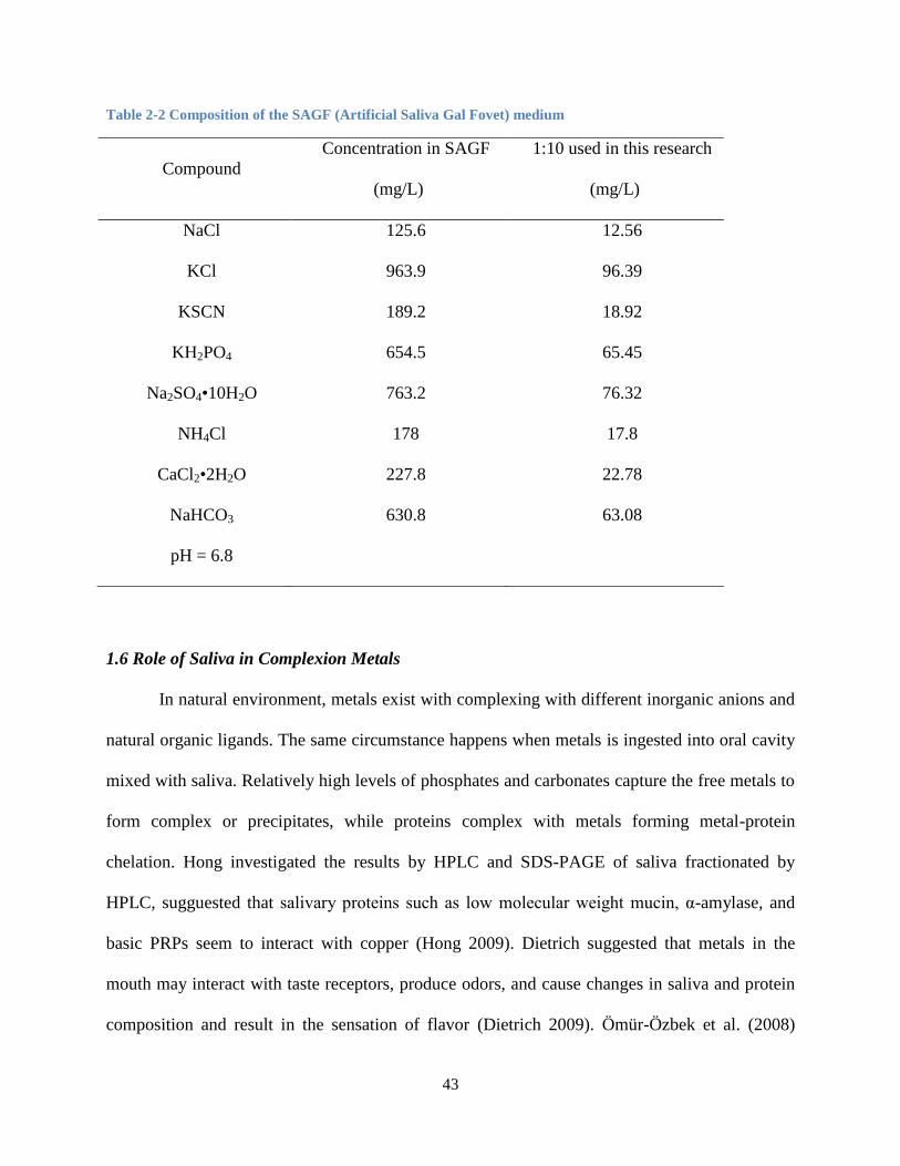
43
Table 2-2 Composition of the SAGF (Artificial Saliva Gal Fovet) medium
Compound
Concentration in SAGF
(mg/L)
1:10 used in this research
(mg/L)
NaCl 125.6 12.56
KCl 963.9 96.39
KSCN 189.2 18.92
KH2PO4 654.5 65.45
Na2SO4•10H2O 763.2 76.32
NH4Cl 178 17.8
CaCl2•2H2O 227.8 22.78
NaHCO3 630.8 63.08
pH = 6.8
1.6 Role of Saliva in Complexion Metals
In natural environment, metals exist with complexing with different inorganic anions and
natural organic ligands. The same circumstance happens when metals is ingested into oral cavity
mixed with saliva. Relatively high levels of phosphates and carbonates capture the free metals to
form complex or precipitates, while proteins complex with metals forming metal-protein
chelation. Hong investigated the results by HPLC and SDS-PAGE of saliva fractionated by
HPLC, sugguested that salivary proteins such as low molecular weight mucin, α-amylase, and
basic PRPs seem to interact with copper (Hong 2009). Dietrich suggested that metals in the
mouth may interact with taste receptors, produce odors, and cause changes in saliva and protein
composition and result in the sensation of flavor (Dietrich 2009). Ömür-Özbek et al. (2008)

44
demonstrated that copper (II) caused lipid oxidation, which is measured by the colorimetric
thiobarbituric acid reactive substances (TBARs) method, in the mouth at the presence of oxygen
(Omur-Ozbek 2008). Besides inducing lipid oxidation in the oral cavity, copper (II) also interacts
with salivary proteins and volatile odorants in the mouth to alter sensory perception (Hong et al.
2006, 2008). Epke et al. reported that nasal occlusion lowered the metallic taste and aftertaste
ratings of the two iron concentrations (0.001 M and 0.015 M) but the copper metallic taste and
aftertaste ratings were slightly influenced by nasal occlusion at the concentration of 0.001 M (64
mg/L) (Epke et al. 2009). Nasal occlusion increased thresholds for copper and iron when
retronasal sensations were eliminated (Epke et al. 2007). Those results suggested that nasal
perception plays an important role in the sensation of metallic flavor of iron but less important in
the sensation of copper, especially at high concentration of copper (II). Hong et al. (2006)
suggested that copper (II) interacted with the salivary proteins mucin and a-amylase at pH 7.5
but not pH 7 or 6.5 when added at 2.5 mg/l Cu to an artificial saliva consisting of salts and
proteins by detecting the headspace concentrations of hexanal, butyl acetate, 2-heptanone, and
ethyl hexanoate.
Hong et al. (2010) found that soluble copper species in a sample played a critical role in
perception of copper sensation by controlling metallic flavor, especially at the low copper levels.
Olivares et al. (2001) reported that copper imbibed in distilled water caused more gastrointestinal
distress than copper consumed in an orange-flavored beverage, which also indicated the
importance of free copper in the role of perception of copper.
Based on the lack on the role of free metals in generating metallic flavor, the goal of this
research is to:
Determine the role of free metals in the production of metallic flavor.

45
Predict chemical speciation of metals in artificial saliva in MINEQL+ and learn how free
metal ion concentration will vary with pH, protein content, other factors in oral cavity.
Compare predicted values with experimental results.

46
2. Materials and Methods
2.1 Artificial Saliva Solution Preparation
Distilled-deionized water was generated from a Barnstead Nanopure system that was fed
distilled water and subsequently deionized and carbon filtered. This system produced water with
a chemical resistivity of 18 MX/cm and pH 5.5.
Artificial saliva was prepared according to the following recipe, the inorganic components of
which coming from SAGF, while the organic components of which coming from Hong’s reports
(Hong et al. 2006). NaCl (0.1256 g), KCl (0.9639 g), KSCN (0.1892 g), KH2PO4 (0.6545 g),
Na2SO4 (0.3366 g), NH4Cl (0.178 g), CaCl2 (0.172 g) and NaHCO3 (0.6308 g) were separately
dissolved in 1000 ml nanopure water to make saliva stock solution. Both 0.216 g of mucin (from
porcine pancreas, Sigma, St. Louis, MO) and 20, 000 units of α-amylase (from Aspergillus
oryzae, Aldrich, Milwaukee, WI) were separately dispersed in two 100 mL of nanopure water to
make stock solutions of organic components. Nitric acid and sodium hydroxide were used to
adjust pH because of their weak affinity to copper. Artificial saliva solution was used for
experiments within one hour of preparation.

47
Table 2-3 Chemicals used in this research (1:10 dilution)
Compound Concentration(mg/L) Notes
NaCl 12.56
KCl 96.39
KSCN 18.92
KH2PO4 65.45
Na2SO4•10H2O 76.32 33.66mg/L as Na2SO4
NH4Cl 17.8
CaCl2•2H2O 22.78 17.2mg/L as CaCl2
NaHCO3 63.08
α-amylase (from
Aspergillus oryzae)
20 000 unit/L 37 units/mg
Mucin (from porcine
pancreas)
216 The molecular weight is not provided
by the manufacturer.
HNO3 - Used to adjust pH
NaOH - Used to adjust pH
2.2 Treatment of copper
A 1000 mg/l copper stock solution was prepared from copper (II) sulfate pentahydrate
(catalog number C493-500, Fisher Scientific, Pittsburgh, PA, USA) and diluted to obtain
concentrations in the range of 0.1-10 mg/l Cu. All samples were prepared fresh daily to avoid
increased precipitation with time and loss of carbonate. All copper solutions were prepared and
maintained at room temperature, within 22-24C.

48
When water is ingested into oral cavity, saliva is diluted by the water consumed. Therefore we
must consider the influence of dilution on the chemical speciation of copper in oral cavity.
Considering the regular amount of water uptake and the saliva volume, we chose 1:10 (saliva:
water) as our dilution rate. In order to investigate the contribution of inorganic components and
proteins, total copper concentration and pH on the chemical speciation of copper, we designed
our experiments in Table 2-4. We measured the free copper in the five combinations under three
kind of copper treatment (2.5mg/L (0.04 mM), 5mg/L (0.08 mM), 10 mg/L (0.16 mM)), under
five different pH (5.5, 6, 6.5, 7, 7.5).
Table 2-4 Experimental design table
Components Copper concentration (mg/L)
Only Inorganic 2.5 5 10
Inorganic and α-amylase 2.5 5 10
Only α-amylase 2.5 5 10
Inorganic and mucin 2.5 5 10
Only mucin 2.5 5 10
2.3 Ion Selective Electrode measurement
Among the many analytical methods available for determining copper in aquatic environments,
only potentiometry with copper ion-selective electrodes (ISEs) can directly measure the free
copper ion in situ without perturbing the natural speciation (Belli and Zirino 1993). Free copper
ion concentrations were measured using a cupric electrode (Accumet cupric combination
electrode, catalog number 13-620-547, Fisher Scientific).

49
The cupric electrode membrane is composed of sulfides of copper and other metals bonded
into a glass body. When the electrode is in contact with free, unbound cupric ions in solution, a
potential develops across the membrane, which vary with concentration in a Nernstian fashion:
E = E0
+ 2.3 (RT/nF) log [Cu2+
]
where
E is the mV potential from the electrode
E0 is the sum of all other constant system potentials
R is the gas constant
T is the temperature in degrees Kelvin
n is the number of electrodes required to reduce Cu2+
F is Faraday’s constant
The electrode has a range of detection 1×10⁻¹
to 1×10⁻⁸
M Cu2+
and works in the pH range of
2-12 and temperature range of 0 to 80˚C. Sodium nitrate is a non-complexing component and
was used to adjust ionic strength. 5M NaNO3 is used as Ionic Strength Adjuster (ISA). When
measuring the samples, 2 ml ISA was added into 100 ml sample mixed well with a Thermix
Stirrer (Fisher Scientific). All free copper ISE measurements were made within 5 minutes of
adding copper to saliva.
2.4 Modeling Metal Speciation
In order to compare with our experimental data with predicted results, the concentrations
of soluble and precipitated copper in the artificial saliva model systems were estimated by
MINEQL+ chemical equilibrium modeling software (version 4, Environmental Research
Software, Hallowell, ME). The soluble copper concentration in the artificial saliva model system

50
with protein could not be calculated by the MINEQL+ software because thermodynamic data of
salivary proteins-electrolytes interaction required for calculation are not available.
3. Results and Discussion
3.1 Predicting Speciation of Cu, Fe and Zn with Inorganic Components of Saliva
Soluble free metal ion concentrations in MINEQL+ models for cu, Fe and Zn
Free metals concentrations including copper, ferrous and zinc in diluted SAGF medium
were modeled in MINEQL+ at different pH values and displayed in Figure 2-4-a. Dilution rate
was 1:10 in all samples assuming that average about 10 ml per drink for normal people and
average volume in the mouth of 1.1 ml (Llena-Puy 2006). All the samples were treated with
sulfate (CuSO4, FeSO4 and ZnSO4) with 10 mg/L as metal ion. Closed to atmosphere, which is
an option in the software, was applied in MINEQL+ because all the samples were prepared and
measured in a short time.
All of the free metal concentrations changed with pH in a similar trend, decreasing as pH
increased from 5.5 to 7.5 and tending to zero after 7.5. In the range of 6.5 to 7.5, the typical pH
of human saliva (Dietrich 2009), free metal concentrations only are a small part of the total metal
(less than 5%), indicating that most of the metals are combined with inorganic components in
saliva in the absence of proteins. Comparing Figure 2-4-a and Figure 2-4-b, which shows the free
metals in distilled-deionized water at different pH, chemical speciation of metals in water
significantly changed after ingested into the oral cavity. The notable decrease in free form of
metals would reduce the bioavailability of them in the oral cavity, especially for ferrous and zinc.
In other words, the impact of saliva components on ingested aqueous metals must be considered

51
in order to understand the mechanism of metallic flavor and the fate of metals in the human
mouth.
Figure 2-4 Free metal ion concentration as a function of pH modeled by MINEQL+; a: inorganic components
of artificial saliva; b: nanopure water; total metal concentration was 10 mg/L as metal.
Soluble and Insoluble Metal Complexes
Metals exist in free, soluble complexes and precipitates in aqueous environment as well
as in human saliva. Free, soluble complexes and precipitate forms of metals in artificial saliva
0
1
2
3
4
5
6
7
8
9
10
5 5.5 6 6.5 7 7.5 8
Fre
e m
eta
l co
nce
ntr
atio
n (
mg/
L)
Cu2+
Fe2+
Zn2+
0
1
2
3
4
5
6
7
8
9
10
5 5.5 6 6.5 7 7.5 8
Fre
e m
eta
l co
nce
ntr
atio
n m
g/L
pH
Cu2+
Fe2+
Zn2+
b
a

52
with only inorganic components were modeled and presented in Figure 2-5. Free ion
concentration decreased and precipitates increased with the increasing of pH from 5.5 to 7.5, for
all the three metals. At pH 5.5, about 50% of the metals are in the free form and at pH of 7 and
above, free ion concentrations dropped to nil. There is a small portion of metals in soluble
complexes at low pH, but this proportion decreases as pH rises. The trend is similar to the
situation of copper in nanopure water in Figure 2-4. Compared with copper and iron, zinc has
less solubility in artificial saliva at pH 5.5.

53
Figure 2-5 Distribution of free, soluble and precipitate forms of metals in inorganic artificial saliva at various
pH values; A: Copper (Cu2+
); B: Iron (Fe2+
); C: Zinc (Zn2+
)
Table 2-5 demonstrates the chemical speciation of 10 mg/L of metals in inorganic
artificial saliva including the species of precipitates. Cupric phosphate, malachite and tenorite are
the three major precipitates; therefore, PO43-
, OH- and CO3
2- have high affinity for copper. Their
percentages in total precipitates vary with pH because pH controls the species distribution of
phosphate and carbonate. The proportion of total soluble has the reverse trend with precipitate,
0%
20%
40%
60%
80%
100%
5.5 6 6.5 7 7.5
0%
20%
40%
60%
80%
100%
5.5 6 6.5 7 7.5
0%
20%
40%
60%
80%
100%
5.5 6 6.5 7 7.5Precipitate Soluble FreeC
A
B
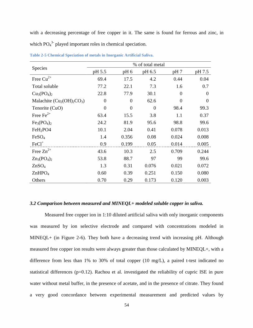
54
with a decreasing percentage of free copper in it. The same is found for ferrous and zinc, in
which PO43-
played important roles in chemical speciation.
Table 2-5 Chemical Speciation of metals in Inorganic Artificial Saliva.
Species % of total metal
pH 5.5 pH 6 pH 6.5 pH 7 pH 7.5
Free Cu2+
69.4 17.5 4.2 0.44 0.04
Total soluble 77.2 22.1 7.3 1.6 0.7
Cu3(PO4)2 22.8 77.9 30.1 0 0
Malachite (Cu2(OH)2CO3) 0 0 62.6 0 0
Tenorite (CuO) 0 0 0 98.4 99.3
Free Fe2+
63.4 15.5 3.8 1.1 0.37
Fe3(PO4)2 24.2 81.9 95.6 98.8 99.6
FeH2PO4 10.1 2.04 0.41 0.078 0.013
FeSO4 1.4 0.356 0.08 0.024 0.008
FeCl+ 0.9 0.199 0.05 0.014 0.005
Free Zn2+
43.6 10.3 2.5 0.709 0.244
Zn3(PO4)2 53.8 88.7 97 99 99.6
ZnSO4 1.3 0.31 0.076 0.021 0.072
ZnHPO4 0.60 0.39 0.251 0.150 0.080
Others 0.70 0.29 0.173 0.120 0.003
3.2 Comparison between measured and MINEQL+ modeled soluble copper in saliva.
Measured free copper ion in 1:10 diluted artificial saliva with only inorganic components
was measured by ion selective electrode and compared with concentrations modeled in
MINEQL+ (in Figure 2-6). They both have a decreasing trend with increasing pH. Although
measured free copper ion results were always greater than those calculated by MINEQL+, with a
difference from less than 1% to 30% of total copper (10 mg/L), a paired t-test indicated no
statistical differences (p=0.12). Rachou et al. investigated the reliability of cupric ISE in pure
water without metal buffer, in the presence of acetate, and in the presence of citrate. They found
a very good concordance between experimental measurement and predicted values by
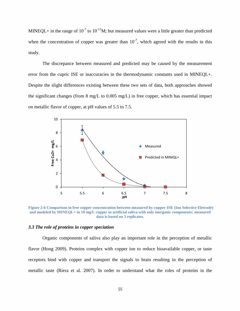
55
MINEQL+ in the range of 10-7
to 10-12
M; but measured values were a little greater than predicted
when the concentration of copper was greater than 10-7
, which agreed with the results in this
study.
The discrepance between measured and predicted may be caused by the measurement
error from the cupric ISE or inaccuracies in the thermodynamic constants used in MINEQL+.
Despite the slight differences existing between these two sets of data, both approaches showed
the significant changes (from 8 mg/L to 0.005 mg/L) in free copper, which has essential impact
on metallic flavor of copper, at pH values of 5.5 to 7.5.
Figure 2-6 Comparison in free copper concentration between measured by copper-ISE (Ion Selective Eletrode)
and modeled by MINEQL+ in 10 mg/L copper in artificial saliva with only inorganic components; measured
data is based on 3 replicates.
3.3 The role of proteins in copper speciation
Organic components of saliva also play an important role in the perception of metallic
flavor (Hong 2009). Proteins complex with copper ion to reduce bioavailable copper, or taste
receptors bind with copper and transport the signals to brain resulting in the perception of
metallic taste (Riera et al. 2007). In order to understand what the roles of proteins in the
0
2
4
6
8
10
5 5.5 6 6.5 7 7.5 8
Fre
e C
u2
+ m
g/L
pH
Measured
Predicted in MINIQL+

56
perception of metallic taste and how they impact the free copper concentration in oral cavity,
three major proteins of human saliva- α-amylase, mucin and lactoferrin - were studied in this
section.
Due to the lack of available constants for proteins, MINEQL+ cannot be used to model the
environments containing organic compounds.
α-amylase
Free copper concentrations in the samples with only inorganic components, α-amylase
plus inorganic components and only α-amylase at three different copper treatments were
demonstrated in Figure 2-7. The different plots illustrate the results in samples treated with
different concentrations of copper. The concentration of α-amylase in all the samples is 200, 000
unit/L (5.38 g/L) (Hong et al. 2006).
α-amylase significantly impacted the free copper concentration at low pH in small
concentration of total copper. With the increase of total copper from 2.5 mg/L to 10 mg/L, the
influence of α-amylase in chemical speciation of copper declined gradually. At pH of 6.5, α-
amylase tended to increase the free copper concentration, compared with that in saliva with only
inorganic components. These results suggested that α-amylase has limited binding capacity with
copper; it controlled the chemical speciation of copper at low concentration of copper, but when
more copper exists in the samples, the chemical distribution of the excess portion of copper
beyond the capacity of α-amylase is still controlled by the inorganic components. Compared with
its high content in human saliva, where 40% to 50% of the total salivary gland-produced protein
is α-amylase (Tenovuo 1989), the influence of α-amylase on chemical speciation of copper is
slight.
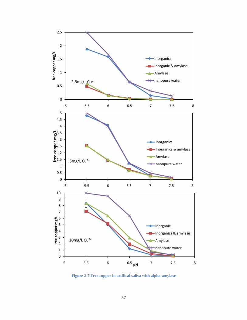
57
Figure 2-7 Free copper in artifical saliva with alpha-amylase
0
0.5
1
1.5
2
2.5
5 5.5 6 6.5 7 7.5 8
fre
e c
op
pe
r m
g/L
Inorganics
Inorganic & amylase
Amylase
nanopure water2.5mg/L Cu2+
0
0.5
1
1.5
2
2.5
3
3.5
4
4.5
5
5 5.5 6 6.5 7 7.5 8
fre
e c
op
pe
r m
g/L
Inorganics
Inorganics & amylase
Amylase
nanopure water5mg/L Cu2+
0
1
2
3
4
5
6
7
8
9
10
5 5.5 6 6.5 7 7.5 8
Fre
e c
op
pe
r m
g/L
pH
Inorganic
Inorganics & amylase
Amylase
nanopure water
10mg/L Cu2+

58
Mucin
Mucin is another major component of human saliva. Mucins, high-molecular-weight
glycoproteins account for 7-26% of total salivary proteins (Slomiany, Murty et al. 1996). The
same experimental and analytical method was used for mucin to investigate its effects on the
chemical speciation of copper in diluted artificial saliva. Figure 2-8 demonstrated the comparison
in free copper among three kind of artificial saliva in three different concentrations of total
copper. Only a small amount of copper (less than 5% of total copper) was in free form at the
existence of mucin, no matter what the total concentration of copper and the pH was. This
suggested that mucin had very high affinity to copper in the given mucin concentration (2.16 g/L)
and pH range, which was consist with Mueller’s results: binding of copper to glycoprotein was
as high as 5.0M Cu/M protein (Mueller 1983). Although free ion concentrations in artificial
saliva with mucin were at low levels, a decreasing tendency could be found with the increase of
pH in all samples.

59
Figure 2-8 Free copper in artificial saliva with mucin
Due to the high binding capacity between copper and mucin, it is difficult to find out the
influence of mucin on copper speciation at different pH. Therefore, experiments were repeated in
0
0.5
1
1.5
2
2.5
5 5.5 6 6.5 7 7.5 8
fre
e c
op
pe
r m
g/L
pH
Inorganics
Inorganics & Mucin
Mucin
nanopure water
0
0.5
1
1.5
2
2.5
3
3.5
4
4.5
5
5 5.5 6 6.5 7 7.5 8
fre
e c
op
pe
r m
g/L
pH
Inorganics
Inorganics & Mucin
Mucin
nanopure water
0
1
2
3
4
5
6
7
8
9
10
5 5.5 6 6.5 7 7.5 8
fre
e c
op
pe
r m
g/L
pH
Inorganics
Inorganics & Mucin
Mucin
nanopure water
10mg/L Cu2+

60
saliva with diluted mucin. Figure 2-9 showed the results of free copper in artificial saliva with
different concentrations of mucin at total copper of 10 mg/L. The free ion concentrations were
significantly influenced by the levels of mucin in artificial saliva, especially at low pH. With the
increase of mucin from 10% to 100%, the free ions dropped gradually at each pH. However, the
line without mucin is not totally above the lines with mucin on the graph, which meant mucin
could increase the free copper level at certain concentrations of mucin and certain pH, such as 10%
of mucin at pH of 6. This may be due to the interaction between mucin and other inorganic
components those also complex with copper. This result could be one of the explanations for the
various threshold values among individuals because different people have different pH and
concentrations of mucin, and these factors could results in various levels of free copper.
Figure 2-9 The impacts of mucin concentration on the free copper concentration in artificial saliva
Lactoferrin
Lactoferrin consists of two domains that each bind one Fe3+
reversibly but tightly (K =
1020
). It was also found to accommodate other transition metal ions such as Cr3+
, Mn3+
, Al3+
,
Co3+
, Cu2+
, and Zn2+
with less binding affinity than that to Fe3+
. The binding between lactoferrin
0
0.5
1
1.5
2
2.5
3
3.5
4
5 5.5 6 6.5 7 7.5 8
Fre
e C
U2
+ m
g/L
pH
inorganics+0%mucin
inorganics+10%mucin
inorganics+50%mucin
inorganics+70%mucin
inorganics+100%mucin
Note: 1. 100%mucin is 2.16g/L2. 10mg/L of copper

61
and other metal ions would change the structure of lactoferrin and impacts its binding ability to
ferric ion (Baker, Anderson et al. 1990). Although this suggests the possibility of copper-
lactoferrin interaction, there has been no previous study on lactoferrin-copper binding in human
saliva.
This section mainly studied the binding capacity of lactoferrin to copper and investigate its
effects on the perception of metallic flavor of copper. The same experiment plan was designed
like α-amylase and mucin as discussed above. By comparing the free copper in artificial saliva
with and without lactoferrin, the slight changes between the sets of data in figure 12 suggested
that there was some interaction between copper and lactoferrin but the binding capacity between
them is very weak at a concentration of 1 mg/L of lactoferrin concentration.
Figure 2-10 The impacts of lactoferrin on the free copper concentration in artificial saliva; data points
represent mean of triplicate measurement; error bars are shown but are not visible
0
1
2
3
4
5
6
7
8
9
10
5 5.5 6 6.5 7 7.5 8
Fre
e C
u2
+
mg
/L
pH
Inorganics
inorganics & Lactoferrin
Only Lactoferrin
Note:
1. C(Lac)=1ug/ml=1mg/L
2. 1:10 dilution
3. C(Cu2+)= 10mg/L

62
3.4 Binding capacity of proteins with copper
Figure 2-8 and 2-9 demonstrated the influence of amylase and mucin on the free copper
concentration, while Table 2-5 shows the approximate binding capacity of these two proteins to
copper at different pH. The binding capacity was calculated by the following equation,
Binding capacity (mg Cu/g protein) = (Ct-Cw-Cp)/Mp
where
Ct is the total concentration of copper;
Cw is the non-free copper concentration in the nanopure water with corresponding total
concentration of copper, so Ct-Cw represented the available copper to bind protein;
Cp is the free copper concentration in the artificial saliva with only protein;
Mp is the protein concentration.
This estimation ignored the interaction between proteins and other inorganic or organic
components in saliva and provided us the approximate information on the copper-protein binding
capacity. At pH of 5.5, the binding capacity of amylase to copper did not change too much with
various copper concentrations but at higher pH there was significant difference in different
copper concentrations. Amylase showed the strongest binding capacity to copper at pH of 6.5
and copper concentration of 10 mg/L, which suggested that pH and total metal concentration
both influenced the interaction between amylase and copper.
Mucin generally had greater (about 10 times) binding capacity with copper than amylase
from Table 2-6. With the decrease of total copper concentration and the increase of pH, the
binding capacity dropped gradually. The maximum point was at total copper concentration of 10
and pH of 5.5, indicating that mucin may have greater binding capacity with copper at higher
copper concentration and lower pH.

63
Table 2-6 Binding capacity of amylase and mucin to copper at different pH
Binding capacity (mg Cu/g protein)
Cu2+
(mg/L) pH=5.5 pH=6 pH=6.5 pH=7
Amylase 2.5 3.53 2.84 1.14 0.58
5 4.59 4.65 1.02 0.39
10 2.99 5.74 6.47 0
Mucin 2.5 10.29 7.62 2.98 1.47
5 22.33 18.34 5.63 2.19
10 43.58 43.48 29.58 3.24 Each data point represents a mean for triplicate measurements; the coefficient of variation was less than 5% for all
triplicates
3.5 Changes of pH and free copper in saliva with time.
Considering the kinetic aspects of the reaction between copper and saliva components,
the changes of free copper with time in inorganic saliva was studied in this section. Figure 2-11
clearly showed the descending trend in free copper with time; this may imply the kinetic
transforming of copper species in artificial saliva, resulting in the changes in free copper as well
as other species of copper. This accords with Dietrich et al.’s finding that formation of malachite
was observed within 3 min after initiating a reaction, but reached equilibrium after 96 h (Dietrich
et al. 2005). This also seems to be able to explain the difference between experimental data and
predicted data in MINEQL+, which models the environment in equilibrium. However, the pH of
the sample also changed with time, which was shown in Figure 2-11. The increase of pH could
not be due to the reaction of forming precipitates, because all the processes of precipitate
formation of malachite, copper phosphate and tenorite generate H+ and reduce the pH. One
possible reason of the increase in pH and decrease in free copper was the diffusion of carbon
dioxide from artificial saliva to the air.

64
Figure 2-11 Changes in free copper concentration and pH of inorganic artificial saliva with time in 2.5 mg/L
of total copper
6.5
6.6
6.7
6.8
6.9
7
7.1
7.2
7.3
7.4
7.5
0
0.1
0.2
0.3
0.4
0.5
0.6
0 50 100 150 200
pH
Cu
2+
time/min
Cu2+

65
4. Conclusions and Suggestions
Chemical speciations of copper, iron and zinc were modeled by MINEQL+ and main
species including the free portion and precipitates were analyzed and compared at different pH.
By comparing experimental data with predicted data in MINEQL+, the practicability and
limitation of cupric ISE and MINEQL+ used in understanding the chemical speciation of metals
in saliva were investigated. Although the two methods were not accurate enough to reflect the
real situation perfectly, we can still use them to know the probable concentrations of each species
and trends of those species varying with pH, concentration of saliva components and time.
Inorganic components, typically phosphate, carbonate and hydroxide combined with copper and
greatly controlled the levels of free copper when water was ingested in oral cavity. Proteins such
as α-amylase, mucin and lactoferrin also impacted the chemical speciation of copper. In the three
major proteins studied, mucin had the greatest affinity with copper, followed by α-amylase, and
lactoferrin had very weak binding capacity with copper at the concentrations considered in this
study. Inorganic components dominated in the chemical speciation of copper when no levels of
mucin existed in artificial saliva. When the concentration of mucin was raised to 0.216 g/L
(approximately 10% of total mucin in saliva), free copper is controlled by the concentration of
mucin. The monitoring of free copper with time was conducted to study the kinetic processes
that happen when copper was ingested into oral cavity. Free copper decreased with time but pH
also increased at the meantime, which made it difficult to explain what caused the reducing of
free copper: pH or the chemical reactions involving copper.
5. Reference
Allen, L. a. S., J.C. (2001). Prevalence of nutritional anaemia. Nutritional Anaemia (U.
Ramakrishnan, ed.): 39-49.

66
Baker, E. N., B. F. Anderson, et al. (1990). Metal and anion binding sites in lactoferrin and
related proteins. Pure and Applied Chemistry 62(6): 1067-1070.
Beguinbruhin, Y., F. Escher, et al. (1983). Threshold concentration of copper in drinking-water.
Lebensmittel-Wissenschaft & Technologie 16(1): 22-26.
Belli, S. L. and A. Zirino (1993). Behavior and Calibration of the Copper( I I) Ion-Selective
Electrode in High Chloride Media and Marine Waters. Analytical Chemistry 65(19): 2583-
2589.
Borocz-Szabo, M. (1980). The influence of iron contamination on the sensory properties of
liquid foods. Acta Alimentaria 9: 341–356.
Breslin, P. A. S., M. M. Gilmore, et al. (1993). Psychophysical evidence that oral astringency is a
tactile sensation. Chemical Senses 18(4): 405-417.
Brezonik, P. L., S. O. King, et al. (1991). The influence of water chemistry on trace metal
bioavailability and toxicity to aquatic organisms. Metal Ecotoxicology: Concepts and
Applications.
Cavdar, A. O. (2000). Analysis of zinc (serum, plasma erythrocyte, and hair zinc) and its relation
to nutrition in pregnant Turkish women:Areview of cross-sectional and longitudinal studies. J.
Trace Elem. Exp. Med. 13: 63–71.
Cohen, J., J. Kamphake, et al. (1960). Taste threshold concentrations of metals in drinking water.
J. Am.Water Works Assoc. 52: 660-670.
Cuppett, J. D., S. E. Duncan, et al. (2006). Evaluation of copper speciation and water quality
factors that affect aqueous copper tasting response. Chemical Senses 31(7): 689-697.
Dameron, C. H., P.D. (1998). Environmental health criteria for copper. Environmental health
criteria 200: Available from http://www.inchem.org/documents/ehc/ehc/ehc200.htm#Section
Number:201.203.
Dawes, C. (1987). Physiological factors affecting salivary flow-rate, oral sugar clearance and the
sensation of dry mouth in man. Journal of Dental Research 66: 648-653.

67
Demaeyer, E. a. A.-T., M. (1985). The prevalence of anaemia in the world. World Health Stat.
38: 302–316.
Dietrich, A., J. Cuppett, et al. (2005). Corrosion of copper plumbing and its effects on consumer
health and economics. In NSF design, manufacture, and industrial innovation (DMII) grantee
conference . Scottsdale, AZ: National Science Foundation. : pp. 1-14.
Dietrich, A. M. (2009). The sense of smell: contributions of orthonasal and retronasal perception
applied to metallic flavor of drinking water. Journal of Water Supply Research and
Technology-Aqua 58(8): 562-570.
Dietrich, A. M., D. Glindemann, et al. (2004). Health and aesthetic impacts of copper corrosion
on drinking water. Water Science and Technology 49(2): 55-62.
Epke, E. M., Lawless, H. T. (2007). Retronasal smell and detection thresholds of iron, copper
and sodium salts. Physiology and Behavior 92: 487–491.
Epke, E. M., S. T. McClure, et al. (2009). Effects of nasal occlusion and oral contact on
perception of metallic taste from metal salts. Food Quality and Preference 20(2): 133-137.
EWR (2005). Copper. National tap water quality database. <http://www.ewg.org/tapwater/
contaminants/contaminant.php?contamcode=1022>.
Griffith, D. P., D. A. Liff, et al. (2009). Acquired Copper Deficiency: A Potentially Serious and
Preventable Complication Following Gastric Bypass Surgery. Obesity 17(4): 827-831.
Hambidge, K. M. a. K., N. F. (2007). Zinc deficiency: a special challenge. J. Nutr. 137(4): 1101.
Hercberg, S., Galan, P. and Dupin, H. (1987). Iron deficiency in Africa. World Rev. Nutr. Diet
54: 201–236.
Hong, J., Susan E. Duncan, Andrea M. Dietrich, Sean F. O’Keefe, William N. Eigel, and Kumar
Mallikarjunan. (2009). Interaction of Copper and Human Salivary Proteins. Journal of
Agricultural and Food Chemistry 57(15): 6967–6975.

68
Hong, J. H., S. E. Duncan, et al. (2010). Effect of copper speciation at different pH on temporal
sensory attributes of copper. Food Quality and Preference 21(1): 132-139.
Hong, J. H., S. E. Duncan, et al. (2006). Effect of copper on the volatility of aroma compounds
in a model mouth system. Journal of Agricultural and Food Chemistry 54(24): 9168-9175.
Hong JH, S. E. D., Andrea M. Dietrich, Sean F. O’Keefe, William N. Eigel, and Kumar
Mallikarjunan. (2009). Interaction of Copper and Human Salivary Proteins. Journal of
Agricultural and Food Chemistry 57(15): 6967–6975.
Hurrell, R. (1985). Nonelemental sources. In: Clydesdale FM, Wiemer KL, editors. Iron
fortification of foods. Orlando, Fla.: Academic Press. 39–41.
Jensen, J. N. (2003). A problem-solving approach to aquatic chemistry; Hoboken: Wiley
& Sons, Inc..
Jensen, J. N. (2003). A problem - solving approuch to Aquatic Chemistry. 562-563.
Keast, R. S. J. (2003). The effect of zinc on human taste perception. Journal of Food Science
68(5): 1871-1877.
Knobeloch, L., M. Ziarnik, et al. (1994). Gastrointestinal upsets associated with ingestion of
copper-contaminated water. Environmental Health Perspectives 102(11): 958-961.
Lawless, H. T., S. Schlake, et al. (2004). Metallic taste and retronasal smell. Chemical Senses
29(1): 25-33.
Lawless, H. T., D. A. Stevens, et al. (2005). Metallic taste from electrical and chemical
stimulation. Chemical Senses 30(3): 185-194.
Lim, J. and H. T. Lawless (2006). Detection thresholds and taste qualities of iron salts. Food
Quality and Preference 17(6): 513-521.
Litovitz, T. L., B. F. Schmitz, et al. (1989). 1988 Annual-report of the american-association –of
poison-control-centers national data-collection system. American Journal of Emergency
Medicine 7(5): 495-544.

69
Llena-Puy, C. (2006). The rôle of saliva in maintaining oral health and as an aid to diagnosis.
Med Oral Patol Oral Cir Bucal 11: E449-E455.
Lozoff, B., Jimenez, E. and Xolf, A.W. (1991). Long term development outcome of infants with
iron deficiency. N. Engl. J. Med. 325: 687–694.
Meador, J. P. (1991). The interaction of pH, dissolved organic-carbon, and total copper in the
determination of ionic copper and toxicity. Aquatic Toxicology 19(1): 13-31.
Moretti, D., T. C. Lee, et al. (2005). Development and evaluation of iron-fortified extruded rice
grains. Journal of Food Science 70(5): S330-S336.
Mueller, H. J. (1983). The binding of corroded methallic-ions to salivary-type proteins.
Biomaterials 4(2): 66-72.
NRC (2000). copper in drinking water.
Olivares, M., M. Araya, et al. (2001). Nausea threshold in apparently healthy individuals who
drink fluids containing graded concentrations of copper. Regulatory Toxicology and
Pharmacology 33(3): 271-275.
Omur-Ozbek, P., Dietrich, A. M., Duncan, S. E. & Lee, Y.-W. (2008). Metallic flavor of iron
and copper in drinking water,presented at the IWA 8th International Symposium on Off-
Flavours in the Aquatic Environment, October 2008 Seoul, Korea.
Pangborn, R. M. and B. Lundgren (1977). Salivary secretion in response to mastication of crisp
bread. Journal of Texture Studies 8(4): 463-472.
Patnaik, P. (2002). Handbook of Inorganic Chemicals. McGraw-Hill. ISBN 0070494398.
Pizarro, F., M. Olivares, et al. (1999). Acute gastrointestinal effects of graded levels of copper in
drinking water. Environmental Health Perspectives 107(2): 117-121.
Prasad, A. S. (2003). Zinc deficiency. British Medical Journal 326(7386): 409.

70
Rachou, J., C. Gagnon, et al. (2007). Use of an ion-selective electrode for free copper
measurements in low salinity and low ionic strength matrices. Environmental Chemistry 4(2):
90-97.
Riera, C. E., H. Vogel, et al. (2007). Artificial sweeteners and salts producing a metallic taste
sensation activate TRPV1 receptors. American Journal of Physiology-Regulatory Integrative
and Comparative Physiology 293(2): R626-R634.
Roeser, H. P. (1986). Iron. J. Food Nutr.,(42): 82–92.
Sanstead, H. H. (1995). Is zinc deficiency a public health problem? Nutrition 11: 87–92.
Scrimshaw, N. S. (1984). Functional consequences of iron deficiency in human populations. J.
Nutr. Sci. Vitaminol. 30: 47–63.
Slomiany, B. L., V. L. N. Murty, et al. (1996). Salivary mucins in oral mucosal defense. General
Pharmacology 27(5): 761-771.
Snoeyink, V. L. and D. Jenkins (1980). Water Chemistry. John Wiley and Sons, Inc., New York,
NY, USA. .
Snoeyink, V. L. and D. Jenkins (1980). Water Chemistry. 249-249.
Suffet, I. H., J. Mallevialle, et al. (1995). Advances in Teste-and-Odor Treatment and Control
AWWARF, Lyonnaise des Eaux-Dumes, Denver, CO.
Swanson, C. A. a. K., J.C. (1987). Zinc and pregnancy outcome. Am. J. Clin. Nutr. 46: 763–771.
Symes, J. L. and D. R. Kester (1984). THERMODYNAMIC STABILITY STUDIES OF THE
BASIC COPPER CARBONATE MINERAL, MALACHITE. Geochimica Et Cosmochimica
Acta 48(11): 2219-2229.
Tenenbein, M. (2005). Unit-Dose Packaging of Iron Supplements and Reduction of Iron
Poisoning in Young Children. Arch Pediatr Adolesc Med. 159: 557-560.
Tenovuo, J. O. (1989). Human Saliva: Clinecal Chemistry and microbiology. Volume II: 107-
107.

71
USEPA (1991). Maximum contaminant level goals and national primary drinking water
regulations for lead and copper;final rule. Federal Register 56(110): 26460-26564.
USEPA (2009). List of National Secondary Drinking Water Regulations.
Valder-Ramos, R. (1992). Zinc:Aperinatal point of view. Food Nutr. Sci. 16: 279–306.
WHO (1998). World Health Organization Guidelines for Drinking Water Quality. 2nd edn,
Addendum to vol. 2. Health Criteria and Other SupportingInformation.
WHO (2007). The impact of zinc supplementation on childhood mortality and severe morbidity,
World Health Organization.
Wisniewski, L., L. H. Epstein, et al. (1992). Effect of food change on consumption, hedonics and
salivation. Physiology & Behavior 52(1): 21-26.
Wu, A. M., G. Csako, et al. (1994). Structure, biosynthesis, and function of salivary mucins.
Molecular and Cellular Biochemistry 137(1): 39-55.
Young, J. A. and C. A. Schneyer (1981). Composition of saliva in Mammalia. Australian Journal
of Experimental Biology and Medical Science 59(FEB): 1-53.
Zacarias, I., C. G. Yanez, et al. (2001). Determination of the taste threshold of copper in water.
Chemical Senses 26(1): 85-89.

72
Appendix
Abbreviation
PE Polyethylene
NOM Natural Organic Matter
PEX Cross-linked polyethylene
HDPE High density polyethylene
OIT Oxidation induction time
Kow Octanol water partition coefficient
MTBE Methyl tert-butyl ether
Sw Water solubility
Mv Molecular volume
Vocs Volatile organic compounds
ISE Ion selective electrode
SDS-PAGE Sodium dodecyl sulfate polyacrylamide gel electropheresis
SAGF Artificial Saliva Gal Fovet
HPLC High Performance Liquid Chromatography
TBARS Thiobarbituric Acid Reactive Substances

73
Data for regression model
Appendix A-1 Contaminant Characteristics at 25 ºC
Contaminant Name
Contaminant Property
μ,
Debye
Mm,
g/mol
ρ,
g/cm3
Mv,
cm3
Sw,
mg/L
Log
Kow
Polar Contaminants
Acetonitrile 3.92 41.05 0.786 53.3 Miscible –0.34
2–Propanone 2.88 58.08 0.789 73.1 Miscible –0.24
Benzaldehyde 2.80 106.12 1.041 120.5 3000 1.48
2–Butanone 2.76 72.11 0.805 91.4 223000 0.29
Water 1.85 18.01 1.000 19.1 Miscible –
Benzyl Alcohol 1.71 108.14 1.041 125.1 40000 1.10
1–Butanol 1.66 74.12 0.809 96.2 74000 –0.30
2–Propanol 1.56 60.10 0.789 77.8 Miscible 0.05
Nonpolar Contaminants
Dichloromethane 1.60 84.93 1.326 60.6 13030 1.25
Methyl t–butyl ether 1.36 88.15 0.740 119.1 51000 1.24
Trichloromethane 1.01 119.37 1.492 74.4 7290 1.97
Toluene 0.36 92.14 0.867 117.7 526 2.73
m–Xylene 0.30 106.16 0.864 135.9 161 3.20
p–Xylene 0.00 106.16 0.867 135.8 162 3.15
μ = Dipole moment; δ = Solubility parameter; Mv = Molar volume; Mm = Molar mass; Sw = Water solubility; ρ = Density; Kow =
Octanol–water partition coefficient; Mm, Sw, Log Kow, and ρ values obtained from CHEMFATE (Syracuse Research Corporation
2009).

74
Appendix A-2 Bulk Characteristics of Polyethylene Materials
Property
Type of Polyethylene1
HDPE
Resin
Monomodal
HDPE
Pipe
Bimodal
HDPE
Pipe
PEX–A
Pipe
(MDPE)
PEX–B1
Pipe
(HDPE)
PEX–B2
Pipe
(HDPE)
Thickness, mm. 1.65 + 0.02 2.61 + 0.05 2.59 + 0.08 2.60 + 0.02 2.64 + 0.03 2.63 + 0.03
Composition
Polymer 99.9% 97.8% 97.7% 99.8% 99.4% 99.4%
Char & Carbon Black 0% 2.1% 2.0% 0% 0.1% 0.1%
Volatile Loss at 150 ºC 0.1% 0.1% 0.2% 0.2% 0.5% 0.5%
Ash 0% 0% 0.1% 0% 0% 0%
Oxidative Resistance and Morphology
Tdegonset, ºC 431 459 465 460 462 461
Tdeg, ºC 465 479 485 482 484 484
Tmonset, ºC 127.0 + 0.6 121.7 + 0.2 123.4 + 0.5 120.3 + 1.2 119.8 + 1.1 119.5 + 0.6
Tm, ºC 135.1 + 0.5 128.7 + 0.5 130.2 + 0.1 130.1 + 0.4 130.0 + 0.3 129.7 + 0.2
OIT (min.) 22.4 + 2.4 92.5 + 1.3 119.6 + 1.1 33.6 + 3.9 119.6 + 12.3 > 295
Bulk Density, g/cm3
0.9572 +
0.0001
0.9494 +
0.0002 0.9547 + 0.0001 0.9371 + 0.0005 0.9524 + 0.0001
0.9510 +
0.0001
Crystallinity
by Tm, % 62.7 + 0.6 50.9 + 1.9 51.7 + 2.4 45.4 + 2.1 54.4 + 2.7 54.9 + 1.1
by Density, % 74.3 + 0.1 69.3 + 0.1 72.7 + 0.1 61.3 + 0.3 71.2 + 0.0 70.4 + 0.1
Crosslink Density,
% of 100 – – – 76.1 + 5.5 60.4 + 2.2 –
1. Tdegonset = Onset Temperature of Degradation; Tdeg = Degradation Temperature; Tmonset = Onset of Melting Temperature; Tm =
Melting Temperature; All values represent mean and standard deviation for three replicates unless otherwise noted. Compositional
analysis and Tdeg tests only represent one measurement. Thickness measurements represent mean for 41 or 42 replicates per PE type
(Whelton 2009)

75
Appendix A-3 Contaminant Solubility of Polyethylene Materials
Contaminant Class
and Name1
Solubility, g/cm3
HDPE
Resin
Monomodal
HDPE
Pipe
Bimodal
HDPE
Pipe
PEX–A
Pipe
(MDPE)
PEX–B1
Pipe
(HDPE)
PEX–B2
Pipe
(HDPE)
Polar Contaminants
Acetonitrile 0.0012 0.0014 0.0018 0.0024 0.0027 0.0029
2–Propanone 0.0098 0.0101 0.0100 0.0120 0.0145 0.0143
Benzaldehyde 0.0204 0.0216 0.0214 0.0238 0.0263 0.0267
2–Butanone 0.0186 0.0190 0.0191 0.0219 0.0253 0.0237
Benzyl Alcohol 0.0051 0.0048 0.0036 0.0050 0.0063 0.0049
1–Butanol 0.0084 0.0053 0.0033 0.0053 0.0088 0.0056
2–Propanol 0.0047 0.0035 0.0031 0.0048 0.0054 0.0091
Nonpolar contaminants
Dichloromethane 0.0685 0.0865 0.0854 0.0996 0.0862 0.0875
Methyl t–butyl ether 0.0452 0.0546 0.0524 0.0591 0.0547 0.0534
Trichloromethane 0.1107 0.1428 0.1437 0.1655 0.1375 0.1417
Toluene 0.0660 0.0853 0.0859 0.0981 0.0807 0.0804
m–Xylene 0.0681 0.0875 0.0887 0.1010 0.0831 0.0836
p–Xylene 0.0691 0.0888 0.0896 0.1023 0.0844 0.0845
1. Mean values represent three replicates. (Whelton 2009)

76
Appendix A-4 Contaminant Diffusivity of Polyethylene Materials
Contaminant Class
and Name1
Diffusivity, 10-9
cm2/s
HDPE
Resin
Monomodal
HDPE
Pipe
Bimodal
HDPE
Pipe
PEX–A
Pipe
(MDPE)
PEX–B1
Pipe
(HDPE)
PEX–B2
Pipe
(HDPE)
Polar Contaminants
Acetonitrile 3.76 11.5 14.2 30.0 6.38 14.2
2–Propanone 5.07 10.5 10.3 17.6 8.64 9.42
Benzaldehyde 2.65 4.77 4.02 8.11 4.29 3.92
2–Butanone 4.95 7.90 9.78 17.4 8.23 10.2
Benzyl Alcohol 3.17 5.52 7.40 4.03 3.89 6.66
1–Butanol 0.28 0.99 2.92 2.69 0.89 2.13
2–Propanol 1.07 4.97 2.78 2.99 2.42 4.82
Nonpolar Contaminants
Dichloromethane 52.6 64.4 85.4 132 73.1 95.6
Methyl t–butyl ether 5.00 6.65 8.75 12.6 5.96 6.92
Trichloromethane 41.2 58.2 66.3 91.9 61.7 63.9
Toluene 42.5 56.9 72.4 96.7 59.6 62.3
m–Xylene 29.7 37.1 45.9 62.7
38.1 36.1
p–Xylene 45.6 54.9 70.6 95.1 58.1 60.1
1. Mean values represent three replicates (Whelton 2009)

77
Appendix A-5 Mechanical Properties for New and Lab Aged Polyethylene
Polymer
Type Condition
Bulk Property1
Bulk Density,
g/cm3
Crystallinity, %
Tensile
Strength at
Yield, MPa
Tensile
Strength at
Break, MPa
Elongation
at Break,
%
Oxidation
Induction
Time, min.
HDPE Resin New 0.9578 + 0.0001 71.5 + 0.1 45.8 + 0.8 26.8 + 3.8 615 + 199 22.4 + 2.3
Aged 0.9581 + 0.0000 71.7 + 0.0 44.2 + 1.9 24.2 + 6.3 529 + 69 13.5 + 2.2
HDPE Pipe New 0.9503 + 0.0004 66.4 + 0.2 30.1 + 0.8 21.8 + 6.6 491 + 174 97.1 + 1.8
Aged 0.9513 + 0.0002 67.1 + 0.1 31.5 + 1.2 22.4 + 5.1 491 + 181 29.7 + 6.7
PEX–A Pipe New 0.9385 + 0.0002 58.4 + 0.1 30.6 + 1.2 35.0 + 2.7 569 + 44 33.5 + 3.9
Aged 0.9389 + 0.0001 58.7 + 0.1 31.8 + 1.9 34.8 + 2.4 536 + 19 27.2 + 5.7
PEX–B Pipe New 0.9524 + 0.0001 67.8 + 0.1 37.4 + 1.9 34.9 + 2.0 379 + 38 119.6 + 12.3
Aged 0.9527 + 0.0000 68.1 + 0.0 36.0 + 1.0 23.7 + 3.8 154 + 18 5.4 + 0.6
1. Mean and standard deviation shown for all measurements (Whelton 2009)
Appendix A-6 Contaminant Solubility in New and Lab Aged Polyethylene
Contaminant Name1
Solubility, g/cm3
HDPE Resin HDPE Pipe PEX–A Pipe PEX–B Pipe
New Aged New Aged New Aged New Aged
Polar Contaminants
Acetonitrile 0.0012 – 0.0014 – 0.0023 – 0.0026 –
2–Propanone 0.0097 0.0098 0.0101 0.0107 0.0120 0.0126 0.0145 0.0128
Benzaldehyde 0.0204 0.0206 0.0216 0.0216 0.0237 0.0250 0.0263 0.0250
2–Butanone 0.0186 0.0185 0.0189 0.0199 0.0218 0.0232 0.0253 0.0225
Benzyl Alcohol 0.0051 0.0039 0.0048 0.0036 0.0050 0.0038 0.0063 0.0038
1–Butanol 0.0084 0.0064 0.0053 0.0045 0.0053 0.0062 0.0088 0.0063
2–Propanol 0.0047 0.0037 0.0035 0.0030 0.0048 0.0048 0.0054 0.0051
Nonpolar Contaminants
Methyl t–butyl ether 0.0452 0.0449 0.0546 0.0575 0.0591 0.0611 0.0547 0.0634
Trichloromethane 0.1106 0.1091 0.1426 0.1425 0.1652 0.1590 0.1373 0.1372
Toluene 0.0660 0.0656 0.0852 0.0853 0.0979 0.0961 0.0806 0.0812
m–Xylene 0.0680 0.0685 0.0874 0.0873 0.1009 0.0984 0.0830 0.0827
1.(Whelton 2009)

78
Appendix A-7 Contaminant Diffusivity in New and Lab Aged Polyethylene
Contaminant Name
Diffusivity, 10–9
cm2/s
HDPE Resin HDPE Pipe PEX–A Pipe PEX–B Pipe
New Aged New Aged New Aged New Aged
Polar Contaminants
2–Propanone 5.07 9.73 10.52 19.72 17.57 26.41 8.64 16.18
Benzaldehyde 2.65 3.67 4.77 6.04 8.11 9.30 4.29 5.09
2–Butanone 4.95 7.32 7.90 12.32 17.40 18.58 8.23 11.63
Benzyl Alcohol 3.17 8.99 5.52 9.92 4.03 23.31 3.89 14.98
1–Butanol 0.28 0.58 0.99 2.61 2.69 2.15 0.89 2.05
2–Propanol 1.07 1.52 4.97 4.03 2.99 2.27 2.42 1.86
Nonpolar Contaminants
Methyl t–butyl ether 5.00 5.58 6.65 7.15 12.64 11.76 5.96 4.71
Trichloromethane 41.22 42.60 58.20 61.42 91.92 91.02 61.73 61.11
Toluene 42.55 50.24 56.92 68.82 96.73 99.24 59.62 61.35
m–Xylene 29.68 32.77 37.06 44.04 62.71 66.43 38.10 39.44
(Whelton 2010)
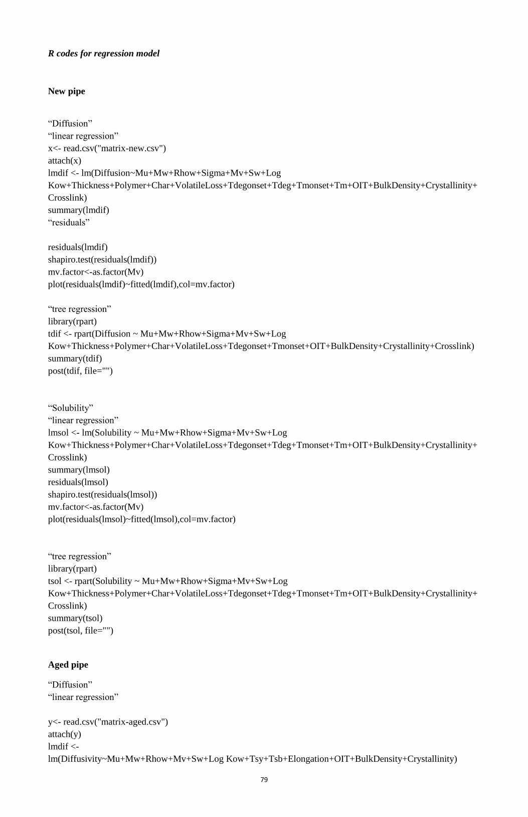
79
R codes for regression model
New pipe
―Diffusion‖
―linear regression‖
x<- read.csv("matrix-new.csv")
attach(x)
lmdif <- lm(Diffusion~Mu+Mw+Rhow+Sigma+Mv+Sw+Log
Kow+Thickness+Polymer+Char+VolatileLoss+Tdegonset+Tdeg+Tmonset+Tm+OIT+BulkDensity+Crystallinity+
Crosslink)
summary(lmdif)
―residuals‖
residuals(lmdif)
shapiro.test(residuals(lmdif))
mv.factor<-as.factor(Mv)
plot(residuals(lmdif)~fitted(lmdif),col=mv.factor)
―tree regression‖
library(rpart)
tdif <- rpart(Diffusion ~ Mu+Mw+Rhow+Sigma+Mv+Sw+Log
Kow+Thickness+Polymer+Char+VolatileLoss+Tdegonset+Tmonset+OIT+BulkDensity+Crystallinity+Crosslink)
summary(tdif)
post(tdif, file="")
―Solubility‖
―linear regression‖
lmsol <- lm(Solubility ~ Mu+Mw+Rhow+Sigma+Mv+Sw+Log
Kow+Thickness+Polymer+Char+VolatileLoss+Tdegonset+Tdeg+Tmonset+Tm+OIT+BulkDensity+Crystallinity+
Crosslink)
summary(lmsol)
residuals(lmsol)
shapiro.test(residuals(lmsol))
mv.factor<-as.factor(Mv)
plot(residuals(lmsol)~fitted(lmsol),col=mv.factor)
―tree regression‖
library(rpart)
tsol <- rpart(Solubility ~ Mu+Mw+Rhow+Sigma+Mv+Sw+Log
Kow+Thickness+Polymer+Char+VolatileLoss+Tdegonset+Tdeg+Tmonset+Tm+OIT+BulkDensity+Crystallinity+
Crosslink)
summary(tsol)
post(tsol, file="")
Aged pipe
―Diffusion‖
―linear regression‖
y<- read.csv("matrix-aged.csv")
attach(y)
lmdif <-
lm(Diffusivity~Mu+Mw+Rhow+Mv+Sw+Log Kow+Tsy+Tsb+Elongation+OIT+BulkDensity+Crystallinity)

80
summary(lmdif)
―residuals‖
residuals(lmdif)
shapiro.test(residuals(lmdif))
mv.factor<-as.factor(Mv)
plot(residuals(lmdif)~fitted(lmdif),col=mv.factor)
―tree regression‖
library(rpart)
tdif <- rpart(Diffusivity ~ Mu+Mw+Rhow+Mv+Sw+Log
Kow+Tsy+Tsb+Elongation+OIT+BulkDensity+Crystallinity)
summary(tdif)
post(tdif, file="")
―Solubility‖
―linear regression‖
lmsol <- lm(Solubility ~ Mu+Mw+Rhow+Mv+Sw+Log
Kow+Tsy+Tsb+Elongation+OIT+BulkDensity+Crystallinity)
summary(lmsol)
residuals(lmsol)
shapiro.test(residuals(lmsol))
mv.factor<-as.factor(Mv)
plot(residuals(lmsol)~fitted(lmsol),col=mv.factor)
―tree regression‖
library(rpart)
tsol <- rpart(Solubility ~ Mu+Mw+Rhow+Mv+Sw+Log
Kow+Tsy+Tsb+Elongation+OIT+BulkDensity+Crystallinity)
summary(tsol)
post(tsol, file="")

81
Experimental data for copper speciation
Appendix A-8 Copper speciation by MINEQL+
Total Cu pH 5.5 6 6.5 7 7.5
Free Cu 6.94 1.75 0.42 0.044387 0.004439
10mg/L total soluble 7.72 2.21 0.73 0.16 0.07
Cu3(PO4)2 2.28 7.79 3.01 0 0
Malachite 0 0 6.26 0 0
Tenorite 0 0 0 9.84 9.93
5mg/L Free Cu 4.49 1.62 0.41 0.044387 0.004439
total soluble 5 2.065 0.725 0.16 0.075
Cu3(PO4)2 0 2.935 1.7 0 0
Tenorite 0 0 2.575 4.84 4.925
2.5mg/L Free Cu 2.245 1.56 0.4075 0.045 0.004439
total soluble 2.5 2.005 0.725 0.16 0.0725
Cu3(PO4)2 0 0.495 1.0475 0 0
Tenorite 0 0 0.7275 2.34 2.4275
Appendix A-9 Free copper concentration in artificial saliva with different concentration of total copper and proteins; all the data are based on triplicate
samples
pH 5.5 6 6.5 7 7.5
10-inorganic 8.393205 5.057785 1.203762 0.251196 0.049564
10-inorganic-amylase 7.140667 5.190403 1.942438 0.426867 0.089077
10-amylase 8.393205 6.42486 2.930565 0.899837 0.182589
5-inorganic 4.79255 4.085994 1.203762 0.264537 0.05661
5-inorganic-amylase 2.53216 1.448939 0.745992 0.278985 0.082075
5-amylase 2.53216 1.489034 0.670749 0.264537 0.058866
2.5-inorganic 1.869968 1.585567 0.647917 0.141791 0.030288
2.5-inorganic-amylase 0.474331 0.151851 0.038085 0.008154 0.001339
2.5-amylase 0.588818 0.147678 0.034144 0.004845 0.000809
10-inorganic 8.393205 5.057785 1.203762 0.251196 0.049564
10-inorganic-mucin 0.34485 0.088888 0.016654 0.002524 0.000416
10-mucin 0.58726 0.119163 0.019662 0.002524 0.000264
5-inorganic 4.79255 4.085994 1.203762 0.264537 0.05661
5-inorganic-mucin 0.104259 0.023594 0.003761 0.000634 0.000116
5-mucin 0.177547 0.027736 0.003668 0.000439 6.44E-05
2.5-inorganic 1.869968 1.585567 0.647917 0.141791 0.030288
2.5-inorganic-mucin 0.151851 0.03333 0.006563 0.00113 0.000206
2.5-mucin 0.261005 0.02675 0.005256 0.000458 0.000106
Appendix A-10 Free copper concentration in artificial saliva with different concentration of mucin
pH 5.5 6 6.5 7 7.5
MV
inorg+0%mucin 285.5 275.5 260 244 227
inorg+10%mucin 284 281 266 248 231
inorg+50%mucin 280 275 265 251 234
inorg+70%mucin 276 268 257 245 229
inorg+100&mucin 273 260 246 229 210
Concentration ( mg/L)
inorganics+0%mucin 3.373643 1.534067 0.45222 0.128157 0.033567
inorganics+10%mucin 2.997512 2.36638 0.725608 0.175648 0.046006
inorganics+50%mucin 2.187051 1.474795 0.670621 0.222495 0.058276
inorganics+70%mucin 1.595721 0.84948 0.357004 0.138665 0.039297
inorganics+100%mucin 1.259739 0.45222 0.150035 0.039297 0.008792

82
Appendix A-11 Free copper concentration in nanopure water at different pHs
pH 5.5 6 6.5 7 7.5
10mg/l mV 325 324 319 291 279
C (mg/L) 10 9.51 6.41 0.702 0.272
5mg/l mV 316 313 298 286 272
C (mg/L) 5 3.99 1.22 0.473 0.157
2.5mg/l mV 307 305 290 281 270
C (mg/L) 2.48 2.12 0.649 0.319 0.134
Appendix A-12 Free copper concentration in saliva with different concentration of lactoferrin
pH 5.5 6 6.5 7 7.5
inorganic 297 291 272 253 232
Inorganic & Lac 298 289 268 249 233
only Lac 299 298 285 277 258
10 times Lac 296 296 293 279 265
5.5 6 6.5 7 7.5
Inorganics 8.350108 5.204023 1.164274 0.260478 0.049778
inorganics & Lac 9.03478 4.445169 0.84948 0.190051 0.053859
Only Lac 9.775592 9.03478 3.243294 1.726564 0.386277
10 times Lac 7.717322 7.717322 6.092425 2.021313 0.670621
Appendix A-13 pH and free copper changes with time
time/min pH mV C(mg/L)
0.5 6.63 260 0.521172
1 6.65 259 0.48045
5 6.7 256 0.376399
10 6.74 255 0.346989
20 6.81 251 0.250601
30 6.88 249 0.212969
60 6.93 245 0.15381
120 7.19 234 0.062852
180 7.22 230 0.045393


![Air Contaminant _54.12_ [Preamb]](https://static.fdocuments.net/doc/165x107/5695cf481a28ab9b028d6988/air-contaminant-5412-preamb.jpg)


