Modeling and Linear Parameter-Varying Identification of a ...
84
UNIVERSIDADE FEDERAL DO CEARÁ CENTRO DE TENCOLOGIA DEPARTAMENTO DE ENGENHARIA ELÉTRICA PROGRAMA DE PÓS-GRADUAÇÃO EM ENGENHARIA ELÉTRICA FÉLIX EDUARDO MAPURUNGA DE MELO MODELING AND LINEAR PARAMETER-VARYING IDENTIFICATION OF A TWO-TANK SYSTEM FORTALEZA 2017
Transcript of Modeling and Linear Parameter-Varying Identification of a ...

UNIVERSIDADE FEDERAL DO CEARÁCENTRO DE TENCOLOGIA
DEPARTAMENTO DE ENGENHARIA ELÉTRICAPROGRAMA DE PÓS-GRADUAÇÃO EM ENGENHARIA ELÉTRICA
FÉLIX EDUARDO MAPURUNGA DE MELO
MODELING AND LINEAR PARAMETER-VARYING IDENTIFICATION OF ATWO-TANK SYSTEM
FORTALEZA
2017

FÉLIX EDUARDO MAPURUNGA DE MELO
MODELING AND LINEAR PARAMETER-VARYING IDENTIFICATION OF ATWO-TANK SYSTEM
Master’s dissertation presented to the graduateprogram in Electrical Engineering from FederalUniversity of Ceará as part of the requisites toobtain the Master’s degree in Electrical Engi-neering. Concentration Area: Electrical Energysystems.
Supervisor: Prof. Fabrício Gonzalez NogueiraCo-supervisor: Prof. Arthur P. de Souza Braga
FORTALEZA
2017

Dados Internacionais de Catalogação na Publicação Universidade Federal do Ceará
Biblioteca UniversitáriaGerada automaticamente pelo módulo Catalog, mediante os dados fornecidos pelo(a) autor(a)
M485m Melo, Félix Eduardo Mapurunga de. Modeling and linear parameter-varying identification of a two-tank system / Félix Eduardo Mapurungade Melo. – 2017. 82 f. : il. color.
Dissertação (mestrado) – Universidade Federal do Ceará, Centro de Tecnologia, Programa de Pós-Graduação em Engenharia Elétrica, Fortaleza, 2017. Orientação: Prof. Dr. Fabrício Gonzalez Nogueira. Coorientação: Prof. Dr. Arthur Plínio de Souza Braga.
1. Linear com Parâmetros Variantes. 2. Identificação de Sistemas. 3. Sistemas de dois tanques. 4.Modelagem. 5. Máquinas de vetor de suporte. I. Título. CDD 621.3

FÉLIX EDUARDO MAPURUNGA DE MELO
MODELING AND LINEAR PARAMETER-VARYING IDENTIFICATION OF ATWO-TANK SYSTEM
Master’s dissertation presented to the graduateprogram in Electrical Engineering from FederalUniversity of Ceará as part of the requisites toobtain the Master’s degree in Electrical Engi-neering. Concentration Area: Electrical Energysystems.
Approved in July 18, 2017.
EXAMINATION BOARD
Prof. Fabrício Gonzalez Nogueira (Supervisor)Universidade Federal do Ceará
Prof. Arthur P. de Souza Braga (Co-supervisor)Universidade Federal do Ceará
Prof. Wilkley Bezerra CorreiaUniversidade Federal do Ceará
Prof. Guilherme de Alencar BarretoUniversidade Federal do Ceará
Prof. José Everardo Bessa MaiaUniversidade Estadual do Ceará

ACKNOWLEDGEMENTS
I would like to express my gratitude to my supervisor, who introduced me to the themeand have supported me to continue my research path in the system identification field. It was agreat pleasure to work with Fabrício during these two years. He provided me not only with hisexpertise, but also with valuable hints in many aspects of life itself, whose I will carry with mefor my entire life as well as his friendship.
I am eternally grateful to my family, who I own everything. Firstly, my not so patientwife, whose love and care always revitalized me every day and filled me with energy to conqueranything in my life. Secondly, my mother that started this journey and have always expressed allthe support necessary in my life. Last but not the least, my beloved sister that both of us knowwe can always count on each other.
Throughout this work I have met many people that have helped me in some way. Then,I would like to thank the professors associated with the GPAR laboratory, which I have spentmore time with. The first contribute came from my co-supervisor prof. Arthur, which I have hadthe chance to learn (and have fun) about computational intelligence. Prof. Bismarck deservesa special thanks for the clarifying talks about systems and predictive control, as well as thedevelopment of this work. Profa Laurinda that always made the possible to help me in manyissues during this period. Unfortunately, she could not participate in this final stage. Finally, Prof.Wilkley whom I have had fewer time with, but his contributes to this work made the difference.For aforementioned reasons it goes my sincerely thanks.
I would like to thank the examination board, composed by Prof. José Everardo BessaMaia and Prof. Guilherme de Alencar Barreto, for the time spent in analyzing this work. Aspecial thanks goes to Prof. Everardo, who introduced me to the system identification field andthe unmeasurable guidance inspired me to take this path in my life.
If I list all the reasons to be grateful to my friends for everything they have done thissection would have more pages than the entire work. I simply do not dare to translate in wordsthe shared moments we have had together. Then, I have chosen to name each one of you inalphabetical order: Adriano, Aluisio, Caio, Clauson, Fábio, Paulo, Magno, René, and Silas.Each one of you know exactly what you have made for me. A special thanks goes to my friendMatheus for kindly revising this text.
Last but not the least, this work would not be possible without the financial add fromCAPES. Therefore, I am grateful to CAPES for the substantial support throughout this phase ofmy life.

ABSTRACT
This work addresses the modeling and the linear parameter-varying (LPV) system identificationof a coupled two-tank system (TTS). The system is a multiple input multiple output (MIMO) withtwo inputs and two outputs. In order to obtain a suitable model for this system, a first-principleapproach based on the mass balance principle is followed. It turns out that the modeling processwas driven by the geometrical shape of the tanks. Thus, most of its parameters are based onthe tanks’ dimensions. When it comes to the LPV identification, several methods are presentedranging from the classical results from the regression approach to the current support vectormachines (SVM) based methods. All the identification algorithms presented are extended inorder to cope with the MIMO systems. Additionally, a method based on instrumental variablessupport vector machines was adapted from the general nonlinear case to the LPV case. A newLPV model with two independent scheduling variables is proposed driven by prior knowledgeon the process model. The results obtained with this new LPV model have showed a goodperformance in describing the TTS behavior. Furthermore, they were better than an LPV modelconsidering only a single scheduling variable.
Keywords: two-tank system. LPV system identification.

RESUMO
Este trabalho lida com a modelagem e identificação com abordagem de sistemas com parâmetrosvariantes (LPV) de um sistema de dois tanques acoplados (TTS). Esse sistema é do tipo múltiplaentrada múltipla saída (MIMO) com duas entradas e duas saídas. Com a finalidade de obterum modelo adequado para esse sistema, é feita uma abordagem fenomenológica baseada noprincípio do balanço de massa. Descobre-se que o processo de modelagem é dependente daforma geométrica dos tanques. Assim, a maioria dos seus parâmetros são baseados nas dimensõesdos tanques. Quando se trata de identificação de sistemas LPV, vários métodos são apresentadosdesde os resultados clássicos baseados em regressão até os métodos atuais baseados em máquinasde vetor de suporte. Todos os algoritmos de identificação apresentados são estendidos para lidarcom sistemas MIMO. Além disso, um método baseado em variáveis instrumentais com máquinasde vetor de suporte foi adaptado do caso não linear geral para o caso LPV. Um novo modeloLPV com duas variáveis de scheduling é proposto baseado em conhecimento a priori no modelodo processo. Os resultados obtidos com esse novo modelo LPV mostraram bom desempenho aodescrever o comportamento do sistema de dois tanques. Ademais, eles foram melhores do queum modelo LPV considerando apenas uma variável de scheduling.
Palavras-chave: Sistemas de dois tanques. Identificação de modelos LPV.

LIST OF FIGURES
Figure 1 – The Identification procedure . . . . . . . . . . . . . . . . . . . . . . . . . . 14Figure 2 – The Two-Tank System . . . . . . . . . . . . . . . . . . . . . . . . . . . . . 22Figure 3 – Isolated Tank 1 System . . . . . . . . . . . . . . . . . . . . . . . . . . . . 23Figure 4 – Isolated Tank 2 System . . . . . . . . . . . . . . . . . . . . . . . . . . . . 25Figure 5 – A truncated cone . . . . . . . . . . . . . . . . . . . . . . . . . . . . . . . . 26Figure 6 – SHURFLO Pump . . . . . . . . . . . . . . . . . . . . . . . . . . . . . . . 28Figure 7 – Schematic of the pump driver . . . . . . . . . . . . . . . . . . . . . . . . . 28Figure 8 – Operation range of the pumps . . . . . . . . . . . . . . . . . . . . . . . . . 29Figure 9 – Flow Sensor Model YF-S201 . . . . . . . . . . . . . . . . . . . . . . . . . 29Figure 10 – Output of the flow sensors . . . . . . . . . . . . . . . . . . . . . . . . . . . 30Figure 11 – Differential pressure sensor . . . . . . . . . . . . . . . . . . . . . . . . . . 30Figure 12 – Curve voltage versus differential pressures . . . . . . . . . . . . . . . . . . 31Figure 13 – Valve’s aperture measurement . . . . . . . . . . . . . . . . . . . . . . . . . 31Figure 14 – LPV System . . . . . . . . . . . . . . . . . . . . . . . . . . . . . . . . . . 34Figure 15 – Signal flow of the general LPV system descriptor . . . . . . . . . . . . . . 37Figure 16 – MISO interpretation of an LPV system . . . . . . . . . . . . . . . . . . . . 46Figure 17 – The margin in the SVM framework . . . . . . . . . . . . . . . . . . . . . . 49Figure 18 – k12 in the range of p . . . . . . . . . . . . . . . . . . . . . . . . . . . . . . 58Figure 19 – PRBS design using the logic xor . . . . . . . . . . . . . . . . . . . . . . . 60Figure 20 – The step response of the system . . . . . . . . . . . . . . . . . . . . . . . . 61Figure 21 – Periodogram of the designed PRBS . . . . . . . . . . . . . . . . . . . . . . 62Figure 22 – DE - Input and Scheduling variable . . . . . . . . . . . . . . . . . . . . . . 63Figure 23 – DE - Outputs . . . . . . . . . . . . . . . . . . . . . . . . . . . . . . . . . . 63Figure 24 – Results for the LPV-TTS with the RIV method on DIV . . . . . . . . . . . . 70Figure 25 – Results for the LPV3S-TTS with the IV method on DIV . . . . . . . . . . . 71Figure 26 – Input and scheduling sequence of DIV . . . . . . . . . . . . . . . . . . . . 71
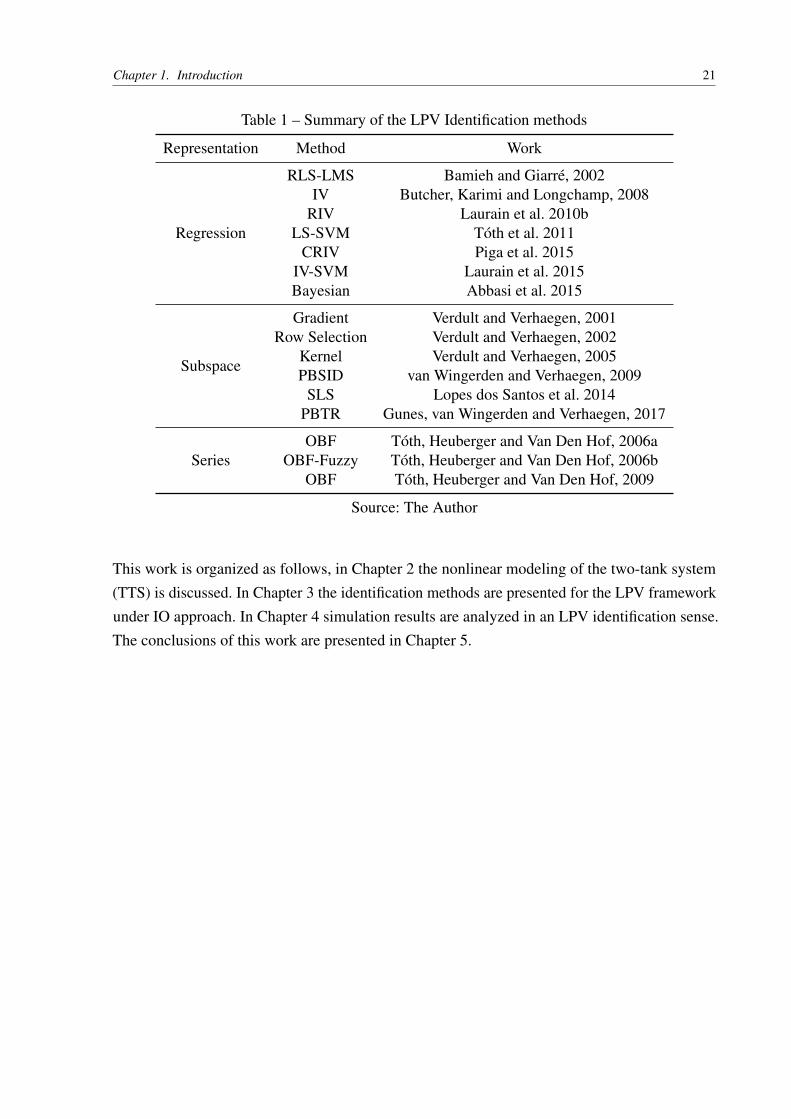
LIST OF TABLES
Table 1 – Summary of the LPV Identification methods . . . . . . . . . . . . . . . . . 21Table 2 – Data set from Tank 1’s valve . . . . . . . . . . . . . . . . . . . . . . . . . . 32Table 3 – Data set from Tank 2’s valve . . . . . . . . . . . . . . . . . . . . . . . . . . 32Table 4 – Choice of the nonzero elements in A(q) for the PRBS design . . . . . . . . . 60Table 5 – Results on the Validation data set . . . . . . . . . . . . . . . . . . . . . . . 65Table 6 – Results of the models for a single tank . . . . . . . . . . . . . . . . . . . . . 67Table 7 – Results on the Validation data set with SNR = 30dB . . . . . . . . . . . . . 69Table 8 – Parameters of the models obtained . . . . . . . . . . . . . . . . . . . . . . . 70Table 9 – BFS for the obtained models . . . . . . . . . . . . . . . . . . . . . . . . . . 72

LIST OF ABBREVIATIONS AND ACRONYMS
ARMA Autoregressive-Moving Average
ARX Autoregressive with Exogenous Output
BFS Best Fit Score
BJ Box Jenkins
IO Input-Output
IR Impulse Response
IV Instrumental Variable
IV-SVM Instrumental Variable Support Vector Machines
IVM Instrumental Variable Method
LS Least Squares
LS-SVM Least Squares Support Vector Machines
LMS Least Mean Squares
LPV Linear Parameter-Varying
LTI Linear Time Invariant
MIMO Multiple Input Multiple Output
OBF Orthonormal Basis Functions
OE Output Error
PE Prediction Error
PEM Prediction Error Method
PES Persistently Exciting Signal
PID Proportional Integral Derivative
q-LPV Quasi-Linear Parameter-Varying
QP Quadratic Programming
RBF Radial Basis Function

RIV Refined Instrumental Variable
RLS Recursive Least Squares
SISO Single Input Single Output
SS State-Space
SVM Support Vector Machines
TTS Two-Tank System

LIST OF SYMBOLS
P Scheduling space
R Real set
Z Integers set
D Data set
E Mathematical expectation
L Lagrangian
M Model
e White noise
G Process Filter
h water height
H Noise Filter
k Valve constant (Tank models), discrete time
p Scheduling variable
q Volumetric flow-rate, Time shift operator
r Radius
u Input of a model
v Noise process
v Nonlinear mapping
V Volume, Quadratic error cost function
y Output of a model
α Learning rate (LMS), Lagrangian multipliers (LS-SVM)
γ Regularization parameter
ζ Instrumental variable vector
η Parameter vector related to the noise filter

θ Parameters vector
ρ Specific mass, Parameter vector related to the process filter
ϕ Regressors vector
Φu(ω) Spectrum of the signal u
ψ Basis function
ω Mass flow-rate, Parameter vector (LS-SVM)
Ω Kernel matrix (LS-SVM)

CONTENTS
1 INTRODUCTION . . . . . . . . . . . . . . . . . . . . . . . . . . . . . . 131.1 The System Identification Problem . . . . . . . . . . . . . . . . . . . . . 141.2 State-of-the-Art in LPV System Identification . . . . . . . . . . . . . . . 161.3 The Present Work . . . . . . . . . . . . . . . . . . . . . . . . . . . . . . 202 TWO-TANK SYSTEM MODELING . . . . . . . . . . . . . . . . . . . . 222.1 Overview of the System . . . . . . . . . . . . . . . . . . . . . . . . . . . 222.2 Mathematical Model of the Tank 1 . . . . . . . . . . . . . . . . . . . . . 232.3 Mathematical Model of the Tank 2 . . . . . . . . . . . . . . . . . . . . . 252.4 Mathematical Model of the TTS . . . . . . . . . . . . . . . . . . . . . . . 272.5 The Measurement and Actuator Systems . . . . . . . . . . . . . . . . . . 272.6 The Experimental setup . . . . . . . . . . . . . . . . . . . . . . . . . . . 312.7 Summary of the Chapter . . . . . . . . . . . . . . . . . . . . . . . . . . . 323 THE LINEAR PARAMETER-VARYING SYSTEM IDENTIFICATION 333.1 LPV Systems . . . . . . . . . . . . . . . . . . . . . . . . . . . . . . . . . 333.2 LPV Model Structures . . . . . . . . . . . . . . . . . . . . . . . . . . . . 343.3 LPV Identification Approaches . . . . . . . . . . . . . . . . . . . . . . . 353.4 The Regression Approach . . . . . . . . . . . . . . . . . . . . . . . . . . 363.5 The Correlation Approach . . . . . . . . . . . . . . . . . . . . . . . . . . 433.6 The LS-SVM approach . . . . . . . . . . . . . . . . . . . . . . . . . . . . 483.7 The IV Method in the LS-SVM Framework . . . . . . . . . . . . . . . . 543.8 Summary of the Chapter . . . . . . . . . . . . . . . . . . . . . . . . . . . 564 SIMULATION RESULTS . . . . . . . . . . . . . . . . . . . . . . . . . . 574.1 Simulation Setting . . . . . . . . . . . . . . . . . . . . . . . . . . . . . . 574.2 Input Design . . . . . . . . . . . . . . . . . . . . . . . . . . . . . . . . . 584.3 Identification Experiment in the Simulation Setting . . . . . . . . . . . . 604.4 Model Structure . . . . . . . . . . . . . . . . . . . . . . . . . . . . . . . 634.5 Results . . . . . . . . . . . . . . . . . . . . . . . . . . . . . . . . . . . . . 644.6 A Single Tank in the LPV Framework . . . . . . . . . . . . . . . . . . . 664.7 An LPV Model with 2 Scheduling Variables . . . . . . . . . . . . . . . . 674.8 The TTS with 3 Scheduling Variables . . . . . . . . . . . . . . . . . . . . 684.9 The Final Choice . . . . . . . . . . . . . . . . . . . . . . . . . . . . . . . 684.10 Summary of the Chapter . . . . . . . . . . . . . . . . . . . . . . . . . . . 715 CONCLUSION . . . . . . . . . . . . . . . . . . . . . . . . . . . . . . . . 73
BIBLIOGRAPHY . . . . . . . . . . . . . . . . . . . . . . . . . . . . . . 76

13
1 INTRODUCTION
During many years the linear time invariant(LTI) framework has dominated the industry,mainly due to its simplicity and good performance. In fact, the LTI approach has been of suchparamount importance to this date that, according to Åström and Hägglund (1995) in the ninetiesabout 90% of the control loops were of PID type, and the use of this approach has never droppedsince then. However, the increasing quest for performance requires a framework that is stillsimple but has better representative behavior of the nonlinear dynamics.
The Linear Parameter-Varying (LPV) systems are inspired in the gain-scheduling strategy(ÅSTRÖM; WITTENMARK, 1994), which consists in the point of view that a nonlinear systemcan be represented as a collection of LTI systems where each system represents an operationcondition. The LPV framework is intended to play the role of the bridge between the lack ofgeneral structure in nonlinear systems and the well organized world of linear systems. The LPVsystems preserve the linear behavior between input and output for a constant scheduling variable,which is usually an exogenous signal related to the system’s working point.
The LPV class cope with nonlinearities with the advantage of a linear formulation. Thismakes the LPV models an attractive candidate to model nonlinear behavior and time-varyingphenomena. The challenges of today’s industry are driving the search for more accurate models.Besides, nowadays the industry requires an ability to cope with systems in many industrialscenarios, such as plants working in a wide range of operation points. This usually requires thatthe controller have adaptive properties. The LPV framework offers a representative system classto deal with these new challenges. In fact, the LPV model class can be viewed as an extension ofthe linear time varying (LTV) class (TÓTH, 2010).
In order to make clear the paramount importance of the scheduling variable in the LPVframework, consider a model of an aircraft. This system has three inputs, the elevator, canard,and leading edge flaps, in which the pilot can control the pitch movement of the aircraft. Theseinputs are related to devices in the wings that control the direction of air flow through the wings.Thus, a model that relates these inputs with the pitch rate can be built (or identified) to describethe dynamic behavior of the system. However, the flight dynamics changes according to thealtitude of the aircraft. In this way, the model is naturally influenced by the altitude. In thisexample, the altitude is an exogenous signal that is directly related to the operational condition ofthe system. Moreover, the pilot can not avoid the influence of the altitude in the system dynamics.The pitch control system of the aircraft can be considered as an LPV model with the altitudeplaying the role of scheduling variable.
This chapter is organized as follows. In the first section the system identification problemis presented and its steps are given. The second section describes the state-of-the-art of LPV

Chapter 1. Introduction 14
system identification. The third section presents the current work and its objectives.
1.1 The System Identification Problem
The system identification problem can be stated as follows. Given a data set of input-output measurements DN = u(k),y(k)N
k=1, a model structure and a fitness criterion, typicallya cost function based on the model error, find the best model among all feasible models in thecollection that best describes the input-output behavior of the system at hand (LJUNG, 1999).These three entities together form the basic core of the system identification itself.
Although identification of dynamical systems has a well-defined logical flow, there areseveral considerations that one must take in order to successfully identify a representative model.There is a natural logical procedure to the system identification task. Figure 1 illustrates theidentification scheme, which has a cycled nature. In the following, a brief overview of each step
Figure 1 – The Identification procedure
Find the best model
Data Collection
Choice of the Model Structure
Choice of the Criterion
Experiment Design
Validate the model
Passed?
Use it!
No
Yes
Source: The Author
is given.
Experiment Design and Data Collection
In this step the user must answer some questions, such as: which are input and outputsignals, how to collect these data, when will it be collected, is there any signal conditioning tobe made. Additionally, there is the question of selecting an appropriate input in order to givevaluable information about the system to be modeled. One input that produces an output withenough information content is said to be a persistently exciting signal (PES). The latter questionis known as experiment design. In addition to the information problem, the signal to be used asinput generally needs to be feasible due to practical issues, e.g. input constraints. Another focusof the experiment design related to PES is how to produce informative data sets, which musthave enough information content to distinguish between different models in the model collection

Chapter 1. Introduction 15
(informativity is a property of a data set and it is dependent on the model structure. PES is aproperty of a signal and it is independent of the model structure). In some cases the user doesn’thave the possibility to interfere in the system variables at hand and there are other cases wherethe user must design a controller in order to make the experiment, e.g. unstable plants. Datapreprocessing is another issue to be dealt with, which focuses on attenuation of disturbances,removal of trends, exclusion of outliers, and noise effects in data.
Choice of the Model Structure
In this part of the identification procedure a model structure must be chosen and it willdetermine the set of models that one is searching for the best model. In this step, questionsconcerning the representation form of the model (State-Space (SS), input-output (IO), series-expansion, etc.), parametrization, type of noise modeling, and choice of the model order, must beanswered. Here, a priori knowledge and engineering insight must be combined to carefully adjustthe model towards its actual behavior. The model structure is directly related to the algorithmthat selects the best model in the set. Therefore, questions like existence of local optimal mustbe considered within the choice of the set of candidates. The complexity of the model (e.g. thenumber of parameters in the model) is related to the well-known bias-variance trade off. Hence,this question must be considered as well in the choice of the model structure.
Choice of the Identification Criterion
It consists in selecting a performance criteria in order to classify the models in the modelset. The assessment of model quality is generally based on the performance of the model whenattempting to reproduce the data. The user must look for a criterion that is able to select in themodel set the model which best describes the measured data set DN . Usually, in the systemidentification literature, a quadratic norm of the error of the output prediction of the modelestimate is chosen (LJUNG, 1999).
Selection of the Best Model
In this phase an algorithmic solution (a mathematical expression that delivers the bestmodel) is obtained in terms of model structure and the identification criterion selected. It is inthis step, also known as identification method, that the best model is chosen. The method itselfcan be obtained from an algebraic or a probabilistic point of view among other mathematicalperspectives. It must be noticed that the method selects the best model in the model set accordingto one’s chosen identification criterion and that is an important part of the identification cycle,but it is not the most essential one.
Chapter 1. Introduction 16
Model (in)validation
This step is where one must confront the model with some procedures in order to decidewhether the model can be accepted. This question is directly related with the user’s purposes forthe model. The model should pass some tests that involve how the model relates to observeddata, prior knowledge of the system at hand, and its intended use. Such tests are known as modelvalidation. The model that presents poor behavior confronted with the data should be discardedand the identification cycle must run once again from the first step in order to obtain anothermodel.
The System Identification Paths
The system identification procedure has a very clear logical flow. Firstly, collect the dataand choose a model set. Secondly, pick the best model in the model set according to a chosencriterion. Finally, perform the tests in order to validate the model. If the model passes, thenaccept the model, else repeat the procedure using different choices from the beginning. Themodel may be deficient for many reasons including (LJUNG, 1999):
a) The identification method failed to find the best model according to the identificationcriterion;
b) The identification criterion was not well-chosen;
c) The model structure was not appropriate, that is, it didn’t provide any good descriptionin the model set;
d) The data set was not informative enough.
It is important to understand how the system identification has developed before entering inthe LPV identification framework. Basically, when the system descriptor is expressed in the IOsetting, the identification problem is formulated through a regression approach. When it comesto SS representation, the system identification is mainly focused on subspace methods, that is,the identification problem is based on certain space projections, see (VAN OVERSCHEE; DEMOOR, 1996) for a detailed overview. The LPV system identification naturally followed thedevelopments of the LTI framework, with the necessary adaptations, of course. The reason liesbasically in the fact that LPV models can be seen as an extension of the LTI models, then themost natural way to develop the LPV system identification was to extend the LTI results.
1.2 State-of-the-Art in LPV System Identification
A brief resume of the LPV identification developments is necessary in order to understandwhat it has done and what may still be coming. Similarly, the LPV identification followed thetwo basic procedures of the LTI framework, which are dependent on the system representation.In the case of the IO setting, the LPV framework was done exclusively in the regression form,

Chapter 1. Introduction 17
whereas for the SS representation the natural extension was the subspace approach. Due to thelack of transfer function representation in the LPV framework, the LPV identification emergedbased on an algorithmic sense, that is, the first works in the LPV identification literature arebased on optimization problems, such as (BAMIEH; GIARRÉ, 1999b; BAMIEH; GIARRÉ,1999a; LEE; POOLLA, 1996; LEE; POOLLA, 1999). In fact, the very first attempt to addressthe LPV identification problem was done in (NEMANI; RAVIKANTH; BAMIEH, 1995). In thatwork it was assumed full knowledge of the state sequence and considered only one schedulingvariable. In (PREVIDI; LOVERA, 1999) it is attempted to solve the problem by separatingthe linear and nonlinear parts. The former was performed in a regression form, the latter byusing an artificial neural network. Another approach was a robust identification via worst-caseidentification presented in (MAZZARO; MOVSICHOFF; SÁNCHEZ-PEÑA, 1999).
The Least Mean Squares(LMS) and the Recursive Least Squares(RLS) were introduced in(BAMIEH; GIARRÉ, 1999b; BAMIEH; GIARRÉ, 1999a) for the LPV identification framework.However, differently of the LTI counterpart, for the regression approach in the LPV identificationit is necessary to define a parametrization of the scheduling variable. That is, the model outputmust be linear in parameters(necessary condition for linear regression problems), and eachregressor must be defined as a function of the scheduling variable. Here are defined the basisfunctions that play an important role in the LPV system identification framework. These basisfunctions are part of the user’s choice and give a huge degree of freedom compared to theLTI case, common choices are polynomial and periodic functions such as sine. In (BAMIEH;GIARRÉ, 2002) the identification was investigated using a polynomial basis and an introductoryresult of persistently excitation signals was presented for the polynomial dependence case.
The first subspace approach for the LPV identification was addressed in (VERDULT;VERHAEGEN, 2001), but still with its roots in the optimization problem. A huge drawbackof the subspace approach in the LPV framework is the curse of dimensionality, usually thedimensions of the data matrices involved grow exponentially. In fact, the subspace approachin the LPV case was inspired by the subspace identification procedures developed for bilinearsystems. Usually, in the subspace approach for LPV systems, it is commonly assumed thatthe matrices involved have an affine dependence on the scheduling variable. In (VERDULT;VERHAEGEN, 2002) it was presented an extension of the subspace approach used in the bilinearsystems to the LPV case. In that work a first step was taken in order to overcome the curse ofdimensionality, a procedure was given to select a subset of the most dominant rows from thedata matrices. Another successful approach to avoid the curse of dimensionality in the subspaceapproach was the use of the Kernel trick to avoid unnecessary matrix computations as introducedin (VERDULT; VERHAEGEN, 2005).
Another approach to represent LTI systems is through orthonormal basis functions (OBF)representation. This kind of representation appeared in the LTI framework, see (HEUBERGER;VAN DEN HOF; WAHLBERG, 2005) for an overview, and it was initially introduced in the

Chapter 1. Introduction 18
LPV case in (TÓTH; HEUBERGER; VAN DEN HOF, 2006a). In sequence a fuzzy clusteringapproach was developed to select pole locations for OBFs in the LPV identification problemin (TÓTH; HEUBERGER; VAN DEN HOF, 2006b). As the LPV models can be seen as acollection of LTI models, many of the identification problems are solved as identification of localLTI models and then interpolation is applied in order to obtain the LPV model. In this way, LPVmodels can be viewed under two perspectives: the global and the local approach. The formerconsists in identifying an LPV model trying to capture the dynamic relationship of the systemwith a varying scheduling parameter. The latter considers the identification of many local LTImodels (at a constant scheduling variable) and then it applies an interpolation scheme to obtainthe global model.
The subspace approach continued giving results based on a convergent sequence oflinear deterministic-stochastic state space approximations in (LOPES DOS SANTOS; RAMOS;MARTINS DE CARVALHO, 2007). Many of the subspace methods presented take advantage ofthe LTI subspace approach, as in (FELICI; VAN WINGERDEN; VERHAEGEN, 2007) where asubspace method was developed capable of determining the deterministic part of an LPV-SSsystem in the presence of output error, one of the key aspects was to ensure that the schedulingvariable must be periodic, it turned out this made the algorithm more computationally efficient. Aglobal and local approach to identify LPV systems based on OBFs representation was introducedin (TÓTH; HEUBERGER; VAN DEN HOF, 2007).
Neither of the identification approaches presented so far dealt with LPV systems in theview of system theory. Moreover, all of these approaches didn’t hold any connections. Thismeans that there were no concerns about the differences between IO and SS domains. It wasonly with the development of LPV system theory initially introduced in (TÓTH et al., 2007)that the IO domain and the SS representation were connected via a realization theory through anaffine canonical representation for LPV-SS models similar to the LTV framework. As a matterof fact, many of the control and interpolation based identification papers assumed that the LTIframework intuitively would extend to the LPV case. It turns out, it was demonstrated that thisextension didn’t follow as straightforward as it seemed. Until 2010, much effort had been made toestimate LPV models at light of estimation problems from LTI system identification, but only fewefforts were done to develop a proper LPV system theory. The development of the LPV systemtheory had crescent interest with the introduced study of optimal design for local experiments in(KHALATE et al., 2009), the investigation of discretization methods for the LPV framework in(TÓTH et al., 2008), state space realization methods in (ABBAS; TÓTH; WERNER, 2010), andfinally the introduced behavioral approach, see (WILLEMS, 1991) for a detailed overview, in(TÓTH et al., 2009; TÓTH et al., 2011). These works allowed a strong basis in the LPV systemtheory and, more importantly, answered questions on how LPV systems should be dealt with inthe eye of system theory. An OBF based system identification that gives enough flexibility toLPV models was presented in (TÓTH; HEUBERGER; VAN DEN HOF, 2008). In (BUTCHER;KARIMI; LONGCHAMP, 2008) the instrumental variable method was introduced in the LPV

Chapter 1. Introduction 19
framework from the LTI counterpart. Following such approach, an algorithm also from theLTI case, called refined instrumental variable method was introduced in the LPV framework(LAURAIN et al., 2010a; LAURAIN et al., 2010b). While in the subspace approach an algorithmwas developed to cope with LPV and bilinear identification in both open and closed-loop settingin (VAN WINGERDEN; VERHAEGEN, 2009). An instrumental variable method for closed-loop LPV identification was presented in (TÓTH et al., 2011; TÓTH et al., 2012) within the IOsetting. The formal introduction of the prediction error method in the LPV case was only madein (TÓTH; HEUBERGER; VAN DEN HOF, 2010). So far, most algorithms presented dealt withdiscrete time LPV models. In (LAURAIN et al., 2011a; LAURAIN et al., 2011b) the continuoustime identification of LPV systems was addressed in the IO settings.
Another strong add in the LPV system identification was the introduction of the leastsquares support vector machines (LS-SVM) from the machine learning field in (TÓTH et al.,2011). The introduction of LS-SVMs in the LPV framework was very important, mainly due tothe learning appeal and the use of Kernels that can learn the underlying parameter’s dependencywith the scheduling variable. This was a huge advantage over the general methods in regressionform, in which one must select an appropriate basis function to define the underlying relationshipbetween regressors and the scheduling variable. As the kernel method became an interestingfeature in LPV system identification in IO setting, the subspace approach made important stepstoward regularization techniques, such as in (GEBRAAD et al., 2011), where a novel approachusing nuclear norm regularization is proposed in the LPV subspace approach. The purposeremained quite the same which is to cope with the curse of dimensionality in data matrices. Infact, the use of kernels dominated the first half of the decade and it is still an active area ofresearch in the LPV identification literature. The LPV LS-SVM identification is investigatedunder general noise conditions in (LAURAIN et al., 2012). A common assumption in mostof the works presented so far is that the scheduling variable is a free noise measured signal.In (LOPES DOS SANTOS et al., 2012) an extension of the algorithm presented in (LOPESDOS SANTOS; RAMOS; MARTINS DE CARVALHO, 2009) is generalized to cope withquasi-stationary scheduling sequences. A separable least squares approach was extended to theLPV case in (LOPES DOS SANTOS et al., 2013). An algorithm that identifies the LPV orderin the LS-SVM framework was introduced in (PIGA; TÓTH, 2013). Before that, a study onLPV-ARX order selection had been done in (TÓTH; HJALMARSSON; ROJAS, 2012). Thegeneral LS-SVM for the LPV case was extended to cope with noisy scheduling variables in(ABBASI et al., 2014). The separable least squares approach was extended to the LPV LS-SVMframework in (LOPES DOS SANTOS et al., 2014).
With all the development in the kernel and regularized parameter estimation, the currentLPV system identification is now focusing toward a Bayesian perspective, initially introduced in(GOLABI et al., 2014). An identification procedure based on correlation analysis was given in(COX; TÓTH; PETRECZKY, 2015). A Gaussian process based Bayesian method that accountsfor noisy scheduling variables for LPV models in IO setting is presented in (ABBASI et al., 2015).

Chapter 1. Introduction 20
An algorithm is proposed to correctly estimate LPV models under general noise conditionsof Box-Jenkins type in the Bayesian approach in (DARWISH et al., 2015). An instrumentalvariable scheme is introduced in (PIGA et al., 2015) to cope with noise both in schedulingvariable and in system output. A new method that combines the global and local approaches inthe identification of LPV systems was given in (TURK; PIPELEERS; SWEVERS, 2015). Aninstrumental variable based on LS-SVM was introduced in (RIZVI et al., 2015b) for LPV-SSmodels. Still in the LS-SVM framework, an approach based on kernel was introduced in the SSstructure to identify multiple-input multiple-output LPV systems (RIZVI et al., 2015a). A kernelbased approach was also introduced in the subspace methodology in (PROIMADIS; BIJL; VANWINGERDEN, 2015). The Bayesian framework was also extended to the LPV-SS structure in(COX; TÓTH, 2016). A presentation in Kalman style realization theory for LPV-SS with affinedependence on the scheduling variable is given in (PETRECZKY; TÓTH; MERCERE, 2016). Amethodology to construct the kernels in the LS-SVM approach for LPV system was presentedin (ROMANO et al., 2016). Still in the LS-SVM context, a general approach for identificationof partial differential equation-governed by spatially-interconnected LPV systems was given in(LIU et al., 2016). A study of the Bayesian approach in LPV system identification to accuratelymodel nonlinear processes was given in (GOLABI et al., 2017), while in the LPV susbpaceapproach a predictor-based tensor regressor was introduced in (GUNES; VAN WINGERDEN;VERHAEGEN, 2017).
It is clear that either in the IO setting or in the SS domain the kernel-based and regular-ization approaches remain the current focus of research in academia. This intense research andthe contact with the machine learning community allowed the development of kernel methodsand the LS-SVM approach in a wide range of system identification areas. The development ofGaussian processes and the development of new kernel methods that incorporate prior informa-tion about the unknown system (PROIMADIS; BIJL; VAN WINGERDEN, 2015) attracted oncemore the research interest in the Bayesian approach for all system identification branches. Table1 presents a summary of the works presented in this section.
1.3 The Present Work
This work addresses the identification of LPV systems under the IO approach. From theclassical results of the least squares and instrumental variable method to the current state-of-the-art kernels methods. Additionally, in this work a model from first-principles(laws of physics) ofa two tank process system and its identification is set under the LPV framework. The latter taskis addressed through the simulation of the model obtained from first-principles. This work hasthe following objectives:
a) To model a nonlinear representation of a multiple input multiple output (MIMO) tanksystem;
b) Identify an LPV MIMO system for the two tank system.
Chapter 1. Introduction 21
Table 1 – Summary of the LPV Identification methods
Representation Method Work
Regression
RLS-LMS Bamieh and Giarré, 2002IV Butcher, Karimi and Longchamp, 2008
RIV Laurain et al. 2010bLS-SVM Tóth et al. 2011
CRIV Piga et al. 2015IV-SVM Laurain et al. 2015Bayesian Abbasi et al. 2015
Subspace
Gradient Verdult and Verhaegen, 2001Row Selection Verdult and Verhaegen, 2002
Kernel Verdult and Verhaegen, 2005PBSID van Wingerden and Verhaegen, 2009
SLS Lopes dos Santos et al. 2014PBTR Gunes, van Wingerden and Verhaegen, 2017
SeriesOBF Tóth, Heuberger and Van Den Hof, 2006a
OBF-Fuzzy Tóth, Heuberger and Van Den Hof, 2006bOBF Tóth, Heuberger and Van Den Hof, 2009
Source: The Author
This work is organized as follows, in Chapter 2 the nonlinear modeling of the two-tank system(TTS) is discussed. In Chapter 3 the identification methods are presented for the LPV frameworkunder IO approach. In Chapter 4 simulation results are analyzed in an LPV identification sense.The conclusions of this work are presented in Chapter 5.

22
2 TWO-TANK SYSTEM MODELING
In this chapter, it will be shown the nonlinear modeling of the two-tank system (TTS)with focus on its dynamic behavior, which will be the focus of discussion in this chapter. Theorganization of this chapter is as follows. The first section deals with TTS process descriptionand its assumptions. In the second section a mathematical model of a cylindrical tank system isgiven, whereas in the third section a mathematical description of a complex cylindrical-conicaltank is shown. The fourth section brings together the results from the previous sections in order toprovide a high-fidelity model of the TTS. The fifth section shows the measurement and actuatorsystems of the TTS and their components. Finally, the sixth section deals with the experimentalprocedures to obtain some of the involved variables in the modeling of the TTS.
2.1 Overview of the System
The Two-Tank System is a Multiple-Input Multiple-Output (MIMO) system consistingof two coupled tanks. The complete system can be seen in Figure 2. The system is composed
Figure 2 – The Two-Tank System
Source: The Author
by two tanks, one in the left has constant sectional area, whereas the one on the right side is amixture of a cylindrical and conical shape. For reference reasons the left tank will be named Tank1, while the right tank will be named Tank 2. Both tanks are connected by a tube with a valve,which regulates the amount of water that passes through one tank to another. Additionally, thereare two valves in each exit of the tanks, that allow the liquid to return directly to the collectingreservoir. The different setting of these valves can modify the behavior of the system from twoindependent SISO systems (the interconnected valve completely closed) to a condition where

Chapter 2. Two-Tank System Modeling 23
there is no flow to the collecting reservoir (both exit valves closed, in this condition the systemcould not ).
There is an additional 30 liter tank below the two-tank system which plays the role ofcollecting reservoir, equipped with two pumps for flowing up the water back to the top of thetanks. Both flow-rates are controllable variables and they are adopted as inputs of the system.The outputs can be chosen as the water heights from each tank.
Assumptions of the System
In order to model the two-tank system based on first-principles some assumptions mustbe made.
a) It is assumed that water is an incompressible fluid and its specific weight is constant;
b) There is no pressure drop neither in the tubes nor in the valves.
2.2 Mathematical Model of the Tank 1
Mass balance is the physical principle that governs the tank model. It is based on theconservation of mass, which takes into account the material entering and leaving the system. Themass balance principle states that the mass that enters a system must, by conservation of mass,either leave the system or accumulate within it.
In order to build the model of Tank 1 consider the isolated system in Figure 3.
Figure 3 – Isolated Tank 1 System
Source: The Author
By using the mass balance principle, the difference between mass that enters and massthat leaves must be equal to:
dmdt
= ωi−ωo , (2.1)

Chapter 2. Two-Tank System Modeling 24
where m is the mass of water in the tank given in Kg, ωi and ωo are, respectively, the massflow rate input and the mass flow rate output, expressed in Kg/s. These mass flow rates can beconverted to volumetric flow rate by observing that m = V ρ , where V is the volume given inm3 and ρ is the specific weight of the fluid, expressed as Kg/m3 . Then, Eq. 2.1 assumes thefollowing form:
dVdt
= qi−qo , (2.2)
where qi is the volumetric flow rate input and qo is the volumetric flow rate output, both givenin m3/s. In order to complete the task of modeling the dynamical behavior of the system, itis necessary to relate Eq. 2.2 only with the water height h given in meters (output) and thevolumetric flow rate of the pump qi (input). To do this, it is required a relationship betweenthe water volume in the tank and water height. Because the tank has a cylindrical shape, it iswell-known that the volume of a cylinder is given by:
V = πr2h , (2.3)
where r is the radius of the cross-sectional area of the cylinder expressed in m and h is the waterheight in the tank. However, the model in Eq. 2.2 needs the derivative of water volume in thetank. Then, it is necessary to calculate the derivative of Eq. 2.3 with respect to time. This can beaccomplished using the derivative chain rule as following:
dVdt
=dVdh
dhdt
= πr2 dhdt
, (2.4)
It is worth to remind that the radius r is constant. Now, it is only necessary to relate the volumetricflow rate output either with the volumetric flow rate input or with water height. This can be doneusing Bernoulli’s equation (HALLIDAY; RESNICK; WALKER, 2013, p. 401). If both watersurface and the return pipe are subject to atmospheric pressure and assuming a laminar flow, itcan be shown that the speed of water in the pipe is:
vo =√
2gh , (2.5)
where g is the gravitational acceleration given in m/s2. See Halliday, Resnick and Walker (2013)for details on this result. The volumetric flow rate at the return pipe can be found as qo = avo,where a is the cross-sectional area of the pipe expressed in m2. Generally, the flow rate outputhas the following form:
qo = k√
h , (2.6)
where k is a constant expressed in m2.5/s that depends on the type of flow, cross-sectional area ofthe pipe, the length of the pipe and the gravitational acceleration, see Garcia (2013) for moreinformation. Putting together Eq.s 2.6 and 2.4 in Eq. 2.2 leads to the final model as:
dhdt
=qi− k
√h
πr2 , (2.7)
it is clear that this model is a nonlinear process due to the square root involved.

Chapter 2. Two-Tank System Modeling 25
2.3 Mathematical Model of the Tank 2
Now, consider the process of the Tank 2 in Figure 4. The main difficulty is due to the
Figure 4 – Isolated Tank 2 System
Hci
Source: The Author
discontinuity of shape in the tank, which has half cylindrical and half conical shape. It is possibleto follow the modeling guidelines of the Tank 1. The basic problem is to find the water volumein the tank. Similarly, the model of Tank 2 can be modeled using the mass balance principle as inEq. 2.1. In the same way, the model can be equally converted to take into account the volumetricflow rate instead of the mass flow rate, then a model of Tank 2 is defined as:
dVdt
= qi−qo , (2.8)
which is the same model adopted to Tank 1 in Eq. 2.2. As shown before, the volumetric flowrate output is related to the water height in the tank as pointed in Eq. 2.6. Thus, the only missingcomponent to be modeled is the derivative in Eq. 2.8. In order to calculate that derivative it isnecessary to find the expression of water volume, which is defined as the sum of the two differentshapes involved as:
V =Vci +Vco , (2.9)
where Vci and Vco are, respectively, the volume of the cylindrical and conical parts. The volumeof the cylindrical part was previously defined in Eq. 2.3. This leaves only the conical part tobe modeled. Actually, this geometric entity is known as truncated cone or conical frustum. Anillustration is given in Figure 2.10. The volume of a truncated cone is given by (ZWILLINGER,2003):
V =13
π(r2
1 + r1r2 + r22)
H , (2.10)
where r1 is the lower radius, r2 is the upper radius and H is the height of the truncated cone. Thewater volume in the truncated cone depends on the water upper radius r and water height h. Toavoid dependency on variables that are not of interest, like the water upper radius, the water

Chapter 2. Two-Tank System Modeling 26
Figure 5 – A truncated cone
r1
r2
H
h
r
α
Source: The Author
volume in the truncated cone will be put as a function of only the water height h. This can bedone by using triangles similarity through the angle α , which relates the upper radius and thewater height as follows:
tanα =H
r2− r1=
hr− r1
, (2.11)
then the water volume can be expressed only as a function of water height as following:
Vco = πh
(r2
1 + r1hr2− r1
H+h2 (r2− r1)
2
3H2
), (2.12)
now it is possible to find the derivative of Eq. 2.9. Because the derivative operation is linear, it ispossible to write:
dVdt
=dVci
dt+
dVco
dt, (2.13)
it is interesting to make some remarks about this equation. Firstly, when the water level is belowthe conical part, the volume in the conical part is zero, which means that there is no volumevariation on the conical part, thus the last element in the right side of Eq. 2.13 is clearly zero.Secondly, when the water level reaches the conical part, the volume of the cylindrical partbecomes constant, again, there is no variation of volume and in conclusion when this happensthe first term of the right side of Eq. 2.13 is zero.
These facts reveal the evidences of discontinuous behavior in the system. To finish themodel it is just necessary to calculate the derivatives of Eq. 2.13. As pointed out in the previoussection, the first derivative is equal to Eq. 2.4. The second derivative can be calculated from Eq.2.12 as:
dVco
dt= π
(r2
1 +2r1(r2− r1)
Hh+
(r2− r1)2
H2 h2)
︸ ︷︷ ︸A(h)
dhdt
, (2.14)
finally the model can be described as follows:
dhdt
=qi− k
√h
πr2 i f h≤ Hci ,
dhdt
=qi− k
√h
A(h)i f h > Hci .
(2.15a)
(2.15b)

Chapter 2. Two-Tank System Modeling 27
2.4 Mathematical Model of the TTS
Once the models of Tank 1 and 2 are known, it becomes possible to couple both modelsin only one model that represents the entire system behavior. The last remaining part to bemodeled is the pipe between the two tanks. It can be noticed that this pipe works as an additionalexit for both tanks. As shown previously, it is possible to model this additional exit as in Eq. 2.6,so in this way the flow rate between this tank is of the form:
q12 = k√|h2−h1| , (2.16)
where q12 is the volumetric flow rate between the tanks, k is defined similarly as in Eq. 2.6, h1
and h2 are, respectively, the water heights in tanks 1 and 2. It should be remarked that q12 actslike an exit in only one tank, depending on which tank has more water. While the one which haslower water, q12 works as additional input. In order to determine the water course in q12 it isnecessary to define a function sign which returns the signal of its argument. The complete modelthen becomes:
dh1
dt=
qi1− k1√
h1 + sign(h2−h1)k12√|h2−h1|
πR21
,
dh2
dt=
qi2− k2√
h2 + sign(h1−h2)k12√|h2−h1|
πR22
, i f h2 ≤ Hci ,
dh2
dt=
qi2− k2√
h2 + sign(h1−h2)k12√|h2−h1|
A(h2−Hci), i f h2 > Hci ,
(2.17a)
(2.17b)
(2.17c)
where qi1,qi2 are the volumetric flow rate inputs, k1,k2,k12 are, respectively, the constant whichrelates the resistance of the valves 1, 2 and the valve in the pipe between the tanks. h1 is the waterheight in Tank 1 and h2 is the water height in Tank 2. R1 and R2 are, respectively, the sectionalarea of the cylindrical parts of Tank 1 and Tank 2.
It must be mentioned that the parameters k1,k2 and k12 can be computed if one knowsthe cross-sectional area, the kind of flow type and the dynamics of the valve. However, theyregard dependence on the Reynolds number as pointed out in Garcia (2013). To know the exactvalue of these constants it is necessary to perform dedicated experiments. For this reason, it ispreferable to perform an experimental setup to estimate the values of these constants.
2.5 The Measurement and Actuator Systems
In this section it will be described the sensing elements and the actuators elements of theTwo-Tank System.
The Pumps
The Pumps used in the system are from SHURFLO 1000 Gallons per hour Bilge Pumps.These pumps are powered by a 12V DC source. In order to control the flow rate at the pump outlet,

Chapter 2. Two-Tank System Modeling 28
an electronic driver was built to control the power supply, and consequently at the terminals ofthe pump. Figure 6 shows one pump used in the system.
Figure 6 – SHURFLO Pump
Source: The Author
An Arduino board is responsible for controlling the electronic driver. The Arduino boarduses a pulse width modulation (PWM) signal to control voltage at the terminals of the pump. Aschematic showing how these elements are connected can be seem in Figure 7.
Figure 7 – Schematic of the pump driver
A1
C2
NC3 E 4
C 5
B 6Opt_1
4N25
A1
C2
NC3 E 4
C 5
B 6Opt_2
4N25
11
22
33
Input
BORNE_3_2
PWM
_1
PWM
_2
REF
370
R1
PWM_1
REF
PWM_2
370
R2
REF
VCC
B1
C
2
E3
T1
1kR3
100R4
GND
VCC
D2
B1
C
2
E3
T2
1k
R5
100R6
GND
BOMBA_1
BOMBA_2
Sinais Provenientes do Arduino
Fonte Auxiliar, 15 V/ 4A
Optoacouplers
Vf =1.35 [V]
If =10 [mA]
Vf =1.35 [V]
If =10 [mA]
11
22
33
44
55
66
Saída
SIndal
VC
C
BO
MB
A_1
BO
MB
A_2
GND
D1
GND
F1 5A
F2 5A
GND
LED7
VCC
10kR7
GND
Source: The Author
The electronic driver uses a TIP120, which is an integrated circuit transistor basedcomponent, to switch the pump on and off following the PWM signal. The effect of continuouslyswitching on and off at the PWM frequency acts like a power supply divisor. The PWM signal is
Chapter 2. Two-Tank System Modeling 29
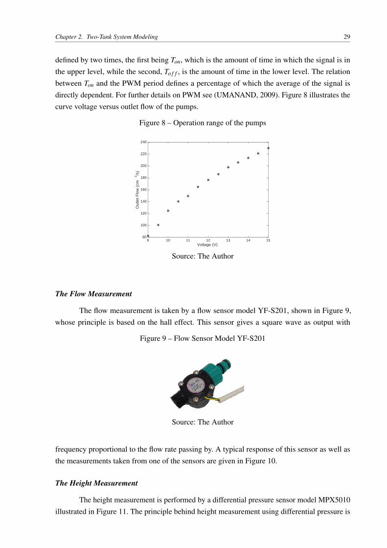
defined by two times, the first being Ton, which is the amount of time in which the signal is inthe upper level, while the second, To f f , is the amount of time in the lower level. The relationbetween Ton and the PWM period defines a percentage of which the average of the signal isdirectly dependent. For further details on PWM see (UMANAND, 2009). Figure 8 illustrates thecurve voltage versus outlet flow of the pumps.
Figure 8 – Operation range of the pumps
9 10 11 12 13 14 15Voltage (V)
80
100
120
140
160
180
200
220
240O
utle
t Flo
w (
cm3/s
)
Source: The Author
The Flow Measurement
The flow measurement is taken by a flow sensor model YF-S201, shown in Figure 9,whose principle is based on the hall effect. This sensor gives a square wave as output with
Figure 9 – Flow Sensor Model YF-S201
Source: The Author
frequency proportional to the flow rate passing by. A typical response of this sensor as well asthe measurements taken from one of the sensors are given in Figure 10.
The Height Measurement
The height measurement is performed by a differential pressure sensor model MPX5010illustrated in Figure 11. The principle behind height measurement using differential pressure is

Chapter 2. Two-Tank System Modeling 30
Figure 10 – Output of the flow sensors
10 20 30 40 50 60 70 80 90 100 110Frequency (Hz)
0
50
100
150
200
250
Flo
w r
ate
(cm
3/s
)
TypicalMeasured S1
Source: The Author
Figure 11 – Differential pressure sensor
Source: The Author
the fact that independently of the object’s shape the pressure is given by (HALLIDAY; RESNICK;WALKER, 2013):
∆P = ρgh (2.18)
where ∆P is the differential pressure, ρ is the specific weight of the liquid, g is the gravitationalacceleration and h is the liquid’s height. If g, ρ and P are known then the height h is found fromEq. 2.18 accordingly. Both Earth’s gravitational acceleration and water’s specific weight areknown, while the sensor gives the differential pressure. This makes possible the liquid’s heightmeasurement in the tanks. The sensor gives a linear voltage output according to the pressurelevel. Figure 12 shows a typical pressure versus voltage curve of a MPX5010 and an actual curveof both sensors (Tanks 1 and 2). The real curve was obtained as the average of ten experiments.The calibration was done using a ruler to measure the real liquid height.
The Valve Opening Measurement
The valve between the two-tank system can only be operated manually. The position ofthis valve changes the system behavior, and because of that it is important to measure the valve’sposition. This is done by an auxiliary system based on a potentiometer connected to the valve.

Chapter 2. Two-Tank System Modeling 31
Figure 12 – Curve voltage versus differential pressures
0 1 2 3 4 5 6Diferrential Pressure (KPa)
0
0.5
1
1.5
2
2.5
3
Out
put V
olta
ge (
V)
typicalS1S2
Source: The Author
Every time that the valve changes its position the resistance of the potentiometer also changes.Thus, a voltage divider is used to measure the valve’s aperture. It is important to notice that thismethod can only map the percentage of the valve’s aperture when the minimal and maximumvoltage are known. Figure 13 illustrates the real system.
Figure 13 – Valve’s aperture measurement
Source: The Author
2.6 The Experimental setup
As mentioned previously, in order to estimate the constant k for each valve, it is neces-sary to perform dedicated experiments. In this section these experiments will be the focus ofdiscussion.
The experiment to estimate the value of k is performed in the following way: for eachknown flow rate of the pump, the height of equilibrium is measured after a long period, enough forthe system to reach its steady state. It is known through Bernoulli’s equation that the equilibriumwater height and the flow rate of the pump are related as pointed in Eq. 2.6. This process is

Chapter 2. Two-Tank System Modeling 32
accomplished for both exit valves of each tank. For such experiment, a data set
q j,h jN
j=1 willbe collected, and based on it the value of k can be estimated .
Table 2 and 3 show, respectively, the data set collected from the experiment using thevalves from Tank 1 and 2. Each k from both valves were estimated using the Least Squares (LS)algorithm. See Sec. 3.4 for further details.
Table 2 – Data set from Tank 1’s valve
Flow (cm3/s) 216.2 202.6 192.1 186.8 176.3 165.8 157.4 149 141.7 133.3Height (cm) 51.5 44.5 38.5 34.5 30 24.5 20 15 12.5 9.5
Source: The Author
Table 3 – Data set from Tank 2’s valve
Flow (cm3/s) 220.4 209.9 199.4 190 180.5 170 159.5 150.1 139.6 129.1Height (cm) 55 48.5 43 37.5 32.5 28 22 17 12.5 9
Source: The Author
2.7 Summary of the Chapter
In this chapter, the nonlinear dynamic model for the TTS was derived according to themass balance principle. This model will be useful as a data generator for LPV identificationpurposes. The parameters of the TTS model depends on its geometrical shape. The measurementand actuator systems were described and an experimental procedure to obtain the value of theconstant k was given.
33
3 THE LINEAR PARAMETER-VARYING SYSTEM IDENTIFICATION
In this chapter are shown the methods used to identify models in the framework of LinearParameter-Varying (LPV) systems. In order to understand the dynamic behavior and what anLPV system is, it will be first described the basic properties of LPV systems in section 3.1,i.e.,its input-output relationship in association with the scheduling signal. In this context will bepresented the model structures of LPV systems in section 3.2, such as input-output (IO) andstate space(SS) representation. Following, methods to parametrically estimate these models areexamined in sections 3.3-3.5. In sequence, it will be shown a non-parametric strategy to estimateLPV Models in an input-output setting in section 3.6. An extension of the previous method thatdelivers unbiased estimates regardless of the noise structure is given in section 3.7.
3.1 LPV Systems
The LPV system framework was originally introduced by Shamma (1988). The idea wasto extend the gain-scheduling technique (ÅSTRÖM; WITTENMARK, 1994), which is a designapproach that constructs nonlinear controllers considering a nonlinear plant as an array of linearplants in many operational conditions. In the LPV framework, the so-called scheduling variablep, usually an external signal, plays an important role, it represents a dynamic mapping betweeninput u and output y. In this way, both have parameters that are p-dependent. As a matter of fact,LPV systems can describe both nonlinear behavior and time-varying phenomena, while keepingthe attractive structure of a linear system. In fact, for a constant signal p an LPV system behavesexactly as an LTI system. Regarding the LTI system theory, an LPV system can be seen as acollection of LTI systems interpolated by a scheduling function (based on p).
The LPV systems can be represented as a convolution depending on u and p, which indiscrete time is represented as (TÓTH, 2010):
y(k) =∞
∑i=0
gi(p)q−iu(k) , (3.1)
where q denotes the forward/backward time shift operator, i.e. q−iu(k) = u(k− i), u : Z→ Rnu
is the discrete input, y : Z→ Rny is the discrete output, and p : Z→ P is the scheduling variableof the system with scheduling space P⊆ Rnp . The coefficients gi in Eq. 3.1 are functions of thescheduling variable and they define the varying dynamical relation between u and y (TÓTH,2010). Additionally, there are two types of dependence related to time on p: the static anddynamic dependence. The former is when the coefficients gi depend only on instantaneous valuesof p, i.e. y(k) = g0(p(k))u(k)+g1(p(k))u(k−1)..., whereas the latter is defined by coefficientsthat depend on time-shifted versions of p, i.e. y(k) = g0(p(k), p(k− 1))u(k)+ g1(p(k), p(k−1), p(k−2))u(k−1).... As pointed out previously, for a constant p the convolution form of an

Chapter 3. The Linear Parameter-Varying System Identification 34
LPV system described by Eq. 3.1 is equivalent to an LTI system, where the coefficients gi areconstants. See (OPPENHEIM; WILLSKY; HAMID, 1996) for the definition of convolution inLTI systems. Figure 14 shows the relationship between aforementioned variables.
Figure 14 – LPV System
y(k)u(k)
p(k)
LPV
Source: The Author
3.2 LPV Model Structures
There are two basic types for LPV model representation: the IO and SS structures. Theseare based on the well-established LTI framework, see (OPPENHEIM; WILLSKY; HAMID,1996) for details. Again, the similarity between LPV and LTI systems are advantageous in termsof application. The equivalence between model structures IO and SS in the LPV frameworkis, in general, more complicated than the LTI counterpart, as in the LPV case usually involvesdynamic dependence on the scheduling variable(TÓTH, 2010). In this thesis, it will be exploredthe LPV-IO representation. Although the SS structure allows the insertion of noise in the model,the IO setting allows a clear separation between process and noise structures. In this way, IOrepresentation gives a better understanding of the model stochastic properties. Moreover, the IOrepresentation is relatively easier to parametrize and doesn’t suffer from explosions of data (curseof dimensionality), contrary to the SS representation (VAN WINGERDEN; VERHAEGEN,2009).
The LPV-IO Representation
This particular representation originates from the difference equation (discrete time)and is well-established in the LTI framework (OPPENHEIM; WILLSKY; HAMID, 1996). TheLPV-IO representation describes the system input-output behavior by using polynomial equationsin terms of the forward/backward time-shift operator. The model is generally described in a filterform:
y(k) =−na
∑i=1
ai(p)q−iy(k)+nb
∑j=0
b j(p)q− ju(k) , (3.2)
where the coefficients ainai=1 ,
b jnb
j=0 are the parameters of the model, which are functions ofthe scheduling p, with na ≥ 0 and nb ≥ 0. The model represented by Eq. 3.2 is usually referred asprocess model. As mentioned previously, these coefficients are considered with static dependence

Chapter 3. The Linear Parameter-Varying System Identification 35
on p. The case where na = 0, meaning that there is no output dynamic involved is known asFinite Impulse Response (FIR) model.
Usually in real world applications, the model represented in Eq. 3.2 is just an abstractionof the deterministic behavior of the system and, in general, it can barely represent the systembehavior. Therefore, a noise must be regarded in order to take into account uncertainties of thesystem. Typically, the noise added is white noise or a filtered version of it. Hence, the model inEq. 3.2 is described as following:
y(k) =−na
∑i=1
ai(p)q−iy(k)+q−nknb
∑j=0
b j(p)q− ju(k)+ e(k) , (3.3)
where e(k) is a zero-mean white noise process and nk is the dead time. This model is the LPVversion of the well-known ARX (Autoregressive with exogenous input) model from the LTIframework. Such model is part of a more general transfer function family. See (LJUNG, 1999)for further details on the LTI models.
The LPV-SS Representation
Similar to the LTI case, the LPV models have a state space representation, see (OPPEN-HEIM; WILLSKY; HAMID, 1996) for more details on LTI-SS structure. An LPV-SS model isgenerally described as:
qx = A(p)x+B(p)u ,
y =C(p)x+D(p)u ,
(3.4a)
(3.4b)
where x : Z→ Rnx is the state-variable and(A(p) ∈ Rnx×nx , B(p) ∈ Rnx×nu , C(p) ∈ Rny×nx ,
D(p) ∈ Rny×nu)
are matrix functions with static dependence on p. In the LPV framework, mostof the control synthesis assumes a state space representation as model.
3.3 LPV Identification Approaches
The first difference on the identification procedure of LPV systems is the necessity tomeasure a third signal entity, which is the scheduling variable. Usually for identification of LTIsystems, a data set in the form uk,ykN
k=1 must be collected, whereas in the LPV frameworkthis data set must include the scheduling variable. Hence, the data set must be in the form
DN = uk,yk, pkNk=1 . (3.5)
Basically, there are two approaches for identification of LPV systems: the local and globalapproaches. The former is based on the concept of LPV systems viewed as a collection of localLTI systems in an operational space. Whereas in the latter, data collection is done with a varyingp, ranging possibly all feasible scheduling space in order to provide a unique global model. Theprocedure in the local approach is to estimate LTI models from several working points. This
Chapter 3. The Linear Parameter-Varying System Identification 36
can be achieved by maintaining a constant p while collecting the data. Recall that for a constantscheduling p(k) = p for any k the LPV model is equivalent to an LTI model. Subsequently, theLPV system is obtained by an interpolation method, such as polynomial, radial basis functions,sigmoidal (TÓTH, 2010). When it comes to the global approach, a unique global structureassumption in the model within the scheduling space is considered, conversely of the localapproach. However, the estimation problem using a local approach can be solved similar to theglobal approach, by considering only one data set ranging many sub-data sets in many workingpoints. In (NOGUEIRA, 2012) was shown a local estimation approach using a global structure.One main drawback of this approach is the explosion of data (curse of dimensionality) as manyworking points are added. Such issue is unlikely to happen within the scope of a global approach,because of the global nature of the data collection.
In this thesis, it will be explored the methods within the scope of the global approachunder the LPV-IO setting.
3.4 The Regression Approach
The regression approach is based on considering the one-step ahead predictor of thesystem model in regression form. This method lies on the prediction error method (PEM)(LJUNG, 1999), which includes the maximum likelihood method, as well. In order to extend thePEM for LPV systems, it is necessary to define the concept of LPV system description. Then, itis possible to obtain a general one-step-ahead predictor to formulate the identification under themean-square error framework (MOHAMMADPOUR; SCHERER, 2012).
General LPV System Description
The general LPV system description can be extended from the LTI framework as aprocess filter with additive disturbance as:
y(k) = G(q, p)u(k)+ v(k), (3.6)
where G(q, p) is a p−dependent filter defined similarly as in Eq. 3.1. In (TÓTH, 2010) it wasshown that this filter can be equivalently defined as a convolution between u and p. This definitionis the LPV form of the impulse response (IR) in the LTI framework, where each gi(p) is the LPVequivalent of the impulse response coefficients. It is assumed that v is a quasi-stationary noiseprocess with a bounded power spectral density Φv(ω), and can be described by the followingrelationship:
v(k) = H(q, p)e(k), (3.7)
where H is a monic LPV filter as in Eq. 3.1. Similar to the LTI case, the filter H must beasymptotically stable in order for the identification problem to be well-posed under the predictionerror (PE) setting, see (MOHAMMADPOUR; SCHERER, 2012; LJUNG, 1999). Figure 15describes the signal flow of the general LPV system descriptor.

Chapter 3. The Linear Parameter-Varying System Identification 37
Figure 15 – Signal flow of the general LPV system descriptor
u(k) G(q, p)
p(k)
++
y(k)
H(q,p)
e(k)Source: The Author
General Assumptions Under LPV Identification Framework
A first assumption of the LPV framework stands the fact that the scheduling variablemust be a measurable entity. Another common assumption in literature involving the schedulingvariable is that measurements of p are noise free, see (BAMIEH; GIARRÉ, 2002; DANKERSet al., 2011; LOPES DOS SANTOS; RAMOS; MARTINS DE CARVALHO, 2007; LOPESDOS SANTOS et al., 2013; LAURAIN et al., 2011c; LAURAIN et al., 2012; LAURAIN et al.,2010a; TÓTH et al., 2011; LAURAIN et al., 2010b), exceptions are (BUTCHER; KARIMI;LONGCHAMP, 2008; PIGA et al., 2015; ABBASI et al., 2014). The main reason for theassumption of the noise free observations of the scheduling variable lies on issues regardingthe conditional expectation of v(k) when the true observation of p is not available, as eachcoefficient of the filter defined in Eq. 3.7 can be a nonlinear function with dynamic dependenceon p (MOHAMMADPOUR; SCHERER, 2012). This is a quite non-realistic scenario since,generally, observations of the scheduling variable are subject to uncertainties, such as, noisemeasurements due to sensors and experimental conditions.
In this thesis, it will be considered the case where true p, which is the noise-free versionof the scheduling variable, is available.
The One-Step Ahead Prediction of v
In order to formulate the estimation of parametric LPV models in the PE setting, it isnecessary to characterize the one-step ahead predictor of y (MOHAMMADPOUR; SCHERER,2012). Consequently, a one-step ahead prediction of the noise process is necessary to formu-late the prediction error. To do so, the filter H(q, p) must be stable and it must have a stableinverse, which means that, there exists a monic convergent filter denoted as H†(q, p) such that(H†(q, p)H(q, p)
)= 1 (TÓTH, 2010). This implies that Eq. 3.7 can be rewritten as:
e(k) = H†(q, p)v(k), (3.8)

Chapter 3. The Linear Parameter-Varying System Identification 38
and similarly to the LTI case, it can be shown that the one-step ahead predictor of v(k) is thefollowing (TÓTH, 2010):
v(k|k−1) =(
1−H†(q, p))
v(k). (3.9)
The One-Step Ahead Prediction of y
To address the problem of estimation parametric LPV models minimizing the predictionerror, which is the difference between the actual output and the predicted model output, it isnecessary to define the one-step ahead predictor of the model output y.
As an extension of the LTI case (LJUNG, 1999), it was shown that under the p true casewith information about yk−1 = y(τ)
τ≤k−1, uk = u(τ)τ≤k, and pk = p(τ)
τ≤k, the one-stepahead output predictor is (TÓTH, 2010):
y(k|k−1) =(
H†(q, p)G(q, p))
u(k)+(
1−H†(q, p))
y(k). (3.10)
Parametrization of LPV Models
In order to write the LPV-IO model in the regression, the scheduling variable dependen-cies must be well-defined. The main requirement is that the model must be linear in parameters.To parametrize the model it will be considered that each parameter of the filter A(p) and B(p)
can be decomposed in terms of a priori selected basis set ψi j : P→ R. Then for i = 1, ...na eachelement of A(p) in Eq. 3.2 can be defined as:
ai(p(k)) = θi0 +θi1ψi1(p(k))+ · · ·+θilψisi(p(k)), (3.11)
where θi j ∈ R are the unknown parameters to be identified. Similarly, each element of B(p) inEq. 3.2 can be defined for i = 0, ...nb as:
bi(p(k)) = θi0 +θi1ψi1(p(k))+ · · ·+θilψisi(p(k)). (3.12)
It is possible to select a function φ(·) that generalizes the dependency on p(k) for each parameterof the LPV-IO model. In this way, the process part is fully characterized by φi(·)na+nb+1
i=1 .Therefore, the LPV model in a regression form must be linearly parametrized as follows:
φi(·) = θi0 +si
∑j=1
θi jψi j(·), (3.13)
once this parametrization is chosen, it becomes possible to pose the estimation problem in aregression form. As pointed in (BAMIEH; GIARRÉ, 2002) there are many possibilities forthe choice of the basis functions, such as, monomials, periodic functions like sine and cosine,and sigmoidal. It is a common assumption in literature that this parameter dependency is ofpolynomial form, see (BAMIEH; GIARRÉ, 2002; BUTCHER; KARIMI; LONGCHAMP, 2008;LAURAIN et al., 2010b). This corresponds to the following parametrization:
ψi, j(p(k)) = p j(k). (3.14)

Chapter 3. The Linear Parameter-Varying System Identification 39
MIMO LPV-IO Models
In this thesis, it will be dealt mainly with multiple inputs multiple outputs (MIMO)systems. For this reason, a formal characterization of these models in an IO setting is necessary.The extension to MIMO LPV-IO is accomplished similarly for the LTI case (LJUNG, 1999). TheMIMO LTI-ARX model can be described as in Eq. 3.3 by analogy (LJUNG, 1999):
y(k) =−na
∑i=1
AAAiq−iy(k)+nb
∑j=0
BBB jq−nk− ju(k)+ e(k), (3.15)
with y ∈ Rny the vector output, u ∈ Rnu the vector input, and the coefficient matrices Ai, B j
defined as:
y(k) =[y1(k) · · ·yny(k)
]T, u(k) = [u1(k) · · ·unu(k)]
T , (3.16)
AAAi =
ai,1,1 · · · ai,1,ny
... . . . ...ai,ny,1 · · · ai,ny,ny
, BBB j =
bi,1,1 · · · bi,1,nu
... . . . ...bi,ny,1 · · · bi,ny,nu
, (3.17)
where e(k) =[e1(k) · · ·eny(k)
]T is a white noise stochastic vector. However, this model assumesthat each output channel has influence over each other, leading to dynamics of each outputinfluencing each other. A common approach in dealing with MIMO systems is to assume thatthere is no influence in dynamics from other outputs. In this way, the matrix AAAi in Eq. 3.17assumes the following form:
AAAi =
ai,1 · · · 0
... . . . ...0 · · · ai,ny
, (3.18)
Using this parametrization, identification of a MIMO LTI system can be performed separatelyfor each output via the estimation of multiple input single output (MISO) systems (LJUNG,1999). In fact, it is preferable to cope with the estimation of ny MISO systems than a MIMOsystem, mainly to avoid overparametrization due to the presence of zeros on the regressors. Toextend this model to the LPV-ARX case it is just necessary to allow the coefficients in matricesto depend on p, by using the LPV matrices AAAi(p(k)) and BBB j(p(k)):
AAAi(p(k)) =
ai,1,1(p(k)) · · · 0
... . . . ...0 · · · ai,ny,ny(p(k))
,BBB j(p(k)) =
bi,1,1(p(k)) · · · bi,1,nu(p(k))
... . . . ...bi,ny,1(p(k)) · · · bi,ny,nu(p(k))
,
(3.19)
with the following equation defining the MISO LPV-ARX Model:
y(k) =na
∑i=1
AAAi(p(k))q−iy(k)+nb
∑j=0
BBB j(p(k))q−nk− ju(k). (3.20)

Chapter 3. The Linear Parameter-Varying System Identification 40
Where y(k) is a scalar corresponding to one specific output of the MIMO system, u(k) is definedin Eq.3.16 and AAAi, BBB j are defined as in Eq.3.19. In the case of the MIMO LPV-ARX system, theset
φi, jny,nt
i=1; j=1 fully characterizes the dependence on the scheduling variable, with each basisfunction as in Eq. 3.13:
φi, j(·) = θi, j,0 +si j
∑k=1
θi, j,kψi, j,k(·), (3.21)
with nt = na +nu (nb +1), and each φi, j is a real function with static dependence on p(k).
Estimation via the LS Criterion
It is possible to write the LPV-IO model as a linear regression form using Eqs. 3.3 and3.13. Firstly, it is necessary to write the LPV model in a linear regression form as:
y(k) = ϕT (k)θ + e(k), (3.22)
where y is the output, ϕ is the regression vector, θ is the parameter of the model and e is agaussian white noise process. For the LPV-ARX model defined in Eq. 3.3, this transformationis straightforward. However, in order to write this model in regression form, it is first requiredto choose appropriate basis functions that properly parametrize the model in p as in Eq. 3.13.Choosing a linear in parameters basis function leads to coefficients of filter A and B in the formof Eqs. 3.11-3.12. Then, the parameter and regression vectors in Eq. 3.22 for the LPV-ARXmodel will be the following:
θT =
[θ10 · · ·θ1s1 θ20 · · ·θ2s2 · · ·θnasna
θna+10 · · ·θna+1sna+1 · · ·θngsng
]ϕ
T (k) =[− y(k−1) − y(k−1)ψi1(p(k)) · · ·− y(k−na)ψnasna
(p(k)) · · ·
u(k−nk) u(k−nk)ψna+11(p(k)) · · · u(k−nk−nb +1)ψngsng(p(k))
](3.23a)
(3.23b)
where ng = na+nb+1. The MISO LPV-ARX can be parametrized in a similar fashion. It is onlynecessary to add the additional inputs and their respective parameters in the regression equation.The only requirement is that the whole model must be linear in parameters. Then, the regressorsand the parameter vectors of the MISO LPV-ARX can be defined as follows:
θT =
[θ10 · · ·θ1s1 θ20 · · ·θ2s2 · · ·θnasna
θna+10 · · ·θna+1sna+1 · · ·θntsnt
]ϕ
T (k) =[− y(k−1) − y(k−1)ψi1(p(k)) · · ·− y(k−na)ψnasna
(p(k)) · · ·
u1(k−nk) u1(k−nk)ψ1,na+1,1(p(k)) · · · u1(k−nk−nb +1)ψ1,ng,sng(p(k)) · · ·
unu(k−nk) unu(k−nk)ψnu,na+1,1(p(k)) · · · unu(k−nk−nb +1)ψnu,ng,sng(p(k))
]
(3.24a)
(3.24b)
with the first index of θi, j,k, and ψi, j,k not used because there is only one output for MISOsystems. The Least Squares criteria is based on the minimization of the mean square error, whichis summarized in the following cost function:
VN =1N
N
∑i=1
e2(i), (3.25)

Chapter 3. The Linear Parameter-Varying System Identification 41
with the LS estimates as a minimizer defined as follows:
θLS = argminVN , (3.26)
it is well-known that for the linear regression case the minimum of Eq. 3.25 can be found asfollows, by defining YYY = [y(1) y(2) · · ·Y (N)]T and ΦΦΦ = [ϕ(1)ϕ(2) · · ·ϕ(N)]T (LJUNG, 1999):
θLS = ΦΦΦ†YYY , (3.27)
where ΦΦΦ† =
( 1N ΦΦΦ
TΦΦΦ)−1 1
N ΦΦΦT is the regularized version of the Penroe-Monrose pseudoinverse
(LJUNG, 1999; MOHAMMADPOUR; SCHERER, 2012). This solution is identical to the LTIcase (LJUNG, 1999), which is possible because an LPV system can be viewed as a multipleinput single output (MISO) LTI model with virtual inputs as pointed in (MOHAMMADPOUR;SCHERER, 2012; LAURAIN et al., 2010a; LAURAIN et al., 2010b). However, it is well-known that the minimizer in Eq. 3.27 leads to an unbiased estimate if the noise e in Eq. 3.22 iswhite, which is only true for the ARX model structure (LJUNG, 1999; MOHAMMADPOUR;SCHERER, 2012).
Recursive Versions of the LS Algorithm
The adopted LS approach herein is based on the classical approach, which considers theregression vector stacked as column. As the LPV-ARX model can be viewed as an LTI MISOsystem, other type of parametrizations arise. In (BAMIEH; GIARRÉ, 2002) it was shown thatthe least mean squares (LMS) and recursive least squares (RLS) algorithms can be extended tothe LPV case. A parametrization similar to the MISO LTI models was chosen (LJUNG, 1999),where the regression and parameter vectors in Eqs. 3.23a, 3.23b are matrices, instead of vectors.
The parametrization is then performed in the following way. Define the parameter matrixΘΘΘ ∈ Rng×np , with np being the number of basis functions, as:
ΘΘΘ :=
a11 · · · anp
1
a12 · · · anp
2...
......
a1na· · · anp
na
b10 · · · bnp
0...
......
b1nb · · · bnp
nb
. (3.28)
Herein it will be considered the subscript as an indicator of sample, e.g. yk = y(k). Define the
Chapter 3. The Linear Parameter-Varying System Identification 42
extended regression matrix as:
ΨΨΨk := ϕkπk :=
−yk−1...
−yk−na
uk...
uk−nb
[ψ1(p(k)) ψ2(p(k)) · · ·ψnp(p(k))
], (3.29)
based on this, it is possible to infer that the model output of the LPV model is as follows:
yk =< ΘΘΘ,ΨΨΨk >, (3.30)
which is referred in (BAMIEH; GIARRÉ, 2002) as the notation of inner product, definedas < A,B >:= trace(A∗B) = trace(BA∗) with A and B matrices of same dimension and A∗
the transposed conjugate of matrix A. Also, the generalization of outer product is defined as(U⊗V )(X) :=U <V,X > with U ∈ Rn×m and V ∈ Rp×q and the outer product is an operator(U⊗V ) : Rp×q→ Rn×m, see (BAMIEH; GIARRÉ, 2002) for further details.
As Eq. 3.30 defines a linear relationship as in 3.22, it can be similarly solved using Eq.3.27. However, another approach will be taken in this work, instead of solving the cost functionanalytically, steps will be taken towards to the minimum of the mean square cost function in 3.25.To minimize the cost function iteratively the steepest descent strategy will be used for updatingthe parameters as follows:
δ ΘΘΘ = ΘΘΘk− ΘΘΘk−1 =−12
αg(ΘΘΘk−1), (3.31)
where g(ΘΘΘk−1) =dV (ΘΘΘ)
dΘΘΘis the mean square error gradient and α is the step size. An instantaneous
approximation of the cost function in Eq.3.25 is:
V (ΘΘΘ) = e(k,ΘΘΘ)2, (3.32)
which is the LMS equivalent. The updating of the parameters is done according to the followingrecursion:
ΘΘΘk+1 = ΘΘΘk−α
(ek
ddΘΘΘ
(yk− trace(ΘΘΘT
ΨΨΨk)))
= ΘΘΘk +αekΨΨΨk, (3.33)
recalling that ek = yk− trace(ΘΘΘTΨΨΨk) and the derivative property (d/dX)trace(XT B) = B. In
(BAMIEH; GIARRÉ, 2002) a recursive version of the LS algorithm was shown over a generalfinite dimensional inner product space, rather than the Euclidian space. This is done in orderto provide a proof on results related to the persistency of excitation condition. It was pointed

Chapter 3. The Linear Parameter-Varying System Identification 43
out that the RLS version in this inner product space is similar to the euclidean version (LJUNG,1999) and it has the following form:
ΘΘΘk = ΘΘΘk−1 +KKKkek
KKKk = PPPkΨΨΨk
PPPk = PPPk−1−PPPk−1ΨΨΨk⊗ΨΨΨk
1+< ΨΨΨk,PPPk−1ΨΨΨk >PPPk−1,
(3.34a)
(3.34b)
(3.34c)
it is worth to remind that these versions of LMS and RLS can be transformed on the usualform (LJUNG, 1999) by stacking the components of the extended regression matrix ΨΨΨ and theparameter matrix ΘΘΘ in a column vector as in Eqs. 3.23a, 3.23b.
3.5 The Correlation Approach
The correlation approach is based on a regression form as well. However, in this approach,it is not assumed that the noise stochastic process is white. In typical cases the θLS estimatedvia LS do not tend to the true model, giving an unbiased estimate. The reason is, typically, thecorrelation between v(k) and ϕ(k)(LJUNG, 1999). One alternative is to introduce a generalcorrelation vector ζ (k) in the least squares problem. In identification literature this method iscalled instrumental variable method (IVM), and ζ (k) the instruments. It’s required that theseinstruments must be derived from past data and they must be transformed in a certain way thatthey are uncorrelated with the prediction error sequence(LJUNG, 1999). Resulting in
1N
N
∑k=1
ζ (k)e(k,θ) = 0, (3.35)
the solution θIV that satisfies this equation gives the best estimate based on the observed dataand it is of the form:
θIV =
[1N
N
∑k=1
ζ (k)ϕT (k)
]−11N
N
∑k=1
ζ (k)y(k). (3.36)
A complete treatment of instrumental variable methods is given in (SÖDERSTRÖM; STOICA,1983). In this section, it will be shown how the instrumental variable method is extended to theLPV framework.
Instrumental Variable Method for LPV Systems
The IVM was introduced and its consistency analyzed in the LPV framework in (BUTCHER;KARIMI; LONGCHAMP, 2008). While in the LTI case, the instrumental vector ζ (k) dependson the regressors ϕ(k), in the LPV case, this instrumental vector also depends on the schedulingvariable p(k). As shown in (BUTCHER; KARIMI; LONGCHAMP, 2008) the consistency ofthe IVM depends on two conditions (Similar to the LS case):
E
ζ (k)ϕT (k)> 0 and Eζ (k)e(k)= 0, (3.37)
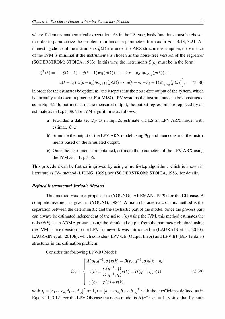
Chapter 3. The Linear Parameter-Varying System Identification 44
where E denotes mathematical expectation. As in the LS case, basis functions must be chosenin order to parametrize the problem in a linear in parameters form as in Eqs. 3.13, 3.21. Aninteresting choice of the instruments ζ (k) are, under the ARX structure assumption, the varianceof the IVM is minimal if the instruments is chosen as the noise-free version of the regressor(SÖDERSTRÖM; STOICA, 1983). In this way, the instruments ζ (k) must be in the form:
ζT (k) =
[− y(k−1) − y(k−1)ψi1(p(k)) · · ·− y(k−na)ψnasna
(p(k)) · · ·
u(k−nk) u(k−nk)ψna+11(p(k)) · · · u(k−nk−nb +1)ψngsng(p(k))
], (3.38)
in order for the estimates be optimum, and y represents the noise-free output of the system, whichis normally unknown in practice. For MISO LPV systems the instruments can be constructedas in Eq. 3.24b, but instead of the measured output, the output regressors are replaced by anestimate as in Eq. 3.38. The IVM algorithm is as follows:
a) Provided a data set DN as in Eq.3.5, estimate via LS an LPV-ARX model withestimate θLS;
b) Simulate the output of the LPV-ARX model using θLS and then construct the instru-ments based on the simulated output;
c) Once the instruments are obtained, estimate the parameters of the LPV-ARX usingthe IVM as in Eq. 3.36.
This procedure can be further improved by using a multi-step algorithm, which is known inliterature as IV4 method (LJUNG, 1999), see (SÖDERSTRÖM; STOICA, 1983) for details.
Refined Instrumental Variable Method
This method was first proposed in (YOUNG; JAKEMAN, 1979) for the LTI case. Acomplete treatment is given in (YOUNG, 1984). A main characteristic of this method is theseparation between the deterministic and the stochastic part of the model. Since the process partcan always be estimated independent of the noise v(k) using the IVM, this method estimates thenoise v(k) as an ARMA process using the simulated output from the parameter obtained usingthe IVM. The extension to the LPV framework was introduced in (LAURAIN et al., 2010a;LAURAIN et al., 2010b), which considers LPV-OE (Output Error) and LPV-BJ (Box Jenkins)structures in the estimation problem.
Consider the following LPV-BJ Model:
Sθ =
A(pk,q−1,ρ)χ(k) = B(pk,q−1,ρ)u(k−nk)
v(k) =C(q−1,η)
D(q−1,η)e(k) = H(q−1,η)e(k)
y(k) = χ(k)+ v(k),
(3.39)
with η = [c1 · · ·cncd1 · · ·dnd ]T and ρ = [a1 · · ·anab0 · · ·bnb]
T with the coefficients defined as inEqs. 3.11, 3.12. For the LPV-OE case the noise model is H(q−1,η) = 1. Notice that for both

Chapter 3. The Linear Parameter-Varying System Identification 45
LPV-OE and LPV-BJ structures, the scheduling variable p(k) only affects the process part. Basedon the PEM approach, it can be shown that the prediction error with respect to Eq. 3.39 is(LAURAIN et al., 2010b):
eθ (k) =D(q−1,η)
C(q−1,η)A†(pk,q−1,ρ)×
(A(pk,q−1,ρ)y(k)−B(pk,q−1,ρ)u(k)
), (3.40)
where D(q−1,η)/C(q−1,η) can be recognized as the inverse of the ARMA noise model. Al-though the prediction error of the LPV case is similar to the LTI case, the polynomial operatorsdo not commute. Hence, no filter can be chosen such that both conditions hold simultaneously(LAURAIN et al., 2010b):
A(pk,q−1,ρ)y f (k) =D(q−1,η)
C(q−1,η)A†(pk,q−1,ρ)A(pk,q−1,ρ)y(k),
B(pk,q−1,ρ)u f (k) =D(q−1,η)
C(q−1,η)A†(pk,q−1,ρ)B(pk,q−1,ρ)u(k),
(3.41a)
(3.41b)
which means that no filtering of data can lead a regression equation with a white noise process.In order to introduce a model which provides a solution the identification problem, rewrite thesignals’ relations in Eq. 3.39 as (LAURAIN et al., 2010b):
Sθ =
χ(k)+na
∑i=1
ai0χ(k− i)︸ ︷︷ ︸F(q−1)χ(k)
+na
∑i=1
nα
∑l=1
ail fl(pk)χ(k− i)︸ ︷︷ ︸χil(k)
=nb
∑j=0
nβ
∑l=0
b jl gl(pk)u(k−nk− j)︸ ︷︷ ︸u jl(k)
v(k) =C(q−1,η)
D(q−1,η)e(k) = H(q−1,η)e(k)
y(k) = χ(k)+ v(k),
(3.42)
here, it is assumed that each ai, i = 1, ...na has the same number of elements, that is, each ai
has nα elements in Eq.3.11. The same assumption is valid to the number of elements of eachb j, j = 1, ...nb, that is nβ . Also, the basis functions in Eqs. 3.11 and 3.12 are denoted by fl and gl ,with g0 = 1 and F(q−1) = 1+∑
nai=1 ai0q−i. In this form, the LPV-BJ represents a MISO system
with (nb+1)(nβ +1) inputs χilna,nα
i=1,l=1 and
u jlnb,nβ
j=0,l=0 with the scheme represented in Figure16.
Since now the operator commutes (there is no dependence on p(k)), Eq. 3.42 can berewritten as:
y(k) =−na
∑i=1
nα
∑l=1
ail
F(q−1)χil(k)+
nb
∑j=0
nβ
∑l=0
b jl
F(q−1)u jl(k)+H(q−1,η)e(k), (3.43)
which is an LTI interpretation of Eq. 3.42. Using Eq. 3.43, y(k) can now be written in theregression form as:
y(k) = ϕT (k)ρ + v(k), (3.44)

Chapter 3. The Linear Parameter-Varying System Identification 46
Figure 16 – MISO interpretation of an LPV system
Source: See (LAURAIN et al., 2010b)
where,
ϕT (k) =
[−y(k−1) · · ·− y(k−na) −χ11(k) · · ·−χnanα
(k) u00(k) · · ·unbnβ(k)]
ρT =
[a10 · · ·ana0 a11 · · ·ananα b00 · · ·bnbnβ
]v(k) = F(q−1,ρ)v(k).
(3.45a)
(3.45b)
(3.45c)
In the LPV-BJ MISO case, it is necessary to add a third index which refers to the k− th input. Inthis way, the regressors in Eq. 3.45a will also have elements of this type:
uk, j,l
nu,nb,nβ
k=1, j=0,l=0, whilethe parameters in Eq. 3.45b will have
bk, j,l
nu,nb,nβ
k=1, j=0,l=0. Now, based on the LTI representationin Eq. 3.43 the prediction error is given as:
eθ (k) =D(q−1,η)
C(q−1,η)F(q−1,ρ)
(F(q−1,ρ)y(k)+
na
∑i=1
nα
∑l=1
ailχil(k)−nb
∑j=0
nβ
∑l=0
b jlu jl(k)
), (3.46)
where D(q−1,η)/C(q−1,η) can be recognized again as the inverse of the ARMA noise model.However, since this system represents an LTI model (the polynomial operator commutes), theprediction error can be rewritten as:
F(q−1,ρ)y f (k)+na
∑i=1
nα
∑l=1
ailχf
il (k)−nb
∑j=0
nβ
∑l=0
b jlufjl(k), (3.47)
where y f (k), u fjl(k) and χ
fil (k) represent the outputs of the prefiltering operation, using the
following filter:
Q(q−1,θ) =D(q−1,η)
C(q−1,η)F(q−1,ρ). (3.48)

Chapter 3. The Linear Parameter-Varying System Identification 47
Based on Eq. 3.47, the associated linear in parameters model takes the form (YOUNG, 1984):
y(k) = ϕTf (k)ρ + v f (k), (3.49)
where,
ϕTf (k) =
[−y f (k−1) · · ·− y f (k−na) −χ
f11(k) · · ·−χ
fnanα
(k) u f00(k) · · ·u
fnbnβ
(k)]
v f (k) = F(q−1,ρ)v f (k)
= F(q−1,ρ)D(q−1,η)
C(q−1,η)F(q−1,ρ)v(k) = e(k),
(3.50a)
(3.50b)
this result means that the stochastic part of the regression in Eq. 3.49 is equivalent to a white noiseprocess as pointed in Eq. 3.50b. Hence, the optimal solution can be obtained by the LS approach.However, the filter in Eq.3.48 is usually not known a priori. The RIV algorithm is then basedon two main steps. First, a reliable estimate of ρ must be used in the presence of colored noise.The main alternative is the use of the IVM as pointed in (YOUNG, 1984), (SÖDERSTRÖM;STOICA, 1983). Second, after obtained a reliable estimate of the process part, the predictionerror can be obtained using the simulation output of the model previously estimated. In this waythe filter in Eq. 3.49 can be estimated by using an algorithm that estimates ARMA processes,like the same IVM as pointed in (YOUNG, 1984). For the LPV-BJ case, the RIV algorithm is asfollows (LAURAIN et al., 2010b):
a) Based on a data set as in Eq. 3.5, estimate an LPV-ARX model using the LS approachand denote by θ0 its estimate. Assume that η is some initial value. Set τ = 0;
b) Compute an estimate of χ(k) via A(p(k),q−1, ρ(τ))χ(k) = B(p(k),q−1, ρ(τ))u(k−nk), where ρ(τ) is estimated in the previous iteration. Based on Eq. 3.42, deduceχil(k)na,nα
i=1,l=0.
c) Compute the estimated filter:
Q(q−1,θ) =D(q−1,η)
C(q−1,η)F(q−1,ρ),
and the associated filtered signals y f (k), χ fil (k)
na,nα
i=1,l=0 and u fjl
nb,nβ
j=0,l=0;
d) Build the filtered estimated regressor ϕ f (k) and the filtered instruments ζ f (k) as:
ϕTf (k) =
[−y f (k−1) · · ·− y f (k−na) − χ
f11(k) · · ·− χ
fnanα
(k) u f00(k) · · ·u
fnbnβ
(k)]
ζTf (k) =
[−χ f (k−1) · · ·− χ f (k−na) − χ
f11(k) · · ·− χ
fnanα
(k) u f00(k) · · ·u
fnbnβ
(k);]
e) Now solve the IVM as:
ρ(τ+1) =
[N
∑k=1
ζ f (k)ϕTf (k)
]−1 N
∑k=1
ζ f (k)y f (k);

Chapter 3. The Linear Parameter-Varying System Identification 48
f) obtain an estimate of the noise signal v(k) as:
v(k) = y(k)− χ(k, ρ(τ));
based on v the estimation of the noise parameter vector η(τ+1) follows; if θ (τ+1) hasconverged or the maximum number of iterations is reached, then stop, else increase τ
by 1 and go back to item b) and repeat the procedure.
This procedure can be used for LPV-OE models, being only necessary to skip item f), since theLPV-OE structure does not assume an ARMA filter on the noise model. This algorithm receivesthe name of simplified refined instrumental variable (SRIV) algorithm (LAURAIN et al., 2010a;LAURAIN et al., 2010b; YOUNG, 1984).
3.6 The LS-SVM approach
The methods presented so far depend on an additional user choice, the adequate selectionof the basis functions ψ in Eq. 3.13 to parametrize the LPV model. Besides the inherentidentification questions like, the polynomial orders na, nb, nk. The basis set selection is ofparamount importance for the identification task. Generally, in order to capture the underlyingdependence of ai and b j on p, which can range from simple polynomial to rational and evendiscontinuous functions, a large set of basis is adopted. However, in many cases, only a fewmight be needed for an accurate approximation. This means that methods which were shownpreviously may face an over-parametrization problem (TÓTH et al., 2011). As a solution to thisproblem, a support vector machine (SVM) approach was introduced in (TÓTH et al., 2011). Inthis section, it will be presented how the LPV-IO can be modeled in the LS-SVM frameworkand how to identify the feature map involved with the unknown dependence on the schedulingvariable.
Support Vector Machines
The SVMs were originally introduced by Valpnik and they have their roots on statisticallearning theory (VAPNIK, 1999). The original SVM aims to separate two classes in the bestpossible way. The best solution in the SVM framework is related to the margin concept, whichplays an important role in the SVM theory. To illustrate the problem which the SVM wasintroduced to solve, consider the case in Figure 17, where there are two classes. The problemhere is to find a linear classifier ωT x+ b that is able to solve the separation problem, that is,capable of classifying correctly the two classes. An optimal classifier will separate the mappeddata set by the highest margin, which can be shown that is equivalent to 2/||ω||2 (VAPNIK, 1999;SCHÖLKOPF; SMOLA, 2002; SUYKENS; VAN GESTEL; DE BRABANTER, 2002). Thus,the optimal classifier can be achieved with the maximization of the margin, but notice that thisis equivalent to the minimization of ||ω|| subject to the correct classification yk
[ωT x+b
]≥ 1
with yk ∈ R labeled as yk ∈ −1,1. Although this form of SVM can solve many problems,
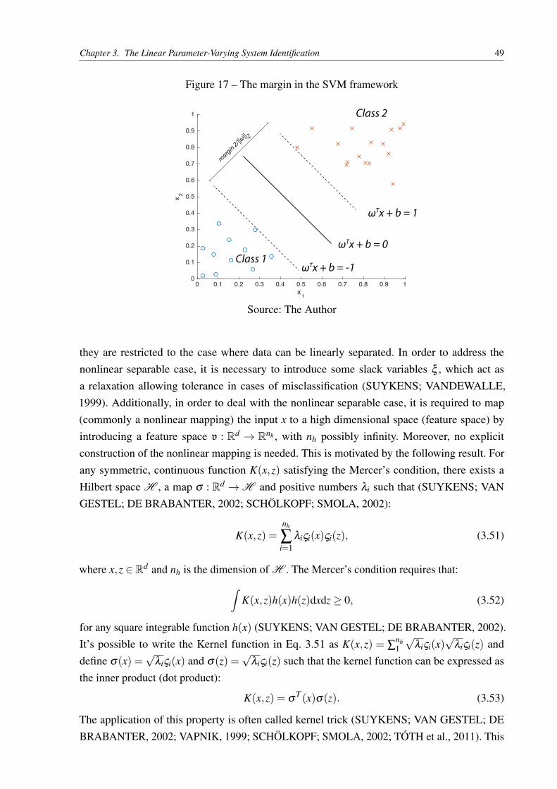
Chapter 3. The Linear Parameter-Varying System Identification 49
Figure 17 – The margin in the SVM framework
0 0.1 0.2 0.3 0.4 0.5 0.6 0.7 0.8 0.9 1x
1
0
0.1
0.2
0.3
0.4
0.5
0.6
0.7
0.8
0.9
1
x2
Class 2
Class 1
ωTx + b = 1
ωTx + b = 0
ωTx + b = -1
margin 2/||ω|| 2
Source: The Author
they are restricted to the case where data can be linearly separated. In order to address thenonlinear separable case, it is necessary to introduce some slack variables ξ , which act asa relaxation allowing tolerance in cases of misclassification (SUYKENS; VANDEWALLE,1999). Additionally, in order to deal with the nonlinear separable case, it is required to map(commonly a nonlinear mapping) the input x to a high dimensional space (feature space) byintroducing a feature space v : Rd → Rnh , with nh possibly infinity. Moreover, no explicitconstruction of the nonlinear mapping is needed. This is motivated by the following result. Forany symmetric, continuous function K(x,z) satisfying the Mercer’s condition, there exists aHilbert space H , a map σ : Rd →H and positive numbers λi such that (SUYKENS; VANGESTEL; DE BRABANTER, 2002; SCHÖLKOPF; SMOLA, 2002):
K(x,z) =nh
∑i=1
λiςi(x)ςi(z), (3.51)
where x,z ∈ Rd and nh is the dimension of H . The Mercer’s condition requires that:∫K(x,z)h(x)h(z)dxdz≥ 0, (3.52)
for any square integrable function h(x) (SUYKENS; VAN GESTEL; DE BRABANTER, 2002).It’s possible to write the Kernel function in Eq. 3.51 as K(x,z) = ∑
nh1√
λiςi(x)√
λiςi(z) anddefine σ(x) =
√λiςi(x) and σ(z) =
√λiςi(z) such that the kernel function can be expressed as
the inner product (dot product):
K(x,z) = σT (x)σ(z). (3.53)
The application of this property is often called kernel trick (SUYKENS; VAN GESTEL; DEBRABANTER, 2002; VAPNIK, 1999; SCHÖLKOPF; SMOLA, 2002; TÓTH et al., 2011). This
Chapter 3. The Linear Parameter-Varying System Identification 50
strategy allows one to work in the feature space without having to make computations on thatspace. The problem then becomes (SUYKENS; VAN GESTEL; DE BRABANTER, 2002):
minω,b,ξ
JP(ω,ξ ) =12
ωT
ω + cN
∑k=1
ξk
such that yk[ω
Tv(xk)+b]≥ 1−ξk, k = 1, ...N,
ξk ≥ 0, k = 1, ...N,
(3.54)
where c is a positive constant. The optimization problem in Eq. 3.54 is usually called the primalform of the SVM. The Lagragian for this problem is:
L (ω,b,ξ ;α,ν) = J(ω,ξ )−N
∑k=1
αk(yk[ω
Tv(xk)+b]−1+ξk
)−
N
∑k=1
νkξk, (3.55)
with the Lagrangian multipliers αk ≥ 0,νk ≥ 0 for k = 1, ...,N. The optimal solution of thisproblem can be obtained at the saddle point of the Lagragian (SUYKENS; VAN GESTEL; DEBRABANTER, 2002):
maxα,ν
minω,b,ξ
L (ω,b,ξ ;α,ν). (3.56)
Then, it is possible to eliminate the primal variables by setting the partial derivatives of theLagrangian with respect to the primal variable ω,b,ξk to be equal to zero:
∂L
∂ω= 0→ ω =
N
∑k=1
αkykv(xk)
∂L
∂b= 0→
N
∑k=1
αkyk = 0
∂L
∂ξk= 0→ 0≤ αk ≤ c, k = 1, . . . ,N.
(3.57a)
(3.57b)
(3.57c)
Finally, the dual problem of the SVM can be posed as:
maxα
JD(α) =− 12
N
∑k,l=1
ykyl vT (xk)v(xl)︸ ︷︷ ︸
K(xk,xl)
αkαl +N
∑k=1
αk
such thatN
∑k=1
αkyk = 0; 0≤ αk ≤ c, k = 1, . . . ,N.
(3.58)
The dual problem is more attractive to the LPV identification due to the fact that it is onlynecessary to define a type of kernel, instead of characterizing the explicit dependencies of thenonlinear mapping. Moreover, in this form, it is possible to formulate the problem withoutexplicitly describing the parameter vector ω .
Leasts Squares Support Vector Machines
The formulation in Eq. 3.58 defines a quadratic programming (QP) problem. Althoughthis formulation leads to a convex optimization problem and to sparseness on the solution, it is

Chapter 3. The Linear Parameter-Varying System Identification 51
generally more complicated to solve than a simple LS problem. Motived by that, in (SUYKENS;VANDEWALLE, 1999) was proposed a modification in the original SVM problem in order tosimplify its solution. The QP problem was transformed in a linear regression problem with ananalytic solution. This method was called least squares support vector machine (LS-SVM). TheLS-SVM problem is written as:
minω,b,e
JP(ω,b,e) =12
ωT
ω +γ
2
N
∑k=1
e2k
such that yk[ω
Tv(xk)+b]= 1− ek, k = 1, . . . ,N.
(3.59)
This formulation modifies the original SVM problem in two aspects. The first one is, insteadof the inequality constraints used in the original SVM, it is used equality constraints where thevalue of the right hand side is considered as a target rather than a threshold value. As in theoriginal SVM case, an error variable e is introduced to play a similar role of the slack variablesand allow misclassifications. Second, a squared loss function is taken for this error variable(SUYKENS; VAN GESTEL; DE BRABANTER, 2002). As in the original SVM, it is possibleto derive the problem in the dual form using the Lagrangian once again as:
L (ω,b,e;α) = J(ω,b,e)−N
∑k=1
αk(yk[ω
Tv(xk)+b]−1+ ek
), (3.60)
where αk are the Lagrangian multipliers, which can be either positives or negatives due to theequality constraints. The Karush-Kuhn-Tucker (KKT) conditions for optimality yield:
∂L
∂ω= 0→ ω =
N
∑k=1
αkykv(xk)
∂L
∂b= 0→
N
∑k=1
αkyk = 0
∂L
∂ek= 0→ αk = γek, k = 1, . . . ,N
∂L
∂αk= 0→ yk
[ω
Tv(xk)+b]−1+ ek = 0, k = 1, . . . ,N.
(3.61a)
(3.61b)
(3.61c)
(3.61d)
The value of α and b can be obtained by formulating a linear KKT system as:[0 yT
y Ω+ I/γ
][b
α
]=
[0
1v
], (3.62)
where y = [y1 . . . yN ]T , 1v = [1 . . . 1]T , e = [e1 . . . eN ]
T , α = [α1 . . . αN ]T . The variable Ω is
known as the kernel matrix and is defined as (SUYKENS; VAN GESTEL; DE BRABANTER,2002):
Ωkl = ykylvT (xk)v(xl)
= ykylK(xk,xl), k = 1, . . . ,N.
(3.63)
Although the LS-SVM offers a unique and global solution, a main drawback related to theoriginal SVM is the lack of sparseness (SUYKENS; VAN GESTEL; DE BRABANTER, 2002).

Chapter 3. The Linear Parameter-Varying System Identification 52
LPV formulation in the LS-SVM Setting
The extension to the LPV framework was introduced in (TÓTH et al., 2011) and theMISO extension will be presented in this section. The first assumption here is that structuraldependencies of the model coefficients in Eq. 3.13 is not known a priori. Then, the LPV modelin Eq.3.3 can be formulated in a manner similar to the one used for the LS-SVM:
Mω,v : y(k) =nt
∑i=1
ωTi vi(p(k))xi(k)+ e(k), (3.64)
where v : R→ Rnh denotes an undefined, possibly infinite dimensional feature space, and ωi
is the i-th parameter vector. Notice that the model coefficient function is now described asφi(p(k)) = ωT
i v(p(k)). Here, the variables denoted by xinhi=1 represent the LPV dynamical
variables, which are the past outputs and inputs, as:
xi(k) = y(k− i), for i = 1, . . . ,na,
xna+1+ j(k) = u1(k− j), for j = 0, . . . ,nb,
xnt (k) = unu(k− j), for j = 0, . . . ,nb,
(3.65a)
(3.65b)
(3.65c)
with nt = na +nu(nb +1). It’s possible to write this model in the regression form by introducing:
ω =[ω1 . . . ω
Tnt
]T, (3.66)
and the regressor:
ϕ(k) =[vT
1 (p(k))x1(k) . . . vTnt(p(k))xnt (k)
]T, (3.67)
in view of this notation, the model can be written in the linear regression as:
y(k) = ωT
ϕ(k)+ e(k). (3.68)
The regression form allows to employ the technique available from the LS-SVM approach andachieve a non-parametric estimation of the model coefficients. Then, the LPV-LS-SVM can bedefined by the following optimization problem:
minω,e
JP(ω,e) =12
nt
∑i=1
ωTi ωi +
γ
2
N
∑k=1
e2k
such that e(k) = y(k)−nt
∑i=1
ωTi vi(p(k))xi(k), k = 1, . . . ,N.
(3.69)
where γ ∈ R+ is the regularization parameter. Once again, this problem can be solved on thedual form by using the Lagrangian defined as:
L (ω,e;α) = JP(ω,e)−N
∑k=1
αk
(nt
∑i=1
ωTi vi(p(k))xi(k)+ e(k)− y(k)
), (3.70)

Chapter 3. The Linear Parameter-Varying System Identification 53
with αk being the Lagrange multipliers again. The global optimum can be obtained for the KKTconditions as:
∂L
∂ωi= 0→ ωi =
N
∑k=1
αkv(p(k))xk,
∂L
∂e= 0→ αk = γe(k)
∂L
∂αk= 0→ e(k) = y(k)−
nt
∑i=1
ωTi vi(p(k))xi(k).
(3.71a)
(3.71b)
(3.71c)
Now, substituting Eqs. 3.71a and 3.71b into Eq. 3.71c yields to the set of equations:
y(k) =nt
∑i=1
(N
∑j=1
α jxi( j)vTi (p( j))
)︸ ︷︷ ︸
ωTi
vi(p(k))xi(k)+ γ−1
αk︸ ︷︷ ︸e(k)
(3.72)
for k = 1, . . . ,N. The dual form is the non-parametric version of the primal form problem. In thisform, it is not necessary to compute directly neither the parameter vector ω nor the feature spacev. This becomes possible thanks to the kernel trick , where the dot product vT
i (p( j))vi(p(k)) inEq. 3.72 can be substituted with a kernel Ki(p( j), p(k)). This is a key feature in the LPV-LS-SVM identification problem. In this way, the problem can be seen from a function estimationperspective, instead of the traditional over-parametrization as in the LS framework, where an apriori basis must be chosen to perform the identification task.
The kernel works as a measure of similarity between vi(k) at the instant k with respect toall other vi( j) in the data set. Besides, the kernel allows working on a high dimensional featurespace without making any explicit computations in the space (SCHÖLKOPF; SMOLA, 2002).Eq. 3.72 can be rewritten in a vector form as:
Y =(Ω+ γ
−1IN)
α, (3.73)
where α = [α1 . . . αN ]T and the kernel matrix Ω is defined as:
[Ω] j,k =nt
∑i=1
[Ω
i]jk , (3.74)
with [Ω
i]jk = xi( j)vT
i (p( j))vi(p(k))xi(k)
= xi( j)Ki(p( j), p(k))xi(k)
(3.75)
Thus, the kernels Ki define the kernel matrix Ω and characterizes the feature maps vnti=1 in an
efficient manner. There are many types of kernels such as: polynomial, radial basis functions(RBF), sigmoid, linear, and so on, see (SCHÖLKOPF; SMOLA, 2002) for further discussionon kernels. The choice of the appropriate kernel must be driven by the application at hand. Forinstance, RBF kernels represent circles (hyper-spheres), whereas linear kernels represent lines(hyperplanes). Each kernel has its own parameters to be tuned. In most cases the tuning process

Chapter 3. The Linear Parameter-Varying System Identification 54
can be cumbersome and is driven by trial and error. As the main kernel used in literature for LPVidentification is the RBF (LAURAIN et al., 2012; TÓTH et al., 2011; RIZVI et al., 2015b), itwill be the focus here. A comparison under the LPV identification framework among kernels isgiven in (ABBASI et al., 2014). The RBF kernel is defined as follows:
K(p( j), p(k)) = exp(−||p( j)− p(k)||22
σ2
), (3.76)
here σ specifies the width of the RBF kernel, and p( j), p(k) are the scheduling variables attime j and k, respectively. The γ and σ parameters both play the roles of tuning parameters andthey will determine the bias-variance trade-off in the LPV-LS-SVM scheme. Once the kernel ischosen, the next step is to estimate the Lagrangian multipliers using Eq. 3.73 as:
α =(Ω+ γ
−1IN)−1
Y. (3.77)
Afterwards, the underlying model coefficients can be computed using the Lagrangian multipliersas:
φi(·) = ωTi vi(·) =
N
∑j=1
α jxi( j)Ki(p( j), ·). (3.78)
As the LS based methods in the previous sections, this LS-SVM only produces unbiased estimateswith the ARX noise structure. Some strategies were presented in (LAURAIN et al., 2012) inorder to overcome this problem, including an IV strategy introduced in the LPV-SVM frameworkin (LAURAIN; ZHENG; TÓTH, 2011).
3.7 The IV Method in the LS-SVM Framework
As pointed out in the previous section there were works that have extended the IV methodto the LS-SVM framework, see for instance (LAURAIN; ZHENG; TÓTH, 2011; LAURAINet al., 2015). In these, a general treatment regarding nonlinear systems was covered, mainlybecause of the capabilities of the SVM framework in representing nonlinear models. Thus, theinstrumental variable method was introduced for the general nonlinear case in the IO setting.Here, the method proposed in (LAURAIN et al., 2015) was adapted to the LPV case and itsderivation is given. This method is generally called IV-SVM. An extension of this method to theLPV-SS representation is presented in (RIZVI et al., 2015b; RIZVI et al., 2015a).
The idea is pretty much the same as the IV method in the linear regression. To do so,introduce an instrumental variable ζ in the following cost function:
J(ω,e) =12||ω||2l2 +
γ
2N2 ||ΓT E||22
such that e(k) = y(k)−nt
∑i=1
ωTi vi(p(k))xi(k), k = 1, . . . ,N.
(3.79)

Chapter 3. The Linear Parameter-Varying System Identification 55
where
Γ = [ζ (1) . . . ζ (N)]T
E = [e(1) . . . e(N)]T
(3.80a)
(3.80b)
Similarly to the LS-SVM case it is possible to solve this minimization problem in the dual spaceby using the Lagrangian as follows:
L (ω,e,α) = J(ω,e)−N
∑k=1
αk
(nt
∑i=1
ωTi vi(p(k))xi(k)+ e(k)− y(k)
)(3.81)
with the αk being the Lagrangian multipliers again. Notice that the last term in parentheses inEq. 3.81 can be simply written as
(ωT ϕ(k)+ e(k)− y(k)
)using the regression form in Eq. 3.68.
The global solution of this problem can be achieved when the KKT conditions are fulfilled:
∂L
∂ω= 0→ ω =
N
∑k=1
αkϕ(k),
∂L
∂αk= 0→ y(k) = ω
Tϕ(k)+ e(k),
∂L
∂e= 0→ αk =
γ
N2 ΓΓT e(k).
(3.82a)
(3.82b)
(3.82c)
By substituting Eq. 3.82a into Eq. 3.82b yields:
y(k) =
(N
∑k=1
αkϕT (k)
)ϕ(k)+ e(k), (3.83)
which can be written in matrix form:
Y = ΦΦT
α +E. (3.84)
Finally, substitution of Eq. 3.84 into Eq. 3.82c leads to
α =γ
N2 ΓΓT (Y −ΦΦ
T) , (3.85)
which has the solution
α =
(1
N2 HΩ+ γ−1IN
)−1 1N2 HY, (3.86)
where H = ΓΓT . Recall that Ω can be constructed as pointed in Eq 3.75. The matrix H is calledthe grammian matrix and it can be constructed in similar way as Ω. Thus, the grammian matrixcan be obtained using the kernel trick as follows:
[H] j,k =nt
∑i=1
[H i]
jk , (3.87)
with [H i]
jk = ζi( j)vTi (p( j))vi(p(k))ζi(k)
= ζi( j)Ki(p( j), p(k))ζi(k)
(3.88)

Chapter 3. The Linear Parameter-Varying System Identification 56
leading to the kernels Ki to define the matrix H as in the LS-SVM case. So far the choiceof the instruments was not discussed yet. In the linear identification framework the optimalinstruments are given by the noise-free input and output samples (SÖDERSTRÖM; STOICA,1983). However, this is a non realistic scenario since the measurements are generally susceptibleto noise. Then, the natural choice of the instruments is an approximation of the noise-free outputusing the LS-SVM simulated output. Thus, the choice of the instruments is as follows:
ζi(k) = y(k− i), i = 1, . . .na,
ζna+1+ j(k) = u1(k− j), j = 0, . . .nb1,s
ζnbnu+1+ j(k) = unu(k− j), j = 0, . . .nbnu,
(3.89a)
(3.89b)
(3.89c)
where y is the LS-SVM simulated output. This way of choosing the instruments is similar to thewidely used IV method for linear regression (LJUNG, 1999; SÖDERSTRÖM; STOICA, 1983).
3.8 Summary of the Chapter
In this chapter were presented the identification methods in the LPV framework. As theaim of this work is to model a MIMO system, all the methods were extended to the MISO case.Recall that a MIMO model can be represented by ny MISO models, with ny being the numberof outputs. It was shown that in the case of methods based on regression, an appropriate basisfunction must be chosen in order to properly parametrize the LPV model. However, the choiceof basis functions is commonly a nontrivial task and usually leads to over-parametrization. Asolution to overcome this problem was presented based on LS-SVM that allow a solution usingthe Kernel’s trick without the implicit definition of a basis function. Although the LS-SVMprovides a good solution for the parametrization problem in the presence of white noise, theresults for a general noise scenario does not give consistent estimates. Therefore, an instrumentalvariable scheme was adapted for the LPV-SVM approach. Once the identification methods areknown, it is possible to obtain an LPV model for the two-tank system.

57
4 SIMULATION RESULTS
In this chapter, it will be presented simulation results of the two-tank system describedin Chapter 2. The organization of this chapter is as follows. Section 4.1 presents the simulationaspects that will be considered in the identification experiment, i. e., how to simulate the modelfrom the two-tank system. Additionally, it will be seen the input design for identification purposesin section 4.2. How the data is generated and how the input is designed based on the modelcharacteristics are presented in section 4.3. The performance of the algorithms described inchapter 3 will be assessed in section 4.5. In order to understand the relationship among thescheduling variable and the system’s input and output, a single tank model obtained in section2.2 is considered in the LPV framework. Based on the nonlinear model for the tanks, section 4.7presents a new LPV model with two scheduling variables, each one related either to the inputor to the output. In section 4.8, a model with three scheduling variables is proposed based onthe model from the previous section for the two-tank system. Section 4.9 presents the resultsregarding an independent data set for model validation purposes.
4.1 Simulation Setting
In this section will be presented how the TTS was simulated in order to perform theidentification experiments. The simulation experiment is carried out in Matlab R© environmentand it consists of simulating the model equations in Eqs. 2.17a-2.17c. However, in this model,some parameters are unknown such as the coefficients k1, k2 of each output valves and thecoefficient k12 from the valve between the tanks, as well.
In order to simulate the continuous differential equation that defines the TTS model,it was used a fourth order Runge Kutta (RK4) method. See (CHAPRA; CANALE, 2006) fora general treatment on numerical methods. As the main objective of the system modeling inChapter 2 was to build a high fidelity model, it was considered a sampling time of 0.5 seconds anda RK4 step time was chosen as one-five hundredth of the sampling time. The two output valves’coefficients were estimated as pointed in sec. 2.6, while the coefficient of the interconnectedvalve was considered as the following function:
k12 = f (p) =
10k1 (0.5tanh(7p−3)+1) , i f p 6= 0,
0 , i f p = 0,(4.1)
it is considered that both output valves have the same flow coefficient k1 = k2 = 3.4∗10−4, andp ∈ [0,1]. Figure 18 illustrates the function values for the acceptable interval of the schedulingvariable p. Notice that the interconnected valve coefficient is variable and depends on the externalsignal p, which is the interconnected valve control. Then, if p = 0 it means that the valve isclosed, and when p = 1 the valve is totally opened. For the other parameters of the TTS model,
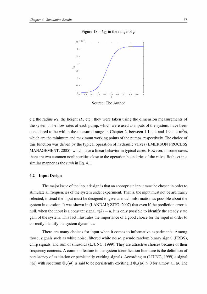
Chapter 4. Simulation Results 58
Figure 18 – k12 in the range of p
0 0.1 0.2 0.3 0.4 0.5 0.6 0.7 0.8 0.9 1p
0
0.5
1
1.5
2
2.5
3
3.5
k12
#10-3
Source: The Author
e.g the radius R1, the height Hci etc., they were taken using the dimension measurements ofthe system. The flow rates of each pump, which were used as inputs of the system, have beenconsidered to be within the measured range in Chapter 2, between 1.1e−4 and 1.9e−4 m3/s,which are the minimum and maximum working points of the pumps, respectively. The choice ofthis function was driven by the typical operation of hydraulic valves (EMERSON PROCESSMANAGEMENT, 2005), which have a linear behavior in typical cases. However, in some cases,there are two common nonlinearities close to the operation boundaries of the valve. Both act in asimilar manner as the tanh in Eq. 4.1.
4.2 Input Design
The major issue of the input design is that an appropriate input must be chosen in order tostimulate all frequencies of the system under experiment. That is, the input must not be arbitrarilyselected, instead the input must be designed to give as much information as possible about thesystem in question. It was shown in (LANDAU; ZITO, 2007) that even if the prediction error isnull, when the input is a constant signal u(k) = u, it is only possible to identify the steady stategain of the system. This fact illustrates the importance of a good choice for the input in order tocorrectly identify the system dynamics.
There are many choices for input when it comes to informative experiments. Amongthose, signals such as white noise, filtered white noise, pseudo random binary signal (PRBS),chirp signals, and sum of sinusoids (LJUNG, 1999). They are attractive choices because of theirfrequency contents. A common feature in the system identification literature is the definition ofpersistency of excitation or persistently exciting signals. According to (LJUNG, 1999) a signalu(k) with spectrum Φu(ω) is said to be persistently exciting if Φu(ω)> 0 for almost all ω . The

Chapter 4. Simulation Results 59
definition of spectrum is as follows (LJUNG, 1999):
Φu(ω) =∞
∑τ=−∞
Ru(τ)e−iτω , (4.2)
with Ru(τ) = E u(k)u(k− τ). Depending on the model structure at hand, for the case of anLTI system, a data set is said to be informative if the input is persistently exciting (LJUNG,1999). Regarding the LPV case, some caution must be taken mainly because of the extra signalinvolved, which is the scheduling variable p. One of the first papers to address this problem was(BAMIEH; GIARRÉ, 2002), where it was shown that in order to obtain an informative data setfor LPV models the two following conditions must hold.
a) There exists N distinct points pi ∈ R, i = 1, . . . ,N that are limit points of p(k).
b) The system must be excited by a persistently exciting input in every point of thescheduling variable.
A recent paper that addresses the problem of informative data in the LPV framework is(DANKERS et al., 2011). Due to the lack of transfer function representation in the LPV case, in(DANKERS et al., 2011) it was considered equality in terms of predicted output and identifia-bility of the LPV-ARX structure is studied. However, the problem of how to choose an optimalinput that delivers an informative experiment regarding practical applications is still subject forfurther research.
For the experiments made in this thesis, it was chosen a combination of PRBS type forthe input u and a sinusoidal signal for the scheduling variable p. Such a choice is adequateregarding the conditions in a) -b) . The experiments are carried out with this setting. The PRBSis defined as follows (LJUNG, 1999):
u(k) = rem(A(q)u(k),2) = rem(a1u(k−1)+ · · ·+anu(t−n),2) , (4.3)
here rem(x,2) refers to the remainder as x divided by 2 which is equivalent to a modulo-2operation. Thus, u(k) only assumes 0 and 1 values. After u is generated, it is possible to convertto any two desired levels. The vector of past inputs can only assume 2n values (LJUNG, 1999).In fact, since n consecutive zeros would further lead u to the same state, u must be periodicwith a maximum period of M = 2n−1. It can be shown that for any n, there are choices of thepolynomial A(q) that yield to a maximum period length (LJUNG, 1999). Table 4 summarizessuch choices. There is another interpretation for the PRBS design. The modulo-2 operation isequivalent to a logical xor operation. In this way, a vector of n bits can be created and the xoroperation is carried out only with some selected bits for each n, similar to the choice of thenonzero parameters ak in Eq.4.3. Both procedures lead to the same sequence for the same choiceof n. The latter procedure can be seen in (LANDAU; ZITO, 2007). Figure 19 illustrates thePRBS design using the xor procedure. The interest in the PRBS signal is due to its frequencycontents. In (LJUNG, 1999) is shown that any maximum length PRBS behaves like a periodic

Chapter 4. Simulation Results 60
Table 4 – Choice of the nonzero elements in A(q) for the PRBS design
Order n length M k for ak = 1
2 3 1,23 7 2,34 15 1,45 31 2,56 63 1,67 127 3,78 255 1,89 511 4,9
10 1023 7,1011 2047 9,11
Source: (LJUNG, 1999)
Figure 19 – PRBS design using the logic xor
a1 a2 a3 a4 a5 a6 a7 a8 a9
XOR
n bits
Source: The Author
white noise. The comparison with white noise is made here because of its properties, which is auniform contribution to the power spectrum density for all ω (TANGIRALA, 2014).
4.3 Identification Experiment in the Simulation Setting
In this section the data generator system is presented and an appropriate input is designedbased on the previous section for the identification experiment. To the best of the author’sknowledge, the problem of optimal input design for the LPV case was not directly addressedyet. Therefore, a general approach for LTI systems was chosen to be followed in this thesis. Theselected input was two PRBS signals, with one being a shifted version of the other. The procedureof the PRBS design was chosen as the one indicated in (LANDAU; ZITO, 2007). The amplitudeof the PRBS was chosen in order to maximize the entire operation region of the system, that is,the first value was chosen as the minimum flow rate of the pumps, while the second was chosenas the maximum flow rate of the pumps. Recall that the PRBS has similar properties to the whitenoise, but the latter in practice is usually not feasible. In order to correctly identify the dominantpoles of the system, a step response experiment was done for the minimum and maximum outputof the pumps. Figure 20 illustrates the step response of the two-tank systems. There are some

Chapter 4. Simulation Results 61
Figure 20 – The step response of the system
0 20 40 60 80 100 120 140Time (s)
0
0.02
0.04
0.06
0.08
0.1
0.12
heig
ht (
m)
Minimum flow rate
h1
h2
(a) Minimum flow rate step response
0 50 100 150 200 250 300 350 400Time (s)
0
0.05
0.1
0.15
0.2
0.25
0.3
0.35
0.4
heig
ht (
m)
Maximum flow rate
h1
h2
(b) Maximum flow rate step response
Source: The Author
conditions that a PRBS must satisfy in order to maximize the information about the system athand. The first condition is that the PRBS spectrum must be constant at the frequency of thedominant poles. A second condition is that in order to identify the steady state gain the maximumpulse length (when all bits of the PRBS are equal to one) must be greater than the system’s risetime (LANDAU; ZITO, 2007). Again, it is worthy to remind that there is no general approach toinput design in the LPV framework. Therefore, it will be followed the general approach for LTIsystems.
As Figure 20 indicates, there is a difference between the step responses either in the staticgain and time constant for each input. This illustrates the well-known nonlinear behavior of thesystem. However, an important feature of the system is its first order behavior. For any flow-rateused as input, there are no changes of concavity in the step response, thus characterizing a plantwith only real poles, which can be successfully approximated by a first order transfer function ina determined working point. The slowest rise time is about 100 seconds, whereas the fastest isabout 42 seconds. The latter rise time can be discarded as the slow pole plays a more importantrole in the dynamics of the system.
The first parameter that must be chosen in the experiment setup is the sampling rateof the process. Regarding the fastest time constant is equal to 59 seconds, a general guidelineis to choose the sampling time between Ts/5 and Ts/10 (TANGIRALA, 2014) with Ts beingthe dominant time constant. The sampling time was chosen as 0.5 seconds considering that inthe real system the output valves may vary with time. Depending on their outlet constant thetime constant could be fewer than 5 seconds. In order to efficiently design a PRBS signal toexcite the dominant poles of the plant it is necessary to choose a number of bits n and a PRBStime sampling (TPRBS) to excite the dominant poles of the system (LANDAU; ZITO, 2007). The

Chapter 4. Simulation Results 62
PRBS time sampling corresponds to the time in which the bits in the PRBS register are shifted.As mentioned previously, the maximum length pulse of a PRBS signal is equal to the numberof bits n. If the PRBS sampling frequency is chosen the same as the process’s sampling time,the maximum pulse will be equal to 5.5 seconds considering n equals to 11, which is far fromthe slowest rise time. Recall that the maximum pulse length is n∗TPBRS. Instead of increasingthe n value and consequently increasing the total length of the experiment, this was avoidedby changing the clock frequency of the PRBS signal with a TPRBS = 15 seconds and choosinga number of bits n = 7. Figure 21 illustrates the periodogram of the designed PRBS. In order
Figure 21 – Periodogram of the designed PRBS
10-3 10-2 10-1 100 101
Frequency (rad/s)
10-10
10-5
100
105
PR
BS
Frequency of interest
Source: The Author
to provide a meaningful simulation experiment, an additive white noise was added to the TTSoutputs, both independent from each other. Moreover, in order to quantify how much noiseis added in each output channel, it was considered the signal-to-noise ratio(SNR) defined as(TANGIRALA, 2014):
SNR =var(signal)var(noise)
(4.4)
where var(u) stands for the variance of the signal u. Usually, in the system identificationframework, signal in Eq. 4.4 refers to the noise free output(true response) of the system at hand.This measure must be viewed as the ratio between the effects of a known variable versus theuncertainties. Several scenarios with different SNRs will be analyzed in this experimental setupinvestigation. Thus the data generator system is as follows:
yi(k) = hi(k)+ ei(k), for i = 1,2, (4.5)
where the index i refers to each tank, ei is a white noise process, hi is the output of the i-th tank,yi is the noisy simulated output of the i-th tank. The height of each tank can be calculated throughEqs. 2.17a-2.17c from Chapter 2 in the continuous domain. Regarding hi(k), it can be simplyobtained by sampling the continuous version using the specified sampling rate. Thus, ei(k) canbe regarded as a specific noise due to the sampling measurements. Figure 22 illustrates the inputand the scheduling variable used in the simulated data.

Chapter 4. Simulation Results 63
Figure 22 – DE - Input and Scheduling variable
0 500 1000 1500 2000 2500 3000 3500 4000Samples
1.1
1.2
1.3
1.4
1.5
1.6
1.7
1.8
1.9
2
Flo
w r
ate
(m3/s
)
#10-4
u1
u2
(a) Input
0 500 1000 1500 2000 2500 3000 3500 4000Samples
0
0.1
0.2
0.3
0.4
0.5
0.6
0.7
0.8
0.9
1
Ope
nnes
s of
the
inte
rcon
nect
ion
valv
e (%
)
(b) Scheduling Variable
Source: The Author
Figure 23 shows the outputs produced by the inputs from Fig. 22 for different noisescenarios.
Figure 23 – DE - Outputs
0 500 1000 1500 2000 2500 3000 3500 4000Samples
0
0.05
0.1
0.15
0.2
0.25
0.3
0.35
wat
er h
eigh
t (m
)
y1
y2
(a) Noise-free
0 500 1000 1500 2000 2500 3000 3500 4000Samples
0
0.05
0.1
0.15
0.2
0.25
0.3
0.35
wat
er h
eigh
t (m
)
y1
y2
(b) Low Noise (SNR = 30dB)
0 500 1000 1500 2000 2500 3000 3500 4000Samples
-0.05
0
0.05
0.1
0.15
0.2
0.25
0.3
0.35
0.4
wat
er h
eigh
t (m
)
y1
y2
(c) Heavy Noise (SNR = 10 dB)
Source: The Author
4.4 Model Structure
The nonlinear modeling allowed some prior knowledge about the system at hand. Theyare listed as follows:
a) Since the equations that describe the system behavior (Eqs. 2.17a-2.17c) involve onlyfirst order derivatives, the model orders (na and nb) are both likely to be equal to one;
b) The nonlinearity involved in the system process is known and it depends on thesquare root of the water height in both tanks;
Chapter 4. Simulation Results 64
c) Since the derivatives depend only in terms up to the same time instant, there is nodead time in this process;
d) The stochastic effect in the plant is a nonlinear output error (NOE) type.
Regarding this prior knowledge, it was considered the polynomial orders (na, nb and nk) as equalto one. As it comes to the scheduling dependence, for the methods that need a parametrization inthe scheduling function, it was considered a third order polynomial dependence on the schedulingvariable.
The model structures considered herein for identification purposes are ARX and OE type.Both structures considered here were motivated by the fact that the system is in output errorform.
4.5 Results
In this section, it will be shown the results of the methods presented in Chapter 3 forthe simulation experiment. As mentioned in the previous section, the scheduling function waschosen to be of polynomial dependence. The models will be denoted as the model structure andits orders, e.g. a model ARX(NA, NB, NK, [NP]) represents a model with ARX structure withthe following orders in the operator q, na = NA, nb = NB, nk = NK and polynomial dependenceon the scheduling np = NP. In order to access the quality of a model, the Best Fit Score (BFS) isused, which is defined as (LJUNG, 1999):
BFS = 100%(
1− ||y− y||2||y− y||2
), (4.6)
where y refers to the average of signal y, y is the predicted (or simulated) output from themodel and y is the actual system response. This measure is related to how good the model isin explaining the measured signal. It works as a fitness function, lower values indicate that themodel failed to describe the system behavior, while a higher value shows a good fit. This way ofanalyzing the goodness of a model is widely used, including in the System Identification toolboxfor Matlab (LJUNG, 2007).
Recall that the model tries to explain the input-output behavior. In this context it wasconsidered the water height as output and the inlet flow-rate as the input of the model. In the LPVframework the scheduling variable plays an important role at explaining the system behavior indifferent working points. In this model it was considered the scheduling variable as the constantk12 of the valve between the two tanks. The difference equation that describes the IO behavior ofthe two tanks is given as:
yi(k) =−ai1(p(k))yi(k−1)+bi01(p(k))u1(k−1)+bi02(p(k))u2(k−1) for i = 1,2, (4.7)
where the index i refers to each tank. The data was generated using a PRBS signal specified inSec. 4.2. For each input a shifted version of the same PRBS was used. The data set, which has a
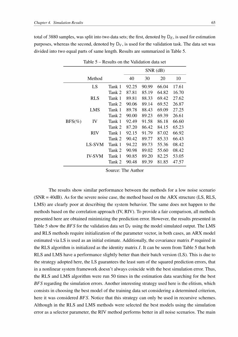
Chapter 4. Simulation Results 65
total of 3880 samples, was split into two data sets; the first, denoted by DE , is used for estimationpurposes, whereas the second, denoted by DV , is used for the validation task. The data set wasdivided into two equal parts of same length. Results are summarized in Table 5.
Table 5 – Results on the Validation data set
SNR (dB)
Method 40 30 20 10
LS Tank 1 92.25 90.99 66.04 17.61Tank 2 87.81 85.19 64.82 16.70
RLS Tank 1 89.81 88.33 69.42 27.62Tank 2 90.06 89.14 69.52 26.87
LMS Tank 1 89.78 88.43 69.09 27.25Tank 2 90.00 89.23 69.39 26.61
BFS(%) IV Tank 1 92.49 91.58 86.18 66.60Tank 2 87.20 86.42 84.15 65.23
RIV Tank 1 92.15 91.79 87.02 66.92Tank 2 90.42 89.77 85.33 66.43
LS-SVM Tank 1 94.22 89.73 55.36 08.42Tank 2 90.98 89.02 55.60 08.42
IV-SVM Tank 1 90.85 89.20 82.25 53.05Tank 2 90.48 89.39 81.85 47.57
Source: The Author
The results show similar performance between the methods for a low noise scenario(SNR = 40dB). As for the severe noise case, the method based on the ARX structure (LS, RLS,LMS) are clearly poor at describing the system behavior. The same does not happen to themethods based on the correlation approach (IV, RIV). To provide a fair comparison, all methodspresented here are obtained minimizing the prediction error. However, the results presented inTable 5 show the BFS for the validation data set DV using the model simulated output. The LMSand RLS methods require initialization of the parameter vector, in both cases, an ARX modelestimated via LS is used as an initial estimate. Additionally, the covariance matrix P required inthe RLS algorithm is initialized as the identity matrix I. It can be seem from Table 5 that bothRLS and LMS have a performance slightly better than their batch version (LS). This is due tothe strategy adopted here, the LS guarantees the least sum of the squared prediction errors, thatin a nonlinear system framework doesn’t always coincide with the best simulation error. Thus,the RLS and LMS algorithm were run 50 times in the estimation data searching for the bestBFS regarding the simulation errors. Another interesting strategy used here is the elitism, whichconsists in choosing the best model of the training data set considering a determined criterion,here it was considered BFS. Notice that this strategy can only be used in recursive schemes.Although in the RLS and LMS methods were selected the best models using the simulationerror as a selector parameter, the RIV method performs better in all noise scenarios. The main

Chapter 4. Simulation Results 66
reason for that is that the IV method performs well independently of the noise structure. A morerealistic scenario in the TTS is the 30dB SNR case. Regarding the (IV)LS-SVM case , RBFKernels were chosen (see Eq. 3.76) for the regressors and their hyper-parameters are tuned usingcross-validation. The hyper-parameters obtained are σ1 = 0.7, σ2 = 0.5,σ3 = 2.2,γ1 = 6.2∗1011
for tank 1 and σ1 = 0.5, σ2 = 0.4,σ3 = 2,γ1 = 4.5∗1011 for tank 2. This procedure was doneconsidering the noise-free version of the outputs. This is why the LS-SVM performs so badly ina heavy noise scenario compared to the other methods, the same does not happen with its IVcounterpart (IV-SVM). However, in a low noise scenario the LS-SVM outperforms all the othermethods. It should be remarked that a proper selection of the hyper-parameters may improve theresults for the SVM-based methodology.
4.6 A Single Tank in the LPV Framework
The models obtained so far have a representative system behavior regarding the mea-surements from data. In this section, a single tank model will be derived in the LPV framework.This is done here for a better understanding of the tank model in the LPV form. Here, the noiseeffects will not be considered as the main interest is the ability of an LPV model in describing anonlinear system. Recall the nonlinear model of a single tank from Sec. 2.2. Because no exoge-nous signal is present in this scheme, the scheduling variable will be considered as the waterheight, which is also the system output. In this case, the model is called quasi-LPV (q-LPV),which is motivated by the fact that the scheduling variable is an endogenous signal. The system’sinput is the inlet flow-rate, thus the system is a SISO. If needed the reader should revisit Chapter2 for the modeling part, the system scheme can be seem in Figure 3. The nonlinear dynamic wasdescribed in Eq. 2.7.
In order to describe this system in the LPV framework, it will be considered a SISO-LPVModel with polynomial dependence on the scheduling variable. Additionally, the schedulingdependence is static as the entire thesis only deals with this kind of dependence, there is noreason to do otherwise. The polynomial dependence was chosen as third order degree. Again,the BFS defined in Eq. 4.6 will be used as a measure of models’ goodness using the simulationerror. The model structure used is the following:
y(k) =−a1(p)y(k−1)+b0(p)u(k−1), (4.8)
with a1(p) = a10 + a11 p(k) + a12 p2(k) + a13 p3(k) and b0(p) = b00 + b01 p(k) + b02 p2(k) +
b03 p3(k). As there is no noise involved, it will be used the LS method to estimate an LPVmodel for the nonlinear process. Using a similar PRBS signal adopted in the previous section anLPV model was obtained using the LS method and it was achieved a BSF equivalent to 99.56%,which clearly denotes that the estimated model reproduces the nonlinear behavior. Althoughthis model responds well enough, it has eight parameters. Looking for the first-principle modelobtained in Eq. 2.7, it is clear that the scheduling variable chosen here is not directly related to

Chapter 4. Simulation Results 67
the input. Hence, the terms in the B(p,q) polynomial that depend on p are possibly not relevantfor the LPV model. This means that only the A(p,q) depends on the scheduling chosen, whichreveals an important question about the proper choice of the scheduling variable. The problem ofchoosing the scheduling variable p is not addressed in this work, but the signal p could be chosenas the nonlinearities involved in the process making the overall system linear. Now it was chosenan LPV-ARX(1, 1, 1, [4, 1]) structure, where the polynomial dependence on p in the B term waschosen as 0. For comparison reasons an LTI-ARX Model was identified as well. Table 6 showsthe BFS achieved by these models. As expected, the influence of p in the polynomial B(q, p)
Table 6 – Results of the models for a single tank
Model BFS
LPV-ARX(1,1,1, [4 4] ) 99.56%LPV-ARX(1,1,1, [4 1] ) 99.51%LTI-ARX(1,1,1) 57.23%
Source: The Author
is irrelevant. Notice that the BFS achieved by a simpler LPV-ARX model, which eliminatesthe dependence of the scheduling variable in the numerator term, is only marginally decreased.The BFS from the LTI-ARX model reveals the superiority of the LPV model in reproducing anonlinear system.
4.7 An LPV Model with 2 Scheduling Variables
Motivated by the results in the previous section it was proposed an LPV model with twoscheduling variables to identify the two-tank system. In the LPV system identification literatureonly few papers have dealt with more than one scheduling variable, more specifically with two.In (HUANG et al., 2012) an LPV system with two scheduling variables is identified using amulti-model approach. This approach is very close to the concept of the LPV system. In fewwords, it is an approach that considers a system with a response related to many LTI systemsin different working points, each LTI system has a specific weight that depends on the workingpoint. Notice that considering only one scheduling variable gives a wide amount of possibilities.In fact, many function structures can be used, e.g. affine, polynomial, irrational, etc. In the casewhere two variables are considered, the combination of them make the possibilities become evenwider. Here it is proposed an LPV model with two scheduling variables as follows:
y(k) =−na
∑i=1
(ai p1)y(k− i)+nb
∑i=0
q−nk (bi p2)u(k− i) (4.9)
where stands for a specific operation in the respective scheduling space. Notice that in thismodel there is no relationship between the scheduling variables, more precisely, each schedulingis only related either to the output dynamics or to the input dynamics. This kind of structure

Chapter 4. Simulation Results 68
is similar to the model structures used so far in this thesis. As there is no connection betweenthe scheduling of input and output, then there are no connection possibilities between the twoscheduling variables. This preserves the model’s complexity in the same way as the modelsdiscussed so far. The only difference is that there is an additional scheduling involving only theinput, whereas the other one is related to the output. To the best of the author’s knowledge, thereis no such treatment for models with two scheduling variables, and even the academic literatureassumes that there is a combination between the scheduling variables.
4.8 The TTS with 3 Scheduling Variables
In this section it was used the model structure from the previous section to describe thetwo-tank system behavior. Notice that each MISO system that describes the TTS outputs willhave only two scheduling variables, while the overall system will have dependence on threescheduling variables. The choice of the first scheduling variable is still the constant k12 betweenthe two tanks. Motivated by the results from Sec. 4.6 , the two remaining scheduling variablesare the two water heights from each tank. Recall from Eqs. 2.17a-2.17c that the schedulingvariable k12 only has relationship with the input, whereas the water height from each tank haverelationship with their respective output. It should be remarked that this model is q-LPV due tothe use of an endogenous signal (water height). It was also considered the prior knowledge ofthe model structure. Thus, it was chosen the following structure to describe the TTS behavior:
y1(k) =−a11(p2(k))y1(k−1)+b101(p1(k))u1(k−1)+b102(p1(k))u2(k−1)
y2(k) =−a21(p3(k))y2(k−1)+b201(p1(k))u1(k−1)+b202(p1(k))u2(k−1)
(4.10)
(4.11)
with p1 being the constant k12, p2, p3 the water’s height in tank 1 and 2, respectively. Exactlythe same procedure was done for the identification setting using this new model. In order tocompare the results of this new model with the results from Sec. 4.5 it was chosen the SNR of30dB to compute the estimates and analyze the BFS for both models. Table 7 summarizes theresults in the validation data. In order to perform the identification experiments, exactly the sameprocedure of Sec. 4.5 was done. Notice that in all methods the proposed model performs betterthan the model using only one scheduling variable. It should be remarked that in some methods asignificant increase of quality is obtained for the model that describes the tank 2 system. Besides,the model complexity is not increased since the additional scheduling variables are endogenousand they have been already measured as outputs. Notice that in all identification methods theTTS with three scheduling variables has a better performance in terms of BFS.
4.9 The Final Choice
In order to provide an assessment of model quality from the estimation methods adopted,it was considered a third data set DIV regarding the step response in different working points.This is naturally justified by the LPV system’s nature. This data set is completely independent

Chapter 4. Simulation Results 69
Table 7 – Results on the Validation data set with SNR = 30dB
Method TTS TTS-3S
LS Tank 1 90.99 91.97Tank 2 85.19 93.56
RLS Tank 1 88.33 91.66Tank 2 89.14 91.61
LMS Tank 1 88.43 91.63Tank 2 89.23 91.58
BFS(%) IV Tank 1 91.58 92.85Tank 2 86.42 93.94
RIV Tank 1 91.79 92.78Tank 2 89.77 90.66
LS-SVM Tank 1 89.73 92.27Tank 2 89.02 90.21
IV-SVM Tank 1 89.20 92.37Tank 2 89.39 90.20
Source: The Author
from those used so far. At this point, the analysis will be carried out graphically, instead of usingthe numerical results to assess the model’s goodness.
Recall that there are two model structures in this thesis. Basically, one that has onlyone scheduling variable, whereas the other has three scheduling variables. The former will bedenoted simply by LPV-TTS, while the latter will be denoted as LPV3S-TTS. Both have a similarstructure, which is ARX(1,1,1, [4, 4, 4]) and OE(1, 1, 1, [4, 4, 4]) for the RIV method. As in the30dB noise scenario all methods had a similar performance for the LPV3S-TSS, the estimatesfrom the IVM were chosen due to its greater BFS. While for the LPV-TSS the estimates fromthe RIV method were chosen. Additionally, an LTI system with ARX structure was identifiedusing the system identification toolbox for Matlab R©. Figure 24 and 25 illustrate the best modelsof each model structure. Table 8 shows the parameters from the models obtained through theidentification methods.
This data set is particularly interesting because it is made of many step levels in bothinputs and at the same time the scheduling variable also changes. Thus, the model is tested in awide variety of working points. Figure 26 shows the inputs and the scheduling variable used togenerate the data set DIV . It can be seem from the results that the model LPV-TTS, despite itsgood performance on the identification data set, can’t successfully describe the IO behavior ofthe system. The model fails in reproducing the appropriate gain at many working points, evenif its dynamics is well captured. The same doesn’t happen to the LPV3S-TTS model, whichmaintains the same performance in all working points. From this viewpoint, the choice of theLPV3S-TTS as the model that better describes the system behavior is clear. For comparisonpurposes, an LTI model is identified using the system identification toolbox for Matlab R©. It is

Chapter 4. Simulation Results 70
Table 8 – Parameters of the models obtained
Model Method a10 a11 a12 a13
LPV-TTS RIV Tank 1 -0.9678 0.0221 -0.0438 0.0256Tank 2 -0.9692 0.0114 0.0068 -0.0144
LPV3S-TTS IV Tank 1 -0.9678 0.3069 -2.1022 2.1437Tank 2 -1.1210 0.7045 -0.8021 0.1005
b100 b101 b102 b103
LPV-TTS RIV Tank 1 62.57 -155.33 163.39 -37.95Tank 2 -13.67 182.63 -294.94 157.96
LPV3S-TTS IV Tank 1 4.88 -114.88 208.19 -106.82Tank 2 7.14 199.67 -281.63 117.51
b200 b201 b202 b203
LPV-TTS RIV Tank 1 -12.70 163.22 -163.10 32.13Tank 2 61.59 -187.68 362.71 -218.57
LPV3S-TTS IV Tank 1 -13.45 23.62 143.40 -173.72Tank 2 73.74 -142.44 165.01 -48.33
Source: The Author
Figure 24 – Results for the LPV-TTS with the RIV method on DIV
0 100 200 300 400 500 600 700 800 900 1000Time (s)
0
0.05
0.1
0.15
0.2
0.25
0.3
0.35
heig
ht (
m)
Tank 1
trueLPV model
(a) Tank 1
0 100 200 300 400 500 600 700 800 900 1000Time (s)
0
0.05
0.1
0.15
0.2
0.25
0.3
0.35
heig
ht (
m)
Tank 2
trueLPV model
(b) Tank 2
Source: The Author
clear the improvement of the LPV framework related to all working points of the system. Table 9summarizes the results for the models obtained regarding the BFS performance on the validationdata set. A important remark must be mentioned when the scheduling variable p1 comes close tozero (the interconnected valve is virtually closed). When this happens, the TTS becomes twoindependent SISO systems as there is no coupling between the tanks. Naturally, in the regressionapproach there are terms of both inputs in the model. Ideally, the terms b20 and b10 in the modelsof Tanks 1 and 2, respectively, should be zero when p1 is zero.

Chapter 4. Simulation Results 71
Figure 25 – Results for the LPV3S-TTS with the IV method on DIV
0 100 200 300 400 500 600 700 800 900 1000Time(s)
0
0.05
0.1
0.15
0.2
0.25
0.3
0.35
heig
ht (
m)
Tank 1
trueLPV ModelLTI Model
(a) Tank 1
0 100 200 300 400 500 600 700 800 900 1000Time(s)
0
0.05
0.1
0.15
0.2
0.25
0.3
0.35
heig
ht (
m)
Tank 2
trueLPV ModelLTI Model
(b) Tank 2
Source: The Author
Figure 26 – Input and scheduling sequence of DIV
0 200 400 600 800 1000 1200Time (s)
0
0.2
0.4
0.6
0.8
1
1.2
1.4
1.6
1.8
2
flow
rat
e (m
3/s
)
#10-4
0.1
0.2
0.3
0.4
0.5
0.6
0.7
0.8
0.9
1
p(k)
Input u and scheduling sequence
u1
u2
p
Source: The Author
4.10 Summary of the Chapter
In this chapter it was shown the simulation results for the identification of a nonlineartwo tanks process. It was presented the simulation aspects of the experiment and how to obtainan appropriate choice of the input in order to excite all the modes of the system at hand. Theidentification methods described in Chapter 3 were performed in order to obtain a suitable modelfor the TTS in the LPV framework. Additionally, an LPV model was identified for one singletank process and its scheduling dependence analyzed. It was shown that the scheduling variablefor a single tank does not affect the input. This result is not surprising according to the model
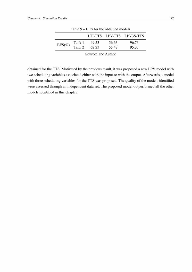
Chapter 4. Simulation Results 72
Table 9 – BFS for the obtained models
LTI-TTS LPV-TTS LPV3S-TTS
BFS(%)Tank 1 49.53 56.63 96.73Tank 2 62.23 55.48 95.32
Source: The Author
obtained for the TTS. Motivated by the previous result, it was proposed a new LPV model withtwo scheduling variables associated either with the input or with the output. Afterwards, a modelwith three scheduling variables for the TTS was proposed. The quality of the models identifiedwere assessed through an independent data set. The proposed model outperformed all the othermodels identified in this chapter.
73
5 CONCLUSION
In this chapter the overall conclusions about the subject of this thesis are pointed. Thisthesis can be outlined as follows, in chapter 2 a modeling procedure was done in order to obtain afirst-principles model based on mass conservation. Chapter 3 presents the LPV framework and themethods used for the identification of LPV models used in this thesis. In chapter 4 a simulationstudy is carried out in which is showed how an LPV model can successfully represent nonlinearsystem behavior. Besides, a new LPV model based on two scheduling variables independentlyassociated with the input and output was presented. It was shown that this method had a betterperformance in describing the TTS behavior.
The main objective of this thesis was to provide a MIMO LPV model capable of repre-senting the two-tank system. For this reason, the techniques developed in the academic literaturewere extended to the MIMO case. Throughout this thesis, the identification task was performedusing the global approach and no investigation was done with respect to appropriate choice ofbasis functions. The motivation behind that lies in the good properties of polynomial basis inapproximating functions as well as it is desired in any finite interval. Furthermore, it was used anon-parametric approach driven by the use of support vector machines. The use of the LS-SVMstrategy provides the identification of the underlying dependencies without defining an appropri-ate function basis a priori. However, as presented in the simulation study, the LS-SVM had asimilar result compared to the regression approach. In order to cope with a more general noisescenario, an instrumental variable approach adapted to the LPV-SVM case from the nonlineargeneral case. All the methods presented in this thesis had a similar performance, with the IVbased methods providing slightly better results. Based on prior knowledge of the system at handa new LPV model was developed in order to provide meaningful scheduling dependence in theparameters. This new model has had much better performance in describing the IO behavior in anew independently generated data set.
A secondary goal was to provide a first-principles model for the two-tank system. Thiswas done using the mass conservation law. This kind of modeling in tank systems was widelyused in academic research. However, to the best of the author’s knowledge, no procedure relatingdifferent shapes on the geometry of the tank was addressed. The procedure presented in thisthesis follows directly from differential calculus and it is directly related to the volume and itsderivatives. Complex shapes may turn the problem of building a first-principles model infeasiblewithin this procedure.
This work has generated the following publication:
a) MELO, F. E. M. ; NOGUEIRA, F. G. ; BARRA JR., W. ; DA COSTA, CARLOST. ; LANA, J. J. ; RIOS, C. S. ; BRAGA, A. P. S. . Least Squares and LS-SVM LPV
Chapter 5. Conclusion 74
Identification Methods with Application on a Generating Units. In: IEEE ArgenconProceeedings, Buenos Aires, 2016.
Recommendations
There were many open problems in this thesis. Here it is showed some recommendationsfor future research.
a) In this thesis is assumed that the scheduling variable is a noise-free signal. This isa non-realistic scenario in practice due to the measuring sensors. Thus, one can notaccess the noise free version of the scheduling variable. Only few works in academicresearch have coped with this issue. Additionally, some of them have selected aproper basis to analyze this problem. An interesting area of research would be toanalyze the LPV identification with the eyes of an errors-in-variables approach inorder to deal with the noise in the scheduling variables.
b) The instrumental variable method provides good estimates in the presence of colorednoise. However, only few works dealt with a scheduling dependent noise structure.Investigation of p-dependent moments (standard deviation that depends on p) in thenoise structure would be interesting for the local approach.
c) The choice of adequate instruments in the IV method is basically driven by the linearcase. Some works had shown that this approach can be successfully extended to theLPV case for a specific scheduling function dependence. The choice of the instru-ments in the nonlinear case is still an open problem. With respect to the LPV case,to the best of the author’s knowledge, a general approach regarding the schedulingstructure was not addressed yet.
d) In the recent kernel methods (LS-SVM), the choice of an adequate kernel hasparamount importance on the performance of the method. Thus, the quest for kernelsthat provide better estimates is now an active research area. A comparison amongkernel structures would be beneficial to the LPV system identification area.
e) With the development of the kernel methods, the identification task using the Bayesianperspective is currently a research topic in many works. Naturally, this is a gooddirection for future works.
f) Few works had dealt with the problem of input design in the LPV framework.Hence, a very practical task is how to get informative data sets for LPV systems.Specially, regarding the two approaches (local and global) for data gathering in theLPV framework.
g) The new LPV model presented here was inspired by an observation of the processvariables involved in the nonlinear tank model. An analysis in the point of view of

Chapter 5. Conclusion 75
system theory would benefit the application of this model. Moreover, it could beverified for what other systems this model can be successfully applied.

76
BIBLIOGRAPHY
ABBAS, H. S.; TÓTH, R.; WERNER, H. State-Space realization of LPV Input-Output models:practical methods for the user. In: American Control Conference (ACC), 2010. [S.l.: s.n.], 2010.p. 3883–3888. ISBN 978-1-4244-7426-4. ISSN 0743-1619. Cited in page 18.
ABBASI, F. et al. A support vector machine-based method for LPV-ARX identification withnoisy scheduling parameters. In: 2014 European Control Conference, ECC 2014. [S.l.: s.n.],2014. p. 370–375. ISBN 9783952426913. Cited 3 times in pages 19, 37, and 54.
ABBASI, F. et al. A Bayesian approach for model identification of LPV systems with uncertainscheduling variables. In: 2015 54th IEEE Conference on Decision and Control (CDC). [S.l.]:IEEE, 2015. p. 789–794. ISBN 978-1-4799-7886-1. Cited in page 19.
ÅSTRÖM, K. J.; HÄGGLUND, T. Pid Controllers. [S.l.]: International Society for Measurementand Control, 1995. (Setting the standard for automation). ISBN 978-15-561-7516-9. Cited inpage 13.
ÅSTRÖM, K. J.; WITTENMARK, B. Adaptive control. 2. ed. [S.l.]: Dover Publications, 1994.ISBN 978-04-864-6278-3. Cited 2 times in pages 13 and 33.
BAMIEH, B.; GIARRÉ, L. Identification for a general class of LPV models. In: Proceedings ofthe 11th IFAC System Identification. [S.l.: s.n.], 1999. p. 1505–1510. Cited in page 17.
BAMIEH, B.; GIARRÉ, L. Identification of linear parameter varying models. In: Proceedings ofthe Conference on Decision and Control. [S.l.: s.n.], 1999. p. 1505–1510. ISBN 0780352505.Cited in page 17.
BAMIEH, B.; GIARRÉ, L. Identification of linear parameter varying models. InternationalJournal of Robust and Nonlinear Control, v. 12, n. 9, p. 841–853, 2002. ISSN 10498923. Cited6 times in pages 17, 37, 38, 41, 42, and 59.
BUTCHER, M.; KARIMI, A.; LONGCHAMP, R. On the Consistency of Certain IdentificationMethods for Linear Parameter Varying Systems. In: Proceedings of the 17th IFAC worldcongress. [S.l.: s.n.], 2008. p. 4018–4023. Cited 4 times in pages 18, 37, 38, and 43.
CHAPRA, S.; CANALE, R. Numerical Methods for Engineers. [S.l.]: McGraw-Hill, 2006.(McGraw-Hill higher education). ISBN 978-0-071-2429-9. Cited in page 57.
COX, P. B.; TÓTH, R. LPV State-space model identification in the Bayesian setting: A 3-stepprocedure. In: 2016 American Control Conference (ACC). [S.l.]: IEEE, 2016. p. 4604–4610.ISBN 978-1-4673-8682-1. Cited in page 20.
COX, P. B.; TÓTH, R.; PETRECZKY, M. Estimation of lpv-ss models with static dependencyusing correlation analysis. IFAC-PapersOnLine, Elsevier B.V., v. 48, n. 26, p. 91–96, 2015. ISSN24058963. Cited in page 19.
DANKERS, A. G. et al. Informative data and identifiability in LPV-ARX prediction-erroridentification. In: Proceedings of the IEEE Conference on Decision and Control. [S.l.: s.n.],2011. p. 799–804. ISBN 9781612848006. ISSN 01912216. Cited 2 times in pages 37 and 59.

Bibliography 77
DARWISH, M. et al. Bayesian Identification of LPV Box-Jenkins Models. In: Proceedings ofthe 54th IEEE Conference on Decision and Control (CDC), Osaka, Japan. [S.l.: s.n.], 2015.ISBN 9781479978854. ISSN 07431546. Cited in page 20.
EMERSON PROCESS MANAGEMENT. Control Valve Handbook. 4th. ed. [S.l.: s.n.], 2005.Cited in page 58.
FELICI, F.; VAN WINGERDEN, J.; VERHAEGEN, M. Subspace identification of MIMO LPVsystems using a periodic scheduling sequence. Automatica, v. 43, n. 10, p. 1684–1697, 2007.ISSN 00051098. Cited in page 18.
GARCIA, C. Modelagem e Simulação. 10. ed. [S.l.]: edusp, 2013. ISBN 978-85-314-0904-2.Cited 2 times in pages 24 and 27.
GEBRAAD, P. M. et al. LPV subspace identification using a novel nuclear norm regularizationmethod. In: American Control Conference (ACC), 2011. [S.l.: s.n.], 2011. p. 165–170. ISBN9781457700811. Cited in page 19.
GOLABI, A. et al. A Bayesian approach for estimation of linear-regression LPV models. In:Proceedings of the IEEE Conference on Decision and Control. [S.l.: s.n.], 2014. v. 2015-Febru,n. February, p. 2555–2560. ISBN 9781467360906. ISSN 07431546. Cited in page 19.
GOLABI, A. et al. A Bayesian Approach for LPV Model Identification and Its Application toComplex Processes. IEEE Transactions on Control Systems Technology, p. 1–8, 2017. ISSN1063-6536. Cited in page 20.
GUNES, B.; VAN WINGERDEN, J.-W.; VERHAEGEN, M. Predictor-Based Tensor Regression(PBTR) for LPV subspace identification. Automatica, Elsevier Ltd, v. 79, p. 235–243, may 2017.ISSN 00051098. Cited in page 20.
HALLIDAY, D.; RESNICK, R.; WALKER, J. Fundamentals of Physics Extended. 10. ed. [S.l.]:Wiley, 2013. ISBN 978-11-182-3072-5. Cited 2 times in pages 24 and 30.
HEUBERGER, P. S. C.; VAN DEN HOF, P. M. J.; WAHLBERG, B. Modelling andIdentification with Rational Orthogonal Basis Functions. [S.l.]: Springer London, 2005. ISBN978-18-462-8178-5. Cited in page 17.
HUANG, J. et al. Some study on the identification of multi-model lpv models with twoscheduling variables. IFAC Proceedings Volumes, IFAC, v. 45, n. 16, p. 1269–1274, jul 2012.ISSN 14746670. Cited in page 67.
KHALATE, A. A. et al. Optimal experimental design for LPV identification using a localapproach. In: Proc. of the 15th IFAC Symposium on System Identification. [S.l.: s.n.], 2009. p.162–167. ISBN 9783902661470. Cited in page 18.
LANDAU, I. D.; ZITO, G. Digital Control Systems: Design, Identification and Implementation.[S.l.]: Springer London, 2007. (Communications and Control Engineering). ISBN978-1-84628-056-6. Cited 4 times in pages 58, 59, 60, and 61.
LAURAIN, V. et al. Identification of LPV Output-Error and Box-Jenkins Models via OptimalRefined Instrumental Variable Methods. In: American Control Conference. [S.l.: s.n.], 2010.p. 0–5. ISBN 9781424474257. Cited 5 times in pages 19, 37, 41, 44, and 48.

Bibliography 78
LAURAIN, V. et al. Refined instrumental variable methods for LPV box-jenkins models.Automatica, Elsevier Ltd, v. 9781430237, n. 6, p. 27–47, 2010. ISSN 00051098. Cited 9 timesin pages 19, 37, 38, 41, 44, 45, 46, 47, and 48.
LAURAIN, V. et al. Direct identification of continous-time lpv models. In: American ControlConference. [S.l.: s.n.], 2011. Cited in page 19.
LAURAIN, V. et al. Direct identification of continuous time lpv input/output models. IETControl Theory and Applications, v. 5, n. April 2010, p. 878–888, 2011. ISSN 1751-8644. Citedin page 19.
LAURAIN, V. et al. Direct identification of continuous-time LPV input/output models. IETControl Theory and Applications, v. 5, n. April 2010, p. 878–888, 2011. ISSN 1751-8644. Citedin page 37.
LAURAIN, V. et al. An instrumental least squares support vector machine for nonlinear systemidentification. Automatica, Elsevier Ltd, v. 54, n. October, p. 340–347, 2015. ISSN 00051098.Cited in page 54.
LAURAIN, V. et al. Nonparametric identification of LPV models under general noise conditions:An LS-SVM based approach. IFAC Proceedings Volumes (IFAC-PapersOnline), v. 16, n. PART1, p. 1761–1766, 2012. ISSN 14746670. Cited 3 times in pages 19, 37, and 54.
LAURAIN, V.; ZHENG, W. X.; TÓTH, R. Introducing instrumental variables in the LS-SVMbased identification framework. In: Proceedings of the IEEE Conference on Decision andControl. [S.l.: s.n.], 2011. p. 3198–3203. ISBN 9781612848006. ISSN 01912216. Cited in page54.
LEE, L. H.; POOLLA, K. Identification of linear parameter-varying systems via LFTs. In:Proceedings of 35th IEEE Conference on Decision and Control. [S.l.: s.n.], 1996. v. 2, n.December, p. 1545–1550. ISBN 0-7803-3590-2. ISSN 0191-2216. Cited in page 17.
LEE, L. H.; POOLLA, K. Identification of linear parameter-varying systems using nonlinearprogramming. Journal of Dynamic Systems Measurement and Control, v. 121, n. 1, p. 71–78,1999. Cited in page 17.
LIU, Q. et al. Non-parametric identification of linear parameter-varying spatially-interconnectedsystems using an LS-SVM approach. In: 2016 American Control Conference (ACC). [S.l.]:IEEE, 2016. p. 4592–4597. ISBN 978-1-4673-8682-1. Cited in page 20.
LJUNG, L. System Identification: Theory for the User. 2nd edition. ed. [S.l.]: Prentice Hall,1999. ISBN 978-01-365-6695-3. Cited 15 times in pages 14, 15, 16, 35, 36, 38, 39, 41, 43, 44,56, 58, 59, 60, and 64.
LJUNG, L. System Identification Toolbox for use with Matlab, Version 7. 7th. ed. [S.l.], 2007.Cited in page 64.
LOPES DOS SANTOS, P. et al. Identification of LPV state space systems by a separable leastsquares approach. In: Proceedings of the IEEE Conference on Decision and Control. [S.l.: s.n.],2013. ISBN 9781467357173. ISSN 01912216. Cited 2 times in pages 19 and 37.
LOPES DOS SANTOS, P. et al. LPV system identification using a separable least squaressupport vector machines approach. In: 53rd IEEE Conference on Decision and Control. [S.l.]:IEEE, 2014. p. 2548–2554. ISBN 978-1-4673-6090-6. ISSN 07431546. Cited in page 19.

Bibliography 79
LOPES DOS SANTOS, P. et al. Identification of lpv systems with non-white noise schedulingsequences. IFAC Proceedings Volumes, v. 45, n. 16, p. 1755–1760, jul 2012. ISSN 14746670.Cited in page 19.
LOPES DOS SANTOS, P.; RAMOS, J.; MARTINS DE CARVALHO, J. Identification of LinearParameter Varying Systems Using an Iterative Deterministic-Stochastic Subspace Approach. In:Proceedings of the European Control Conference 2005. [S.l.: s.n.], 2007. p. 7120–7126. ISBN9783952417386. Cited 2 times in pages 18 and 37.
LOPES DOS SANTOS, P.; RAMOS, J. A.; MARTINS DE CARVALHO, J. L. Identificationof bilinear systems with white noise inputs: An iterative deterministic-stochastic subspaceapproach. IEEE Transactions on Control Systems Technology, v. 17, n. 5, p. 1145–1153, Sept2009. ISSN 1063-6536. Cited in page 19.
MAZZARO, M. C.; MOVSICHOFF, E. A.; SÁNCHEZ-PEÑA, R. S. Robust identification oflinear parameter varying systems. In: Proc. of the American Control Conference. [S.l.: s.n.],1999. v. 4, n. June, p. 2282–2284. Cited in page 17.
MOHAMMADPOUR, J.; SCHERER, C. W. Control of Linear Parameter Varying Systemswith Applications. [S.l.]: Springer New York, 2012. (SpringerLink : Bücher). ISBN978-14-614-1833-7. Cited 3 times in pages 36, 37, and 41.
NEMANI, M.; RAVIKANTH, R.; BAMIEH, B. Identification of linear parametrically varyingsystems. In: Proceedings of 1995 34th IEEE Conference on Decision and Control. [S.l.: s.n.],1995. v. 3, n. 217, p. 2990–2995. ISBN 0-7803-2685-7. ISSN 0191-2216. Cited in page 17.
NOGUEIRA, F. G. Investigação experimental de estratégias de identificação e controle LPVaplicadas ao amotercimento de oscilações eletromecânicas em sistemas elétricos de potência.PhD. Thesis — Federal University of Pará, Belem, Pará, 2012. Cited in page 36.
OPPENHEIM, A. V.; WILLSKY, A. S.; HAMID, S. Signals and Systems. 2. ed. [S.l.]: PrenticeHall, 1996. ISBN 978-01-381-4757-0. Cited 2 times in pages 34 and 35.
PETRECZKY, M.; TÓTH, R.; MERCERE, G. Realization Theory for LPV State-SpaceRepresentations with Affine Dependence. IEEE Transactions on Automatic Control, v. 9286,n. c, p. 1–1, 2016. ISSN 0018-9286. Cited in page 20.
PIGA, D. et al. LPV system identification under noise corrupted scheduling and output signalobservations. Automatica, Elsevier Ltd, v. 53, p. 329–338, 2015. ISSN 00051098. Cited 2 timesin pages 20 and 37.
PIGA, D.; TÓTH, R. Lpv model order selection in an ls-svm setting. In: Proceedings of the IEEEConference on Decision and Control. [S.l.: s.n.], 2013. p. 4128–4133. ISBN 9781467357173.ISSN 01912216. Cited in page 19.
PREVIDI, F.; LOVERA, M. Identification of a class of linear models with nonlinearlyvarying parameters. In: Proc. of the European Control Conference. [S.l.: s.n.], 1999. ISBN9783952417355. Cited in page 17.
PROIMADIS, I.; BIJL, H.; VAN WINGERDEN, J. A kernel based approach for LPV subspaceidentification. IFAC-PapersOnLine, Elsevier B.V., v. 48, n. 26, p. 97–102, 2015. ISSN 24058963.Cited in page 20.
Bibliography 80
RIZVI, S. Z. et al. A Kernel-based Approach to MIMO LPV State-space Identification andApplication to a Nonlinear Process System. IFAC-PapersOnLine, Elsevier B.V., v. 48, n. 26, p.85–90, 2015. ISSN 24058963. Cited 2 times in pages 20 and 54.
RIZVI, S. Z. et al. An IV-SVM-based approach for identification of state-space LPV modelsunder generic noise conditions. In: 2015 54th IEEE Conference on Decision and Control (CDC).[S.l.]: IEEE, 2015. p. 7380–7385. ISBN 978-1-4799-7886-1. Cited 2 times in pages 20 and 54.
ROMANO, R. A. et al. Machine learning barycenter approach to identifying LPV state-spacemodels. In: 2016 American Control Conference (ACC). [S.l.]: IEEE, 2016. p. 6351–6356. Citedin page 20.
SCHÖLKOPF, B.; SMOLA, A. Learning with Kernels: Support Vector Machines, Regularization,Optimization, and Beyond. [S.l.]: MIT Press, 2002. (Adaptive computation and machinelearning). ISBN 978-02-621-9475-4. Cited 3 times in pages 48, 49, and 53.
SHAMMA, J. Analysis and design of gain scheduled control systems. PhD. Thesis —Massachusetts Institute of Technology, Cambridge, United States, 1988. Cited in page 33.
SÖDERSTRÖM, T.; STOICA, P. Instrumental variable methods for system identification. [S.l.]:Springer, 1983. (Lecture notes in control and information sciences). ISBN 978-35-401-2814-4.Cited 4 times in pages 43, 44, 47, and 56.
SUYKENS, J.; VAN GESTEL, T.; DE BRABANTER, J. Least Squares Support VectorMachines. [S.l.]: World Scientific, 2002. ISBN 978-98-123-8151-4. Cited 4 times in pages 48,49, 50, and 51.
SUYKENS, J.; VANDEWALLE, J. Least squares support vector machine classifiers. NeuralProcessing Letters, v. 9, n. 3, p. 293–300, 1999. ISSN 1573-773X. Cited 2 times in pages 49and 51.
TANGIRALA, A. Principles of System Identification: Theory and Practice. [S.l.]: Taylor &Francis, 2014. (Chapman & Hall/CRC Biostatistics Series). ISBN 978-14-398-9599-3. Cited 3times in pages 60, 61, and 62.
TÓTH, R. Modeling and Identification of Linear Parameter-Varying Systems. 1. ed. [S.l.]:Springer-Verlag Berlin Heidelberg, 2010. (Lecture Notes in Control and Information Sciences403). ISBN 978-36-421-3811-9. Cited 6 times in pages 13, 33, 34, 36, 37, and 38.
TÓTH, R. et al. Discrete time LPV I/O and state space representations, differences of behaviorand pitfalls of interpolation. In: Proc. of the European Control Conference. [S.l.: s.n.], 2007. v. 0,n. 4, p. 5418–5425. ISBN 9789608902855. Cited in page 18.
TÓTH, R. et al. Crucial Aspects of Zero-Order Hold LPV State-Space System Discretization. In:Proceedings of the 17th IFAC World Congress. [S.l.: s.n.], 2008. p. 4952–4957. Cited in page18.
TÓTH, R.; HEUBERGER, P. S. C.; VAN DEN HOF, P. M. J. OPTIMAL POLE SELECTIONFOR LPV SYSTEM IDENTIFICATION WITH OBFs, A CLUSTERING APPROACH. IFACProceedings Volumes, v. 39, n. 1, p. 356–361, 2006. ISSN 14746670. Cited in page 18.
Bibliography 81
TÓTH, R.; HEUBERGER, P. S. C.; VAN DEN HOF, P. M. J. Orthonormal basis selectionfor LPV system identification, the Fuzzy-Kolmogorov c-Max approach. In: Proceedings ofthe 45th IEEE Conference on Decision and Control. [S.l.: s.n.], 2006. p. 2529–2534. ISBN1-4244-0171-2. ISSN 01912216. Cited in page 18.
TÓTH, R.; HEUBERGER, P. S. C.; VAN DEN HOF, P. M. J. LPV system identification withglobally fixed orthonormal basis functions. In: Proceedings of the IEEE Conference on Decisionand Control. [S.l.: s.n.], 2007. p. 3646–3653. ISBN 1424414989. ISSN 01912216. Cited inpage 18.
TÓTH, R.; HEUBERGER, P. S. C.; VAN DEN HOF, P. M. J. Flexible model structures for lpvidentification with static scheduling dependency. In: 2008 47th IEEE Conference on Decisionand Control. [S.l.: s.n.], 2008. p. 4522–4527. ISSN 0191-2216. Cited in page 18.
TÓTH, R.; HEUBERGER, P. S. C.; VAN DEN HOF, P. M. J. A Prediction-Error IdentificationFramework for Linear Parameter-Varying Systems. In: Proc. of the 19th InternationalSymposium on Mathematical Theory of Networks and Systems. [S.l.: s.n.], 2010. p. 1351–1352.ISBN 9789633113707. Cited in page 19.
TÓTH, R.; HJALMARSSON, H.; ROJAS, C. R. Order and structural dependence selection ofLPV-ARX models revisited. In: Proceedings of the IEEE Conference on Decision and Control.[S.l.: s.n.], 2012. p. 6271–6276. ISBN 978-1-4673-2066-5. ISSN 01912216. Cited in page 19.
TÓTH, R. et al. On the closed loop identification of LPV models using instrumental variables. In:Proc. of the 18th IFAC World Congress. [S.l.: s.n.], 2011. p. 7773–7778. ISBN 9783902661937.ISSN 14746670. Cited in page 19.
TÓTH, R. et al. Instrumental variable scheme for closed-loop lpv model identification.Automatica, Elsevier Ltd, v. 48, n. 9, p. 2314–2320, 2012. ISSN 00051098. Cited in page 19.
TÓTH, R. et al. Model Structure Learning : A Support Vector Machine Approach for LPVLinear-Regression Models. In: Conference on Decision and Control and European ControlConference. [S.l.: s.n.], 2011. p. 3192–3197. ISBN 9781612848013. Cited 6 times in pages 19,37, 48, 49, 52, and 54.
TÓTH, R. et al. A behavioral approach to lpv systems. In: 2009 European Control Conference(ECC). [S.l.: s.n.], 2009. p. 2015–2020. Cited in page 18.
TÓTH, R. et al. The behavioral approach to linear parameter-varying systems. IEEETransactions on Automatic Control, v. 56, n. 11, p. 2499–2514, Nov 2011. ISSN 0018-9286.Cited in page 18.
TURK, D.; PIPELEERS, G.; SWEVERS, J. A Combined Global and Local IdentificationApproach for LPV Systems. IFAC-PapersOnLine, Elsevier B.V., v. 48, n. 28, p. 184–189, 2015.ISSN 24058963. Cited in page 20.
UMANAND, L. Power Electronics: Essentials & Applications. [S.l.]: Wiley India, 2009. ISBN978-81-265-1945-3. Cited in page 29.
VAN OVERSCHEE, P.; DE MOOR, B. L. Subspace Identification for Linear Systems: Theory —Implementation — Applications. [S.l.]: Springer US, 1996. ISBN 978-14-613-0465-4. Cited inpage 16.

Bibliography 82
VAN WINGERDEN, J.-W.; VERHAEGEN, M. Subspace identification of Bilinear and LPVsystems for open- and closed-loop data. Automatica, Elsevier Ltd, v. 45, n. 2, p. 372–381, 2009.ISSN 00051098. Cited 2 times in pages 19 and 34.
VAPNIK, V. The Nature of Statistical Learning Theory. [S.l.]: Springer New York, 1999.(Information Science and Statistics). ISBN 978-03-879-8780-4. Cited 2 times in pages 48and 49.
VERDULT, V.; VERHAEGEN, M. Identification of Multivariable Lpv State Space Systems ByLocal Gradient Search. In: European Control Conference. [S.l.: s.n.], 2001. p. 3675–3680. ISBN9783952417362. Cited in page 17.
VERDULT, V.; VERHAEGEN, M. Subspace identification of multivariable linear parameter-varying systems. Automatica, v. 38, n. 5, p. 805–814, 2002. ISSN 00051098. Cited in page17.
VERDULT, V.; VERHAEGEN, M. Kernel methods for subspace identification of multivariableLPV and bilinear systems. Automatica, v. 41, n. 9, p. 1557–1565, 2005. ISSN 00051098. Citedin page 17.
WILLEMS, J. C. Paradigms and puzzles in the theory of dynamical systems. IEEE Transactionson Automatic Control, v. 36, n. 3, p. 259–294, Mar 1991. ISSN 0018-9286. Cited in page 18.
YOUNG, P. Recursive estimation and time-series analysis: an introduction. [S.l.]: Springer-Verlag, 1984. (Communications and control engineering series). ISBN 978-35-401-3677-4.Cited 3 times in pages 44, 47, and 48.
YOUNG, P.; JAKEMAN, A. Refined instrumental variable methods of recursive time-seriesanalysis part i. single input, single output systems. International Journal of Control, v. 29, n. 1,p. 1–30, 1979. Cited in page 44.
ZWILLINGER, D. CRC Standard Mathematical Tables and Formulae. 31. ed. [S.l.]: CRC Press,2003. ISBN 1-58488-291-3. Cited in page 25.