Linear Parameter Varying and Time-Varying Model Predictive...

02 -(C)2018A.Bemporad-“ModelPredictiveControl”course 1

Linear Parameter Varying and Time-Varying Model Predictive Control

Alberto Bemporad - “Model Predictive Control” course - Academic year 2017/18

minU

N�1X

k=0kWy(yk � r(t))k2 + kWu(uk � uref(t))k2

(xk+1 = A(p(t))xk +Bu(p(t))uk +Bv(p(t))vk

yk = C(p(t))xk +Dv(p(t))vk

(umin uk umaxymin yk ymax

minz

1

2z0H(p(t))z + ✓

0(t)F (p(t))0z

s.t. G(p(t))z W (p(t)) + S(p(t))✓(t)

02 -(C)2018A.Bemporad-“ModelPredictiveControl”course

Linear Parameter-Varying (LPV) MPC

2

quadraticperformanceindex

constraints

LTIpredictionmodel

QP

• LPVmodelscanbeobtainedfromlinearizationofnonlinearmodelsorfromblack-boxLPVsystemidentification

AllQPmatricesareconstructedonline

Model depends on time t but does not change in prediction

minU

N�1X

k=0kWy(yk � r(t))k2 + kWu(uk � uref(t))k2

(xk+1 = Ak(p(t))xk +Buk(p(t))uk +Bvk(p(t))vk

yk = Ck(p(t))xk +Dvk(p(t))vk


Linear Time-Varying (LTV) MPC

3

quadraticperformanceindex

constraints

LTVpredictionmodel

• LTVmodelscanbeobtainedfromlinearizingNLmodelsaroundtime-varyingreferencetrajectories(e.g.:previousoptimaltrajectory)

LTV-MPCstillleadstoaconvexQP

Model depends on time t and prediction step k

QP

(umin uk umaxymin yk ymax

minz

1

2z0H(p(t))z + ✓

0(t)F (p(t))0z

s.t. G(p(t))z W (p(t)) + S(p(t))✓(t)

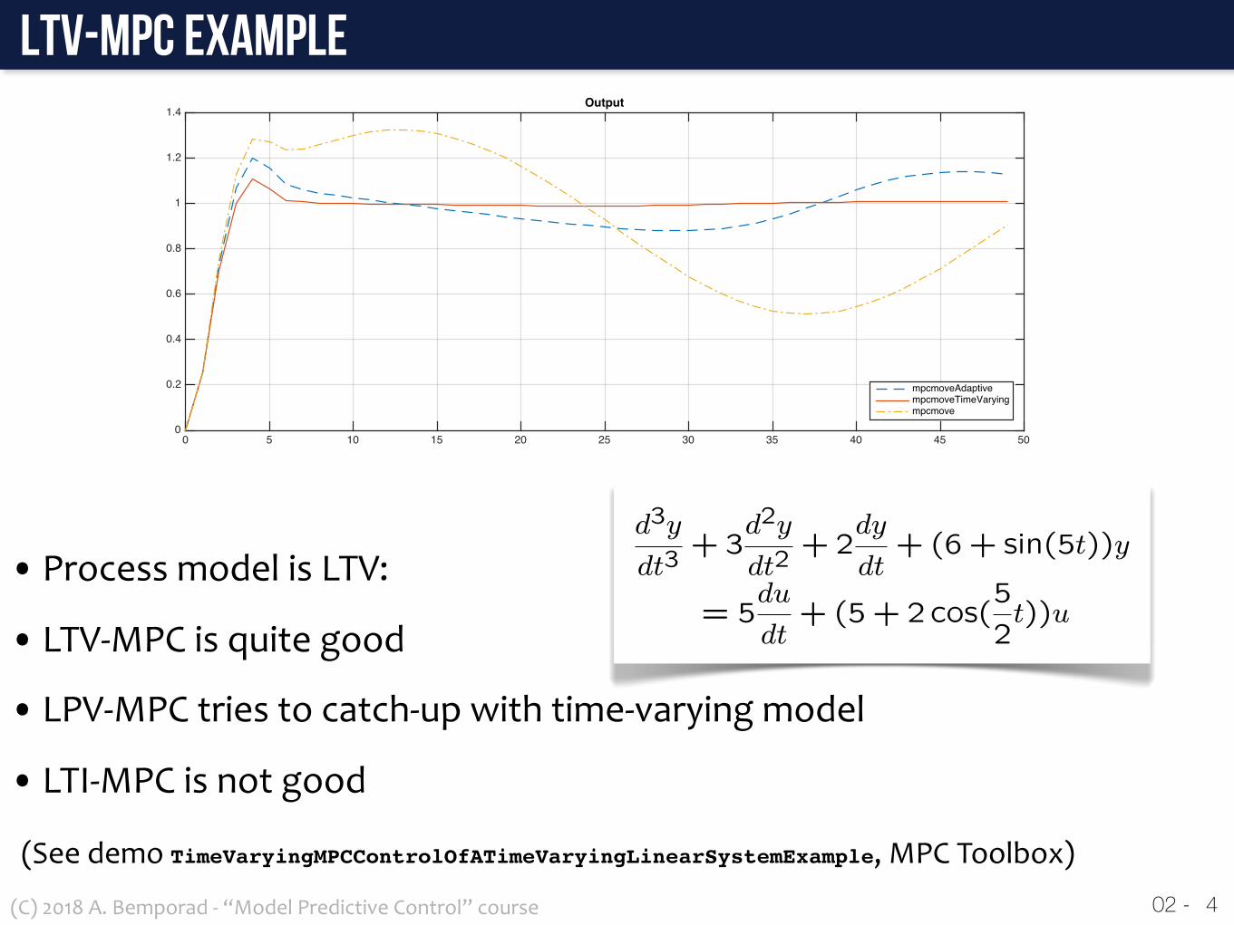
d3y

dt3+ 3

d2y

dt2+ 2

dy

dt+ (6+ sin(5t))y

= 5du

dt+ (5+ 2cos(

5

2t))u


LTV-MPC example

4

0 5 10 15 20 25 30 35 40 45 500

0.2

0.4

0.6

0.8

1

1.2

1.4Output

mpcmoveAdaptivempcmoveTimeVaryingmpcmove

0 5 10 15 20 25 30 35 40 45 50-0.5

0

0.5

1

1.5

2

2.5

3Input

• ProcessmodelisLTV:

• LTV-MPCisquitegood

• LPV-MPCtriestocatch-upwithtime-varyingmodel

• LTI-MPCisnotgood

(SeedemoTimeVaryingMPCControlOfATimeVaryingLinearSystemExample,MPCToolbox)


LTV-MPC example•DefineLTVmodel

5

Models = tf; ct = 1;for t = 0:0.1:10 Models(:,:,ct) = tf([5 5+2*cos(2.5*t)],[1 3 2 6+sin(5*t)]); ct = ct + 1;end

Ts = 0.1; % sampling timeModels = ss(c2d(Models,Ts));

•DesignMPCcontroller

sys = ss(c2d(tf([5 5],[1 3 2 6]),Ts)); % average model timep = 3; % prediction horizonm = 3; % control horizonmpcobj = mpc(sys,Ts,p,m);

mpcobj.MV = struct('Min',-2,'Max',2); % input constraintsmpcobj.Weights = struct('MV',0,'MVRate',0.01,'Output',1);


LTV-MPC example• SimulateLTVsystemwithLTIMPCcontroller

6

for ct = 1:(Tstop/Ts+1) real_plant = Models(:,:,ct); % Get the current plant y = real_plant.C*x; u = mpcmove(mpcobj,xmpc,y,1); % Apply LTI MPC x = real_plant.A*x + real_plant.B*u;end

• SimulateLTVsystemwithLPVMPCcontroller

for ct = 1:(Tstop/Ts+1) real_plant = Models(:,:,ct); % Get the current plant y = real_plant.C*x; u = mpcmoveAdaptive(mpcobj,xmpc,real_plant,nominal,y,1); x = real_plant.A*x + real_plant.B*u;end

t

uy

Time-Varying Plant

AdaptiveMPC mv

model

mo

ref

Adaptive MPC Controller

t

A

B

C

D

U

Y

X

DX

Time Varying Predictive Model

Clock

usim

To Workspace

ysim

To Workspace1

Zero-OrderHold

1

Reference


LTV-MPC example• SimulateLTVsystemwithLTVMPCcontroller

7

for ct = 1:(Tstop/Ts+1) real_plant = Models(:,:,ct); % Get the current plant y = real_plant.C*x; u = mpcmoveAdaptive(mpcobj,xmpc,Models(:,:,ct:ct+p),... Nominals,y,1); x = real_plant.A*x + real_plant.B*u;end

• SimulateinSimulink

mpc_timevarying.mdl


LTV-MPC example

8

• Simulinkblock

mpc_timevarying.mdl

need to provide 3D array of future models

• Assumemodelisnonlinearandcontinuous-time dx

dt= f(x(t), u(t))

xk+1 =

I + Ts

@f

@x

��x(t),u(t)

!xk +

Ts

@f

@u

��x(t),u(t)

!uk + fk


Linearization and TIme-Discretization

9

discrete-time LPV model

A(t) B(t)

f(t) model matrices depend on current time t

• Conversiontodiscrete-timelinearpredictionmodel

• Linearizearoundanominalstatex(t)andinputu(t),suchas:

- anequilibrium- areferencetrajectory- themostupdatedvalue

dx

dt(t+ ⌧) '

@f

@x

��x(t),u(t)

(x(t+ ⌧)� x(t))

+@f

@u

��x(t),u(t)

(u(t+ ⌧)� u(t)) + f(x(t), u(t))

dCA

dt=

F

V(CAf � CA)� CAk0e

��ERT

dT

dt=

F

V(Tf � T ) +

UA

�CpV(Tj � T )� �H

�CpCAk0e

��ERT

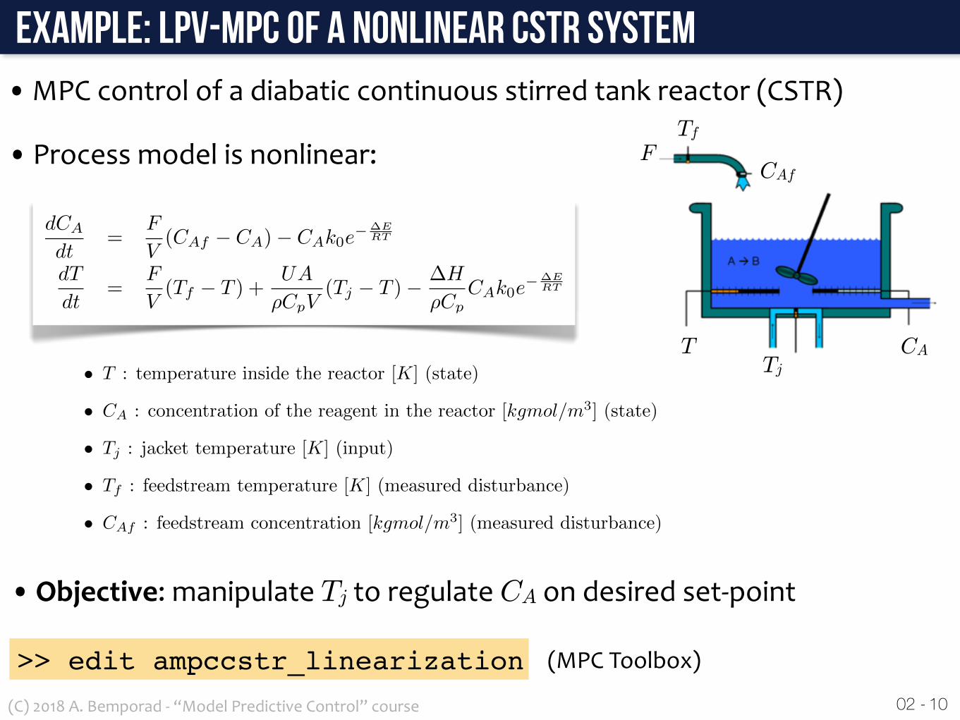
• T : temperature inside the reactor [K] (state)

• CA : concentration of the reagent in the reactor [kgmol/m3] (state)

• Tj : jacket temperature [K] (input)

• Tf : feedstream temperature [K] (measured disturbance)

• CAf : feedstream concentration [kgmol/m3] (measured disturbance)


Example: LPV-MPC of a nonlinear CSTR system•MPCcontrolofadiabaticcontinuousstirredtankreactor(CSTR)

10

•Objective:manipulateTjtoregulateCAondesiredset-point

• Processmodelisnonlinear:

Tj

Tf

CAf

CAT

F

>> edit ampccstr_linearization (MPCToolbox)


Example: LPV-MPC of a nonlinear CSTR system• Processmodel

11

2CA

1T

Feed Concentration

Feed Temperature

Coolant Temperature

Reactor Temperature

Reactor Concentration

CSTR

3Tc

2Ti

1CAi

>> mpc_cstr_plant

% Create operating point specification.plant_mdl = 'mpc_cstr_plant';op = operspec(plant_mdl);

op.Inputs(1).u = 10; % Feed concentration known @initial conditionop.Inputs(1).Known = true;op.Inputs(2).u = 298.15; % Feed concentration known @initial conditionop.Inputs(2).Known = true;op.Inputs(3).u = 298.15; % Coolant temperature known @initial conditionop.Inputs(3).Known = true;

[op_point, op_report] = findop(plant_mdl,op); % Compute initial condition

% Obtain nominal values of x, y and u.x0 = [op_report.States(1).x;op_report.States(2).x];y0 = [op_report.Outputs(1).y;op_report.Outputs(2).y];u0 = [op_report.Inputs(1).u;op_report.Inputs(2).u;op_report.Inputs(3).u];

% Obtain linear plant model at the initial condition.sys = linearize(plant_mdl, op_point);sys = sys(:,2:3); % First plant input CAi dropped because not used by MPC


Example: LPV-MPC of a nonlinear CSTR system

12

% Discretize the plant model Ts = 0.5; % hoursplant = c2d(sys,Ts); % Design MPC Controller

% Specify signal types used in MPCplant.InputGroup.MeasuredDisturbances = 1;plant.InputGroup.ManipulatedVariables = 2;plant.OutputGroup.Measured = 1;plant.OutputGroup.Unmeasured = 2;plant.InputName = {'Ti','Tc'};plant.OutputName = {'T','CA'};

% Create MPC controller with default prediction and control horizonsmpcobj = mpc(plant);

% Set nominal values in the controllermpcobj.Model.Nominal = struct('X', x0, 'U', u0(2:3), 'Y', y0, 'DX', [0 0]);

•MPCdesign(1/2)


Example: LPV-MPC of a nonlinear CSTR system•MPCdesign(2/2)

13

% Set scale factors because plant input and output signals have different orders of magnitudeUscale = [30 50];Yscale = [50 10];mpcobj.DV(1).ScaleFactor = Uscale(1);mpcobj.MV(1).ScaleFactor = Uscale(2);mpcobj.OV(1).ScaleFactor = Yscale(1);mpcobj.OV(2).ScaleFactor = Yscale(2);

% Let reactor temperature T float (i.e. with no setpoint tracking error penalty), because the objective is to control reactor concentration CA and only one manipulated variable (coolant temperature Tc) is available.mpcobj.Weights.OV = [0 1];

% Due to the physical constraint of coolant jacket, Tc rate of change is bounded by degrees per minute.mpcobj.MV.RateMin = -2;mpcobj.MV.RateMax = 2;

Copyright 1990-2014 The MathWorks, Inc.

Concentration

33

Temperature3

3

MeasurementNoise

33

CA Reference

2

0

u0(1)

Selector

3

u0(2)

Disturbance

T

CA

CAi

Ti

Tc

A

B

C

D

U

Y

X

DX

poles

Successive Linearizer

[2x1]

[2x1]

[2x1]

[2x1]

[2x1]

[2x2]

[2x2]

[2x2]

[2x2] 8{24}

[2x1]

[2x1]

[2x1]

[2x1]

[2x2]

[2x2]

[2x2]

[2x2]

22

32

2

u0(1)

CAi

Ti

Tc

T

CA

CSTR

Pole[2x1]

AdaptiveMPC

mvmodel

mo

ref

mdest.state

Adaptive MPC Controller

3

2

8{24}

Reference

Feed

Coolant

Reactor

Estimated

A

B

C

D

U

Y

X

DX

True

Poles


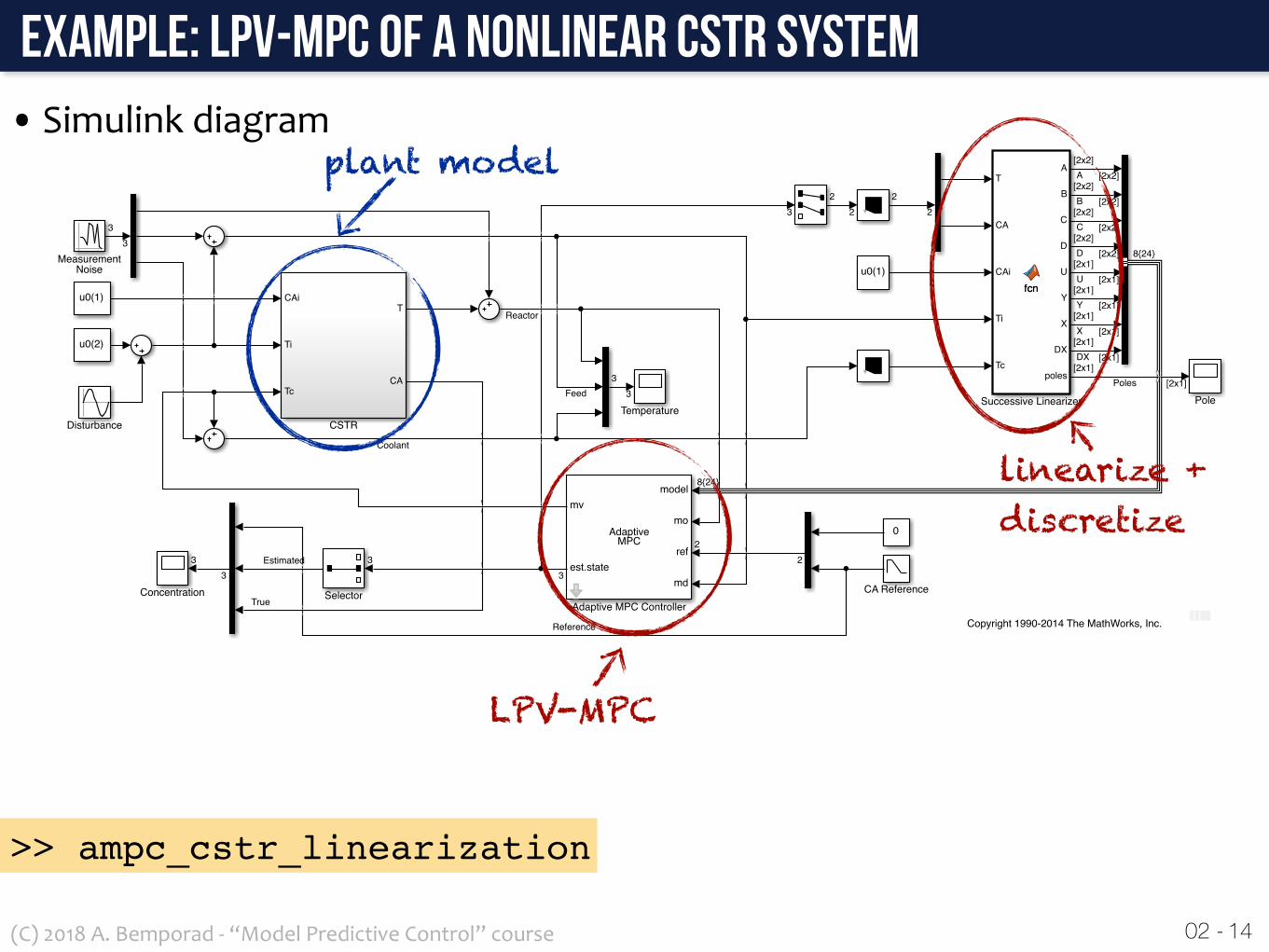
Example: LPV-MPC of a nonlinear CSTR system• Simulinkdiagram

14

>> ampc_cstr_linearization

plant model

LPV-MPC

linearize + discretize


Example: LPV-MPC of a nonlinear CSTR system•Closed-loopresults

15

Copyright 1990-2014 The MathWorks, Inc.Concentration

22

Temperature3

3

Noise

33

CA Reference

2

0

u0(1)

CAi

CAi

Ti

Tc

T

CA

CSTR

u0(2)

Ti

Disturbance

MPCmv

mo

ref

md

MPC Controller

2

Reference

Feed

Coolant

Reactor

True


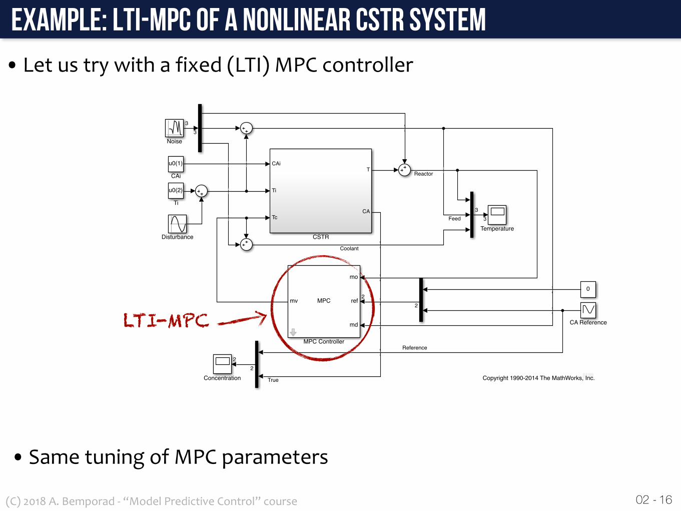
Example: LTI-MPC of a nonlinear CSTR system•Letustrywithafixed(LTI)MPCcontroller

16

LTI-MPC

•SametuningofMPCparameters


Example: LTI-MPC of a nonlinear CSTR system•Closed-loopresults

17

very bad tracking !


Example: LTI-MPC of a nonlinear CSTR system•Closed-loopresults

18

p(t) =⇥2

0

s2 + 2�⇥0s + ⇥20

pc(t)


Example: LTV-MPC for UAV navigation•Goal:navigatetwoplanarvehiclesamongobstaclestoatargetposition

•Thedynamicalmodelofeachvehiclesisdescribedby

19

p = [x,y]vehiclepositionpc = commandedposition

• Vehicledynamicsconvertedtodiscrete-timebyexactsampling

• Fivesquareobstaclesplacedinworkspace

• Goal:Uselineartime-varying(LTV)MPCtogeneratedesiredpositionstostabilizingcontrollerinreal-timetoavoidobstaclesandotherUAVs

• Problem:feasiblespaceisnon-convex!

• Mainidea:getaconvexinnerapproximationofthefeasiblespacethatis

– Polyhedral=linearconstraintsonpredictedstatesinLTV-MPCproblem

– Verysimpletocomputeon-line

– Canhandlepolytopicobstaclesofarbitraryshapeanddimension


LTV-MPC for obstacle avoidance

20

(Bemporad,Rocchi,IFAC2011)

• Alternative:non-convexfeasiblespacemodeledbymixed-integerconstraints,guidanceproblemsolvedby(time-invariant)hybridMPC

initial position

target position

p0 2 Rd = current vehicle position

q1, q2, . . . , qM 2 Rd = obstacle positions

p0 6= qi, 8i = 1, . . . ,MP =

8><

>:p 2 Rd :

2

64(q1 � p0)0

...(qM � p0)0

3

75 p

2

64(q1 � p0)0q1

...(qM � p0)0qM

3

75

9>=

>;


Fast greedy approximation algorithm (1/3)

21

• Polyhedralapproximation:

• Assume(forthemoment)thatvehicleandobstaclesarepointsinspace

• Pcontainsp0 anddoesnotcontainanyoftheobstaclesq1,q2,...,qM initsinterior

q1

qM

q2

p0

(Bemporad,Rocchi,CDC2011)

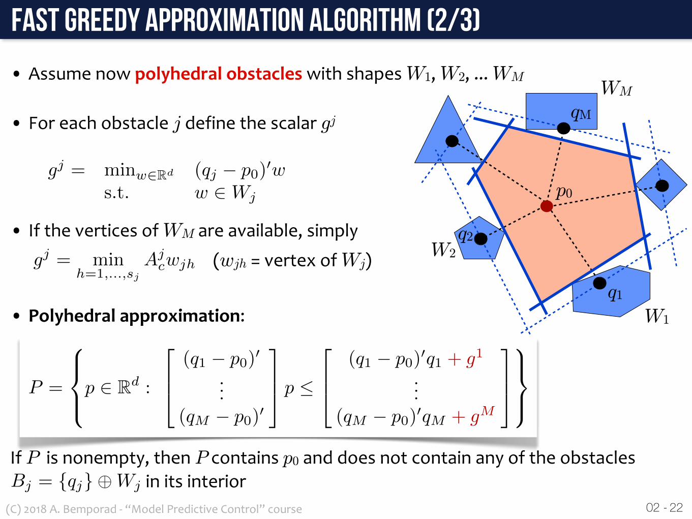
• IftheverticesofWMareavailable,simply

• AssumenowpolyhedralobstacleswithshapesW1,W2,...WM

gj = minw2Rd (qj � p0)0ws.t. w 2 Wj

gj = minh=1,...,sj

Ajcwjh

P =

8><

>:p 2 Rd :

2

64(q1 � p0)0

...(qM � p0)0

3

75 p

2

64(q1 � p0)0q1 + g1

...(qM � p0)0qM + gM

3

75

9>=

>;



22

IfPisnonempty,then Pcontainsp0 anddoesnotcontainanyoftheobstaclesinitsinterior

q1

qM

q2

p0

W2

W1

WM

• Foreachobstaclejdefinethescalar gj

Bj = {qj}�Wj

(wjh=vertexofWj)


• AssumepolyhedralobstaclesandpolytopicUAV

V

P =

8><

>:p 2 Rd :

2

64(q1 � p0)0

...(qM � p0)0

3

75 p

2

64(q1 � p0)0(q1 � di) + g1

...(qM � p0)0(qM � di) + gM

3

75 , i = 1, . . . , r

9>=

>;



23

q1

qM

q2

p0

W2

W1

WM

V , conv(p0 + d1, . . . , p0 + dr)

IfPisnonempty,then PcontainsV anddoesnotcontainanyoftheobstaclesinitsinteriorBj = {qj}�Wj


pi(t+ 1) = Aipi(t) +Bipci(t) pi(t) =

2

4xi(t)yi(t)zi(t)

3

5

V(t) = {p(t)}+ conv(d1(t), . . . , dr(t))

Bj(t) = {qj(t)}�Wj(t)


LTV-MPC guidance algorithm: prediction model

24

• LinearapproximationofstabilizeddynamicsofUAV#i

positionofvehicle#iattimet

• PolytopicshapeofUAV#i attimet

p(t) V(t)

• Polyhedralshapeofobstacle#j attimetqj(t)

Bj(t)

• Note:othervehiclesinformationaretreatedaspolytopicobstacles(Bj=V )

pci(t) =

2

4xci(t)yci(t)zci(t)

3

5positioncommandedattimet

Ac =

2

64(q1 � p0)0

...(qM � p0)0

3

75 , bc =

2

64(q1 � p0)0q1

...(qM � p0)0qM

3

75

min ⇢✏2 +

N�1X

k=0

kWy(pk � pd(t))k2 + kW�u(pc,k � pc,k�1)k2

s.t. pk+1 = Apk +Bpc,k, k = 0, . . . , N � 1

�min pc,k � pc,k�1 �max, k = 0, . . . , Nu � 1

Ac,kpk bc,k + gk �Ac,kdh,k +1I ✏

k = 0, . . . , N � 1, h = 1, . . . , ri

pc,k = pc,Nu�1, k = Nu, . . . , N


LTV-MPC guidance algorithm: optimization model

• Attimet,selectthedesiredpositionpc(t)fortheUAVbysolvingtheoptimalcontrolproblem(=quadraticprogramming)

prediction horizon

bounds on inputincrements

desired position

UAV dynamics

blocked moves

(soft)obstacleavoidanceconstraints


Example: navigation demo

26

• Initialposition#1=(0,0)• Targetposition#1=(35,30)

• Initialposition#2=(35,-3)• Targetposition#2=(0,20)

ROBMPC projectRobust Model Predictive Control (MPC) for Space Constrained Systems

(Bemporad,2010-2011)

MPCSofTToolboxforMATLAB


Example: navigation demo (cooperative MPC)•Twovehiclesavoidingeachotherandobstaclestowardstheirtargets

27

vehicle dynamics #1

vehicle dynamics #2

MPC #1

MPC #2

previous optimal sequences are exchanged

Linear Parameter Varying and Time-Varying Model Predictive...

Documents

Transcript of Linear Parameter Varying and Time-Varying Model Predictive...