Modeling and Forecasting the demand for Crude Oil in...
36
1 Modeling and Forecasting the demand for Crude Oil in Asian Countries By Dr. Nourah AbdulRahman Al-Yousef. PhD,MS,MBA,BA Associate professor Economic Department King Saud University e-mail: [email protected] PO. Box 85064 Riyadh 11691 Saudi Arabia Presented in 25 th USAEE/ IAEE North American Conference September 18 – 21, 2005 Omni Interlocken Resort, Denver, CO, USA Fueling The Future: Prices, Productivity, Policies and Prophesies
Transcript of Modeling and Forecasting the demand for Crude Oil in...
1
Modeling and Forecasting the demand for Crude Oil in Asian Countries
By
Dr. Nourah AbdulRahman Al-Yousef. PhD,MS,MBA,BA
Associate professor
Economic Department King Saud University
e-mail: [email protected]
PO. Box 85064 Riyadh 11691 Saudi Arabia Presented in
25th USAEE/ IAEE North American Conference September 18 – 21, 2005
Omni Interlocken Resort, Denver, CO, USA
Fueling The Future: Prices, Productivity, Policies and Prophesies
2
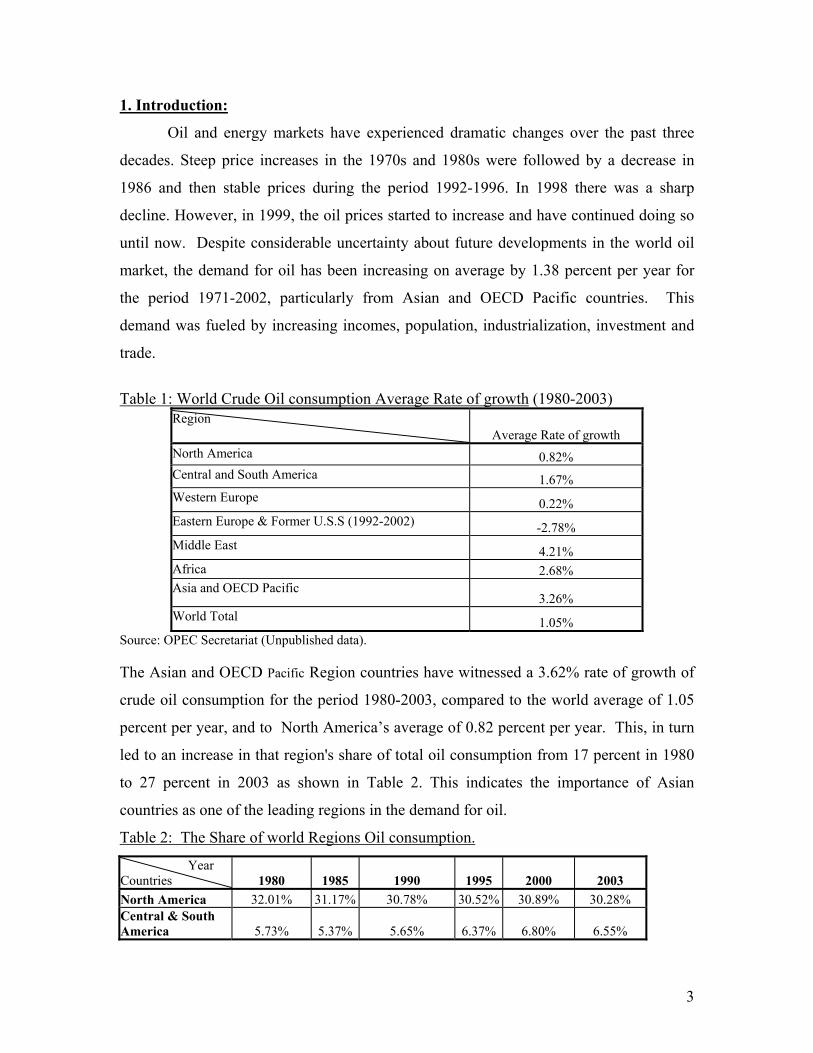
ABSTRACT
This study examines the growth in oil demand in selected Asian countries over the 1982-
2002 period. In particular, it analyses GDP and price in relation to oil demand. The
demand for crude oil imports for the Asian countries. Which will be divided into four
groups: first, Newly Industrializing Economics (NIEs) e.g. Hong Kong, Taiwan, Korea,
Singapore, Indonesia, Malaysia, the Philippines and Thailand, as one group; second,
OECD countries (Japan, and South Korea); Third is China fourth, South Asia (India and
Pakistan). These groups are divide according to geographical location and similitary of
economic status.
The demand function will be estimated using cointegration analysis and an Error
Correction Model (ECM). There are however, three approaches for estimating the ECM:
the Engle-Granger’s two-step procedure; General to specific Hendry's type of testing; and
the Autoregressive Distributed Lag (ARDL) approach of Pesaran et al. (1999, 2001).
First the stationarity for all the variables will be tested followed by the use of the
Autoregressive Distributed Lag (ARDL). This test has the advantage of its applicability
irrespective of the different integration level. The ARDL procedures involve two stages.
The first stage, is testing the existence of the long-run relation between the variables
using "the Bound testing approach" (Pesaran, et al 2001). The second stage of the
analysis is to estimate the coefficients of the long run relations and to make inferences
about their values using the ARDL approach. Finally, the ARDL model is used to
forecastle the crude oil consumption for the years 2006-2010. The paper concludes that
GDP and Price are significant variables in demand for oil. However, elasticities of
demand were low indicating the importance of Asia’s crude oil to the economies of the
Asian countries.
When the estimated model was used to forecast crude oil demand, it was found
that GDP growth is an essential factor in the increase or decrease of crude oil demand by
Asian countries. China has the largest demand for crude oil followed by Japan; South
Korea; NIEs; India and with Pakistan being last. Recently, China, India and Pakistan
show a high growth rate of oil demand.
3
1. Introduction:
Oil and energy markets have experienced dramatic changes over the past three
decades. Steep price increases in the 1970s and 1980s were followed by a decrease in
1986 and then stable prices during the period 1992-1996. In 1998 there was a sharp
decline. However, in 1999, the oil prices started to increase and have continued doing so
until now. Despite considerable uncertainty about future developments in the world oil
market, the demand for oil has been increasing on average by 1.38 percent per year for
the period 1971-2002, particularly from Asian and OECD Pacific countries. This
demand was fueled by increasing incomes, population, industrialization, investment and
trade.
Table 1: World Crude Oil consumption Average Rate of growth (1980-2003)
Region Average Rate of growth
North America 0.82% Central and South America 1.67% Western Europe 0.22% Eastern Europe & Former U.S.S (1992-2002) -2.78% Middle East 4.21% Africa 2.68% Asia and OECD Pacific
3.26% World Total 1.05%
Source: OPEC Secretariat (Unpublished data). The Asian and OECD Pacific Region countries have witnessed a 3.62% rate of growth of
crude oil consumption for the period 1980-2003, compared to the world average of 1.05
percent per year, and to North America’s average of 0.82 percent per year. This, in turn
led to an increase in that region's share of total oil consumption from 17 percent in 1980
to 27 percent in 2003 as shown in Table 2. This indicates the importance of Asian
countries as one of the leading regions in the demand for oil.
Table 2: The Share of world Regions Oil consumption.
Year Countries 1980 1985 1990 1995 2000 2003 North America 32.01% 31.17% 30.78% 30.52% 30.89% 30.28% Central & South America 5.73% 5.37% 5.65% 6.37% 6.80% 6.55%

4
Western Europe 22.69% 20.46% 19.99% 20.22% 19.06% 18.67% Eastern Europe & Former U.S.S.R. 16.97% 17.35% 14.62% 8.15% 6.62% 6.75% Middle East 3.26% 4.75% 5.25% 5.94% 6.21% 6.60% Africa 2.34% 3.04% 3.11% 3.22% 3.26% 3.37% Asia & Oceania 17.00% 17.86% 20.61% 25.58% 27.16% 27.79%
As illustrated on Figure 1, while Asia and Pacific consume less than 10.00 Mb/d in early
seventies, coming third after North America and Western Europe, Asia and Specific
countries consumption has continued to increase dramatically reaching a level of more
that 20 Mb/d in 1999 and has continued to increase to become second following North
American.
Figure 1: World demand for Crude Oil by Major Consumer (1980-2003)
0.0
5,000.0
10,000.0
15,000.0
20,000.0
25,000.0
30,000.0
1980
1981
1982
1983
1984
1985
1986
1987
1988
1989
1990
1991
1992
1993
1994
1995
1996
1997
1998
1999
2000
2001
2002
2003
Thou
sand
Bar
rel P
er
Day
North America Western Europe Asia & Oceania
2. The Objective of the study:
This study examines the growth in oil demand in selected Asian countries for the
period 1982-2002. In particular, it analyses GDP and price, in relations to the demand
for oil. An Econometric model of the regions’ demand for oil will be driven from a cost
minimization problem in which demand depends on the price of oil and the GDP. The
model includes estimation of short and long-term elasticities of demand. The study starts
with a historical overview of the growth in crude oil consumption. This is followed by a
5
review of the main economic indicators that effect crude oil demand, such as energy
efficiency and economic growth for each country that included in the study. Variables of
the study include Consumption of Crude oil, Real GDP in USA Dollar, and Crude oil
Price. The sources for data are OPEC secretariat and Energy Information Administration
(EIA). The data will cover the period 1980-2003 for the following countries: Japan,
South Korea, China, and NIEs countries as one group, In edition to South Asian
Countries India and Pakistan as the last group.
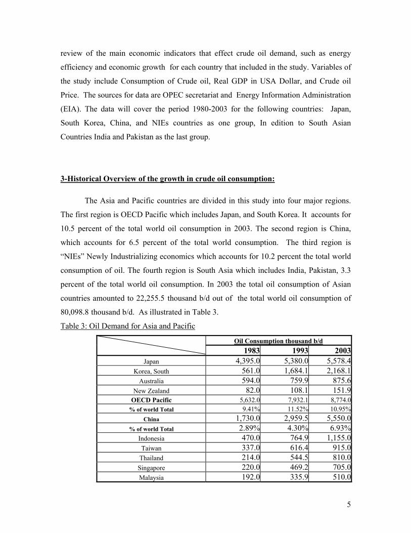
3-Historical Overview of the growth in crude oil consumption:
The Asia and Pacific countries are divided in this study into four major regions.
The first region is OECD Pacific which includes Japan, and South Korea. It accounts for
10.5 percent of the total world oil consumption in 2003. The second region is China,
which accounts for 6.5 percent of the total world consumption. The third region is
“NIEs” Newly Industrializing economics which accounts for 10.2 percent the total world
consumption of oil. The fourth region is South Asia which includes India, Pakistan, 3.3
percent of the total world oil consumption. In 2003 the total oil consumption of Asian
countries amounted to 22,255.5 thousand b/d out of the total world oil consumption of
80,098.8 thousand b/d. As illustrated in Table 3.
Table 3: Oil Demand for Asia and Pacific
Oil Consumption thousand b/d 1983 1993 2003
Japan 4,395.0 5,380.0 5,578.4Korea, South 561.0 1,684.1 2,168.1
Australia 594.0 759.9 875.6New Zealand 82.0 108.1 151.9
OECD Pacific 5,632.0 7,932.1 8,774.0% of world Total 9.41% 11.52% 10.95%
China 1,730.0 2,959.5 5,550.0% of world Total 2.89% 4.30% 6.93%
Indonesia 470.0 764.9 1,155.0Taiwan 337.0 616.4 915.0
Thailand 214.0 544.5 810.0Singapore 220.0 469.2 705.0Malaysia 192.0 335.9 510.0
6
Philippines 195.0 284.5 335.0Hong Kong 119.0 157.5 260.0
Vietnam 26.6 77.4 216.0Other Asia, Other 41.0 1,426.3 3,270.5
NIEs 1,814.6 4,676.7 8,176.5% of world Total 3.0% 6.8% 10.2%
India 824.0 1,413.3 2,320.0Pakistan 140.0 282.2 338.0
South Asia 964.0 1,695.4 2,658.0% of world Total 1.6% 2.5% 3.3%
Total Asian Countries 10,350.0 16,006.4 22,255.5% of World Total Oil Consumption 17.3% 23.2% 27.8%
World Total 59,829.6 68,845.7 80,098.8
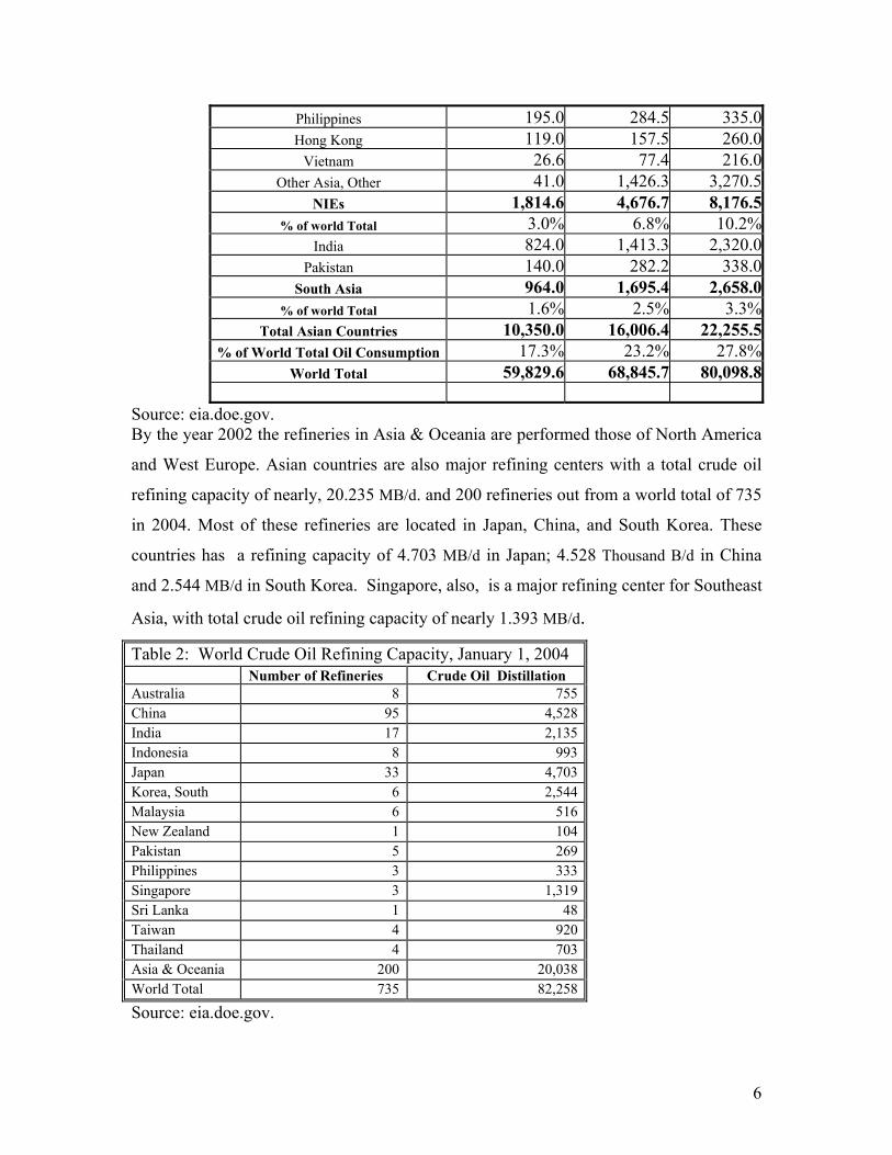
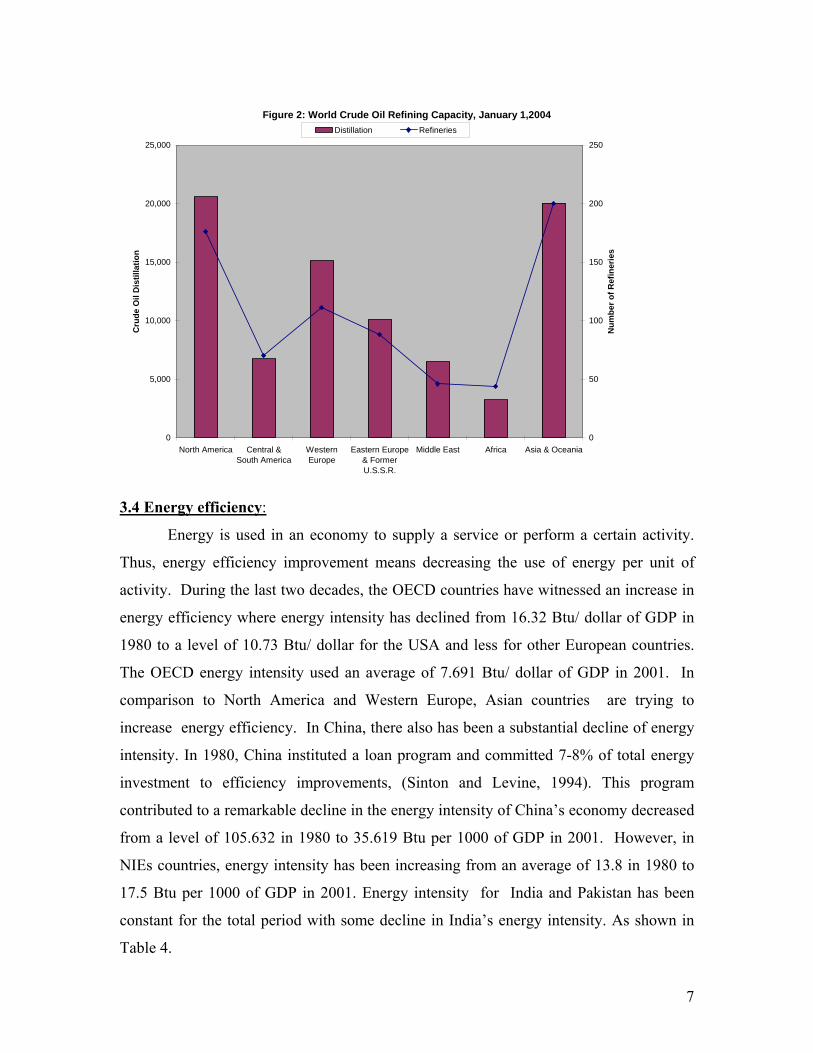
Source: eia.doe.gov. By the year 2002 the refineries in Asia & Oceania are performed those of North America
and West Europe. Asian countries are also major refining centers with a total crude oil
refining capacity of nearly, 20.235 MB/d. and 200 refineries out from a world total of 735
in 2004. Most of these refineries are located in Japan, China, and South Korea. These
countries has a refining capacity of 4.703 MB/d in Japan; 4.528 Thousand B/d in China
and 2.544 MB/d in South Korea. Singapore, also, is a major refining center for Southeast
Asia, with total crude oil refining capacity of nearly 1.393 MB/d.
Table 2: World Crude Oil Refining Capacity, January 1, 2004 Number of Refineries Crude Oil Distillation Australia 8 755China 95 4,528India 17 2,135Indonesia 8 993Japan 33 4,703Korea, South 6 2,544Malaysia 6 516New Zealand 1 104Pakistan 5 269Philippines 3 333Singapore 3 1,319Sri Lanka 1 48Taiwan 4 920Thailand 4 703Asia & Oceania 200 20,038World Total 735 82,258
Source: eia.doe.gov.
7
Figure 2: World Crude Oil Refining Capacity, January 1,2004
0
5,000
10,000
15,000
20,000
25,000
North America Central &South America
WesternEurope
Eastern Europe& FormerU.S.S.R.
Middle East Africa Asia & Oceania
Cru
de O
il D
istil
latio
n
0
50
100
150
200
250
Num
ber o
f Ref
iner
ies
Distillation Refineries
3.4 Energy efficiency:
Energy is used in an economy to supply a service or perform a certain activity.
Thus, energy efficiency improvement means decreasing the use of energy per unit of
activity. During the last two decades, the OECD countries have witnessed an increase in
energy efficiency where energy intensity has declined from 16.32 Btu/ dollar of GDP in
1980 to a level of 10.73 Btu/ dollar for the USA and less for other European countries.
The OECD energy intensity used an average of 7.691 Btu/ dollar of GDP in 2001. In
comparison to North America and Western Europe, Asian countries are trying to
increase energy efficiency. In China, there also has been a substantial decline of energy
intensity. In 1980, China instituted a loan program and committed 7-8% of total energy
investment to efficiency improvements, (Sinton and Levine, 1994). This program
contributed to a remarkable decline in the energy intensity of China’s economy decreased
from a level of 105.632 in 1980 to 35.619 Btu per 1000 of GDP in 2001. However, in
NIEs countries, energy intensity has been increasing from an average of 13.8 in 1980 to
17.5 Btu per 1000 of GDP in 2001. Energy intensity for India and Pakistan has been
constant for the total period with some decline in India’s energy intensity. As shown in
Table 4.

8
Table 3 : World Primary Energy Consumption Per Dollar of Gross Domestic Product, 1980-2001 ( Btu per 1995 U.S. Dollars Using Market Exchange Rates)
OECD Pacific China
1983 1993 2003 1983 1993 2003Australia 14,724 13,770 12,383 China 89,733 53,678 33,175Korea, South 12,377 15,631 14,739 NIS Asia countries Japan 4,728 4,507 4,605Indonesia 19,838 23,352 28,041New Zealand 12,377 15,631 14,739Taiwan 13,213 11,843 12,924Mean 11,052 12,385 11,616Thailand 12,944 16,651 22,158
SD 4358.433 5324.71 4804.491Singapore 17,274 19,204 18,727 Malaysia 16,556 21,366 23,267
South Asia 30,449 25,460Philippines 10,687 14,426 14,407
India 27,245 25,002 24,403Hong Kong 5,054 4,667 4,995Pakistan 24,699 27,725 24,932Vietnam 18,021 20,389 25,715Mean 25,972 3851.886 747.4419 Mean 14,198 16,487 18,779SD 1800.294 SD 5551.303 6878.237 8187.61
Source: Energy Information Administration www. eia.doe.gov
4. Economic Growth
For the past two decades, Asia has witnessed a remarkable economic growth. Asia grew
by an average of 5.30 percent with China growing by an average rate of 9.55 percent for
the period of 1980-2002. The average economic growth of these countries has
outperformed these of Western Europe.
For the period 1980-1995, the OECD countries in Asia (mainly Japan) were the
dominating economy in the region, with the main contributor to economic growth. The
“NIEs” start showing a high growth rate starting from 1986. This was followed by other
countries including Indonesia, Malaysia, the Philippines and Thailand. Table 5: Asian and specific countries’aِverage real Economic Growth (1980-2003).
2003-1980 Australia 3.53% China 9.56% Hong Kong 5.13% India 5.68% Indonesia 4.67% Japan 2.51% Korea, South 6.98%
9
Malaysia 6.14% New Zealand 2.82% Pakistan 4.85% Philippines 2.64% Singapore 6.53% Taiwan 6.45% Thailand 6.07% Vietnam 5.18%
Total Asia/Pacific 5.25% Source: International Monetary Statistics IMS
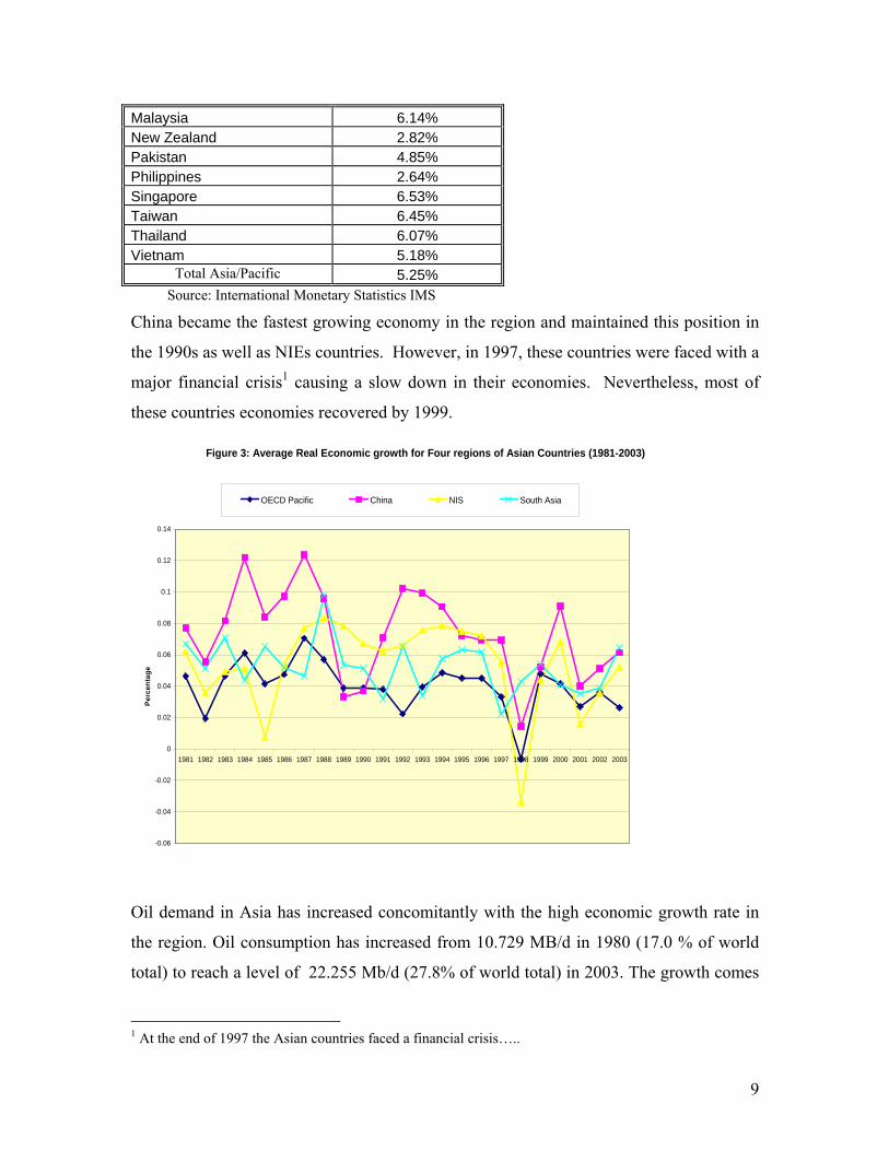
China became the fastest growing economy in the region and maintained this position in
the 1990s as well as NIEs countries. However, in 1997, these countries were faced with a
major financial crisis1 causing a slow down in their economies. Nevertheless, most of
these countries economies recovered by 1999.
Figure 3: Average Real Economic growth for Four regions of Asian Countries (1981-2003)
-0.06
-0.04
-0.02
0
0.02
0.04
0.06
0.08
0.1
0.12
0.14
1981 1982 1983 1984 1985 1986 1987 1988 1989 1990 1991 1992 1993 1994 1995 1996 1997 1998 1999 2000 2001 2002 2003
Perc
enta
ge
OECD Pacific China NIS South Asia
Oil demand in Asia has increased concomitantly with the high economic growth rate in
the region. Oil consumption has increased from 10.729 MB/d in 1980 (17.0 % of world
total) to reach a level of 22.255 Mb/d (27.8% of world total) in 2003. The growth comes
1 At the end of 1997 the Asian countries faced a financial crisis…..
10
mainly from NIEs, where it grew from 1.747 Mb/d (2.7%) in 1980 to 4.906 Mb/d (6.12
%) in 2004. China’s consumption increased from less than two millions in 1980(2.8%) to
reach 5.55(6.12%) MB/d in 2003. Each region’s economic growth will be explained in
the following section:
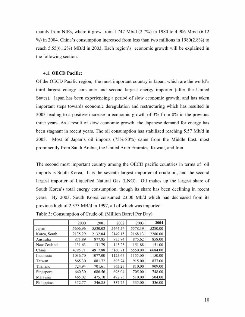
4.1. OECD Pacific:
Of the OECD Pacific region, the most important country is Japan, which are the world’s
third largest energy consumer and second largest energy importer (after the United
States). Japan has been experiencing a period of slow economic growth, and has taken
important steps towards economic deregulation and restructuring which has resulted in
2003 leading to a positive increase in economic growth of 3% from 0% in the previous
three years. As a result of slow economic growth, the Japanese demand for energy has
been stagnant in recent years. The oil consumption has stabilized reaching 5.57 Mb/d in
2003. Most of Japan’s oil imports (75%-80%) came from the Middle East. most
prominently from Saudi Arabia, the United Arab Emirates, Kuwait, and Iran.
The second most important country among the OECD pacific countries in terms of oil
imports is South Korea. It is the seventh largest importer of crude oil, and the second
largest importer of Liquefied Natural Gas (LNG). Oil makes up the largest share of
South Korea’s total energy consumption, though its share has been declining in recent
years. By 2003. South Korea consumed 23.00 Mb/d which had decreased from its
previous high of 2.373 MB/d in 1997, all of which was imported.
Table 3: Consumption of Crude oil (Million Barrel Per Day)
2000 2001 2002 2003 2004Japan 5606.96 5530.03 5464.56 5578.39 5280.00Korea, South 2135.29 2132.04 2149.15 2168.13 2280.00Australia 871.89 877.85 875.84 875.62 858.00New Zealand 131.63 131.79 145.25 151.88 151.00China 4795.71 4917.88 5160.71 5550.00 6684.00Indonesia 1036.70 1077.00 1125.65 1155.00 1150.00Taiwan 865.30 881.72 893.74 915.00 877.00Thailand 724.94 701.61 763.27 810.00 909.00Singapore 660.30 686.56 698.04 705.00 748.00Malaysia 465.02 475.10 492.75 510.00 504.00Philippines 352.77 346.85 337.75 335.00 336.00
11
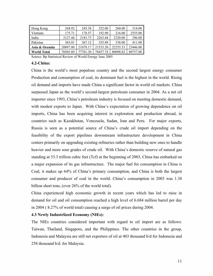
Hong Kong 244.92 245.38 252.00 260.00 314.00Vietnam 175.71 178.57 192.90 216.00 2555.00India 2127.44 2183.73 2263.44 2320.00 296.00Pakistan 365.01 367.12 355.89 338.00 411.00Asia & Oceania 20897.80 21078.17 21535.20 22255.53 23446.00World Total 76945.89 77701.30 78457.74 80098.82 80757.00Source: Bp Statistical Review of World Energy June 2005
4.2-China:
China is the world’s most populous country and the second largest energy consumer
Production and consumption of coal, its dominant fuel is the highest in the world. Rising
oil demand and imports have made China a significant factor in world oil markets. China
surpassed Japan as the world’s second-largest petroleum consumer in 2004. As a net oil
importer since 1993, China’s petroleum industry is focused on meeting domestic demand,
with modest exports to Japan. With China’s expectation of growing dependence on oil
imports, China has been acquiring interest in exploration and production abroad, in
countries such as Kazakhstan, Venezuela, Sudan, Iran and Peru. For major exports,
Russia is seen as a potential source of China’s crude oil import depending on the
feasibility of the export pipelines downstream infrastructure development in China
centers primarily on upgrading existing refineries rather than building new ones to handle
heavier and more sour grades of crude oil. With China’s domestic reserve of natural gas
standing at 53.3 trillion cubic feet (Tcf) at the beginning of 2003, China has embarked on
a major expansion of its gas infrastructure. The major fuel for consumption in China is
Coal, it makes up 64% of China’s primary consumption, and China is both the largest
consumer and producer of coal in the world. China’s consumption in 2003 was 1.38
billion short tons, (over 26% of the world total).
China experienced high economic growth in recent years which has led to raise in
demand for oil and oil consumption reached a high level of 6.684 million barrel per day
in 2004 ( 8.27% of world total) causing a surge of oil prices during 2004.
4.3 Newly Industrlized Economy (NIEs):
The NIEs countries considered important with regard to oil import are as follows:
Taiwan, Thailand, Singapore, and the Philippines. The other countries in the group,
Indonesia and Malaysia are still net exporters of oil at 403 thousand b/d for Indonesia and
258 thousand b/d. for Malaysia.

12
4.3.1 Taiwan: Taiwan is a leading economic and trading center. For Taiwan, oil is by far
the dominant fuel contribution, representing 51% of its total energy consumption. Coal
also plays an important role (32% of total energy consumption) followed by nuclear
power (8%) and natural gas (6%) Taiwan has very limited domestic energy resources and
relies on imports for most of its energy requirements.
4.3.2 Thailand: Thailand is a important energy consumer, and its energy consumption is
expected to resume strong growth as the country recovers from the global slow down of
2001-2002. In 2001, Thailand produced about 175,027 barrels per day of oil. It’s oil
consumption peaked in 1996 at 749,000 b/d. It fell to 706,000 in 1998 during the Asian
crisis, by 2001 it had increased to 715,000 b/d. Part of the reason consumption has not
recovered fully is that the Thai government has been raising taxes on petroleum products,
which is intended to promote conservation and reduce oil imports. However, by 2003 the
demand of oil increased to a level of 836000 b/d.
4.3.3. Singapore: Singapore is a major refining center for Southeast Asia, with total crude
oil refining capacity of nearly 1.3 Mb/d has nearly doubled its rate of petroleum products
consumption. It is also strategically located near the Strait of Malacca, a major route for
oil tankers. Singapore’s strategic location has helped it to become one of the most
important shipping centers in Asia. The Asian economic crisis of 1997-98 had a negative
impact on Singapore’s refining industry and Singapore’s refining companies lost
significant business due to the declining demand for oil products in the region. While the
region staged a recovery from the financial crisis in 1999 and 2000, the construction of
new refineries in Singapore’s traditional export markets has had a more enduring
negative effect.
4.3.4. The Philippine: The Philippines are a growing consumer of energy, particularly
electric power, and a major potential market for foreign energy firms. It’s also produce a
modest amount of less than 9 thousand Barrel/d while it consumes 356 thousand B/d
resulting in net imports of 347 thousand. On the other hand, the Philippines have 3.693
trillion cubic feet of gas proven reserves but no significant production at the present time.
4.3.5 Indonesia: Indonesia is important to world energy markets since it is the only NIEs
member of OPEC and it is the worlds largest liquefied natural gas (LNG) exporter.
13
Indonesia currently holds proven reserves of 5 billion barrels. In 2003, Indonesian crude
oil production averaged 1.24 million barrels per day B/d, having decreased from its pick
at 1.638 Mb/d in 1995. The recent declines in production are due mainly to a natural
decline of aging oil fields, which recent oil discoveries have been too small to offset.
Besides crude oil, Indonesia also produces approximately 230,000 b/d of natural gas
liquids and lease condensate (which are not part of OPEC quota) bringing the country’s
total oil production to around 1.3 Mb/d. Despite the significant proven natural gas
reserve of 92.5 trillion cubic feet (Tef) and its position as the world’s largest exporter of
LNG, Indonesia still relies on oil to supply about half of its energy needs. About 70% of
Indonesia’s LNG exports are to Japan, 20% to South Korea, and the remainder to
Taiwan. As Indonesia’s oil production has leveled off in recent years, the country has
tried to shift towards using its natural gas resources for power generation. However, the
domestic natural gas distribution infrastructure is still not extensive.
4.3.6 Malaysia: Malaysia holds 75.0 trillion cubic feet (tcf) of natural gas reserves and 3
billion barrel of oil reserves. Its oil exports average 260,000 barrels per day and its LNG
exports 0.74 tcf. Despite its declining oil reserves (due to a lack of major new discoveries
in recent years), Malaysia’s crude oil production has been stable in recent years, between
650-730 thousand b/d. Its domestic product consumption is growing again. Moreover,
the country is expected to become a net oil importer before the end of the current
decades. Malaysia has six refineries with a total processing capacity of 516 B/d. Natural
gas production has been raising steadily in recent years, reaching 1.7 tcf in 2000, up from
1.42 tcf in 1999.
4.4 South Asia:
South Asia countries consist of India, Pakistan, Afghanistan, Pangldish, Sri Lanka Nepal
and Kashmir among others. However, India and Pakistan are the two most important
economies in the region. Moreover both are the major consumers of oil in the region of
South Asia.
4.4.1 India: India is the world’s sixth largest energy consumer and is planning major
energy infrastructure investments to keep up with increasing demand-particularly for
electric power. India is also the world’s third largest producer of coal which satisfies

14
more than half of its total energy needs. Oil accounts for about 30% of India’s total
energy consumption. India has implemented a series of policy changes since the mid-
1990s to encourage foreign investment which is expected to grow rapidly, beyond the
level of 1.5 in 2001. India is attempting to limit its dependence on oil import somewhat
by expanding domestic exploration and production.
4.4.2 Pakistan: Pakistan produced 61 thousand B/d of oil in 2003, and consumed 338
Thousand b/d. This means they had a net total of oil imports of 276 thousand b/d.
Pakistan’s net imports are projected to rise substantially in the coming years as demand
outpaces the increase in production. The demand for refined petroleum products also
greatly exceeds domestic oil refining capacity, so nearly half of Pakistan imports are
refined products.
Section 4, indicates the importance of Asian Countries as a major consumer of oil. Even
though, several countries produce oil they become by the 1995 net importer. Only
Indonesia and Vietnam still produce more than it consume. Japan followed by China (in
the year 2001) is the major consumer of oil in the Asian countries. However, China is the
second oil consumer now with its high economic growth causing oil prices to surge in
2004. Moreover, there growing economies are indicating the major role that they are
playing in the world oil marker. This role will have more significant on the coming years.
Table 7: Total Consumption, Production and Imports of Asian and Pacific countries (2003)Thousands Barrel a Day. Consumption Production Import Japan 5578.39 120.7 5457.7Korea, South 2168.13 2.8 2165.3Australia 875.62 630.8 244.9New Zealand 151.88 31.7 120.1China 5550.00 3,549.0 2001.0Indonesia 1155.00 1,240.0 *(-85.0)Taiwan 915.00 8.4 906.6Thailand 810.00 255.5 554.5Singapore 705.00 8.3 696.7Malaysia 510.00 840.3 *(-330.3)Philippines 335.00 14.4 320.6Hong Kong 260.00 0 260.0India 2320.00 814.9 1505.1Pakistan 2320.00 61.9 2258.1Vietnam 338.00 352.5 *(-14.5)
15
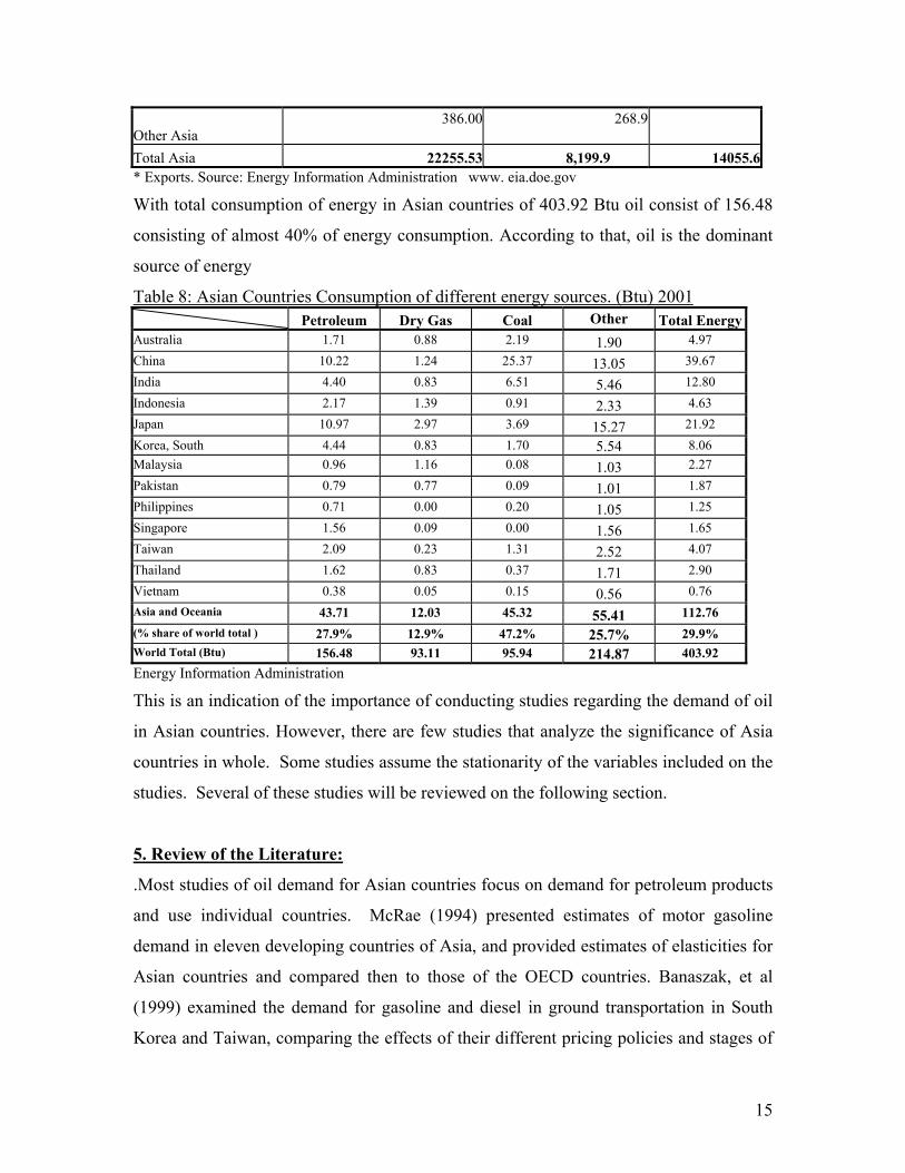
Other Asia 386.00 268.9
Total Asia 22255.53 8,199.9 14055.6* Exports. Source: Energy Information Administration www. eia.doe.gov
With total consumption of energy in Asian countries of 403.92 Btu oil consist of 156.48
consisting of almost 40% of energy consumption. According to that, oil is the dominant
source of energy
Table 8: Asian Countries Consumption of different energy sources. (Btu) 2001 Petroleum Dry Gas Coal Other Total EnergyAustralia 1.71 0.88 2.19 1.90 4.97 China 10.22 1.24 25.37 13.05 39.67 India 4.40 0.83 6.51 5.46 12.80 Indonesia 2.17 1.39 0.91 2.33 4.63 Japan 10.97 2.97 3.69 15.27 21.92 Korea, South 4.44 0.83 1.70 5.54 8.06 Malaysia 0.96 1.16 0.08 1.03 2.27 Pakistan 0.79 0.77 0.09 1.01 1.87 Philippines 0.71 0.00 0.20 1.05 1.25 Singapore 1.56 0.09 0.00 1.56 1.65 Taiwan 2.09 0.23 1.31 2.52 4.07 Thailand 1.62 0.83 0.37 1.71 2.90 Vietnam 0.38 0.05 0.15 0.56 0.76 Asia and Oceania 43.71 12.03 45.32 55.41 112.76 (% share of world total ) 27.9% 12.9% 47.2% 25.7% 29.9% World Total (Btu) 156.48 93.11 95.94 214.87 403.92 Energy Information Administration This is an indication of the importance of conducting studies regarding the demand of oil
in Asian countries. However, there are few studies that analyze the significance of Asia
countries in whole. Some studies assume the stationarity of the variables included on the
studies. Several of these studies will be reviewed on the following section.
5. Review of the Literature:
.Most studies of oil demand for Asian countries focus on demand for petroleum products
and use individual countries. McRae (1994) presented estimates of motor gasoline
demand in eleven developing countries of Asia, and provided estimates of elasticities for
Asian countries and compared then to those of the OECD countries. Banaszak, et al
(1999) examined the demand for gasoline and diesel in ground transportation in South
Korea and Taiwan, comparing the effects of their different pricing policies and stages of
16
economic growth. Han, X. and Lakshmanan, T., (1994) analyzed the effects of the
pervasive changes in the Japanese economy on its energy intensity during the period
1975-85. Fatai. K et al (2003) modeled and forecasted the demand for electricity in New
Zealand and compared alternative approaches.
Other studies used demand for energy not specific energy source, Lee and Hing (1997)
used Co integration and vector error-correction model to analyze the energy consumption
behavior in China. They found that not only convention variables such as energy price
and income are important. Galli, R (1998) studied the relationship between energy
intensity and income levels and forecasted long-term energy demand in Asian emerging
countries for the period 1973-1990 using a quadric function of log income. Kenneth, et al
(2001) examines the relationship between economic development and energy demand
and analyzed the effect of sector-specific energy demand growth rates on the composition
of fuel energy demand, for selected Developing countries.
In another paper comparing the dependence on the Gulf oil regarding the importance of
Asian-Pacific, region oil vs. the US Salameh (2003) analyzed the impact of growing
dependence of Asian Pacific region on the Gulf oil.
In the literature, number of studies have used Granger Causality to analyze the
relationship between consumption GDP and oil price, Masih et al (1996) used System
equations to test the relationship between consumptions and real income for six Asian
countries While Cheng et al (1997) applied Granger causality between energy
consumption and GDP using techniques of co integration to Taiwanese data for the 1955-
1993 period. Asafu-Adjaye (2000) estimates the causal relationships between energy
consumption and income for India, Indonesia, Philippines and Thailand. Using
cointegration and error-correction modeling techniques. The results indicate that in the
short run Granger causality is unidirectional, running from energy to GDP for India and
Indonesia. Masih, A. et al (1997) tested for cointegration between total energy
consumption, real income, and price level of two highly energy dependent East-Asian
NIEs: Korea and Taiwan. The Granger causality was tested using a dynamic vector
correction model. Masih, A et al (1997) concluded that it is the rate of price change that
leads to the change in energy consumption, which leads on to the change in economic
growth.
17
In this paper crude oil demand will be estimated for the Asian countries which
include NIEs Countries (Singapore, Thailand, Taiwan Philippine and Other East Asian
countries) as one group , OECD countries (Japan, South Korea), China, India and
Pakistan., using co integration analysis and an ECM. There are however three approaches
to estimating the ECM: the Engle-Granger’s two-step procedure and Hendry's type of
testing down., and the Autoregressive Distributed Lag (ARDL) approach of Pesaran et
al.. (1999, 2001). To avoid "spurious result" stationarity all variables will be tested and if
the variables are non-stationary, cointegration analysis and Error Correction Model will
be applied.
6. Method of Analysis:
The data commonly used in demand analysis is normally non-stationary; Plosser (1964)
Hendery 1982) among others indicated that econometric studies that overlook this
particular characteristic may get a "spurious result" i.e. giving parameters that is far from
the true one, also is leading to a very high R2 although there is nor relationship existing
between the variables included in the study. This problem occurs because both the
dependent and independent variables exhibit strong trends; the high R2 observed is due to
the presence of the trends, not to a true relationship between them.
To overcome the 'spurious' problem Engel and Granger (1986) show that one of the best
solutions is to apply co integration and error correction models (ECM). The advantages
of employing ECMs are numerous (see Bentzen and Engsted, 1993).
6.1 Cointegration and Error Correction Model
To illustrate the ECM model we use the following equilibrium equation:
tt xy βα += 1
yt is a dependent variable and xt is a vector of independent variables. If yt and xt
are in equilibrium, then the balance tt xy βα +− will equal zero. However, tt xy βα +−
will be non-zero when disequilibrium occurs. More precisely, this quantity measures the
extent of disequilibrium between yt and xt and hence is be assumed to be related to the
value of xt and the lagged values of yt and xt of which one typical form of which is
ttttt uyxxy ++++= −− 12110 δδδγ 2
18
Where ut is the disturbance term, subtracting yt-1 from both sides of Eq. (2) and
regrouping the resulting equation yields
ttttt uxyxy +−−−∆=∆ −− )( 110 βαµδ 3
Where µ, α and β assume the values 1-δ2, γ/ (1- δ2) and (δ0+ δ1)/ (1- δ2)
respectively. ∆ represents the first difference of the variables. Eq.(3) shows that the
change in yt depends on the change in xt and the lagged value of the disequilibrium error,
which implies that when yt-1 is greater than its equilibrium value, the value of yt will be
decreased for the disequilibrium error and hence is called the ECM. From Eq. (3), it is
clear that δ0 and β measures the short-run and long run parameters, while µ measures the
speed of adjustment towards the long-run equilibrium. Assuming a simple relationship in
Eq. 2, in practice Eq (2) is added with higher lag orders as explanatory variables, so as to
make ut white noise. When higher order lagged variables are introduced, Eq. (3) is
required to be modified into the form
tktkt
k
itt
k
itt uxyxyy +−−−∆+Ψ∆=∆ −−
−
=
−
=− ∑∑ )(
1
0
1
11 βαµδ (4)
The popularity of the ECM is due to the works of Granger (1983, 1988), Engle,
and Granger (1987) on cointegration. The importance of cointegration comes from the
fact that statistical inference from conventional regression is only valid when the
variables in a model are stationary. Most economic regression is only valid when
variables in a model are stationary. Most economic time series which are not stationary
leads to misspecification. To confront this problem, Engle and Granger develop the
concept of co integration. They argued that although the variables are individually non-
stationary a linear combination of the variables may be stationary. If this is the case, the
variables are said to be co integrated.
The relationship of the ECM to co integration analysis derives from a
representation theorem proved by Engle and Granger (1987). The theorem states that if
variables are cointegrated, then the short-run or disequilibrium can always be represented
by an ECM. Further, under the co integration assumptions, simple regressions will
provide a consistent estimates of the long-run coefficients, regardless of the variables are
correlated with the disturbances (thus causing ' simultaneous equation bias' in finite
samples' After 1988, however, a maximum-likelihood procedure developed by Johansen
19
and Juselius (1990) and Johansen (1991) began to replace the simple regression approach
to estimate the long-run coefficients. Due to Engle and Granger’s findings, both the
long-and short-run effects can be captured with the help of the ECM and counteraction
analysis.
6.2 Unit Root Tests
Before conducting the Engle-Granger ECM analysis, it is necessary to examine time
series properties of the variables to be estimated. This is important because if the
variables are non-stationary as well as non-co integrated; an ordinary least squares (OLS)
regression of Eq. (5) will be miss-specified, resulting in misleading values of R2, F and t
statistics. To investigate this, we conduct Augmented Dickey-Fuller (ADF) (1981) unit
root tests on the stationary of levels and the first differences of the variables included in
the study. In essence, testing whether a particular series, say zt, is integrated is equivalent
to testing for the significance of θ2, I.e. H0:θ2=0, in the regression below where T is a
linear trend.
t
k
iittt vzzTz ++++=∆ ∑
=−−
11210 λθθθ (5)
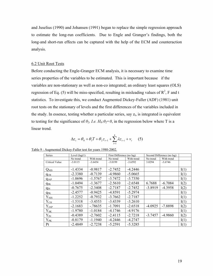
Table 9 : Augmented Dickey-Fuller test for years 1980-2002. Series Level (lag(1) First Difference (no lag) Second Difference (no lag) No trend With trend No trend With trend No trend With trend Critical Value -3.0115 -3.6454 -3.0199 -3.6592 3.0294
-3.6746
QNIS -1.4334 -0.9817 -2.7452 -4.2446 I(1) qCH -2.3380 -0.7139 -4.9860 -5.0665 I(1) qJAP -1.0696 -1.5767 -3.7472 -3.7350 I(1) qSK -1.0494 -1.3677 -2.5610 -2.6548 6.7688 -6.7084 I(2) qIN -0.7675 -2.3408 -2.7187 -2.7452 -3.8919 -4.3958 I(2) qPK -2.4577 -0.9425 -4.8591 -5.2974 I(1) YNIS -1.2252 -0.7932 -3.7662 -2.7187 I(1) YCH -1.5318 -3.4553 -3.4339 -3.2610 I(1) YJAP -2.1683 -.78635 -1.7091 -2.6518 -4.0925 -7.8898 I(2) YSK -1.9780 -1.0184 -4.1746 -4.9176 I(1) YIN -0.4389 -2.7602 -2.4115 -2.7218 -3.7457 -4.9860 I(2) YPK -0.8179 -1.1940 -4.2446 -4.2747 I(1) Pt -2.4849 -2.7238 -5.2591 -5.3285 I(1)
20
The results in Table 9 indicate that the variables under examination are integrated of
order one except those for South Korea, India and the GDP for Japan and China) which
indicate they are of order two I(2).
The result of the ADF test show that the time series included in the study has a
different order of integration therefore, we cannot use the Johansen Procedures which
require the equality of the level of integration. Hence, Autoregressive Distributed Lag
(ARDL) approach of Pesaran et al. (1999, 2001) will be used. It has the advantage of its
applicability irrespective of the different integration level. The ARDL procedures involve
two stages, First, testing the existence of the long run relation between the variables using
"the Bound testing approach" Pesaran, et al (2001). The second stage of the analysis is to
estimate the coefficients of the long run relations and make inference about their values
using the ARDL approach and testing the performance of the model in forecasting.
Finally, the ARDL model will be used in forecasting for the crude oil consumption for
the years 2003-2006.
Variables of the study include Consumption of Crude oil, Real GDP in USA
Dollar, and Crude oil Price. The data will cover the period 1980-2002. The source for the
data is OPEC secretariats.
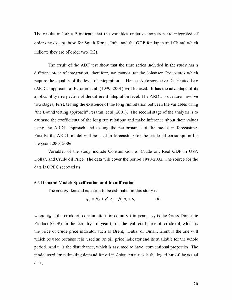
6.3 Demand Model: Specification and Identification
The energy demand equation to be estimated in this study is
ttitit upyq +++= 210 βββ (6)
where qit is the crude oil consumption for country i in year t, yit is the Gross Domestic
Product (GDP) for the country I in year t, p is the real retail price of crude oil, which is
the price of crude price indicator such as Brent, Dubai or Oman, Brent is the one will
which be used because it is used as an oil price indicator and its available for the whole
period. And ut is the disturbance, which is assumed to have conventional properties. The
model used for estimating demand for oil in Asian countries is the logarithm of the actual
data,
21
Lowercase letters denote the natural logarithm of variables and each coefficient estimated
as an elasticity. The data set contains annual observation over the period 1980-2002. The
source of the data is OPEC secretariats in Vienna and the Energy Information
Administration (EIA) in Washington, and it's provided in Appendix I. In order to
evaluate the forcastability of the model, it is run between the years 1980-1998, leaving
the last four observation period 1999-2002 for carrying out the post-sample forecast error
comparison. The estimation will be for different region: Japan; South Korea; China; NIEs
countries (which include Singapore, Thailand, Vietnam, and Taiwan, Philippine), and
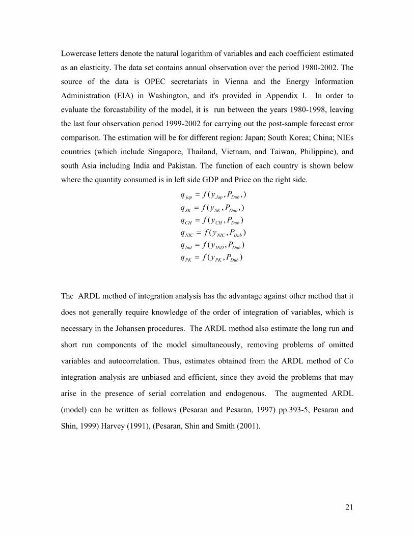
south Asia including India and Pakistan. The function of each country is shown below
where the quantity consumed is in left side GDP and Price on the right side.
),(),(),(
),(),,(
),,(
DubPKPK
DubINDInd
DubNICNIC
DubCHCH
DubSKSK
DubJapjap
PyfqPyfqPyfq
PyfqPyfq
Pyfq
=====
=
The ARDL method of integration analysis has the advantage against other method that it
does not generally require knowledge of the order of integration of variables, which is
necessary in the Johansen procedures. The ARDL method also estimate the long run and
short run components of the model simultaneously, removing problems of omitted
variables and autocorrelation. Thus, estimates obtained from the ARDL method of Co
integration analysis are unbiased and efficient, since they avoid the problems that may
arise in the presence of serial correlation and endogenous. The augmented ARDL
(model) can be written as follows (Pesaran and Pesaran, 1997) pp.393-5, Pesaran and
Shin, 1999) Harvey (1991), (Pesaran, Shin and Smith (2001).
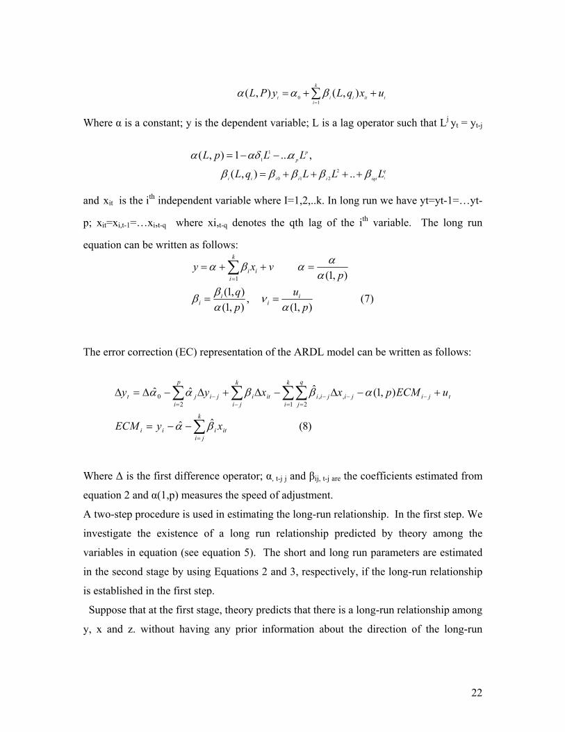
22
Where α is a constant; y is the dependent variable; L is a lag operator such that Lj yt = yt-j
and xit is the ith independent variable where I=1,2,..k. In long run we have yt=yt-1=…yt-
p; xit=xi,t-1=…xi,t-q where xi,t-q denotes the qth lag of the ith variable. The long run
equation can be written as follows:
)7(),1(
,),1(),1(
),1(1
pu
pq
pvxy
ii
ii
i
k
ii
αν
αββ
αααβα
==
=++= ∑=
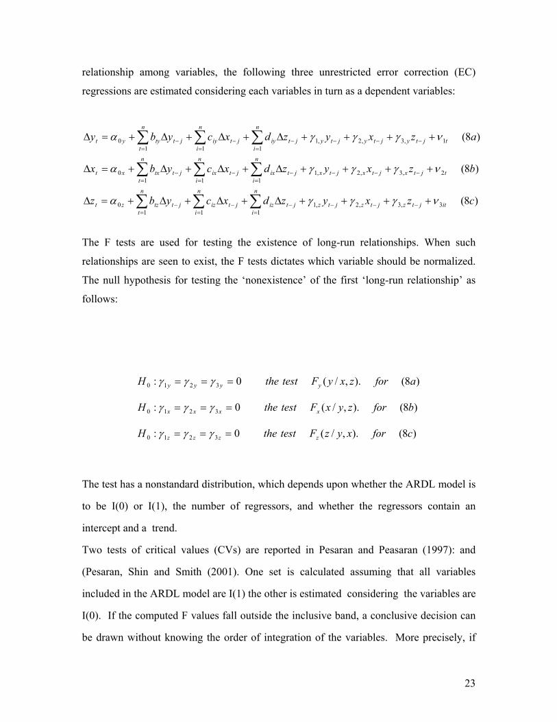
The error correction (EC) representation of the ARDL model can be written as follows:
)8(ˆˆ
),1(ˆˆˆ ,1 2
,2
0
it
k
jiiii
tjiji
k
i
q
jjiiit
k
jiiji
p
ijt
xyECM
uECMpxxyy
∑
∑∑∑∑
=
−−= =
−−
−=
−−=
+−∆−∆+∆−∆=∆
βα
αββαα
Where ∆ is the first difference operator; α, t-j j and βij, t-j are the coefficients estimated from
equation 2 and α(1,p) measures the speed of adjustment.
A two-step procedure is used in estimating the long-run relationship. In the first step. We
investigate the existence of a long run relationship predicted by theory among the
variables in equation (see equation 5). The short and long run parameters are estimated
in the second stage by using Equations 2 and 3, respectively, if the long-run relationship
is established in the first step.
Suppose that at the first stage, theory predicts that there is a long-run relationship among
y, x and z. without having any prior information about the direction of the long-run
01
( , ) ( , )k
t i i it ti
L P y L q x uα α β=
= + +∑
11
20 1 2
( , ) 1 ... ,
( , ) .. i
pp
qi i i i i iqi
L p L L
L q L L L
α αδ α
β β β β β
= − −
= + + + +
23
relationship among variables, the following three unrestricted error correction (EC)
regressions are estimated considering each variables in turn as a dependent variables:
)8(
)8(
)8(
3,3,2,1111
0
2,3,2,1111
0
1,3,2,1111
0
czxyzdxcybz
bzxyzdxcybx
azxyzdxcyby
itjtzjtzjtzjt
n
iizjt
n
iizjt
n
ttzzt
tjtxjtxjtxjt
n
iixjt
n
iixjt
n
ttxxt
tjtyjtyjtyjt
n
iiyjt
n
iiyjt
n
ttyyt
νγγγα
νγγγα
νγγγα
++++∆+∆+∆+=∆
++++∆+∆+∆+=∆
++++∆+∆+∆+=∆
−−−−=
−=
−=
−−−−=
−=
−=
−−−−=
−=
−=
∑∑∑
∑∑∑
∑∑∑
The F tests are used for testing the existence of long-run relationships. When such
relationships are seen to exist, the F tests dictates which variable should be normalized.
The null hypothesis for testing the ‘nonexistence’ of the first ‘long-run relationship’ as
follows:
)8().,/(0:
)8().,/(0:
)8().,/(0:
3210
3210
3210
cforxyzFtesttheH
bforzyxFtesttheH
aforzxyFtesttheH
zzzz
xxxx
yyyy
===
===
===
γγγ
γγγ
γγγ
The test has a nonstandard distribution, which depends upon whether the ARDL model is
to be I(0) or I(1), the number of regressors, and whether the regressors contain an
intercept and a trend.
Two tests of critical values (CVs) are reported in Pesaran and Peasaran (1997): and
(Pesaran, Shin and Smith (2001). One set is calculated assuming that all variables
included in the ARDL model are I(1) the other is estimated considering the variables are
I(0). If the computed F values fall outside the inclusive band, a conclusive decision can
be drawn without knowing the order of integration of the variables. More precisely, if

24
the empirical analysis shows that the estimated Fy(.) is higher than the upper bound of
the CV while Fx(.) and Fz(.) are lower than the lower bound of the CV, there exists a
‘unique and stable long run’ relationship. In this relationship, y is a dependent variable
and x and z are long run forcing’ or exogenous variables. Conversely, if the computed F
statistics fall within the band, prior information on the order of integration of the
variables is necessary to make a decision on the long-run relationship.
7. Results
Since the observations are annually, the maximum order of the lags used in the ARDL
model will be (2) and the estimation will be carried for the period 1980-1998, retaining
the remaining four years, 1999-2002 for predication.
The error correction version of the ARDL model in the variables lqit,lyit, and lpt is given
by:.
tkttkt
kk
itt
k
ikitt
k
ikitit
ylylq
lplylqlq
νγγγ
δϕα
++++
∆+∆+Ψ∆+=∆
−−−
=
=−
=
=−
=
=− ∑∑∑
3121
01
4
0
4
1 9
The Null hypothesis that will be tested is "non-existence of the long-run relationship"
defined by
0:0:
321
3210
≠≠≠===
γγγγγγ
AHH
10
Intercept and no trend, k=2 Long Run Relationship Critical values bounds 95% (3.79-4.85)
F-statistic (lqit/lyit,lpt)
F-statistic (lyit/lqit,lpt)
F-statistic (lpt/lyitlqit)
NIEs Countries 9.3863 3.4297 2.5323
Japan 1.5718 16.0350 3.4661 South Korea 2.0010 4.0273 1.7141 China 3.0492 3.0544 4.3643 India 0.71155 2.1906 1.7519 Pakistan 1.3560 1.3934 0.9872
K= number of regressors
The above test results suggest that there exists a long run relationship between lqit lyit,
and lpt, and that the variables lyit, and lpt can be treated as "long-run forcing" variables
25
for the explanation of lqit for all of the six region. This is because the F-statistic
(lqit/lyit,lpt) for all the six region either exceeds the upper bound of the critical value band
or less than the lower bound of the critical value band. Hence, we can reject the null of
no long run relationship between lqit lyit, and lpt . This, indicate the existence of
equilibrium relation between the three variables. The GDP and oil prices are significant
factors on the decision of consumption of oil on the long run and any changes in any of
the two variables will have emphasis on demand of oil.
For F-statistic (lyit/lqit,lpt)all the statistics fall well below the lower bound except for
this of South Korea, These result suggest that there exists a long run relationship between
lqit lyit, and lpt .
For F-statistic (lpt/lyitlqit) all the statistics fall well below the lower bound except for
China, These result suggest that there exists a long run relationship between lqit lyit, and
lpt . and the Variables lyit, and lpt can be treated as "the long Run forcing variables for the
explanation of lqit.
Table 10-15 : Error Correction model for NIEs, China, Japan, South Korea, India, Pakistan
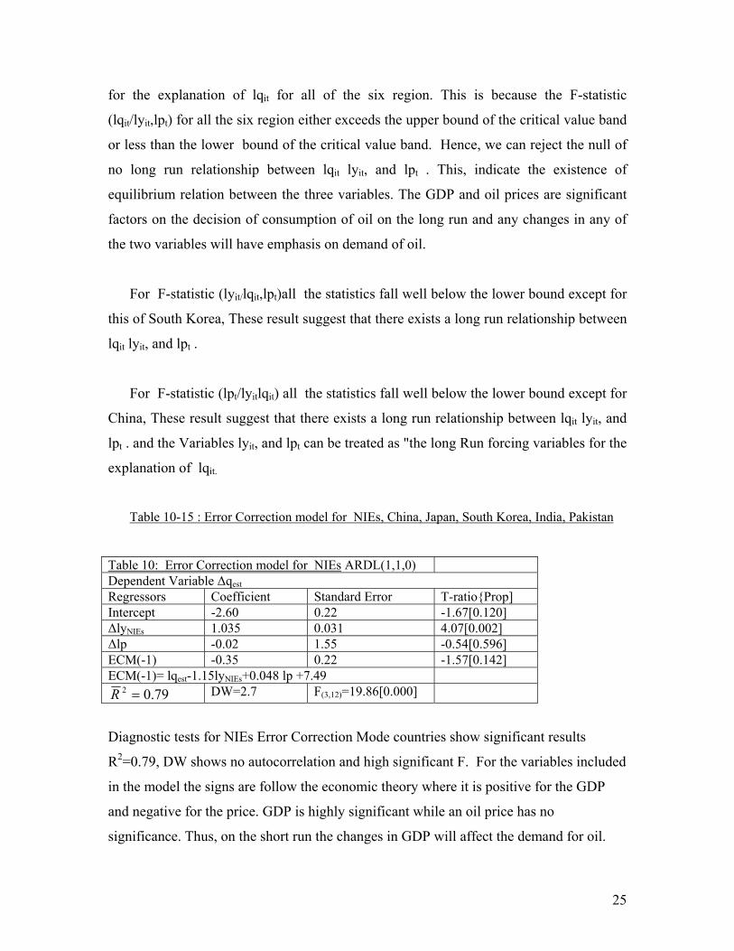
Table 10: Error Correction model for NIEs ARDL(1,1,0) Dependent Variable ∆qest Regressors Coefficient Standard Error T-ratio{Prop] Intercept -2.60 0.22 -1.67[0.120] ∆lyNIEs 1.035 0.031 4.07[0.002] ∆lp -0.02 1.55 -0.54[0.596] ECM(-1) -0.35 0.22 -1.57[0.142] ECM(-1)= lqest-1.15lyNIEs+0.048 lp +7.49
79.02 =R DW=2.7 F(3,12)=19.86[0.000]
Diagnostic tests for NIEs Error Correction Mode countries show significant results
R2=0.79, DW shows no autocorrelation and high significant F. For the variables included
in the model the signs are follow the economic theory where it is positive for the GDP
and negative for the price. GDP is highly significant while an oil price has no
significance. Thus, on the short run the changes in GDP will affect the demand for oil.
26
However, the price of oil will not have a significant effect on the demand for oil in NIEs
countries.
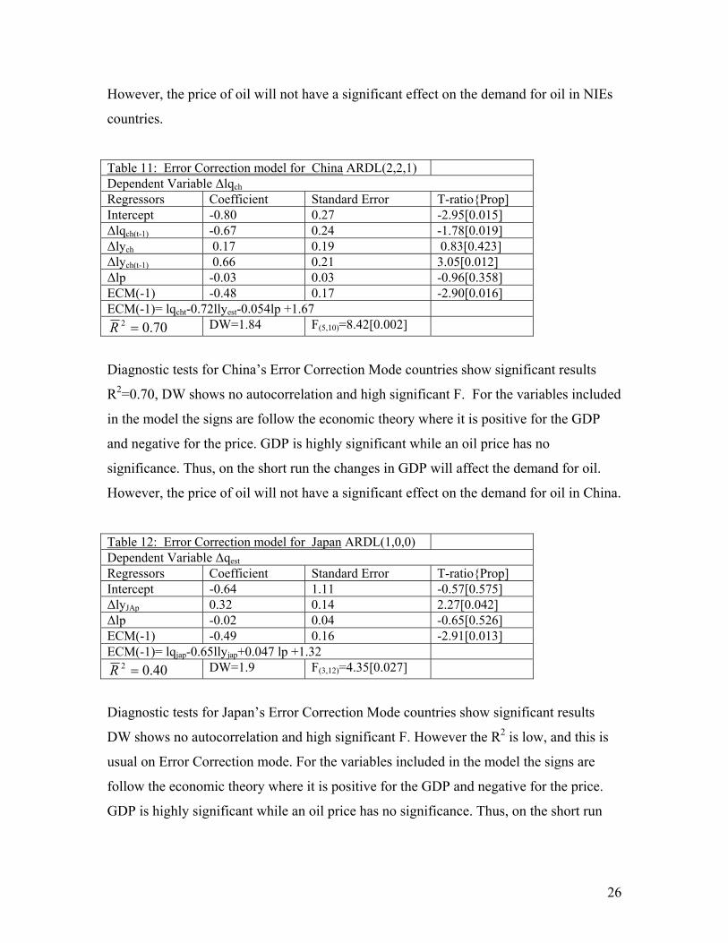
Table 11: Error Correction model for China ARDL(2,2,1) Dependent Variable ∆lqch Regressors Coefficient Standard Error T-ratio{Prop] Intercept -0.80 0.27 -2.95[0.015] ∆lqch(t-1) -0.67 0.24 -1.78[0.019] ∆lych 0.17 0.19 0.83[0.423] ∆lych(t-1) 0.66 0.21 3.05[0.012] ∆lp -0.03 0.03 -0.96[0.358] ECM(-1) -0.48 0.17 -2.90[0.016] ECM(-1)= lqcht-0.72llyest-0.054lp +1.67
70.02 =R DW=1.84 F(5,10)=8.42[0.002]
Diagnostic tests for China’s Error Correction Mode countries show significant results
R2=0.70, DW shows no autocorrelation and high significant F. For the variables included
in the model the signs are follow the economic theory where it is positive for the GDP
and negative for the price. GDP is highly significant while an oil price has no
significance. Thus, on the short run the changes in GDP will affect the demand for oil.
However, the price of oil will not have a significant effect on the demand for oil in China.
Table 12: Error Correction model for Japan ARDL(1,0,0) Dependent Variable ∆qest Regressors Coefficient Standard Error T-ratio{Prop] Intercept -0.64 1.11 -0.57[0.575] ∆lyJAp 0.32 0.14 2.27[0.042] ∆lp -0.02 0.04 -0.65[0.526] ECM(-1) -0.49 0.16 -2.91[0.013] ECM(-1)= lqjap-0.65llyjap+0.047 lp +1.32
40.02 =R DW=1.9 F(3,12)=4.35[0.027]
Diagnostic tests for Japan’s Error Correction Mode countries show significant results
DW shows no autocorrelation and high significant F. However the R2 is low, and this is
usual on Error Correction mode. For the variables included in the model the signs are
follow the economic theory where it is positive for the GDP and negative for the price.
GDP is highly significant while an oil price has no significance. Thus, on the short run
27
the changes in GDP will affect the demand for oil. However, the price of oil will not
have a significant effect on the demand for oil in Japan.
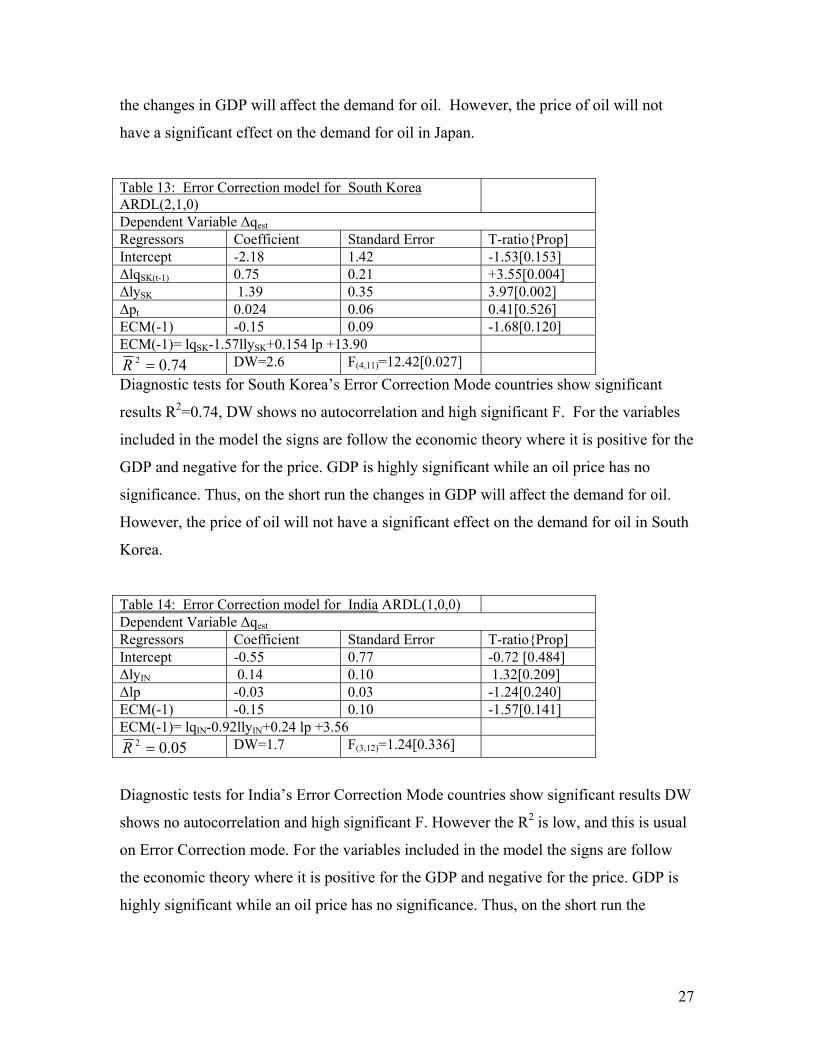
Table 13: Error Correction model for South Korea ARDL(2,1,0)
Dependent Variable ∆qest Regressors Coefficient Standard Error T-ratio{Prop] Intercept -2.18 1.42 -1.53[0.153] ∆lqSK(t-1) 0.75 0.21 +3.55[0.004] ∆lySK 1.39 0.35 3.97[0.002] ∆pt 0.024 0.06 0.41[0.526] ECM(-1) -0.15 0.09 -1.68[0.120] ECM(-1)= lqSK-1.57llySK+0.154 lp +13.90
74.02 =R DW=2.6 F(4,11)=12.42[0.027] Diagnostic tests for South Korea’s Error Correction Mode countries show significant
results R2=0.74, DW shows no autocorrelation and high significant F. For the variables
included in the model the signs are follow the economic theory where it is positive for the
GDP and negative for the price. GDP is highly significant while an oil price has no
significance. Thus, on the short run the changes in GDP will affect the demand for oil.
However, the price of oil will not have a significant effect on the demand for oil in South
Korea.
Table 14: Error Correction model for India ARDL(1,0,0) Dependent Variable ∆qest Regressors Coefficient Standard Error T-ratio{Prop] Intercept -0.55 0.77 -0.72 [0.484] ∆lyIN 0.14 0.10 1.32[0.209] ∆lp -0.03 0.03 -1.24[0.240] ECM(-1) -0.15 0.10 -1.57[0.141] ECM(-1)= lqIN-0.92llyIN+0.24 lp +3.56
05.02 =R DW=1.7 F(3,12)=1.24[0.336]
Diagnostic tests for India’s Error Correction Mode countries show significant results DW
shows no autocorrelation and high significant F. However the R2 is low, and this is usual
on Error Correction mode. For the variables included in the model the signs are follow
the economic theory where it is positive for the GDP and negative for the price. GDP is
highly significant while an oil price has no significance. Thus, on the short run the
28
changes in GDP will affect the demand for oil. However, the price of oil will not have a
significant effect on the demand for oil in India.
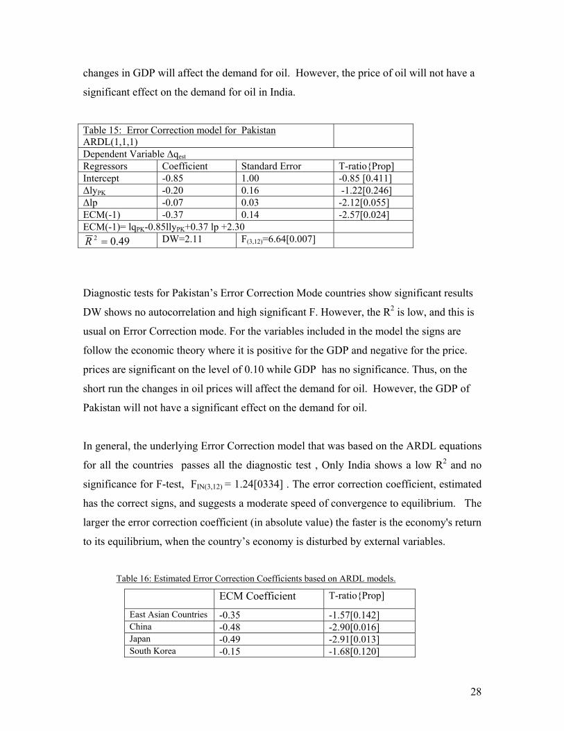
Table 15: Error Correction model for Pakistan ARDL(1,1,1)
Dependent Variable ∆qest Regressors Coefficient Standard Error T-ratio{Prop] Intercept -0.85 1.00 -0.85 [0.411] ∆lyPK -0.20 0.16 -1.22[0.246] ∆lp -0.07 0.03 -2.12[0.055] ECM(-1) -0.37 0.14 -2.57[0.024] ECM(-1)= lqPK-0.85llyPK+0.37 lp +2.30
49.02 =R DW=2.11 F(3,12)=6.64[0.007]
Diagnostic tests for Pakistan’s Error Correction Mode countries show significant results
DW shows no autocorrelation and high significant F. However, the R2 is low, and this is
usual on Error Correction mode. For the variables included in the model the signs are
follow the economic theory where it is positive for the GDP and negative for the price.
prices are significant on the level of 0.10 while GDP has no significance. Thus, on the
short run the changes in oil prices will affect the demand for oil. However, the GDP of
Pakistan will not have a significant effect on the demand for oil.
In general, the underlying Error Correction model that was based on the ARDL equations
for all the countries passes all the diagnostic test , Only India shows a low R2 and no
significance for F-test, FIN(3,12) = 1.24[0334] . The error correction coefficient, estimated
has the correct signs, and suggests a moderate speed of convergence to equilibrium. The
larger the error correction coefficient (in absolute value) the faster is the economy's return
to its equilibrium, when the country’s economy is disturbed by external variables.
Table 16: Estimated Error Correction Coefficients based on ARDL models.
ECM Coefficient T-ratio{Prop]
East Asian Countries -0.35 -1.57[0.142] China -0.48 -2.90[0.016] Japan -0.49 -2.91[0.013] South Korea -0.15 -1.68[0.120]
29
India -0.15 -1.57[0.141] Pakistan -0.37 -2.57[0.024]
The long run and short run elasticities were calculated from the ARDL models for all
different countries. It shows that the long-run elasticities were greater more than the
short-run
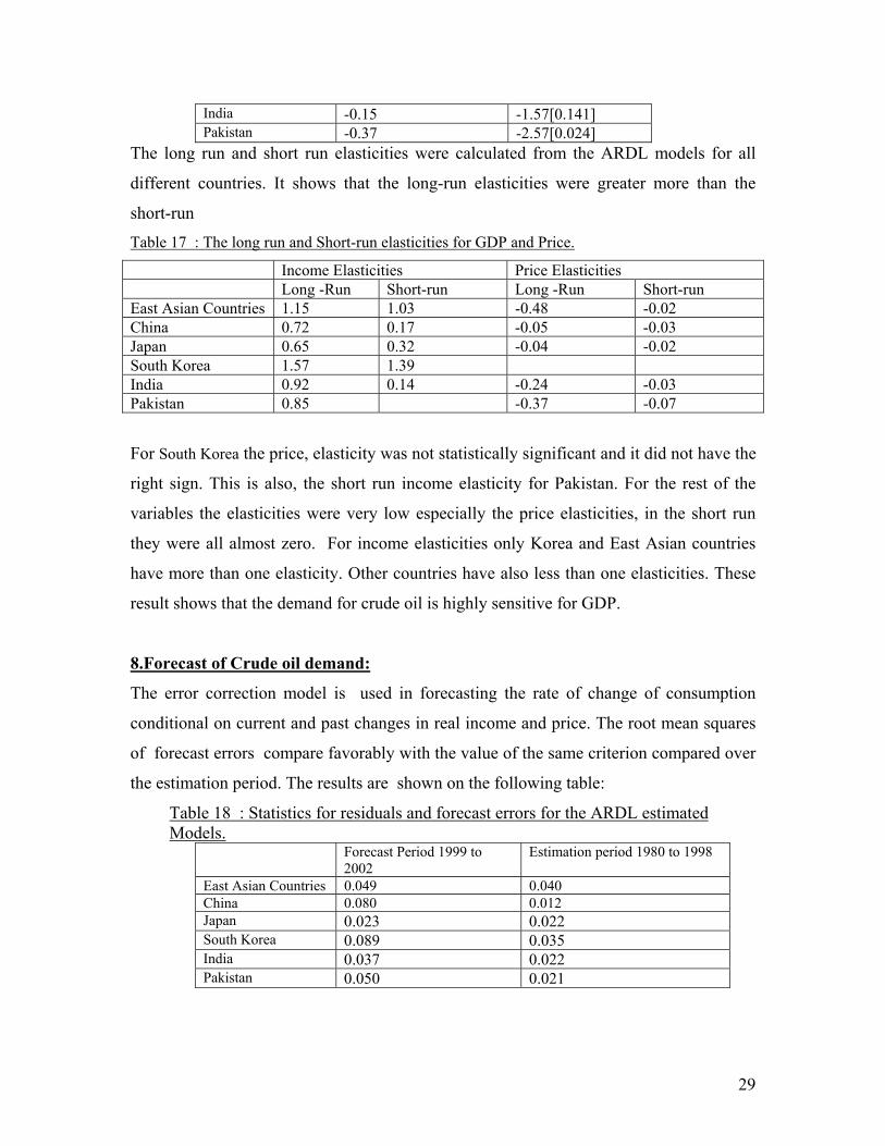
Table 17 : The long run and Short-run elasticities for GDP and Price.
Income Elasticities Price Elasticities Long -Run Short-run Long -Run Short-run East Asian Countries 1.15 1.03 -0.48 -0.02 China 0.72 0.17 -0.05 -0.03 Japan 0.65 0.32 -0.04 -0.02 South Korea 1.57 1.39 India 0.92 0.14 -0.24 -0.03 Pakistan 0.85 -0.37 -0.07
For South Korea the price, elasticity was not statistically significant and it did not have the
right sign. This is also, the short run income elasticity for Pakistan. For the rest of the
variables the elasticities were very low especially the price elasticities, in the short run
they were all almost zero. For income elasticities only Korea and East Asian countries
have more than one elasticity. Other countries have also less than one elasticities. These
result shows that the demand for crude oil is highly sensitive for GDP.
8.Forecast of Crude oil demand:
The error correction model is used in forecasting the rate of change of consumption
conditional on current and past changes in real income and price. The root mean squares
of forecast errors compare favorably with the value of the same criterion compared over
the estimation period. The results are shown on the following table:
Table 18 : Statistics for residuals and forecast errors for the ARDL estimated Models.
Forecast Period 1999 to 2002
Estimation period 1980 to 1998
East Asian Countries 0.049 0.040 China 0.080 0.012 Japan 0.023 0.022 South Korea 0.089 0.035 India 0.037 0.022 Pakistan 0.050 0.021
30
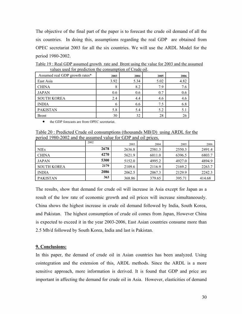
The objective of the final part of the paper is to forecast the crude oil demand of all the
six countries. In doing this, assumptions regarding the real GDP are obtained from
OPEC secretariat 2003 for all the six countries. We will use the ARDL Model for the
period 1980-2002.
Table 19 : Real GDP assumed growth rate and Brent using the value for 2003 and the assumed values used for prediction the consumption of Crude oil.
Assumed real GDP growth rates* 2003 2004 2005 2006
East Asia 3.92 5.34 5.02 4.82 CHINA 8 8.2 7.9 7.6 JAPAN 0.6 0.6 0.7 0.6 SOUTH KOREA 2.4 4.4 4.6 4.6 INDIA 6 6.6 7.5 6.8 PAKISTAN 5.8 5.4 5.2 5.1 Brent 30 32 28 26
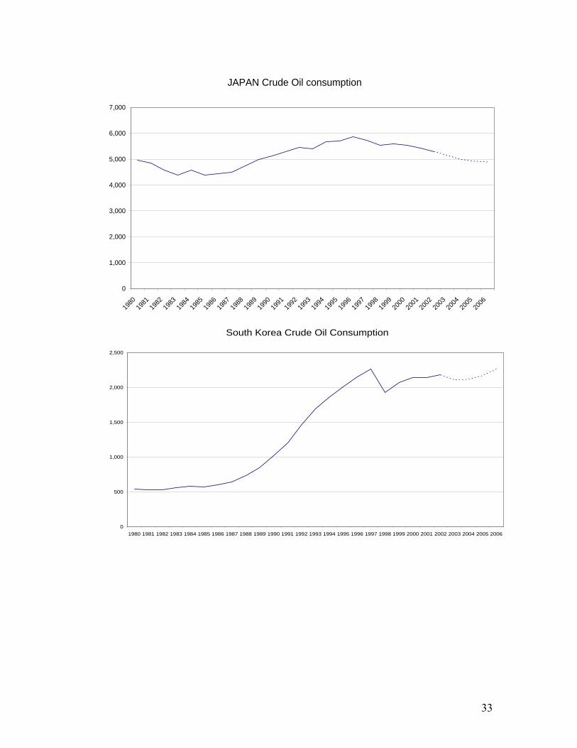
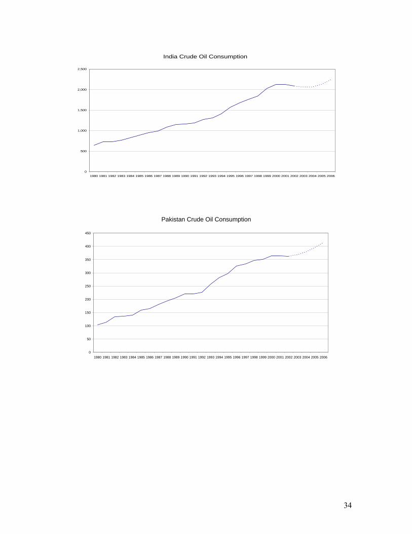
• the GDP forecasts are from OPEC secretariat. Table 20 : Predicted Crude oil consumptions (thousands MB/D) using ARDL for the period 1980-2002 and the assumed value for GDP and oil prices. 2002 2003 2004 2005 2006
NIEs 2678 2636.8 2581.3 2550.3 2491.4 CHINA 4270 5621.9 6011.0 6396.5 6803.7 JAPAN 5300 5152.0 4995.2 4927.0 4894.9 SOUTH KOREA 2179 2109.6 2116.9 2169.2 2263.7 INDIA 2086 2062.5 2067.3 2129.9 2242.3 PAKISTAN 363 368.86 379.65 395.71 414.68
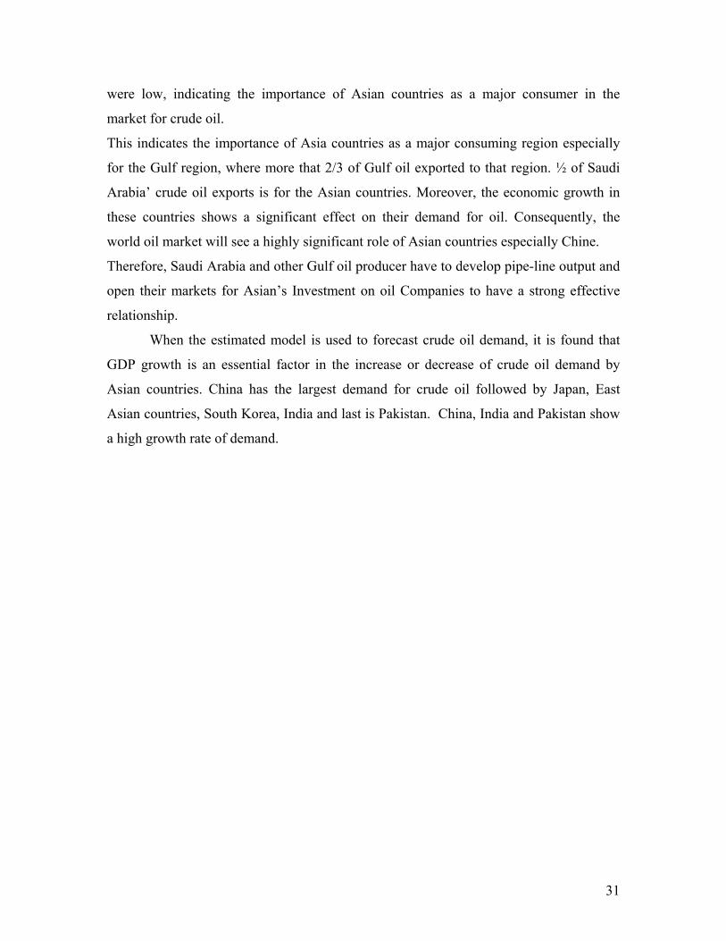
The results, show that demand for crude oil will increase in Asia except for Japan as a
result of the low rate of economic growth and oil prices will increase simultaneously.
China shows the highest increase in crude oil demand followed by India, South Korea,
and Pakistan. The highest consumption of crude oil comes from Japan, However China
is expected to exceed it in the year 2003-2006, East Asian countries consume more than
2.5 Mb/d followed by South Korea, India and last is Pakistan.
9. Conclusions:
In this paper, the demand of crude oil in Asian countries has been analyzed. Using
cointegration and the extension of this, ARDL methods. Since the ARDL is a more
sensitive approach, more information is derived. It is found that GDP and price are
important in affecting the demand for crude oil in Asia. However, elasticities of demand
31
were low, indicating the importance of Asian countries as a major consumer in the
market for crude oil.
This indicates the importance of Asia countries as a major consuming region especially
for the Gulf region, where more that 2/3 of Gulf oil exported to that region. ½ of Saudi
Arabia’ crude oil exports is for the Asian countries. Moreover, the economic growth in
these countries shows a significant effect on their demand for oil. Consequently, the
world oil market will see a highly significant role of Asian countries especially Chine.
Therefore, Saudi Arabia and other Gulf oil producer have to develop pipe-line output and
open their markets for Asian’s Investment on oil Companies to have a strong effective
relationship.
When the estimated model is used to forecast crude oil demand, it is found that
GDP growth is an essential factor in the increase or decrease of crude oil demand by
Asian countries. China has the largest demand for crude oil followed by Japan, East
Asian countries, South Korea, India and last is Pakistan. China, India and Pakistan show
a high growth rate of demand.
32
East Asian Coutries Crude Oil consumption and
0
500
1000
1500
2000
2500
3000
1980 1981 1982 1983 1984 1985 1986 1987 1988 1989 1990 1991 1992 1993 1994 1995 1996 1997 1998 1999 2000 2001 2002 2003 2004 2005 2006
CHINA Crude Oil consumption
0
1,000
2,000
3,000
4,000
5,000
6,000
7,000
8,000
1980
1982
1984
1986
1988
1990
1992
1994
1996
1998
2000
2002
2004
2006
33
JAPAN Crude Oil consumption
0
1,000
2,000
3,000
4,000
5,000
6,000
7,000
1980
1981
1982
1983
1984
1985
1986
1987
1988
1989
1990
1991
1992
1993
1994
1995
1996
1997
1998
1999
2000
2001
2002
2003
2004
2005
2006
South Korea Crude Oil Consumption
0
500
1,000
1,500
2,000
2,500
1980 1981 1982 1983 1984 1985 1986 1987 1988 1989 1990 1991 1992 1993 1994 1995 1996 1997 1998 1999 2000 2001 2002 2003 2004 2005 2006
34
India Crude Oil Consumption
0
500
1,000
1,500
2,000
2,500
1980 1981 1982 1983 1984 1985 1986 1987 1988 1989 1990 1991 1992 1993 1994 1995 1996 1997 1998 1999 2000 2001 2002 2003 2004 2005 2006
Pakistan Crude Oil Consumption
0
50
100
150
200
250
300
350
400
450
1980 1981 1982 1983 1984 1985 1986 1987 1988 1989 1990 1991 1992 1993 1994 1995 1996 1997 1998 1999 2000 2001 2002 2003 2004 2005 2006
35
REFERNCE Bentzen, J., and Engsted, T., (1993) " Short- and long-run elasticities in Energy Demand
a cointegration approach" Energy Economics. PP.(9-16) . Chan, H. and Lee, S. (1996) “Forecasting the Demand fro Energy in China” The Energy
Journal, Vol. 17, and No 1 PP (19-30). Dickey , D. A. and Fuller, W. A. (1981) Likelihood ratio statistics for
autoregressive time series with a unit root, Econometrica, 49, (1057-1071.) Dolado, J.J. and H. Lutkeopohl (1996), "Making Wald Test Work for Co integrated VAR
systems", Econometric Reviews, 15, pp (369-386.) Engle, R. and Granger, C. (1987)" Cointegration and error-correction: Representation
estimation and testing" Econometrica, Vol 55, pp (251-276.) Granger, C.(1988) " Some recent developments in a concept of Causality" Journal of
Econometrics, 39. pp (199-211). Granger, C.W.J. (1983) “Cointegration Variables and Error-Correction Models.”
UCDS Discussion Paper 86-13. Department of Economics, University of California-San Diego.
Hall, D. Anderson, H. M. Granger, C. W.J. (1994) A cointegration analysis of treasury
Bill yield, Review of Economics and Statistics, 74, 116-26. Han, X. and Lakshmanan, T., (1994) “Structural Changes and Energy Consumption in
the Japanese Economy 1975-85: An Input-Output Analysis. “ The Energy Journal, Vol, 15, No, 3.pp165-188.
Harvey, A. (1990), "The Econometric Analysis of Time Series" Second edi. LSE
Handbooks in Economics. Phillip Allan. London. Johansen, S. (1988), "Statistical Analysis of Cointegration Vectors", Journal of Economic
Dynamic and Control, 12, PP. 231-254. Johansen, S. (1991) . “Estimating and Hypothesis testing of Cointegration Vectors in
Gaussian Vector Autoregressive Models” Econometrica 59, 1551-1589. Johansen, S. and Jueslius, K. (1990) Maximum Likelihood Estimation And Inference On
Cointegration With Application To The Demand For Money, Oxford Bulletin of Economics and Statistics, 52, 169-209.

36
Masih, A. and Masih, R. (1996) " Energy consumption, real income and temporal causality: result from a multi-country based on counteraction and error-correction modeling" Energy Economics 18 PP 165-183.
Masih, A. and Masih, R. (1997) " On the temporal causal relationship between energy
consumption real income, and prices: some new evidence from Asian-energy dependent NICs Based on a multivariate cointegration/vector error-correction approach." Journal of Policy Modeling, Vol. 19, 4 PP 417-440.
McRae, R. (1994) “Gasoline Demand in Developing Asian Countries” Energy Journal,
Vol. 15, No 1. PP) 143-164). Asafu-Adjaye, J. (2000) "The relationship between energy consumption, energy prices
and economic growth: time series evidence from Asian developing countries" Energy Economics, Volume 22 Issue 6, Pages 615-625.
Pesaran , Shin and Smith.(2001), "Bound Testing Approaches to the Analysis of Level
Relationship. Journal of Applied Econometric Special Issue in Honor of J.D. Saragn on the theme "Studies in Empirical Macro econometric" Eds D.F. Hendry and M.H. Pesaran. Vol, 16. PP (289-326).
Pesaran, M., and Pesaran, B. (1997) " Working with Microfit 4.0 Interactive
Econometric Analysis" Oxford University Press Oxford. Peseran , M. and Shin, Y (1999) "An Autoregressive Distributed Lag Modeling
Approach to Cointegration Analysis" in (Ed) s storm, Econometric and Economic Theory in the 20th century: The ranger Frisch Centennial Symposium, Chapter 11. Cambridge University Press, Cambridge.
Salamah, M. (2003) “Quest for Middle East oil: the US verses the Asian-Pacific region.”
Energy Policy 31 PP (1085-1091)