DEMAND FORECASTING

The Context of Demand Forecasting

The Importance of Demand Forecasting

Forecasting product demand is crucial to any supplier, manufacturer, or retailer. Forecasts of future demand will determine the quantities that should be purchased, produced, and shipped. Demand forecasts are necessary since the basic operations process, moving from the suppliers' raw materials to finished goods in the customers' hands, takes time. Most firms cannot simply wait for demand to emerge and then react to it. Instead, they must anticipate and plan for future demand so that they can react immediately to customer orders as they occur. In other words, most manufacturers "make to stock" rather than "make to order" – they plan ahead and then deploy inventories of finished goods into field locations. Thus, once a customer order materializes, it can be fulfilled immediately – since most customers are not willing to wait the time it would take to actually process their order throughout the supply chain and make the product based on their order. An order cycle could take weeks or months to go back through part suppliers and sub-assemblers, through manufacture of the product, and through to the eventual shipment of the order to the customer.

Firms that offer rapid delivery to their customers will tend to force all competitors in the market to keep finished good inventories in order to provide fast order cycle times. As a result, virtually every organization involved needs to manufacture or at least order parts based on a forecast of future demand. The ability to accurately forecast demand also affords the firm opportunities to control costs through leveling its production quantities, rationalizing its transportation, and generally planning for efficient logistics operations.

In general practice, accurate demand forecasts lead to efficient operations and high levels of customer service, while inaccurate forecasts will inevitably lead to inefficient, high cost operations and/or poor levels of customer service. In many supply chains, the most important action we can take to improve the efficiency and effectiveness of the logistics process is to improve the quality of the demand forecasts.

Forecasting Demand in a Logistics System

Logistics professionals are typically interested in where and when customer demand will materialize. Consider a retailer selling through five superstores in Boston, New York, Detroit, Miami, and Chicago. It is not sufficient to know that the total demand will be 5,000 units per month, or, say, 1,000 units per month per store, on the average. Rather it is important to know, for example, how much the Boston store will sell in a specific month, since specific stores must be supplied with goods at specific times. The requirement might be to forecast the monthly demand for an item at the Boston superstore for the first three months of the next year. Using available historical data, without any further analysis, the best guess of monthly demand in the coming months would probably

1

be the average monthly sales over the last few years. The analytic challenge is to come up with a better forecast than this simple average.

Since the logistics system must satisfy specific demand, in other words what is needed, where and when, accurate forecasts must be generated at the Stock Keeping Unit (SKU) level, by stocking location, and by time period. Thus, the logistics information system must often generate thousands of individual forecasts each week. This suggests that useful forecasting procedures must be fairly "automatic"; that is, the forecasting method should operate without constant manual intervention or analyst input.

Forecasting is a problem that arises in many economic and managerial contexts, and hundreds of forecasting procedures have been developed over the years, for many different purposes, both in and outside of business enterprises. The procedures that we will discuss have proven to be very applicable to the task of forecasting product demand in a logistics system. Other techniques, which can be quite useful for other forecasting problems, have shown themselves to be inappropriate or inadequate to the task of demand forecasting in logistics systems. In many large firms, several organizations are involved in generating forecasts. The marketing department, for example, will generate high-level long-term forecasts of market demand and market share of product families for planning purposes. Marketing will also often develop short-term forecasts to help set sales targets or quotas. There is frequently strong organizational pressure on the logistics group to simply use these forecasts, rather than generating additional demand forecasts within the logistics system. After all, the logic seems to go, these marketing forecasts cost money to develop, and who is in a better position than marketing to assess future demand, and "shouldn’t we all be working with the same game plan anyway…?"

In practice, however, most firms have found that the planning and operation of an effective logistics system requires the use of accurate, disaggregated demand forecasts. The manufacturing organization may need a forecast of total product demand by week, and the marketing organization may need to know what the demand may be by region of the country and by quarter. The logistics organization needs to store specific SKUs in specific warehouses and to ship them on particular days to specific stores. Thus the logistics system, in contrast, must often generate weekly, or even daily, forecasts at the SKU level of detail for each of hundreds of individual stocking locations, and in most firms, these are generated nowhere else.

An important issue for all forecasts is the "horizon;" that is, how far into the future must the forecast project? As a general rule, the farther into the future we look, the more clouded our vision becomes -- long range forecasts will be less accurate that short range forecasts. The answer depends on what the forecast is used for. For planning new manufacturing facilities, for example, we may need to forecast demand many years into the future since the facility will serve the firm for many years. On the other hand, these forecasts can be fairly aggregate since they need not be SKU-specific or broken out by stockage location. For purposes of operating the logistics system, the forecasting horizon need be no longer than the cycle time for the product. For example, a given logistics system might be able to routinely purchase raw materials, ship them to manufacturing

2

locations, generate finished goods, and then ship the product to its field locations in, say, ninety days. In this case, forecasts of SKU - level customer demand which can reach ninety days into the future can tell us everything we need to know to direct and control the on-going logistics operation.

It is also important to note that the demand forecasts developed within the logistics system must be generally consistent with planning numbers generated by the production and marketing organizations. If the production department is planning to manufacture two million units, while the marketing department expects to sell four million units, and the logistics forecasts project a total demand of one million units, senior management must reconcile these very different visions of the future.

The Nature of Customer Demand

Most of the procedures in this chapter are intended to deal with the situation where the demand to be forecasted arises from the actions of the firm’s customer base. Customers are assumed to be able to order what, where, and when they desire. The firm may be able to influence the amount and timing of customer demand by altering the traditional "marketing mix" variables of product design, pricing, promotion, and distribution. On the other hand, customers remain free agents who react to a complex, competitive marketplace by ordering in ways that are often difficult to understand or predict. The firm’s lack of prior knowledge about how the customers will order is the heart of the forecasting problem – it makes the actual demand random.

However, in many other situations where inbound flows of raw materials and component parts must be predicted and controlled, these flows are not rooted in the individual decisions of many customers, but rather are based on a production schedule. Thus, if TDY Inc. decides to manufacture 1,000 units of a certain model of personal computer during the second week of October, the parts requirements for each unit are known. Given each part supplier’s lead-time requirements, the total parts requirement can be determined through a structured analysis of the product's design and manufacturing process. Forecasts of customer demand for the product are not relevant to this analysis. TDY, Inc., may or may not actually sell the 1,000 computers, but that is a different issue altogether. Once they have committed to produce 1,000 units, the inbound logistics system must work towards this production target. The Material Requirements Planning (MRP) technique is often used to handle this kind of demand. This demand for component parts is described as dependent demand (because it is dependent on the production requirement), as contrasted with independent demand, which would arise directly from customer orders or purchases of the finished goods. The MRP technique creates a deterministic demand schedule for component parts, which the material manager or the inbound logistics manager must meet. Typically a detailed MRP process is conducted only for the major components (in this case, motherboards, drives, keyboards, monitors, and so forth). The demand for other parts, such as connectors and memory chips, which are used in many different product lines, is often simply estimated and ordered by using statistical forecasting methods such as those described in this chapter.

3

General Approaches to Forecasting

All firms forecast demand, but it would be difficult to find any two firms that forecast demand in exactly the same way. Over the last few decades, many different forecasting techniques have been developed in a number of different application areas, including engineering and economics. Many such procedures have been applied to the practical problem of forecasting demand in a logistics system, with varying degrees of success. Most commercial software packages that support demand forecasting in a logistics system include dozens of different forecasting algorithms that the analyst can use to generate alternative demand forecasts. While scores of different forecasting techniques exist, almost any forecasting procedure can be broadly classified into one of the following four basic categories based on the fundamental approach towards the forecasting problem that is employed by the technique.

1. Judgmental Approaches. The essence of the judgmental approach is to address the forecasting issue by assuming that someone else knows and can tell you the right answer. That is, in a judgment-based technique we gather the knowledge and opinions of people who are in a position to know what demand will be. For example, we might conduct a survey of the customer base to estimate what our sales will be next month.

2. Experimental Approaches. Another approach to demand forecasting, which is appealing when an item is "new" and when there is no other information upon which to base a forecast, is to conduct a demand experiment on a small group of customers and to extrapolate the results to a larger population. For example, firms will often test a new consumer product in a geographically isolated "test market" to establish its probable market share. This experience is then extrapolated to the national market to plan the new product launch. Experimental approaches are very useful and necessary for new products, but for existing products that have an accumulated historical demand record it seems intuitive that demand forecasts should somehow be based on this demand experience. For most firms (with some very notable exceptions) the large majority of SKUs in the product line have long demand histories.

3. Relational/Causal Approaches. The assumption behind a causal or relational forecast is that, simply put, there is a reason why people buy our product. If we can understand what that reason (or set of reasons) is, we can use that understanding to develop a demand forecast. For example, if we sell umbrellas at a sidewalk stand, we would probably notice that daily demand is strongly correlated to the weather – we sell more umbrellas when it rains. Once we have established this relationship, a good weather forecast will help us order enough umbrellas to meet the expected demand.

4. "Time Series" Approaches. A time series procedure is fundamentally different than the first three approaches we have discussed. In a pure time series technique, no judgment or expertise or opinion is sought. We do not look for "causes" or relationships or factors which somehow "drive" demand. We do not test items or experiment with

4

customers. By their nature, time series procedures are applied to demand data that are longitudinal rather than cross-sectional. That is, the demand data represent experience that is repeated over time rather than across items or locations. The essence of the approach is to recognize (or assume) that demand occurs over time in patterns that repeat themselves, at least approximately. If we can describe these general patterns or tendencies, without regard to their "causes", we can use this description to form the basis of a forecast.

In one sense, all forecasting procedures involve the analysis of historical experience into patterns and the projection of those patterns into the future in the belief that the future will somehow resemble the past. The differences in the four approaches are in the way this "search for pattern" is conducted. Judgmental approaches rely on the subjective, ad-hoc analyses of external individuals. Experimental tools extrapolate results from small numbers of customers to large populations. Causal methods search for reasons for demand. Time series techniques simply analyze the demand data themselves to identify temporal patterns that emerge and persist.

Judgmental Approaches to Forecasting

By their nature, judgment-based forecasts use subjective and qualitative data to forecast future outcomes. They inherently rely on expert opinion, experience, judgment, intuition, conjecture, and other "soft" data. Such techniques are often used when historical data are not available, as is the case with the introduction of a new product or service, and in forecasting the impact of fundamental changes such as new technologies, environmental changes, cultural changes, legal changes, and so forth. Some of the more common procedures include the following:

Surveys. This is a "bottom up" approach where each individual contributes a piece of what will become the final forecast. For example, we might poll or sample our customer base to estimate demand for a coming period. Alternatively, we might gather estimates from our sales force as to how much each salesperson expects to sell in the next time period. The approach is at least plausible in the sense that we are asking people who are in a position to know something about future demand. On the other hand, in practice there have proven to be serious problems of bias associated with these tools. It can be difficult and expensive to gather data from customers. History also shows that surveys of "intention to purchase" will generally over-estimate actual demand – liking a product is one thing, but actually buying it is often quite another. Sales people may also intentionally (or even unintentionally) exaggerate or underestimate their sales forecasts based on what they believe their supervisors want them to say. If the sales force (or the customer base) believes that their forecasts will determine the level of finished goods inventory that will be available in the next period, they may be sorely tempted to inflate their demand estimates so as to insure good inventory availability. Even if these biases could be eliminated or controlled, another serious problem would probably remain. Sales people might be able to estimate their weekly dollar volume or total unit sales, but they are not likely to be able to develop credible estimates at the SKU level that the logistics system will require. For

5

these reasons it will seldom be the case that these tools will form the basis of a successful demand forecasting procedure in a logistics system.

Consensus methods. As an alternative to the "bottom-up" survey approaches, consensus methods use a small group of individuals to develop general forecasts. In a “Jury of Executive Opinion”, for example, a group of executives in the firm would meet and develop through debate and discussion a general forecast of demand. Each individual would presumably contribute insight and understanding based on their view of the market, the product, the competition, and so forth. Once again, while these executives are undoubtedly experienced, they are hardly disinterested observers, and the opportunity for biased inputs is obvious. A more formal consensus procedure, called “The Delphi Method”, has been developed to help control these problems. In this technique, a panel of disinterested technical experts is presented with a questionnaire regarding a forecast. The answers are collected, processed, and re-distributed to the panel, making sure that all information contributed by any panel member is available to all members, but on an anonymous basis. Each expert reflects on the gathering opinion. A second questionnaire is then distributed to the panel, and the process is repeated until a consensus forecast is reached. Consensus methods are usually appropriate only for highly aggregate and usually quite long-range forecasts. Once again, their ability to generate useful SKU level forecasts is questionable, and it is unlikely that this approach will be the basis for a successful demand forecasting procedure in a logistics system.

Judgment-based methods are important in that they are often used to determine an enterprise's strategy. They are also used in more mundane decisions, such as determining the quality of a potential vendor by asking for references, and there are many other reasonable applications. It is true that judgment based techniques are an inadequate basis for a demand forecasting system, but this should not be construed to mean that judgment has no role to play in logistics forecasting or that salespeople have no knowledge to bring to the problem. In fact, it is often the case that sales and marketing people have valuable information about sales promotions, new products, competitor activity, and so forth, which should be incorporated into the forecast somehow. Many organizations treat such data as additional information that is used to modify the existing forecast rather than as the baseline data used to create the forecast in the first place.

Experimental Approaches to Forecasting

In the early stages of new product development it is important to get some estimate of the level of potential demand for the product. A variety of market research techniques are used to this end.

Customer Surveys are sometimes conducted over the telephone or on street corners, at shopping malls, and so forth. The new product is displayed or described, and potential customers are asked whether they would be interested in purchasing the item. While this approach can help to isolate attractive or unattractive product features, experience has shown that "intent to purchase" as measured in this way is difficult to

6

translate into a meaningful demand forecast. This falls short of being a true “demand experiment”.

Consumer Panels are also used in the early phases of product development. Here a small group of potential customers are brought together in a room where they can use the product and discuss it among themselves. Panel members are often paid a nominal amount for their participation. Like surveys, these procedures are more useful for analyzing product attributes than for estimating demand, and they do not constitute true “demand experiments” because no purchases take place.

Test Marketing is often employed after new product development but prior to a full-scale national launch of a new brand or product. The idea is to choose a relatively small, reasonably isolated, yet somehow demographically "typical" market area. In the United States, this is often a medium sized city such as Cincinnati or Buffalo. The total marketing plan for the item, including advertising, promotions, and distribution tactics, is "rolled out" and implemented in the test market, and measurements of product awareness, market penetration, and market share are made. While these data are used to estimate potential sales to a larger national market, the emphasis here is usually on "fine-tuning" the total marketing plan and insuring that no problems or potential embarrassments have been overlooked. For example, Proctor and Gamble extensively test-marketed its Pringles potato chip product made with the fat substitute Olestra to assure that the product would be broadly acceptable to the market.

Scanner Panel Data procedures have recently been developed that permit demand experimentation on existing brands and products. In these procedures, a large set of household customers agrees to participate in an ongoing study of their grocery buying habits. Panel members agree to submit information about the number of individuals in the household, their ages, household income, and so forth. Whenever they buy groceries at a supermarket participating in the research, their household identity is captured along with the identity and price of every item they purchased. This is straightforward due to the use of UPC codes and optical scanners at checkout. This procedure results in a rich database of observed customer buying behavior. The analyst is in a position to see each purchase in light of the full set of alternatives to the chosen brand that were available in the store at the time of purchase, including all other brands, prices, sizes, discounts, deals, coupon offers, and so on. Statistical models such as discrete choice models can be used to analyze the relationships in the data. The manufacturer and merchandiser are now in a position to test a price promotion and estimate its probable effect on brand loyalty and brand switching behavior among customers in general. This approach can develop valuable insight into demand behavior at the customer level, but once again it can be difficult to extend this insight directly into demand forecasts in the logistics system.

Relational/Causal Approaches to Forecasting

Suppose our firm operates retail stores in a dozen major cities, and we now decide to open a new store in a city where we have not operated before. We will need to forecast

7

what the sales at the new store are likely to be. To do this, we could collect historical sales data from all of our existing stores. For each of these stores we could also collect relevant data related to the city's population, average income, the number of competing stores in the area, and other presumably relevant data. These additional data are all referred to as explanatory variables or independent variables in the analysis. The sales data for the stores are considered to be the dependent variable that we are trying to explain or predict.

The basic premise is that if we can find relationships between the explanatory variables (population, income, and so forth) and sales for the existing stores, then these relationships will hold in the new city as well. Thus, by collecting data on the explanatory variables in the target city and applying these relationships, sales in the new store can be estimated. In some sense the posture here is that the explanatory variables "cause" the sales. Mathematical and statistical procedures are used to develop and test these explanatory relationships and to generate forecasts from them. Causal methods include the following:

Econometric models, such as discrete choice models and multiple regression. More elaborate systems involving sets of simultaneous regression equations can also be attempted. These advanced models are beyond the scope of this book and are not generally applicable to the task of forecasting demand in a logistics system.

Input-output models estimate the flow of goods between markets and industries. These models ensure the integrity of the flows into and out of the modeled markets and industries; they are used mainly in large-scale macro-economic analysis and were not found useful in logistics applications.

Life cycle models look at the various stages in a product's "life" as it is launched, matures, and phases out. These techniques examine the nature of the consumers who buy the product at various stages ("early adopters," "mainstream buyers," "laggards," etc.) to help determine product life cycle trends in the demand pattern. Such models are used extensively in industries such as high technology, fashion, and some consumer goods facing short product life cycles. This class of model is not distinct from the others mentioned here as the characteristics of the product life cycle can be estimated using, for example, econometric models. They are mentioned here as a distinct class because the overriding "cause" of demand with these models is assumed to be the life cycle stage the product is in.

Simulation models are used to model the flows of components into manufacturing plants based on MRP schedules and the flow of finished goods throughout distribution networks to meet customer demand. There is little theory to building such simulation models. Their strength lies in their ability to account for many time lag effects and complicated dependent demand schedules. They are, however, typically cumbersome and complicated.

8

Time Series Approaches to Forecasting

Although all four approaches are sometimes used to forecast demand, generally the time-series approach is the most appropriate and the most accurate approach to generate the large number of short-term, SKU level, locally dis-aggregated forecasts required to operate a physical distribution system over a reasonably short time horizon. On the other hand, these time series techniques may not prove to be very accurate. If the firm has knowledge or insight about future events, such as sales promotions, which can be expected to dramatically alter the otherwise expected demand, some incorporation of this knowledge into the forecast through judgmental or relational means is also appropriate.

Many different time series forecasting procedures have been developed. These techniques include very simple procedures such as the Moving Average and various procedures based on the related concept of Exponential Smoothing. These procedures are extensively used in logistics systems, and they will be thoroughly discussed in this chapter. Other more complex procedures, such as the Box-Jenkins (ARIMA) Models, are also available and are sometimes used in logistics systems. However, in most cases these more sophisticated tools have not proven to be superior to the simpler tools, and so they are not widely used in logistics systems. Our treatment of them here will therefore be brief.

Basic Time Series Concepts

Before we begin our discussion of specific time series techniques, we will outline some concepts, definitions, and notation that will be common to all of the procedures.

Definitions and Notation

A time series is a set of observations of a process, taken at regular intervals. For example, the weekly demand for product number "XYZ" (a pair of 6 " bi-directional black speakers) at the St. Louis warehouse of the "Speakers-R-Us" Company during calendar year 1998 would be a time series with 52 observations, or data points. Note that this statement inherently involves aggregation over time, in that we do not keep a record of when during the week any single speaker was actually demanded. If this were in fact important, we could work with a daily time series with 365 observations per year. In practice, for purposes of operating logistics systems, most firms aggregate demand into weekly, bi-weekly, or monthly intervals.

We will use the notation Zt to represent observed demand at time t. Thus the statement "Z13 = 328" means that actual demand for an item in period 13 was 328 units. The notation Z't will designate a forecast, so that "Z'13 = 347" means that a forecast for demand in period 13 was 347 units. By convention, throughout this chapter we will consider that time "t" is "now"; all observations of demand up through and including time "t" are known, and the focus will be on developing a "one-period ahead" forecast, that is,

9

Z’t+1. Note that in the time series framework, such a forecast must be generated as a function of Zt-1, Zt-2, Zt-3, …-- the observed demand.

We intend for the forecasts to be accurate, but we do not expect them to be perfect or error-free. To measure the forecast accuracy, we define the error associated with any forecast to be et, where:

e Z Z ' t = -t t

That is, the error is the signed algebraic difference between the actual demand and the forecasted demand. A positive error indicates that the forecast was too low, and a negative error indicates an "over-forecast".

In the time series approach, we assume that the data at hand consist of some "pattern", which is consistent, and some noise, which is a non-patterned, random component that simply cannot be forecasted. Conceptually, we can think of noise as the way we recognize that a part of customers’ behavior is inherently random. Alternatively, we can think of a random noise term as simply a parsimonious way of representing the vast number of factors and influences which might effect demand in any given period (advertising, weather, traffic, competitors, and so forth) which we could never completely recognize and analyze in advance. The time series procedure attempts to capture and model the “pattern” and to ignore the “noise”. In statistical terms, we can model the noise component of the observation, nt, as a realization of a random variable, drawn from an arbitrary, time-invariant probability distribution with a mean of zero and a constant variance. We further assume that the realizations of the noise component are serially uncorrelated, so that no number of consecutive observations of the noise would provide any additional information about the next value in the series.

Time Series Patterns

The simplest time series would be stationary data. A series is said to be stationary if it maintains a persistent level over time, and if fluctuations around that level are merely random, that is, attributable only to noise. We can represent a stationary time series mathematically as a set of observations arising from a hypothetical generating process function of the form:

Z L et= +t

where L is some constant (the "level" of the series) and nt is the noise term associated with period t. This is a very simple process that is trivial to forecast – our forecast should always be:

'Z t +1 = L

It does not follow, however, that our forecasts will be particularly accurate. To the extent that the noise terms are small in absolute value, in comparison to the level term

10

(which is to say, to the extent that the variance of the probability distribution function from which the noise observations are drawn is small), the forecasts should be accurate. To the extent that the noise terms are relatively large, the series will be very volatile and the forecasts will suffer from large errors.

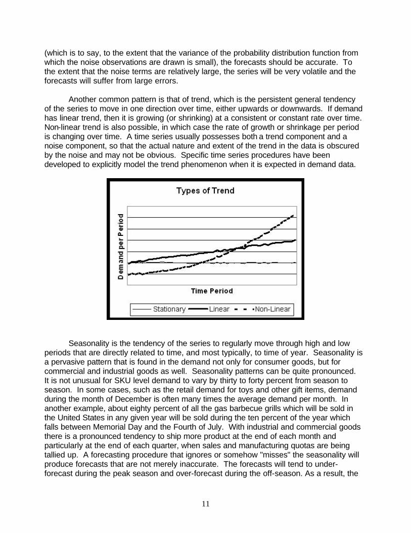
Another common pattern is that of trend, which is the persistent general tendency of the series to move in one direction over time, either upwards or downwards. If demand has linear trend, then it is growing (or shrinking) at a consistent or constant rate over time. Non-linear trend is also possible, in which case the rate of growth or shrinkage per period is changing over time. A time series usually possesses both a trend component and a noise component, so that the actual nature and extent of the trend in the data is obscured by the noise and may not be obvious. Specific time series procedures have been developed to explicitly model the trend phenomenon when it is expected in demand data.

Seasonality is the tendency of the series to regularly move through high and low periods that are directly related to time, and most typically, to time of year. Seasonality is a pervasive pattern that is found in the demand not only for consumer goods, but for commercial and industrial goods as well. Seasonality patterns can be quite pronounced. It is not unusual for SKU level demand to vary by thirty to forty percent from season to season. In some cases, such as the retail demand for toys and other gift items, demand during the month of December is often many times the average demand per month. In another example, about eighty percent of all the gas barbecue grills which will be sold in the United States in any given year will be sold during the ten percent of the year which falls between Memorial Day and the Fourth of July. With industrial and commercial goods there is a pronounced tendency to ship more product at the end of each month and particularly at the end of each quarter, when sales and manufacturing quotas are being tallied up. A forecasting procedure that ignores or somehow "misses" the seasonality will produce forecasts that are not merely inaccurate. The forecasts will tend to under-forecast during the peak season and over-forecast during the off-season. As a result, the

11

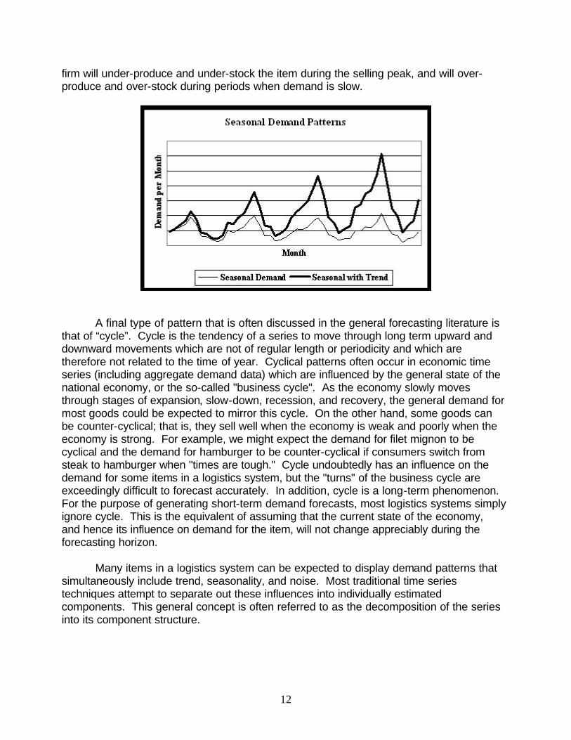
firm will under-produce and under-stock the item during the selling peak, and will over­produce and over-stock during periods when demand is slow.

A final type of pattern that is often discussed in the general forecasting literature is that of “cycle”. Cycle is the tendency of a series to move through long term upward and downward movements which are not of regular length or periodicity and which are therefore not related to the time of year. Cyclical patterns often occur in economic time series (including aggregate demand data) which are influenced by the general state of the national economy, or the so-called "business cycle". As the economy slowly moves through stages of expansion, slow-down, recession, and recovery, the general demand for most goods could be expected to mirror this cycle. On the other hand, some goods can be counter-cyclical; that is, they sell well when the economy is weak and poorly when the economy is strong. For example, we might expect the demand for filet mignon to be cyclical and the demand for hamburger to be counter-cyclical if consumers switch from steak to hamburger when "times are tough." Cycle undoubtedly has an influence on the demand for some items in a logistics system, but the "turns" of the business cycle are exceedingly difficult to forecast accurately. In addition, cycle is a long-term phenomenon. For the purpose of generating short-term demand forecasts, most logistics systems simply ignore cycle. This is the equivalent of assuming that the current state of the economy, and hence its influence on demand for the item, will not change appreciably during the forecasting horizon.

Many items in a logistics system can be expected to display demand patterns that simultaneously include trend, seasonality, and noise. Most traditional time series techniques attempt to separate out these influences into individually estimated components. This general concept is often referred to as the decomposition of the series into its component structure.

12

Accuracy and Bias

In general, a set of forecasts will be considered to be accurate if the forecast errors, that is, the set of et values which results from the forecasts, are sufficiently small. The next section presents statistics based on the forecast errors, which can be used to measure forecast accuracy. In thinking about forecast accuracy, it is important to bear in mind the distinction between error and noise. While related, they are not the same thing. Noise in the demand data is real and is uncontrollable and will cause error in the forecasts, because by our definition we cannot forecast the noise. On the other hand, we create the errors that we observe because we create the forecasts; better forecasts will have smaller errors.

In some cases demand forecasts are not merely inaccurate, but they also exhibit bias. Bias is the persistent tendency of the forecast to err in the same direction, that is, to consistently over-predict or under-predict demand. We generally seek forecasts which are as accurate and as unbiased as possible. Bias represents a pattern in the errors, suggesting that we have not found and exploited all of the pattern in the demand data. This in turn would suggest that the forecasting procedure being used is inappropriate. For example, suppose our forecasting system always gave us a forecast that was on average ten units below the actual demand for that period. If we always adjusted this forecast by adding ten units to it (thus correcting for the bias), the forecasts would become more accurate as well as more unbiased.

Logistics managers sometimes prefer to work with intentionally biased demand forecasts. In a situation where high levels of service are very important, some managers like to use forecasts that are "biased high" because they tend to build inventories and therefore reduce the incidence of stockouts. In a situation where there are severe penalties for holding too much inventory, managers sometimes prefer a forecast which is "biased low," because they would prefer to run the increased risk of stocking out rather than risk holding “excess” inventories. In some cases managers have even been known to manually adjust the system forecasts to create these biases in an attempt to drive the inventory in the desired direction. This is an extremely bad idea. The problem here is that there is no sound way to know how much to "adjust" the forecasts, since this depends in a fairly complicated way on the costs of inventory versus the costs of shortages. Neither of these costs is represented in any way in the forecasting data. The more sound approach is therefore to generate the most accurate and unbiased forecasts possible, and then to use these forecasts as planning inputs to inventory control algorithms that will explicitly consider the forecasting errors, inventory costs, and shortage costs, and that will then consciously trade-off all the relevant costs in arriving at a cost-effective inventory policy. If we attempt to inf luence the inventory by "adjusting" the forecasts up-front, we short-circuit this process without proper information.

13

Error Statistics

Given a set of n observations of the series Zt , and the corresponding forecasts Z't , we can define statistics based on the set of the error terms ( where et = Zt - Z't ) that are useful to describe and summarize the accuracy of the forecasts. These statistics are simple averages of some function of the forecast errors. While we are developing these statistics in the context of time-series forecasting, these measures are completely general. They can be applied to any set of forecast errors, no matter what technique had been used to generate the forecasts.

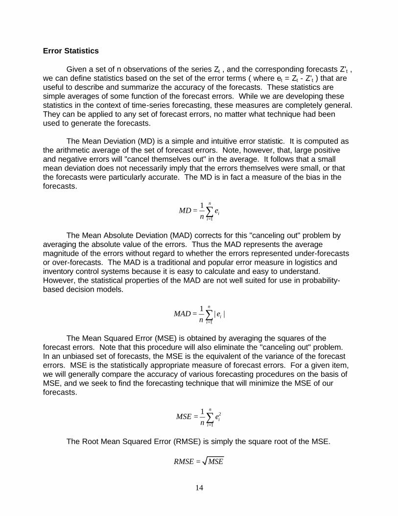
The Mean Deviation (MD) is a simple and intuitive error statistic. It is computed as the arithmetic average of the set of forecast errors. Note, however, that, large positive and negative errors will "cancel themselves out" in the average. It follows that a small mean deviation does not necessarily imply that the errors themselves were small, or that the forecasts were particularly accurate. The MD is in fact a measure of the bias in the forecasts.

n1

n MD = � ei

i=1

The Mean Absolute Deviation (MAD) corrects for this "canceling out" problem by averaging the absolute value of the errors. Thus the MAD represents the average magnitude of the errors without regard to whether the errors represented under-forecasts or over-forecasts. The MAD is a traditional and popular error measure in logistics and inventory control systems because it is easy to calculate and easy to understand. However, the statistical properties of the MAD are not well suited for use in probability-based decision models.

n1MAD = � | |

n ei

i=1

The Mean Squared Error (MSE) is obtained by averaging the squares of the forecast errors. Note that this procedure will also eliminate the "canceling out" problem. In an unbiased set of forecasts, the MSE is the equivalent of the variance of the forecast errors. MSE is the statistically appropriate measure of forecast errors. For a given item, we will generally compare the accuracy of various forecasting procedures on the basis of MSE, and we seek to find the forecasting technique that will minimize the MSE of our forecasts.

n1 2

n MSE = � ei

i=1

The Root Mean Squared Error (RMSE) is simply the square root of the MSE.

RMSE = MSE

14

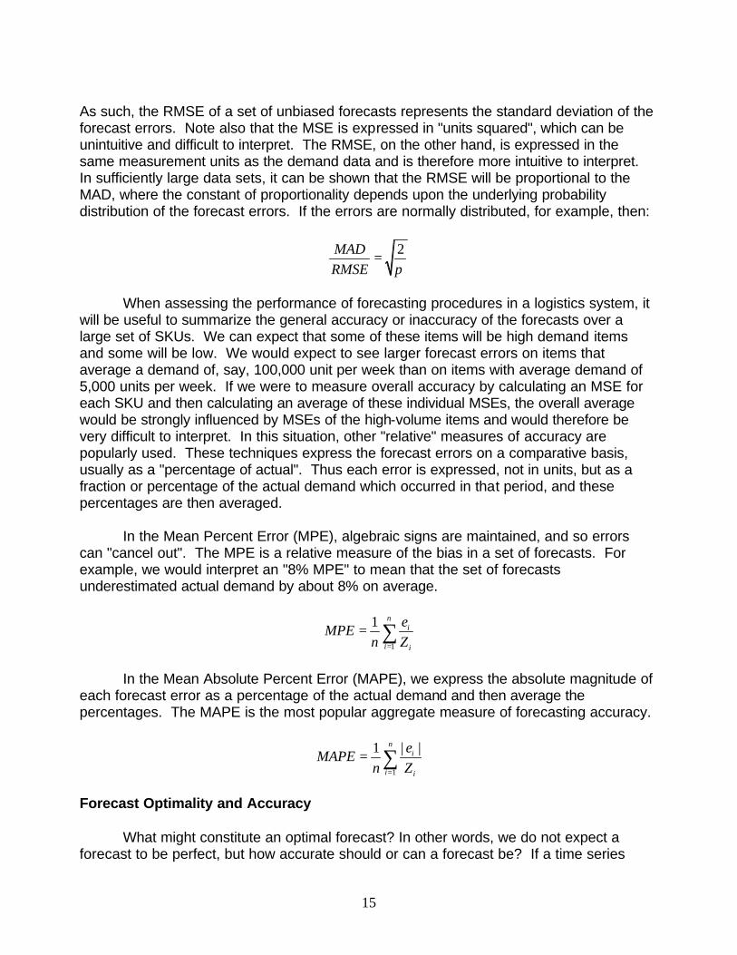
As such, the RMSE of a set of unbiased forecasts represents the standard deviation of the forecast errors. Note also that the MSE is expressed in "units squared", which can be unintuitive and difficult to interpret. The RMSE, on the other hand, is expressed in the same measurement units as the demand data and is therefore more intuitive to interpret. In sufficiently large data sets, it can be shown that the RMSE will be proportional to the MAD, where the constant of proportionality depends upon the underlying probability distribution of the forecast errors. If the errors are normally distributed, for example, then:

MAD 2 =

RMSE p

When assessing the performance of forecasting procedures in a logistics system, it will be useful to summarize the general accuracy or inaccuracy of the forecasts over a large set of SKUs. We can expect that some of these items will be high demand items and some will be low. We would expect to see larger forecast errors on items that average a demand of, say, 100,000 unit per week than on items with average demand of 5,000 units per week. If we were to measure overall accuracy by calculating an MSE for each SKU and then calculating an average of these individual MSEs, the overall average would be strongly influenced by MSEs of the high-volume items and would therefore be very difficult to interpret. In this situation, other "relative" measures of accuracy are popularly used. These techniques express the forecast errors on a comparative basis, usually as a "percentage of actual". Thus each error is expressed, not in units, but as a fraction or percentage of the actual demand which occurred in that period, and these percentages are then averaged.

In the Mean Percent Error (MPE), algebraic signs are maintained, and so errors can "cancel out". The MPE is a relative measure of the bias in a set of forecasts. For example, we would interpret an "8% MPE" to mean that the set of forecasts underestimated actual demand by about 8% on average.

n

n MPE = 1 � ei

i =1 Zi

In the Mean Absolute Percent Error (MAPE), we express the absolute magnitude of each forecast error as a percentage of the actual demand and then average the percentages. The MAPE is the most popular aggregate measure of forecasting accuracy.

� ei

n MAPE = 1 n | |

i =1 Zi

Forecast Optimality and Accuracy

What might constitute an optimal forecast? In other words, we do not expect a forecast to be perfect, but how accurate should or can a forecast be? If a time series

15

consists of pattern and noise, and if we understand the pattern perfectly, then in the long run our forecasts will only be wrong by the amount of the noise. In such a case, the MSE of the error terms would equal the variance of the noise terms. This situation would result in the lowest possible long-term MSE, and this situation would constitute an optimal forecast. No other set of forecasts could be more accurate in the long run unless they were somehow able to forecast the noise successfully, which by definition cannot be done. In practice, it is usually impossible to tell if a given set of forecasts is optimal because neither the generating process nor the distribution of the noise terms is known. The more relevant issue is whether we can find a set of forecasts that are better (more accurate) than the ones we are currently using.

How much accuracy can we expect or demand from our forecasting systems? This is a very difficult question to answer. Forecasting item level demand in a logistics system can be challenging, and the degree of success will vary from setting to setting based on the underlying volatility (or noise) in the demand processes. Having said that, many practitioners suggest that for short-term forecasts of SKU level demand for high volume items at the distribution center level, system-wide MAPE figures in the range of 10% to 15% would be considered very good. Many firms report MAPE performance in the range of 20%, 30%, or even higher. As we shall see, highly inaccurate forecasts will increase the need for safety stock in the inventory system and will reduce the customer service level. Thus the costs of inaccurate forecasting can be very high, and it is worth considerable effort to insure that demand forecasts are as accurate as we can make them.

Simple Time Series Methods

In this section we will develop and review some of the most popular time series techniques that have been applied to forecasting demand in logistics systems. All of these procedures are easy to implement in computer software and are widely available in commercial forecasting packages.

The Cumulative Mean

Consider the situation where demand is somehow known to be arising from a stationary generating process of the form:

Z L nt= +t

where the value of L (the “level” of the series) and the variance of the noise term are unknown. In the long run, the optimal forecast for this time series would be:

'Z t+1 = L

since we cannot forecast the noise. Unfortunately, we do not know L. Another way to think about this is to consider the expected value of any future observation at time t, where E[x] is the expected value of the random variable x:

16

t ] = t ] = L E[n L 0E[Z E[ L + n E[ ] + ] = + = Lt

This is so because L is a constant and the mean of the noise term is zero. It follows that the problem at hand is to develop the best possible estimate of L from the available data. Basic sampling logic would suggest that, since the underlying process never changes, we should use as large a sample as possible to sharpen our estimate of L. This would lead us to use a cumulative mean for the forecast. If we have data reaching back to period one, then at any subsequent period t:

t

t 'Z t+1 =

1 �Z i=1

i

We would simply let the forecast equal the average of all prior observations. As our demand experience grew, we would incorporate all of it into our estimate of L. As time passed, our forecasts would stabilize and converge towards L, because in the long run the noise terms will cancel each other out because their mean is zero. The more data we include in the average, the greater will be the tendency of the noise terms to sum to zero, thus revealing the true value of L.

Should this procedure be used to forecast demand in a logistics system? Given the demand generating process we have assumed, this technique is ideal. In the long run, it will generate completely unbiased forecasts. The accuracy of the forecasts will depend only upon the volatility of demand; that is, if the noise terms are large the forecasts will not be particularly accurate. On the other hand, without regard to how accurate the forecasts may be, they will be optimal. No other procedure can do a better job on this kind of data than the cumulative mean.

The issue of the utility of this tool, however, must be resolved on other grounds. If we have purely stationary demand data, there is no doubt that this is the technique of choice. On the other hand, very few items in a logistics system can be expected to show the extreme stability and simplicity of demand pattern implied by this generating process. Sometimes analysts are tempted to average together demand data going back five years or more because the data are available, because the data are "true" or accurate, and because "big samples are better." The issue here is not whether the historical demand truly happened -- the question is whether the very old data are truly representative of the current state of the demand process. To the extent that old data are no longer representative, their use will degrade the accuracy of the forecast, not improve it. This procedure will seldom be appropriate in a logistics system.

The Naive Forecast

Consider the situation where demand is arising according to the following generating process:

Z Z nt = +t t-1

17

Each observation of the process is simply the prior observation plus a random noise term, where the noise process has a mean of zero and a constant variance. This demand process is a "random walk". As a time series it is non-stationary and has virtually no pattern -- no level, trend, or seasonality. Such a series will simply wander through long upward and downward excursions. If we think in terms of the expected value of the next observation at any specific time t, we see that:

t ] = + t ] = t ] = 0E[Z E[ Z n E[ Zt -1] + E[n Z t -1 + = Zt -1t -1

because at time t , the value of Zt-1 is known and constant. This suggests that the best way to forecast this series would be:

'Z t+1 = Zt

Each forecast is simply the most recent prior observation. This approach is called a “naïve” forecast and is sometimes referred to as "Last is Next". This is, in fact, an almost instinctive way to forecast, and it is frequently used to generate simple short-term forecasts. It can be shown that, for this specific generating process, the naive forecast is unbiased and optimal. Accuracy will once again depend on the magnitude of the noise variance, but no other technique will do better in the long run.

It does not follow that this is a particularly useful tool in a logistics system. The naive forecast should only be used if demand truly behaves according to a random walk process. This will seldom be the case. Customers can be inscrutable at times, but aggregate demand for most items usually displays some discernable form or pattern. Using a naive forecast ignores this pattern, and potential accuracy is lost as a result.

As an illustration of how forecast errors can be inflated by using an inappropriate tool, look at what happens, for example, when we use a naive forecast on demand data from a simple, stationary demand process. If demand is being generated according to:

Z L n t= +t

where L is a constant and the noise terms have a mean of zero and a variance of s2, we have seen that the optimal forecasting procedure would be the cumulative mean, and that in the long run the accuracy of the forecasts would approach:

2MSE[Cumulative Mean] @ s

What would happen to the MSE if we used a naive forecast instead of the cumulative mean on this kind of data? In general, each error term would now be the difference between two serial observations:

t = ( - -e Z Z ' t ) = (Z Z t -1)t t

18

The expected value of the error terms would be:

t ] = - t ] - L LE[e E[Z Z t -1] = E[ L + n E[ L + n ] = - = 0t t -1

and so the resulting forecasts would be unbiased. However, the variance of the error terms would be:

t ]2V[e V[Z Z ] = V[L + + + t -1] 2st ] = - n V[ L n = t t -1

since L is a constant. It follows that the MSE of the naive forecasts will be twice as high as the MSE of the cumulative mean forecasts would have been on such a data set.

The Simple Moving Average

Sometimes the demand for an item in a logistics system may be essentially “flat” for a long period but then undergo a sudden shift or permanent change in level. This may occur, for example, because of a price change, the rise or fall of a competitor, or the redefinition of the customer support territory assigned to the inventory location. The shift may be due to the deliberate action of the firm, or it may occur without the firm's knowledge. That is, the time of occurrence and size of the shift may be essentially random from the firm's point of view. What forecasting procedure should be used on such an item? Prior to the change in level, a cumulative mean would work well. Once the shift has occurred, however, the cumulative mean will be persistently inaccurate because most of the data being averaged into the forecast is no longer representative of the new, changed level of the demand process. If a naive forecast is used, the forecast will react quickly to the change in level whenever it does occur, but it will also react to every single noise term as though it were a meaningful, permanent change in level as well, thus greatly increasing the forecast errors. A moving average represents a kind of compromise between these two extremes.

In a moving average, the forecast would be calculated as the average of the last “few” observations. If we let M equal the number of observations to be included in the moving average, then:

1 t

M 'Z t+1 = � Zi

i t M= + -1

For example, if we let M=3, we have a "three period moving average", and so, for example, at t = 7:

+ + 7 6Z '8 = Z Z Z 5

3

19

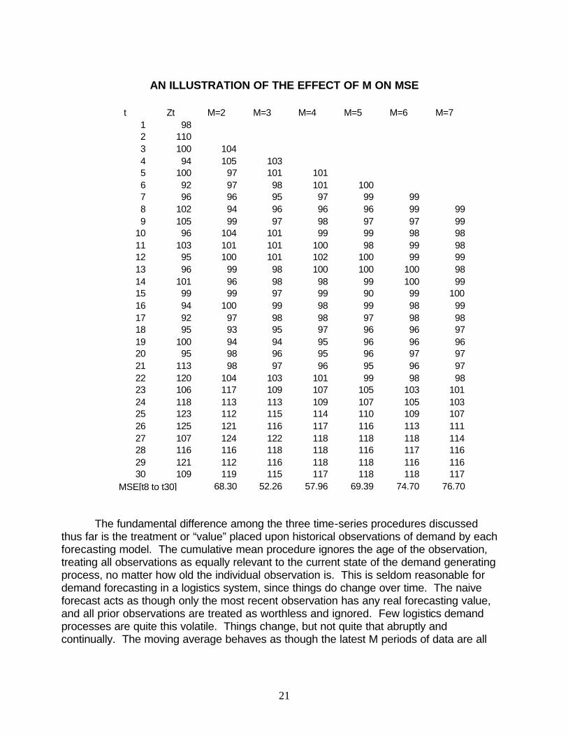
The appropriate value for the parameter M in a given situation is not obvious. If M is "small", the forecast will quickly respond to any "step", or change in level when it does occur, but we lose the "averaging out" effect which would cancel out noise when many observations are included. If M is "large", we get good averaging out of noise, but consequently poorer response to the occurrence of the step change. The optimal value for M in any given situation depends in a fairly complicated way upon the level, the noise variance, and the size and frequency of occurrence of the step or steps in the demand process. In practice, we will not have the detailed prior knowledge of these factors that would be required to choose M optimally. Instead, M is usually selected by trial and error; that is, values of M are tested on historical data, and the value that would have produced the minimum MSE for the historical demand data is used for forecasting. Note that this approach implicitly assumes that these unknown factors are themselves reasonably stationary or time-invariant.

An example of this approach is shown in the table below. Thirty periods of time series data are forecasted with moving averages of periods two through seven. MSEs are calculated over periods eight through thirty. The lowest MSE (52.26) occurs with the three period moving average (M=3). Note from the table of the forecasts that these data underwent a step change in level at period twenty. In effect, the value of M=3 made the best compromise between canceling noise before the step occurred and then reacting to the step once it happened.

20

AN ILLUSTRATION OF THE EFFECT OF M ON MSE

t Zt M=2 M=3 M=4 M=5 M=6 M=7 1 98 2 110 3 100 1044 94 1055 100 976 92 977 96 968 102 949 105 99

10 96 10411 103 10112 95 10013 96 9914 101 9615 99 9916 94 10017 92 9718 95 9319 100 9420 95 9821 113 9822 120 10423 106 11724 118 11325 123 11226 125 12127 107 12428 116 11629 121 11230 109 119

MSE[t8 to t30] 68.30

103 101 101 98 101 100 95 97 99 99 96 96 96 99 99 97 98 97 97 99

101 99 99 98 98 101 100 98 99 98 101 102 100 99 99 98 100 100 100 98 98 98 99 100 99 97 99 90 99 100 99 98 99 98 99 98 98 97 98 98 95 97 96 96 97 94 95 96 96 96 96 95 96 97 97 97 96 95 96 97

103 101 99 98 98 109 107 105 103 101 113 109 107 105 103 115 114 110 109 107 116 117 116 113 111 122 118 118 118 114 118 118 116 117 116 116 118 118 116 116 115 117 118 118 117

52.26 57.96 69.39 74.70 76.70

The fundamental difference among the three time-series procedures discussed thus far is the treatment or “value” placed upon historical observations of demand by each forecasting model. The cumulative mean procedure ignores the age of the observation, treating all observations as equally relevant to the current state of the demand generating process, no matter how old the individual observation is. This is seldom reasonable for demand forecasting in a logistics system, since things do change over time. The naive forecast acts as though only the most recent observation has any real forecasting value, and all prior observations are treated as worthless and ignored. Few logistics demand processes are quite this volatile. Things change, but not quite that abruptly and continually. The moving average behaves as though the latest M periods of data are all

21

equally useful and all older observations are totally worthless. This is a sort of compromise. Note that:

1. The cumulative mean is a moving average where M "expands indefinitely" in the sense that it includes all prior observations and grows with the "length" of the series being forecasted.

2. The naive forecast is a moving average where M = 1.

In this sense, "small" moving averages resemble the naive approach, with all of its strengths and weaknesses. "Large" moving averages resemble the cumulative mean, with all of its advantages and disadvantages.

The Weighted Moving Average

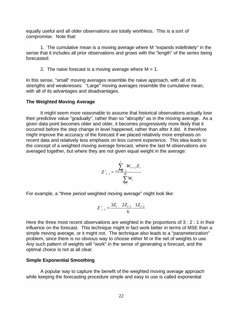
It might seem more reasonable to assume that historical observations actually lose their predictive value "gradually", rather than so "abruptly" as in the moving average. As a given data point becomes older and older, it becomes progressively more likely that it occurred before the step change in level happened, rather than after it did. It therefore might improve the accuracy of the forecast if we placed relatively more emphasis on recent data and relatively less emphasis on less current experience. This idea leads to the concept of a weighted moving average forecast, where the last M observations are averaged together, but where they are not given equal weight in the average:

t

� Wt i - +1Zi = - + 1= i t M'Z t+1 M

�Wi i=1

For example, a "three period weighted moving average" might look like:

'Z t+1

3Zt + 2Zt-1 +1Z = t-2

6

Here the three most recent observations are weighted in the proportions of 3 : 2 : 1 in their influence on the forecast. This technique might in fact work better in terms of MSE than a simple moving average, or it might not. The technique also leads to a "parameterization" problem, since there is no obvious way to choose either M or the set of weights to use. Any such pattern of weights will "work" in the sense of generating a forecast, and the optimal choice is not at all clear.

Simple Exponential Smoothing

A popular way to capture the benefit of the weighted moving average approach while keeping the forecasting procedure simple and easy to use is called exponential

22

smoothing, or occasionally, the “exponentially weighted moving average”. In its simple computational form, we make a forecast for the next period by forming a weighted combination of the last observation and the last forecast:

(1 Z t 'Z t+1 = aZt + - a) '

where a is a parameter called the “smoothing coefficient”, “smoothing factor”, or “smoothing constant”. Values of a are restricted such that 0 < a < 1. The choice of a is up to the analyst. In this form, a can be interpreted as the relative weight given to the most recent data in the series. For example, if an a of 0.2 is used, each successive forecast consists of 20% "new" data (the most recent observation) and 80% "old" data, since the prior forecast is composed of recursively weighted combinations of prior observations. A little algebra on the forecasting model yields a completely equivalent expression that can also be used:

'Z t+1 =Z ' +aett

In this form we can see that exponential smoothing consists of continually updating or refining the most recent forecast of the series by incorporating a fraction of the current forecast error, where a represents that fraction. During periods when the forecast errors are small and unbiased, the procedure has presumably located the current demand level. Adding a fraction of these errors to the forecast will not change it very much. If the errors should become large and biased, this would indicate that the level of demand had changed. Adding in a fraction of these errors will now "move" the forecast toward the new level. Thus exponential smoothing is a kind of feedback system, or an error monitoring and correcting process.

The choice of an appropriate value for a will depend upon the nature of the demand data. In this sense, choice of a in exponential smoothing is analogous to the choice of M in a moving average. If we use a relatively large value for a , we will have "Fast Smoothing"; that is, the forecasts will be highly responsive to true changes in the level of the series when they do occur. Such forecasts will also be "nervous" in the sense that they will also respond strongly to noise. If we use a relatively small value for a , we will have "Slow Smoothing", with sluggish response to changes in the true level of the series. On the other hand, forecasts will be relatively "calm" and unresponsive to the random noise in the demand process. The choice of the optimal value of a in a specific situation is usually done on a trial and error basis so as to minimize MSE on a set of historical data. Experience has shown that when this model is appropriate, optimal a values will typically fall in a range between .1 and .3 .

Another way to think about the choice of a is to consider how a specific choice of a will inflate the forecast error while the data are truly stationary. It can be shown that if the data are simply level and the standard deviation of the noise terms is sn, then the ratio of the forecast RMSE using a given a to the sn will be:

23

RMSE 2a = s 2 -an

For example, using an a value of 0.20 on stationary data "inflates" the RMSE by about five percent. In a sense, this is the price we pay each period to be able to react to a change in the level if and when such a change should appear.

In using exponential smoothing to forecast demand data, there is another issue beyond the choice of a. Since each forecast is a modification of a prior forecast, from where does the initial forecast come? The usual solution to this “initialization” problem is to set the first "forecast" to be equal to the actual demand in the first period:

Z '1 = Z1

after the fact, and to then use exponential smoothing for period 2 and beyond.

Although exponential smoothing is a very simple process, the model is actually more subtle than the arithmetic might suggest. The process is called "exponential" smoothing because each forecast can be shown to be a weighted average of all prior observations, where the weights being employed "decline exponentially" with the increasing age of the observations. Suppose we have been forecasting a series for many periods. At each point in time, we form a forecast such as:

(1 Z t 'Z t+1 = aZt + - a) '

If we are at time t, what does Z't consist of? It is the forecast formed one period ago, at time = t-1:

Z ' t = aZt-1 + -a ) '(1 Z t-1

Substituting this expression for Z't into the equation for Z't+1 yields the equivalent expression:

'Z t+1 = aZt + - a){ aZ + - a ) ' }(1 t -1 (1 Z t -1

Which simplifies to:

(1 2'Z t+1 = aZt + a (1 - a )Z + - a) Z ' }t-1 t-1

Continuing this process of expanding the Z' term on the end of the formula will lead to a general expression:

0 1 2 3'Z t+1 = a(1 - a) Zt + a(1 - a ) Z + a(1 - a ) Zt-2 + a (1 - a ) Zt-3 + .....t-1

24

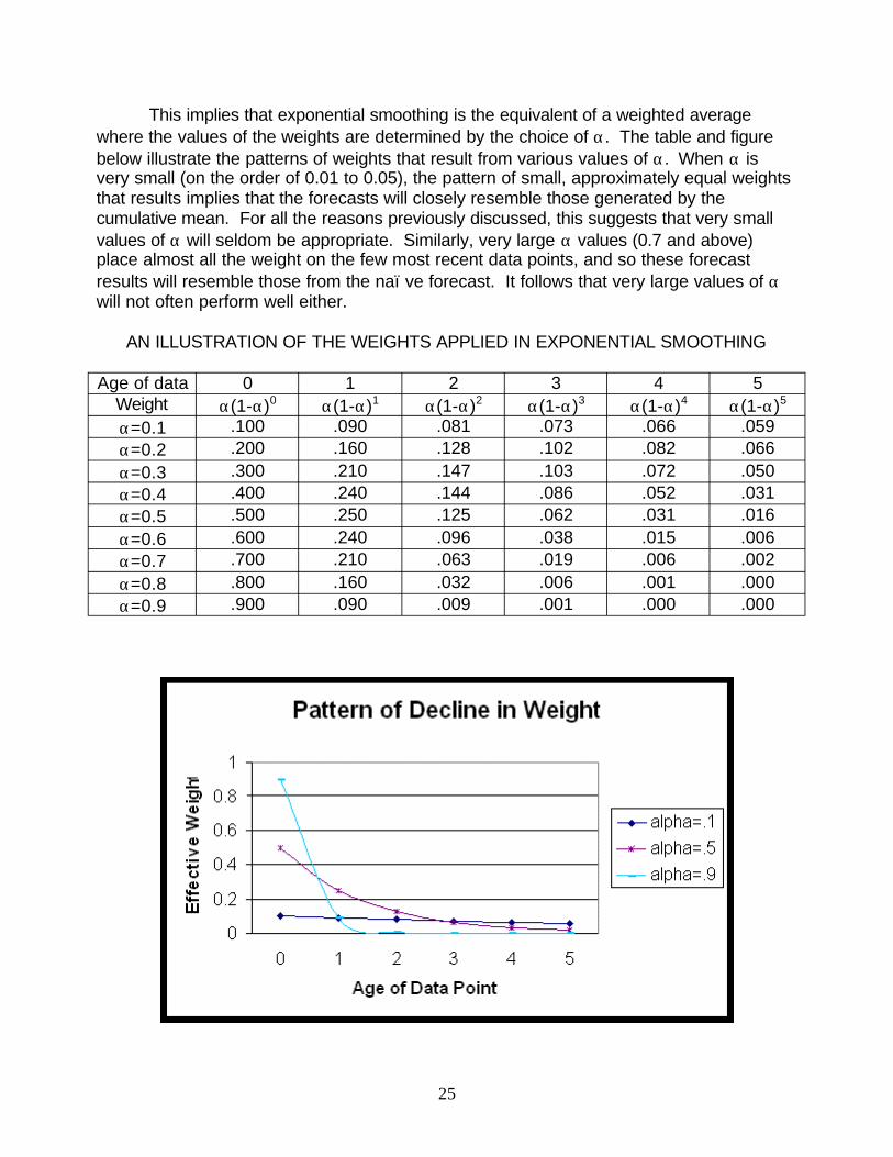
This implies that exponential smoothing is the equivalent of a weighted average where the values of the weights are determined by the choice of a. The table and figure below illustrate the patterns of weights that result from various values of a. When a is very small (on the order of 0.01 to 0.05), the pattern of small, approximately equal weights that results implies that the forecasts will closely resemble those generated by the cumulative mean. For all the reasons previously discussed, this suggests that very small values of a will seldom be appropriate. Similarly, very large a values (0.7 and above) place almost all the weight on the few most recent data points, and so these forecast results will resemble those from the naïve forecast. It follows that very large values of a will not often perform well either.

AN ILLUSTRATION OF THE WEIGHTS APPLIED IN EXPONENTIAL SMOOTHING

Age of data 0 1 2 3 4 5 Weight a(1-a)0 a(1-a)1 a(1-a)2 a(1-a)3 a(1-a)4 a(1-a)5

a=0.1 .100 .090 .081 .073 .066 .059 a=0.2 .200 .160 .128 .102 .082 .066 a=0.3 .300 .210 .147 .103 .072 .050 a=0.4 .400 .240 .144 .086 .052 .031 a=0.5 .500 .250 .125 .062 .031 .016 a=0.6 .600 .240 .096 .038 .015 .006 a=0.7 .700 .210 .063 .019 .006 .002 a=0.8 .800 .160 .032 .006 .001 .000 a=0.9 .900 .090 .009 .001 .000 .000

25

Adaptive Response Rate Exponential Smoothing

Since a small value for a works well while the demand data are "temporarily stationary", but a large value of a works well to correct after a change of level has occurred, the choice of a in simple exponential smoothing is always a compromise between these two competing needs if we expect that the level of the demand data can change from time to time. We could envision a slightly more sophisticated model with two values for a , one large and one small. If the forecasts have been fairly accurate lately, we would use “small a “ to forecast, but if the forecasts have been bad lately, we would use a large value of a, presumably to "catch up" to the change in level which has been causing the recent large errors. This might make sense, but parameterization issues remain. Which two values should we use for a? How "bad" is bad? How "lately" is lately?

Adaptive Response Rate Exponential Smoothing (ARRES), which was proposed by Trigg and Leach, is a technique which embodies this basic idea and avoids the parameterization issue (almost) by allowing a to vary from period to period as a function of the smoothed forecast errors. We start with a fixed smoothing coefficient, b, which is usually set to a value of about 0.2, although once again an appropriate value can be found by experimentation with historical demand data. Given a value for b, we calculate and update Et, which is a smoothed average of our forecast errors:

(1 Et = b et + - b ) Et-1

Et is the "exponentially smoothed equivalent" of the Mean Deviation and is therefore a rolling estimate of the current bias in the forecasts. We also use b to calculate At , which is an exponentially smoothed average of the absolute errors and is therefore a "rolling" estimate of the current MAD:

At = b | e | + - b ) A(1 t t-1

Then we use Et and At to set at, which is a value of a that is appropriate given the current forecast accuracy:

=| E At |a t t

and we use at to generate a forecast:

Z (1 t Z t 'Z t+1 = at t + - a ) '

In this way at will automatically adapt or respond to the forecast errors, taking on large values when large, biased errors occur and taking on small values when small and unbiased errors are generated. While adaptive procedures such as this are intuitively very

26

plausible, experience with them in actual logistics system applications has shown that they tend to be too "nervous" or "over-reactive". The resulting instability in the at values often leads to forecasts that are no more accurate than those which would have been obtained with simple exponential smoothing.

Extending the Forecast Horizon

In each of the models considered so far, we have focused on developing a "one period ahead" forecast. That is, at time t we develop an expression for Z’t+1. In many cases it will be useful to extend the forecast two or more periods into the future. For each of the models developed thus far, the forecast developed at time t holds indefinitely into the future:

'Z t+k = Z ' t+1 , for all k > 1

This is true because in these models the underlying demand process is assumed to be simply stationary, or "temporarily stationary", or a random walk. As such, we have no additional information or reason to modify our forecast based on the length of the forecasting horizon. On the other hand, if the demand process is subject to changes in level (or is random walk), then we would expect the forecast accuracy to decline as we extend the forecasting horizon. An MSE that is calculated on weekly forecasts that were made, for example, eight weeks in advance could be much higher than the MSE on forecasts made only one week in advance. This happens, in one sense, because the long forecasting horizon allows much more opportunity for the demand level to change between the time the forecast for a given period was made and the time when the demand actually occurs.

Trended Demand Data

Many items in a logistics system can be expected to shown a trend in demand. None of the models discussed thus far will cope well with a trended demand generation process. Models such as the ones we have seen, which are intended to forecast stationary data, will lag badly behind trended data, showing poor accuracy and high bias. Consider a completely noiseless data series with a simple, constant, linear trend. This should be a very simple pattern to forecast. As is shown in the figure below, neither a moving average nor exponential smoothing will produce a useful forecast. The problem is that any such procedure is averaging together "old" data, all of which is unrepresentative of the "future level" of the series. It is as though the series undergoes a change in level in each period, and the forecast never has a chance to adapt to it or to "catch up."

27

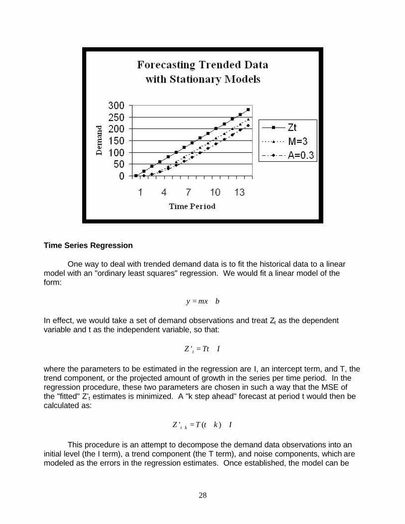
Time Series Regression

One way to deal with trended demand data is to fit the historical data to a linear model with an "ordinary least squares" regression. We would fit a linear model of the form:

y = mx b+

In effect, we would take a set of demand observations and treat Zt as the dependent variable and t as the independent variable, so that:

Z ' t = Tt I+

where the parameters to be estimated in the regression are I, an intercept term, and T, the trend component, or the projected amount of growth in the series per time period. In the regression procedure, these two parameters are chosen in such a way that the MSE of the "fitted" Z’t estimates is minimized. A "k step ahead" forecast at period t would then be calculated as:

+ ( +Z ' t k = T t k ) + I

This procedure is an attempt to decompose the demand data observations into an initial level (the I term), a trend component (the T term), and noise components, which are modeled as the errors in the regression estimates. Once established, the model can be

28

used for several periods, or it could be updated and re-estimated as each new data point is observed. Given the current state of computer capability, the computational burden implied by this continual updating need not be excessive. On the other hand, this regression-based approach suffers from the same potential problem as do the cumulative mean and simple moving average. In a simple regression, each observation, no matter how old, is given the same weight or influence in determining the regression coefficients, and hence, the value of the next forecast. However, there is always the possibility that the series can undergo a shift in “level” at some point, or that the slope of the trend line may change. Once such a change has occurred, all of the "older" data are unrepresentative of the future of the process. This logic suggests that perhaps some weighting scheme should be used to "discount" the older data and place more emphasis on more recent observations. This might be done, for example, with a "Weighted Least Squares" regression. While this could be done, in actual practice other, simpler procedures are more commonly used that accomplish the same ends.

Brown’s Double Smoothing

If we refer again to the data in the previous figure, we can see that although the forecasts lag badly behind the actual data, both the moving average and the exponential smoothing forecasts do capture the true rate of growth in the series. The amount by which the forecast lags is basically a function of how fast the series is growing and how far back the data is being averaged, which is in turn a function of the M value or a value being used. It is possible to use this insight to develop a smoothing procedure that will separate the trend component from the noise in the series and forecast trended data without a lag. One such procedure, which has been popularized by R.G. Brown, is called Double Exponential Smoothing, or Double Smoothing. Given a smoothing coefficient of a, we first calculate a simple smoothed average of the data:

(1 Bt+1 = a Zt + -a )Bt

This series will follow the slope of the original data while smoothing out some of the noise. A second series is then formed by smoothing the Bt values:

(1 Ct+1 = aBt + - a )Ct

The second series will also tend to capture the slope of the original data while further smoothing the noise. Now we can use these two smoothed values to form the forecast:

-t t'Z t+1 = 2B Ct a (B C )

- + t 1 -a

It has been demonstrated that performing double smoothing on a data set is mathematically equivalent to forecasting with a rolling (or continually updated) weighted least squares regression where the weights being applied would be of the form:

29

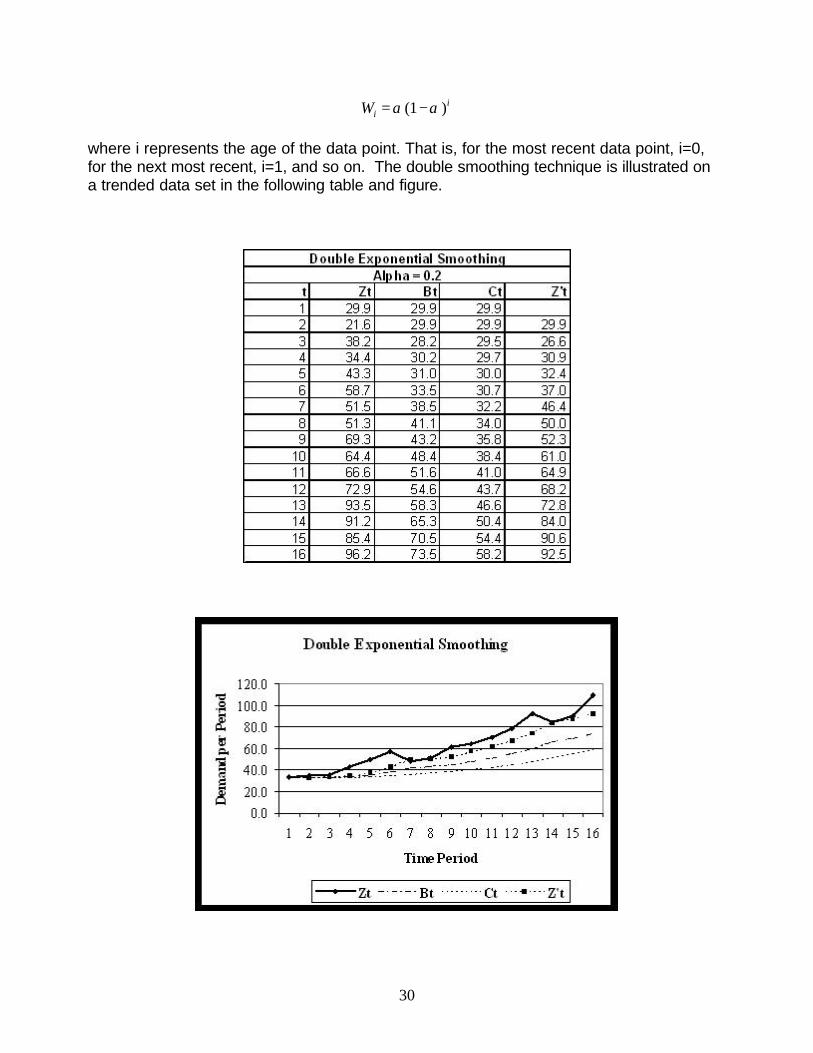
Wi = a (1 -a )i

where i represents the age of the data point. That is, for the most recent data point, i=0, for the next most recent, i=1, and so on. The double smoothing technique is illustrated on a trended data set in the following table and figure.

30

--

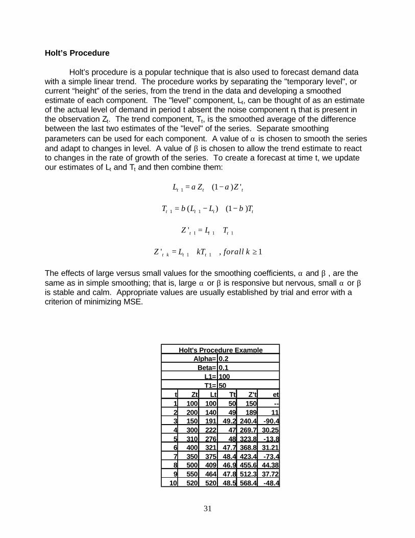
Holt’s Procedure

Holt’s procedure is a popular technique that is also used to forecast demand data with a simple linear trend. The procedure works by separating the "temporary level", or current “height” of the series, from the trend in the data and developing a smoothed estimate of each component. The "level" component, Lt, can be thought of as an estimate of the actual level of demand in period t absent the noise component nt that is present in the observation Zt. The trend component, Tt, is the smoothed average of the difference between the last two estimates of the "level" of the series. Separate smoothing parameters can be used for each component. A value of a is chosen to smooth the series and adapt to changes in level. A value of b is chosen to allow the trend estimate to react to changes in the rate of growth of the series. To create a forecast at time t, we update our estimates of Lt and Tt and then combine them:

(1 Z tLt+1 = a Zt + - a) '

(1 Tt+1 = b (L - L ) + - b )Tt+1 t t

'Z t+1 = Lt+1 + Tt+1

'Z t+k = Lt+1 + kTt+1 , forall k ‡ 1

The effects of large versus small values for the smoothing coefficients, a and b , are the same as in simple smoothing; that is, large a or b is responsive but nervous, small a or b is stable and calm. Appropriate values are usually established by trial and error with a criterion of minimizing MSE.

Holt's Procedure Example Alpha= 0.2

Beta= 0.1 L1= 100 T1= 50

t Zt Lt Tt Z't et 1 100 100 50 150 2 200 140 49 189 11 3 150 191 49.2 240.4 -90.4 4 300 222 47 269.7 30.25 5 310 276 48 323.8 -13.8 6 400 321 47.7 368.8 31.21 7 350 375 48.4 423.4 -73.4 8 500 409 46.9 455.6 44.38 9 550 464 47.8 512.3 37.72

10 520 520 48.5 568.4 -48.4

31

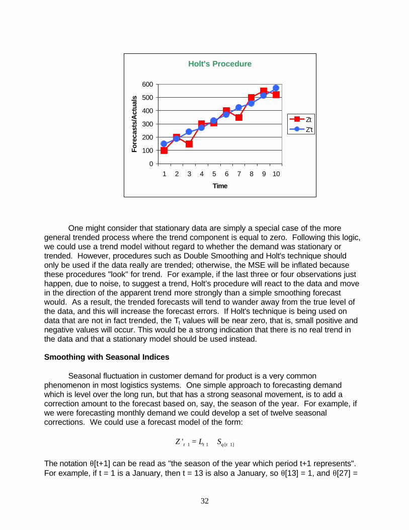
Holt's Procedure

Fore

cast

s/A

ctua

ls

600

500

400

300

200

100

0

1 2 3 4 5 6 7 8 9 10

Time

Zt

Z't

One might consider that stationary data are simply a special case of the more general trended process where the trend component is equal to zero. Following this logic, we could use a trend model without regard to whether the demand was stationary or trended. However, procedures such as Double Smoothing and Holt's technique should only be used if the data really are trended; otherwise, the MSE will be inflated because these procedures "look" for trend. For example, if the last three or four observations just happen, due to noise, to suggest a trend, Holt’s procedure will react to the data and move in the direction of the apparent trend more strongly than a simple smoothing forecast would. As a result, the trended forecasts will tend to wander away from the true level of the data, and this will increase the forecast errors. If Holt's technique is being used on data that are not in fact trended, the Tt values will be near zero, that is, small positive and negative values will occur. This would be a strong indication that there is no real trend in the data and that a stationary model should be used instead.

Smoothing with Seasonal Indices

Seasonal fluctuation in customer demand for product is a very common phenomenon in most logistics systems. One simple approach to forecasting demand which is level over the long run, but that has a strong seasonal movement, is to add a correction amount to the forecast based on, say, the season of the year. For example, if we were forecasting monthly demand we could develop a set of twelve seasonal corrections. We could use a forecast model of the form:

'Z t+1 = Lt+1 + Sq [t+1]

The notation q[t+1] can be read as "the season of the year which period t+1 represents". For example, if t = 1 is a January, then t = 13 is also a January, so q[13] = 1, and q[27] =

32

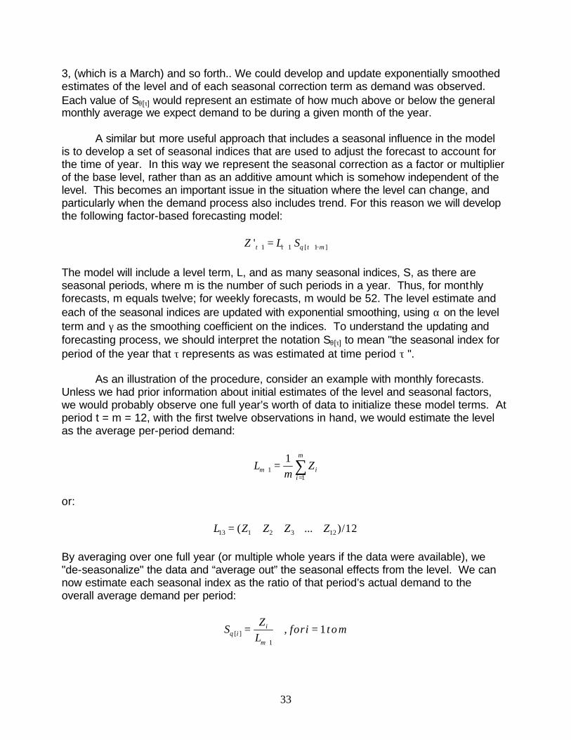
3, (which is a March) and so forth.. We could develop and update exponentially smoothed estimates of the level and of each seasonal correction term as demand was observed. Each value of Sq[t] would represent an estimate of how much above or below the general monthly average we expect demand to be during a given month of the year.

A similar but more useful approach that includes a seasonal influence in the model is to develop a set of seasonal indices that are used to adjust the forecast to account for the time of year. In this way we represent the seasonal correction as a factor or multiplier of the base level, rather than as an additive amount which is somehow independent of the level. This becomes an important issue in the situation where the level can change, and particularly when the demand process also includes trend. For this reason we will develop the following factor-based forecasting model:

'Z t+1 = L Sq [ 1 ]t+1 t+ -m

The model will include a level term, L, and as many seasonal indices, S, as there are seasonal periods, where m is the number of such periods in a year. Thus, for mont hly forecasts, m equals twelve; for weekly forecasts, m would be 52. The level estimate and each of the seasonal indices are updated with exponential smoothing, using a on the level term and g as the smoothing coefficient on the indices. To understand the updating and forecasting process, we should interpret the notation Sq[t] to mean "the seasonal index for period of the year that t represents as was estimated at time period t ".

As an illustration of the procedure, consider an example with monthly forecasts. Unless we had prior information about initial estimates of the level and seasonal factors, we would probably observe one full year’s worth of data to initialize these model terms. At period t = m = 12, with the first twelve observations in hand, we would estimate the level as the average per-period demand:

m1

m Lm+1 = �Zi

i =1

or:

1 3 ... L13 = (Z + Z2 + Z + + Z12 )/12

By averaging over one full year (or multiple whole years if the data were available), we "de-seasonalize" the data and “average out” the seasonal effects from the level. We can now estimate each seasonal index as the ratio of that period’s actual demand to the overall average demand per period:

Sq [ ] = Zi , fori = 1 t o m

Li m+1

33

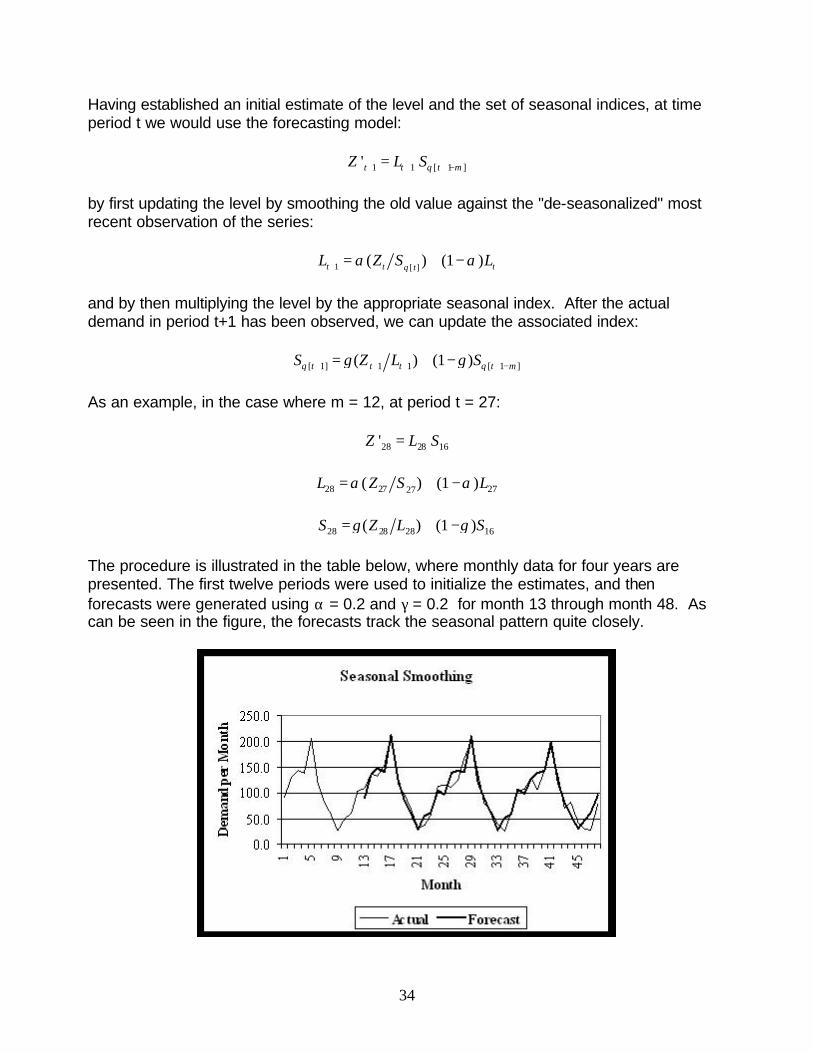
Having established an initial estimate of the level and the set of seasonal indices, at time period t we would use the forecasting model:

'Z t+1 = L Sq [ 1 ]t+1 t+ -m

by first updating the level by smoothing the old value against the "de-seasonalized" most recent observation of the series:

(1 Lt+1 = a(Z St q [ ] ) + - a)Lt t

and by then multiplying the level by the appropriate seasonal index. After the actual demand in period t+1 has been observed, we can update the associated index:

(1 t+1 1Sq [t+1] = g (Z Lt+1) + - g )Sq [t+ -m ]

As an example, in the case where m = 12, at period t = 27:

Z '28 = L S1628

L28 = a( (1 ) + -a)LZ S 27 27 27

S28 = g ( (1 ) + -g )SZ L 28 28 16

The procedure is illustrated in the table below, where monthly data for four years are presented. The first twelve periods were used to initialize the estimates, and then forecasts were generated using a = 0.2 and g = 0.2 for month 13 through month 48. As can be seen in the figure, the forecasts track the seasonal pattern quite closely.

34

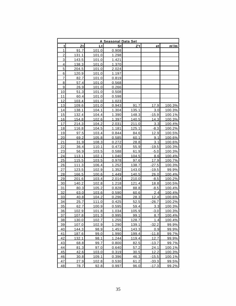
123456789

101112131415161718192021222324252627282930313233343536373839404142434445464748

A Seasonal Data Set t Zt Lt St Z't et m'/m

91.7 101.0 0.908 131.1 101.0 1.298 143.5 101.0 1.421 138.3 101.0 1.370 204.5 101.0 2.024 120.9 101.0 1.197

82.7 101.0 0.819 57.4 101.0 0.568 26.9 101.0 0.266 51.3 101.0 0.508 60.4 101.0 0.598

103.4 101.0 1.023 109.6 101.0 0.943 91.7 17.9 100.3% 138.1 104.1 1.304 135.1 3.0 100.3% 132.4 104.4 1.390 148.3 -15.9 100.1% 154.8 102.6 1.397 140.5 14.3 100.3% 214.3 104.2 2.031 211.0 3.3 100.4% 116.8 104.5 1.181 125.1 -8.3 100.2%

97.5 103.4 0.844 84.6 12.9 100.5% 69.2 105.8 0.585 60.1 9.1 100.6% 31.9 108.3 0.272 28.8 3.1 100.6% 36.4 110.1 0.473 55.9 -19.5 100.3% 56.9 103.5 0.588 61.9 -5.0 100.3%

113.1 102.1 1.040 104.5 8.6 100.4% 115.5 103.5 0.978 97.6 17.9 100.7% 111.3 106.4 1.252 138.7 -27.5 100.3% 123.5 102.9 1.352 143.0 -19.5 99.9% 166.5 100.6 1.449 140.5 26.0 100.4% 201.6 103.4 2.014 210.0 -8.5 100.2% 140.2 102.8 1.218 121.4 18.8 100.5%

80.3 105.2 0.828 88.8 -8.5 100.4% 63.0 103.6 0.590 60.6 2.4 100.4% 40.8 104.2 0.296 28.3 12.4 100.6% 25.7 111.0 0.425 52.5 -26.7 100.2% 62.7 100.9 0.595 59.4 3.3 100.3%

102.9 101.8 1.034 105.9 -3.0 100.3% 107.8 101.3 0.995 99.1 8.7 100.4% 130.0 102.7 1.255 128.7 1.4 100.4% 107.0 102.9 1.290 139.1 -32.2 99.9% 144.3 98.9 1.451 143.3 0.9 99.9% 187.6 99.0 1.990 199.4 -11.8 99.7% 132.1 98.1 1.244 119.4 12.7 99.9%

68.8 99.7 0.800 82.5 -13.7 99.7% 81.3 97.0 0.640 57.2 24.1 100.1% 42.6 103.0 0.319 30.5 12.2 100.3% 30.8 109.1 0.396 46.3 -15.5 100.1% 27.9 102.8 0.530 61.2 -33.3 99.5% 78.7 92.8 0.997 96.0 -17.3 99.2%

35

One final adjustment is often made to this procedure. Notice that, due to the manner in which we initialize the seasonal indices, the sum of the indices must equal m, or in other words, the average of the indices must equal one. This makes sense; it is the equivalent of saying that the average month must be equal to the average month. However, once we begin the updating process, we change the indices one at a time. For this reason, the sum of the indices will no longer necessarily equal m. For example, in the table above, the last column shows the sum of the twelve most recent index values expressed as a percentage of m. If the sum of the indices is allowed to wander away from m, biased forecasts will result. The final step in the procedure, then, is to "normalize" the index values. In this context, normalization means that when one index value is updated, all the other index values are adjusted so that their sum always equals m. The specific adjustment mechanism is arbitrary. A typical procedure would be:

1. Take the amount that the update has added to the new value of the seasonal index,

2. Apportion it out to the other (m-1) indices, and

3. Subtract it from the (m-1) indices in such a way that the (m-1) estimates maintain their same relative proportion, and the sum of all the indices is still m.

If we had a set of seasonal indices, say, S1 through Sm, and an update of an index results in an increment of d being added to, for example, St , then the new set of indices, S’1

through S’m would be calculated as:

S ' t = St + d

S ' i = Si -d Si , for all i „ t

m S- t

Winter’s Model for Seasonal/Trended Demand

It will often be the case that items in a logistics system exhibit demand patterns that include both trend and seasonality. It is possible to combine the logic of Holt’s procedure for trended data and the seasonal index approach so as to forecast level, trend, and seasonality. This approach is embodied in Winter's Model for Trended/Seasonal Data. Each component term of the forecast is estimated with exponential smoothing, and separate smoothing coefficients, a , b , and g , can be used for each estimate:

1 'Z t+1 = (Lt+1 + Tt+1) Sq [ t+ -m]

Lt+1 = a(Z Sq [ ]) + (1 - a)( L T )t t t + t

(1 Tt+1 = b (L - L ) + - b )Tt+1 t t

36

(1 Sq [t+1] = g (Zt+1 1Lt+1) + - g )Sq [t+ -m ]

Developing reasonable initial estimates of the L, T, and S values is more difficult in this procedure. Unless we have some good a priori reason to establish these values, we will need at least two full seasons of historical data (usually two years worth) to be able to distinguish between trend and seasonality in the data. As an example, a simple but approximate approach is as follows.

Given two years of monthly data (Z1 through Z24), we can compute Y1 as the average monthly demand of the first year and Y2 as the average monthly demand of the second year. Since averaging over a year de-seasonalizes the data, and also allows some of the noise to cancel, the difference between Y1 and Y2 can be roughly attributed to one year’s accumulation of trend, so an initial estimate of T can be calculated:

m1

m Y1 = �Zi

i=1

m1 2m

Y2 = � Zi = +1i m

Y Y1-2T = m

The first year average, Y1, can be thought of as the average of the initial level plus eleven months with increasing trend. In other words, if we ignore seasonality and noise:

( L T ) ( L T L m -1} ) Y1

L + + + + 2 ) + ...( { T =

m

or:

Y1 = + + + + ....{ m - 1})mL T (1 2 3

m m

An estimate of the initial level can therefore be:

(L Y1 -

T m -1)= 1 2

The seasonal influence can be initially estimated from the difference between the actual demand observed in a period and an estimate based only on level and trend. For each of the m periods in a year, we have two observations to average, so:

37

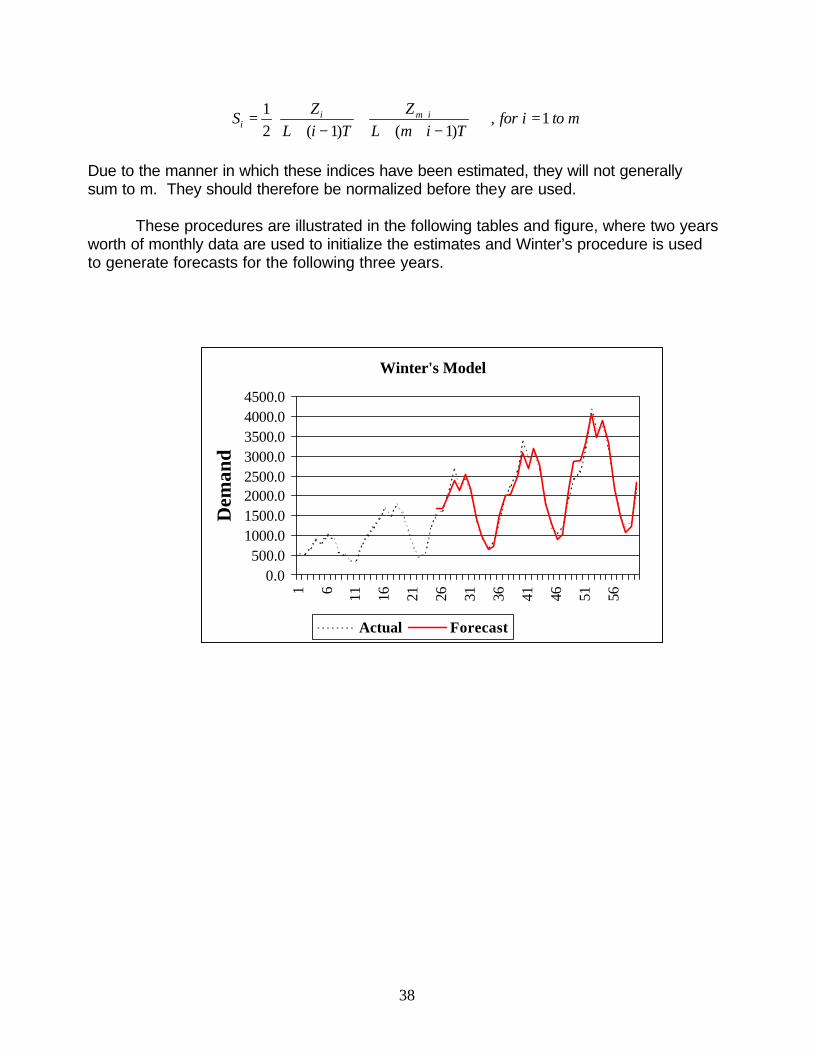
ø+Si = 1 Ø Zi +

Zm i œ , for i =1 to m

2 Œ L + (i - 1) T L + (m + - 1)T ߺ i

Due to the manner in which these indices have been estimated, they will not generally sum to m. They should therefore be normalized before they are used.

These procedures are illustrated in the following tables and figure, where two years worth of monthly data are used to initialize the estimates and Winter’s procedure is used to generate forecasts for the following three years.

Winter's Model

0.0 500.0

1000.0 1500.0 2000.0 2500.0 3000.0 3500.0 4000.0 4500.0

1 6 11 16 21 26 31 36 41 46 51 56

Dem

and

Actual Forecast

38

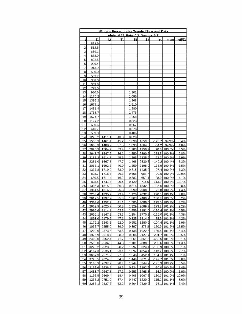
123456789

101112131415161718192021222324252627282930313233343536373839404142434445464748495051525354555657585960

Winter's Procedure for Trended/Seasonal Data Alpha=0.25, Beta=0.3, Gamma=0.2

t Zt Lt Tt St Z't et m'/m |et|/Zt 533.9 512.5 659.1 878.9 802.5 999.4 913.9 590.0 503.7 368.0 369.8 775.0 980.6 1.101

1175.2 1.096 1396.2 1.268 1677.1 1.510 1481.4 1.280 1758.7 1.475 1574.7 1.268 1127.2 0.823 680.6 0.567 446.7 0.378 569.8 0.406

1228.2 1411.1 43.0 0.828 1530.3 1461.4 45.2 1.090 1659.0 -128.7 99.9% 8.4% 1600.3 1480.9 37.5 1.093 1664.5 -64.2 99.9% 4.0% 2020.9 1504.7 33.4 1.283 1950.9 70.0 100.0% 3.5% 2648.7 1547.2 36.1 1.550 2390.2 258.5 100.3% 9.8% 2188.3 1614.7 45.5 1.295 2125.6 62.7 100.5% 2.9% 2381.0 1667.5 47.7 1.466 2530.3 -149.2 100.4% 6.3% 2065.1 1692.6 40.9 1.259 2198.9 -133.9 100.3% 6.5% 1337.8 1710.2 33.9 0.815 1435.2 -97.4 100.2% 7.3% 898.7 1718.6 26.3 0.558 988.7 -90.0 100.2% 10.0% 680.5 1711.4 16.2 0.382 652.4 28.0 100.2% 4.1% 828.4 1741.5 20.4 0.420 714.5 113.9 100.3% 13.7%

1396.3 1815.0 36.3 0.816 1532.9 -136.6 100.2% 9.8% 1981.5 1816.2 25.8 1.090 2008.3 -26.8 100.2% 1.4% 2253.4 1835.7 23.9 1.120 2032.9 220.5 100.4% 9.8% 2617.5 1897.7 35.3 1.303 2480.7 136.8 100.6% 5.2% 3364.6 1952.2 41.1 1.585 3089.6 275.0 100.9% 8.2% 2962.9 2025.7 50.8 1.329 2689.7 273.2 101.2% 9.2% 2995.6 2114.8 62.3 1.456 3191.0 -195.4 101.1% 6.5% 2655.1 2147.3 53.3 1.254 2770.2 -115.0 101.1% 4.3% 1893.0 2179.6 47.1 0.825 1814.2 78.9 101.1% 4.2% 1176.2 2243.3 52.0 0.551 1280.6 -104.4 101.1% 8.9% 1036.7 2255.0 39.9 0.397 875.8 160.9 101.2% 15.5% 1209.0 2373.6 63.5 0.438 1022.6 186.4 101.4% 15.4% 1925.9 2518.7 88.0 0.806 2127.7 -201.7 101.3% 10.5% 2402.0 2552.4 71.7 1.061 2861.5 -459.5 101.0% 19.1% 2596.0 2534.3 44.8 1.101 2888.6 -292.6 100.9% 11.3% 3223.2 2523.8 28.2 1.297 3324.1 -100.9 100.8% 3.1% 4167.3 2535.1 23.1 1.597 4054.1 113.2 100.9% 2.7% 3637.3 2571.2 27.0 1.346 3452.4 184.8 101.1% 5.1% 3728.5 2624.3 34.8 1.449 3871.2 -142.7 101.0% 3.8% 3168.9 2637.7 28.4 1.244 3344.2 -175.3 100.9% 5.5% 2162.6 2636.5 19.5 0.824 2192.6 -30.0 100.9% 1.4% 1483.7 2647.8 17.1 0.553 1468.8 14.9 100.9% 1.0% 1198.5 2669.4 18.4 0.408 1067.8 130.7 101.0% 10.9% 1335.2 2751.0 37.4 0.447 1220.0 115.2 101.1% 8.6% 2253.1 2837.8 52.2 0.804 2329.2 -76.1 101.1% 3.4%

39

Once again, it can be important to normalize each seasonal index as the forecasting proceeds. As was true with the models for trended data, seasonal procedures should only be used on data that are truly seasonal; otherwise, the MSE can be inflated. If we use a seasonal technique on data that are not seasonal, then all the Sq[t] values will be "near" 1.0 all of the time.

While Winter’s procedure is not complex, there can be quite a bit of tedious calculation involved. To forecast weekly demand data, for example, we would first select appropriate values of a , b , and g as smoothing parameters. This would involve a simultaneous search of possible combinations of values. At each weekly forecast, we would update estimates of Lt, Tt, and the appropriate Sq[t], and then normalize the other 51 seasonal indices. Needless to say, in practice this work is done in a computer. Most commercial software intended to forecast demand in a logistics system incorporates this procedure or some variation on it.

Forecasting Low Density Demand

Many items in a logistics system can be expected to exhibit low density of demand; that is, the demand for a specific SKU at a specific location over a relatively short time interval will be small or sparse. This can often occur, for example, at the retail level in consumer goods, and in the case of maintenance, repair, and operating supplies (MRO items) in industrial systems. In situations where demand is sporadic and often is zero in any given period, time-series procedures as discussed above are usually inappropriate. Error measures such as MAPE, for example, are ill defined when the actual demand that occurs is zero. If the usual forecast being generated by the forecasting model is simply zero, why are we carrying the item? How will our inventory control logic handle an item when its projected demand is zero?

Another forecasting approach is called for. Instead of working with historical data to estimate the current expected value of the generating process (Z’t+1) and using the observed forecast errors to estimate a standard deviation, another approach is to directly estimate the demand probability distribution. In this case, the "forecast" becomes the current estimation of the entire probability distribution, rather than a point estimate of the next period demand.

The Poisson Distribution

This discrete, non-negative distribution is often appropriate to describe the probability of "rare" events. For example, if demand arises from a failure process, as in repair parts, there is theoretical justification for the Poisson. Many mechanical and electronic components follow a failure process such that the "time to failure", or component lifetime, will follow the exponential probability distribution. For a set of such items, the number failing per unit time will follow the Poisson.

The Poisson can also be a reasonable choice for a demand distribution in the case where a relatively large number of customers all have a given probability of purchasing an

40

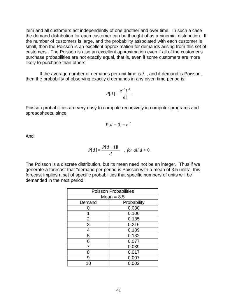
item and all customers act independently of one another and over time. In such a case the demand distribution for each customer can be thought of as a binomial distribution. If the number of customers is large, and the probability associated with each customer is small, then the Poisson is an excellent approximation for demands arising from this set of customers. The Poisson is also an excellent approximation even if all of the customer's purchase probabilities are not exactly equal, that is, even if some customers are more likely to purchase than others.

If the average number of demands per unit time is l , and if demand is Poisson, then the probability of observing exactly d demands in any given time period is:

e -lld

[ ] =P d d !

Poisson probabilities are very easy to compute recursively in computer programs and spreadsheets, since:

[P d = 0] = e -l

And:

P d -1]l[ ] = , for all d > 0P d

[

d

The Poisson is a discrete distribution, but its mean need not be an integer. Thus if we generate a forecast that "demand per period is Poisson with a mean of 3.5 units", this forecast implies a set of specific probabilities that specific numbers of units will be demanded in the next period:

Poisson Probabilities Mean = 3.5

Demand Probability 0 0.030 1 0.106 2 0.185 3 0.216 4 0.189 5 0.132 6 0.077 7 0.039 8 0.017 9 0.007 10 0.002

41

The variance of the Poisson distribution is always equal to l, so this single parameter completely describes the distribution. As l becomes large (l >25), the Poisson converges to a discrete approximation to the Normal distribution. To estimate demand with the Poisson, one usually gathers historical observations of demand per period and averages them to estimate l. Note that this is the equivalent of the "cumulative average approach" with all of its inherent assumptions of extreme stability in the demand process over time. To react to potential movements in the generating process, one might operate Exponential Smoothing on the observed data and use the resulting forecast as the current estimate of the mean of the Poisson process. In this case it would be important to maintain several decimal places in the estimate instead of rounding the average to an integer value.

Compound Poisson Distributions

It is frequently the case that the observed demand data display more variance than would be expected from the Poisson distribution; that is, the observed demand variance is substantially greater than the mean demand. In this situation a set of related distributions may be appropriate. For example, the Gamma-Poisson, also called the Negative Binomial, is a discrete, non-negative "Poisson-like" distribution that can have any variance greater than its mean. The Gamma-Poisson distribution would model the case where demand in any given period is Poisson, but the mean of the Poisson varies over time as though in each period it were an independent realization from a Gamma probability distribution. Given that a random variable is Gamma-Poisson distributed with a mean of m and a variance of s2, the distribution parameters, a , b , and r , are defined as:

2sb =

m

a b 1= -

m r =

a

We follow the parameter notation here that is conventional in the field; these parameters are in no way related to the exponential smoothing coefficients a and b. In using the Gamma-Poisson distribution, probabilities can be easily calculated from the following recursive formulae:

[ -rP d = 0] = b

And:

42

[ ] = P d -1] a r + -1)

, for all d > 0P d [( d

d b

One would typically use historical observations to estimate the mean and variance of observed demand to estimate the parameters of the distribution. Once again, the use of very long-term averages for these estimates implies an assumption of underlying stationarity in the demand process that may or may not be appropriate.

Empirical Distributions and Vector Smoothing

A third approach is to simply fit the observed demand data to an arbitrary empirical distribution. If, for example, over N periods we observed that demand was zero exactly n0

times, and that demand in a period was exactly one on n1 occasions, and so forth, we would estimate that:

P d = = = ni[ i] Pi N

Once again we have the problem of updating these estimates to reflect changes in the underlying demand distribution which may occur over time. An approach to this problem that has been developed by R.G. Brown is called "Vector Smoothing".

Given a set of historical demand data, we could establish initial estimates of the set of Pi values as described above. Then as new demand data were observed, each Pi

estimate would be updated using Vector Smoothing as follows:

P t (1 [ „[ ] = a(0) + - a)P t -1] , for all i Zti i

P t (1 [ =[ ] = a(1) + - a)P t -1] , for all i Zti i

So long as the initial Pi estimates sum to 1.0, this procedure will generate new Pi[t] estimates that will also sum to 1.0 at each time period. The choice of a large or small value for a will determine how quickly or how slowly the probability estimates will change in response to changes in the observed frequencies of the demanded quantities.

Other Time Series Procedures

Many other more sophisticated time-series forecasting procedures are available, and many have been applied to the problem of forecasting demand in a logistics system. We will discuss two of the more well known approaches, Power Spectrum Analysis and the Box-Jenkins procedure. Our treatment of each will be introductory, brief, and non­technical.

43

�

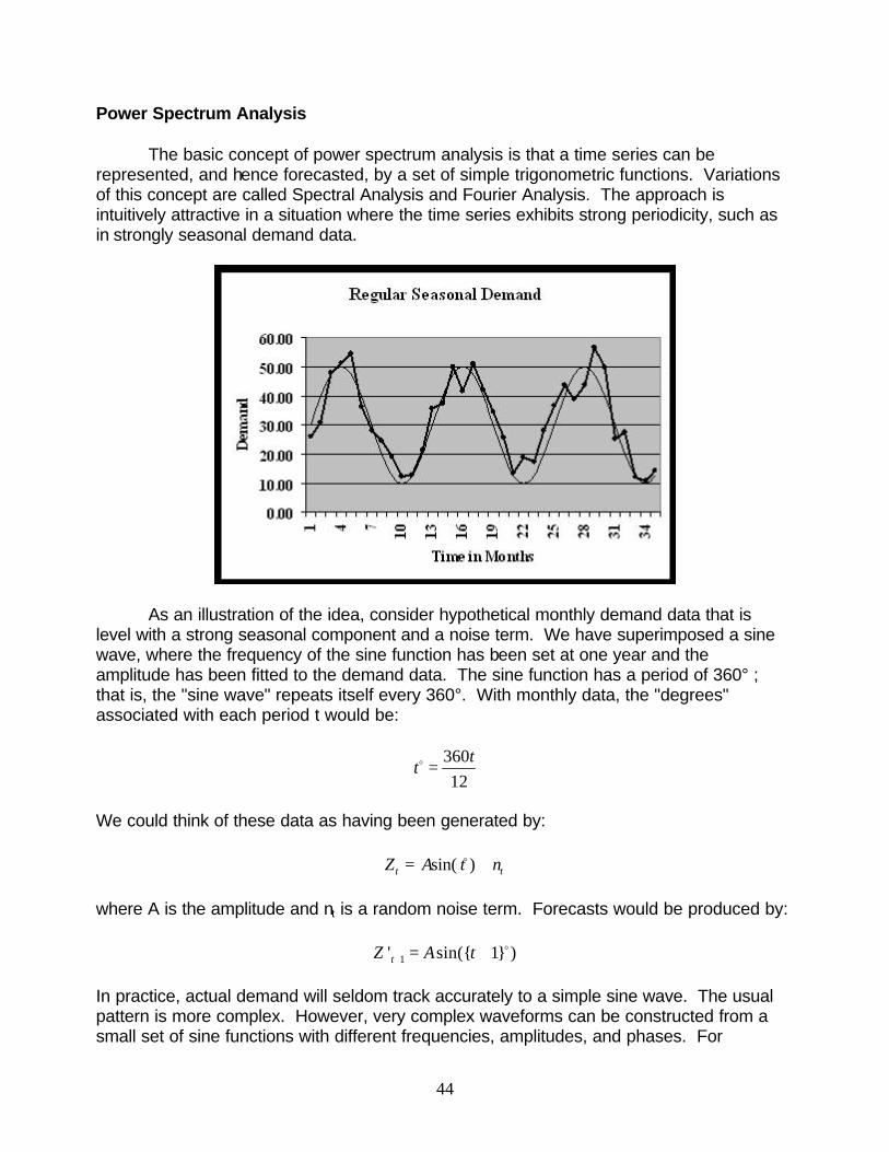
Power Spectrum Analysis

The basic concept of power spectrum analysis is that a time series can be represented, and hence forecasted, by a set of simple trigonometric functions. Variations of this concept are called Spectral Analysis and Fourier Analysis. The approach is intuitively attractive in a situation where the time series exhibits strong periodicity, such as in strongly seasonal demand data.

As an illustration of the idea, consider hypothetical monthly demand data that is level with a strong seasonal component and a noise term. We have superimposed a sine wave, where the frequency of the sine function has been set at one year and the amplitude has been fitted to the demand data. The sine function has a period of 360° ; that is, the "sine wave" repeats itself every 360°. With monthly data, the "degrees" associated with each period t would be:

t� = 360t 12

We could think of these data as having been generated by:

t�Zt = Asin( ) + nt

where A is the amplitude and nt is a random noise term. Forecasts would be produced by:

'Z t+1 = A sin({ t + 1} )

In practice, actual demand will seldom track accurately to a simple sine wave. The usual pattern is more complex. However, very complex waveforms can be constructed from a small set of sine functions with different frequencies, amplitudes, and phases. For

44

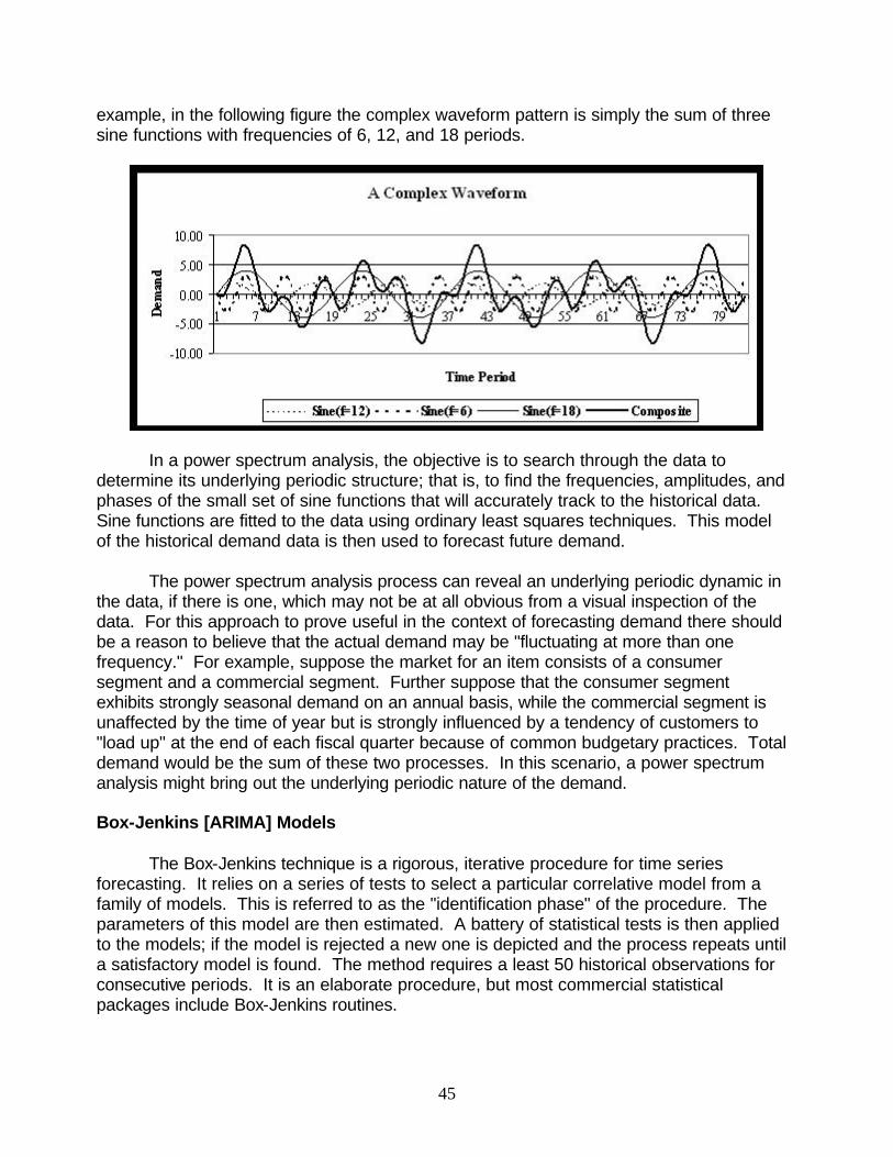
example, in the following figure the complex waveform pattern is simply the sum of three sine functions with frequencies of 6, 12, and 18 periods.

In a power spectrum analysis, the objective is to search through the data to determine its underlying periodic structure; that is, to find the frequencies, amplitudes, and phases of the small set of sine functions that will accurately track to the historical data. Sine functions are fitted to the data using ordinary least squares techniques. This model of the historical demand data is then used to forecast future demand.

The power spectrum analysis process can reveal an underlying periodic dynamic in the data, if there is one, which may not be at all obvious from a visual inspection of the data. For this approach to prove useful in the context of forecasting demand there should be a reason to believe that the actual demand may be "fluctuating at more than one frequency." For example, suppose the market for an item consists of a consumer segment and a commercial segment. Further suppose that the consumer segment exhibits strongly seasonal demand on an annual basis, while the commercial segment is unaffected by the time of year but is strongly influenced by a tendency of customers to "load up" at the end of each fiscal quarter because of common budgetary practices. Total demand would be the sum of these two processes. In this scenario, a power spectrum analysis might bring out the underlying periodic nature of the demand.

Box-Jenkins [ARIMA] Models

The Box-Jenkins technique is a rigorous, iterative procedure for time series forecasting. It relies on a series of tests to select a particular correlative model from a family of models. This is referred to as the "identification phase" of the procedure. The parameters of this model are then estimated. A battery of statistical tests is then applied to the models; if the model is rejected a new one is depicted and the process repeats until a satisfactory model is found. The method requires a least 50 historical observations for consecutive periods. It is an elaborate procedure, but most commercial statistical packages include Box-Jenkins routines.

45

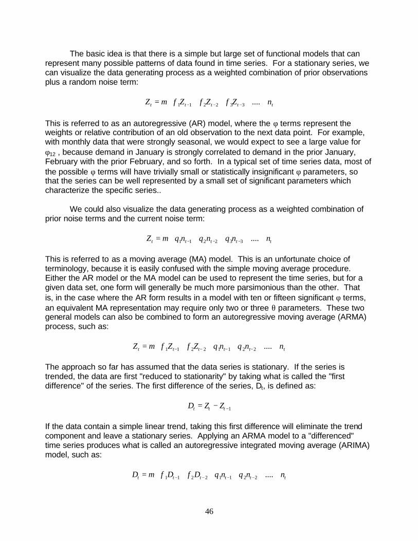
The basic idea is that there is a simple but large set of functional models that can represent many possible patterns of data found in time series. For a stationary series, we can visualize the data generating process as a weighted combination of prior observations plus a random noise term:

Zt = m + f Zt -1 + f Z + f Zt -3 + .... + nt1 2 t -2 3

This is referred to as an autoregressive (AR) model, where the f terms represent the weights or relative contribution of an old observation to the next data point. For example, with monthly data that were strongly seasonal, we would expect to see a large value for f12 , because demand in January is strongly correlated to demand in the prior January, February with the prior February, and so forth. In a typical set of time series data, most of the possible f terms will have trivially small or statistically insignificant f parameters, so that the series can be well represented by a small set of significant parameters which characterize the specific series..

We could also visualize the data generating process as a weighted combination of prior noise terms and the current noise term:

Zt = m + q n + q2nt -2 + q3nt -3 + .... + n1 t -1 t

This is referred to as a moving average (MA) model. This is an unfortunate choice of terminology, because it is easily confused with the simple moving average procedure. Either the AR model or the MA model can be used to represent the time series, but for a given data set, one form will generally be much more parsimonious than the other. That is, in the case where the AR form results in a model with ten or fifteen significant f terms, an equivalent MA representation may require only two or three q parameters. These two general models can also be combined to form an autoregressive moving average (ARMA) process, such as:

Zt = m + f1Zt-1 + f2Zt- 2 + q n +q2nt-2 + .... + nt1 t-1

The approach so far has assumed that the data series is stationary. If the series is trended, the data are first "reduced to stationarity" by taking what is called the "first difference" of the series. The first difference of the series, Dt, is defined as:

Dt = Zt - Zt -1

If the data contain a simple linear trend, taking this first difference will eliminate the trend component and leave a stationary series. Applying an ARMA model to a "differenced" time series produces what is called an autoregressive integrated moving average (ARIMA) model, such as:

Dt = m + f1D + f Dt -2 + q n +q2nt -2 + .... + nt -1 2 1 t -1 t

46

In the identification phase of a Box-Jenkins analysis, an analysis of the correlational structure of the data set is undertaken to determine a parsimonious but adequate model to represent the underlying process. In the estimation phase, non-linear regression tools are used to find specific parameter values (f’s and q’s) that will fit the model to the data with a minimum squared error criterion. Finally, the fitted model can be used to forecast future observations of the series.

The Box-Jenkins approach allows for a rich set of functional forms to model demand data. The analyst uses diagnostic tools such as the autocorrelation functions and partial correlations to interpret the structure of the observations, but the analysis process is complex and requires considerable training and skill. In a system where thousands of individual SKUs must be forecast, the Box-Jenkins approach will likely prove to be too burdensome. The process also requires considerable historical data, and it includes the assumption that the underlying process is time-invariant; that is, that the data generating process does not evolve over time. In studies of actual SKU level demand data, Box-Jenkins forecasts have not generally proven to be more accurate than those generated by simpler tools. For these reasons, Box-Jenkins is not often used for demand forecasting in a logistics system.

Implementation Issues

We have discussed a number of reasonably simple quantitative tools that can be used to develop demand forecasts. In practice, however, this is often the easiest part of the forecasting problem. The forecasting algorithm – the "arithmetic" -- is easily embedded in computer software that is widely available. Many important implementation issues remain, most of which focus on the data being used in the forecasting system. In this section we will focus on a discussion of some of these data issues.

Demand Data Aggregation

Most demand data are composed of many individual elements. For example, store sales are based on customers' individual purchase decisions. These purchase decisions are aggregated in several ways in order to enable managers to use them in decision making. The elemental action is the purchase of a given item by a given customer at a given location on a certain date. The universe of such actions can be aggregated as follows:

Temporally: add up the sales of each product line at each store by day, week, month, quarter and year.

Geographically: add up sales of all departments in a given store, all stores in an area, all areas in a region, all regions in a country, all countries in a continent (or other geographical division used by the firm), and overall total.

By product line: add up all SKU level sales in a sub-category (e.g., soaps) and category (e.g., health and beauty aids).

47

By manufacturer: add up all sales by a given manufacturer.

By socio-economic characteristics: add up all sales by a given customer across all departments and product lines, add up all sales of high-spending customers, etc.

Different aggregations are used for different purposes. In practice, most demand data actually represent several aggregations simultaneously. Thus a material manager may look at a weekly flows of parts from all manufacturers in a certain area of the country into an assembly plant, and a distribution manager may be interested in sales by week or by month at given regions and individual locations, by manufacturer.

It is usually the case that the more aggregated the data, the "easier" it is to forecast. In other words, many forecasts of, say, total annual sales of a given item may be quite accurate; the weekly sales at a given store, however, can be much more difficult to forecast. This is an inherent characteristic of the forecasting process. To see why this is so, consider, a manager who must forecast the daily sales of bottled aspirin at one large drugstore to set orders for deliveries. Suppose we know from past data that the average daily volume is 100 bottles, there is no trend or seasonality in the data, and the standard deviation of demand is ten units, with demand (and hence the noise) normally distributed. Thus the demand data are stationary with L = 100 units and the standard deviation of the noise terms,sn, equal to 10 units. If we forecasted these data using simple exponential smoothing with an a value of 0.2 the long run forecast accuracy would be:

2RMSE = s = 1.05 ·10 = 10.5[a =0.2] 2 - a n

Since these data are stationary, the MAPE should equal 100 times the MAD divided by L:

MAD 2 p RMSEMAPE = = = .0841 = 8.41%

L L

Now suppose we were forecasting weekly sales rather than daily sales. With seven days in a week, expected demand per period would be (7L) or 700 units. Each day has a noise variance of 100 units squared, and the weekly noise variance is (7s2

n) or 700 units squared, so the weekly noise standard deviation is 26.5 units. Thus with an a of 0.20, we would expect an RMSE of 27.9 units and an MAPE of 3.18 %

In general, the standard deviation of the noise terms grows as the square root of the number of periods being aggregated. As a result, the forecast RMSE grows as the square root of the number of periods being aggregated, and the MAPE falls as the inverse of the square root of the number of periods being aggregated. As a rough rule of thumb, for example, if we compared weekly forecasts to monthly forecasts, we would expect the monthly results to have twice the RMSE and half the MAPE.

48

As is illustrated in this analysis, the relative forecast error (MAPE) declines as the aggregation level grows. This is the reason that it may be “easier” to forecast annual sales than daily sales, or regional sales rather than sales at a single store. The effect of aggregation on accuracy can be particularly powerful when the aggregation takes place across SKUs and locations. When the aggregation takes place across time, however, two forces come into play. Notice that in this numerical example the underlying demand process was assumed to be time-invariant. As a result, aggregating demand data reduced relative forecast errors. In many situations, we will face both an "aggregation effect" and a "forecasting horizon effect". In order to aggregate demand over time, we must extend the forecasting horizon. As we have seen, when a demand process is subject to random changes over time, lengthening the forecasting horizon will increase the forecast errors. The extent to which aggregation over time periods will improve forecast accuracy will therefore depend, in each situation, upon which is the more dominant of these two effects. In addition, there will still be the issue of the utility of the forecasts. If the firm really needs weekly forecasts to operate, the fact that monthly or quarterly forecasts may prove to be more accurate is not really relevant.

Sales History versus Demand Data

Most firms believe that they have an extensive historical demand database to use for forecasting, but in fact this is very seldom the case. In most firms, all of these records actually represent sales histories, not demand histories. If the firm enjoys one hundred percent inventory availability, one hundred percent of the time, then this is probably not of great importance. But to the extent that individual items are out of stock, and sales are lost as a result, sales data will generally misrepresent the "true" or "latent" demand that occurred. In many firms, particularly at the retail level, there is no effective way to capture this "missing" demand. In a retail establishment, a customer looks at the shelf, sees the out of stock condition, and buys the item from someone else. Even in the commercial or industrial setting, where it would be possible to capture "lost demand data" in the formal order processing system, very few firms do. As firms move towards increased Supply Chain visibility by allowing their customers one-line, real-time access to their current inventory availability position, more and more commercial and industrial ordering situations begin to resemble the consumer retail shelf in this regard.

As a result, our carefully maintained data may be accurate sales records, but they are not demand data. For purposes of forecasting future demand, we should augment the sales records with estimates of "lost demand", but this is not easy to do. The fundamental question can be thought of as this: How much would we have sold while we were out of stock? Unfortunately, in most cases this is simply "unknowable". On the other hand, if we ignore the issue, then we are implicitly estimating the missing data with a value of zero. Surely we can do better than that.

Suppose, for example, that the record shows that we sold 300 units of an item last month. Suppose the records also show that the item was out of stock for a total of one week last month. If we simply (and conservatively) assume that demand is about the

49

same each day, and that it is not affected by our stock position, then it seems reasonable to estimate that "true demand" was about 400 units. In other words, a very rough way to approximate true demand in a period might be:

Observed Demand"True" Demand =

Fraction of Time In Stock

As simple as this adjustment is, most firms do not use it. There seems to be great reluctance to use "imaginary" data, as opposed to the "real" data in the sales records. The point is, which set of numbers will do the best job of forecasting future demand -- total demand -- for the item? Notice, also, the self-perpetuating nature of this process. We run out of stock in one period and lose some potential sales as a result. Using this sales record, we under-forecast demand in the next period. Based on this low forecast, we carry too little inventory in the next period. As a result, we run out again, and the vicious cycle continues. Eventually, customers tire of our poor inventory availability and they don't come back. At this point our under-forecasts have become a self-fulfilling prophecy. There is no easy analytic solution to this problem. However, it seems clear that for items that have serious availability problems, some adjustment to sales data must be made to correct the biased forecasts that will otherwise inevitably occur.

Demand Displacement

And what about those situations where stockouts do not cause lost sales? In many of these cases, the shortage is addressed by backordering, by shipping from an alternate location, or by item substitution. In these cases, "total demand" is somehow preserved and represented in the firm's sales records, but the records are distorted in a way that will interfere with accurate demand forecasting.

Consider the situation where demand is backordered during stock outages and is satisfied when stock becomes available. For forecasting purposes it is important that the demand is registered as occurring when the property was ordered, not when the order was filled. If we record the sale when filled, the demand is "displaced in time". This distortion or "time shifting" of the data will particularly reduce forecast accuracy when demand is trended or seasonal. If the firm maintains its own backorder records, this is a relatively easy problem to correct. In many cases, however, the customers in effect maintain their own backorders. That is, sometimes loyal customers simply wait until stock is finally available and then buy. In this situation there are no backorder records to work with, but some adjustments are still possible. Suppose we have an item which routinely sells about 100 units per week. We run out of stock, and are out for four weeks. In the fifth week, we sell 500 units. Does this indicate that a large "noise term" happened, or that the demand level on this item has jumped to a new level of about 500 per week, or does this represent "pent up" demand or customer "self-backordering"? How we answer this question will have a significant effect on our forecast -- and our forecast accuracy.

In many logistics systems, an out of stock situation at one location will be handled by satisfying the customer with property from another location. As an example, we might

50

routinely serve a customer in Miami from our regional distribution center in Atlanta. If we are out of stock in Atlanta, and the customer will not accept a backorder, we might ship from our distribution center in Dallas. The shipping will probably cost more, and the transit time will likely be longer, but it is important to fill the orders. Who should receive "credit" for this sale? To keep the on-hand inventory records accurate, we must record the transaction against the inventory in Dallas. For the purposes of demand forecasting, we must record the demand against the Atlanta facility. To do otherwise is to "misplace demand" twice. This would result in exaggerating the demand in Dallas, thus building unnecessary stock, as well as underestimating demand in Atlanta, which would result in under-stocking there.

In still other situations, particularly at the final retail level, temporary stock shortages are handled by item substitution. We wanted to buy a forty-ounce bottle of detergent, but the store was out, so we put a sixty-ounce bottle in our cart instead. We wanted to buy a blue sweater, but our size is sold out. The job of the salesperson at this point is to convince us that we really look good in green, which is available. In each of these situations, demand is almost always recorded against the less preferred alternative, which is the item that was actually sold. Given the use of forecasts to control inventory, the ensuing forecasts will increase the probability that the less preferred item will be available in the next period, and will increase the probability that the more preferred item will not be.

A certain amount of demand displacement seems inevitable in any large inventory system with less than one hundred percent inventory availability. To the extent that it occurs, it will interfere with forecast accuracy. The remedy is conceptually simple: record the demand in the time period, in the location, and against the item where it really occurred. In practice, very few firms have developed the capability to do this.

Treatment of "Spikes" in Demand Data

Sometimes we observe a "spike" in demand; that is, one or two periods of highly unusual demand for an item. Demand might be many multiples above or below its typical level -- far beyond what might be thought of as "just noise" or normal variability. These records may represent errors in the data. Alternatively, the records may accurately reflect what really happened. If the demand was real, management may understand why the unusual demand occurred. Perhaps there was a natural disaster, a weather incident, a major labor strike, or some other dramatic event that caused the disruption of the normal demand pattern. On the other hand, there may be no obvious explanation of why the demand occurred. In any case, how should we treat these data "spikes" when we forecast demand for the item?

Once again, the issue is not whether the demand "really happened"; rather, the issue is whether the use of these data will improve or degrade the forecasts. We know that time series techniques will be influenced by these spikes, and that forecasts in general will move in the direction of the spike. Since spikes do not represent the regular period to period pattern in the data, an ideal forecasting procedure would ignore them.

51

One of the reasons to work with small values for the smoothing coefficients in the exponential smoothing techniques is that small values will not react as strongly to spikes. Another approach is to eliminate the spikes from the demand data and to replace them with more representative data. In a logistics system where thousands of individual SKU level forecasts are being generated, this would be difficult and time-consuming to do manually. It would probably be more reasonable to "filter" the data in the computer program. For example, any demand point that was sufficiently "unusual", say, an observation with a forecast error that is:

| | 4et ‡ · RMSE

might trigger a request for the analyst's intervention, or it might automatically be replaced by a more typical value such as the previously forecasted value for that period.

Another approach to this general problem is to code all sales transactions as they occur as either “recurring demand” or as “non-recurring demand”. Recurring demand is the normal, everyday sales data that we would use to build forecasts. Any sale that was highly unusual or "one time" in nature would be coded as non-recurring demand and would not be used for forecasting. This approach has been used for decades in the military logistics systems of the United States. For example, a fighter aircraft traveling cross-country might need to stop at a bomber base for unscheduled repairs. Any spare parts that were needed would be ordered and coded as non-recurring demand so that the forecasting and inventory algorithms would not begin to routinely stock the fighter parts at the bomber base.

The emphasis throughout this chapter has been on formal statistical forecasting methods. These methods draw information out of data that are assumed to be based on simple underlying patterns and random process. In many cases, however, a significant effort should be spent before any forecasting model is developed to extract a deterministic part of the observation. Many data patterns include orders or shipments based on MRP systems, accounting practices, incentive pay of various actors in the supply chain, national holidays around the globe, or other planned or predictable events.

Frequently such sources generate lumpy demand with distinct patterns. Separating this demand from the rest allows different treatment of this demand. For example, in the context of supplying an assembly plant, major parts and sub-assemblies that are particular to specific products should be treated deterministically, since they can be derived directly from the production schedule. Such inbound parts could be ordered and supplied “just-in-time ‘ to minimize inventory build up. Less expensive items, as well as parts and material which are used in many products, should be forecasted using statistical methods since the demand for them is the result of the demand for many different products, each of which may be facing changing final demand conditions.

52

Demand for New Items

New product introductions present a special problem in that there is no historical time series available for estimating a model. At issue is not only the estimation of the sales at every future period but also, for example, estimates of the time it takes to reach certain sales volumes.

In this and other contexts where there is no reliable historical time series or when there are reasons to believe that future patterns will be very different from historical ones, qualitative methods and judgment are used. Unfortunately, many market research procedures, which are based on questionnaires and interviews of potential customers, notoriously over-estimate the demand since most respondents have no stake in the outcome. Data can also be collected from marketing and sales personnel, who are in touch with customers and can have an intuition regarding the demand for some products. Other sources of informed opinions are channel partners, such as distributors, retailers, and direct sales organizations.

The growth rates of similar products may also provide some guidelines, particularly, if the analysis is coupled with comparative analyses of each of the other products' attributes, the market conditions at product launch, and the competitive products at the time. All of these factors should be contrasted with the product being launched in the current environment, and a composite forecast should be developed based on the weighted sales rates of past products.

Among the formal methods, causal models play a special role in cases where a historical time series is not available. Disaggregate demand models can be used to formally capture the probability of purchase given a set of product attributes and the characteristics of the target population. Collecting disaggregate data is, however, expensive and the analysis requires some expertise. Alternatively, multiple regression models can be used to analyze the initial sale patterns of other products, which can be characterized by their attributes and the population's characteristics. The new product attributes are then applied using the estimated parameters.

Any formal time series procedure can only be used after a few observations become available. The parameters of such a forecasting model should be "aggressive", that is, using only a few observations in a moving average, or a high value of the smoothing constant in a simple exponential smoothing model. Once more information becomes available these parameters can be re-set to a typical value.

Collaborative Forecasting

Many firms have moved beyond the integration of their internal logistics processes and decision-making and have begun to focus on the close integration of logistics processes with their trading partners both backwards and forwards in the distribution channel. This inter-organizational logistics focus has come to be called Supply Chain Management. In Supply Chain Management, firms attempt to improve the efficiency of

53

their logistics efforts through joint, cooperative efforts to manage the flow of goods in a "seamless", organic way throughout the channel. Each firm attempts to share useful data and to coordinate all important logistics decisions. One logistics process that could benefit dramatically from this kind of cooperation is demand forecasting. Many firms are now working on cooperative forecasting techniques, and this general idea has come to be called collaborative forecasting.

Consider the traditional distribution system relationships between the manufacturer of a consumer packaged good and the retailers who sell the product to the public. Each retailer must forecast demand for each SKU at the store level. Based on these forecasts and on a consideration of available inventory, warehouse stocks, lead times, promotion plans, and other factors, each retailer than develops an "order plan" which contains the timing and size of the stock replenishment orders that the retailer intends to place on the manufacturer. While this is going on, the manufacturer is also forecasting its demand for each item by time period. In effect, the manufacturer is trying to forecast, time period by time period, the effective sum of the order plans from all of the retailers. In traditional practice, the manufacturer forecasts this total demand independently, with no input from the retailers. In collaborative forecasting, the retailers would share their demand forecasts and their current order plans with the manufacturer, and the manufacturer would aggregate these data to construct and verify its forecasts. Discrepancies between the retail order plans and the manufacturer forecasts would be identified and resolved. The final result would be improved forecast accuracy, less total inventory in the system, and a smoother deployment of the goods into the retail channel.

The central premise of collaborative forecasting has great merit, but there are a number of potential problems that must be solved to gain the promised benefits. First, there is an issue with the level of aggregation of the forecasts being shared. Second, there is a communications issue involving the transfer of these data between firms. Finally, there is an issue with the sheer volume of data that would be processed in such a system.

The first issue is that of aggregation. While the retailer plans orders that represent demand or replenishment to its stores, the manufacturer often forecasts its demand in total. Suppose, for example, that a retailer shared with us that it planned to order 100,000 units during a coming period. As the manufacturer, our prior forecast of our total demand for that same period was, let us say, 1,000,000 units. What would we do with this new, and presumably more accurate, information? Our previous estimate of this one retailer's probable order is somehow included in our total forecast, but this retailer's contribution to the total is not explicit due to the aggregation. For the collaboration strategy to be useful, the manufacturer must forecast demand at the level of the individual retailer, rather than at the level of total demand. If the manufacturer sells through a channel that consists of thousands of small independent retailers this will not be practical. However, suppose the retail level of the channel can be thought of as : (1.) WalMart, (2.) KMart, (3.) Target, and (4.) all other retailers. Given the ongoing concentration in the mass merchandizing sector of retailing, these four demand segments might have roughly equal sales volumes. By forecasting demand at the level of these major segments, the manufacturer gains the ability to work with shared data from major trading partners. In practice, many

54

manufacturers are already forecasting demand at the level of their major retail customers because of the importance of these channel partners.

The second implementation issue is that of data transmission. A collaborative forecasting scheme would involve passing large volumes of data between many firms. Common data standards will be essential to the success and widespread adoption of these tools. In 1998 the VICS (Voluntary Interindustry Commerce Standards) organization issued the "Collaborative Planning, Forecasting, and Replenishment (CPFR) Voluntary Guidelines". This document outlines a vision for implementing collaborative forecasting through the use of standard EDI transaction sets and commonly agreed upon business practices. To quote from the VICS guidelines:

"How does CPFR work? It begins with an agreement between trading partners to develop a market specific plan based on sound category management principles. A key to success is that both partners agree to own the process and the plan. This plan fundamentally describes what is going to be sold, how it will be merchandised and promoted, in what marketplace, and during what time frame. This plan becomes operational through each company's existing systems but is accessible by either party via existing VICS-approved communications standards.

Either party can adjust the plan within established parameters. Changes outside of the parameters require approval of the other party, which may require negotiations. The plan becomes the critical input to the forecast. The CPFR plans are rolled up, and the balance of the forecast (for non-CPFR participants) is arrived at through forecasting models.

With CPFR, a forecast can become frozen in advance, and can be converted automatically into a shipping plan, avoiding the customary order processing which takes place today. CPFR systems also capture mission-critical information such as promotion timing and supply constraints that can eliminate days of inventory from the entire supply chain and avoid meaningless exception processing."

Working within the framework of agreed upon data transmission standards should greatly simplify the problem of implementing a collaborative forecasting relationship, but there still remains the very serious problem of processing the enormous volume of data implied by the collaboration. Most firms have developed forecasting systems and software that focus on the problem from the perspective of the individual firm, working with one large set of forecasts. In a collaborative scheme, the emphasis shifts to the comparison and collation of alternative forecasts of the same demand activity as predicted by different channel partners. Analytic capability is needed to search for meaningful similarities and differences in the data being shared. Whole new classes of software are being developed to provide this capability. For example, Syncra Software, Inc. has developed tools that it describes as "BetweenWare" because these tools focus solely on trading partnerships and cross-functional relationships. While recognizing that common data transmission standards are an essent ial first step, Syncra suggests that the larger problem remains:

55

"....And therein, as is common with all industry standards, is the problem. While the standards describing and enabling the exchange of business transaction data are quite clear, it is usually people, not systems that resolve supply chain tension. The issues arising from the lack of a common 'view' to the information and the ability to filter 'actionable requirements' from among the billions of bits of data among the participants in a supply chain result in a daunting barrier to a widely deployable and implementable solution that can achieve 'critical mass' ".

The software produced by Syncra and other firms are attempts to provide the firm with the data processing capabilities they will need to fully exploit the potential of the collaborative forecasting concept.

56