Naval Research LaboratoryWashington, DC 20375-5320

NRL/MR/7100--15-9602

Mode 2 Internal Wave Generation andPropagation Near the New Jersey (USA)Shelf Break–Early Fall Season

March 13, 2015

Approved for public release; distribution is unlimited.

Marshall h. Orr

The University of DelawareNewark, Delaware

ThOMas E. Evans

Coastal and Ocean Remote Sensing BranchRemote Sensing Division

i

REPORT DOCUMENTATION PAGE Form ApprovedOMB No. 0704-0188

3. DATES COVERED (From - To)

Standard Form 298 (Rev. 8-98)Prescribed by ANSI Std. Z39.18

Public reporting burden for this collection of information is estimated to average 1 hour per response, including the time for reviewing instructions, searching existing data sources, gathering and maintaining the data needed, and completing and reviewing this collection of information. Send comments regarding this burden estimate or any other aspect of this collection of information, including suggestions for reducing this burden to Department of Defense, Washington Headquarters Services, Directorate for Information Operations and Reports (0704-0188), 1215 Jefferson Davis Highway, Suite 1204, Arlington, VA 22202-4302. Respondents should be aware that notwithstanding any other provision of law, no person shall be subject to any penalty for failing to comply with a collection of information if it does not display a currently valid OMB control number. PLEASE DO NOT RETURN YOUR FORM TO THE ABOVE ADDRESS.

5a. CONTRACT NUMBER

5b. GRANT NUMBER

5c. PROGRAM ELEMENT NUMBER

5d. PROJECT NUMBER

5e. TASK NUMBER

5f. WORK UNIT NUMBER

2. REPORT TYPE1. REPORT DATE (DD-MM-YYYY)

4. TITLE AND SUBTITLE

6. AUTHOR(S)

8. PERFORMING ORGANIZATION REPORT NUMBER

7. PERFORMING ORGANIZATION NAME(S) AND ADDRESS(ES)

10. SPONSOR / MONITOR’S ACRONYM(S)9. SPONSORING / MONITORING AGENCY NAME(S) AND ADDRESS(ES)

11. SPONSOR / MONITOR’S REPORT NUMBER(S)

12. DISTRIBUTION / AVAILABILITY STATEMENT

13. SUPPLEMENTARY NOTES

14. ABSTRACT

15. SUBJECT TERMS

16. SECURITY CLASSIFICATION OF:

a. REPORT

19a. NAME OF RESPONSIBLE PERSON

19b. TELEPHONE NUMBER (include areacode)

b. ABSTRACT c. THIS PAGE

18. NUMBEROF PAGES

17. LIMITATIONOF ABSTRACT

Mode 2 Internal Wave Generation and Propagation Near the New Jersey (USA)Shelf Break–Early Fall Season

Marshall H. Orr1 and Thomas E. Evans

Naval Research Laboratory, Code 71004555 Overlook Avenue, SWWashington, DC 20375-5350

NRL/MR/7100--15-9602

UW-435-27

Approved for public release; distribution is unlimited.

1The University of Delaware, The College of Earth, Ocean and Environment, 111 Robinson Hall, Newark, DE 19716. The research reported here was performed while the author was employed in the Acoustics Division, Naval Research Laboratory.

UnclassifiedUnlimited

UnclassifiedUnlimited

UnclassifiedUnlimited

UnclassifiedUnlimited

41

Douglas G. Todoroff

(202) 767-3482

Mode 2 internal waves have been repeatedly observed in two separate bathymetry zones on the New Jersey (USA) continental shelf. In the first zone, the upslope propagating mode 2 internal waves were detected in a ~15 km range interval shoreward of the shelf break in water depths ranging between ~90 and 150 m. They were formed in conjunction with shoreward propagating internal tides and exhibited both nonlinear and linear characteristics. In the second zone, they were detected in 60 to 80 m water depths and appeared to be formed by flow over the local bathymetry. Simulations using the Shen Non-hydrostatic Model for Coastal Oceans (SNMCO) replicated the observed coupled internal tide and mode 2 internal wave generation process and separately the formation of mode 2 internal waves by flow over local bathymetry variability. The observations expand the knowledge base regarding the time window (fall, 7 days before and including neap tidal conditions), spatial distributions, packet evolution and conditions under which mode 2 internal waves are generated on the continental shelf.

13-03-2015 Memorandum Report

Continental shelfMode 2 internal wave generation and propagationRelation to internal tide

October 2011 – September 2013

6534

Naval Research Laboratory, Code 71004555 Overlook Avenue, SWWashington, DC 20375-5350

1

1. Introduction

Second baroclinic mode internal waves (mode 2 internal waves) are being detected with

increasing frequency in stratified continental slope, shelf and deeper waters. Recent papers and

publications include those of Bogucki, Redkopp and Barth [2005], Henyey, Williams, Becker,

Lyons, Ballard, Camin, Gabel, Koszalka and Beitel [2006], Orr [2004], Yang, Fang, Chang,

Ramp, Kao, and Tang [2009], Smith, Bradley, Mignerey and Goldstein [2009], and Shroyer,

Moum and Nash [2010].

Yang et al.[2009] and Shroyer et al.[2010] have provided detailed references and summaries

describing the theory, laboratory experiments and field observations related to mode 2 internal

wave generation and propagation.

In overview, mode 2 internal wave generation and propagation has been studied in the laboratory

by Davis and Acrivos [1967a], Helfrich and Melville [1986] and Mehta, Sutherland and Kyba

[2002]. The topic has been treated theoretically and numerically by a number of authors

including Davis and Acrivos [1967a and 1967b], Yih [1960, 1961], Benjamin [1967], and Stastna

and Peltier [2005].

Davis and Acrivos [1967a] performed laboratory experiments using a tank in which two fluids of

equal thickness but differing density were separated by a thin continuous gradient. Injection of a

fluid (gravity flow-like) at the depth of the gradient caused the formation of mode 2 interfacial

waves. Unlike mode 1 internal waves which displace the top and bottom of the pycnoline in

phase, a mode 2 internal wave displaces the top and bottom of a pycnocline 180 degrees out of

phase. When the interfacial mode 2 waves were of large amplitude compared to wavelength,

closed streamline flow was observed and the waves were considered to be nonlinear, see Davis

and Acrivos [1967a] Figure 5. When the interfacial waves were of small amplitude compared to

wavelength, closed streamline flow was not observed and the waves were assumed to be weakly

nonlinear or linear in nature. Mehta, Sutherland, and Kyba [2002] have studied the response of

two and three layer salt stratified fluids to interfacial gravity currents, and have observed the

formation of double-humped solitary waves. In addition, Vlasenko and Hutter [2001] have

demonstrated in the laboratory the generation of mode 2 internal waves during the passage of

mode 1 internal waves over sills. They developed a numerical model that replicated their

observations.

Nonlinear mode 2 internal waves were observed in the vicinity of the USA New Jersey shelf

break during August of 2006 by Shroyer, et al. [2010]. The density profile consisted of a ~10 m

shallow mixed layer, a ~ 5 m pycnocline and a nearly iso-density layer to the shelf bottom. The

mode-2 internal waves which were located in the pycnocline were detected with a ship borne 120

kHz acoustic backscattering system, moored vertical temperature arrays and bottomed acoustic

Doppler current profilers. A mode 2 internal wave group named Jasmine was observed to evolve

______________________________________________________________

Manuscript Approved September 29, 2014

2

over time by radiating short wavelength mode 1 internal waves when the propagation speeds of

the mode 1 and mode 2 internal waves were equal. The energy loss during the mode 2 to mode 1

wave conversion was estimated. The mode 2 internal wave group generation site, generation

mechanisms and propagation lifetimes were not identified. The authors proposed that the mode

2 waves could be formed by either tidal forcing near the shelf break or frontal intrusions which

are known to occur in the area. Their shipboard mode 2 internal wave observations were in the ~

90 to 110 m depth interval, see black triangles, Figure 1. Three moorings were located

shoreward and one was located seaward of the shipboard observations. All are noted with black

diamonds. Nonlinear mode 2 internal waves were detected at the two moorings near 39 N and -

73.1 W. No nonlinear mode 2 internal waves were detected at the 39.08 N and -73.19 W

mooring or the mooring near the shelf break. Mode 2 waves were detected at another mooring

that was located 20 km shoreward of the moorings near 39 N and -73.1 W.

This manuscript describes mode 2 internal wave groups that were imaged with a 200 kHz

acoustic backscattering system near the New Jersey (USA) shelf break. The data was taken in

early fall when the mixed layer was near half water column depth. Analysis of the data has

resulted in: 1. the identification of two bathymetry zones where the mode 2 internal waves were

generated; 2. the identification of two mode 2 internal wave generation processes; 3. the

characterization of the spatial evolution of mode 2 internal wave groups generated near the

continental shelf break; and 4. the identification of mode 2 internal waves with nonlinear and

weak nonlinear characteristics similar to those created in the laboratory by Davis and Acrivos

[1967a] and observed by Shroyer et al. [2010]. One generation zone was located in a 15 km

range interval shoreward of the shelf break in water ranging from 90 to 150 m in depth. The

second was located in water depths ranging from 60 to 80 m in the immediate vicinity of

bathymetry variability (sills).

In the following sections the experimental measurements are outlined and the observations are

presented and related to acoustic Doppler current profiler, pressure gage, and temperature and

salinity vs. depth and range measurements. Numerical simulations which replicate aspects of the

of the two observed mode 2 internal wave generation processes are overviewed and future

studies to quantitatively access the impact of mode 2 internal waves on the kinematics and

dynamics of the shelf waters are discussed.

2. Experiment

The observations were made near the United States of America’s New Jersey shelf break, see the

Google Earth insert in Figure 1. A shipboard sensor suite on the Research Vessel (R/V)

Endeavor and bottom moored acoustic Doppler current profilers (ADCP) were used to measure

the temporal and spatial variability of the temperature, salinity, density and current fields. A

pressure gauge was deployed near one of the ADCP moorings. The experiment was conducted

from 27 September to 4 October 2000. In geotime this corresponds to Yearday 271 to Yearday

278 where Yearday 1was defined as 0000 – 2400 GMT, Jan 1, 2000.

The components of the shipboard instrument suite pertinent to the observations and data

interpretation included a ScanFish; a rosette, radars; an ADCP; and a Naval Research Laboratory

(NRL) 200 kHz nadir incident high frequency acoustic flow visualization (HFFV) system. The

3

ScanFish and rosette were both instrumented with SeaBird 9 Plus profiling conductivity,

temperature and depth measurement systems (CTD) which acquired data at a 24 Hz sample rate.

The radars, a Sperry Marine Equipment Rascar 2500 25 KWX and a 50 KWX Model # 1D-

251C-1, were used to detect the surface expression of internal waves. Signals from the

shipboard radar systems were recorded during the experiment period.

The ScanFish was towed at speeds ranging from ~ 3 to 3.5 m/s and cycled from ~5 to 10 m

below the surface to ~ 10 m above the bottom every ~ 3 to 4.5 min depending on water depth.

Due to the cycle intervals, internal waves at mid-water depth were not adequately spatially

sampled when their wavelengths were smaller than ~ 1800 m. The ship made 84 transects of

varying length over sections of a northwest/southeast oriented (309o/129

o) cross-shelf track and a

northeast/southwest oriented (56o/236

o) along-shelf track, see solid white lines plotted on Figure

1. The cross-shelf track was oriented parallel to the known internal tide and associated mode 1

internal wave group propagation direction, Apel et al. [1997]. The ScanFish CTD measurements

were used to: 1. characterize the larger scale (> 1 km) temporal and spatial variability of the

temperature, salinity and density fields; 2. corroborate the interpretation of the high frequency

acoustic flow visualization (HFFV) data; and 3. provide the temperature and salinity

initialization fields used in the Shen Non-hydrostatic Model of Coastal Ocean (SNMCO)

numerical simulations to be presented later.

In addition to the ScanFish transects, the R/V Endeavor also made occasional vertical rosette

casts while drifting and continuous casts while moored during a ~18.6 hour interval from

Yearday 277.9035 to Yearday 278.6778 GMT. The mooring point was near 39.3454 N and -

72.8822 W and is marked on Figure 1 with a red bordered triangle above arrow 1. A total of 160

casts were made. The water depth was ~ 70 m and the winch rate was 30 m/min resulting in a

cycle time of about 4.6 min. Consequently, the yo-yo CTD measurements were temporally

aliased for internal waves with periods less than about 11.5 min.

The NRL high frequency (200 kHz) acoustic flow visualization system (HFFV) continuously

imaged fluid processes at smaller spatial or temporal scales than could be sampled with either the

ScanFish or the rosette. Consequently, it was the primary instrument used to detect the mode 2

internal waves observed during this experiment. Depending on water depth the HFFV

transmitted a 10 cycle sine wave signal two or four times per second. The system had a vertical

resolution of ~ 0.0375 m and at a range of 100 m had a horizontal resolution of ~ 1.7 m at the 3

dB down points of the main lobe of the transducer beam pattern. At a ship speed of 3.5 m/s,

acoustic signals scattered from impedance variability at ranges up to 100 m were received within

the primary lobe of the beam pattern and used to image the vertical displacement of the water

column. The impedance variability can be caused by particles (biology or detritus) or separately

temperature, salinity or velocity fluctuations. When the impedance variability is neutrally

buoyant in the fluid, it acts as a Lagrangian tracer and permits the imagery of a variety of fluid

processes including front movement, internal wave displacement of the pycnocline, shear

instabilities and turbulent mixing e.g. Farmer and Smith [1980], Goodman [1990], Stanton et al.

[1994] and Orr and Hess [1978]. An illustrative HFFV image, Figure 3b ii, shows scattering

from the ocean bottom (~ 60 to 140m) and the top of the pycnocline. The zero range point for all

cross-shelf HFFV images and ScanFish plots presented in the following sections is noted by a

white diamond (39.4813 N; -73.1250 W) located at the northwestern end of the cross-shelf

4

transect line, see Figure 1. The bathymetry plotted in the Figure 1 is from the National

Oceanographic and Atmospheric Administration (NOAA) National Geophysical Data Center

U.S. Coastal Relief Model.

Two bottom mounted RD Instruments 307.2 kHz broadband ‘Workhorse Sentinels’ ADCPs were

placed close to the cross shelf transect line and are marked in Figure 1 with white diamonds

overlain with red asterisks and in Figure 3 and subsequent image figures with white triangles.

This article will focus on the ADCP 2 measurements, e.g. Figure 2a and b. It was moored in ~

118.6 m of water near the 45 km range point of the cross-shelf transect line and measured

currents in two meter steps in the 14.9 to 116.9 m depth interval by acquiring 120 pings in one

minute bursts every 4 minutes. In the following discussions the current data will be related to

the HFFV data. An analysis of the ADCP measurements found that the 0.5 – 7.5 cycles per hour

internal wave frequency band was dominated by mode 1 internal waves, Hallock and Field

[2005].

A pressure gauge mooring was located ~ 4.22 km to the northwest of ADCP 2. Its

measurements are plotted with the ADCP 2 current data, e.g. Figure 2c.

3. Observations

Two consecutive days were spent making ~ 30 to 45 km cross-shelf transects along portions of

the white line between the white triangle near the shelf break and the white diamond near 39.48

N and -73.1250 W. Several days were spent acquiring ~12 km cross-shelf and along-shelf

transects between the solid white circles in the ~ 90 to 150 m depth range, see Figure 1. Mode 2

internal waves and groups were intercepted 83 times during the transects. The waves were

propagating shoreward with a water referenced speed of ~ 0.2 m/s. The location of some of the

mode 2 internal wave detections are plotted as black squares, see Figure 1. Some of the mode 2

detection locations along the cross-shelf transect line are marked with red Xs along the 5 m depth

line in the Figures 3 and several subsequent figures. As can be seen, the majority of the cross-

shelf mode 2 internal wave detections were in the ~90 to 150 m depth range in a ~15 km range

interval shoreward of the shelf break and seaward of the increase in the bathymetric slope near

the 43 km range point. The large number of detections in the depth range is weighted by the

amount of survey time spent in that range as noted above. On occasion, during the transects

shoreward of the 15 km range interval and when the R/V was moored, mode 2 internal waves

were detected in 50 to 80 m of water in the vicinity of local bathymetry variability (sills), see

arrows 1 and 2 in Figure 1.

The HFFV observations of the mode 2 internal wave generation, propagation and evolution will

be described and related to the ScanFish CTD, the ADCP 2 current and the pressure gauge

measurements. First each of the measurement types will be characterized.

A section (Yearday 272.8 to ~ 273.3) of the ADCP 2 data shows the current parallel to and

perpendicular to the cross-shelf transect line as well as the pressure gauge measurement, see

Figure 2a, b and c respectively. The current oriented parallel to the transect line shows phase

coupling to the barotropic tide, the presence of vertical shear and a 5 to 10 m thick offshore

current jet in the 30 to 40 m depth interval (see above the black arrows in Figure 2a). The

offshore current jet persisted during onshore flow periods. The along-shelf current, Figure 2b,

was predominately to the southwest with limited periods of northeast flow. This time section

5

shows one of the few northeast flow events in the Yearday 273.4 to 273.6 time interval. Based

on the ADCP 2 current record two assumptions were made concerning the interpretation of the

HFFV images to be presented below. The first was that flow induced pycnocline depth

variability is caused by current flowing parallel to the transect line and over the in-plane

bathymetry variability. The second was that no out of plane bathymetry variability oriented

parallel to the cross-shelf transect line complicated the imaged in-plane fluid dynamics. The

latter assumption appears justified because the along-shelf bathymetry variability northeast of the

transect line in the 90 to 150 m depth range is limited, see Figure 1. These assumptions do not

preclude pycnocline displacement by internal tides and associated internal wave groups.

A ScanFish temperature and salinity field measurement along a ~ 45 km section of the cross-

shelf transect line (YD 272.4728 to 272.6451) illustrates the complexity (> ~2 km scale) of the

water column and the variability in the underlying bathymetry (black line), see Figure 3a. The

water column was composed of interleaving water masses with differing salinity and temperature

composition, e.g. see above arrow 1 and arrow 2 in Figure 3a i and ii. During subsequent

transects the individual water masses were observed to be displaced up and down slope by the

cross-shelf current. Some of the water mass variability was also expected to be caused by along-

shelf transport through the transect path. The ScanFish data was taken a few hours before the

deployment of the ADCP 2 and the nearby pressure gauge. Back projection from the pressure

gauge measurements indicates high tide and minimum on-shore current flow occurred near the

midpoint of the transect time interval. Internal wave displacements of the pycnocline are seen in

both the temperature and salinity records, e.g. near bathymetry variability at the ~ 16 km and 25

km range points, e.g. the arrow 3 and 4, Figure 3a i.

The density field derived from the above measurements and a HFFV image acquired in

time/space coincidence with the ScanFish data, Figure 3b i and ii respectively, both show the

same ~ 2 km and longer wavelength mode 1 internal wave displacement of the pycnocline, e.g.

arrows 1 and 5. There were two internal tides present, see the horizontal blue arrows in the 24 to

35 km and ~ 42 to 55 km range interval in Figure 3b i. A lens of light water occupies the 20 to

30 m depth interval in the ~ 10 to 30 km range interval. The same internal tide structure is seen

to the right of arrow 2 and 5 in the HFFV image. Enlargements of the HFFV image (not shown

due to space limitations) revealed short wavelength mode 1 internal waves of ~10 m amplitude

and ~ 400 m wavelength near the front of the internal tide, above arrow 2 Figure 3b ii. In

addition, 2 to3 meter amplitude mode 2 internal waves were imaged in the 30.5 to 33.5 km range

interval, above arrow 3, and in the 45 to 46 km range interval, above arrow 4. Both of the

imaged internal tides had a mode 2 internal wave structure associated with them. The density of

the water decreased from the shelf break area, near 53 km, shoreward, Figure 3b i. The range

dependence of the density structure was more complicated than the range independent two layer

fluid structure used in the mode 2 internal wave laboratory measurements mentioned earlier, e.g.

Davis and Acrivos [1967a]. However, the density field did approximate a two layer fluid of

equal thickness separated by a pycnocline. During the field observations both the vertical

gradient of the pycnocline and the average density which decreased in shoreward direction were

range dependent. In summary, near high tide mode 2 internal waves were detected downslope

from the leading edge of two upslope propagating internal tides. The HFFV image provided

detailed spatial information about the vertical displacement of the pycnocline by both mode 1

and mode 2 internal waves. It also replicated the long wavelength pycnocline displacements

6

seen in the density field data. Due to the pixel resolution limits of printed media and the ~ 10 m

to 30 km length scales of the fluid processes to be discussed, the HFFV images that are presented

will range from 20 to 40 km in length sections, as done for Figure 3b ii to illustrate the

interrelationship of internal tide and the generation of mode 1 and mode 2 internal waves to

enlarged sections that show the 1 to 5 km length scales relevant to the mode 2 internal wave

groups’ propagation and evolution.

Representative fall, mid-summer and late fall density and buoyancy frequency profiles for the

New Jersey shelf are plotted in Figure 4a and b. The seasonal evolution of the pycnocline and

the buoyancy frequency profiles stands out. The fall density field approximated a two layer fluid

of equal thickness with a pycnocline separating the layers. This density profile is similar to that

used in the above mentioned laboratory studies of mode 2 internal wave generation and evolution

and in theoretical treatments. As noted in the previous paragraph and will be expanded on in the

following paragraphs, mode 2 internal waves were imaged in the fall density profile. However,

Shroyer et. al [2010] have also imaged mode 2 internal wave groups in a summer density profile

similar to that shown in this figure. The separate observations in two distinct density profiles is

interesting and suggests the impact of density structure variability on the formation and

propagation of mode 2 internal waves will need to be addressed. The summer density data was

acquired in late July early August 1995, Apel et.al. [1997] north of the Shroyer et. al [2010]

experiment site and southwest of the transect line shown in Figure 1. The late fall data was

acquired during a NRL experiment at the same location.

Cross-shelf HFFV Transect Observations

Three HFFV image sets which show the generation, propagation and temporal/spatial evolution

of mode 2 internal wave groups in the 90 to 150 m depth interval are presented below. The first

set is for a 19.75 hour time interval, the second spans a 5.74 hour interval and the last is a 1.47

hour long observation.

First Illustration

The first set of images was acquired during six consecutive upslope and downslope transects.

The phase of the tide and the current measured at ADCP 2 during each transect are shown in

Figure 2. The transect numbers and intervals are labeled below the abscissa. The vertical dash

dot black lines show the start time of a transect, the dashed vertical red lines indicate the transect

stop time. The alternate black red vertical lines indicate that the termination of one transect and

the start of the next transect were close in time. The times that the R/V passed the ADCP 2 are

noted by the solid vertical magenta lines. In Figure 2a positive current is offshore along the

cross shelf transect line and in Figure 2b positive current flows in the ~39 degrees east of north

direction.

The ~30 km long HFFV image in Figure 5a was acquired during the upslope transect 1 (Yearday

273.1948 to 273.3261). It shows the displacement of the pycnocline as the outflowing current at

ADCP 2 transitioned from near max offshore to the initiation of onshore flow following low tide,

see Figure 2 transect 1. The image in Figure 5b was acquired during the downslope transect 2

(Yearday 273.3261 to 273.4660). It shows the displacement of the pycnocline as the tidal flow

7

at ADCP 2 accelerated to maximum onshore flow near the middle of the transect interval, see

Figure 2 transect 2. In both cases current shear was present. The two transects were acquired

during a ~ 6.5 hour time interval. ADCP 2 was located near the 45 km range point, see the white

triangle. It is important to note that the HFFV images are not in a coordinate system that

provides a snapshot of the pycnocline displacement at a time instant for all space but are in a

coordinate system where the pycnocline displacement measured at each range point has evolved

during the time interval it takes the research vessel to move to that point from a previous point.

For instance, in the upslope transect, Figure 5a, the portion of the image near arrow 4 was taken

when flow at ADCP 2 was near max offshore while the portion of the image at arrow 2 was

taken when flow at ADCP 2 was near slack. Interpretation of the images must take the

coordinate system time delay into account. Due to the propagation speed of the internal tide and

its associated internal waves, the closer in space that imaged events of interest occur the closer in

time coincidence the events are from a fluid dynamics perspective.

Near maximum offshore flow the upslope transect 1 image, Figure 5a, shows a small amplitude

(3-5 m) mode 1 internal wave group in the 52 km range interval above arrow 3 and a hydraulic

feature with mode 2 characteristics in the 53 to 54 km range interval above arrow 4. Near

maximum onshore flow conditions the reciprocal downslope transect 2, detected a ~ 15 m

amplitude mode 1 internal wave group at the leading edge of the next internal tide near 47 km,

see arrow 3 Figure 5b, and a hydraulic feature with mode 2 characteristics near the 52 km range

point, arrow 4. The mode 1 internal wave was generated during the 5 hour interval between the

upslope transect 1 and the downslope transect 2 intercept of the 48 km range point. The

scattering feature with mode 2 characteristics between the arrows 7 and 8 was caused by a lens

of warm saline water and is not considered to be a mode 2 internal wave.

During both transects upslope propagating mode 1 internal waves at the leading edge of an

internal tide were imaged in the ~70 to 80 m depth interval, see arrows 1 and 2 in Figure 5a and

5b. The ScanFish derived density field, not shown but similar to Figure 3b i in character, also

indicated that the mode 1 internal waves were associated with the internal tide. The time interval

between the internal wave intercepts, see arrow 2 in Figures 5a and 5b, was 1.816 hours. The

over ground upslope propagation speed for the internal wave was ~ 0.53 m/s. The upslope

current was ~ 0.05 m/s. Note the spatial separation between the internal wave at arrow 2 in

Figure 5b and the mode 1 internal wave at arrow 3 in Figure 5b is about 18 km. This is the

distance an internal tide and associated mode 1 internal waves will propagate in ~ 12 hours with

an average over the ground speed of 0.42 m/s. Consequently, it is reasonable to assume that the

internal tide and mode 1 internal waves at arrow 1 and 2 were generated during the previous tidal

cycle in the same region as the mode 1 internal wave group imaged at 48 km, arrow 3, in Figure

5b.

Although thickening of the pycnocline, suggesting mode 2 pycnocline displacement was present

in the vicinity of arrow 5 in Figure 5a, enlargement of the image revealed no distinct mode 2

internal wave structures. In the 5 hour time interval between the upslope transect 1 and the

downslope transect 2 intercept of the 48 km range point two distinct mode 2 internal wave

groups formed between the 39.5 and 45.7 km range points, see Figure 5b, arrow 5 and 6.

Enlargements of the mode 2 internal wave groups above arrow 5and 6 are presented in Figure 6a

and b, respectively. The mode 2 internal wave group near 39.5 km was about 1.1 km in length,

8

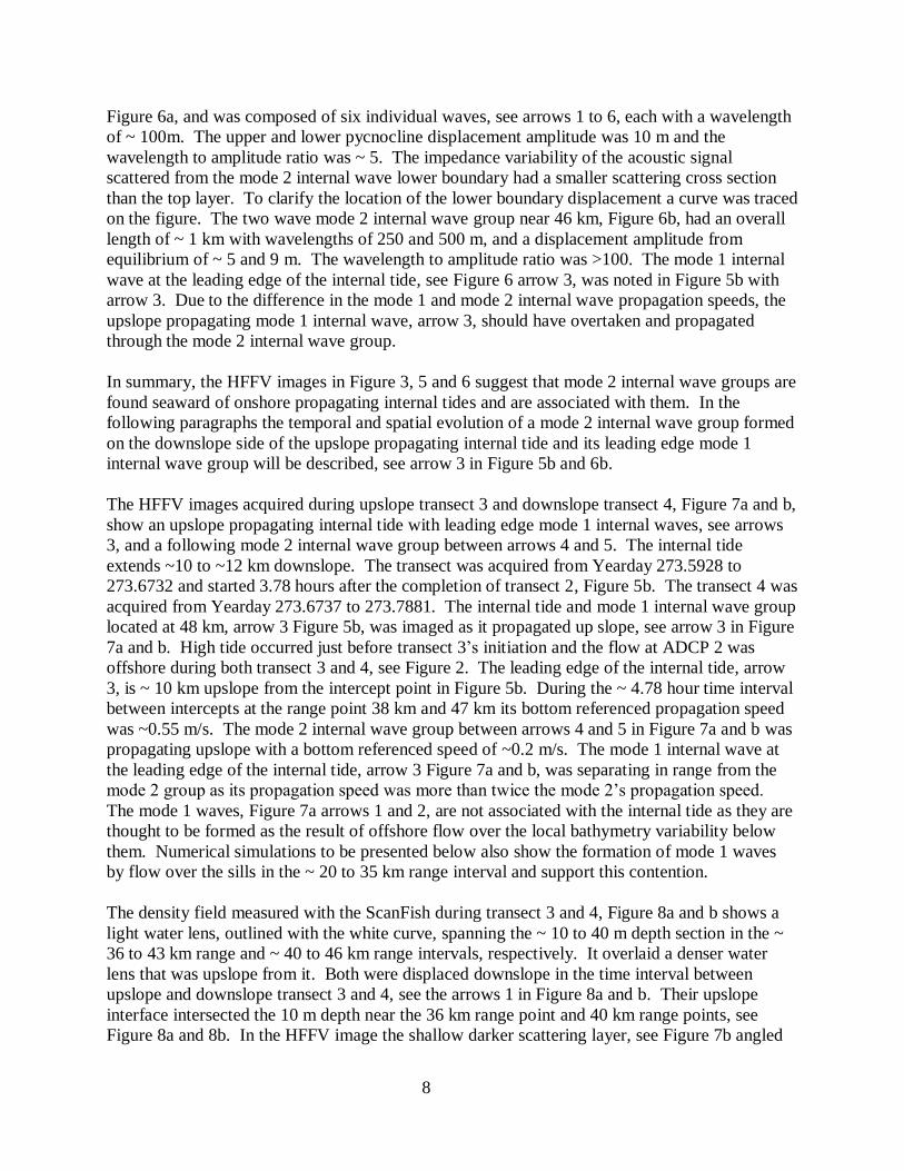
Figure 6a, and was composed of six individual waves, see arrows 1 to 6, each with a wavelength

of ~ 100m. The upper and lower pycnocline displacement amplitude was 10 m and the

wavelength to amplitude ratio was ~ 5. The impedance variability of the acoustic signal

scattered from the mode 2 internal wave lower boundary had a smaller scattering cross section

than the top layer. To clarify the location of the lower boundary displacement a curve was traced

on the figure. The two wave mode 2 internal wave group near 46 km, Figure 6b, had an overall

length of ~ 1 km with wavelengths of 250 and 500 m, and a displacement amplitude from

equilibrium of ~ 5 and 9 m. The wavelength to amplitude ratio was >100. The mode 1 internal

wave at the leading edge of the internal tide, see Figure 6 arrow 3, was noted in Figure 5b with

arrow 3. Due to the difference in the mode 1 and mode 2 internal wave propagation speeds, the

upslope propagating mode 1 internal wave, arrow 3, should have overtaken and propagated

through the mode 2 internal wave group.

In summary, the HFFV images in Figure 3, 5 and 6 suggest that mode 2 internal wave groups are

found seaward of onshore propagating internal tides and are associated with them. In the

following paragraphs the temporal and spatial evolution of a mode 2 internal wave group formed

on the downslope side of the upslope propagating internal tide and its leading edge mode 1

internal wave group will be described, see arrow 3 in Figure 5b and 6b.

The HFFV images acquired during upslope transect 3 and downslope transect 4, Figure 7a and b,

show an upslope propagating internal tide with leading edge mode 1 internal waves, see arrows

3, and a following mode 2 internal wave group between arrows 4 and 5. The internal tide

extends ~10 to ~12 km downslope. The transect was acquired from Yearday 273.5928 to

273.6732 and started 3.78 hours after the completion of transect 2, Figure 5b. The transect 4 was

acquired from Yearday 273.6737 to 273.7881. The internal tide and mode 1 internal wave group

located at 48 km, arrow 3 Figure 5b, was imaged as it propagated up slope, see arrow 3 in Figure

7a and b. High tide occurred just before transect 3’s initiation and the flow at ADCP 2 was

offshore during both transect 3 and 4, see Figure 2. The leading edge of the internal tide, arrow

3, is ~ 10 km upslope from the intercept point in Figure 5b. During the ~ 4.78 hour time interval

between intercepts at the range point 38 km and 47 km its bottom referenced propagation speed

was ~0.55 m/s. The mode 2 internal wave group between arrows 4 and 5 in Figure 7a and b was

propagating upslope with a bottom referenced speed of ~0.2 m/s. The mode 1 internal wave at

the leading edge of the internal tide, arrow 3 Figure 7a and b, was separating in range from the

mode 2 group as its propagation speed was more than twice the mode 2’s propagation speed.

The mode 1 waves, Figure 7a arrows 1 and 2, are not associated with the internal tide as they are

thought to be formed as the result of offshore flow over the local bathymetry variability below

them. Numerical simulations to be presented below also show the formation of mode 1 waves

by flow over the sills in the ~ 20 to 35 km range interval and support this contention.

The density field measured with the ScanFish during transect 3 and 4, Figure 8a and b shows a

light water lens, outlined with the white curve, spanning the ~ 10 to 40 m depth section in the ~

36 to 43 km range and ~ 40 to 46 km range intervals, respectively. It overlaid a denser water

lens that was upslope from it. Both were displaced downslope in the time interval between

upslope and downslope transect 3 and 4, see the arrows 1 in Figure 8a and b. Their upslope

interface intersected the 10 m depth near the 36 km range point and 40 km range points, see

Figure 8a and 8b. In the HFFV image the shallow darker scattering layer, see Figure 7b angled

9

arrow 1, and the lighter scattering area in the 20 to 40 m depth interval to the left of arrow 2

outline the lighter and denser water respectively. For clarity the denser water layer is outlined

with the white curve in Figure 7b. The mode 2 internal wave group started to propagate into the

denser water wedge during transect 4, Figure 7b.

The evolution of the mode 2 internal wave packet in the 2.89 hour interval between the transect 3

and 4 intercepts is shown in the enlargement in Figure 9. It was a three lobe structure with 10 m

displacement from equilibrium and a wavelength to full amplitude ratio of ~ 8 during transect 3.

When intercepted during transect 4 it had evolved into a two lobe structure with a ~ 5 m

displacement from equilibrium and a wavelength to full amplitude ratio of ~ 25, see Figure 9b,

arrow 1 and 2. Each mode 2 wave was radiating mode 1 internal waves of ~ 125 m wavelength.

A longer wavelength mode 2 structure with ~ 300 m wavelength is starting to lead the short

wavelength mode 2 internal waves. The longer wavelength structure was not present during

transect 3. The beginning of the dense water lens into which the mode 2 internal wave group is

propagating is outlined by the light scattering zone at ~ 35 m depth. Note the mode 2 internal

wave group’s center point depth became shallower as the group propagated into the dense water

layer, i.e. compare Figure 9a and b. The mode 2 waves were over the bathymetry section that

shallows by 20 m in ~ 2.5 km. The relevance of that bathymetry variability as compared to the

changing density structure to the mode 2 internal wave formation, propagation and evolution

needs to be addressed in further studies.

The internal tide was again imaged during upslope transect 5 (Yearday 273.7952 to 273.9248,

4.5 hour time interval) and downslope transect 6 (Yearday 273.9248 to 273.9832), Figure 10a

and b. The denser water lens, outlined with the white line, is displaced further downslope, see

arrows 1 in both images. The current turned from near slack at low tide to onshore flow during

the upslope transect 5 time interval, see Figure 2. Transect 1 and 5 occur during nearly the same

phase of the tidal cycle, see Figure 2. The hydraulic feature noted during transect 1 in Figure 5a

was again present near the shelf break, see Figure 10a arrow 4, but was of larger amplitude. As

in transect 1, the transect 5 shows little evidence of the formation of the next internal tide and

associated short wavelength mode 1 wave packet in the vicinity of the shelf break. The mode 1

internal wave group at the lead of the internal tide in Figure 7b has propagated further

shoreward, arrow 2 and is very close to the position of the mode 1 internal wave group noted in

transect 1, see arrow 1 Figure 5. Transect 6 was acquired during the same phase of the tide as

transect 2. The internal tide on the shelf in the 80 m depth interval was in a similar location and

there was evidence of the start of the formation of the next internal tide, see arrow 4 Figure 10b

and arrow 3 Figure 5. Although transect 1 and 2 and transect 5 and 6 were acquired during

similar phases of the tide there were differences in the density field along the transect line and

the current shear at ADCP 2.

The mode 2 internal wave group seen in transect 4 near 40 km is not apparent in the transect 5

and 6 images, see Figure 10a and b. However, enlargement of the range interval in which the

mode 2 wave group, see Figure 10a arrow 3 and Figure 10b arrow 5 was expected, based on

propagation speed, reveals mode 2 structure; see Figure 11a arrows 1, 2, 3 and 4 and Figure 11b

arrows 1, 2 and 3. The remnant mode 2 structure is clearer in the upper 40 m of the water

column in Figure 11a and in the 30 to 80 m depth interval in Figure 11b. The density interface

between the lighter and denser water was not imaged in Figure 11b because it was at or above

10

the HFFV transducer depth. Shear instabilities outline part of mode 2 internal wave structure in

the 5 to 10 m depth range, see above the arrows 2 and 3 in Figure 11b. The presence of these

shear instabilities indicates active energy dissipation. The displacement of the mode 2 wave in

the 40 to 80 m depth range is 4 to 5 m, the wavelength is 400 to 500 m and the wavelength to

amplitude ratio is ~ 100. The transects 4 and 5 occurred during a 4.5 hour interval. During that

time interval the mode 2 wave group was of reduced amplitude and ceased to radiate mode 1

internal waves. This change in character occurred as the mode 2 internal wave group propagated

into the dense water lens. Note the hydraulic feature above arrow 5 Figure 11b appears

nonlinear. The onshore flow at ADCP 2 was near maximum at the time the data was taken and

there is bathymetry variability in the area which could have influenced the local flow. Future

studies are required to determine if there is a relationship between the nonlinear feature and the

approaching mode 2 wave group

In summary, the ~ 20 hour time series showed that a mode 2 internal wave group was generated

on the downslope side of the leading edge of the internal tide and its associated mode 1 internal

waves. The mode 2 internal wave group evolved from wave groups with wavelength to

amplitude ratios on the order of 10 to wave groups with wavelength to amplitude ratios on the

order of 100. During the evolution the mode 2 internal waves radiated mode 1 internal waves.

As the group propagated into a denser water lens the wave field was initially influencing a 30 m

section of the water column and was distributed over a 60 m vertical section of the water column.

The observations indicate that the mode 2 internal wave group lasts at least 9 hours and is altered

as it propagates into changing stratification. The observations indicate that further study is

required to understand the importance of changing stratification on the mode 2 wave group

propagation and evolution.

Second Illustration

A three image sequence, transects 7 through 9, captured the evolution of another upslope

propagating internal tide during a 5.74 hour span. The images were acquired near high tide as

the direction of the current at ADCP 2 changed from onshore to offshore, see Figure 13b i and iii

where the vertical bars showing the start and finish of each transect. They are color coded in the

same manner as Figure 2. Although the ScanFish temperature and salinity data showed a cold

saline lens of water in the ~ 40 to 60 m depth interval, there was no density interface present.

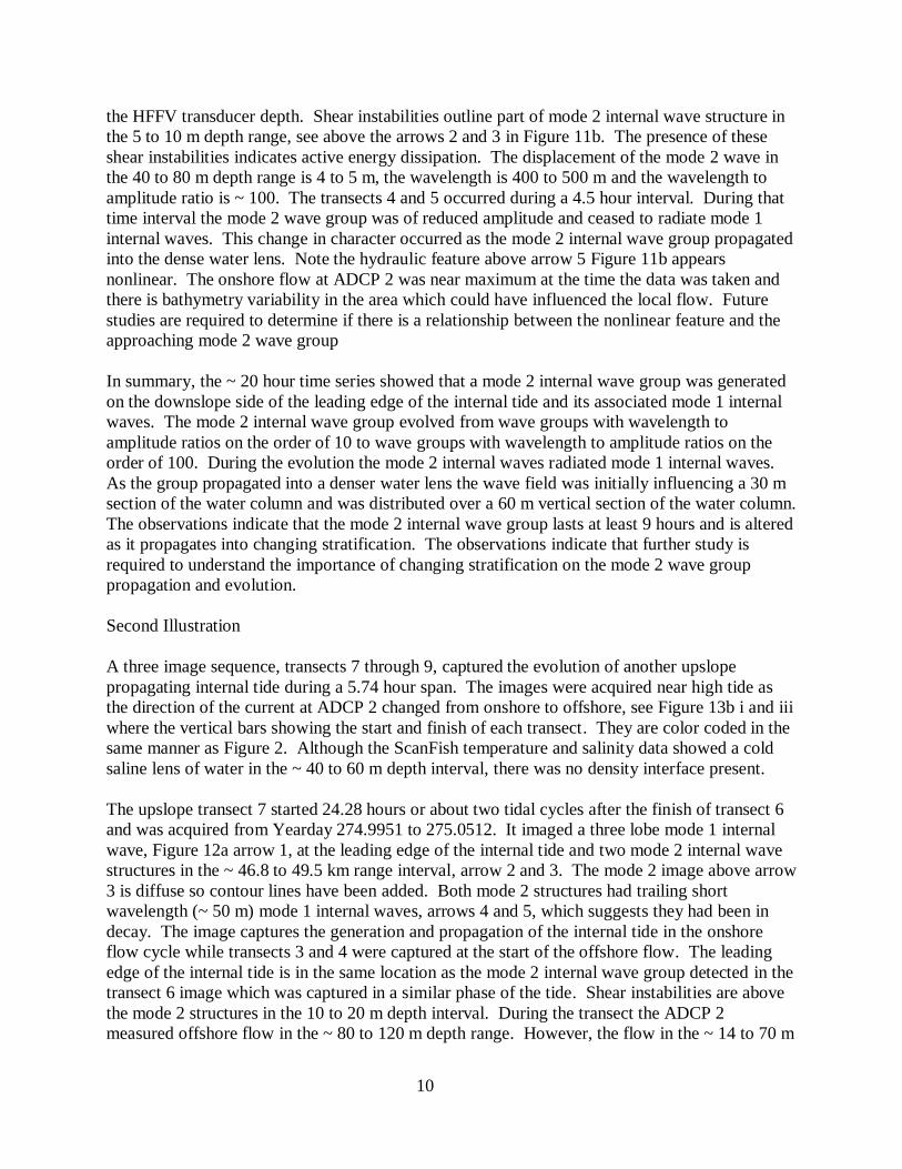
The upslope transect 7 started 24.28 hours or about two tidal cycles after the finish of transect 6

and was acquired from Yearday 274.9951 to 275.0512. It imaged a three lobe mode 1 internal

wave, Figure 12a arrow 1, at the leading edge of the internal tide and two mode 2 internal wave

structures in the ~ 46.8 to 49.5 km range interval, arrow 2 and 3. The mode 2 image above arrow

3 is diffuse so contour lines have been added. Both mode 2 structures had trailing short

wavelength (~ 50 m) mode 1 internal waves, arrows 4 and 5, which suggests they had been in

decay. The image captures the generation and propagation of the internal tide in the onshore

flow cycle while transects 3 and 4 were captured at the start of the offshore flow. The leading

edge of the internal tide is in the same location as the mode 2 internal wave group detected in the

transect 6 image which was captured in a similar phase of the tide. Shear instabilities are above

the mode 2 structures in the 10 to 20 m depth interval. During the transect the ADCP 2

measured offshore flow in the ~ 80 to 120 m depth range. However, the flow in the ~ 14 to 70 m

11

depth range was onshore, see Figure 13b in the transect 7 time interval. The magnitude of the

shear was larger than that present in the First Illustration data set, compare Figure 2 to 13b i.

Also note that shear instabilities were more prevalent in these images than in the First Illustration

data. This image, which is distinctly different than the Figure 7 image and the ADCP data,

suggests that vertical shear impacts the mode 2 internal wave propagation, generation and decay.

A reciprocal downslope transect 8 was run from Yearday 275.0677 to 275.1201 and intercepted

the internal tide at ~ 42.4 km, arrow 1. Its upslope propagation speed referenced to the bottom

was 0.43 m/s. The mode 1 internal wave group at the leading edge of the internal tide had

evolved into a bore-like structure. In the 45 and 47 km range interval short wavelength (~ 100

m) mode 2 internal waves were generated, see arrow 2 and 3, within the longer wavelength mode

2 wave between the arrows. This wave group, was about 1.6 km further upslope from the one

noted in Figure 12a between arrow 3 and 5. The spatial separation between the leading edge of

the internal tide and the mode 2 wave group increased due to the difference in their propagation

speed. Due to the HFFV coordinate system the separation between the mode 1 and mode 2 wave

groups is larger than that shown in the image as the mode 1 wave propagated about 0.5 km

upslope as the ship moved downslope to intercept the upslope propagating mode 2 internal wave

group. A blow up of the mode 2 internal wave above arrow 2 in Figure 12b, see Figure 13a,

shows its wavelength to be ~ 100 m with a peak to peak amplitude of ~ 23 m. The wavelength to

amplitude ratio was ~ 4. The mode 2 wave was starting to shed short wavelength mode 1

waves, see arrow 3. Several shear instabilities (10 to 15 m amplitude) in the 10 to 25 m depth

interval were in the vicinity of the mode 2 wave peak and downslope from it, see between the

arrows 1 and 2. The instabilities seem to be related to the presence of mode 2 internal waves and

were observed in many of the mode 2 HFFV images. Additional enlargement of the figure is

required to clearly show the instabilities. The ADCP 2 data, see Figure 13b above the transect 8

time interval, shows that vertical current shear was still present. As an aside, the 10 to 15 m

wavelength structure of 1 to 2 m amplitude above arrow 2 was caused by surface wave induced

motion of the research vessel and should be ignored.

Upslope transect 9 occurred between Yearday 275.1917 to 275.2344 and was initiated 2.15 hours

after the completion of transect 8. A 3 km long mode 2 internal wave group was imaged. The

leading edge was about 200 m downslope from ADCP 2, see Figure 14a arrow 1 to arrow 2. The

internal tide had propagated upslope to the left of range point 45 km and the mode 1 internal

waves associated with it are above and to the left of arrow 3. The mode 2 group was composed

of several shortwave length (100 to 200 m) mode 2 internal waves. The current was offshore but

still with vertical shear, see Figure 13b. An enlargement, Figure 14b, shows the character of the

embedded short period mode 2 internal waves, some are marked with the arrows 1-4. The

individual mode 2 waves are not shedding short wavelength mode 1 internal waves. The leading

mode 2 internal wave, arrow 1, could be related to the mode 2 internal wave above arrow 2 in

Figure 12 as the mode 2 wave propagation speed adjusted for downslope current would place it

close to the observed position.

In summary, the transects 7 through 9 show the evolution of an internal tide and its associated

mode 2 internal waves in the immediate vicinity of the ADCP 2 for a ~ 5.7 hour period. The

images indicate the mode 2 waves are sometimes associated with shear instabilities, have a range

of pycnocline vertical displacement amplitudes and are present when there is vertical shear in the

12

water column. The images suggest that the mode 2 wave groups may be undergoing continuous

decay and regeneration as they propagate upslope. One must remember that the interpretation of

the images is compounded by the along-shelf transport which was ~ 0.2 m/s. This current can

transport water and propagating mode 2 internal waves from ~2 km upstream into the R/V

transect 9 path in the same time interval as the repeated observations.

Third Illustration

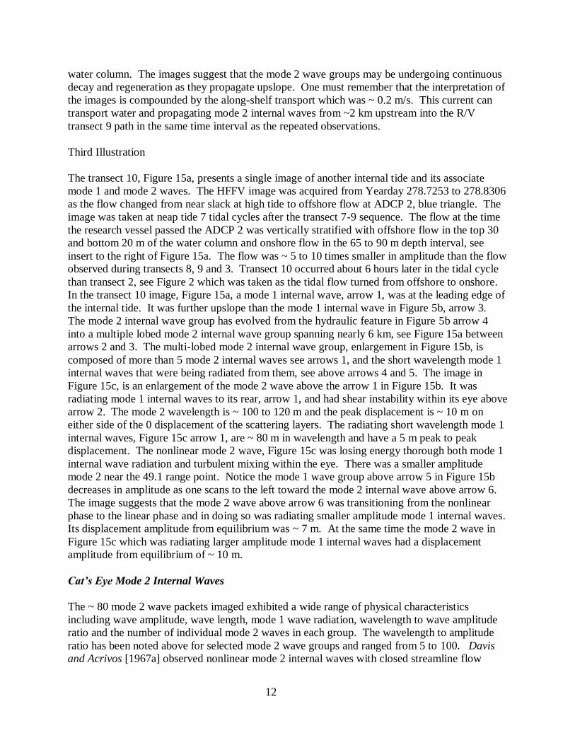
The transect 10, Figure 15a, presents a single image of another internal tide and its associate

mode 1 and mode 2 waves. The HFFV image was acquired from Yearday 278.7253 to 278.8306

as the flow changed from near slack at high tide to offshore flow at ADCP 2, blue triangle. The

image was taken at neap tide 7 tidal cycles after the transect 7-9 sequence. The flow at the time

the research vessel passed the ADCP 2 was vertically stratified with offshore flow in the top 30

and bottom 20 m of the water column and onshore flow in the 65 to 90 m depth interval, see

insert to the right of Figure 15a. The flow was ~ 5 to 10 times smaller in amplitude than the flow

observed during transects 8, 9 and 3. Transect 10 occurred about 6 hours later in the tidal cycle

than transect 2, see Figure 2 which was taken as the tidal flow turned from offshore to onshore.

In the transect 10 image, Figure 15a, a mode 1 internal wave, arrow 1, was at the leading edge of

the internal tide. It was further upslope than the mode 1 internal wave in Figure 5b, arrow 3.

The mode 2 internal wave group has evolved from the hydraulic feature in Figure 5b arrow 4

into a multiple lobed mode 2 internal wave group spanning nearly 6 km, see Figure 15a between

arrows 2 and 3. The multi-lobed mode 2 internal wave group, enlargement in Figure 15b, is

composed of more than 5 mode 2 internal waves see arrows 1, and the short wavelength mode 1

internal waves that were being radiated from them, see above arrows 4 and 5. The image in

Figure 15c, is an enlargement of the mode 2 wave above the arrow 1 in Figure 15b. It was

radiating mode 1 internal waves to its rear, arrow 1, and had shear instability within its eye above

arrow 2. The mode 2 wavelength is ~ 100 to 120 m and the peak displacement is ~ 10 m on

either side of the 0 displacement of the scattering layers. The radiating short wavelength mode 1

internal waves, Figure 15c arrow 1, are ~ 80 m in wavelength and have a 5 m peak to peak

displacement. The nonlinear mode 2 wave, Figure 15c was losing energy thorough both mode 1

internal wave radiation and turbulent mixing within the eye. There was a smaller amplitude

mode 2 near the 49.1 range point. Notice the mode 1 wave group above arrow 5 in Figure 15b

decreases in amplitude as one scans to the left toward the mode 2 internal wave above arrow 6.

The image suggests that the mode 2 wave above arrow 6 was transitioning from the nonlinear

phase to the linear phase and in doing so was radiating smaller amplitude mode 1 internal waves.

Its displacement amplitude from equilibrium was ~ 7 m. At the same time the mode 2 wave in

Figure 15c which was radiating larger amplitude mode 1 internal waves had a displacement

amplitude from equilibrium of ~ 10 m.

Cat’s Eye Mode 2 Internal Waves

The ~ 80 mode 2 wave packets imaged exhibited a wide range of physical characteristics

including wave amplitude, wave length, mode 1 wave radiation, wavelength to wave amplitude

ratio and the number of individual mode 2 waves in each group. The wavelength to amplitude

ratio has been noted above for selected mode 2 wave groups and ranged from 5 to 100. Davis

and Acrivos [1967a] observed nonlinear mode 2 internal waves with closed streamline flow

13

during their tank experiments, see their Figure 5. The image of one mode 2 internal wave in a ~ 7

km long mode 2 internal wave train had similar structure to the Davis and Acrivos [1967a]

observation, see Figure 16a. The wave peak to peak amplitude was ~ 30 m and wavelength was

~ 155 m for a wavelength to amplitude ratio of ~ 5. A cat’s eye structure suggesting closed

streamlines is clearly visible above arrow 1, as is the initiation of the shedding of energy via

mode 1 internal waves and small scale shear instabilities above and to the right of arrow 2.

Along Shelf Transect Observation

A mode 2 internal wave group was imaged twice as the R/V entered and completed an along-

shelf transect, see Figure 16b and c. The detections were at both ends of the along-shelf transect

and in the vicinity of the white circles that bound the along-shelf transect line in Figure 1. The

extent of the imaged mode 2 wave packet is shown by the red line on the insert in the upper right

corner of Figure 1. The detections were separated by 1.2 hour and 11.92 km. They are part of

the same mode 2 internal wave packet which was aligned along the shelf as the HFFV image

acquired along the transect line remained in a thickened scattering layer to the rear of leading

edge of the mode 2 wave packet for most of the transect. This observation indicates the mode 2

internal waves extend continuously at least 11.92 km along the shelf. The peak to peak

wavelength was 90 to 100 m and the peak to peak amplitude was ~ 22 m resulting in a

wavelength to amplitude ratio of about 4. Mode 1 internal waves appeared to be radiating from

individual mode 2 waves within the group, see arrow 3, Figure 16b and arrow 4 Figure 16c. The

mode 2 internal wave groups did not have identical shape. Although similar in shape the data

indicates there could be a loss of mode 2 internal wave spatial coherence along the shelf. The

amount of lateral correlation length variability will determine the accuracy of energy dissipation

rates estimated from multiple intercepts of mode 2 internal wave groups.

Mode 2 Internal Wave Generated By Flow Over Local Bathymetry

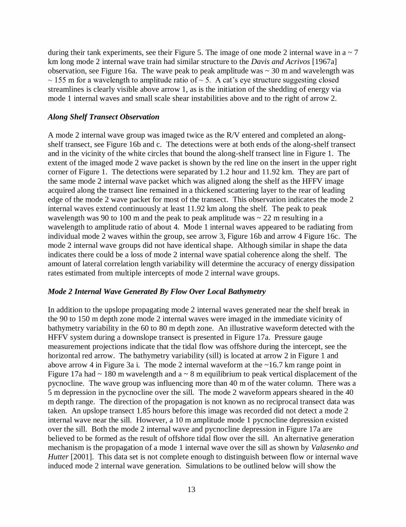
In addition to the upslope propagating mode 2 internal waves generated near the shelf break in

the 90 to 150 m depth zone mode 2 internal waves were imaged in the immediate vicinity of

bathymetry variability in the 60 to 80 m depth zone. An illustrative waveform detected with the

HFFV system during a downslope transect is presented in Figure 17a. Pressure gauge

measurement projections indicate that the tidal flow was offshore during the intercept, see the

horizontal red arrow. The bathymetry variability (sill) is located at arrow 2 in Figure 1 and

above arrow 4 in Figure 3a i. The mode 2 internal waveform at the ~16.7 km range point in

Figure 17a had ~ 180 m wavelength and a ~ 8 m equilibrium to peak vertical displacement of the

pycnocline. The wave group was influencing more than 40 m of the water column. There was a

5 m depression in the pycnocline over the sill. The mode 2 waveform appears sheared in the 40

m depth range. The direction of the propagation is not known as no reciprocal transect data was

taken. An upslope transect 1.85 hours before this image was recorded did not detect a mode 2

internal wave near the sill. However, a 10 m amplitude mode 1 pycnocline depression existed

over the sill. Both the mode 2 internal wave and pycnocline depression in Figure 17a are

believed to be formed as the result of offshore tidal flow over the sill. An alternative generation

mechanism is the propagation of a mode 1 internal wave over the sill as shown by Valasenko and

Hutter [2001]. This data set is not complete enough to distinguish between flow or internal wave

induced mode 2 internal wave generation. Simulations to be outlined below will show the

14

complexity of the flow over the sill generation mechanism and the potential difficulties of

differentiating between the generation mechanisms.

A second observation of a mode 2 internal wave group located in the vicinity of bathymetry

variability occurred when the research vessel was moored in 70 m of water at the eastern edge of

a slope in the bathymetry, see the red triangle near the red asterisk above arrow 1 in Figure 1 and

arrow 3 in Figure 3a. A mode 2 internal wave group, see Figure 17b, was imaged as it

propagated by the research vessel. The HFFV data shows the temporal response of the mid-

depth pycnocline to the passing mode 2 internal wave, arrow 1. The period was ~ 3 min (note

there are 172 sec in a .002 Yearday time step). The average flow measured at the time with the

shipboard ADCP was depth dependent onshore in the range of ~ 0.14 m/s. It is assumed the

mode 2 internal wave was propagating upslope as it was preceded by an upslope propagating

internal tide with a leading edge mode 1 internal wave group. The mode 2 internal wave

appeared about 5.08 hours after the leading edge of the internal tide and is estimated to have

been between 3.66 and 6 km downslope at the time of the internal tide intercept. The mode 2

internal wave groups described in the previous sections were 4 to 6 km behind the leading edge

of the internal tide near the 44 km range interval, and due to the speed difference between the

mode 1 and 2 internal waves they would be expected to arrive at the moored R/V about 19 hours

after the leading edge of the internal tide. The 5 hour difference in arrival time for the mode 2

internal wave group shown in Figure 17b indicates it was generated locally. The bathymetry

variability above arrows 5 and 6 Figure 3a is at the right range interval to be the generation site

for the mode 2 internal wave group that arrived at the research vessel ~ 5 hours after the internal

tide. An in-water mode 2 wave propagation speed of 0.2 m/s was assumed.

Acoustic signals scattered from the rosette as it was being raised and lower created the v shaped

pattern in the 278.495 to 278.5025 time span, see Figure 17. The density (green), temperature

(T white) and salinity ( S blue) measured by the CTD on the rosette during a down and up cast

cycle (the diagonal lines within the curves) just before the mode 2 internal wave’s arrival are

plotted. The CTD data show turbulence induced variability in T and S in the vicinity of shear

instabilities in the 5 to 15m depth range, the large gradient in T and S at the top of the

pycnocline and T and S gradients within the pycnocline. The step structure in the

measurements near 35 m becomes clearer in the HFFV image above arrow 1. The horizontal

line at 11 m to the right of Yearday 278.505 is caused by the rosette which was being held

stationary at that depth to record the temperature and salinity fluctuations caused by the shear

instabilities in the depth range.

Simulations, to be discussed below, will replicate the above observations and will show that

mode 2 waves generated in the vicinity of local bathymetry variability by currents will propagate

either onshore or offshore depending on the direction of the tidal flow during their generation

periods.

Gravity Currents

As mentioned in the introduction, gravity currents have been suggested as a possible mechanism

for mode 2 internal wave generation. A number of the ScanFish transects have been examined

for evidence of density structure that could be the result of, or cause gravity currents near the

15

pycnocline. The range versus depth plot of temperature, salinity and density (Tow yo7 YD

272.4728 to 272.6451) Figure 3a i and ii and b i, illustrate the variability encountered in the

temperature and salinity fields along a ~28 km cross-shelf transect in the ~ 65 to 150 m water

depth range. Several distinct water masses can be identified by comparing the temperature and

salinity plots. They range from cold fresh shelf water in the 40 to 64 m depth range in the 6 to

12 km range interval to somewhat warmer salty slope water in the 70 to 140 m depth interval in

the ~33 to 51 km range interval. Also note a cold less saline water mass in the 30 to 60 m depth

range in the ~ 43 to 53 km range interval. As noted, the majority of the mode 2 internal

detections (red Xs on the 5 m depth line) were in the range interval from 40 km to 55 km. The

density variability in that range interval, see Figure 3b i and 8a and b was relatively uniform.

The range resolution of the ScanFish measurements was decreasing in this range interval due to

the increased ScanFish cycle time caused by increasing water depth. The density in the 10 to 40

m depth interval in the ~ 43 to 55 km range interval was greater than the shoreward density field.

However, the data did not suggest shoreward transport was occuring in the vicinity of the

pycnocline. The ADCP 2 did detect an offshore current or jet in the 40 to 50 m depth range at

the ~ 45 km mooring point. The offshore flowing jet was persistent during some onshore flow

periods, but not all. Although there does not seem to be a correlation between the presence of

the jet and mode 2 internal wave formation there is not enough range dependent ADCP data

(multiple closely spaced cross shelf ADCP moorings) in the mode 2 internal wave detection zone

to completely understand the jet’s spatial temporal distribution and its interaction with the

upslope propagating internal tide and mode 2 internal wave groups. They both reside in the

same section of the water column and appear to be present at the same time. Further experiment

is required to resolve the issue.

Shipboard Radar Observations

Mode 1 internal wave generated surface roughness that caused radar backscatter was noted only

a few times during the experiment. This occurred when the pycnocline at the base of the ~ 30 m

mixed layer was displaced (as simultaneously observed by the acoustic backscattering system)

close to the ocean surface (10 to 15 m) by the internal tide or associated mode 1 internal waves.

No radar observations were associated with mode 2 internal waves. Due to the depth of the

mixed layer, radar observations did not provide any information concerning the presence of

mode 2 internal waves and only occasionally detected the presence of mode 1 internal waves

during the experiment period.

Summary of Observations

Key observations from the above data set are:

1. Upslope propagating mode 2 internal waves are generated in the vicinity of the shelf

break in a ~ 15 range interval where the water depth ranged from ~ 90 to 150 m, see

Figure 1. The mode 2 internal wave formation occurs in association with the

formation of an upslope propagating internal tide and its dispersive leading edge short

wavelength mode 1 internal waves. The mode 2 internal wave groups are downslope

or to the rear of the leading edge of the internal tide. The initiation of the shoreward

propagating internal tide is correlated with slacking offshore flow and the

16

development of onshore flow. A hydraulic feature generated with the offshore flow is

involved in the upslope propagating internal tide generation. The internal tide and

associated leading edge mode 1 internal waves propagation speed ranged from ~0.5

to 0.8 m/s. Over time, the mode 1 internal waves separated from the mode 2 internal

wave groups whose propagation speed was ~ 0.2 m/s. As a result, the mode 2

internal wave packets were displaced to the rear of the leading edge of the internal

and over time due to the increasing spatial separation can appear to be unrelated to

the internal tide.

2. The mode 2 internal waves were linear or weakly nonlinear (long wavelength

compared to amplitude) and nonlinear (short wavelength compared to amplitude) in

character. The spatial extent of the mode 2 packet groups was ~ 1 to 7 km, and their

peak to peak amplitudes ranged from a few meters to > 30 meters. The wavelength of

individual mode 2 waves ranged from ~ 50 m to 1 km or more. On occasion the

mode 2 internal waves were observed with closed streamline (cat’s eyes) like

structure. The mode 2 wavelength to amplitude ratios ranged from 4 to 200.

3. Nonlinear mode 2 internal wave packets were observed to radiate mode 1 internal

waves, as also observed by Shroyer et al. [2010], and exhibited turbulent mixing via

shear instability as they propagated shoreward into 80 to 90 m water. In one case, as

they propagated shoreward and encountered a lens of dense water they evolved into

longer wavelength smaller amplitude mode 2 waves which did not radiate mode 1

internal waves. The impact of the dense water lens on the mode 2 internal wave

group evolution needs to be quantified.

4. Mode 2 internal wave groups were observed to extend more than 11 km along-shelf

near the shelf break. The observation suggests that the mode 2 internal waves will be

found continuously along the same sections of the shelf where internal tides and

associated mode 1 internal waves are generated.

5. Separate from the observations in the proximity of the shelf break mode 2 waves were

also detected on the shelf near bathymetry variability in ~ 70 m or less of water. The

propagation direction of these waves was not determined uniquely as multiple

observations on each observed wave group were not made. In one case, shoreward

propagation was inferred. Numerical simulations, to be presented in the next section,

show that mode 2 internal waves generated by tidal flow or mode 1 internal wave

propagation over sill-like structures can propagate either onshore or offshore

depending on the direction of the local current flow or mode 1 propagation direction

over the sill.

6. The multiple HFFV images of nonlinear mode 2 internal waves radiating short wave

length mode 1 internal wave groups indicates that the mode 2 internal waves are a

source for continental shelf short wavelength mode 1 internal wave population. The

magnitude of the contribution needs to be quantified.

17

4. Simulation

The Shen Non-hydrostatic Model for Coastal Oceans (SNMCO) Shen and Evans [2004] was

used to simulate tidal flow over variable bathymetry using a density field that replicated some

aspects of the cross-shelf transect density field described above.

SNCOM is a free surface three dimensional fully-nonhydrostatic coastal flow model which uses

terrain-following grids, has slope-limited advection terms and accommodates density

stratification. The model features standard and open boundaries, finite-difference operations on

a curvilinear grid, a multi-grid flow solver, and accurate vertical integrals when using the default

vertical cosine grid. The two dimensional simulations that are presented below were done using

variable horizontal grid spacing ranging from 10 to over 250 m and a 97 point vertical cosine

grid. The depth of the water typically ranged from 60 m to 250 m. The finest vertical grid

spacing occurred at the surface and bottom with spacing dz=0.016 and 0.067 m for 60 and 250

m water depths, respectively. At mid water depth, the vertical resolution was the coarsest with

spacing 0.98 m in 60 m water and 4.09 m in 250 m of water. The variable vertical grid spacing

is a feature of the model’s cosine grid, and cannot be changed without losing the highly accurate

vertical integrals which are very important to this code. In the simulations a tide was created by

generating a 0.48 m displacement with a period of 12.4 hours at the right wall of the simulation

space.

The results of four simulations which used increasing water mass and bathymetry complexity are

discussed. Three simulated tidal flow over bathymetric variability including sill like structures.

The fourth simulated the upslope propagation of an internal tide generated offshore of the shelf

break. The simulation results are presented by plotting isopycnal lines to allow inter-comparison

with the HFFV images. The characteristics of each of the simulations follow.

1. The first simulation used a 100 km tow dimensional section with 50 m water

depth from 0 to 48 km, a 50 m sill and a 100 km section of 100 m water, see

Figure 18a. The simulation was initialized with a range independent two layer

fluid separated by a pycnocline.

2. The second simulation used a 200 km section along the research vessel cross-shelf

transect tract with a bottom depth ranging from 60 m to 250 m. The continental

shelf break occurred at a depth of ~ 150 m near 55 km. The bottom bathymetry

replicated a low pass filtered version of the NOAA bathymetry data, Figure 1a,

taken along a 35 km section of the research vessel track from shelf break

shoreward. Small scale (< ~5 km) bathymetry variability on the shelf was

removed. The range dependent temperature and salinity profile was replicated,

within the SNMCO code grid resolution, the larger scales of the temperature and

salinity field measured during the ScanFish tow 7, see Figure 3a.

3. The third simulation was the same as item 2 except small scale bathymetry

variability shoreward of the continental shelf break was included.

18

4. The fourth simulation modeled the upslope propagation of an internal tide

generated at a distance to the east of the shelf break. The simulation was done to

determine if mode 2 internal waves could be generated by an offshore generated

upslope propagating internal tide. The bottom bathymetry and the range

dependent temperature and salinity fields were the same as that used in the third

simulation.

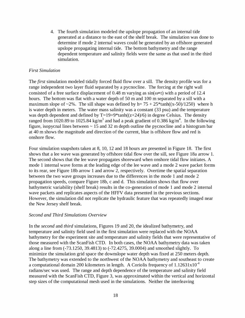
First Simulation

The first simulation modeled tidally forced fluid flow over a sill. The density profile was for a

range independent two layer fluid separated by a pycnocline. The forcing at the right wall

consisted of a free surface displacement of 0.48 m varying as sin(t) with a period of 12.4

hours. The bottom was flat with a water depth of 50 m and 100 m separated by a sill with a

maximum slope of ~2%. The sill shape was defined by h= 75 + 25*tanh((x-50)/1250) where h

is water depth in meters. The water mass salinity was a constant (33 psu) and the temperature

was depth dependent and defined by T=19+9*tanh((z+24)/6) in degree Celsius. The density

ranged from 1020.89 to 1025.84 kg/m3 and had a peak gradient of 0.386 kg/m

4. In the following

figure, isopycnal lines between ~ 15 and 32 m depth outline the pycnocline and a histogram bar

at 40 m shows the magnitude and direction of the current, blue is offshore flow and red is

onshore flow.

Four simulation snapshots taken at 8, 10, 12 and 18 hours are presented in Figure 18. The first

shows that a lee wave was generated by offshore tidal flow over the sill, see Figure 18a arrow 1.

The second shows that the lee wave propagates shoreward when onshore tidal flow initiates. A

mode 1 internal wave forms at the leading edge of the lee wave and a mode 2 wave packet forms

to its rear, see Figure 18b arrow 1 and arrow 2, respectively. Overtime the spatial separation

between the two wave groups increases due to the differences in the mode 1 and mode 2

propagation speeds, compare Figure 18b, c and d. This simulation shows that flow over

bathymetric variability (shelf break) results in the co-generation of mode 1 and mode 2 internal

wave packets and replicates aspects of the HFFV data presented in the previous sections.

However, the simulation did not replicate the hydraulic feature that was repeatedly imaged near

the New Jersey shelf break.

Second and Third Simulations Overview

In the second and third simulations, Figures 19 and 20, the idealized bathymetry, and

temperature and salinity field used in the first simulation were replaced with the NOAA

bathymetry for the experiment site and temperature and salinity fields that were representative of

those measured with the ScanFish CTD. In both cases, the NOAA bathymetry data was taken

along a line from (-73.1250, 39.4813) to (-72.4275, 39.0004) and smoothed slightly. To

minimize the simulation grid space the downslope water depth was fixed at 250 meters depth.

The bathymetry was extended to the northwest of the NOAA bathymetry and southeast to create

a computational domain 200 kilometers in length. A Coriolis frequency of 1.12631x10-4

radians/sec was used. The range and depth dependence of the temperature and salinity field

measured with the ScanFish CTD, Figure 3, was approximated within the vertical and horizontal

step sizes of the computational mesh used in the simulations. Neither the interleaving

19

temperature and salinity lenses measured by the CTD or the current jets measured with the

ADCP 2 were replicated in the simulation’s initialization. The current speed histogram bars at

40 m and 80 m indicate the relative magnitude and direction of the current, blue is offshore flow

and red is onshore flow.

The initial conditions used were:

Temperature(x, z) = 16 + 5*tanh((z-zc)/104)+ tanh((x-xc)/10

3)

Salinity(x, z) = 33.5 + 0.5* tanh((x-xc)/10 3)

where zc = 42.5 + 7.5*tanh((x-8.7x104)/10

4) and xc = 5.95x10

4 - 2500 *tanh((z+35)/6)

Velocity (v(x; z)) was chosen such that f*dv/dz=-g/ddx, which balances out the horizontal

variability of the density in the initial conditions u = 0 and w = 0.

The forcing was 𝜕𝐹

𝜕𝑥= 𝑢𝐹 ∗ 𝑓𝑀2 ∗ sin(𝑓𝑀2 ∗ 𝑡)

over the computational domain. The values for 𝑢𝐹 used during the simulations ranged from

0.025 m/s to 0.05 m/s. The peak flows tend to be 10-20 times this value. The frequency of the

M2 tide ( fM2) was12.4 hr.

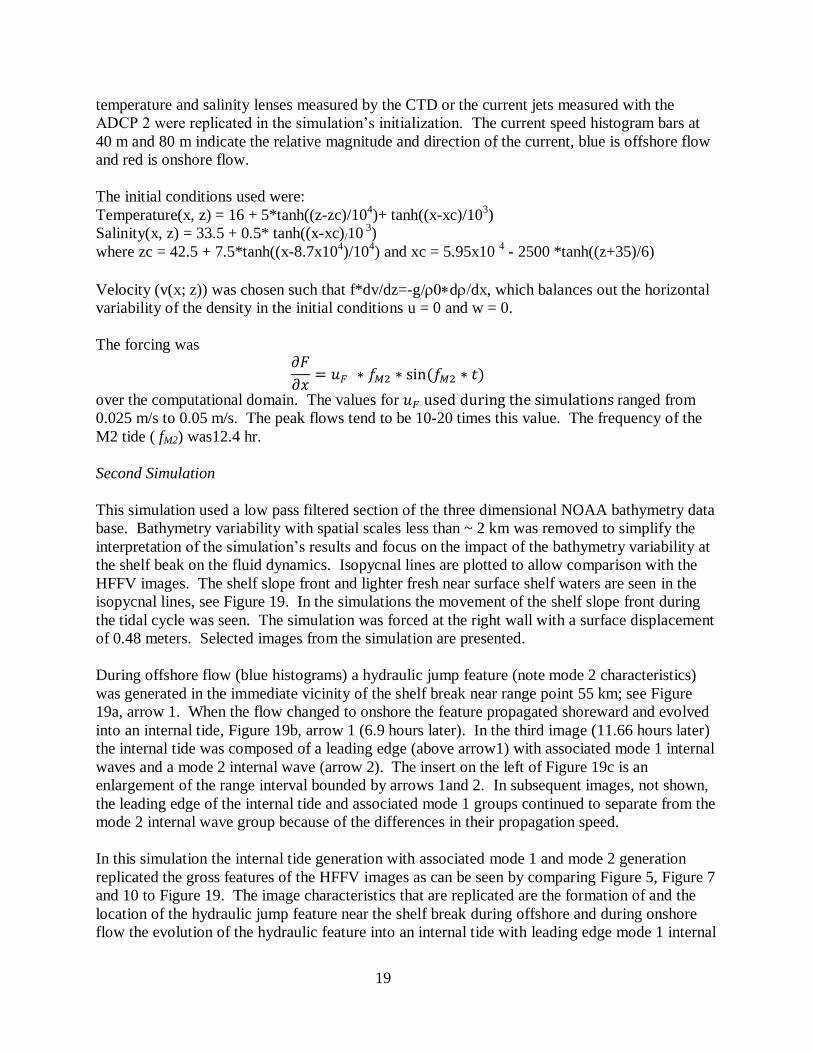
Second Simulation

This simulation used a low pass filtered section of the three dimensional NOAA bathymetry data

base. Bathymetry variability with spatial scales less than ~ 2 km was removed to simplify the

interpretation of the simulation’s results and focus on the impact of the bathymetry variability at

the shelf beak on the fluid dynamics. Isopycnal lines are plotted to allow comparison with the

HFFV images. The shelf slope front and lighter fresh near surface shelf waters are seen in the

isopycnal lines, see Figure 19. In the simulations the movement of the shelf slope front during

the tidal cycle was seen. The simulation was forced at the right wall with a surface displacement

of 0.48 meters. Selected images from the simulation are presented.

During offshore flow (blue histograms) a hydraulic jump feature (note mode 2 characteristics)

was generated in the immediate vicinity of the shelf break near range point 55 km; see Figure

19a, arrow 1. When the flow changed to onshore the feature propagated shoreward and evolved

into an internal tide, Figure 19b, arrow 1 (6.9 hours later). In the third image (11.66 hours later)

the internal tide was composed of a leading edge (above arrow1) with associated mode 1 internal

waves and a mode 2 internal wave (arrow 2). The insert on the left of Figure 19c is an

enlargement of the range interval bounded by arrows 1and 2. In subsequent images, not shown,

the leading edge of the internal tide and associated mode 1 groups continued to separate from the

mode 2 internal wave group because of the differences in their propagation speed.

In this simulation the internal tide generation with associated mode 1 and mode 2 generation

replicated the gross features of the HFFV images as can be seen by comparing Figure 5, Figure 7

and 10 to Figure 19. The image characteristics that are replicated are the formation of and the

location of the hydraulic jump feature near the shelf break during offshore and during onshore

flow the evolution of the hydraulic feature into an internal tide with leading edge mode 1 internal

20

waves and following mode 2 waves. The spatial location of the simulated mode 2 internal wave

group replicated the HFFV images. Due to grid step size limitations the simulation does not

replicate the observed mode 2 to short wavelength mode 1 internal wave conversion process.

The simulation did not replicate the complexity of the internal wave fields seen in the HFFV

images especially in the range interval shoreward of the 35 km range point. The simulation did

replicate the hydraulic feature seen in the HFFV images near the shelf break during both on and

offshore flow conditions, see arrow 3 Figure 19c.

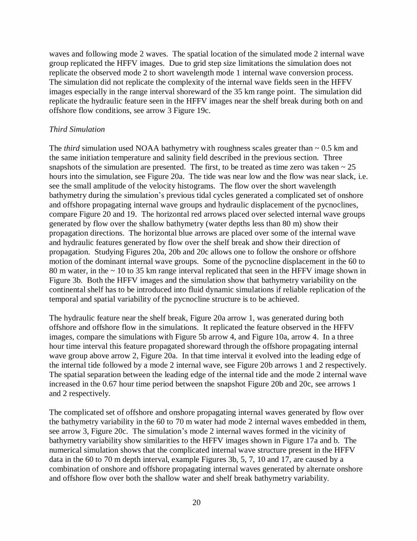
Third Simulation

The third simulation used NOAA bathymetry with roughness scales greater than ~ 0.5 km and

the same initiation temperature and salinity field described in the previous section. Three

snapshots of the simulation are presented. The first, to be treated as time zero was taken ~ 25

hours into the simulation, see Figure 20a. The tide was near low and the flow was near slack, i.e.

see the small amplitude of the velocity histograms. The flow over the short wavelength

bathymetry during the simulation’s previous tidal cycles generated a complicated set of onshore

and offshore propagating internal wave groups and hydraulic displacement of the pycnoclines,

compare Figure 20 and 19. The horizontal red arrows placed over selected internal wave groups

generated by flow over the shallow bathymetry (water depths less than 80 m) show their

propagation directions. The horizontal blue arrows are placed over some of the internal wave

and hydraulic features generated by flow over the shelf break and show their direction of

propagation. Studying Figures 20a, 20b and 20c allows one to follow the onshore or offshore

motion of the dominant internal wave groups. Some of the pycnocline displacement in the 60 to

80 m water, in the ~ 10 to 35 km range interval replicated that seen in the HFFV image shown in

Figure 3b. Both the HFFV images and the simulation show that bathymetry variability on the

continental shelf has to be introduced into fluid dynamic simulations if reliable replication of the

temporal and spatial variability of the pycnocline structure is to be achieved.

The hydraulic feature near the shelf break, Figure 20a arrow 1, was generated during both

offshore and offshore flow in the simulations. It replicated the feature observed in the HFFV

images, compare the simulations with Figure 5b arrow 4, and Figure 10a, arrow 4. In a three

hour time interval this feature propagated shoreward through the offshore propagating internal

wave group above arrow 2, Figure 20a. In that time interval it evolved into the leading edge of

the internal tide followed by a mode 2 internal wave, see Figure 20b arrows 1 and 2 respectively.

The spatial separation between the leading edge of the internal tide and the mode 2 internal wave

increased in the 0.67 hour time period between the snapshot Figure 20b and 20c, see arrows 1

and 2 respectively.

The complicated set of offshore and onshore propagating internal waves generated by flow over

the bathymetry variability in the 60 to 70 m water had mode 2 internal waves embedded in them,

see arrow 3, Figure 20c. The simulation’s mode 2 internal waves formed in the vicinity of

bathymetry variability show similarities to the HFFV images shown in Figure 17a and b. The

numerical simulation shows that the complicated internal wave structure present in the HFFV

data in the 60 to 70 m depth interval, example Figures 3b, 5, 7, 10 and 17, are caused by a

combination of onshore and offshore propagating internal waves generated by alternate onshore

and offshore flow over both the shallow water and shelf break bathymetry variability.

21

Unpublished HFFV data (Orr) taken during other experiments at this site have shown shoreward

propagating mode 1 internal wave groups developing in the vicinity and shoreward of the 70 to

80 m depth interval suggesting that the shallow water bathymetry variability plays an important

part in defining the characteristics of the local internal wave field. The HFFV images and the

simulations show that any realistic simulation of internal waves on the continental shelf must

include a realistic representation of the local bathymetry and density fields.

In conclusion, the simulations and HFFV images support the interpretation of the HFFV images

in regard to mode 2 internal wave generation by flow over on shelf bathymetry variability as well

as bathymetry variability at the continental shelf break.

Fourth Simulation

Nash, Kelly, Shroyer, Moum, and Duda [2012], have suggested that upslope propagating internal

tides generated at offshore locations, that are distant from the continental shelf break, can

generate shoreward propagating internal waves that are not in phase with the tide. A simulation

was run to determine if an upslope propagating internal tide (not coupled to the local tidal flow)

would generate coupled mode 1 and mode 2 wave trains similar to those observed during this

experiment. No tide forcing was used in the simulation. The internal tide was generated by

displacing the thermocline 25 m with a 30 km wide sech function. The displacement was

centered 50 km offshore of the continental slope. A shoreward propagating internal tide of

depression with short wavelength internal wave at the leading edge was generated by the

buoyancy rebound from the displacement. The simulations have shown that the upslope

propagating internal tides generated hydraulic features (5 to 10 km wavelength) as they crossed

the shelf break as well as offshore propagating mode 2 internal wave features. However to date,

no upslope propagating coupled mode 1 and mode 2 internal waves have been generated by the

internal tide encounter with the shelf break. The simulations suggest that the upslope

propagating coupled mode 1 and mode 2 internal waves observed with the HFFV system require

offshore flow to generate the hydraulic feature from which the upslope propagating internal tide

with mode 1 and mode 2 internal waves are generated.

Overview of the Simulations

The simulations show that coupled upslope propagating mode 1 and mode 2 internal waves are

formed in a stratified water column and depth varying bathymetry when offshore flow over the

shelf break generates a hydraulic jump feature. The feature propagates shoreward with

slackening offshore flow and evolves into a shoreward propagating internal tide with mode 1

internal waves at the leading edge and mode 2 internal waves to the rear. The mode 1 and mode

2 internal wave groups separated in time due to their different propagation speeds. The location

of the mode 2 internal wave formation in the simulation replicates the location of the internal

tide, mode 1 and mode 2 internal waves observed in the HFFV images. The simulations also

indicate that offshore propagating mode 1 and mode 2 internal waves can be generated by

onshore flow over the shelf break. No HFFV imagery was taken seaward of the shelf break to

validate the simulation. In addition, the simulations replicated the HFFV observation of the

generation of both mode 1 and mode 2 internal waves by onshore and offshore flow over

bathymetry variability on the continental shelf. In the case of range independent bathymetry

22

with a sill and a range independent density field the simulations did not replicate the hydraulic

features observed in the HFFV images.

5. Conclusion

Mode 2 internal wave groups have been imaged in two zones on the New Jersey continental shelf

during the early fall when the mixed layer approached half water column depth. One zone

encompassed a ~ 15 km range interval (~90 to 150 m depth interval) extending upslope from the

continental shelf break. The second zone was in the vicinity of bathymetry variability in the ~ 60

to 80 m depth zone on the shelf. The observations were made during a ~ 7 day period before and

including neap tide.

In the ~ 15 km range interval the mode 2 internal waves were repeatedly observed to form from a

hydraulic feature which was generated during offshore flow over the continental shelf break.

The feature propagated upslope, when offshore flow slacked and turned to onshore flow, and

evolved into an upslope propagating internal tide with mode 1 internal waves at the leading edge

and upslope propagating mode 2 internal wave groups forming to the rear. The leading edge of

the internal tide and the following mode 2 internal wave groups separated over time due to

differences in propagation speed. The mode 2 internal wave groups had a variety of shapes and

evolved over time and space from waves with small wavelength to amplitude ratios (~ 5) to

waves with longer wavelength to amplitude ratios (~100). During their evolution the mode 2

internal waves shed short period mode 1 internal waves and were associated with shear

instabilities. Closed streamline structures were also observed within some mode 2 internal

waves. The mode 2 wave groups had an along shelf extent of 11.9 km. These observations and

the nearby observation of mode 2 internal waves by Shroyer et. al [2010] in a similar depth

regime suggest that the mode 2 wave groups may have a significant along shelf extent and might

be found wherever the internal tide and associated mode 1 internal waves are generated near the

shelf break. The water column conditions, which are required for the mode 2 internal wave

group generation, need to be established. There are a number of issues. Laboratory experiments

suggest they are formed when the mixed layer depths are at approximately half water column

depth. This data set was taken in a water column with a deep mixed layer which replicates to a

degree the laboratory conditions. However, Shroyer et. al [2010] have observed mode 2 internal

waves during summer time conditions with a shallow mixed layer which indicates a seasonal

study of mode 2 internal wave generation conditions is needed to define the water column and

flow conditions required for their formation including the tidal conditions, i.e. the influence of

the spring to neap tidal cycle and water column shear? Other issues include quantifying the

fraction of the short wave length mode 1 internal wave energy field spectrum in shelf waters is

generated by mode 2 internal waves and how much energy do they shed through the shear

instabilities that are associated with their propagation?

In the 60 to 80 m water the rate of mode 2 internal wave generation by flow over local

bathymetry variability needs to be quantified. What combination of mixed layer depth, current

and bathymetry height and slope conditions are required for the mode 2 internal wave generation

near on-shelf sills, and how do these waves dissipate? Is the generation driven by tidal flow or

currents related to mode 1 internal propagation past the sills?

23

The observations and simulations presented provide a glimpse into the mode 2 internal wave

generation processes and will help focus and guide future research efforts addressing their

kinematics and dynamics.

24

Acknowledgments

We thank the anomalous reviewers of the paper for their many comments and suggestions and

the editor for his encouragement. Dr. Colin Shen was a co-investigator who was to support the

interpretation of this data set with his non-hydrostatic numerical simulations. Unfortunately he

passed away at the initiation of the analysis. This report is dedicated to him. John Kemp and his

rigging team at the Woods Hole Oceanographic prepared the R/V Endeavor to accommodate a

high frequency acoustic transducer mounting system. The R/V Endeavor technical support team

provided invaluable help to obtain the tow-yo and yo-yo CTD data. Dr. Julia Hummon, The

University of Hawaii, kindly converted the R/V Endeavor ADCP data from ping files to ascii

files and provided comment as to the quality of the R/V Endeavor ADCP data. Dr. Peter

Mignerey provided MatLab scripts for the capturing and plotting of the high frequency acoustic

flow visualization data. Michael McCord designed the HFFV preamplifier/amplifiers and

provided engineering support for the system. Earl Carey’s ocean engineering and electronic

engineering support was invaluable. Robert Field was the principle investigator for the Shallow

Water Acoustic Technology experiment and is thanked for the opportunity he provided to

acquire the HFFV data during one leg of the experiment. This work was supported by the Office

of Naval Research.

25

Reference List

Apel, J. R., Badiey, M., Chiu, Ching-Shang, Finette, S., Headrick, R., Kemp, J., Lynch, J. F.,

Newhall, A., Orr, M. H., Pasewark, B. H., Tielbuerger, D., Turgut, A., Von Der Heydt, K. and

Wolf, S. (1997), An overview of the 1995 SWARM shallow water internal wave acoustic

scattering experiment, IEEE J. Oceanic Eng., 22, 465-500.

Benjamin, T. B (1967), Internal waves of permanent form in fluids of great depth, J. Fluid

Mech., 29, 559-592.

Bogucki, D. J., Redekopp, L. G., Barth, J. (2005), Internal solitary waves in the coastal mixing

and optics 1996 experiment: Multimodal structure and resuspension, J. Geophys. Res., 110,

C02024, doi:10.1029/2003JC002253.

Davis, R. E. and Acrivos, A. (1967a), Solitary internal waves in deep water, J. Fluid Mech., 29,

593-607.

Davis, R. E. and Acrivos, A. (1967b), The stability of oscillatory internal waves, J. Fluid Mech.,

30, 723-736.

Farmer, D. M., and J. D. Smith (1980), Tidal interaction of stratified flow

with a sill in Knight Inlet, Deep Sea Res., Part A, 27, 239-254.

Helfrich, K. R. and Melville, W. K. (1986), On long nonlinear internal waves over shelf-slope

topography, J. Fluid Mech. 167, 285-308

Goodman, L. (1990), Acoustic Scattering from Ocean Microstructure, J.Geophys. Res., 95,

11557-11573.

Hallock, Z. R. and R. L. Field (2005), Internal-Wave Energy Fluxes on the New Jersey Shelf, J.

Geophys. Res., 35, 3-12.

Henyey, F. S., Williams, K.; Becker, K. M., Lyons, J., Ballard, M., Camin, J., Gabel, P.,

Koszalka, I., Beitel, J. (2006), Internal Wave Measurements With a Towed CTD Chain on the

New Jersey Shelf, American Geophysical Union, Fall Meeting 2006, abstract #OS23C-02.

Mehta, A. P., B. R. Sutherland, and P. J. Kyba (2002), Interfacial gravity currents. II. Wave

Excitation, Physics of Fluids, 1, 3558-3569.

Orr, M. H. and Hess, F. R.(1978), Remote Acoustic Monitoring of Natural Suspensate

Distributions, Active Suspensate Resuspension, and Slope/Shelf Water Intrusions, J. Geophys.

Res., 83 C8,4062-4067.

Orr, M. H. (2004), Seasonal Variability of Internal Waves on the New Jersey Continental Shelf –

Observations, ASKI/TOS 2004 Ocean Research Conference, Abstract Book (http://www.aslo.org), pg. 118.

26

Nash, J. D., Kelly, S. M., Shroyer, E. L., Moum, J. N., Duda, F. T. (2012), The unpredictable

nature of internal tides on continental shelves, J. Phys. Oceanogr. 42, 1981-2000,

doi:10.1175/JPO-D-12-028.1.

Shen, C. Y., Evans, T. E. (2004), A free-surface hydrodynamic model for density-stratified flow

in the weakly to strongly non-hydrostatic regime, J. Comp. Phys., 200, 695-717,

doi:10.1016/j.jcp.2004.04.015.

Shroyer, E. L., Moum, J. N. and Nash , J. D. (2010), Mode 2 waves on the continental shelf:

Ephemeral components of the nonlinear internal wavefield, J. Geophys. Res., 115, C07001,

doi:10.1029/2009JC005605.

Smith, C., Bradley, D., Mignerey, P. and Goldstein, D. (2009), 24th Underwater Acoustics

Conference (UAC) of the Acoustical Society of Korea in Agency for Defense Development,

Jinhae on 17-18 September, 2009.

Stanton, T. K., Wiebe, P. H., Chu, D. and Goodman, L. (1994), Acoustic characterization and

discrimination of marine zooplankton and turbulence, J. Mar. Sci., 51, 469-479.

Stastna, M. and Peltier, W. R. (2005), On the resonant generation of large-amplitude internal

solitary and solitary-like waves, J. Fluid Mech., 543, 267-292,

doi:10.1017/S002211200500652X.

Vlasenko, V. I. and Hutter, K. (2001), Generation of second order mode solitary waves,

Nonlinear Processes Geophys., 8, 223-239.

Yang, Y. J., Fang, Ying, Chih, Chang, M, Ramp, S. R., Kao, C and Tang, T. Y. (2009),

Observations of second baraoclinic mode internal solitary waves on the continental slope of the

northern South China Sea, J. Geophys. Res., 114, C10003, doi: 10.1029/2009JC005318.

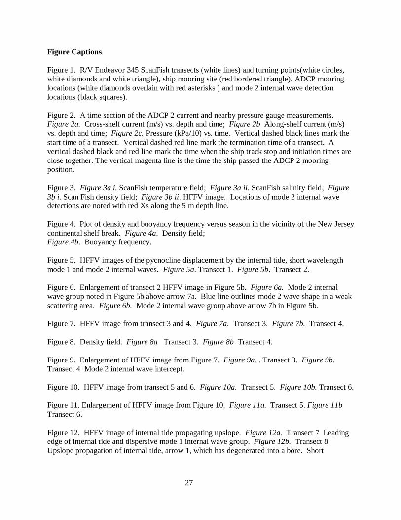
27

Figure Captions

Figure 1. R/V Endeavor 345 ScanFish transects (white lines) and turning points(white circles,

white diamonds and white triangle), ship mooring site (red bordered triangle), ADCP mooring

locations (white diamonds overlain with red asterisks ) and mode 2 internal wave detection

locations (black squares).

Figure 2. A time section of the ADCP 2 current and nearby pressure gauge measurements.

Figure 2a. Cross-shelf current (m/s) vs. depth and time; Figure 2b Along-shelf current (m/s)

vs. depth and time; Figure 2c. Pressure (kPa/10) vs. time. Vertical dashed black lines mark the

start time of a transect. Vertical dashed red line mark the termination time of a transect. A

vertical dashed black and red line mark the time when the ship track stop and initiation times are

close together. The vertical magenta line is the time the ship passed the ADCP 2 mooring

position.

Figure 3. Figure 3a i. ScanFish temperature field; Figure 3a ii. ScanFish salinity field; Figure

3b i. Scan Fish density field; Figure 3b ii. HFFV image. Locations of mode 2 internal wave

detections are noted with red Xs along the 5 m depth line.

Figure 4. Plot of density and buoyancy frequency versus season in the vicinity of the New Jersey

continental shelf break. Figure 4a. Density field;

Figure 4b. Buoyancy frequency.

Figure 5. HFFV images of the pycnocline displacement by the internal tide, short wavelength

mode 1 and mode 2 internal waves. Figure 5a. Transect 1. Figure 5b. Transect 2.

Figure 6. Enlargement of transect 2 HFFV image in Figure 5b. Figure 6a. Mode 2 internal

wave group noted in Figure 5b above arrow 7a. Blue line outlines mode 2 wave shape in a weak

scattering area. Figure 6b. Mode 2 internal wave group above arrow 7b in Figure 5b.

Figure 7. HFFV image from transect 3 and 4. Figure 7a. Transect 3. Figure 7b. Transect 4.

Figure 8. Density field. Figure 8a Transect 3. Figure 8b Transect 4.

Figure 9. Enlargement of HFFV image from Figure 7. Figure 9a. . Transect 3. Figure 9b.

Transect 4 Mode 2 internal wave intercept.

Figure 10. HFFV image from transect 5 and 6. Figure 10a. Transect 5. Figure 10b. Transect 6.

Figure 11. Enlargement of HFFV image from Figure 10. Figure 11a. Transect 5. Figure 11b

Transect 6.

Figure 12. HFFV image of internal tide propagating upslope. Figure 12a. Transect 7 Leading

edge of internal tide and dispersive mode 1 internal wave group. Figure 12b. Transect 8

Upslope propagation of internal tide, arrow 1, which has degenerated into a bore. Short

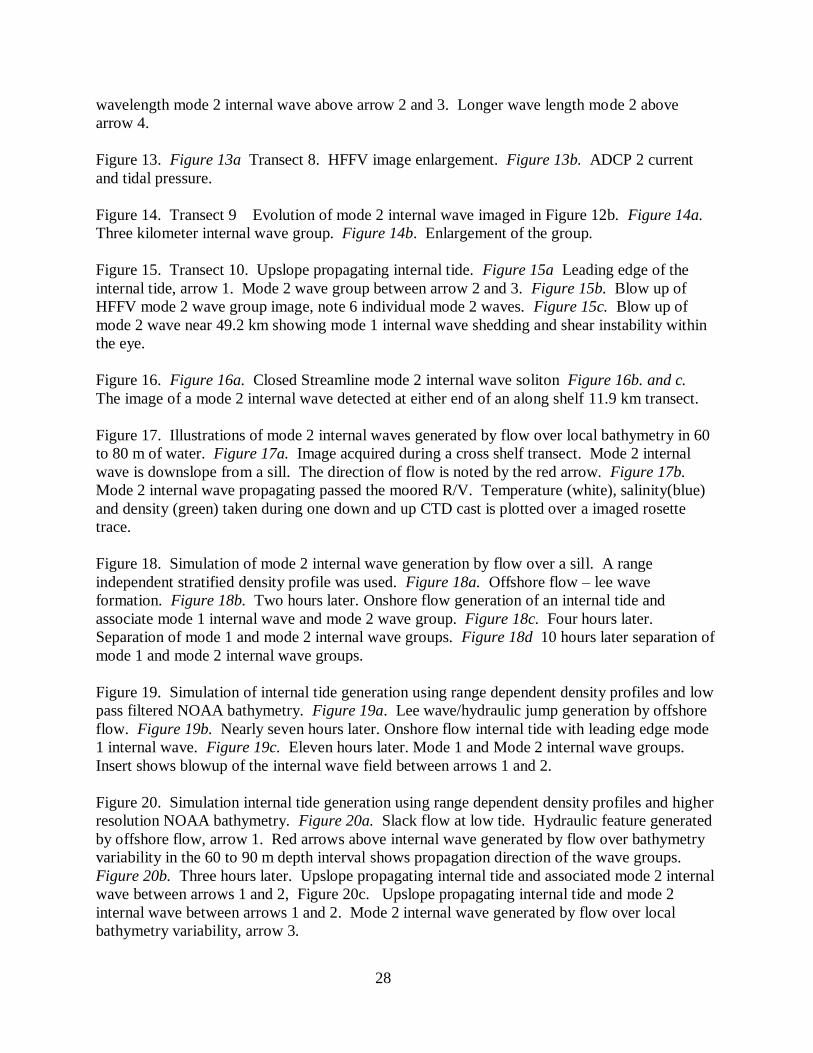
28

wavelength mode 2 internal wave above arrow 2 and 3. Longer wave length mode 2 above

arrow 4.

Figure 13. Figure 13a Transect 8. HFFV image enlargement. Figure 13b. ADCP 2 current

and tidal pressure.

Figure 14. Transect 9 Evolution of mode 2 internal wave imaged in Figure 12b. Figure 14a.

Three kilometer internal wave group. Figure 14b. Enlargement of the group.

Figure 15. Transect 10. Upslope propagating internal tide. Figure 15a Leading edge of the

internal tide, arrow 1. Mode 2 wave group between arrow 2 and 3. Figure 15b. Blow up of

HFFV mode 2 wave group image, note 6 individual mode 2 waves. Figure 15c. Blow up of

mode 2 wave near 49.2 km showing mode 1 internal wave shedding and shear instability within

the eye.

Figure 16. Figure 16a. Closed Streamline mode 2 internal wave soliton Figure 16b. and c.

The image of a mode 2 internal wave detected at either end of an along shelf 11.9 km transect.

Figure 17. Illustrations of mode 2 internal waves generated by flow over local bathymetry in 60

to 80 m of water. Figure 17a. Image acquired during a cross shelf transect. Mode 2 internal

wave is downslope from a sill. The direction of flow is noted by the red arrow. Figure 17b.

Mode 2 internal wave propagating passed the moored R/V. Temperature (white), salinity(blue)

and density (green) taken during one down and up CTD cast is plotted over a imaged rosette

trace.

Figure 18. Simulation of mode 2 internal wave generation by flow over a sill. A range

independent stratified density profile was used. Figure 18a. Offshore flow – lee wave

formation. Figure 18b. Two hours later. Onshore flow generation of an internal tide and

associate mode 1 internal wave and mode 2 wave group. Figure 18c. Four hours later.

Separation of mode 1 and mode 2 internal wave groups. Figure 18d 10 hours later separation of

mode 1 and mode 2 internal wave groups.

Figure 19. Simulation of internal tide generation using range dependent density profiles and low

pass filtered NOAA bathymetry. Figure 19a. Lee wave/hydraulic jump generation by offshore

flow. Figure 19b. Nearly seven hours later. Onshore flow internal tide with leading edge mode

1 internal wave. Figure 19c. Eleven hours later. Mode 1 and Mode 2 internal wave groups.

Insert shows blowup of the internal wave field between arrows 1 and 2.

Figure 20. Simulation internal tide generation using range dependent density profiles and higher

resolution NOAA bathymetry. Figure 20a. Slack flow at low tide. Hydraulic feature generated

by offshore flow, arrow 1. Red arrows above internal wave generated by flow over bathymetry

variability in the 60 to 90 m depth interval shows propagation direction of the wave groups.

Figure 20b. Three hours later. Upslope propagating internal tide and associated mode 2 internal

wave between arrows 1 and 2, Figure 20c. Upslope propagating internal tide and mode 2

internal wave between arrows 1 and 2. Mode 2 internal wave generated by flow over local

bathymetry variability, arrow 3.

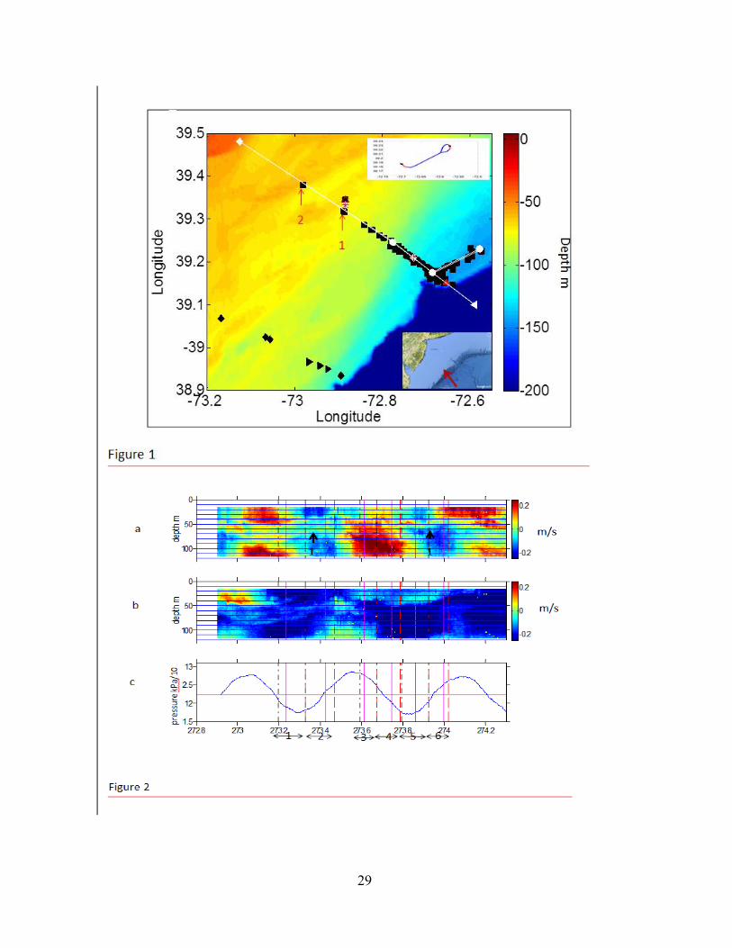
29

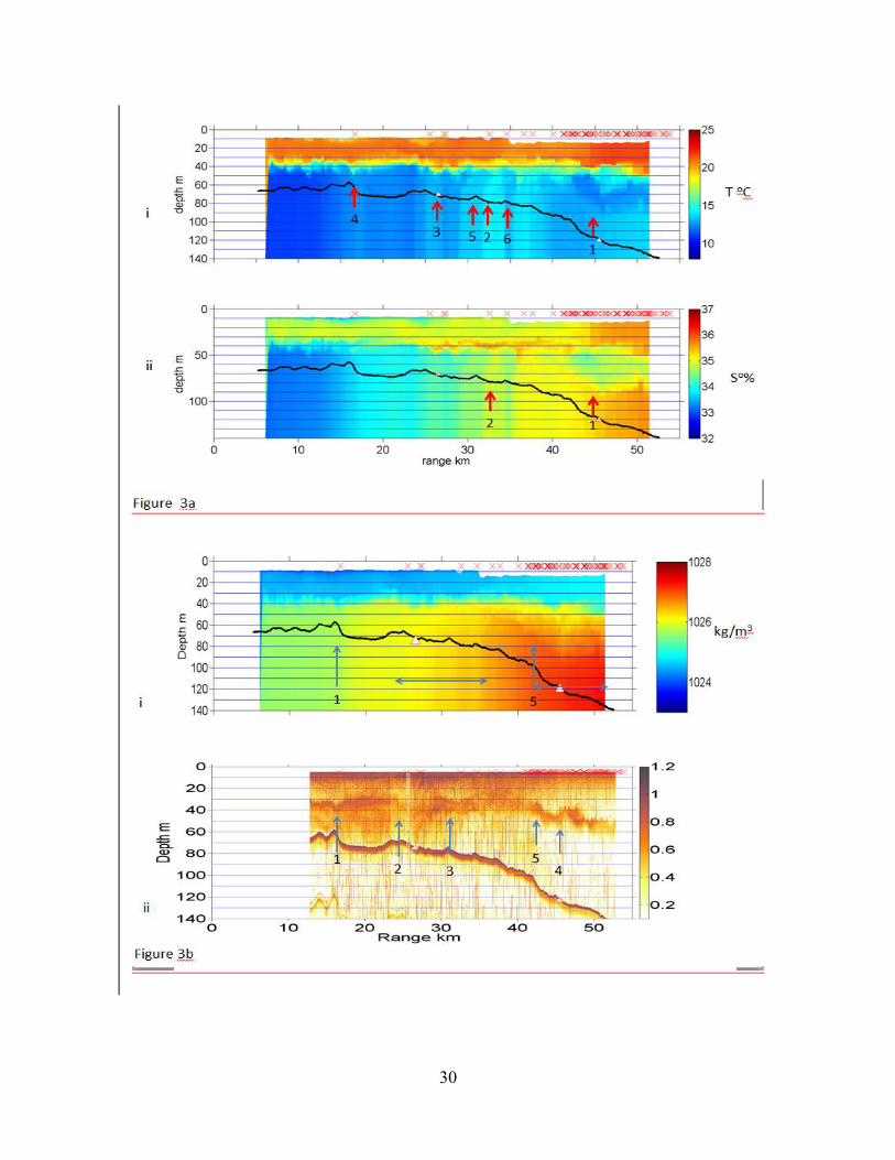
30

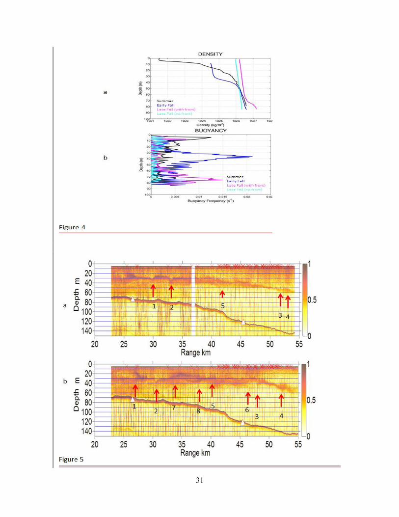
31

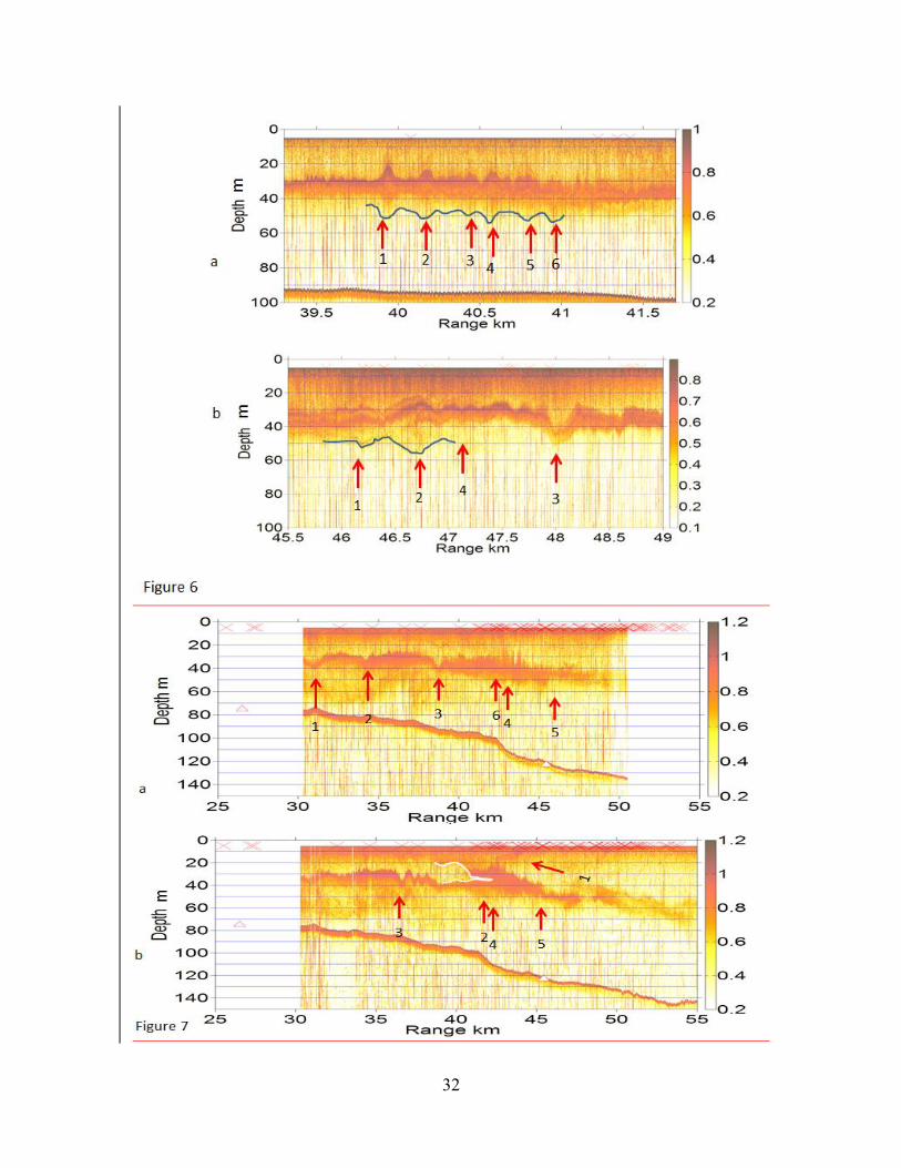
32

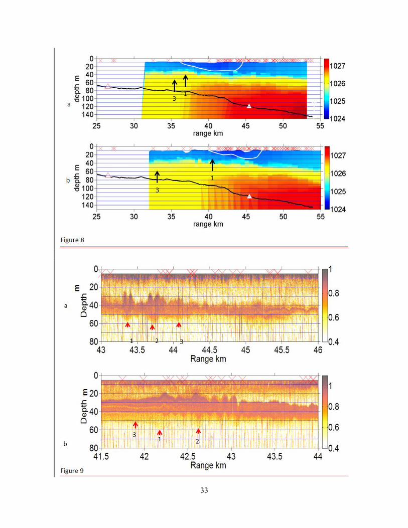
33

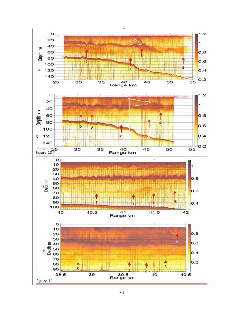
34

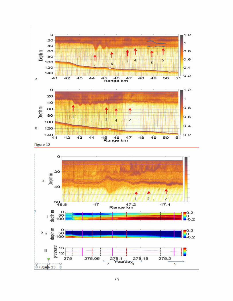
35

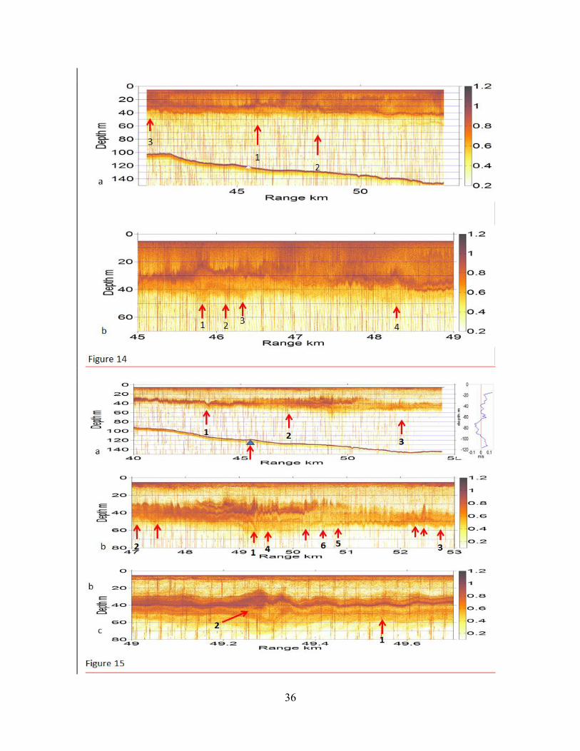
36

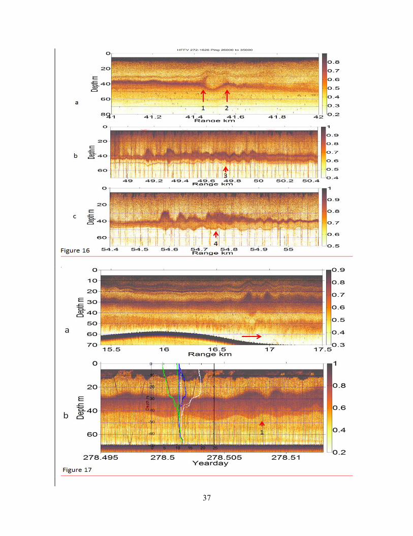
37

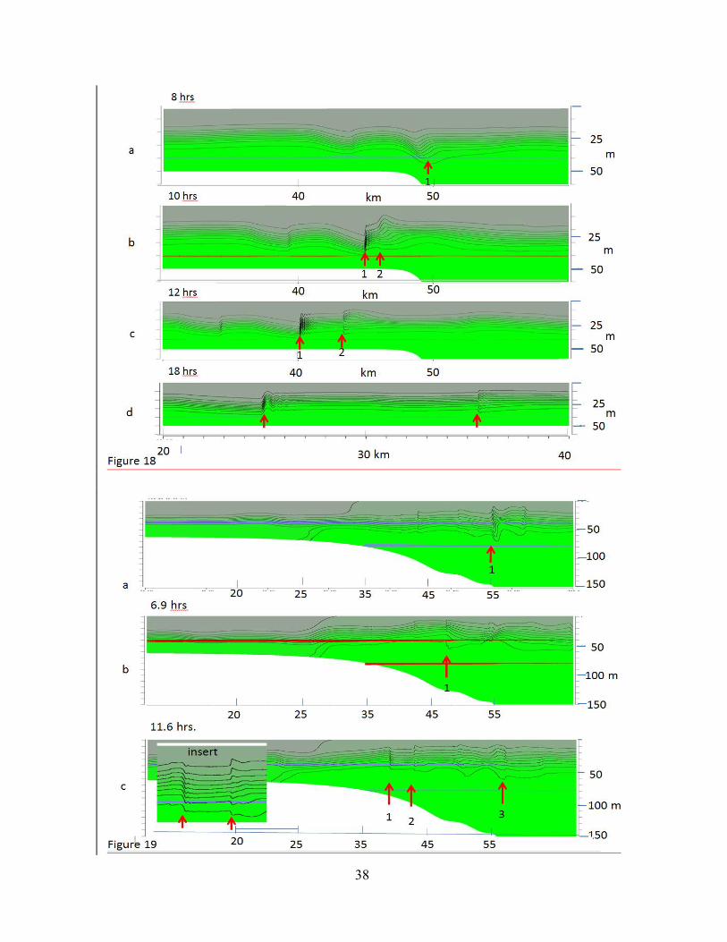
38

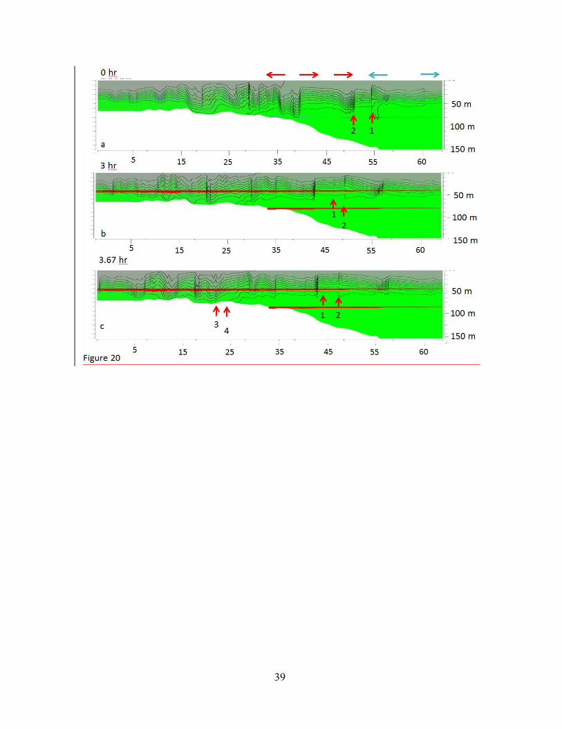
39