mmWave Radar for Automotive and Industrial Applications · mmWave Radar for Automotive and...
25
mmWave Radar for Automotive and Industrial Applications December 7, 2017 Karthik Ramasubramanian Distinguished Member of Technical Staff, Texas Instruments 1
Transcript of mmWave Radar for Automotive and Industrial Applications · mmWave Radar for Automotive and...

mmWave Radar for Automotive and Industrial Applications
December 7, 2017
Karthik Ramasubramanian
Distinguished Member of Technical Staff, Texas Instruments
1

Introduction • Radar technology has been in existence for several decades
– Military, Weather, Law enforcement, and so on
• In the past decade, use of radar has exponentially increased
– Automotive and Industrial applications
• Automotive applications
– Front-facing radar (LRR/MRR)
• Adaptive Cruise Control, Autonomous Emergency Braking
– Corner radar (SRR)
• Blind Spot Detection, Lane Change Assist, Front/Rear Cross
Traffic Alert
– Newer applications
• Automated parking, 360 degree surround protection
• Body/Chassis and In-cabin applications
• Industrial applications
– Fluid level sensing
– Solid volume identification
– Traffic monitoring and Infrastructure systems
– Robotics, and many others
2
LRR/MRR
SRR

77GHz mmWave Radar • mmWave: RF frequencies within 30 GHz to 300 GHz
– Wavelength is in the order of few millimeters
• 77GHz mmWave radar bands
– 76-77 GHz
• Allocated for vehicular radar in many countries
• Also available for infrastructure systems in certain regions
– 77-81 GHz
• Recently made available for short range radar
• Legacy 24 GHz UWB short range radar to be phased out by 2022
– 75-85 GHz: Available for level probing radar
• mmWave radar sensors can measure
– Radial distance (range) to the object
– Relative radial velocity to the object
– Angle of arrival using multiple TX, RX
• Some benefits of radar
– Robust to environmental conditions like dust/fog/smoke
– Operation in dazzling light, or no ambient light
– Operation behind plastic enclosure
3

FMCW Radar – Overview • Multiple types of radar modulation
waveforms used
– Pulsed radar, CW Doppler radar, UWB,
FSK, FMCW, PN-modulated radar
• FMCW: Frequency Modulated
Continuous Wave
– FMCW (sometimes called LFMCW or
Linear FMCW) is the most commonly
used scheme in automotive radar today
– Linear FMCW: TX signal has frequency
changing linearly with time (i.e., chirp)
4
fTx(t)
fRx(t)
fIF
(few MHz)
c
Rtd
2
Tchirp
t
B (in 100’s of
MHz or few
GHz)
FMCW – Freq vs. Time sawtooth pattern
• Key benefits of FMCW radar
– Ability to sweep wide RF bandwidth (GHz) while keeping IF bandwidth small (MHz)
• Better range resolution. RF sweep bandwidth of 2 GHz can achieve 7.5cm range resolution,
while IF bandwidth can still be <15MHz
– Lower peak power requirement, compared to pulsed radar

FMCW Radar – System Model (1/3)
• The transmitted FMCW waveform (chirp) is
• The instantaneous frequency of FMCW
waveform is
5
tT
Bf
dt
tdtf
c
c
TT
)(
2
1)(
t f T
(t)
B
Tc
1. TX signal
Tc
(s)duration Chirp
(Hz) chirp ed transmittofbandwidth Sweep
2cos)( 2
c
c
cT
T
B
tT
Btftx
T(t)
• High-level block diagram
Ramp
waveform
gen.
fc

FMCW Radar – System Model (2/3)
6
2. RX signal
• High-level block diagram
• Received signal is a scaled and delayed version of transmitted signal
• Round-trip delay of reflection td is
object) (from reflection ofdelay Time
nattenuatio lossPath
)()(2cos)()( 2
d
d
c
dcdTR
t
ttT
Bttfttxtx
R
R
light of Speed
object theof (Distance) Range
2
c
R
c
Rtd
fT(t)
fR(t)
fIF(t)
c
Rtd
2
Tc
t
Ramp
waveform
gen.

FMCW Radar – System Model (3/3)
7
3. Beat signal
(IF)
IF signal
• High-level block diagram
• Beat frequency or IF signal after receive mixer is as follows
R
R
fT(t)
fR(t)
fIF(t)
c
Rtd
2
Tc
t
)()(cos)()(cos2
)(
)(cos)(cos)()()(
ttttttty
ttttxtxty
TdTTdT
TdTTR
7
Filtered out in the
receiver
ttT
Bd
c
20
Can be calculated as
Beat frequency
corresponding to the target
Ramp
waveform
gen.

FMCW Radar – How it works (1/2)
8
• For static objects, the beat frequency is simply
proportional to the distance (round-trip delay)
• Beat frequency is the product of FMCW
frequency slope (B/Tc) and round-trip delay (td)
• For multiple objects, the beat signal is a sum of
tones, where each tone’s frequency is
proportional to the distance of the object
• The frequencies of these tones gives the
distances to the different objects
• Detection of objects and Distance (Range)
estimation is done typically by taking FFT of
received IF signal
Static objects
c
bT
B
c
Rf
2Beat freq = Round-trip delay * Slope

FMCW Radar – How it works (2/2)
9
• For moving objects, velocity (v) is determined using phase change across
multiple chirps
• Phase and frequency of the received beat signal for the nth chirp can be
calculated as
• Second dimensional FFT is performed across chirps to determine the phase
change and thus the velocity
Moving objects
ttT
BBnf
c
vTnf
c
vd
c
ccc
)(
22
220
Phase change from chirp-to-chirp
that depends only on the velocity
(not on range)
• The two-dimensional FFT process gives a
2D range-velocity image (FFT heatmap)
• Typically, detection of objects is done on
this image
• After detection, the range and relative
speed of the objects are easily calculated
New terms in beat frequency

Angle Estimation - Beamforming
• Consider received signal for multiple RX antennas (say, four) as shown in figure
• Additional distance (Δ) travelled at successive antennas depends on the angle of
arrival θ
• This additional distance results in a phase change (w) across consecutive antennas
• This phase change can be estimated (west) using an FFT (3rd dimension FFT)
• Once w is estimated, the angle of arrival (θ) can be derived easily
θ
d
Δ=dsin(θ)
Uniform linear array
A Aejw Aej2w
θ
Aej3w

Sample FMCW Radar processing flow (1/2)
11
• Typical processing flow used in FMCW (sawtooth) Radar signal processing
Pre-
processing (DC removal, Interf
mitigation)
1st dim FFT (Range FFT)
2nd dim FFT (Doppler FFT)
Log-Mag &
Detection (CFAR-CA /
CFAR-OS)
Angle
Estimation (3rd dim FFT)
Clustering,
Tracking (Higher layer
algorithms)
Raw point
cloud
Tracked
objects R
an
ge
(m
)
Relative Radial Velocity
Lo
ng
itu
din
al a
xis
(m
)
Lateral axis (m)
ADC
output
2D FFT heatmap

Sample FMCW Radar processing flow (2/2)
1D FFT processing is done inline. 2D-FFT, 3D-FFT & Detection for current frame.
CFAR or other proprietary algorithms often used for detection.
Active transmission time of chirps
(10~15 ms) Inter-frame time
(upto 25~30ms)
A frame consists of active transmission
time and idle inter-frame time.
Frame time (~40ms)
time
Rx1,2,3,4
First-
dim
en
sio
n F
FT
(Ra
nge
FF
T)
Second-dimension FFT
(Doppler FFT)
Radar data cube memory
• Typical (simple) FMCW chirp configuration consists of a sequence of chirps followed by idle time

Advantages of Fast FMCW modulation
13
• Slow FMCW (Triangular)
waveform used in many
legacy systems
– Chirp duration in ms,
instead of us
• Slow FMCW has
advantage of low DSP
MIPS requirement
– No two-dimensional FFT
processing
• However, it suffers from
ambiguity issues
– No elegant way of getting
range-doppler image
• Fast FMCW (Sawtooth)
waveform is preferred in
newer systems
• Fast FMCW has ability to
provide range-doppler
two dimensional image of
objects
Slow (Triangular) FMCW
Fast (sawtooth) FMCW

Radar system performance parameters
• Key parameters
– Max range
– Range resolution
– Range accuracy
– Max velocity
– Velocity resolution
– Velocity accuracy
– Field of view
– Angular resolution
– Angular accuracy
– Cycle time
Rmax
Rmax
R R
Vmax
v
R
V
R
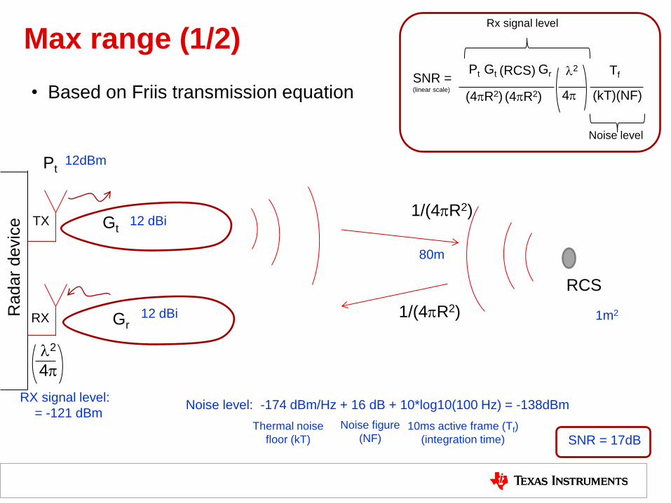
Max range (1/2)
• Based on Friis transmission equation
Pt
Gt 1/(4R2)
RCS
1/(4R2) Gr
2
4
12dBm
12 dBi
80m
1m2 12 dBi
RX signal level:
= -121 dBm
Radar
devic
e
Noise level: -174 dBm/Hz + 16 dB + 10*log10(100 Hz) = -138dBm
TX
RX
Thermal noise
floor (kT)
10ms active frame (Tf)
(integration time)
Noise figure
(NF)
Pt Gt
(4R2)
(RCS)
(4R2)
2
4
Gr
(kT)(NF)
Tf SNR = (linear scale)
Rx signal level
Noise level
SNR = 17dB

Max range (2/2)
• Max range depends on the below factors
Typical range
TX Output power 10 dBm – 13 dBm
TX Antenna gain 9 dBi – 23 dBi (USRR – LRR)
Depends on Azimuth and
Elevation field of view
RCS of target 0.1m2 – 50m2
(-10 dBsm to 17 dBsm)
Pedestrian vs. Truck
RX Antenna gain 9 dBi – 23 dBi Depends on Azimuth and
Elevation field of view
Noise figure 11 dB – 18 dB
Implementation dependent
Active frame time 2 ms – 20 ms
Detection SNR 10 dB – 18 dB
Pt Gt
(4)3
(RCS) Gr2
(kT)(NF)
Tf Rmax = 4 (SNR)
RX array beamforming gain can be additionally included.
Azim FOV (deg)
Elev FOV (deg)
Antenna gain (dB)
SRR 120 30 9.21
MRR 90 12 14.44
LRR 24 8 21.94
Target RCS
Pedestrian 0.1 ~ 1 sq.m
Motorbike 5 sq.m
Car 10 sq.m
Truck 50 sq.m
Thumb rule:
3 dB loss = 15% loss of range
12 dB loss = 50% loss of range

Range resolution and Range accuracy • Range resolution
– Ability to separate two closely spaced objects in
range
– Range resolution is a function of RF bandwidth
used
• Range accuracy
– Accuracy of range measurement of one object
– Depends on SNR
– Typically range accuracy is a small fraction of
range resolution
Sweep BW (MHz)
Range resolution (cm)
200 75
600 25
1000 15
2000 7.5
4000 3.75
B
cR
Tf
T
B
c
Rf
T
B
c
Rf
c
c
c
b
2 , therefore,
1But
2
2
c
bT
B
c
Rf
2
cTf
1
dB3
)( fH
f
c
bT
B
c
RRff
)(2
SNRB
cR
26.3

Max velocity • Max unambiguous velocity in Fast
FMCW modulation depends on chirp
repetition period
– Higher velocity needs faster ramps
• For a given max range and range
resolution, higher max velocity needs
higher IF bandwidth
• Advanced techniques are often used
to increase the max velocity
– Ambiguity resolution techniques can be
used to resolve aliased velocity into
true velocity
Total Chirp duration (us)
Max unamb velocity (+/-kmph)
50 70
38 92
25 140 cTv
4max
= wavelength
Tc = Total chirp duration
(incl. inter-chirp time)
Range
resolution
IF
bandwidth Max
unamb.
velocity
Max
range

Velocity resolution and Velocity accuracy
• Velocity resolution
– Ability to separate two objects in velocity
– Depends on the active duration of the frame
• Velocity accuracy
– Accuracy of velocity measurement of one object
– Depends on SNR
– Typically a fraction of velocity resolution
Active Frame duration (ms)
Velocity resolution (+/-kmph)
5 1.40
10 0.70
15 0.47
20 0.35 cNTv
2
= wavelength
N = number of chirps in the frame
Tc = Total chirp duration
(incl. inter-chirp time)
SNRNTc
v6.3

Benefits of 77GHz mmWave • Wide RF bandwidth (4 GHz) provides good range resolution and range accuracy
– 20X better than legacy 24GHz narrowband sensors (which use ~200MHz bandwidth)
• High RF frequency (small wavelength) provides good velocity resolution and accuracy
– 3X better than 24GHz sensors
• Smaller form-factor for the sensor
20
More focused beam with 77GHz
Improved performance
Better resolution performance with 77GHz

Angular resolution • Angular resolution
– Ability to separate objects in angle (for same range
and velocity)
– Radar sensors have poorer angular resolution
typically (compared to LIDAR for example)
– However, in many real life situations, objects get
resolved in range or velocity, due to good resolution
in those dimensions
– Angular resolution (in radians) for K-length array is
given by:
=λ
Kdcos(θ) Note the dependency of the resolution on θ.
Resolution is best at θ=0
=2
K Resolution is often quoted assuming d=λ/2 and θ=0
Array length Ang. Resolution (deg)
8 14.32
12 9.55
24 4.77
40 2.86
(in radians)

Use of Multiple TX – MIMO radar
Tx1 Tx2 Rx1 Rx4
2 /2 /2
8 virtual channels
• Multiple TX along with multiple RX (MIMO radar) to increase angular resolution – eg. 2 TX, 4 RX can give 8
virtual channels
Active transmission time of chirps
(Tx1 and Tx2 chirps interleaved) Inter-frame time
Frame time (~40ms)
time
Tx1 Tx2 Tx1 Tx2 Tx2
Active transmission time of chirps
(Tx1 and Tx2 BPM-coded, simultaneous transmission) Inter-frame time
Frame time (~40ms)
time
Tx1+Tx2 Tx1-Tx2 Tx1+Tx2
Multiple TX time-interleaved
Multiple TX BPM-multiplexed
• Multiple TX can also be used for TX beamsteering (simultaneous transmission with linear phase shifter
based steering of beam)

Cascaded multi-chip radar
23
8 channels (2 TX, 4 RX) 12 channels (3 TX, 4 RX)
24 channels (3 TX, 8 RX) 40 channels (5 TX, 8 RX) Master device Slave device (LO sync’ed to master)
TX RX TX RX Measurement results with 2 corner reflectors at ~4deg separation
Two corner reflectors 2-chip cascade radar
Single chip Single chip
2-chip cascade 2-chip cascade
2-chip cascade enables better separation of the corner reflectors

TI mmWave radar devices • TI offers a family of 77GHz radar devices for automotive and industrial applications
– Highly integrated devices based on RFCMOS
– High accuracy, Small form-factor, Sensing simplified
For more information, visit:
TI.com/mmWave

References • M. Skolnik, Introduction to Radar Systems, McGraw-Hill, 1981
• Donald E. Barrick, “FM/CW Radar Signals and Digital Processing”, NOAA Technical Report
ERL 283-WPL 26, July 1973
• A. G. Stove, ‘‘Linear FMCW radar techniques’’, IEE Proceedings F, Radar and Signal
Processing, vol. 139, pp. 343-350, October 1992
• M. Schneider, ‘‘Automotive Radar Status and Trends’’, in German Microwave Conference
(GeMiC), pp. 144-147, Ulm, Germany, April 2005
• TI whitepapers
– The fundamentals of millimeter wave – Available at http://www.ti.com/lit/spyy005
– Highly integrated 77GHz FMCW Radar front-end: Key features for emerging ADAS applications –
Available at http://www.ti.com/lit/spyy003
– TI’s smart sensors enable automated driving – Available at http://www.ti.com/lit/spyy009
– AWR1642: Radar-on-a-chip for short range radar applications – Available at http://www.ti.com/lit/spyy006
– Fluid-level sensing using 77 GHz millimeter wave – Available at http://www.ti.com/lit/spyy004
– Robust traffic and intersection monitoring using millimeter wave radar – Available at
http://www.ti.com/lit/spyy002
25