MIT18 03S10 Reading Lec29

18.03 Difference Equations and Z-TransformsJeremy Orloff

Difference equations are analogous to 18.03, but without calculus. On the last pageis a summary listing the main ideas and giving the familiar 18.03 analog. The twoline summary is:

1. In 18.03 the answer is eat, and for difference equations the answer is an.

2. The differential operator D has both algebraic and analytic analogs in differenceequations.

Sequences x[n] (also called signals or discrete functions)

Examples:

a)

. . .

•

•• • •

1234

−2 −1 0 1 2

. . .

x[n] = (1/2)n

⇒ . . . x[−2] = 4, x[−1] = 2,

x[0] = 1, x[1] = 1/2, . . .

b)

. . . • • •

•

•

1234

−2 −1 0 1 2

. . .

x[n] =

{0 if n < 0

2n if n ≥ 0

c) Unit sample:

δ[n] =

{1 if n = 0

0 otherwise . . .• •

•

• •

1

−2 −1 0 1 2. . .

d) Unit step:

u[n] =

{0 if n < 0

1 if n ≥ 0 . . .• •

• • •1

−2 −1 0 1 2. . .

Difference Equations

Example 1: y[n]− y[n− 1] = x[n]. (x = input, y = output)

Example 2: y[n] + 8y[n− 1] + 7y[n− 2] = x[n].

Example 3: y[n] + 8y[n− 1] + 7y[n− 2] = x[n]− x[n− 1].

Example 4: y[n]− ny[n− 1] = x[n]

Examples 1-3 are constant coefficient equations, i.e. linear time invariant (LTI).Example 4 is not constant coefficient. We will focus on constant coefficient equations.

(continued)

1

18.03 Difference Equations and Z-Transforms 2

In practice it’s easy to compute as many terms of the output as you want: thedifference equation is the algorithm.

Example: For the difference equation y[n] − 12y[n − 1] = u[n] find y[n] for n ≥ 0.

Assume rest IC y[−1] = 0.

(Here u[n] is the unit step function.)

answer: Rewrite the equation as y[n] = u[n] + 12y[n− 1].

Make a table: n -1 0 1 2 3 4 . . .

u[n] 0 1 1 1 1 1 . . .

y[n] 0 1 3/2 7/4 15/8 31/16 . . .

We have already seen difference equations with Euler’s formula. For example the IVPy′ = ky; y(0) = 1 becomes the difference equation

yn+1 = yn + khyn = (1 + kh)yn ⇔ yn+1 − (1 + kh)yn = 0.

Here instead of y[n] we wrote yn

Z-transform (analog of Laplace transform)

Let x[n] be a sequence. Its z-transform is X(z) =∑n

x[n]z−n.

(analogous to F (s) =

∫ ∞0

f(t)e−st dt; e−s ↔ z−1.)

When it’s useful we will denote the z-transform of x by Zx (similar to using Lx for Laplace).

Example 1: z-transform of δ[n] is 1.

Example 2: z-transform of u[n] is U(z) =∞∑n=0

z−n = 1 + z−1 + z−2 + . . . =1

1− z−1.

Example 3: If x[n] = 0 for n < 0 and x[n] = an for n ≥ 0 thenX(z) =∞∑n=0

anz−n =1

1− az−1.

Convolution

Start with two sequences x[n] and y[n] their convolution is defined as

(x ∗ y)[n] =∑k

x[k] y[n− k].

This arises in the following way. X(z) =∑k

x[k]z−k, Y (z) =∑m

y[m]z−m.

⇒ X(z)Y (z) =

(∑k

x[k]z−k

)(∑m

y[m]z−m

)=∑k

∑m

x[k]y[m]z−k−m =∑n

(∑k

x[k]y[n− k]

)z−n

i.e., X(z)Y (z) = Z(x ∗ y).

(continued)


Delay Operator (algebraic analog of D)

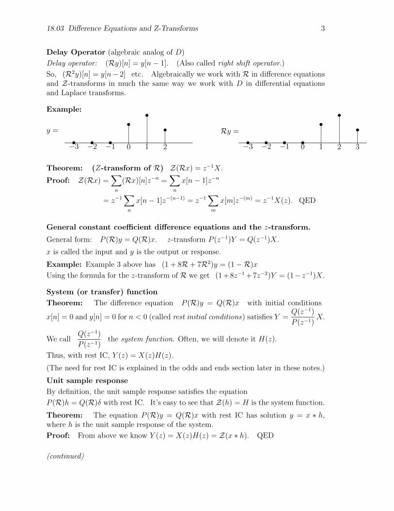
Delay operator: (Ry)[n] = y[n− 1]. (Also called right shift operator.)

So, (R2y)[n] = y[n− 2] etc. Algebraically we work with R in difference equationsand Z-transforms in much the same way we work with D in differential equationsand Laplace transforms.

Example:

y =

• • •

••

•

−3 −2 −1 0 1 2

Ry =

• • • •

••

•

−3 −2 −1 0 1 2 3

Theorem: (Z-transform of R) Z(Rx) = z−1X.

Proof: Z(Rx) =∑n

(Rx)[n]z−n =∑n

x[n− 1]z−n

= z−1∑n

x[n− 1]z−(n−1) = z−1∑m

x[m]z−(m) = z−1X(z). QED

General constant coefficient difference equations and the z-transform.

General form: P (R)y = Q(R)x. z-transform P (z−1)Y = Q(z−1)X.

x is called the input and y is the output or response.

Example: Example 3 above has (1 + 8R+ 7R2)y = (1−R)x

Using the formula for the z-transform of R we get (1 + 8z−1 + 7z−2)Y = (1− z−1)X.

System (or transfer) function

Theorem: The difference equation P (R)y = Q(R)x with initial conditions

x[n] = 0 and y[n] = 0 for n < 0 (called rest initial conditions) satisfies Y =Q(z−1)

P (z−1)X.

We callQ(z−1)

P (z−1)the system function. Often, we will denote it H(z).

Thus, with rest IC, Y (z) = X(z)H(z).

(The need for rest IC is explained in the odds and ends section later in these notes.)

Unit sample response

By definition, the unit sample response satisfies the equation

P (R)h = Q(R)δ with rest IC. It’s easy to see that Z(h) = H is the system function.

Theorem: The equation P (R)y = Q(R)x with rest IC has solution y = x ∗ h,where h is the unit sample response of the system.

Proof: From above we know Y (z) = X(z)H(z) = Z(x ∗ h). QED

(continued)


Example: Solve y[n]− ay[n− 1] = δ[n], with rest IC.

Z-transform: (1− az−1)Y = 1 ⇒ Y =1

1− az−1= 1 + az−1 + (az−1)2 + . . ..

⇒ y[n] =

{0 for n < 0

an for n ≥ 0

Poles, stability and homogeneous equations

The system P (R)y = Q(R)x has system function H(z) = Q(z−1)P (z−1)

.

So the poles of H(z) are exactly the roots of P (z−1).

(We need to assume P and Q have no common factors.)

As in differential equations these poles give us the solutions to the correspondinghomogeneous equation, i.e., P (R)y = 0.

Example: Solve the homogeneous equation P (R)y = y[n]+8y[n−1]+7y[n−2] = 0.

Trial solution: y[n] = an.

Substitution: an + 8an−1 + 7an−2 = 0 ⇒ an−2(a2 + 8a+ 7) = 0.

Characteristic equation: a2 + 8a+ 7 = 0.

Roots: a = −7, −1.

Two solutions: y1[n] = (−7)n, y2[n] = (−1)n.

General solution: y = c1y1 + c2y2. (This follows from the linearity of P (R).)

(Below we will discuss the existence and uniqueness theorem that guarantees thisgives all possible solutions.)

Note,1

P (z−1)=

1

1 + 8z−1 + 7z−2=

z2

z2 + 8z + 7. So the roots of the characteristic

equation are the same as the zeros of the denominator which are the poles of thesystem function.

Stability

As in 18.03, we say the system P (R)y = Q(R)x is stable if the homogeneous solutionyh[n]→ 0 as n→∞ no matter what the initial conditions.

That is, the initial conditions don’t affect the long-term behavior of the system.

Theorem: The system P (R)y = Q(R)x is stable if and only if all the poles ofthe system function have magnitude < 1. (We assume P and Q have no commonfactors.)

Proof: As in the example just above, the general homogenous solution is a linearcombination of sequences of the form yj[n] = anj , where aj is a pole of the systemfunction. This goes to 0 if and only if |aj| < 1.

(continued)


Graphically the system is stable if all the poles are inside the unit circle. (Comparethis with differential equations where the homogeneous solution is built from functionsof the form yj(t) = eat, so we need a in the left half-plane.)

Example:

Difference equations:

Re

Im

××××

Stable discrete system

Re

Im×

×

××

Unstable discrete system

Differential equations:

Re

Im

××

×

×Stable continuous system

Re

Im

××××

Unstable continuous system

Odds and ends

Causality: Causality means the future doesn’t affect the past. Our systemsP (R)y = Q(R)x are causal because y[n] depends only on y[k] and x[k] for k ≤ n.

Linearity: P (R) is linear, i.e. P (R)(c1y1 + c2y2) = c1P (R)y1 + c2P (R)y2.

Proof: Immediate from the definition of R and P (R).

Using linearity we see that the general solution to P (R)y = Q(R)x is given byy = yp + yh, where yp is any particular solution and yh is the general homogeneoussolution.

Example: Find the general solution to y[n]− 1

2y[n− 1] = u[n].

Homogeneous solution: Characteristic equation: a− 1

2= 0 ⇒ a =

1

2⇒ yh[n] = c

(1

2

)n

.

Particular solution: Use rest IC, so y[n] = 0 for n < 0.

We could find y[n] for n ≥ 0 directly, instead we’ll find it using the z-transform.

(1− 1

2z−1)Y =

1

1− z−1⇒ Y =

1

(1− 12z−1)(1− z−1)

=A

1− 12z−1

+B

1− z−1.

Using coverup we find A = −1, B = 2 ⇒ yp[n] =

{0 for n < 0

2− (1/2)n for n ≥ 0

Note, for n ≥ 0 we can write the answer in the form yp[n] = 1 +1

2+

1

4+ · · ·+

(1

2

)n

.

Finally, the general solution is y = yp + yh.

(continued)


Transient: If a system is stable then yh[n] → 0 for all initial conditions. In thiscase we call yh the transient.

Exponential Input Theorem: A solution to P (R)y = an is y[n] =an

P (a−1).

Proof: Ran = an−1 = a−1an ⇒ P (R)an = P (a−1)an.

(see below for the extended version of this theorem)

Discretizing DEs: In previous sections we have seen the algebraic analogy betweenthe differential operator D and the right shift operator R. That is, the algebra issimilar when dealing with either of these operators. But, for numerical methodswe need more than this. To discretize a differential equation we need to replaceD by something that is analytically analogous. You have already seen this whenwe learned Euler’s method. Here we will discretize DEs two different ways: usingforward differences and using backward differences. We will relate them to numericalmethods you have already learned. We will also discuss issues of stability.

Let yc(t) be a function of the continuous variable t.We can discretize yc by picking a stepsize h and a start time t0 and letting

y[n] = yc(t0 + nh).

Here are two ways to discretize the differential operator D (using the same stepsize h).

Forward difference: (∆f y)[n] =y[n+ 1]− y[n]

h, i.e. ∆f =

L − Ih

, where L is the

left shift operator.

Backward difference: (∆b y)[n] =y[n]− y[n− 1]

h, i.e. ∆b =

I −Rh

.

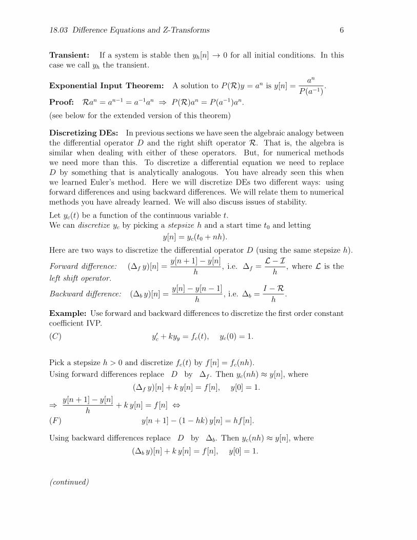
Example: Use forward and backward differences to discretize the first order constantcoefficient IVP.

(C) y′c + kyy = fc(t), yc(0) = 1.

Pick a stepsize h > 0 and discretize fc(t) by f [n] = fc(nh).

Using forward differences replace D by ∆f . Then yc(nh) ≈ y[n], where

(∆f y)[n] + k y[n] = f [n], y[0] = 1.

⇒ y[n+ 1]− y[n]

h+ k y[n] = f [n] ⇔

(F ) y[n+ 1]− (1− hk) y[n] = hf [n].

Using backward differences replace D by ∆b. Then yc(nh) ≈ y[n], where

(∆b y)[n] + k y[n] = f [n], y[0] = 1.

(continued)


⇒ y[n]− y[n− 1]

h+ k y[n] = f [n] ⇔ (1 + hk) y[n]− y[n− 1] = hf [n] ⇔

(B) y[n]− 1

1 + hky[n− 1] =

h

1 + hkf [n].

Example: (continued) Examine the stability of the original continuous system (C)and its discretized versions (F ), (B).

The continuous system (C) has system function1

s+ k. which has a pole at s = −k.

The homogeneous equation (the DE with fc(t) = 0) has solution yc = Ce−kt.

Looking at either the poles or the homogeneous solution we conclude the system isstable for k > 0.

The discrete system (F ) has system function1

1− (1− hk)z−1.

The system has a pole at z = 1− hk ⇒ it’s stable if |1− hk| < 1.

If k > 0 then we need 0 < h < 2/k for stability. Thus, even when (C) is stable, (F )is only stable for small h.

The discrete system (B) has system function1

1− z−1/(1 + hk).

The system has a pole at z = 1/(1 + hk) ⇒ it’s stable if 1/|1 + hk| < 1.

If k > 0 then (B) is stable for all h > 0. Thus, when (C) is stable so is (B) for any h.

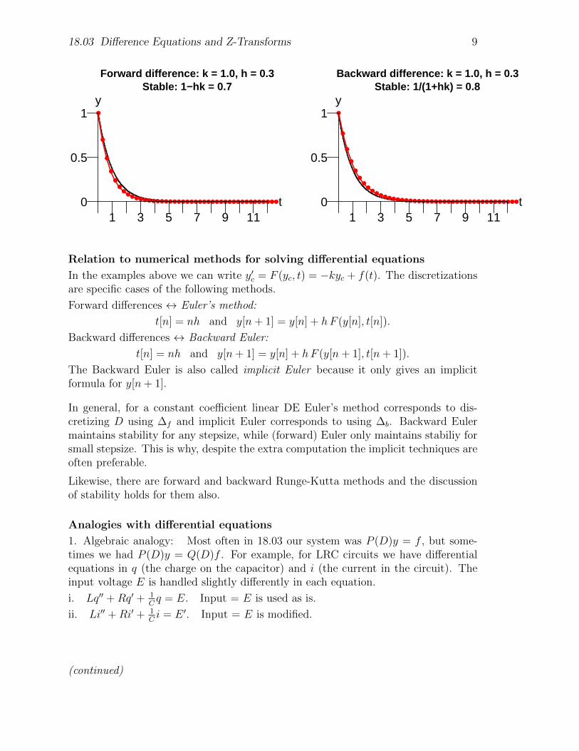
We can see the above results graphically by discretizing the homogeneous equationsusing various values of h. In all of the plots below, the black exponential curve is thecontinuous solution yc(t) = e−kt. Notice how, when discretizing a stable DE, forwarddifferences change quality as h decreases, while the backward differences do not.

(CH) y′c + ky = 0; yc(0) = 1 ⇒ yc(t) = e−kt.

(FH) y[n+ 1]− (1− hk) y[n] = 0; y[0] = 1 ⇒ y[n] = (1− hk)n

(BH) y[n]− 1

1 + hky[n− 1] = 0; y[0] = 1 ⇒ y[n] = (1 + hk)−n

Forward difference: k = 1.0, h = 2.1Unstable: 1−hk = −1.1

●

●

●

●

●

●

●

1 3 5 7 9 110

0.51

t

y

Backward difference: k = 1.0, h = 2.1Stable: 1/(1+hk) = 0.3

●

●

●

● ● ● ●

1 3 5 7 9 110

0.5

1

t

y

(continued)


Forward difference: k = 1.0, h = 2.0Unstable: 1−hk = −1.0

●

●

●

●

●

●

●

1 3 5 7 9 110

0.5

1

t

y


●

●

●

●● ● ●

1 3 5 7 9 110

0.5

1

t

y

Forward difference: k = 1.0, h = 1.5Stable, oscillatory: 1−hk = −0.5

●

●

●

●

●

●● ● ●

1 3 5 7 9 110

0.5

1

t

y


●

●

●

●● ● ● ● ●

1 3 5 7 9 110

0.5

1

t

y

Forward difference: k = 1.0, h = 0.8Stable: 1−hk = 0.2

●

●

●● ● ● ● ● ● ● ● ● ● ● ● ● ●

1 3 5 7 9 110

0.5

1

t

y


●

●

●

●

●● ● ● ● ● ● ● ● ● ● ● ●

1 3 5 7 9 110

0.5

1

t

y

(continued)


Forward difference: k = 1.0, h = 0.3Stable: 1−hk = 0.7

●

●

●

●

●

●●

●● ● ● ● ● ● ● ● ● ● ● ● ● ● ● ● ● ● ● ● ● ● ● ● ● ● ● ● ● ● ● ● ● ● ●

1 3 5 7 9 110

0.5

1

t

y


●

●

●

●

●

●

●●

●● ● ● ● ● ● ● ● ● ● ● ● ● ● ● ● ● ● ● ● ● ● ● ● ● ● ● ● ● ● ● ● ● ●

1 3 5 7 9 110

0.5

1

t

y

Relation to numerical methods for solving differential equations

In the examples above we can write y′c = F (yc, t) = −kyc + f(t). The discretizationsare specific cases of the following methods.

Forward differences ↔ Euler’s method:

t[n] = nh and y[n+ 1] = y[n] + hF (y[n], t[n]).

Backward differences ↔ Backward Euler:

t[n] = nh and y[n+ 1] = y[n] + hF (y[n+ 1], t[n+ 1]).

The Backward Euler is also called implicit Euler because it only gives an implicitformula for y[n+ 1].

In general, for a constant coefficient linear DE Euler’s method corresponds to dis-cretizing D using ∆f and implicit Euler corresponds to using ∆b. Backward Eulermaintains stability for any stepsize, while (forward) Euler only maintains stabiliy forsmall stepsize. This is why, despite the extra computation the implicit techniques areoften preferable.

Likewise, there are forward and backward Runge-Kutta methods and the discussionof stability holds for them also.

Analogies with differential equations

1. Algebraic analogy: Most often in 18.03 our system was P (D)y = f , but some-times we had P (D)y = Q(D)f . For example, for LRC circuits we have differentialequations in q (the charge on the capacitor) and i (the current in the circuit). Theinput voltage E is handled slightly differently in each equation.

i. Lq′′ +Rq′ + 1Cq = E. Input = E is used as is.

ii. Li′′ +Ri′ + 1Ci = E ′. Input = E is modified.

(continued)


In (i) we have P (D)q = E. In (ii) we have the more general P (D)i = Q(D)E, which

has system functionQ(s)

P (s). This is algebraically analogous to the difference equation

P (R)y = Q(R)x with system functionQ(z−1)

P (z−1).

2. Analytic analogy: This is covered in the section ’Discretizing DEs’ above. Therewe saw two ways to discretize D, D → ∆b and D → ∆f .

Theorem: (Existence and uniqueness) If P (R) has degree m then the IVP

P (R)y = 0; y[0] = b0, y[1] = b1, . . . , y[m− 1] = bn−1

has a unique solution.

Proof: This is clear. Simply solve for y[n] recursively as we did in the first order example.

We show a degree two example.

Example: Solve y[n] + a1y[n− 1] + a2y[n− 2] = 0, y[0] = b1, y[1] = b1.

General equation: y[n] = −a1y[n− 1]− a2y[n− 2].

y[0] = b0, y[1] = b1 ⇒ y[2] = −a1b0 − a2b2 ⇒ y[3] = −a1y[2]− a2y[1], etc.

We see that y[n] is uniquely determined.

Convolution formula as a result of linear time invariance

Consider the equation P (R)y[n] = Q(R)x[n] with rest IC. Let h be the unit sampleresponse. We will rederive the formula y = x ∗ h using linearity and time invariance.

Let y[n] = (x ∗ h)[n] =∑k

x[k]h[n− k].

The sequence h[n] is the solution to the equation P (R)y[n] = Q(R)δ[n].

Time invariance means that h[n− k] is a solution to P (R)y[n] = Q(R)δ[n− k].

We can write x[n] =∑k

x[k]δ[n− k], so by linearity we have

P (R)y[n] = P (R)∑k

x[k]h[n− k] =∑k

x[k]P (R)h[n− k] =∑k

x[k]Q(R)δ[n− k]

= Q(R)∑k

x[k]δ[n− k] = Q(R)x[n]

We have shown that y = x ∗ h is a solution.

(continued)


Growth and decay rates

If a is a complex number then if |a| < 1 the rate that an decays to 0 depends on|a|, the closer to 1 the slower an decays. Likewise if |a| > 1 the rate that an growsdepends on |a|.If a1, a2, . . . , am are complex numbers then the growth or decay rate of the linearcombination y[n] =

∑cja

nj is given by the biggest value of |aj|. If all |aj| < 1 then it

is a decay rate and the bigger the rate (the closer to 1) the slower y[n] decays.

Example: Both systems are stable. System A has a faster decay rate than systemB, i.e., the transient disappears faster for system A than for system B.

Re

Im

××

System A

Re

Im

×

×

System B

The need for rest IC: If y[n] is the solution to P (R)y = Q(R)δ then we needed

rest IC to write Y (z) =Q(z−1)

P (z−1). We’ll explain this using a simple example.

Consider P (R)y[n] = y[n]− y[n− 1] = δ[n].

Particular solution with rest IC: yp[n] =

{0 for n < 0

1 for n ≥ 0.

Homogeneous solution: yh[n] = c.

General solution: y[n] = yp[n] + yh[n] =

{c for n < 0

1 + c for n ≥ 0.

Since P (R)(yp + yh) = δ the z-transform gives P (z−1)(Yp + Yh) = 1. The reason we

can’t simply divide by P (z−1) is because P (z−1)Yh(z) = (1− z−1)∞∑

n=−∞

cz−n = 0.

Algebraically we say that P (z−1) and Yh(z) are zero divisors, that is, they are non-zero but when multiplied together they give 0. Just like dividing by 0, we have tobe careful doing division with zero divisors. By demanding rest IC we only considerz-transforms of sequences y with y[n] = 0 for n < 0. It is easy to see that this set(called a ring) does not have zero divisors.

(continued)


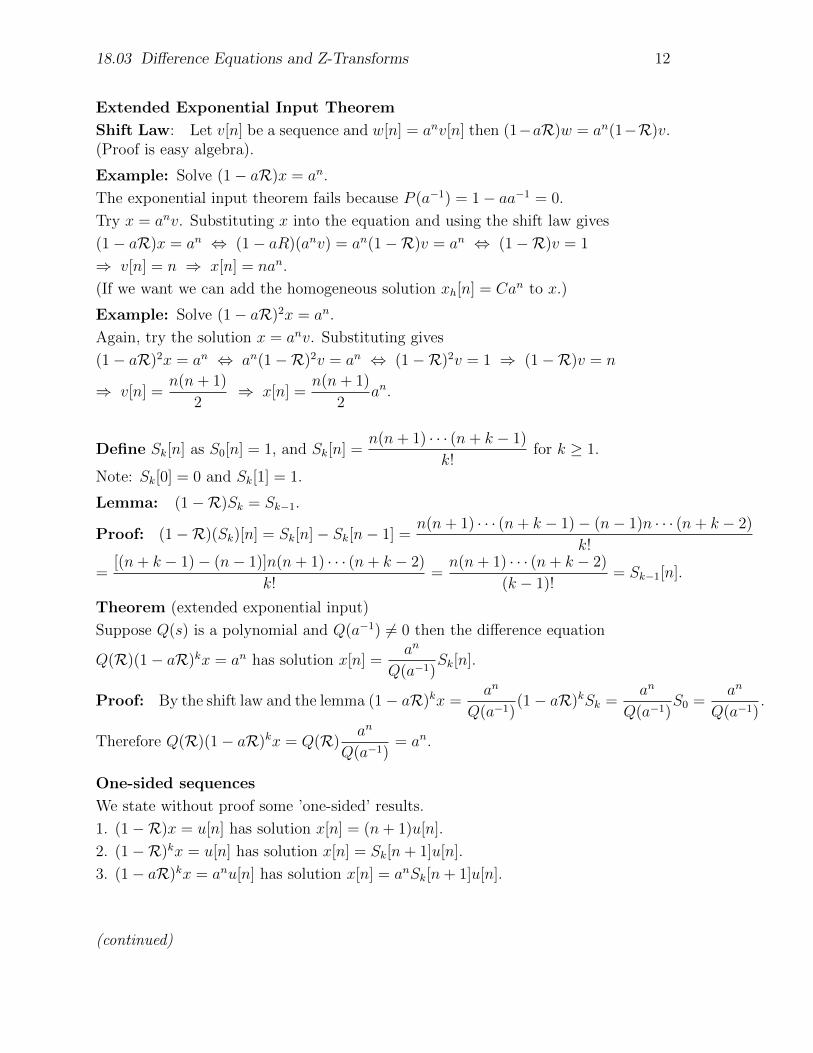
Extended Exponential Input Theorem

Shift Law: Let v[n] be a sequence and w[n] = anv[n] then (1−aR)w = an(1−R)v.(Proof is easy algebra).

Example: Solve (1− aR)x = an.

The exponential input theorem fails because P (a−1) = 1− aa−1 = 0.

Try x = anv. Substituting x into the equation and using the shift law gives

(1− aR)x = an ⇔ (1− aR)(anv) = an(1−R)v = an ⇔ (1−R)v = 1

⇒ v[n] = n ⇒ x[n] = nan.

(If we want we can add the homogeneous solution xh[n] = Can to x.)

Example: Solve (1− aR)2x = an.

Again, try the solution x = anv. Substituting gives

(1− aR)2x = an ⇔ an(1−R)2v = an ⇔ (1−R)2v = 1 ⇒ (1−R)v = n

⇒ v[n] =n(n+ 1)

2⇒ x[n] =

n(n+ 1)

2an.

Define Sk[n] as S0[n] = 1, and Sk[n] =n(n+ 1) · · · (n+ k − 1)

k!for k ≥ 1.

Note: Sk[0] = 0 and Sk[1] = 1.

Lemma: (1−R)Sk = Sk−1.

Proof: (1−R)(Sk)[n] = Sk[n]− Sk[n− 1] =n(n+ 1) · · · (n+ k − 1)− (n− 1)n · · · (n+ k − 2)

k!

=[(n+ k − 1)− (n− 1)]n(n+ 1) · · · (n+ k − 2)

k!=n(n+ 1) · · · (n+ k − 2)

(k − 1)!= Sk−1[n].

Theorem (extended exponential input)

Suppose Q(s) is a polynomial and Q(a−1) 6= 0 then the difference equation

Q(R)(1− aR)kx = an has solution x[n] =an

Q(a−1)Sk[n].

Proof: By the shift law and the lemma (1− aR)kx =an

Q(a−1)(1− aR)kSk =

an

Q(a−1)S0 =

an

Q(a−1).

Therefore Q(R)(1− aR)kx = Q(R)an

Q(a−1)= an.

One-sided sequences

We state without proof some ’one-sided’ results.

1. (1−R)x = u[n] has solution x[n] = (n+ 1)u[n].

2. (1−R)kx = u[n] has solution x[n] = Sk[n+ 1]u[n].

3. (1− aR)kx = anu[n] has solution x[n] = anSk[n+ 1]u[n].

(continued)


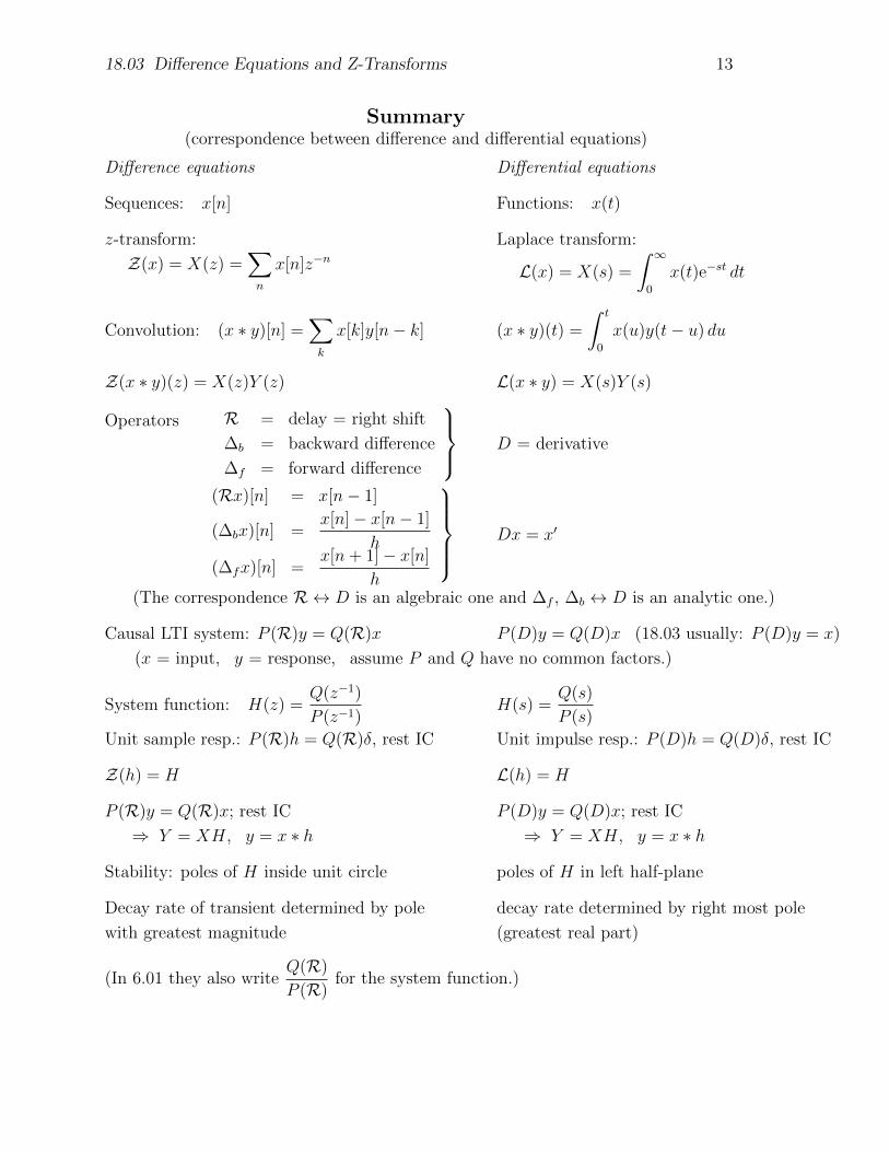
Summary(correspondence between difference and differential equations)

Difference equations Differential equations

Sequences: x[n] Functions: x(t)

z-transform:

Z(x) = X(z) =∑n

x[n]z−nLaplace transform:

L(x) = X(s) =

∫ ∞0

x(t)e−st dt

Convolution: (x ∗ y)[n] =∑k

x[k]y[n− k] (x ∗ y)(t) =

∫ t

0

x(u)y(t− u) du

Z(x ∗ y)(z) = X(z)Y (z) L(x ∗ y) = X(s)Y (s)

Operators R = delay = right shift

∆b = backward difference

∆f = forward difference

D = derivative

(Rx)[n] = x[n− 1]

(∆bx)[n] =x[n]− x[n− 1]

h

(∆fx)[n] =x[n+ 1]− x[n]

h

Dx = x′

(The correspondence R ↔ D is an algebraic one and ∆f , ∆b ↔ D is an analytic one.)

Causal LTI system: P (R)y = Q(R)x P (D)y = Q(D)x (18.03 usually: P (D)y = x)

(x = input, y = response, assume P and Q have no common factors.)

System function: H(z) =Q(z−1)

P (z−1)H(s) =

Q(s)

P (s)

Unit sample resp.: P (R)h = Q(R)δ, rest IC Unit impulse resp.: P (D)h = Q(D)δ, rest IC

Z(h) = H L(h) = H

P (R)y = Q(R)x; rest IC P (D)y = Q(D)x; rest IC

⇒ Y = XH, y = x ∗ h ⇒ Y = XH, y = x ∗ h

Stability: poles of H inside unit circle poles of H in left half-plane

Decay rate of transient determined by pole

with greatest magnitude

decay rate determined by right most pole

(greatest real part)

(In 6.01 they also writeQ(R)

P (R)for the system function.)

MIT OpenCourseWare http://ocw.mit.edu

18.03 Differential Equations �� Spring 2010

For information about citing these materials or our Terms of Use, visit: http://ocw.mit.edu/terms.

http://ocw.mit.edu

http://ocw.mit.edu/terms

MIT18 03S10 Reading Lec29

Documents

Transcript of MIT18 03S10 Reading Lec29